Matching E¢ ciency and Business Cycle Fluctuations · For useful comments, we thank Regis...

Matching Effi ciency and Business Cycle Fluctuations∗

Francesco Furlanetto† Nicolas Groshenny‡

May 2013

Abstract

We use a simple New Keynesian model with labor-market search to study the

macroeconomic implications of exogenous changes in the effectiveness of the process

through which unemployed workers are matched with vacant jobs. The importance

of these matching effi ciency shocks for unemployment fluctuations hinges critically

on the presence of pre-match hiring costs and nominal rigidities. Pre-match hiring

costs govern the magnitude of the unemployment response. Nominal rigidities affect

the sign of the vacancies’ response. For empirically plausible parametrizations of

these two key features, matching effi ciency shocks generate a positive correlation

between vacancies and unemployment and are thus an unlikely major source of

business cycle fluctuations. These disturbances may, however, help account for

specific episodes such as the recent period. A decline in matching effi ciency increases

inflation and raises the natural rate of unemployment above the actual rate, thus

calling unambiguously for a tightening of monetary policy.

Keywords: Search and Matching Frictions; Beveridge Curve; Reallocation Shocks.

JEL codes: E32, C51, C52

∗The views expressed in this paper do not necessarily reflect the views of Norges Bank. We areindebted to our discussants Tim Kam, James Hansen and Ian King for their extremely valuable feedback.For useful comments, we thank Regis Barnichon, Larry Christiano, Marco Del Negro, Punnoose Jacob,Nicolas Jacquet, Alejandro Justiniano, Francois Langot, Ellen McGrattan, Federico Ravenna, FabienTripier, Anders Vredin, Mirko Wiederholt, Jake Wong and seminar participants at the National Bank ofSerbia, University of Adelaide, Deutsche Bundesbank, Goethe University of Frankfurt, SWIM Auckland2012, AMW Monash 2012, WMD Sydney 2012 and the 2012 RBA Research Workshop on QuantitativeMacroeconomics.†Corresponding Author. Address: Norges Bank, Bankplassen 2, PB 1179 Sentrum, 0107 Oslo, Norway.

E-mail: [email protected]. Telephone number: +47 22316128.‡Address: University of Adelaide, School of Economics. E-mail: [email protected].

1

1 Introduction

In the aftermath of the Great Recession a number of policymakers have attributed un-

employment’s slow recovery to a decline in the effectiveness of the process that matches

unemployed workers and vacant jobs in the labor market (e.g. Kocherlakota 2010; Lacker

2012; and Plosser 2012). Recent studies provide some empirical evidence to support this

view.1 In this paper, we use a simple New Keynesian model with equilibrium search un-

employment to investigate the macroeconomic implications of changes in the effectiveness

of the labor market matching process.2 Like in the seminal paper by Andolfatto (1996),

we introduce a shock to the effi ciency of the matching function.

Unemployed workers, job vacancies, and matching effi ciency are related through the

aggregate matching function (cf. Blanchard and Diamond 1989; Petrongolo and Pissarides

2001). When matching effi ciency is low, for a given number of unemployed workers

and vacancies, fewer new jobs will be created. Therefore, matching effi ciency has an

interpretation that is similar to the Solow residual of the aggregate production function.3

However, while the literature has devoted a substantial effort to studying the production

function’s Solow residual and the properties of technology shocks, little is known about

1See for example Barlevy (2011), Barnichon and Figura (2011), Elsby, Hobijn, and Sahin (2010),Furlanetto and Groshenny (2013), Sahin, Song, Topa, and Violante (2012), Sala, Söderström, and Trigari(2012) and Veracierto (2011). Broadly, these studies suggest that matching effi ciency may have deterio-rated by roughly 20 percent. These studies reach different conclusions regarding the persistence of thisdecline. Several factors could explain a lower degree of matching effi ciency: skill mismatch (Sahin, Song,Topa and Violante, 2012, and Herz and van Rens, 2012), geographical mismatch, possibly exacerbatedby house-locking effects (Nenov, 2011), a reduction in search intensity by workers because of extendedunemployment benefits (Kuang and Valletta 2010; Fujita 2011), a reduction in firm recruiting intensity(Davis, Faberman, and Haltiwanger, 2010), a compositional change in unemployment due to a rise inpermanent layoffs and a larger share of long-term unemployment (Barnichon and Figura 2011).

2The use of search and matching frictions in business cycle models was pionereed by Merz (1995) andAndolfatto (1996) in the real business cycle (RBC) literature. More recently, these frictions have beenstudied in the New Keynesian model by Blanchard and Galí (2010), Christiano, Trabandt, and Walentin(2011), Christoffel, Kuester, and Linzert (2009), Gertler, Sala and Trigari (2008), Groshenny (2009 and2012), Krause and Lubik (2007), Krause, Lubik, and López Salido (2008), Ravenna and Walsh (2008 and2011), Sveen and Weinke (2008 and 2009), Trigari (2009), and Walsh (2005), among many others.

3Changes in matching effi ciency have an endogenous component, as is the case with the Solow residualof a production function (Basu, Fernald and Kimball, 2006). How to purify the residual of the matchingfunction is an interesting area for future research that is outside the scope of the current paper. Firstattempts in that direction are proposed by Borowczyk-Martins, Jolivet, and Postel-Vinay (2012), Chang(2012) and Sedlácek (2012).

2

the effects of shocks to the matching effi ciency. This paper aims to fill this gap.

Three main contributions emerge from our analysis. First, the propagation of shocks

to the matching effi ciency depends crucially on the form of hiring costs. When we consider

post-match hiring costs, in the form of training costs as in Gertler and Trigari (2009), we

show analytically that the shock does not affect unemployment and that the conditional

correlation between unemployment and vacancies is nil. When we consider pre-match

hiring costs in the form of the linear costs of posting a vacancy, as in Pissarides (2000),

the shock then affects unemployment and generates a positive correlation between unem-

ployment and vacancies. In the data, however, it is well known that this correlation is

strongly negative. Therefore, under both hiring cost specifications, shocks to the matching

effi ciency are unlikely to emerge as a main source of business cycle fluctuations. Never-

theless, these shocks can be seen as shifters of the Beveridge curve and may play a role

in specific episodes as long as pre-match hiring costs are not negligible.

Our second contribution is to show that when matching effi ciency shocks propagate,

i.e. under pre-match hiring costs, the presence of nominal rigidities is crucial for the

transmission mechanism. In fact, the response of vacancies can be positive or negative

depending on the degree of nominal rigidities present in the model. The sign of the va-

cancy response is important because it determines the conditional correlation between

unemployment and vacancies. When nominal rigidities are present, as in our baseline

model, a negative shock leads to an increase in vacancies and creates a positive corre-

lation. As we reduce the degree of nominal rigidities, the response of vacancies to a

negative disturbance becomes less and less positive and eventually turns negative when

prices are highly flexible. Hence, the conditional correlation between unemployment and

vacancies declines substantially and can even become negative when the shock has limited

persistence. Interestingly, this finding is reminiscent of Galí’s (1999) result on the role of

nominal rigidities for determining the sign of the employment response to a technology

shock.

Our third contribution concerns the role of monetary policy. Shocks to the matching

effi ciency, unlike the other shocks usually considered in the literature, propagate more in

models with flexible prices and wages than in models with nominal rigidities. Therefore,

3

the natural rate of unemployment reacts more than unemployment itself and a negative

matching effi ciency shock reduces the unemployment gap and increases inflation. If mon-

etary policy is based on standard intermediate targets, like inflation and unemployment

gap, a negative matching effi ciency shock calls for an increase in the policy rate.

Shocks to the matching effi ciency are already present in the seminal paper by Andol-

fatto (1996) that introduced search and matching frictions in the standard RBC model.

Since then, these shocks have also been considered in Beauchemin and Tasci (2012),

Krause, Lubik, and Lopez-Salido (2008), Lubik (2009), Cheremukhin and Restrepo-

Echevarria (2011), Justiniano and Michelacci (2011), and Mileva (2011), among others.

However, none of these papers relates the form of hiring costs and the degree of nomi-

nal rigidities to the propagation of matching effi ciency shocks. Importantly, our analysis

help explain why matching effi ciency shocks are responsible for a share of unemployment

fluctuations that are large in some estimated DSGE models (cf. Lubik 2009, and Krause,

Lubik, and López-Salido 2008) and limited in others (cf. Justiniano and Michelacci 2011;

Furlanetto and Groshenny 2013; and Sala, Södertröm, and Trigari 2012).

As argued by Andolfatto (1996), shocks to the matching effi ciency can be interpreted as

reallocation shocks as long as these capture some form of mismatch in skills, in geography,

or in other dimensions. Thus, our paper is also related to the literature initiated by

Lilien (1982) on the importance of reallocation shocks for business cycle fluctuations.

Abraham and Katz (1986) suggest that reallocation shocks play a limited role in explaining

aggregate fluctuations because these imply a positive correlation between unemployment

and vacancies (unlike aggregate demand shocks). However, their argument is not based

on a general equilibrium analysis. Here, we qualify the suggestion by Abraham and Katz

(1986) by showing that the sign of the conditional correlation between unemployment and

vacancies depends on the form of the hiring costs and the degree of nominal rigidities.

The paper proceeds as follows: Section 2 briefly describes the model, section 3 presents

our results, section 4 relates our results to the literature and section 5 concludes.

4

2 The Model

The model economy consists of a representative household, a continuum of intermedi-

ate good-producing firms, a continuum of monopolistically competitive retail firms, and

monetary and fiscal authorities which set monetary and fiscal policy, respectively. The

model is purposely simple. We ignore capital accumulation, real rigidities (such as habit

persistence and investment adjustment costs) and wage rigidities.4 Rather, in this paper

we concentrate only on the features that are critical for the transmission of matching ef-

ficiency shocks and leave aside the unnecessary complications. Our model’s version with

pre-match hiring costs is very similar to Kurozumi and Van Zandweghe (2010). The

version with post-match hiring costs is a simplified version of Gertler, Sala and Trigari

(2008).

The Representative Household The representative household is a large family,

made up of a continuum of individuals of measure one. Family members are either working

or searching for a job. The model abstracts from the labor force participation decision.

Following Merz (1995), we assume that family members pool their income before allowing

the head of the household to choose its optimal per capita consumption.

The representative family enters each period t = 0, 1, 2, ..., with Bt−1 bonds. At the

beginning of each period, bonds mature, providing Bt−1 units of money. The represen-

tative family uses some of this money to purchase Bt new bonds at nominal cost Bt/Rt,

where Rt denotes the gross nominal interest rate between period t and t+ 1.

Each period, Nt family members are employed. Each employee works a fixed amount

of hours and earns the nominal wage Wt. The remaining (1−Nt) family members are

unemployed and each receives nominal unemployment benefits b, financed through lump-

sum nominal taxes Tt. Unemployment benefits b are proportional to the steady-state

nominal wage: b = τW . The representative household owns retail firms and receives each

period the accumulated profits (Dt).

4We include all these features in a companion paper (Furlanetto and Groshenny 2013), where weestimate a medium-scale version of our model to study the evolution of unemployment during the GreatRecession and to quantify the importance of structural factors for unemployment dynamics.

5

The family’s period t budget constraint is given by

PtCt +Bt

Rt

≤ Bt−1 +WtNt + (1−Nt) b− Tt +Dt, (1)

where Ct represents a Dixit-Stiglitz aggregator of retail goods purchased for consumption

purposes and Pt is the corresponding price index.

The family’s lifetime utility is described by

Et

∞∑s=0

βs lnCt+s, (2)

where 0 < β < 1.

Intermediate Good-Producing Firms Each intermediate good-producing firm

i ∈ [0, 1] enters in period t with a stock of Nt−1 (i) employees. New matches become

productive in the period. Before production starts, ρNt−1 (i) old jobs are destroyed. The

job destruction rate ρ is constant. The workers who have lost their jobs start searching

immediately and can possibly still be hired in period t with a probability given by the job

finding rate. Alternatively, they will enter the unemployment pool before searching for a

job in the next period. This timing convention, proposed by Ravenna and Walsh (2008)

and used also by Sveen and Weinke (2009) and Christiano, Eichenbaum, and Trabandt

(2013), implies that our model features a kind of job-to-job transition mechanism that is

highly cyclical, given that it depends on the job-finding rate. Therefore, the flow from

employment to unemployment is not constant, as it increases during recessions, even if

we have a model with exogenous separation. Employment at firm i evolves according to

Nt (i) = (1− ρ)Nt−1 (i) + Mt (i) where the flow of new hires Mt (i) is given by Mt (i) =

QtVt (i) . The term Vt (i) denotes vacancies posted by firm i in period t and Qt is the

aggregate probability of filling a vacancy, defined as Qt = Mt

Vt.

The expressions Mt =∫ 1

0Mt (i) di and Vt =

∫ 1

0Vt (i) di denote aggregate matches and

vacancies respectively. Aggregate employment, Nt =∫ 1

0Nt (i) di, evolves according to

Nt = (1− ρ)Nt−1 +Mt. (3)

6

The matching process is described by an aggregate constant-returns-to-scale Cobb Douglas

matching function,

Mt = LtSσt V

1−σt , (4)

where St denotes the pool of job seekers in period t

St = 1− (1− ρ)Nt−1, (5)

and Lt is a time-varying scale parameter that captures the effi ciency of the matching

technology. It evolves exogenously following the autoregressive process,

lnLt = (1− ρL) lnL+ ρL lnLt−1 + εLt, (6)

where L denotes the steady-state value of the matching effi ciency, while ρL measures the

persistence of the shock, and εLt is i.i.d.N (0, σ2L).

The job-finding rate (Ft) is defined as Ft = Mt

Stand aggregate unemployment is Ut ≡

1 −Nt. Newly hired workers are immediately productive. Hence, the firm can adjust its

output instantaneously through variations in the workforce. However, firms face hiring

costs measured in terms of the finished good(Hkt (i)

), where k is an index to distinguish

the two types of hiring costs that we consider.

The first specification is a post-match hiring cost(Hpostt (i)

)in which total hiring costs

are given by

Hpostt (i) =

φN2

[Xt (i)]2Nt, (7)

where Xt (i) = QtVt(i)Nt(i)

represents the hiring rate.5 The parameter φN governs the magni-

tude of the post-match hiring cost. This kind of adjustment cost was first used by Gertler

and Trigari (2008) because it enables the derivation of the wage equation with staggered

contracts and helps the model fit the persistence and the volatility of unemployment and

5Post-match hiring costs are indexed to aggregate employment. All results are confirmed if they areindexed to employment at the firm level.

7

vacancies that we observe in the data (Pissarides 2009). This feature has become standard

in the empirical literature (cf. Christiano, Trabandt, and Walentin 2011; Gertler, Sala,

and Trigari 2008; Groshenny 2012; and Sala, Söderström, and Trigari 2008). The post-

match hiring cost can be interpreted as a training cost: it reflects the cost of integrating

new employees into the firm’s workforce.

The second specification that we consider is the hiring cost that is commonly used in

the literature on search and matching frictions (Pissarides, 2000). Following the classi-

fication in Pissarides (2009), it is a pre-match hiring cost (Hpret (i)) that represents the

cost of posting a vacancy. We use the following standard linear specification,

Hpret (i) = φNVt (i) . (8)

The parameter φN governs the magnitude of the pre-match hiring cost.

Each period, firm i uses Nt (i) homogeneous employees to produce Yt (i) units of in-

termediate good i according to the constant-returns-to-scale technology described by

Yt (i) = Nt (i) . (9)

Each intermediate good-producing firm i ∈ [0, 1] chooses employment and vacancies

to maximize profits and sells its output Yt (i) in a perfectly competitive market at a price

Zt(i) that represents the relative price of the intermediate good in terms of the final good.

The firm maximizes

Et

∞∑s=0

βsΛt+s+1

Λt+s

(Zt+s(i)Yt+s (i)− Wt+s (i)

Pt+sNt+s(i)−Hk

t+s(i)

), (10)

where Λt represents the marginal utility of consumption. Since the firm is owned by

the representative household, profits are discounted using the household’s discount factor(βsΛt+s+1

Λt+s

). Notice that all firms choose the same price and produce the same quantity.

8

Wage Setting The nominal wage Wt (i) is determined through bilateral Nash bar-

gaining,

Wt (i) = arg max[∆t (i)η Jt (i)1−η] , (11)

where 0 < η < 1 represents the worker’s bargaining power. The worker’s surplus, ex-

pressed in terms of final consumption goods, is given by

∆t (i) =Wt (i)

Pt− b

Pt+ βEt [(1− ρ) (1− Ft+1)]

(Λt+1

Λt

)∆t+1 (i) . (12)

The firm’s surplus in real terms is given by

Jt (i) = Zt (i)− Wt (i)

Pt− ∂Hk

t (i)

∂Nt (i)+ β (1− ρ)Et

[Λt+1

Λt

Jt+1 (i)

]. (13)

Retail Firms There is a continuum of retail goods-producing firms indexed by j ∈

[0, 1] that transform the intermediate good into a final good Y ft (j) that is sold in a

monopolistically competitive market at price Pt (j). Cost minimization implies that the

real marginal cost is equal to the real price of the intermediate good (Zt) that is common

across firms. Demand for good j is given by Y ft (j) = Ct(j) = (Pt(j)/Pt)

−θCt, where

θ represents the elasticity of substitution across final goods. Firms choose their price

subject to a Calvo (1983) scheme in which every period a fraction α is not allowed to

re-optimize, whereas the remaining fraction 1− α chooses optimally its price (P ∗t (j)) by

maximizing the following discounted sum:

Et

∞∑s=0

(αβ)sΛt+s

Λt

(P ∗t (j)

Pt+s− Zt+s

)Y ft+s (j) . (14)

All firms resetting prices in any given period choose the same price. The aggregate price

dynamics is then given by

Pt =[αP θ

t−1 + (1− α)P ∗t1−θ] 1

1−θ . (15)

9

Monetary and Fiscal Authorities The central bank adjusts the short-term nom-

inal gross interest rate Rt by following a Taylor-type rule,

ln

(Rt

R

)= ρr ln

(Rt−1

R

)+ (1− ρr)

[ρπ ln

(PtPt−4

)1/4

+ ρy ln

(YtYt−4

)1/4]. (16)

The degree of interest-rate smoothing ρr and the reaction coeffi cients to inflation and

output growth (ρπ and ρy) are all positive.

The government budget constraint takes the form

(1−Nt) b =

(Bt

Rt

−Bt−1

)+ Tt. (17)

Aggregate Resource Constraint The aggregate resource constraint reads as fol-

lows

Yt = Y ft +Hk

t , (18)

where Y ft =

∫ 1

0Y ft (j) dj. Notice that market clearing for each retail good implies that

Y ft (j) = Ct (j). Aggregating across firms, we obtain Y f

t = ΓtCt. Price dispersion across

firms

Γt ≡1∫

0

(Pt(j)/Pt)−θdj

drives a wedge between final output and consumption.

Parametrization Our parametrization is based on the US economy.6 A first set of

parameters is taken from the literature on monetary business cycle models. The discount

factor is set at β = 0.99, the elasticity of substitution across final goods at θ = 11 implies

a steady-state markup of 10 percent. The parameters in the monetary policy rule are

ρr = 0.8, ρπ = 1.5, ρy = 0.5. The average degree of price duration is four quarters,

corresponding to α = 0.75.

A second set of parameter values is taken from the literature on search and matching

6Our objective is not to calibrate parameters to match moments in the model and in the data. Suchan exercise would require the unrealistic assumption that the business cycle is driven only by shocks tothe matching effi ciency. Less ambitiously, our objective is to illustrate some simple economic mechanismsunder a plausible parametrization that is standard in the literature. Importantly, only two parameters(the degree of nominal rigidity and the autocorrelation in the shock process) can overturn the theoreticalmechanims described in the paper. We provide extensive sensitivity analysis to these parameters insection 4.

10

in the labor market. The degree of exogenous separation is set at ρ = 0.08, while the

steady-state value of the unemployment rate is U = 0.06. The elasticity in the matching

function is σ = 0.5, in the range of plausible values proposed by Petrongolo and Pissarides

(2001). In the absence of convincing empirical evidence on the value for the bargaining

power parameter η, we set it equal to 0.5 to satisfy the Hosios condition. The vacancy

filling rate Q is set equal to 0.70. We follow Blanchard and Galí (2010) by setting φN such

that total hiring costs in the steady state are equal to one percent of steady state output

in both models. The value of unemployment benefits τ is derived from the steady-state

conditions. These choices are common in the literature and avoid the indeterminacy issues

that are widespread in this kind of model, as shown by Kurozumi and Van Zandweghe

(2010) among others. Finally, the degree of persistence for the shock process is set at 0.6.

Table 1 summarizes our parametrization.

The log-linear first-order conditions that do not depend on the form of the hiring

cost function are listed in table 2. Lower scale variables stand for the capital variables

expressed in log-deviation from the steady state. In tables 3 and 4 we report the three

loglinearized first-order conditions that depend on the form of the hiring cost function

(the job creation condition, the wage equation, and the market-clearing condition). The

non linear equilibrium conditions are listed in appendix 3 together with the description

of the steady-state.

3 The Effects of Matching Effi ciency Shocks

In this section we present our three main results. In particular, we show how the effects

of matching effi ciency shocks on vacancies and unemployment depend crucially on the

nature of hiring costs and on the degree of nominal rigidities. Moreover, we discuss how

these results pose some implications for monetary policy.

3.1 Hiring Costs

In figure 1 we plot the impulse responses from a negative shock to the matching effi ciency

in the model with post-match hiring costs, as in Gertler and Trigari (2009) (dashed lines)

11

and in the model with pre-match hiring costs, as in Pissarides (2000) (solid lines).

The paper’s first result is that unemployment is invariant to the shock in the model

with post-match hiring costs, unlike what occurs in the model with pre-match hiring costs.

With post-match hiring costs, only vacancies and the probability of filling a vacancy react

to the shock. A negative shock to the matching effi ciency makes it more diffi cult to fill a

vacancy because the job market is less effi cient (qt decreases), but firms react by posting

more vacancies (vt increases) so as to keep the hiring rate (xt) constant. When expressed

in deviation from the steady state, the responses of the two variables in absolute values are

exactly of the same magnitude. This finding implies that employment does not react to

the shock and, in turn, that unemployment and output are also invariant to the shock. All

variables unrelated to the matching process remain unaffected by the matching effi ciency

shock. Put simply, the shock does not propagate.

With pre-match hiring costs it is still true that the probability of filling a vacancy

decreases and that firms react by posting more vacancies. However, in this case the two

effects do have not the same magnitude; a negative shock delivers a decrease in hiring

and an increase in unemployment. The shock behaves like a negative technology shock: a

less effi cient matching process in the labor market increases the firm’s marginal cost and

moves output and inflation in different directions. Overall, the shock has a contractionary

effect on the economy.

Why are hiring costs so important for propagating the shock? In a model with only

post-match hiring costs, it is costly for firms to integrate new employees whereas it is

costs nothing to post vacancies. A negative matching effi ciency shock directly reduces

the probability of filling a vacancy. In response to such shock, firms can avoid costly

fluctuations in hiring by posting more vacancies. Firms perfectly control the hiring rate

by varying vacancies. A shock to the matching effi ciency affects the magnitude of the

search frictions but this has no real consequences in the model because search is cost-free.

In the end, even if search frictions are present, these are inactive and the model behaves

like a model with employment adjustment costs.7 By contrast, in a model with pre-match

7This point can be seen analytically by combining the list of equilibrium conditions in tables 2 and3. In appendix 1 we show that unemployment dynamics do not depend on the matching function that isneeded only to study the behavior of vacancies.

12

hiring costs, search is costly and therefore fluctuations in the magnitude of the search

frictions have real consequences. In this case firms do not suffer costs from fluctuations

in hiring and find it optimal to decrease the hiring rate. In figure 2 we see that matching

effi ciency shocks generate a correlation between unemployment and vacancies which is

positive in the model with pre-match hiring costs and zero in a model with post-match

hiring costs.

A second perspective on the role of the hiring cost functions is given by comparing

the job creation conditions across the two models:

φNXt (1−Xt) +Wt

Pt= Zt + β (1− ρ)Et

Λt+1

Λt

φNXt+1, (19)

φVQt

+Wt

Pt= Zt + β (1− ρ)Et

Λt+1

Λt

φVQt+1

, (20)

where equation (19) refers to the model with post-match hiring costs while equation (20)

relates to the model with pre-match costs. On the left hand side we have the average cost

of hiring a worker; this consists of a wage component and a hiring cost component. The

hiring cost component is given by φNXt (1−Xt) in the model with post-match hiring

costs and by φVQtin the model with pre-match hiring costs. In the first case the firm is

able to minimize the hiring cost component by moving vacancies in such a way that the

hiring rate is constant. In the second case the hiring cost component is always positive

(which results in an output loss from the market clearing condition) and depends directly

on aggregate labor market conditions (Qt). In other words, the congestion externality

implied by the search frictions has real consequences. A negative shock raises the hiring

cost component of the marginal cost of hiring, so the firm reacts by reducing hiring.

Thus far we have investigated two polar cases: a model that only has post-match

hiring costs and a model with only pre-match hiring costs. Yashiv (2000) has proposed a

generalized hiring cost function that combines the two components in the following way,

13

Hgent (i) =

γ

2

[φV Vt (i) + (1− φV )Mt (i)

Nt (i)

]2

Nt, (21)

where γ relates to the size of total hiring costs8 and 0 ≤ φV ≤ 1 governs the importance of

the pre-match component. When φV is equal to 0 we revert to the model that only has the

post-match hiring costs described above. When φV is equal to 1 we obtain a model with

quadratic pre-match hiring costs.9 In figure 3 we consider this more general, and arguably

more realistic case, and plot the response of selected variables to a negative matching

effi ciency shock for different values of φV . We see that the choice of φV matters greatly for

determining the magnitude of the unemployment response. Importantly, unemployment

already reacts substantially for values of φV as low as 0.25. Silva and Toledo (2009)

and Yashiv (2000) estimate the relative shares of pre-match and post-match costs in total

hiring costs. Both studies find that post-match hiring costs account for at least 70 percent

of total hiring costs, suggesting that a realistic value for φV is around 0.3. The same result

is confirmed in an estimated New Keynesian model for Sweden by Christiano, Trabandt,

and Walentin (2011).

Overall, our analysis shows that empirical models of the business cycle that incorporate

unemployment should consider pre-match and post-match hiring costs in an integrated

framework. We do this in a companion paper (cf. Furlanetto and Groshenny 2013)

in which we estimate a medium-scale version of this model to study the evolution of

unemployment during the Great Recession and to quantify the importance of structural

factors for unemployment dynamics.

3.2 Nominal Rigidities

Having used the previous subsection to show how the nature of hiring costs affects the

propagation of matching shocks, we now restrict our attention to the simple model with

standard linear costs for posting vacancies and turn to the role of nominal rigidities. In

8γ is set such that total hiring costs in the steady state are equal to one percent of steady state output.9The derivations for the model with a generalized hiring cost function are provided in appendix 3.

14

figure 4 we plot impulse responses in the baseline model with sticky prices (solid lines)

and with flexible prices (dashed lines). The presence of sticky prices affects the sign of the

vacancy response. Under sticky prices firms do not increase prices as much as they would

prefer in response to a less effi cient matching process in the labor market. Therefore, the

decrease in output is limited. Given the reduced matching effi ciency, firms need to post

more vacancies to achieve their hiring target. When prices are flexible, firms can increase

prices optimally, so as to keep markups constant. The fall in aggregate demand is more

pronounced and firms need a larger contraction in hiring. To achieve this goal, firms cut

posted vacancies.

The importance of nominal rigidities for the sign of the vacancy response reminds us

of the debate regarding how employment responds to a technology shock in the standard

New Keynesian model. The analogy is justified by the fact that a matching effi ciency

shock can also be seen as a technology shock in the production of new hires. Galí (1999)

has linked the sign of the employment response to the presence of nominal rigidities and

inertia in monetary policy. When prices are rigid and monetary policy is not overly too

aggressive, a positive technology shock lowers employment. Alternatively, when prices are

flexible the labor market expands. Figure 4 shows that the same is true for the response

of vacancies to a matching effi ciency shock. The relationship between the sign of the

vacancy response and the degree of nominal rigidity can also be shown analytically in the

extreme (but still instructive) case where monetary policy is exogenous (instead of having

an interest rate rule) and prices are fixed (not sticky), closely following Galí (1999). The

derivation is provided in appendix 2.

Although a quantitative evaluation of the importance of matching effi ciency shocks

is not this paper’s objective, impulse responses in figure 4, particularly the sign of the

vacancy response, can provide some insights on the relevance of this shock. In fact,

unemployment and vacancies move in the same direction and they are almost perfectly

positively correlated (also see figure 2). It is well recognized that in the data unemploy-

ment and vacancies are strongly negatively correlated. This simple observation suggests

that shocks to the matching effi ciency are unlikely to emerge as a main source of busi-

ness cycle fluctuations in a model where prices are sticky. Nevertheless, these shocks can

15

be seen as shifters of the Beveridge curve with potentially important effects in specific

episodes. Recent analysis of the Beveridge curve dynamics through the lenses of DSGE

models and time-varying vector autoregressions (VARs) models are provided in Benati

and Lubik (2012) and Lubik (2011).

3.3 Policy Implications

Our previous results on the importance of the hiring costs specification and the degree

of nominal rigidities have implications for monetary policy that we model as a simple

Taylor-type rule. In the model with post-match hiring costs, inflation and output (to-

gether with unemployment) are invariant to shocks to the matching effi ciency. Therefore,

the monetary policy authority does not change the policy rate, even in presence of large

fluctuations in the matching effi ciency. Instead, when the pre-match hiring cost compo-

nent is not negligible, the monetary policy authority reacts to the shock by increasing

the policy rate to dampen inflationary pressures (despite the decrease in output). This

reasoning shows how important it is for central banks to understand the relative role of

different disturbances over the business cycle. When negative demand shocks (i.e. shocks

that move output and inflation in the same direction) are prevalent, the Taylor-type rule

prescribes an expansionary monetary policy. When negative matching effi ciency shocks

are present, monetary policy is contractionary in our model.

While studying the optimal policy response to matching effi ciency shocks is outside

the scope of the paper, it is interesting to discuss the implications for the unemployment

gap, which is a concept often present in the policy debate. Speeches by Kocherlakota

(2010), Bullard (2012), Lacker (2012), and Plosser (2011) allude to the possibility that

structural factors in the labor market have been responsible for a large decline in matching

effi ciency, which in turn has lead to an increase in the natural rate of unemployment.

According to these views, the unemployment gap, defined as the difference between actual

unemployment and the natural rate, may be low in the aftermath of the Great Recession

and expansionary monetary policies may not be appropriate. Our model can be used

to evaluate this hypothesis. Following the literature, we define the natural rate as the

16

rate of unemployment that emerges in a model with flexible prices and wages (cf. the

dashed lines in figure 4).10 In keeping with the framework used in the previous section,

we see that the natural rate of unemployment reacts more than the actual unemployment

rate in response to a negative disturbance.11 Therefore, a negative matching effi ciency

shock moves the inflation rate and the unemployment gap in opposite directions, while

a contractionary monetary policy simultaneously contributes to lower inflation and to

closing the unemployment gap.

In the policy discussion it is often said that monetary policy cannot do much to deal

with structural features of the labor market: "You can’t change the carpenter into a nurse

easily...monetary policy can’t retrain people. Monetary policy can’t fix these problems"

(Plosser 2011) or "I would go back to a single mandate. I think there is an overemphasis

on what the Fed can really do about unemployment" (Bullard 2012) or "There are many

possible sources of mismatch —geography, skills, demography...it is hard to see how the Fed

can do much to cure this problem" (Kocherlakota 2010). On the contrary, according to

our model, monetary policy has a role to play in response to a matching effi ciency shock

because its intermediate targets (inflation and the unemployment gap) are affected by

this kind of shock: the model prescribes a contractionary monetary policy response, at

least as long as the pre-match component in total hiring costs is not irrelevant.

Note, however, that our results should be interpreted very cautiously. Our prescription

is valid only conditional on the presence of matching effi ciency shocks while the available

empirical evidence seems to agree that these factors have played only a minor role in

recent years (cf. Barnichon and Figura 2012; Furlanetto and Groshenny 2013; and Sala,

Söderström, and Trigari 2012). If other shocks were responsible for the large increase

in unemployment during the Great Recession and for its slow decline in the recovery

period (for example negative financial shocks), an expansionary monetary policy may

be appropriate. Nevertheless, we believe that our paper elucidates some new theoretical

mechanisms that make the policy debate more transparent.

10This definition has been advocated also by Kocherlakota (2010).11Interestingly, the matching effi ciency shock is the only shock that can generate this pattern (cf.

Furlanetto and Groshenny 2013).

17

4 Our Results in Perspective

Our results presented in the previous section can be related to the debate on the impor-

tance of reallocation shocks initiated by Lilien (1982),12 according to whom these shocks

could explain up to 50 percent of unemployment fluctuations in the postwar period. The

empirical regularity underlying this result is a positive correlation between the disper-

sion of employment growth rates across sectors and the unemployment rate. However,

Abraham and Katz (1986) show that this positive correlation is consistent not only with

reallocation shocks but also with aggregate demand shocks under general conditions. Ac-

cording to Abraham and Katz (1986), data on unemployment and vacancies are more

useful to disentangling the importance of reallocation shocks. In fact, they argue that

reallocation shocks, unlike aggregate demand shocks, deliver a positive correlation be-

tween unemployment and vacancies as reallocation shocks can be seen as shifters of the

Beveridge curve along a positively sloped job creation line.13 Therefore, data on unem-

ployment and vacancies suggest the primacy of aggregate shocks, rather than reallocation

shocks. This argument has been used as an identifying assumption in VARs to reevalu-

ate the importance of reallocation shocks. Blanchard and Diamond (1989) conclude that

reallocation shocks play a minor role in unemployment fluctuations, at least at business

cycle frequencies (for a review of this literature, cf. Gallipoli and Pelloni, 2008).

Our paper contributes to the literature on the relationship between reallocation shocks

and the conditional correlation between unemployment and vacancies by highlighting the

different role of pre-match and post-match hiring costs and by using a fully specified

general equilibrium model, instead of a partial equilibrium model as used in the previous

literature. The distinction between pre-match and post-match hiring costs is crucial:

while both models imply an outward shift of the Beveridge curve, post-match hiring

costs generate a nil conditional correlation between unemployment and vacancies (given

12In this paper we follow the seminal contribution by Andolfatto (1996) and interpret the shock tothe matching effi ciency as a reallocation shock. This seems to be a natural choice in the context of aone-sector model. The same interpretation is given in Justiniano and Michelacci (2011), Furlanetto andGroshenny (2013), and Sala, Söderström, and Trigari (2012). An alternative and promising approach isthe use of multisector models that have, however, a less tractable structure (cf. Garin, Pries, and Sims2011).13The statement makes reference to a partial equilibrium model of the labor market with search and

matching frictions (cf. Jackman, Layard, and Pissarides 1989).

18

that unemployment is invariant to the shock) whereas pre-match hiring costs imply that

unemployment and vacancies move in the same direction (see figure 2). In that sense

our model qualifies the statement by Abraham and Katz (1986) by showing that the

sign of the conditional correlation between unemployment and vacancies depends on the

form of the hiring costs. Importantly, the use of a general equilibrium model is essential

for our conclusion. In fact, in a model with post-match hiring costs, the shift in the

Beveridge curve is accompanied by a general equilibrium effect on job creation that leaves

unemployment unaffected by the shock, whereas in the model with pre-match hiring costs

the two effects have different magnitudes and unemployment reacts to the shock.

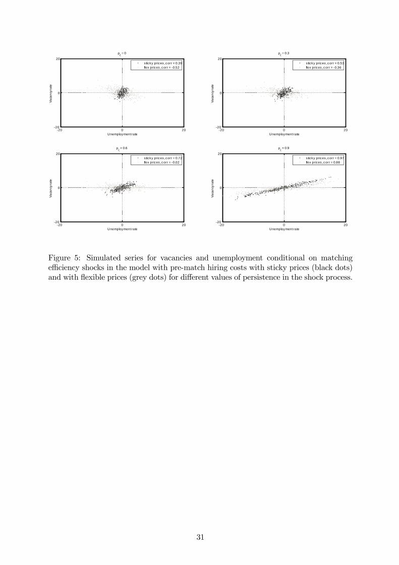
Furthermore, we provide a second contribution (specific to the model with pre-match

hiring cost) to the literature on reallocation shocks. As already anticipated, our base-

line model with sticky prices and pre-match hiring costs generates a positive conditional

correlation between unemployment and vacancies in response to a reallocation shock. In

figure 5 we appreciate that the sign of the correlation does not depend on the degree

of autocorrelation in the shock process. However, this result is not as general as the

previous literature has taken for granted. In fact, it relies on the presence of nominal

rigidities. From figure 5, we see that in a flexible price version of our model (α = 0),

the correlation between unemployment and vacancies depends on the degree of autocor-

relation in the shock process. When the shock process is very persistent, we confirm the

finding in Abraham and Katz (1986): the matching shock generates a positive conditional

correlation between unemployment and vacancies. But for lower degrees of persistence,

the correlation between unemployment and vacancies declines and becomes negative for

values of ρL lower than 0.6. When the shock is i.i.d, the conditional correlation between

unemployment and vacancies is -0.52, meaning that the sign of the conditional correlation

is in line with the one for the unconditional correlation. In figure 6 we see that the shock

generates a negative conditional correlation (blue areas) when persistence is limited and

when the degree of nominal rigidity is low.

Other papers have found that reallocation shocks do not necessarily imply a pos-

itive correlation between unemployment and vacancies. Hosios (1994) and Justiniano

and Michelacci (2011) have shown that in models with endogenous separation unemploy-

19

ment and vacancies can move in opposite directions in response to a reallocation shock.14

Therefore, data on unemployment and vacancies are inconclusive for identifying reallo-

cation shocks. Our paper shows that reallocation shocks can move unemployment and

vacancies in opposite directions even in a model with exogenous separation. However,

our distinctive contribution is on how the presence of nominal rigidities whose presence

generalizes the validity of the argument in Abraham and Katz (1986).

Finally, our paper contributes to the literature on estimated DSGE models with unem-

ployment for the United States in which different studies reach very different conclusions

on the importance of matching effi ciency shocks for unemployment fluctuations. Furlan-

etto and Groshenny (2013) and Sala, Söderström and Trigari (2012) find that they are

almost irrelevant. In Lubik (2009), matching effi ciency shocks explain 92 percent of un-

employment and 38 percent of vacancy fluctuations in a RBC model very similar to our

baseline model. Justiniano and Michelacci (2011) also estimate a RBC model for the

United States and for several other countries. However, in contrast to Lubik (2009),

they find that matching effi ciency shocks explain only 11 percent of unemployment fluc-

tuations in the United States.15 Our model can, at least in part,16 reconcile all these

different results: in Lubik (2009) hiring costs are only pre-match whereas in Justiniano

and Michelacci (2011) there is also a post-match component. According to our analysis,

the larger the weight of the post-match component is, the lower the importance of match-

ing effi ciency shocks should be, in keeping with the results in Lubik (2009) and Justiniano

and Michelacci (2011). Krause, Lubik, and López-Salido (2008) estimate a sticky price

version of the model in Lubik (2009) where prices are flexible. They find that match-

14Hosios (1994) uses a partial equilibrium model with temporary layoffs where the reallocation shock ismodeled as a shock to the relative price dispersion across firms. Justiniano and Michelacci (2011) proposea dynamic general equilibrium model with endogenous separation where the source of reallocation is ashock to the matching effi ciency, as in our model. Both papers include a shock to the separation rate asa second reallocation shock. Moreover, the two studies emphasize that reallocation shocks, unlike othershocks, move job finding rates and job separation rates in the same direction. Davis and Haltiwanger(1999) and Balakrishan and Michelacci (2011) use this comovement as an identifying assumption in aVAR. In our paper we concentrate on the role of hiring costs and nominal rigidities and we do not modelendogenous separation. In a model with endogenous separation the effect of a negative matching effi ciencyshock on unemployment is likely to be even smaller given that a lower job finding rate is accompaniedby a lower separation.15Similar numbers are found for Germany, Norway, and Sweden, but there is evidence of a somewhat

more important role for the matching effi ciency shock in France and in the United Kingdom.16The two models in Lubik (2009) and Justiniano and Michelacci (2011) are similar but not identical.

These differences can also influence the propagation of matching effi ciency shocks.

20

ing effi ciency shocks explain 37 percent of unemployment fluctuations. According to our

analysis, the model with sticky prices implies a positive conditional correlation between

unemployment and vacancies, whereas this is not always the case in a model with flexible

prices (it depends on the persistence of the shock that is not reported in Lubik 2009).

Therefore, our results can rationalize a more important role for matching effi ciency shocks

in RBC models. Finally, these shocks are almost irrelevant for output and unemployment

fluctuations in estimated models with a dominant post-match component in total hir-

ing costs and some degree of nominal rigidity, like Furlanetto and Groshenny (2013) and

Sala, Söderström, and Trigari (2012). These results are fully consistent with the theory

discussed in the previous section.

5 Conclusion

Our analysis of the transmission mechanism for shocks to the matching effi ciency empha-

sizes the importance of the form taken by the hiring cost function and the role of nominal

rigidities. In the extreme case when hiring costs are only post-match, the shock does not

propagate and matching effi ciency shocks are irrelevant for business cycle fluctuations.

When hiring costs include a pre-match component, the shock propagates and generates

a positive conditional correlation between unemployment and vacancies. This result is in

keeping with Abraham and Katz (1986), at least insofar as prices are sticky and the shock

is persistent. Importantly, a negative shock creates inflationary pressure and lowers the

unemployment gap, thus calling for a contractionary monetary policy response.

An interesting avenue for future research is to consider some of the determinants of

matching effi ciency in isolation. For example, the duration of the unemployment benefit17

and the search effort of workers and firms can be modeled explicitly in simple extensions

of the standard model. These exercises can be seen as a way to purify the matching

function’s Solow residual, as it has been done for the production function. In this sense,

the endogenous search effort can play the same role as endogenous capital utilization does

in the production function. We leave these extensions for future research.

17The role of extended unemployment benefits in the Great Recession is discussed in a recent paper byZhang (2013).

21

References

Abraham, K., Katz, L.F., 1986. Sectoral shifts or aggregate disturbances? Journal of

Political Economy 94, 507-522.

Andolfatto, D., 1996. Business cycles and labor market search. American Economic

Review 86, 112-132.

Balakrishan, R., Michelacci, C., 2001. Unemployment dynamics across OECD countries.

European Economic Review 45, 135-165.

Barlevy, G., 2011. Evaluating the role of labor market mismatch in rising unemployment.

Federal Reserve Bank of Chicago Economic Perspectives 3Q/2011.

Barnichon, R., Figura, A., 2011. Labor market heterogeneities, matching effi ciency and

the cyclical behavior of the job finding rate. Manuscript.

Barnichon, R., Figura, A., 2012. The determinants of the cycles and trends in US unem-

ployment. Manuscript.

Basu, S., Fernald J., Kimball, M., 2006. Are technology improvements contractionary?

American Economic Review 96, 5, 1418-1448.

Beauchemin, K., Tasci, M., 2012. Diagnosing labor market search models: a multiple

shock approach. Macroeconomic Dynamics, forthcoming.

Benati, L., Lubik, T., 2012. The time-varying Beveridge curve. Manuscript.

Blanchard, O.J., Diamond, P., 1989. The Beveridge curve. Brooking papers on Economic

Activity 1, 1-76.

Blanchard, O.J., Galí, J., 2010. Labor markets and monetary policy: a new Keynesian

model with Unemployment. American Economic Journal Macroeconomics 2, 1-30.

Borowczyk-Martins, D., Jolivet, G., Postel-Vinay, F., 2012. Accounting for endogenous

search behavior in matching function estimation. Review of Economic Dynamics, forth-

coming.

Calvo, G., 1983. Staggered prices in a utility maximizing framework. Journal of Monetary

Economics 12, 383-398.

22

Cheremukhin, A.A., Restrepo-Echevarria, P., 2011. The labor wedge as a matching fric-

tion. Manuscript.

Chang, B., 2012. A search theory of sectoral reallocation. Manuscript

Christoffel, K., Kuester, K., Linzert, T., 2009. The role of labor markets for euro area

monetary policy. European Economic Review, 53(8), 908-936.

Christiano, L.J., Eichenbaum, M., Trabandt, M., 2013. Unemployment and business

cycles. Manuscript.

Christiano, L.J., Trabandt, M., Walentin, K., 2011. Introducing financial frictions and

unemployment into a small open economy model. Journal of Economic Dynamics and

Control 35, 1999-2041.

Davis, S., Faberman, J., Haltiwanger, J., 2010. The establishment-level behavior of va-

cancies and hiring. NBER working paper 16265.

Davis, S.J., Haltiwanger, J., 1999. On the driving forces behind cyclical movements in

employment and job reallocation. American Economic Review 89, 1234-1258.

Elsby, M., Hobijn, B., Sahin, A., 2010. The labor market in the Great Recession. Brooking

Papers on Economic Activity, 1-48.

Fujita, S., 2011. Effects of extended unemployment insurance benefits: evidence from the

monthly CPS. Philadelphia Fed Working Paper 10/35.

Furlanetto, F., Groshenny, N., 2013. Mismatch shocks and unemployment during the

Great Recession. Manuscript.

Galí, J., 1999. Technology, employment and the business cycle: Do technology shocks

explain aggregate fluctuations? American Economic Review 89, 249-271.

Gallipoli, G., Pelloni, G., 2008. Aggregate shocks vs reallocation shocks: an appraisal of

the applied literature. RCEA working paper 27-08.

Garin, J., Pries, M., Sims, E., 2011. Reallocation and the changing nature of economic

fluctuations. Manuscript.

23

Gertler, M., Trigari, A., 2009. Unemployment fluctuations with staggered Nash wage

bargaining. Journal of Political Economy 117, 38-86.

Gertler, M., Sala, L., Trigari, A., 2008. An estimated monetary DSGE model with unem-

ployment and staggered nominal wage bargaining. Journal of Money, Credit and Banking

40, 1713-1764.

Groshenny, N., 2009. Evaluating a monetary business cycle model with unemployment

for the Euro area. Reserve Bank of New Zealand Discussion Paper Series 2009-08.

Groshenny, N. 2012. Monetary policy, inflation and unemployment. In defense of the

Federal Reserve. Macroeconomic Dynamics, forthcoming.

Herz, N., van Rens, T., 2012. Structural unemployment. Manuscript.

Hosios, A.J., 1994. Unemployment and vacancies with sectoral shifts. American Economic

Review 84, 124-144.

Jackman, R., Layard, R., Pissarides, C.A., 1989. On vacancies. Oxford Bulletin of Eco-

nomics and Statistics 51, 377-394.

Justiniano, A., Michelacci, C., 2011. The cyclical behavior of equilibrium unemployment

and vacancies in the US and Europe. NBER International Seminar on Macroeconomics

2011, The University of Chicago Press.

Kocherlakota, N., 2010. Back inside the FOMC. Speech available at

http://www.minneapolisfed.org/news_events/pres/speech_display.cfm?id=4525

Krause, M.U., Lubik, T.A., 2007. The (ir)relevance of real wage rigidity in the New

Keynesian model with search frictions. Journal of Monetary Economics 54, 706-727.

Krause, M.U., López-Salido, D., Lubik, T.A., 2008. Inflation dynamics with search fric-

tions: a structural econometric analysis. Journal of Monetary Economics 55, 892-916.

Kuang. K., Valletta, R., 2010. Extended unemployment and UI benefits. Federal Reserve

Bank of San Francisco Economic Letter.

Kurozumi, T., Van Zandweghe, W., 2010. Labor market search, the Taylor principle and

indeterminacy. Journal of Monetary Economics 57, 851-858.

24

Lacker, J.M., 2012. Maximum employment and monetary policy. Speech available at

http://www.richmondfed.org/press_room/speeches/president_jeff_lacker/2012/

lacker_speech_20120918.cfm

Lilien, D.M., 1982. Sectoral shifts and cyclical unemployment. Journal of Political Econ-

omy 90, 777-793.

Lubik, T.A., 2009. Estimating a search and matching model of the aggregate labor

market. Federal Reserve Bank of Richmond Economic Quarterly 95, 101-120.

Lubik, T.A., 2011. The shifting and twisting Beveridge curve: an aggregate perspective.

Manuscript

Merz, M., 1995. Search in the labor market and the real business cycle. Journal of

Monetary Economics 36, 269—300.

Mileva, M., 2011. Optimal monetary policy in response to shifts in the Beveridge curve.

Manuscript.

Nenov, P., 2011. Labor market and regional reallocation effects of housing busts. Manu-

script.

Petrongolo, B., Pissarides, C.A., 2001. Looking into the black box: an empirical investi-

gation of the matching function. Journal of Economic Literature 39, 390-431.

Pissarides, C.A., 2000. Equilibrium unemployment theory. MIT Press.

Pissarides, C.A., 2009. The unemployment volatility puzzle: is wage stickiness the an-

swer? Econometrica 77, 1339-1369.

Plosser, C., 2011. The Fed’s easy money skeptic. Interview available at http://online.wsj.com/

article/SB10001424052748704709304576124132413782592.html

Ravenna, F., Walsh, C., 2008. Vacancies, unemployment and the Phillips curve. European

Economic Review 52, 1494-1521.

Ravenna, F., Walsh, C., 2011. Welfare-based optimal monetary policy with unemploy-

ment and sticky prices: a linear quadratic framework. American Economic Journal

Macroeconomics 3, 130-162.

25

Sahin, A., Song, J.Y., Topa., G., Violante, G., 2011. Measuring mismatch in the US labor

market. Manuscript.

Sala, L., Söderström, U., Trigari, A., 2008. Monetary policy under uncertainty in an

estimated model with labor market frictions. Journal of Monetary Economics 55, 983-

1006.

Sala, L., Söderström, U., Trigari, A., 2012. Structural and cyclical forces in the labor

market during the Great Recession: cross-country evidence. NBER International Seminar

on Macroeconomics 2012, The University of Chicago Press.

Sedlácek, P., 2012. Match effi ciency and firms’hiring standards. Manuscript.

Silva, J.I., Toledo, M., 2009, Labor turnover costs and the cyclical behavior of vacancies

and unemployment. Macroeconomic Dynamics 13, 76-96.

Sveen, T., Weinke, L., 2008. New Keynesian Perspectives on Labor Market Dynamics.

Journal of Monetary Economics 55, 921-930.

Sveen, T., Weinke, L., 2009. Inflation and labor market dynamics revisited. Journal of

Monetary Economics 56, 1096-1100.

Trigari, A., 2009. Equilibrium unemployment, job flows and inflation dynamics. Journal

of Money, Credit and Banking 41, 1-33.

Van Rens, T., 2008. Comment on Gertler and Trigari. Manuscript.

Veracierto, M., 2011. Worker flows and matching effi ciency. Federal Reserve Bank of

Chicago Economic Perspectives 4Q/2011.

Walsh, C., 2005. Labor market search, sticky prices and interest rate rules. Review of

Economic Dynamics 8, 829-849.

Yashiv, E., 2000. The determinants of equilibrium unemployment. American Economic

Review 90, 1297-1322.

Zhang, J., 2013. Unemployment benefits and matching effi ciency in an estimated DSGE

model with labor market search frictions. Manuscript.

26

0 5 10 15 200.8

0.6

0.4

0.2

0M atching eff iciency shock

0 5 10 15 201.5

1

0.5

0

0.5Vacancy f illing rate

prem atchpost m atch

0 5 10 15 200

0.05

0.1

0.15

0.2

0.25Vacancies

0 5 10 15 200.01

0

0.01

0.02

0.03

0.04

0.05Unemployment

0 5 10 15 200.05

0.04

0.03

0.02

0.01

0

0.01O utput

0 5 10 15 200.05

0

0.05

0.1

0.15Inf lat ion

Figure 1: Impulse responses to a negative matching effi ciency shock in the model withpre-match hiring costs (solid lines) and in the model with post-match hiring costs (dashedlines). The standard deviation of the shock is set equal to 1 percent. Impulse responsesare expressed in percentage points.

27

20 0 2020

0

20

Unemployment rate (% dev from mean)

Vaca

ncy

rate

(% d

ev fr

om m

ean)

V and U condit ional on matching shocks

postmatchprematch

Figure 2: Simulated series for vacancies and unemployment conditional on matchingeffi ciency shocks in the model with post-match hiring costs (black dots) and in the modelwith pre-match hiring costs (grey dots).

28

0 5 10 15 200.7

0.6

0.5

0.4

0.3

0.2

0.1

0Matching ef f iciency shock

0 5 10 15 201.4

1.2

1

0.8

0.6

0.4

0.2

0

0.2Vacancy f illing rate

φV

= 0.01

φV

= 0.25

φV

= 0.50

φV

= 0.75

φV

= 0.99

0 5 10 15 200.05

0

0.05

0.1

0.15

0.2

0.25

0.3Vacancies

0 5 10 15 200

0.01

0.02

0.03

0.04

0.05

0.06

0.07

0.08Unemployment

Figure 3: Impulse responses to a negative matching effi ciency shock in the baseline modelwith a generalized hiring cost function. The standard deviation of the shock is set equalto 1 percent. Impulse responses are expressed in percentage points.

29

0 5 10 15 200.8

0.6

0.4

0.2

0Matching efficiency shock

0 5 10 15 201.5

1

0.5

0

0.5Vacancy filling rate

sticky pricesflex prices

0 5 10 15 200.2

0.1

0

0.1

0.2Vacancies

0 5 10 15 200

0.02

0.04

0.06

0.08

0.1

0.12Unemployment

0 5 10 15 200.12

0.1

0.08

0.06

0.04

0.02

0Output

0 5 10 15 200.05

0

0.05

0.1

0.15Inflation

Figure 4: Impulse responses to a negative matching effi ciency shock in the model withpre-match hiring costs with sticky prices (bold lines) and with flexible prices (dashedlines). The standard deviation of the shock is set equal to 1 percent. Impulse responsesare expressed in percentage points.

30

20 0 2020

0

20

Unemployment rate

Vaca

ncy r

ate

ρζ = 0

s ticky prices , corr = 0.39flex prices , corr = 0.52

20 0 2020

0

20

Unemployment rate

Vaca

ncy r

ate

ρζ = 0.3


20 0 2020

0

20

Unemployment rate

Vaca

ncy r

ate

ρζ = 0.6


20 0 2020

0

20

Unemployment rate

Vaca

ncy r

ate

ρζ = 0.9


Figure 5: Simulated series for vacancies and unemployment conditional on matchingeffi ciency shocks in the model with pre-match hiring costs with sticky prices (black dots)and with flexible prices (grey dots) for different values of persistence in the shock process.

31

0

0 . 2

0 . 4

0 . 6

0 . 8

1

0

0 . 5

1

1

0 .5

0

0 . 5

1

C a l v o p r o b a b i l i t yS h o c k p e r s i s t e n c e

Corr

(V,U

)

Figure 6: Conditional correlation between unemployment and vacancies (vertical axis) asa function of the degree of shock persistence (horizontal axis on the left) and of the degreeof nominal rigidity (horizontal axis on the right).

32

Table 1: Parametrization

Discount rate β 0.99

Elasticity of substitution between goods θ 11

Interest rate smoothing ρr 0.8

Response to inflation in the Taylor rule ρπ 1.5

Response to output growth in the Taylor rule ρy 0.5

Calvo coeffi cient for price rigidity α 0.75

Probability to fill a vacancy within a quarter Q 0.7

Separation rate ρ 0.08

Unemployment rate U 0.06

Elasticity of the matching function σ 0.5

Bargaining power η 0.5

Hiring costs to output ratio Hk

Y0.01

Matching shock persistence ρL 0.6

33

Table 2: Log-linearized first-order conditions

Euler equation ct = Etct+1 − (rt − Etπt+1) (T 1)

Production function yt = nt (T 2)

Law of motion for employment nt = (1− ρ)nt−1 + ρ(qt + vt) (T 3)

Definition of unemployment ut = −(NU

)nt (T 4)

Probability of filling a vacancy qt = lt − σ(vt +

((1−ρ)N

S

)nt−1

)(T 5)

Job finding rate ft = lt + (1− σ)(vt +

((1−ρ)N

S

)nt−1

)(T 6)

Definition of the hiring rate xt = qt + vt − nt (T 7)

New Keynesian Phillips curve πt = βEtπt+1 + κzt (T 8)

Monetary policy rule rt = ρrrt−1 + (1− ρr)(ρπ

14(pt − pt−4) + ρy

14

(yt − yt−4))

(T 9)

Matching effi ciency shock lt = ρLlt−1 + εL,t (T 10)

Table 3: Additional equations for the model with post-match hiring costs

xt = −(

WφNρ(1−2ρ)P

)(wt − pt) +

(Z

φNρ(1−2ρ)

)zt − β(1−ρ)

(1−2ρ)(rt − Etπt+1 − Etxt+1) (T 11)

wt − pt =(ηZPW

)zt +

(η2φNρ

2PW

)xt

−(ηβ(1−ρ)φNFρP

W

)(rt − Etπt+1 − Etxt+1 − Etft+1) (T 12)

yt =(

1− φNρ2

2

)ct + φNρ

2xt + φNρ2

2nt (T 13)

Table 4: Additional equations for the model with pre-match hiring costs

qt =(WQPφV

)(wt − pt)−

(ZQφV

)zt + β (1− ρ) (rt − Etπt+1 + Etqt+1) (T 14)

wt − pt =(ηZPW

)zt −

(ηβ(1−ρ)φV FP

WQ

)(rt − Etπt+1 + Etqt+1 − Etft+1) (T 15)

yt =(

1− φV VN

)ct + φV V

Nvt (T 16)

34

Table 5: Additional equations for the model with generalized hiring cost function(2(

1ρ− 1)(

φV VNΨ

vt + (1−φV )MNΨ

mt − nt)− 1

ρxt

)= −

(W

γΨ2P

)(wt − pt) +

(ZγΨ2

)zt

−β(1−ρ)ρ

(rt − Etπt+1 + Etxt+1 − 2

(φV VNΨ

Etvt+1 + (1−φV )MNΨ

Etmt+1 − Etnt+1

))(T 17)

wt − pt =(ηZPW

)zt +

(η2γPΨW

) (φV VNvt + (1−φV )M

Nmt −Ψnt

)−(ηβ(1−ρ)γFPΨ

Wρ

)[Ψ (rt − Etπt+1 + Etnt+1 − Etft+1)− 2φV V

NEtvt+1 −

((1− φV ) ρ− φV V

N

)Etmt+1

](T 18)

yt =(

1− γΨ2

2

)ct + γΨ

N(φV V vt + (1− φV )Mmt)− γΨ2

2nt (T 19)

where Ψ = φV V+(1−φV )MN

.

35

Appendix 1

The invariance of unemployment to matching effi ciency shocks in the model with post-

match hiring costs can be obtained analytically by using the list of equilibrium conditions

in tables 2 and 3. By substituting T7 into T3, we obtain

nt = nt−1 +ρ

1− ρxt, (22)

and by substituting T.5, T.6 and T.7 into T.12, we have

wt − pt =

(ηZP

W

)zt +

(η2φNρ

2P

W

)xt −

(ηβ (1− ρ)φNFρP

W

)(23)(

rt − Etπt+1 − 2Etxt+1 − Etnt+1 −(1− ρ)N

1− (1− ρ)Nnt

).

In the system of 9 equilibrium conditions (T1, T2, T4, T8, T9, T11, T13, 22 and 23)

with 9 endogenous variables, qt, ft and vt never appear. Therefore, that block of equations

is not affected by how the matching function is specified. More specifically, unemployment

dynamics are invariant to shocks to the matching effi ciency and to different values of the

elasticity in the matching function (σ). qt, ft and vt are determined residually by T5, T6

and T7.18

18This point was brought to our attention by Larry Christiano in a private conversation a few years ago.The same concept is expressed in a note written by Thjis Van Rens (2008) who also refers to a conversationwith Larry Christiano. At that time the point was relevant to understanding why unemployment volatilitywas higher in the model by Gertler and Trigari (2008) than in standard search and matching models andthere was no discussion on shocks to the matching effi ciency.

36

Appendix 2

The relationship between the sign of the vacancy response and the degree of nominal

rigidity can also be shown analytically in an extreme (but still instructive) case, following

Galí (1999) step-by-step. For the sake of the argument, we consider the case of exogenous

monetary policy (instead of an interest rate rule) and fixed prices (instead of sticky prices)

and we postulate the following equation for money demand in log-linear terms,

mt − pt = yt.

The assumptions of exogenous money and fixed prices imply that output is fixed in

the period. Given fixed output and exogenous technology, employment is also fixed (see

T.2). Then, from (T.3) there will be no job creation in response to the shock. Finally, the

response of vacancies to matching effi ciency shocks can be derived by using the matching

function. Being new hires fixed in the period and searchers a predetermined variable, the

following is true:

vt = − 1

(1− σ)lt.

According to our calibration (σ = 0.5), a one percent decrease in the matching effi -

ciency will be accompanied by a 2 percent increase in vacancies. Therefore, under the

extreme case of exogenous money and fixed prices, the vacancy response will be always

positive.19 This is also true in our model although the increase in vacancies is of course

lower, given that monetary policy is endogenous and prices are not fixed. Nevertheless,

the larger the degree of price rigidity is (and the more inertial monetary policy is), the

more positive the vacancy response will be (as the more negative the effect of a positive

technology shock on the labor input will be).20

19Notice that in this special case the distinction between pre-match and post-match hiring costs van-ishes: in both cases unemployment is invariant to shocks to the matching effi ciency.20Notice that the negative response of vacancies can be even larger in models with additional nominal

rigidities (sticky wages), real rigidities (habit persistence) and with capital accumulation (cf. Furlanettoand Groshenny 2013). Here, we prefer to use the simplest set-up to make our point more transparent.

37

Appendix 3

List of common equilibrium conditions in the symmetric equilibrium:

Λt = (Ct)−1

ΛtRt

= βEt

(Λt+1Πt+1

)Yt = Nt

Nt = (1− ρ)Nt−1 +QtVt

Ut = 1−Nt

St = 1− (1− ρ)Nt−1

Qt = Lt

(VtSt

)−σFt = Lt

(VtSt

)1−σ

P ∗t = θθ−1

Et∑∞s=0(αβ)sΛt+sP θt+sCt+sZt+s

Et∑∞s=0(αβ)sΛt+sP

θ−1t+s Ct+s

Pt =[αP θ

t−1 + (1− α)P ∗t1−θ] 1

1−θ .

Conditions specific to the model with post-match hiring costs

Yt = ΓtCt + φN2

[QtVtNt

]2

Nt

Wt

Pt= η

[Zt + φNX

2t + β (1− ρ)φNEt

Λt+1ΛtFt+1Xt+1

]+ (1− η) b

Pt

φNXt = Zt − Wt

Pt+ φNX

2t + β (1− ρ)φNEt

Λt+1ΛtXt+1.

Conditions specific to the model with pre-match hiring costs

Yt = ΓtCt + φV Vt

Wt

Pt= η

[Zt + β (1− ρ)Et

Λt+1ΛtFt+1

φVQt+1

]+ (1− η) b

Pt

φVQt

= Zt − Wt

Pt+ β (1− ρ)Et

Λt+1Λt

φVQt+1

.

Conditions specific to the model with generalized hiring cost function

Yt = ΓtCt + γ2

[φV Vt+(1−φV )Mt

Nt

]2

Nt

Wt

Pt= η

[Zt + γ


Nt

]2

+ β (1− ρ) γEtΛt+1ΛtFt+1

[φV Vt+1+(1−φV )Mt+1

Nt+1

]2Nt+1Mt+1

]+ (1− η) b

Pt

γ[φV Vt+(1−φV )Mt

Nt

]2NtMt

= Zt − Wt

Pt+ γ


Nt

]2

+ β (1− ρ) γEtΛt+1Λt

[φV Vt+1+(1−φV )Mt+1

Nt+1

]2Nt+1Mt+1

.

38

Steady state: common conditions

N = 1− U

Y = N

S = 1− (1− ρ)N

V = ρNQ

Z = θ−1θ

R = 1β

L = Q(VS

)σF = L

(VS

)1−σ.

Steady state: conditions specific to the model with post-match hiring costs

WP

= Z − φNρ (1− ρ) (1− β)

τ =WP−η(Z+φNρ

2+β(1−ρ)FρφN)(1−η)W

P

C = Y − φN2ρ2N.

Steady state: conditions specific to the model with pre-match hiring costs

WP

= Z − φVQ

(1− β (1− ρ))

τ =WP−η(Z+β(1−ρ)FφV Q

−1)(1−η)W

P

C = Y − φV V.

Steady state: conditions specific to the model with generalized hiring cost function

WP

= Z − γρ(φVQ

+ 1− φV)2

(1− ρ) (1− β)

τ =WP−η(Z+γρ2

(φVQ

+1−φV)2

+β(1−ρ)Fργ(φVQ

+1−φV)2)

(1−η)WP

C = Y − γ2ρ2(φVQ

+ 1− φV)2

N.

39

Matching E¢ ciency and Business Cycle Fluctuations · For useful comments, we thank Regis...

Documents

Transcript of Matching E¢ ciency and Business Cycle Fluctuations · For useful comments, we thank Regis...