Matching and Sorting in a Global Economy
69
Matching and Sorting in a Global Economy Gene M. Grossman Princeton University Elhanan Helpman Harvard University and CIFAR Philipp Kircher University of Edinburgh and London School of Economics April 14, 2013 Abstract We develop a neoclassical trade model with heterogeneous factors of production. We consider a world with two factors, managersand worker, each with a distribution of ability levels. Production combines a manager of some type with a group of workers. The output of a unit depends on the types of the two factors, with complementarity between them, while exhibiting diminishing returns to the number of workers. We examine the sorting of factors to sectors and the matching of factors within sectors, and we use the model to study the determinants of the trade pattern and the e/ects of trade on the wage and salary distributions and on measured pro- ductivity. Finally, we extend the model to include search frictions and consider the distribution of employment rates. Keywords: heterogeneous labor, matching, sorting, productivity, wage distribution, inter- national trade. JEL Classication: F11, F16 Part of this research was completed while Grossman was visiting STICERD at the London School of Economics and CREI at the University of Pampeu Fabra and while Helpman was visiting Yonsei University as SK Chaired Professor. They thank these institutions for their hospitality and support. The authors are grateful to Rohan Kekre, Ran Shorrer, and especially Kevin Lim for their research assistance. Finally, Grossman and Helpman thank the National Science Foundation and Kircher thanks the European Research Council for nancial support. 1
Transcript of Matching and Sorting in a Global Economy

Matching and Sorting in a Global Economy∗
Gene M. GrossmanPrinceton University
Elhanan HelpmanHarvard University and CIFAR
Philipp KircherUniversity of Edinburgh and London School of Economics
April 14, 2013
Abstract
We develop a neoclassical trade model with heterogeneous factors of production. We consider
a world with two factors, “managers”and “worker”, each with a distribution of ability levels.
Production combines a manager of some type with a group of workers. The output of a unit
depends on the types of the two factors, with complementarity between them, while exhibiting
diminishing returns to the number of workers. We examine the sorting of factors to sectors andthe matching of factors within sectors, and we use the model to study the determinants of the
trade pattern and the effects of trade on the wage and salary distributions and on measured pro-
ductivity. Finally, we extend the model to include search frictions and consider the distribution
of employment rates.
Keywords: heterogeneous labor, matching, sorting, productivity, wage distribution, inter-national trade.
JEL Classification: F11, F16
∗Part of this research was completed while Grossman was visiting STICERD at the London School of Economicsand CREI at the University of Pampeu Fabra and while Helpman was visiting Yonsei University as SK ChairedProfessor. They thank these institutions for their hospitality and support. The authors are grateful to Rohan Kekre,Ran Shorrer, and especially Kevin Lim for their research assistance. Finally, Grossman and Helpman thank theNational Science Foundation and Kircher thanks the European Research Council for financial support.
1
1 Introduction
In this paper, we study how international trade affects the sorting of heterogenous workers and
managers into industries and the matching of workers with managers in production units. It is
by now well known that firms in the same industry differ in size, in the compositions of their
workforces, in the technologies and capital goods they use, and in the wages they pay to their
workers. Industries differ in factor intensities and in the marginal contributions of worker and
managerial ability to firm productivity. Workers differ in physical attributes, in cognitive abilities,
and in their education, training, and experience. Although some studies of international trade have
examined the assignment of heterogeneous labor to different sectors and others have considered the
matching of workers to heterogeneous teammates or technologies, relatively little is known about
the general problem of how factors sort and match in the open economy when several of these
factors are differentiated, when fixed quantities of one impart decreasing returns to the others,
and when industries differ in their factor intensities and in the usefulness of factor “quality.”Our
paper addresses these more general, allocational issues and their implications for factor rewards.
Because workers and managers are heterogeneous, our analysis sheds light on the impact of trade on
the distribution of wages and managerial salaries, and thereby on the impact of trade on earnings
inequality.
By allowing for worker, manager, and industry heterogeneity, we can better understand a num-
ber of issues concerning the pattern and consequences of international trade. First, we can study
how countries’distributions of differentiated factors, in conjunction with their aggregate endow-
ments of these factors, determine their comparative advantage in the various sectors. Bombardini
et al. (2012) provide evidence, for example, that countries’skill dispersions have a quantitatively
similar impact on trade flows as do their aggregate endowments of human capital. Second, we can
investigate how trade influences factor returns across the entire income distribution, affecting more
than just the relative compensation paid to one factor versus another or to workers employed in one
industry versus another. These additional dimensions of inequality can be useful for understanding
recent findings of substantial variation in wages that is not easily explained by observable worker
characteristics. Helpman et al. (2012) show, for example, that within-industry wage variation
accounts for a majority of wage inequality in Brazil even after controlling for workers’occupations.
Finally, we can examine how globalization affects measured productivity in different sectors as a
result of the altered patterns of sorting and matching that are induced by trade. The effect of trade
liberalization on measured productivity has been the focus of much recent empirical research; see,
for example, Pavcnik (2002), Trefler (2004), and De Loecker (2011).
The literature on the sorting of workers to industries includes recent work by Costinot (2009),
Costinot and Vogel (2010), and Ohnsorge and Trefler (2007), as well as earlier work by Mussa
1
(1982) and Ruffi n (1988).1 All of these authors emphasize the comparative advantage that the
various types of labor have when employed in different industries. They study the determinants of
the trade pattern in countries that differ in the compositions of their labor forces and the impact
that trade has on income inequality across the skill or ability spectrum. But most assume a linear
relationship between labor input (of a given quality) and output or, what amounts to the same, an
absence of interactions between quantities of labor and quantities of other factors of production.
As emphasized by Eeckhout and Kircher (2012), models with one worker per firm or with a linear
relationship between labor quantity and output cannot speak to the determinants of a firm’s capital
intensity or its manager’s span of control.
Thematching of workers to technologies within an industry is the focus of work by Yeaple (2005)
and Sampson (2012). These authors also assume a production function with constant returns to
labor and thus omit interactions between labor and any other factors of production.2 Similarly,
Grossman and Maggi (2000) study the pairing of workers who perform different production tasks,
but in a context with exactly two workers per firm and therefore no scope for variation in factor
intensity or firm size. The work of Antràs et al. (2006) does allow for endogenous span of control in
a model with matching of workers and managers, but theirs is a one-sector model with international
production teams and they assume a particular technology that tightly links the quality and the
quantity of labor that a given manager can oversee.
Our analysis extends a familiar trade model with two sectors, two factors, and perfectly-
competitive product markets. While most of our analysis assumes frictionless factor markets,
we also consider an economy with search and matching frictions. We call one factor “labor”and
assume throughout that workers are differentiated along a single dimension that we term “ability.”
Workers with greater ability are assumed to be more productive in both industries, but the con-
tribution of ability to output may differ across uses. We refer to the second input as “managers.”
Similar to workers, managers generally differ in ability and more able managers contribute more
to output in both sectors, albeit to an extent that may vary by industry. With this formulation,
we can address how the economy matches a fixed but heterogenous supply of one input (managers)
with a fixed but heterogeneous supply of another (labor) in a setting where the relative number of
workers per manager is a matter for firms to decide.
In the next section, we lay out our basic model of an open economy with two countries, two
competitive industries, and two heterogeneous factors of production. Section 3 considers trade
between countries that have heterogeneous workers but homogeneous managers. Our analysis of
this simpler setting aids in understanding the more general case discussed in Sections 4 and 5,
where managers also are assumed to vary in ability. We show that, with homogeneous managers,
the sorting of workers is guided by a cross-industry comparison of the ratio of the elasticity of
1We use the term “sorting”to refer to the allocation of heterogeneous factors to different industries and the term“matching”to refer to the combination of differentiated factors within an industry.
2Both of these authors assume, however, that firms produce differentiated products in a world of monopolisticcompetition, so that inputs of additional labor by a firm do generate decreasing returns in terms of revenue. Thus,these models do share some features with the ones that we study below.
2

output with respect to labor quality to the elasticity of output with respect to labor quantity.
This can generate a simple sorting pattern in which all the best workers with ability above some
threshold level are employed in one sector and the remaining workers are employed in the other.
But it also can generate more complex patterns in which, for example, the most able and least able
workers sort to one sector while workers with intermediate levels of ability are allocated to the other.
Trade between countries with similar distributions of worker talent is determined by their aggregate
factor endowments as in the Heckscher-Ohlin model, whereas trade between countries with similar
relative endowments reveals a comparative advantage for a country with a superior distribution
of labor quality (as reflected in a proportional rightward shift of its talent distribution) in the
good produced by the industry in which worker ability contributes more elastically to productivity.
With homogeneous managers, relative price movements do not affect within-sector relative wages
and therefore have no effect on wage inequality within industries. Across industries, the impact of
trade on wages reflects a blend of Stolper-Samuelson and Ricardo-Viner forces, as in models with
imperfect factor mobility such as Mussa (1982) and Grossman (1983).
Section 4 addresses the sorting of heterogeneous workers and heterogeneous managers for the
special case in which the elasticity of output with respect to any factor’s ability is constant in both
industries. In obvious analogy with production functions based on quantities alone, we refer to
this as the Cobb-Douglas (productivity) case. In this setting, there is a unique sorting pattern
for each factor– which again reflects the ratio of a sector’s elasticity of output with respect to an
input’s ability and the elasticity of output with respect to the input’s quantity– but the matching
of workers and managers within an industry is not uniquely determined. Comparative advantage
again reflects relative aggregate endowments and the distributions of ability. An abundance of
managers per worker generates comparative advantage in the manager-intensive sector, whereas a
“better” distribution of some factor generates comparative advantage in the sector that exhibits
the greater elasticity of output with respect to that factor’s quality. In the Cobb-Douglas case, the
wages of workers and the salaries of managers in a given sector both rise with ability at constant
rates. These rates, which differ by factor and industry, reflect technological considerations alone.
It follows that trade has no impact on within-industry wage or salary inequality. Other dimensions
of factor rewards again are driven by a mix of Stolper-Samuelson and Ricardo-Viner forces.
In Section 5 we turn to the most interesting case, which has heterogeneity of both inputs
and productivity that is a strictly log supermodular function of the abilities of the production
unit’s manager and workers. Unlike the Cobb-Douglas case, the strong complementarities that are
captured by strict log supermodularity induce positive assortative matching in each sector. That
is, among the sets of workers and managers that sort to a given sector, the better workers are
matched with the better managers. We provide suffi cient conditions under which all of the workers
with ability above some threshold level and all the managers with ability above some (different)
threshold level sort to the same sector. We also provide conditions under which the high-ability
workers sort to the same sector as the low-ability managers. More complex sorting patterns are
possible as well. When countries share the same distributions of abilities and the sorting patterns
3

do involve a single threshold for each factor, then the country endowed with more managers per
worker must export the manager-intensive good.
When there are strong complementarities between the types of workers and managers, the effects
of trade or trade liberalization on the wage distribution are subtle and interesting. An increase in
the relative price of some good might worsen the matches for all workers and improve the matches
for all managers, or vice versa. Alternatively, a change in relative price might improve the matches
for workers in one industry while worsening those for workers in the other. We identify conditions
for these various shifts in the matching functions and discuss their implications for factor rewards.
In particular, we show that trade may cause within-industry income inequality to rise or fall and
the impact of trade on an input’s within-sector earnings inequality can differ from the changes that
occur across sectors.
In all of these settings, if the calculation of total factor productivity (TFP) fails to account for
factor heterogeneity, then trade will affect measured TFP in each industry and in the economy as
a whole. Consider, for example, a setting where the more able workers and managers sort into
the same sector in both countries, and the countries open to trade. The resulting price changes
induce workers and managers to move from the import-competing sector to the export sector in
each country. In the country where the import-competing sector employs the most able factors,
the marginal workers and managers that relocate are more able than those they join in their new
industry but less able than those that remain behind. Then average worker and manager quality
rise in each sector, and with them, measured TFP in each sector and in the economy as a whole.
Just the opposite happens in the other country, where average factor quality falls in both sectors.
Accordingly, trade can generate a convergence or divergence of measured productivity, depending on
the initial conditions and the patterns of comparative advantage, even if the underlying production
functions do not change. The effects on measured productivity in our model are reminiscent of
those in the seminal Roy (1951) model of labor sorting, except that here the changes in factor
composition occur due to trade.
In Section 6, we extend the analysis to include economies with labor-market frictions by assum-
ing that workers engage in directed search. In this setting, each potential worker seeks a job at a
firm of his choosing and manages to be hired by that firm with a probability that depends on the
number of applicants per vacancy. We show that, with these search frictions, wage and employment
rates both vary with ability; more able workers not only earn higher wages but also enjoy better
job prospects. Moreover, trade affects both wage and employment-rate inequality.
Section 7 contains some concluding remarks.
2 The Economic Environment
We examine a world economy comprising two countries, two industries, and two factors of pro-
duction. We call one of the factors “labor” and refer to individuals as “workers.” Each country
is endowed with a continuum of workers with various abilities. The exogenous supply of work-
4

ers of ability qL in country c is LcφcL(qL) for c = {A,B}, where Lc is the aggregate endowmentof labor and φcL (qL) is the density of workers with ability qL. For ease of exposition, we assume
throughout that φcL (qL) is continuous and strictly positive on its finite support ScL = [qcLmin, qcLmax],
where 0 < qcLmin < qcLmax < +∞. We refer to the second factor as “managers.”Country c hasa continuum of managers of measure Hc. We begin in Section 3 by assuming that all managers
are alike. Subsequently, we introduce manager heterogeneity and then denote the density of man-
agers with ability qH by φcH(qH), with φcH(qH) continuous and strictly positive on its finite support
ScH = [qcHmin, qcHmax].
3
Firms in the two countries have access to the same constant-returns-to-scale technologies. Out-
put per manager in an industry reflects the number of workers that is combined with a manager
there and the abilities of the inputs that are used in the production process. Specifically, when
a firm combines a manager with a group of workers, it must allocate a fraction of the manager’s
“time” to each of the workers. The greater is the fraction of managerial time that is devoted to
a worker, the greater is his productivity, but with diminishing returns. This formulation, which
is familiar from previous models of a manager’s “span of control” such as Sattinger (1975), Lu-
cas (1978) and Garicano (2000), implies that firms will combine a given manager with a group
of workers of uniform type and will divide the manager’s time evenly among them.4 To conserve
on notation, we invoke this implication of the firm’s optimal combination of inputs and write the
output in sector i of a manager of ability qH who is teamed with ` workers of (a common) type qLas5
xi = ψi (qH , qL) `γi , 0 < γi < 1, (1)
where γi < 1 is a parameter that reflects the diminishing returns from dividing the manager’s time
more finely and ψi (qH , qL) is a strictly increasing, twice continuously differentiable, log supermod-
ular function that captures the complementarities between the types of the two factors. We assume
that factor type contributes to productivity in qualitatively the same way in both sectors and,
without further loss of generality, order the types so that ∂ψi/∂qF > 0 for i = 1, 2 and F = H,L.
With this labeling convention, we refer to qF as the “ability”of factor F . Note that the industries
generally differ in the strength of the complementarities between factors, in the contributions of
factor abilities to productivity, and in their factor intensities.
The rest of the model is familiar from neoclassical trade theory. Consumers worldwide share
3We focus on an environment where factor endowments are invariant to trade. This makes our results comparableto most previous studies. Future work might consider adjustments in factor endowments - e.g., taking the terminologyof workers and managers literally one might study long-run skill acquisition that turns workers into managers.
4The key assumption here is that there is no teamwork or synergy between workers in a firm; they interact onlyin the sense that they compete for the time of the manager. See Eeckhout and Kircher (2012) for more discussion. Insuch circumstances, the primitive for technology gives output as a function of the type of the manager and types of allworkers with which it is combined. But there is no need for us to develop notation for this more general formulationsince we know that, in our setting, a firm will not gain (and typically will lose) by choosing to combine a given typeof manager with a variety of types of workers.
5We adopt a Cobb-Douglas-in-quantities specification in order to simplify the analysis. Some of our results wouldremain the same with an arbitrary constant-returns-to-scale production technology provided that there are no factorintensity reversals.
5

identical and homothetic preferences. Firms hire workers and managers on frictionless national
factor markets and engage in perfect competition on integrated world product markets. Countries
trade freely, with balanced trade. Note that we neglect for now the search frictions that are a
realistic and interesting feature of many markets with heterogeneous factors. We shall extend the
analysis to incorporate such frictions in Section 6 below.
3 Homogeneous Managers
We are ultimately interested in the sorting and matching of two heterogeneous factors of production.
However, before we get to that, we consider a simpler case in which there is no variation in the types
of one of the factors. By examining a setting with homogeneous managers we can gain insight into
the sorting of the heterogeneous workers into different sectors without needing to concern ourselves
with the matching of managers and workers. We will introduce manager heterogeneity in Section
4 below.
Suppose that all managers are interchangeable and assume, without further loss of generality,
that their common ability level is qH = 1. Let ψi(qL) ≡ ψi (qL, 1) be the productivity in sector i
of workers of ability qL when combined with any manager who might be employed there. Output
per manager in sector i can now be written as xi = ψi(qL)`γi , considering the diminishing returns
to the manager’s time.
A key variable in the analysis will be the ratio of two elasticities that describe a sector’s pro-
duction technology. One elasticity is εψi(qL) ≡ qLψ′i(qL)/ψ (qL), which reflects the responsiveness
of output to worker ability in sector i, holding constant the number of workers per manager. The
other elasticity is γi, which is the responsiveness of output to labor quantity, holding constant the
ability of the workers. Let
sL(qL) ≡εψ1
(qL)
γ1−εψ2
(qL)
γ2
be the difference across sectors in these ratios. We assume for now that sL (qL) has a uniform sign
for all qL in the domain of the ability distribution and label the industries so that sL (qL) > 0.
More formally, we adopt for now the following assumption:
Assumption 1 SH = {1} and sL (qL) > 0 for all qL ∈ SAL ∪ SBL .
A firm in sector i chooses the ability and number of its workers (per manager) to maximize
πi (qL, `) = piψi (qL) `γi − w (qL) ` − r, where pi is the price of good i, w (qL) is the wage of a
worker with ability qL, and r is the salary of the representative manager.6 We solve the firm’s
profit maximization problem in two stages. First, we calculate the optimal demand (per manager)
for workers of ability qL when the wage of such workers is w (qL), which yields
`i (qL) =
[γipiψi (qL)
w (qL)
] 11−γi
. (2)
6We suppress for now the country superscript c, because we focus on firms’decisions in a single country.
6
Substituting this labor demand into the profit function gives an expression for profits that depends
only on the ability of the workers, namely
πi (qL) = γip1
1−γii ψi (qL)
11−γi w (qL)
− γi1−γi − r, (3)
where γi ≡ γγi
1−γii (1− γi). In the second stage, we choose qL to maximize πi (qL). To characterize
this optimal choice, let QLi be the set of abilities of workers that sort into sector i and let QintLi be
the interior of this set. Since the equilibrium wage function must be continuous, strictly increas-
ing, and differentiable at all points in QintLi , i = 1, 2, the first-order condition of the second-stage
maximization problem implies
εψi(qL)
γi= εw (qL) for all qL ∈ QintLi , (4)
where εw (qL) is the elasticity of the wage schedule with respect to ability.7
Evidently, the firms in sector i choose workers so that the elasticity of output with respect to
ability divided by the elasticity of output with respect to quantity is just equal to the elasticity
of the wage schedule.8 If (4) were to hold at only one value of qL, then all firms in industry i
would hire workers with the same ability level. Of course, such an outcome would not be consistent
with full employment for all types of workers. Instead, (4) must hold for all qL ∈ QintLi . In suchcircumstances, the firms in sector i are indifferent among the various types of workers that are
employed in the sector. This indifference incorporates not only the heterogeneous productivities
of the different workers, but also the optimal adjustment in the number of workers that the firm
would make were it to switch from one type of worker to another. The accompanying adjustment
in quantity explains why it is the ratio of the two elasticities– and not just the responsiveness of
output to ability– that firms take into account when they contemplate a change in the ability of
their employees.
The requirement that the wage function has an elasticity εψi(qL)/γi for all worker types that
are hired in sector i is equivalent to the requirement that the wage function takes the form
w (qL) = wiψi (qL)1/γi for qL ∈ QLi , (5)
for some constant wage anchor, wi. This wage function dictates the sorting pattern for labor.
Consider any worker type, say q∗L, that is hired in equilibrium by both sectors and is paid the same
wage in both. Under Assumption 1, workers with ability greater than q∗L can earn more in sector
7The wage function has to be strictly increasing because the productivity functions ψi (qL) are strictly increasing;that is, if wages were decreasing with ability no one would hire workers with lower ability in the declining range.The wage function also has to be continuous because if it had an upward jump no one would hire workers just to theright of the jump. In the appendix we prove differentiability of the wage function for the case in which managers arealso heterogeneous and the same method can be used to prove differentiability for the case of homogeneous mangersconsidered in this section.
8Note that Costinot and Vogel (2010) derive a similar wage schedule, except that γi = 1 for all i for their economywith linear output.
7
0.5 0.6 0.7 0.8 0.9 1 1.1 1.2 1.3 1.4 1.50
0.2
0.4
0.6
0.8
1
1.2
1.4
1.6
1.8
qL
w(q
L)
Sector 1 wagesSector 2 wagesSector 1 shadow wagesSector 2 shadow wages
Figure 1: Wages of workers: homogeneous managers
1 than in sector 2, because the wage that makes firms indifferent between these more able workers
and workers of ability q∗L is higher there. Similarly, workers with ability less than q∗L face better
prospects in sector 2, because firms there are more willing to sacrifice ability after taking account
of the optimal adjustment in quantity. It follows that the equilibrium sorting pattern has a single
cutoff level q∗L such that workers with ability above q∗L are employed in sector 1 and those with
ability below q∗L are employed in sector 2.
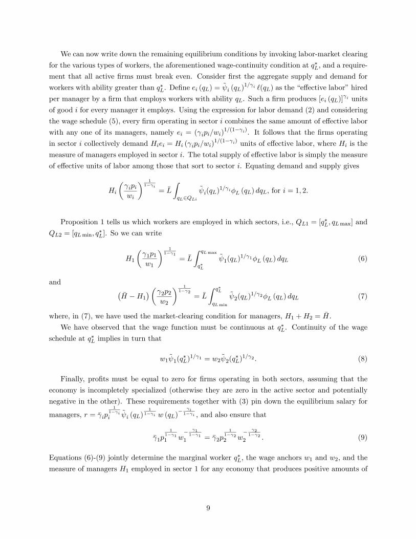
Figure 1 shows the qualitative features of any equilibrium wage schedule. The solid curve depicts
what workers of different abilities actually are paid, considering that those with ability qL ≥ q∗L areemployed in sector 1 and those with ability qL ≤ q∗L are employed in sector 2. The broken curves
show what the workers of different types would be paid if they moved to the opposite sector from
their place of employment, considering that they would only be hired there if firms were indifferent
between employing them and hiring the types that they actually employ in equilibrium. From now
on, we will refer to these wage opportunities in the opposite sector as the “shadow wages.”Notice
that the shadow wages are less than the actual wages, as of course they must be. Notice too that
the worker with the marginal ability q∗L earns the same wage in either of his job opportunities.
We record our observations about the equilibrium sorting pattern in
Proposition 1 Suppose that Assumption 1 holds. Then, in any competitive equilibrium with em-
ployment in both sectors, the more able workers with qL ≥ q∗L are employed in sector 1 and the less
able workers with qL ≤ q∗L are employed in sector 2, for some q∗L ∈ SL.
The intuition for this sorting pattern should be apparent by now. Sorting is determined by
comparing across sectors the ratios εψi/γi. On the one hand, when εψi is large, there is a big
return to moving higher ability workers to sector i inasmuch as marginal ability contributes greatly
to productivity there. On the other hand, when γi is large, output in sector i expands rapidly
with the number of employed workers, irrespective of their ability. In such circumstances, it makes
economic sense to deploy relatively large numbers of workers in the industry. The equilibrium
sorting pattern reflects a trade-off between the returns to ability and the returns to quantity.
8
We can now write down the remaining equilibrium conditions by invoking labor-market clearing
for the various types of workers, the aforementioned wage-continuity condition at q∗L, and a require-
ment that all active firms must break even. Consider first the aggregate supply and demand for
workers with ability greater than q∗L. Define ei (qL) = ψi (qL)1/γi `(qL) as the “effective labor”hired
per manager by a firm that employs workers with ability qL. Such a firm produces [ei (qL)]γi units
of good i for every manager it employs. Using the expression for labor demand (2) and considering
the wage schedule (5), every firm operating in sector i combines the same amount of effective labor
with any one of its managers, namely ei = (γipi/wi)1/(1−γi). It follows that the firms operating
in sector i collectively demand Hiei = Hi (γipi/wi)1/(1−γi) units of effective labor, where Hi is the
measure of managers employed in sector i. The total supply of effective labor is simply the measure
of effective units of labor among those that sort to sector i. Equating demand and supply gives
Hi
(γipiwi
) 11−γi
= L
∫qL∈QLi
ψi(qL)1/γiφL (qL) dqL, for i = 1, 2.
Proposition 1 tells us which workers are employed in which sectors, i.e., QL1 = [q∗L, qLmax] and
QL2 = [qLmin, q∗L]. So we can write
H1
(γ1p1w1
) 11−γ1
= L
∫ qLmax
q∗L
ψ1(qL)1/γ1φL (qL) dqL (6)
and (H −H1
)(γ2p2w2
) 11−γ2
= L
∫ q∗L
qLmin
ψ2(qL)1/γ2φL (qL) dqL (7)
where, in (7), we have used the market-clearing condition for managers, H1 +H2 = H.
We have observed that the wage function must be continuous at q∗L. Continuity of the wage
schedule at q∗L implies in turn that
w1ψ1(q∗L)1/γ1 = w2ψ2(q
∗L)1/γ2 . (8)
Finally, profits must be equal to zero for firms operating in both sectors, assuming that the
economy is incompletely specialized (otherwise they are zero in the active sector and potentially
negative in the other). These requirements together with (3) pin down the equilibrium salary for
managers, r = γip1
1−γii ψi (qL)
11−γi w (qL)
− γi1−γi , and also ensure that
γ1p1
1−γ11 w
− γ11−γ1
1 = γ2p1
1−γ22 w
− γ21−γ2
2 . (9)
Equations (6)-(9) jointly determine the marginal worker q∗L, the wage anchors w1 and w2, and the
measure of managers H1 employed in sector 1 for any economy that produces positive amounts of
9
both goods. The equilibrium salary of managers is given by
r = γip1
1−γii w
− γi1−γi
i , i = 1, 2. (10)
In what follows, we are interested in the determinants of the trade pattern between countries
that differ in their relative endowments of labor to managers and in their distributions of worker
ability. We are also interested in how trade between such countries affects their distributions of
income and measured TFP.
3.1 Determinants of the Trade Pattern
Consider two countries that trade freely at common world prices but that differ in some way in
their factor supplies. Since consumers have identical and homothetic tastes worldwide, the trade
pattern between them can be identified by examining the countries’ relative outputs of the two
goods at the common prices. Accordingly, we investigate how a change in parameters reflecting
factor endowments affects relative outputs of the two goods at given prices.
In each country, a firm in industry i employs ei = (γipi/wi)1/(1−γi) units of effective labor per
manager, thereby producing eγii units of good i. Thus, aggregate output in sector i is
Xi = Hi
(γipiwi
) γi1−γi
, i = 1, 2, (11)
and so
X1X2
=H1(
H −H1) (γ1p1)
γ11−γ1
(γ2p2)γ2
1−γ2
wγ2
1−γ22
wγ1
1−γ11
.
We can substitute the equal-profit condition (9) into this expression to eliminate the wage anchors.
This yields9X1X2
=H1(
H −H1) (1− γ2)p2
(1− γ1)p1,
which implies that the relative output of good 1 is greater in whichever country allocates a greater
share of its managers to producing that good.
3.1.1 Relative Factor Endowments
First, suppose the two countries have the same distributions of worker ability but differ in their
relative aggregate endowments, H/L. To find the pattern of trade, we totally differentiate the
four-equation system comprising (6)-(9) with respect to H/L and examine how a change in relative
endowments affects the allocation of managers to sector 1. The algebra in the appendix establishes
9This condition can alternatively be derived from the observation that in sector i the fraction 1− γi of revenue ispaid to managers, i.e., (1− γi) piXi = rHi.
10
the following proposition.
Proposition 2 Suppose that Assumption 1 holds and that φAL(qL) = φBL (qL) for qL ∈ SAL = SBL .
Then country A exports the manager-intensive good if and only if HA/LA > HB/LB.
Proposition 2 represents, of course, an extension of the Heckscher-Ohlin theorem. When worker
talent is distributed similarly in the two countries, the sorting of workers to sectors generates
no comparative advantages and so has no independent bearing on the trade pattern. Comparative
advantage is governed instead by relative quantities of the factors, just as in the case of homogeneous
labor.
3.1.2 Distributions of Labor Ability
Now suppose that the relative number of managers and workers is the same in the two countries,
but that country A has relatively better workers in the sense that the density function for worker
ability in country A is a rightward shift (RS) of the similar density function in country B. That is,
φBL (qL/λ) = φAL (qL) for all qL ∈ SAL , for some λ > 1, (12)
which has the interpretation that every worker in country A is λ times as productive as his coun-
terpart in the talent distribution in country B. Again, we need to totally differentiate the system
of equations (6)-(9) in order to identify the impact of a rightward shift in the talent distribution on
employment of managers in sector 1. The algebra in the appendix supports the following conclusion.
Proposition 3 Suppose that Assumption 1 holds, that HA/LA = HB/LB, and that φAL (qL) is a
rightward shift of φBL (qL) for some λ > 1. If εψi(q′L) > εψj
(q′′L) for all q′L, q′′L ∈ SAL ∪ SBL , i 6= j,
i, j ∈ {1, 2}, then country A exports good i.
The proposition states that the country that has the superior labor force exports the good
produced in the industry where worker ability contributes more elastically to productivity. Notice
that this need not be the good produced by the country’s most able workers inasmuch as sorting
reflects the ranking of εψ1(qL)/γ1 versus εψ2(qL)/γ2, whereas the trade pattern depends only on
the ranking of εψ1(qL) versus εψ2(qL). This result can be understood by thinking about the sources
of comparative advantage in this setting. With HA/LA = HB/LB, the cross-sectoral difference
in factor intensity is not a source of comparative advantage for either country. Meanwhile, with
εψ1(qL) different from εψ2
(qL), worker ability contributes differently to productivity in the two
sectors. Country A, which is relatively better endowed with more able workers, enjoys a comparative
advantage in the industry in which ability matters more for output.10
10 In the special case in which ψi (qL) is a power function for i = 1, 2, i.e., ψi (qL) = aiqαiL for some ai, αi > 0,
εψi(q′L) > εψj (q
′′L) for all q′L and q
′′L if and only if αi > αj . Moreover, in this case, sL (qL) > 0 for all qL if and only if
α1/γ1 > α2/γ2. Evidently, the conditions of Proposition 3 are easily satisfied. When ψi (qL) is not a power functionfor i = 1, 2, the requirement that εψi(q
′L) > εψj (q
′′L) for all q′L, q
′′L ∈ SAL ∪ SBL , i 6= j, i, j ∈ {1, 2} is not trivial, but
it can be weakened into a comparison of the average elasticities of productivity with respect to ability in the twosectors. See the proof of Proposition 3 in the appendix.
11

We should emphasize, however, that RS puts a great deal of structure on the sense in which
Country A is better endowed with high ability workers than Country B. We might ask, for example,
whether an analogous result to Proposition 3 applies when the distributions of worker talent in the
two countries satisfy the monotone likelihood ratio property (MLRP). The answer is that it does
not. Under MLRP, the country that has the more talented work force will be especially well endowed
with workers that sort to industry 1 even though ability might contribute more to productivity in
industry 2. In such circumstances, the differences in relative supplies of the various qualities could
offset the difference in the contribution of ability to productivity. The structure imposed by RS
ensures that this cannot happen.
3.2 The Effects of Trade on Income Distribution and Measured Productivity
We study next the effect of trade on the income distribution and on measured total factor produc-
tivity (TFP) by examining the comparative statics of the equilibrium with respect to a change in
the relative price of the traded goods.
3.2.1 The Wage Distribution and Managers’Salaries
Suppose that country A exports good 1, the good that is produced with the country’s most able
workers. This might be because the countries have similar distributions of talent but differ in their
relative numbers of workers versus managers, or because the countries have similar relative factor
endowments but differ in their distributions of talent, or for some combination of these reasons.
In any case, we consider the effects on factor returns of an increase in the price of good 1, which
corresponds to an improvement in country A’s terms of trade. When integrated over the range of
prices between the autarky price and the free-trade price, it also reveals the effects in country A of
an opening of international trade.
Note first that the wage function (5) pins down the relative wages of the various workers
employed in either of the two sectors. A small change in the relative price alters the relative pay
only of workers employed in different industries. The calculations in the appendix establish the
following findings.11
Proposition 4 Suppose that Assumption 1 holds. Then when p1 > 0, (i) w1 > w2; (ii) if γ1 ≈ γ2,then w1 > p1 > r > 0 > w2; (iii) if γ1 > γ2 and sL (q∗L) ≈ 0, then w1 ≈ w2 > p1 > 0 > r; and (iv)
if γ1 < γ2 and sL (q∗L) ≈ 0, then r > p1 > 0 > w1 ≈ w2.
Proposition 4 captures the two distinct influences on factor returns in an economy with hetero-
geneous labor. The cross-sectoral difference in factor intensities introduces a force akin to that in
the standard Heckscher-Ohlin model with homogeneous labor, whereby real wages tend to rise and
real managerial salaries tend to fall if the sector experiencing the increase in relative price is the
more labor intensive of the two. But the heterogeneity of labor implies that different workers are
11 In what follows, we use a “hat”over a variable to indicate an incremental, proportional change; i.e., z = dz/z.
12

not equally proficient as potential employees in the two sectors, which introduces a force akin to
that in a specific-factors model (see, e.g., Jones, 1971). Indeed, our result is reminiscent of findings
in a model with “imperfect factor mobility”(Mussa, 1982) or “partially mobile capital”(Grossman,
1983). That is, if the factor intensity differences across industries is large (i.e., γ1 6= γ2) and the
forces for inter-industry sorting of the different worker types are muted (i.e., sL (q∗L) ≈ 0), then
all types of the factor used intensively in sector 1 must gain, while all types of the factor used
intensively in sector 2 must lose (parts (iii) and (iv) of the proposition). On the other hand, if the
factor intensity difference is small (i.e., γ1 ≈ γ2) and the different types of worker are imperfect
substitutes in the two sectors (i.e., sL (qL) > 0), then all workers initially employed in the expand-
ing sector will gain, all workers that continue to be employed in the contracting sector will lose,
and the effect on the well being of managers will depend on their consumption pattern (part (ii) of
the proposition). Finally, note from the wage equation (5) that the relative wages of two workers
with different abilities that are employed in the same sector do not depend on prices. Therefore
an increase in the price of good 1 does not change wage inequality within sectors. Meanwhile, an
increase in the price of good 1 raises the wage anchor in sector 1 relative to the wage anchor in
sector 2 (see part (i) of the proposition). And since the higher-ability, higher-wage workers are
employed in sector 1, this implies that by raising wages in sector 1 relative to wages in sector 2 an
increase in the price of good 1 increases overall wage inequality, while reducing wage inequality in
the other country.
3.2.2 Measured TFP
In our setting, trade affects productivity by altering the composition of factors employed in each
industry. Of course, if factor heterogeneity were properly taken into account in any measurement
exercise, there could be no productivity gains or losses here inasmuch as all firms in an industry
use the same production technology and technologies do not change as a result of trade. But
productivity measures often do not account for fine differences in worker or managerial ability.
Rather, they consider productivity gains as a residual after accounting for changes in output that
can be associated with changes in input quantities in broad factor categories. Accordingly, it seems
interesting to ask what our model has to say about the effects of trade on measured TFP when we
take a stylized representation of the way that productivity typically is measured.
With our specification of the production functions, output in each industry is a Cobb-Douglas
function of the quantities of capital and labor, with productivity determined by the abilities of the
workers employed there. Let us write aggregate output in sector i as
Xi = AiLγii H
1−γii ,
where Li = L∫qL∈QLi φL (qL) dqL is the aggregate employment of labor in sector i and Hi =
L∫qL∈QLi [φ (qL) /` (qL)] dqL is the aggregate number of managers hired there. We can view Ai as
a measure of TFP in industry i when the abilities of different workers are not observed by the
13

analyst. This measure of productivity is close to what is used in most empirical studies. We ask,
how does trade affect Ai?
When the relative price of good 1 increases, additional workers are drawn to industry 1. The
marginal workers that join the sector are less productive than those employed there beforehand,
since sL (qL) > 0 implies that the the industry initially attracts all workers with ability above
the threshold, q∗L. Firms match these marginal workers with appropriate numbers of homogeneous
managers. It follows that measured TFP in industry 1 falls. Meanwhile, industry 2 sheds its most
able workers. So measured TFP in that sector falls as well. In short, the country that exports
good 1 sees a fall in measured productivity in both sectors as the result of an opening of trade or
after any increase in the price of its export good. Just the opposite is true in the other country,
where an expansion of the export sector means that the marginal workers are more talented than
any who were previously employed there and the contraction of the import-competing sector means
that this sector loses its least able workers.
Formally, we show in the appendix that
A1/γ11 = E
[ψ1(qL)1/γ1 | qL ≥ q∗L
]and
A1/γ22 = E
[ψ2(qL)1/γ2 | qL ≤ q∗L
],
where E is the expectations operator. Apparently, both A1 and A2 are increasing functions of q∗L.As p1 increases and sector 1 expands, the ability of the marginal worker q∗L declines in the country
that exports good 1 and measured TFP falls in both sectors. The opposite is true in the country
that imports good 1; as p1 declines there, q∗L grows, and measured TFP rises in both sectors. We
have therefore established
Proposition 5 Suppose that Assumption 1 holds. Then international trade reduces measured TFPin both sectors in the country that exports good 1 and raises measured TFP in both sectors in the
country that imports this good.
Here, trade has opposite implications for measured productivity in the two countries. If, for
example, the country that has a comparative advantage in good 1 also has access to superior
technologies for producing the two goods, then the opening of trade will generate a convergence in
measured TFP. Such convergence would reflect only the induced changes in factor composition in
the various sectors and not any international diffusion of technology.
3.3 Sorting Reversal
So far, we have used Assumption 1 to characterize the sorting of heterogeneous workers and the
resulting trade structure. In this final part of the section on homogeneous managers we clarify
what can happen when sL (qL) switches sign.
14

0.5 1 1.5 2 2.50.1
0.15
0.2
0.25
0.3
0.35
0.4
0.45
0.5
0.55
0.6
qL
w(q
L)
Sector 1 wagesSector 2 wagesSector 1 shadow wagesSector 2 shadow wages
Figure 2: Wages with a reversal of sorting
First note that if ψi (qL) is a power function for i = 1, 2, the function sL (qL) does not depend
on qL inasmuch as the elasticities of productivity with respect to ability then are constants. In such
circumstances, sL (qL) is either always positive or always negative, and we can assume sL (qL) > 0
without loss of generality, because this only amounts to a particular labeling of the sectors. However,
when ψi (qL) is not a power function for some i, the assumption that sL (qL) has a uniform sign
for all qL ∈ SL imposes meaningful restrictions on the forms of the productivity functions and thesupport of the distribution of worker talent. Without these restrictions, we cannot be sure that the
most able workers sort into one sector and the least able workers sort into the other.
To illustrate what can happen when sL (qL) changes signs, suppose that the productivity of a
firm in sector i that hires workers of ability qL is given by
ψi (qL) =(αiq
ρiL + 1
)1/ρi , αi > 0, ρi < 0 for i = 1, 2. (13)
This specification implies a constant elasticity of substitution between the ability of workers and
the ability of managers in generating the productivity of the firm, and that worker and managerial
ability are, in fact, complements. Of course, with homogeneous managers, firms have no possibility
to adjust manager type in order to take advantage of this complementarity. Nonetheless, the CES
specification for productivity represents a legitimate and even a plausible functional form.
When productivity takes the form indicated in (13), the elasticity of productivity with respect to
worker ability in sector i is given by εψi (qL) = αiqρiL /(αiq
ρiL + 1
). If ρ1 6= ρ2 then εψ1 (qL)−εψ2 (qL)
necessarily switches signs on qL ∈ [0,+∞) and therefore sL (qL) may switch signs on the support
of the distribution of worker ability, depending on the industry factor intensities and the range of
the talent distribution.
Figure 2 depicts an equilibrium wage schedule for an economy in which sL (qL) < 0 for low
values of qL and sL (qL) > 0 for high values of qL.12 In this economy, the most and least able
workers sort to sector 1 while a middle range of workers is hired into sector 2. The thin solid curves
12See Lim (2013) for the functional forms and parameter values that were used to generate this figure.
15
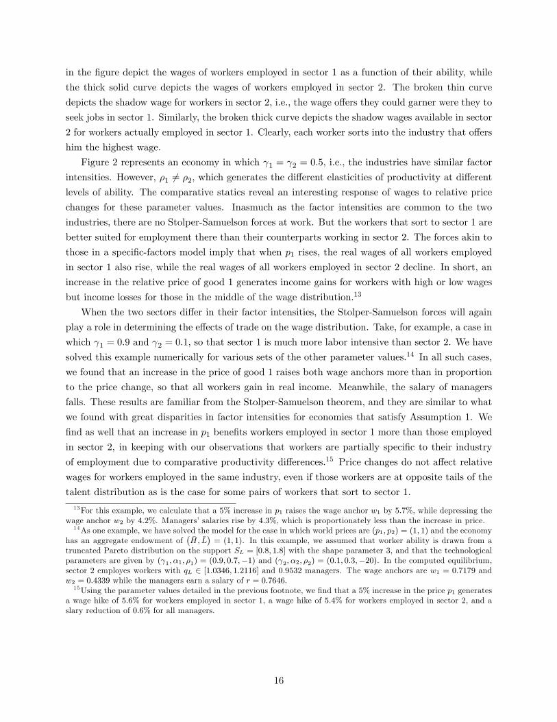
in the figure depict the wages of workers employed in sector 1 as a function of their ability, while
the thick solid curve depicts the wages of workers employed in sector 2. The broken thin curve
depicts the shadow wage for workers in sector 2, i.e., the wage offers they could garner were they to
seek jobs in sector 1. Similarly, the broken thick curve depicts the shadow wages available in sector
2 for workers actually employed in sector 1. Clearly, each worker sorts into the industry that offers
him the highest wage.
Figure 2 represents an economy in which γ1 = γ2 = 0.5, i.e., the industries have similar factor
intensities. However, ρ1 6= ρ2, which generates the different elasticities of productivity at different
levels of ability. The comparative statics reveal an interesting response of wages to relative price
changes for these parameter values. Inasmuch as the factor intensities are common to the two
industries, there are no Stolper-Samuelson forces at work. But the workers that sort to sector 1 are
better suited for employment there than their counterparts working in sector 2. The forces akin to
those in a specific-factors model imply that when p1 rises, the real wages of all workers employed
in sector 1 also rise, while the real wages of all workers employed in sector 2 decline. In short, an
increase in the relative price of good 1 generates income gains for workers with high or low wages
but income losses for those in the middle of the wage distribution.13
When the two sectors differ in their factor intensities, the Stolper-Samuelson forces will again
play a role in determining the effects of trade on the wage distribution. Take, for example, a case in
which γ1 = 0.9 and γ2 = 0.1, so that sector 1 is much more labor intensive than sector 2. We have
solved this example numerically for various sets of the other parameter values.14 In all such cases,
we found that an increase in the price of good 1 raises both wage anchors more than in proportion
to the price change, so that all workers gain in real income. Meanwhile, the salary of managers
falls. These results are familiar from the Stolper-Samuelson theorem, and they are similar to what
we found with great disparities in factor intensities for economies that satisfy Assumption 1. We
find as well that an increase in p1 benefits workers employed in sector 1 more than those employed
in sector 2, in keeping with our observations that workers are partially specific to their industry
of employment due to comparative productivity differences.15 Price changes do not affect relative
wages for workers employed in the same industry, even if those workers are at opposite tails of the
talent distribution as is the case for some pairs of workers that sort to sector 1.
13For this example, we calculate that a 5% increase in p1 raises the wage anchor w1 by 5.7%, while depressing thewage anchor w2 by 4.2%. Managers’salaries rise by 4.3%, which is proportionately less than the increase in price.14As one example, we have solved the model for the case in which world prices are (p1, p2) = (1, 1) and the economy
has an aggregate endowment of(H, L
)= (1, 1). In this example, we assumed that worker ability is drawn from a
truncated Pareto distribution on the support SL = [0.8, 1.8] with the shape parameter 3, and that the technologicalparameters are given by (γ1, α1, ρ1) = (0.9, 0.7,−1) and (γ2, α2, ρ2) = (0.1, 0.3,−20). In the computed equilibrium,sector 2 employes workers with qL ∈ [1.0346, 1.2116] and 0.9532 managers. The wage anchors are w1 = 0.7179 andw2 = 0.4339 while the managers earn a salary of r = 0.7646.15Using the parameter values detailed in the previous footnote, we find that a 5% increase in the price p1 generates
a wage hike of 5.6% for workers employed in sector 1, a wage hike of 5.4% for workers employed in sector 2, and aslary reduction of 0.6% for all managers.
16

4 Heterogeneous Managers with Cobb-Douglas Productivity
We now introduce manager heterogeneity. We begin with a special case in which managerial ability
and worker ability make multiplicatively separable contributions to the productivity of the unit and
take a Cobb-Douglas (i.e., constant elasticity) form. In particular, we shall assume in this section
that
ψi (qH , qL) = qβiH q
αiL for i = 1, 2; αi, βi > 0. (14)
Note that, in this case, productivity is a weakly log supermodular function of the two ability levels.
As such, the complementarity between the talent of workers and that of the manager is somewhat
muted compared to what arises with strict log supermodularity, which means the forces for positive
assortative matching within a sector are correspondingly weaker. The Cobb-Douglas case is simpler
to analyze than the case with stronger complementarities, so we postpone the latter in order to
shed light on some of the economic forces at works.
In this section and what follows, we model the diversity of manager types in parallel to that
for workers. In particular, there is a mass Hc of managers in country c and a probability density
φcH (qH) of managers with ability qH for qH ∈ ScH = [qcHmin, qcHmax]. We take the supply of managers
and their ability distribution as given throughout the analysis.
There is no need to go through all the steps of a firm’s profit maximization problem, because
the derivation proceeds much as for the case with homogeneous managers in Section 3. Suffi ce it to
say that the demand per manager for workers of ability qL by a firm in industry i that pairs these
workers with a manager of ability qH is given by
` (qL, qH) =
[γipiq
βiH q
αiL
w (qL)
] 11−γi
. (15)
Substituting (15) into the expression for profits yields
πi (qL, qH) = γip1
1−γii
(qβiH q
αiL
) 11−γi w (qL)
− γi1−γi − r (qH) , (16)
where r(qH) is the salary of a manager with ability qH and γi ≡ γγi
1−γii (1− γi). Every firm chooses
the ability of its workers and the ability of its manager so as to maximize profits, yet free entry
dictates that these profits must be equal to zero in equilibrium. Let Mi be the set of all matches
that maximize profits in sector i. For each pairing (qL, qH) in Mi,
r (qH) = γip1
1−γii
(qβiH q
αiL
) 11−γi w (qL)
− γi1−γi , i = 1, 2, (17)
by dint of the zero-profit condition. Profit maximization with respect to the choice of types, evalu-
17
ated for pairings that achieve zero profits in accordance with (17), yields the first-order conditions,
αiγi
= ew(qL) for qL ∈ QintLi (18)
andβi
1− γi= er(qH) for qH ∈ QintHi . (19)
Equation (18) is the analog to (4) and equates the ratio of the elasticities of output with respect
to worker ability and labor quantity to the elasticity of the wage schedule. Equation (19) has a
similar interpretation regarding a firm’s choice of manager type.
In equilibrium, all worker types must be employed, which means that firms in some sector (or
both) must demand the full range of workers. Equation (18) can be satisfied for a range of workers
only if the wage schedule has a constant elasticity over this range. Therefore, the equilibrium wage
schedule must take the form
w (qL) = wiqαi/γiL for qL ∈ QintLi . (20)
The salary schedule for managers must have a similar form, namely
r (qH) = riqβi/(1−γi)H for qH ∈ QintHi , (21)
where ri is a “salary anchor”analogous to wi.
When the wage function has a constant elasticity equal to αi/γi for a range of worker types, a
firm in sector i is indifferent as to its choice of employees among workers in this range, irrespective of
the ability of its manager. And when the salary function has an elasticity equal to βi/ (1− γi), thefirm is indifferent to the ability of its managers. Accordingly, the matching of workers and managers
among those that sort to sector i is indeterminate in the Cobb-Douglas case. This indeterminacy
reflects the fact that the productivity function in (14) is only weakly log supermodular and thus
provides no clear incentives for positive (or negative) assortative matching.
Although the matching of workers and managers in a sector is not determined in the Cobb-
Douglas case, the sorting of these factors to the two sectors follows a familiar pattern. The elasticity
of the wage schedule must be greater along its upper segment than along its lower segment, or else
firms that hire the less able workers would all prefer to upgrade their employees. Similarly, the
elasticity of the salary schedule must be greater along its upper segment than its lower segment. We
designate as sector 1 whichever industry has the greater ratio of the output elasticity with respect to
worker ability to the output elasticity with respect to labor quantity. With this labeling convention,
sL = α1/γ1−α2/γ2 > 0. Then, in any equilibrium in which a country produces both goods, sector
1 attracts the workers with ability qL above some cutoff q∗L. If sH = β1/ (1− γ1)−β2/ (1− γ2) > 0,
then sector 1 also attracts the more able managers with qH > q∗H ; otherwise, the sorting of managers
is opposite to that for workers.
For precision, we state more formally the environment we consider throughout this section and
the sorting pattern that results.
18

Assumption 2 (i) SH = [qHmin, qHmax], 0 < qHmin < qHmax < +∞; (ii) ψi (qH , qL) = qβiH q
αiL ,
αi, βi > 0, for i = 1, 2; and (iii) sL ≡ α1/γ1 − α2/γ2 > 0.
Proposition 6 Suppose that Assumption 2 holds. Then, in any competitive equilibrium with em-
ployment in both sectors, the more able workers with qL ≥ q∗L are employed in sector 1 and the less
able workers with qL ≤ q∗L are employed in sector 2, for some q∗L ∈ SL. If sH > 0 (sH < 0), the
more able managers with qH ≥ q∗H are employed in sector 1 (sector 2) and the less able managers
with qH ≤ q∗H are employed in sector 2 (sector 1), for some q∗H ∈ SH .
To describe the equilibrium once the sorting pattern has been settled, we invoke factor-market
clearing, continuity of worker wages, continuity of managerial salaries, and the zero-profit condi-
tions. For concreteness, let us focus on the case in which sH > 0 so that the more able managers
sort to industry 1; the opposite case can be handled similarly.
It proves convenient to define eHi (qH) = qβi/(1−γi)H as the effective managerial input of a manager
with ability qH who works in sector i. Then the aggregate supplies of effective managerial input in
sectors 1 and 2 are
H1 = H
∫ qHmax
q∗H
qβ1
1−γ1H φH (qH) dqH , (22)
and
H2 = H
∫ q∗H
qHmin
qβ2
1−γ2H φH (qH) dqH , (23)
respectively. Note that H1/H depends only on q∗H and is a monotonically decreasing function, and
H2/H also depends only on q∗H and is monotonically increasing.
Consider now the supply and demand for effective labor in sector 1, where we define eLi (qL) =
qαi/γiL as the effective labor provided by a worker of ability qL in sector i. From the labor demand
equation (15), a firm in sector 1 combines a manager with eHi units of effective managerial input
with eHi (γipi/wi)1/(1−γi) units of effective labor. Therefore, the H1 units of effective managerial
input that are hired into sector 1 are combined with H1 (γ1p1/w1)1/(1−γ1) units of effective labor.
Noting the definition of H1 and equating the demand for effective labor in sector 1 with the supply
of effective labor among those with ability above q∗L, we have
H
(γ1p1w1
) 11−γ1
∫ qHmax
q∗H
qβ1
1−γ1H φH (qH) dqH = L
∫ qLmax
q∗L
qα1γ1L φLdqL. (24)
A similar condition applies in sector 2, where labor-market clearing requires
H
(γ2p2w2
) 11−γ2
∫ q∗H
qHmin
qβ2
1−γ2H φH (qH) dqH = L
∫ q∗L
qLmin
qα2γ2L φLdqL. (25)
Continuity of the wage schedule at q∗L requires that
w1 (q∗L)α1γ1 = w2 (q∗L)
α2γ2 . (26)
19
The salary function for managers must also be continuous and firms that hire managers with ability
q∗H must earn zero profits in either sector. Together, these considerations imply
γ1p1
1−γ11 w
− γ11−γ1
1 (q∗H)β1
1−γ1 = γ2p1
1−γ22 w
− γ21−γ2
2 (q∗H)β2
1−γ2 . (27)
Equations (24)-(27) comprise four equations that can be used to solve for the two wage anchors,
w1 and w2, and the two cutoffs, q∗L and q∗H . The effective supply of managers in sectors 1 and 2,
H1 and H2, can then be solved from (22) and (23). Finally, the salary anchors for the managers
can be computed from the zero-profit conditions, which imply
ri = γip1
1−γii w
− γi1−γi
i for i = 1, 2. (28)
This completes our characterization of the supply-side equilibrium for an economy that faces prices
p1 and p2.
4.1 Pattern of Trade
As before, we need an expression for an economy’s relative outputs in order to conduct the compar-
ative static analysis that reveals the pattern of trade between countries that differ in their relative
factor endowments or in their distributions of factor types. The Hi units of effective managers
employed in sector i collectively produce Xi = Hi (γipi)γi/(1−γi)w
−γi/(1−γi)i units of good i. Each
effective unit of managerial input is paid a salary of ri in sector i and– by continuity of the salary
function– r1/r2 = (q∗H)−sH (see (21)). Using this condition together with (24)-(25) and (27)-(28),
we can write
X1X2
=r1H1r2H2
(1− γ2) p2(1− γ1) p1
(29)
=(1− γ2) p2
∫ qHmax
q∗Hq
β11−γ1H φH (qH) dqH
(1− γ1) p1∫ q∗HqHmin
qβ2
1−γ2H φH (qH) dqH
(q∗H)−sH .
Similar to the case of homogeneous managers, the first line of (29) reflects the fact that the aggregate
salaries of all managers in sector i absorb a fraction 1− γi of revenue. And the second line impliesthat, since sH > 0 in the case under consideration, X1/X2 is a decreasing function of q∗H . Therefore,
to identify the pattern of trade, we need only find which country allocates more effective managerial
input to sector 1 relative to its aggregate endowment of managers; that is, how q∗H varies with factor
endowments.16
The system of equations (24)-(27) that applies with Cobb-Douglas productivity is quite similar
to the system (6)-(9) that applies when managers are homogeneous, except that now we need
16Note that in the opposite case, when sH < 0, managers with qH ≥ q∗H sort into sector 2 while managers withqH ≤ q∗H sort into sector 1. As a result, X1/X2 is an increasing function of q∗H .
20
to use the effective managerial input in a sector in place of the pure number of managers. In
other words, the multiplicative separability of the productivity function allows us to construct an
aggregate measure of managerial input that plays the same role as does the number of managers
when managers are equally productive. We can do so, because there are no forces present in the
Cobb-Douglas case to induce any particular pattern of matching within either sector. It stands
to reason that the determinants of the trade pattern with heterogeneous managers but Cobb-
Douglas productivity are analogous to those we found for the case of homogeneous managers. In
the appendix, we prove
Proposition 7 Suppose that Assumption 2 holds. Then if φAL(qL) = φBL (qL) for all qL ∈ SAL = SBL ,
φAH(qH) = φBH (qH) for all qH ∈ SAH = SBH , and HA/LA > HB/LB, country A exports the manager-
intensive good.
Proposition 8 Suppose that Assumption 2 holds and HA/LA = HB/LB. Then, (i) if φAH(qH) =
φBH (qH) for all qH ∈ SAH = SBH and φAL (qL) is a rightward shift of φBL (qL) for some λ > 1, then
country A exports good 1 if and only if α1 > α2; (ii) if φAL(qL) = φBL (qL) for all qL ∈ SAL = SBL and
φAH(qH) is a rightward shift of φBH (qH) for some λ > 1, then country A exports good 1 if and only
if β1 > β2.
In short, the Heckscher-Ohlin theorem applies when countries have similar distributions of factor
types but differ in their relative aggregate endowments of managers versus workers. Alternatively, if
the relative factor endowments are the same in the two countries but they differ in their distributions
of one of the factors, then the country with the rightward-shifted distribution of a factor exports
the good produced by the industry in which productivity responds more elastically to that factor’s
ability.
4.2 Effects of Trade on Income Distribution and Measured Productivity
Our results on income distribution also carry over straightforwardly from the case with homo-
geneous managers to that with manager heterogeneity but Cobb-Douglas productivity. First
note that within-industry income distribution is not affected by world trade inasmuch as the
elasticity of the wage schedule for workers employed in a given industry is constant. As a re-
sult, (20) implies that w (q′L) /w (q′′L) = (q′L/q′′L)αi/γi for q′L, q
′′L ∈ QLi and (21) implies that
r (q′H) /r (q′′H) = (q′H/q′′H)βi/(1−γi) for q′H , q
′′H ∈ QHi. Second, relative rewards of workers and
managers that are employed in different industries do change with trade, inasmuch as the wage and
salary anchors wi and ri change. In the appendix we prove
Proposition 9 Suppose that Assumption 2 holds and sH ≈ 0. When p1 > 0, (i) w1 > w2; (ii) if
γ1 ≈ γ2, then w1 > p1 > r1 ≈ r2 > 0 > w2; (iii) if γ1 > γ2 and sL ≈ 0, then w1 ≈ w2 > p1 > 0 >
r1 ≈ r2; (iv) if γ1 < γ2 and sL ≈ 0, then r1 ≈ r2 > p1 > 0 > w1 ≈ w2.
21

Proposition 9 can be understood by recognizing that the model with heterogeneous workers
and managers contains a blend of Stolper-Samuelson and Ricardo-Viner forces. When sH ≈ 0,
there is no difference in the suitability of the various managers for employment in one sector versus
the other, because the comparative advantage associated with greater ability of the input just
offsets the comparative advantage associated with greater quantity. Then, it is as if managers are
a perfectly mobile, homogeneous factor. When sL also is small, the Stolper-Samuelson forces will
dominate, and workers in both industries will see a gain in real income if the relative price of the
labor-intensive good rises and will see a loss in real income if the relative price of the labor-intensive
good falls. In contrast, if factor intensities are approximately the same in the two industries, the
Stolper-Samuelson forces will be muted, and the partial specificity of workers arising from the
comparative advantage of ability in sector 1 will govern the income responses. Then, workers will
benefit in real terms when the relative price of the good they produce rises and will lose in real
terms if the relative price of this good falls. Also note that similar considerations imply that if
sH > 0 but sL ≈ 0 and γ1 ≈ γ2, the economy behaves like one with sector-specific managers and
perfectly mobile labor. Then r1 > p1 > w1 ≈ w2 > 0 > r2, i.e., managers in the expanding sector
gain, managers in the contracting sector lose, and workers may gain or lose in real terms depending
on their consumption pattern. Finally, similarly to Proposition 4, an increase in the price of good
1 raises overall wage inequality, because it does not change relative wages within sectors and it
increases wages of the more able, better-paid workers employed in sector 1 relative to the less able,
lower-paid workers in sector 2.
Turning to the effects of trade on measured productivity, our conclusions also are reminiscent
of those we have seen before. Recalling that
Xi = H
(γipiwi
) γi1−γi
∫qH∈QHi
qβi/(1−γi)H φH (qH) dqH , for i = 1, 2,
we can substitute the labor market clearing conditions (24) and (25) to write output in sector i as
Xi = LγiH1−γi(∫
qL∈QLiqαi/γiL φL (qL) dqL
)γi (∫qH∈QHi
qβi/(1−γi)H φH (qH) dqH
)1−γi.
Since the aggregate factor inputs in sector i are Li = L∫qL∈QLi φL (qL) dqL and Hi =
H∫qH∈QHi φH (qH) dqH , we can write measured TFP as
Ai =
(∫qL∈QLi q
αi/γiL φL (qL) dqL
)γi (∫qH∈QHi q
βi/(1−γi)H φH (qH) dqH
)1−γi(∫qL∈QLi φL (qL) dqL
)γi (∫qH∈QHi φH (qH) dqH
)1−γi=
(E[qαi/γiL | qL ∈ QLi
])γi (E[qβi/(1−γi)H | qH ∈ QHi
])1−γi.
Now take the case in which sH > 0. Then an increase in p1 causes sector 1 to expand by
attracting both more workers and more managers; i.e., both q∗L and q∗H decline. The movement
22
of marginal factors from sector 2 to sector 1 reduces the average ability of both factors in both
industries. As a result, measured productivity falls in both sectors. However, if sH < 0, sector 1
attracts the best workers but the worst managers. As this sector expands, average worker ability
declines but average manager ability grows. In this case, TFP can rise or fall in either industry
and possibly can move in opposite directions in the two industries.
5 Strong Complementarities between Heterogeneous Factors
The Cobb-Douglas case is special, because when alternative worker teams are paired with a given
manager, their relative productivity is independent of the ability of that manager.17 In such cir-
cumstances, the matching of workers and managers is not determined by the requirements for a
competitive equilibrium. We depart now from multiplicative separability in order to study produc-
tivity functions that induce a determinate pattern of matching in each industry. In particular, we
adopt
Assumption 3 (i) SH = [qHmin, qHmax], 0 < qHmin < qHmax < +∞; (ii) ψi (qH , qL) is strictly
increasing, twice continuously differentiable, and strictly log supermodular for i = 1, 2.
This assumption implies that ψiH (qH , qL) /ψi (qH , qL) is increasing in qL and ψiL (qH , qL) /ψi (qH , qL)
is increasing in qH , where ψiF (qH , qL) is the partial derivative of ψi (qH , qL) with respect to qF ,
F = H,L.
Proceeding as before, we first find the labor demand per manager by a firm in sector i, taking
as given the common ability of the team of workers and the ability of the manager. We substitute
the optimal labor demand ` (qH , qL) into the expression for profits to derive the profit function,
πi (qH , qL) = γip1
1−γii ψi (qH , qL)
11−γi w (qL)
− γi1−γi − r (qH) . (30)
Each firm chooses the ability of its workers and the ability of its manager so as to maximize profits
taking the wage and salary schedules as given, while free entry dictates that realized profits for
active firms are zero. The wage schedule w (qL) is continuous and strictly increasing for all qL ∈ SLand the salary schedule r (qH) is continuous and strictly increasing for all qH ∈ SH .18
We solve the firm’s profit-maximization problem in two stages. First, given qH , the firm chooses
the most suitable workers, deriving thereby the profits
Πi (qH) = maxqL∈SL
πi (qH , qL) , for qH ∈ SH , i = 1, 2. (31)
17 In fact, this property is shared by any productivity function that is multiplicatively separable in the ability levelsof the two factors.18The productivity function ψi (·) is strictly increasing for i = 1, 2. Therefore if w (·) were discontinuous at some
qL, then there would be no demand for workers with abilities just above or just below qL. Moreover, if the wagefunction were not strictly increasing, there would be no demand for some positive measure of workers. If, for example,w (·) were flat or declining over some interval beginning at qL, there would be no demand for workers in an intervalbounded below by qL. Analogous arguments apply to the salary schedule r (·).
23
Second, it chooses qH to maximize Πi (qH). We show in the appendix that the solution to this
problem results in equilibrium allocation sets QLi and QHi that must be unions of closed intervals,
where QFi is the set of types of factor F that sorts to industry i, for F = H,L and i = 1, 2.
Moreover, there is positive assortative matching (PAM) within each sector; that is, in each industry
the better workers are matched with the better managers (see Eeckhout and Kircher, 2012). It canhappen, however, that when comparing a more able manager employed in sector 2 and a less able
manager employed in sector 1, the latter oversees better workers than the former. In other words,
PAM may fail across sectors, as we shall see in several examples below.
Let mi (qH) denote the solution to (31). Then
m (qH) =
{m1 (qH) for qH ∈ QH1m2 (qH) for qH ∈ QH2
.
The equilibrium pairings in sector i are
Mi = [{qH , qL} | qL ∈ mi (qH) for all qH ∈ QHi] ,
where Mi is a closed graph consisting of a union of connected sets Mni such that mi (qH) is contin-
uous and strictly increasing in each set but may jump discontinuously between them.
Now consider an equilibrium with incomplete specialization, so that both QH1 and QH2 are of
positive measure. Then Πi (qH) = 0 for all qH ∈ QHi, i = 1, 2, which implies
r (qH) = γip1
1−γii ψi [qH ,mi (qH)]
11−γi w [mi (qH)]
− γi1−γi for all qH ∈ QHi, i = 1, 2. (32)
Continuity of the wage and salary schedules implies that both functions are differentiable almost
everywhere. Moreover, profit maximization and (32) imply that, at all interior points of a connected
subset Mni of Mi, the salary function r (·) and the wage function w (·) are differentiable; see the
appendix for proof. It follows that the solution to (31) must satisfy the first-order condition
m (qH)ψiL [qH ,m (qH)]
γiψi [qH ,m (qH)]= εw(m(qH)) for all {qH ,m (qH)} ∈Mn,int
i , n ∈ Ni, i = 1, 2, (33)
where Mn,inti is the interior of Mn
i . Also, (32) and (33) imply that
qHψiH [qH ,m (qH)]
(1− γi)ψi [qH ,m (qH)]= εr(qH) for all {qH ,m (qH)} ∈Mn,int
i , n ∈ Ni, i = 1, 2. (34)
Note the similarity between these equations and (18) and (19), which apply in the Cobb-Douglas
case. The difference is that now the elasticities of productivity with respect to a factor’s ability
depend on the worker-manager combinations that occur in equilibrium.
It remains to describe the sorting conditions at boundary points between some Mn1 and some
Mn′2 . Let q
†L be some such boundary point, so that workers with ability just above q
†L sort to one
24

sector while workers with ability just below q†L sort to the other. For this, we require the wage
function w (qL) to be at least as steep to the right of q†L as to the left; otherwise the firms that
employ workers with abilities just below q†L could earn positive profits by hiring slightly more able
workers and likewise firms that hire workers with abilities above q†L could earn profits by hiring
slightly less able workers. By a similar argument, the salary function r (qH) must be (weakly)
steeper just to the right of any boundary point q†H than just to the left of such a point.
We turn next to the factor-market clearing conditions. To this end, define QHi (qH) as the
set of all managers that sort to sector i whose ability does not exceed qH . Similarly, define
QLi (qL) as the set of workers that sort to sector i whose ability does not exceed qL. A profit-
maximizing firm in sector i that hires workers of ability qL and managers of ability qH demands
` (qH , qL) = [γir (qH)] / [(1− γi)w (qL)] workers per manager. Since the matching function is every-
where increasing, it follows that
H
∫q∈QHi(qminHi )
γir (q)
(1− γi)w [m (q)]φH (q) dq + H
∫ qH
qminHi
γir (q)
(1− γi)w [m (q)]φH (q) dq
= L
∫q∈QLi[m(qminHi )]
φL (q) dq + L
∫ m(qH)
m(qminHi )φL (q) dq for all qH ∈
(qminHi , q
maxHi
), i = 1, 2,
where the left-hand side represents the labor demanded by all firms in sector i hiring managers
with ability not exceeding qH and the right-hand side represents the measure of workers available
to be teamed with those managers. Since the left-hand side is differentiable in qH , this equation
implies that the matching functionm (qH) also is differentiable at points in(qminHi , q
maxHi
). That being
the case, we can differentiate the labor-market clearing condition with respect to qH to derive a
differential equation for the matching function, namely
Hγir (qH)
(1− γi)w [m (qH)]φH (qH) = LφL [m (qH)]m′ (qH) (35)
for {qH ,m (qH)} ∈ Mn,inti , n ∈ Ni, i = 1, 2.
Equations (33), (34) and (35) comprise three differential equations that are satisfied in any
competitive equilibrium by the wage schedule w (qL), the salary schedule r (qH), and the matching
function m (qH). Together with the zero-profit condition and a set of boundary conditions, these
equations can be used to characterize an equilibrium allocation.
Let us consider first the possibility that the set of workers that sorts to each sector comprises
a single, connected interval, and similarly for managers. That is, we consider equilibria that are
characterized by two thresholds, q∗L and q∗H , such that all workers with ability less than q
∗L sort to
some sector while all workers with ability greater than q∗L sort to the other, and all managers with
ability less than q∗H sort to some sector while all managers with ability greater than q∗H sort to the
other. Note that we do not insist that the better workers and better managers sort to the same
sector, nor do we claim that all competitive equilibria are characterized by such a simple sorting
pattern.
25
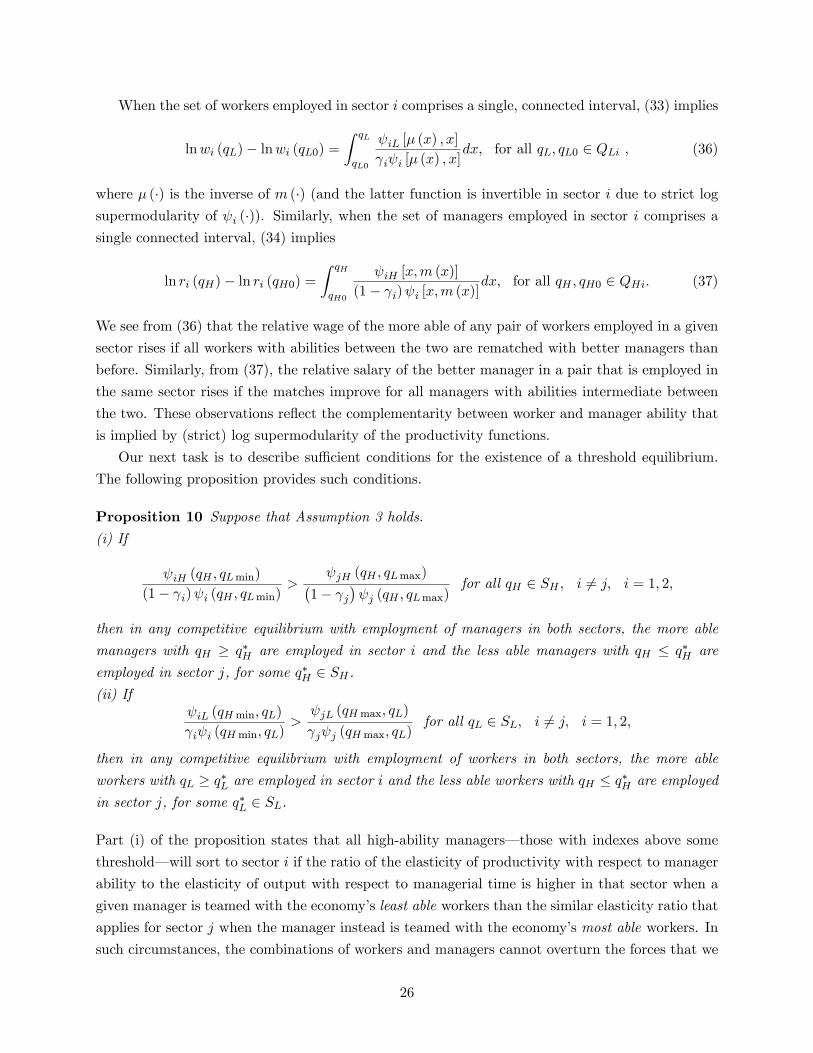
When the set of workers employed in sector i comprises a single, connected interval, (33) implies
lnwi (qL)− lnwi (qL0) =
∫ qL
qL0
ψiL [µ (x) , x]
γiψi [µ (x) , x]dx, for all qL, qL0 ∈ QLi , (36)
where µ (·) is the inverse of m (·) (and the latter function is invertible in sector i due to strict logsupermodularity of ψi (·)). Similarly, when the set of managers employed in sector i comprises asingle connected interval, (34) implies
ln ri (qH)− ln ri (qH0) =
∫ qH
qH0
ψiH [x,m (x)]
(1− γi)ψi [x,m (x)]dx, for all qH , qH0 ∈ QHi. (37)
We see from (36) that the relative wage of the more able of any pair of workers employed in a given
sector rises if all workers with abilities between the two are rematched with better managers than
before. Similarly, from (37), the relative salary of the better manager in a pair that is employed in
the same sector rises if the matches improve for all managers with abilities intermediate between
the two. These observations reflect the complementarity between worker and manager ability that
is implied by (strict) log supermodularity of the productivity functions.
Our next task is to describe suffi cient conditions for the existence of a threshold equilibrium.
The following proposition provides such conditions.
Proposition 10 Suppose that Assumption 3 holds.(i) If
ψiH (qH , qLmin)
(1− γi)ψi (qH , qLmin)>
ψjH (qH , qLmax)(1− γj
)ψj (qH , qLmax)
for all qH ∈ SH , i 6= j, i = 1, 2,
then in any competitive equilibrium with employment of managers in both sectors, the more able
managers with qH ≥ q∗H are employed in sector i and the less able managers with qH ≤ q∗H are
employed in sector j, for some q∗H ∈ SH .(ii) If
ψiL (qHmin, qL)
γiψi (qHmin, qL)>
ψjL (qHmax, qL)
γjψj (qHmax, qL)for all qL ∈ SL, i 6= j, i = 1, 2,
then in any competitive equilibrium with employment of workers in both sectors, the more able
workers with qL ≥ q∗L are employed in sector i and the less able workers with qH ≤ q∗H are employedin sector j, for some q∗L ∈ SL.
Part (i) of the proposition states that all high-ability managers– those with indexes above some
threshold– will sort to sector i if the ratio of the elasticity of productivity with respect to manager
ability to the elasticity of output with respect to managerial time is higher in that sector when a
given manager is teamed with the economy’s least able workers than the similar elasticity ratio that
applies for sector j when the manager instead is teamed with the economy’s most able workers. In
such circumstances, the combinations of workers and managers cannot overturn the forces that we
26

have previously identified that indicate sorting of the best managers to sector i.19 Part (ii) of the
proposition has a similar interpretation for labor sorting; the condition ensures that the ranking of
sectors by elasticity ratio cannot be overturned even after allowing for the workers’most favorable
pairing in one sector compared to their least favorable pairing in the other.
If the conditions for Proposition 10 are satisfied, then the top tier of managers sorts to some
sector as does the top tier of workers, although the sector chosen by the best workers need not be
the same as that chosen by the best managers. We refer to a sorting pattern that has both top
managers and top workers employed in the same sector as an HH/LL equilibrium (for “high-high”
and “low-low”) and one that has the more able managers employed in the same sector as the less
able workers as an HL/LH equilibrium (for “high-low”and “low-high”). We will see examples of
both types of equilibrium in what follows.
Our next proposition provides suffi cient conditions for the existence of an equilibrium with an
HH/LL sorting pattern. These conditions impose less severe requirements on the productivity
function than those in Proposition 10, although we do not mean to imply by this that an HH/LL
equilibrium is in any sense more “likely”than an HL/LH equilibrium.20 In the appendix we prove
Proposition 11 Suppose that Assumption 3 holds. If
ψ1H (qH , qL)
(1− γ1)ψ1 (qH , qL)>
ψ2H (qH , qL)
(1− γ2)ψ2 (qH , qL)for all qH ∈ SH , qL ∈ SL,
andψ1L (qH , qL)
γ1ψ1 (qH , qL)>
ψ2L (qH , qL)
γ2ψ2 (qH , qL)for all qH ∈ SH , qL ∈ SL,
then in any competitive equilibrium with employment of managers and workers in both sectors,
the more able managers with qH ≥ q∗H are employed in sector 1 and the less able managers with
qH ≤ q∗H are employed in sector 2, for some q∗H ∈ SH ; the more able workers with qL ≥ q∗L are
employed in sector 1 and the less able workers with qH ≤ q∗H are employed in sector 2, for some
q∗L ∈ SL.
The difference in the antecedents in Proposition 10 and 11 is that, in the former we compare
the elasticity ratio for each factor when it is combined with the least able type of the other factor
in one sector versus the most able type in the other sector, whereas in the latter we compare the
19The strict log supermodularity of ψi (·) implies that ψiH (qH , qL) /ψi (qH , qL) is increasing in qL for every valueof qH . Therefore, if the inequality condition in part (i) of the proposition holds, we must have
ψiH (qH , qL)
(1− γi)ψi (qH , qL)>
ψjH (qH , q′L)(
1− γj)ψj (qH , q′L)
for all qH ∈ SH and all qL, q′L ∈ SL, i 6= j.
Then, the ratio of elasticities for a given manager is greater in sector i than in sector j for a given managerirrespective of the matches that form in one sector or the other. In this case, the most able managers sort to thesector where the ratio of elasticity of productivity with respect to managerial ability to the elasticity of output withrespect to manager quantity is (unambiguously) highest. Under the condition of part (ii) of the proposition, ananalagous argument can be made regarding the workers.20The suffi cient conditions in the two propositions also impose restrictions on the factor-intensity parameters γ1
and γ2, which are in general easier to satisfy for an HL/LH equilibrium than for an HH/LL equilibrium.
27

1 1.1 1.2 1.3 1.4 1.5 1.6 1.7 1.8 1.9 21
1.01
1.02
1.03
1.04
1.05
1.06
1.07
1.08
1.09
1.1
qL
q H
Sector 1Sector 2
Figure 3: Matching: The most and least able workers and the most able mangers sort into sector 1
elasticity ratios for common partners in the two sectors. The difference arises, because an HH/LL
equilibrium has PAM within and across industries, while an HL/LH equilibrium has PAM only
within industries. In an HL/LH equilibrium, an able manager in sector i might be tempted to
move to sector j despite a generally greater responsiveness of productivity to ability in i, because
the better workers have incentive to sort to j, and with log supermodularity of ψj (·), the ablemanager stands to gain most from this superior match. In contrast, in an HH/LL equilibrium, the
able manager in sector i would find less able workers to match with were she to move to sector j,
so the temptation to switch sectors in order to upgrade partners is not present.
Propositions 10 and 11 provide suffi cient conditions for the existence of a threshold equilibrium
in which the allocation set for each factor and industry comprises a single, connected interval.
These conditions are not necessary, however, so a threshold equilibrium can arise even if they are
not satisfied. Nonetheless, not all parameter configurations give rise to equilibria with such a simple
sorting pattern. An example of a more complex sorting pattern is illustrated in Figure 3.21 In
this example, the most able and least able workers sort to sector 1 while an intermediate interval of
worker types sort to sector 2. The firms in sector 1 hire the economy’s most able managers whereas
those in sector 2 hire those with ability below some threshold level. Notice that graphs M1 and M2
display the general properties that we described above; they are unions of connected sets, with a
matching function m(qH) that is continuous and increasing within any such set. The figure reflects
a “sorting reversal”for workers that arises because the elasticity ratio for labor is higher in sector 1
when worker ability is low or high, but higher in sector 2 for a middle range of abilities. Of course,
other sorting patterns besides that depicted in Figure 3 also are possible.
Armed with an understanding of the forces that drive factor sorting, we will turn shortly to the
relationship between factor endowments and trade and the effects of trade on the wage and salary
distributions. But before that, it will prove helpful to examine how matching and factor prices are
determined for some connected intervals of worker and manager types employed in a given sector.
21The functional forms and parameter values underlying this example are presented in Lim (2013).
28
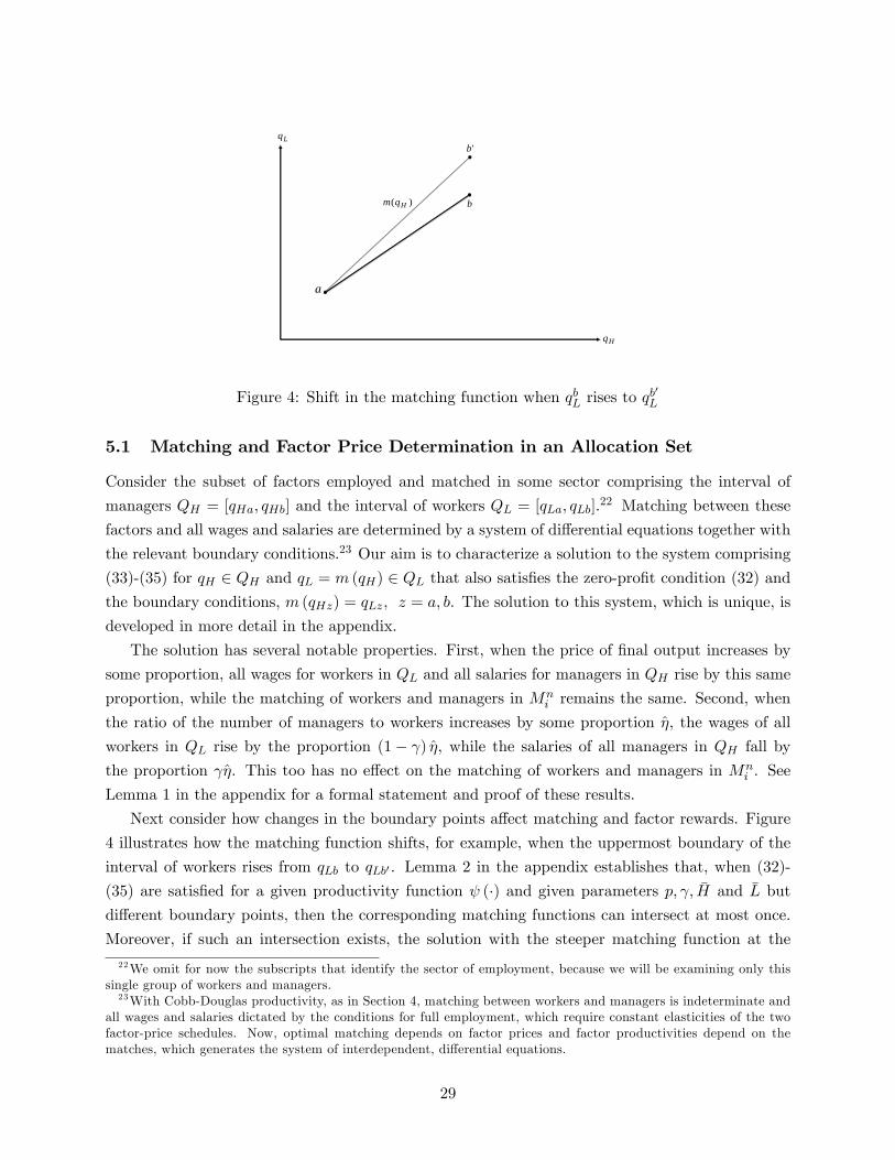
Lq
Hq
b
a
'b
)( Hqm
Figure 4: Shift in the matching function when qbL rises to qb′L
5.1 Matching and Factor Price Determination in an Allocation Set
Consider the subset of factors employed and matched in some sector comprising the interval of
managers QH = [qHa, qHb] and the interval of workers QL = [qLa, qLb].22 Matching between these
factors and all wages and salaries are determined by a system of differential equations together with
the relevant boundary conditions.23 Our aim is to characterize a solution to the system comprising
(33)-(35) for qH ∈ QH and qL = m (qH) ∈ QL that also satisfies the zero-profit condition (32) andthe boundary conditions, m (qHz) = qLz, z = a, b. The solution to this system, which is unique, is
developed in more detail in the appendix.
The solution has several notable properties. First, when the price of final output increases by
some proportion, all wages for workers in QL and all salaries for managers in QH rise by this same
proportion, while the matching of workers and managers in Mni remains the same. Second, when
the ratio of the number of managers to workers increases by some proportion η, the wages of all
workers in QL rise by the proportion (1− γ) η, while the salaries of all managers in QH fall by
the proportion γη. This too has no effect on the matching of workers and managers in Mni . See
Lemma 1 in the appendix for a formal statement and proof of these results.
Next consider how changes in the boundary points affect matching and factor rewards. Figure
4 illustrates how the matching function shifts, for example, when the uppermost boundary of the
interval of workers rises from qLb to qLb′ . Lemma 2 in the appendix establishes that, when (32)-
(35) are satisfied for a given productivity function ψ (·) and given parameters p, γ, H and L but
different boundary points, then the corresponding matching functions can intersect at most once.
Moreover, if such an intersection exists, the solution with the steeper matching function at the
22We omit for now the subscripts that identify the sector of employment, because we will be examining only thissingle group of workers and managers.23With Cobb-Douglas productivity, as in Section 4, matching between workers and managers is indeterminate and
all wages and salaries dictated by the conditions for full employment, which require constant elasticities of the twofactor-price schedules. Now, optimal matching depends on factor prices and factor productivities depend on thematches, which generates the system of interdependent, differential equations.
29
point of intersection also has lower wages and higher salaries for all ability levels that are common
to the two settings; see Lemma 6 in the appendix. In the figure, the matching functions that
apply before and after the increase in the upper boundary of worker ability necessarily intersect
at (qHa, qLa). By Lemma 2, we know that this can be the only intersection of the two curves, and
then the fact that a manager with ability qHb initially matches with a group of workers with ability
qLb but ultimately matches with a group of ability qLb′ implies that the matching function shifts
upward everywhere in the interior ofMni , as shown. Finally, Lemma 6 implies that wages fall for all
workers with qL ∈ [qLa, qLb] as a result of the addition of workers at the upper end of the interval.
The rematching depicted in Figure 4 has implications for within-industry wage and salary
inequality. Using (36) and (37) with qL0 = qLa and qH0 = qHa, we see that the wage schedule
rises with ability more slowly after the upper bound on worker ability increases to qLb′ . This is
so, because the original worker types are matched with less able managers after the expansion
in the interval of workers and, while the downgrades are detrimental to the productivity of all
workers, they are especially so for those with greater ability. Consequently, wage inequality among
workers with qL ∈ [qLa, qLb] narrows. Meanwhile, the managers all find better matches than before,
which raises their productivity, but especially so for the most able among them. Therefore, salary
inequality grows.
Similar reasoning can be used to find the shift in the matching function– and the wage and
salary responses– for changes in the other boundary points. For example, if the lower boundary of
the interval of managers rises from qHa to qHa′ , the matching function shifts downward (thereby
connecting a point to the right of a in Figure 4 with point b), and thus the manager types that remain
in the sector find themselves teamed with less able workers while all workers in QL find improved
matches with managers. Such rematching narrows the salary distribution while exacerbating wage
inequality. The key intuition is that, when the matches improve for some set of types of a factor,
the marginal products rise proportionally more for those types that are more able, in view of the
complementarities that are present.
We are ready to turn our attention to the sources of comparative advantage and the impact of
trade on wages and salaries.
5.2 Pattern of Trade
Consider the pattern of trade in an environment with sorting and matching. We note first that
two countries that share identical and homothetic preferences and similar distributions of factor
types but different relative factor endowments will not engage in trade unless the two industries
have different factor intensities. More formally, we state
Proposition 12 Suppose that Assumption 3 holds, φAH (qH) = φBH(qH) > 0 for all qH ∈ SAH =
SBH = SH , φAL (qL) = φBL (qL) > 0 for all qL ∈ SAL = SBL = SL, and γ1 = γ2 = γ. Then
XA1 /X
A2 = XB
1 /XB2 for all HA/LA and HB/LB.
30
We present the proof of this proposition here in the main text, because it helps to clarify the
economics of the result and what follows.
Proof. To prove the result, we examine the equilibrium response to an increase in the endowment
ratio H/L at given relative prices. The initial equilibrium is characterized by sets QLi and QHifor i = 1, 2, a matching function m (qH) that is strictly increasing in each of QH1 and QH2, and
wage and salary functions w (qL) and r (qH) that are continuous and strictly increasing in SL and
SH , respectively. These various functions satisfy (32)-(35) and an appropriate set of boundary
conditions. Now suppose that the endowment ratio H/L increases by some proportion η. Let
us conjecture that the sets QLi and QHi for i = 1, 2 and the matching function m (qH) remain
unchanged. Meanwhile, let the wage schedule rise by the proportion (1− γ) η and let the salary
schedule fall by the proportion γη, so that the factor-price ratio w [m (qH)] /r (qH) increases by the
proportion η for all qH ∈ SH . With these changes in factor prices, every firm increases its labor
demand (per manager) by the proportion η, irrespective of the ability of its managers. Thus, the
labor-market clearing condition (35) continues to be satisfied. Clearly, the new wage and salary
schedules are continuous and strictly increasing and they satisfy the first-order conditions, (33)
and (34), and the zero-profit condition (32). So, the new factor prices and the original matching
function and allocation sets indeed constitute an equilibrium after the increase in H/L. Output
grows in both sectors by the same proportion, γη, and thus relative outputs do not change.
When the industries differ in their factor intensities, the above construction– with equipropor-
tionate growth in both sectors, more workers per manager everywhere, and no change in matching–
does not work. Then a change in relative factor endowments does, in general, necessitate a change
in the composition of output. We focus on the case in which two countries that differ (only) in
relative factor endowments both display threshold equilibria; that is, in each country an interval
of the more able workers sorts to one sector while the remaining workers sort to the other, and
similarly for managers. We do not require that the more able workers sort to the same sector as the
more able managers, so we allow here for either an HH/LL equilibrium or an HL/LH equilibrium.
Let us begin with the latter. Suppose, for concreteness, that country A is relatively well endowed
with managers compared to country B (HA/LA > HB/LB) and that industry 1 is relatively
manager intensive compared to industry 2 (γ1 < γ2). Figure 5 depicts the qualitative features
of the inverse matching functions in such circumstances. In the figure, the solid curves depict
the matches that occur in country A when the more able workers with abilities qL ∈ [q∗L, qLmax]
sort to industry 1 and match there with the less able managers with abilities qH ∈ [qHmin, q∗H ].
As previously noted, the equilibrium features PAM within each sector but not across sectors. The
broken curves in the figure represent the matches that occur in country B. We show in the appendix
that the threshold q∗L always is smaller in the country that is relatively abundant in managers and
the threshold q∗H is larger in that country if and only if industry 1 is manager intensive; i.e., the
country with more managers per worker employs a greater fraction of its managers and a greater
fraction of its workers in the manager-intensive sector. As is apparent from the figure and Lemma
3 in the appendix (that allows at most one crossing within a sector), the inverse matching function
31

Hq
Lq
2sector
1sector
minLq maxLq*Lq
*Hq
minHq
maxHq
Figure 5: Sorting and matching: HL/LH equilibrium
Hq
Lq1sector
minLq maxLq*Lq
*Hq
minHq
maxHq
2sector
Figure 6: Sorting and matching: HH/LL equilibrium
for country B must lie below that for country A, both for the set of worker and manager types
that are employed in sector 1 in both countries and for the set of worker and manager types that
are employed in sector 2 in both countries. Among these types, the managers in country B achieve
better matches than their counterparts of similar ability in country A, whereas the workers in
country B achieve worse matches than their counterparts of similar ability in country A. Just the
opposite is true about the relative positions of the matching functions and the comparisons of the
matches when sector 2 is the more manager intensive. In either case, country A– with its relative
abundance of managers– always exports the manager-intensive good.
Now consider an HH/LL equilibrium in which the best workers and the best managers sort
to sector 1. The (inverse) matching function for such an equilibrium is continuous, monotonically
increasing, and has a slope that rises at the threshold q∗L, such as the one depicted for country A by
the solid curve in Figure 6. We show in the appendix that if HA/LA > HB/LB then the threshold
ability levels q∗L and q∗H both are greater in country A than in country B if and only if industry 2
32
Hq
Lq
2sector
1sector
minLq maxLq*Lq
*Hq
minHq
maxHq
a
d'
c' b'
a'
d
c b
*~Lq
*~Hq
Figure 7: Effects of a rise in p2 on matching: HL/LH equilibrium
is the labor-intensive sector. Again, the country that is relatively abundant in managers devotes
greater fractions of its managers and workers to production in the manager-intensive sector. It is
not clear whether managers of a given quality find better matches in country A or in country B,
or whether workers do so; the figure shows with broken curves the two possible outcomes when
HA/LA > HB/LB and γ1 > γ2. In any case, the manager-abundant country exports the manager-
intensive good.
We summarize in
Proposition 13 Suppose that: (i) Assumption 3 holds; (ii) countries A and B are identical except
for HA/LA > HB/LB; (iii) both countries are characterized by threshold equilibria with a single
cutoff for workers q∗L and for managers q∗H ; and (iv) γ1 6= γ2. Then country A exports the manager-
intensive good.
5.3 Effects of Trade on Income Distribution
The strong complementarities between factors that are implied by strict log supermodularity of
the productivity function induce PAM within sectors, as we have seen. The matches are fully
determined in the general equilibrium, unlike what occurs for Cobb-Douglas productivity, and so
changes in relative price generated by the opening of trade affect within-sector matching and the
within-sector income distribution. We turn now to the question of how trade affects these outcomes.
The opening of trade elevates the relative price of a country’s export good. For concreteness,
consider the country that exports good 2. In Figure 7, the solid curves cd and ab depict the (inverse)
matching function prior to the opening of trade for the case of an HL/LH equilibrium in which the
more able workers sort to industry 1. Now let p2 rise as a result of trade. This draws managers and
workers into sector 2, so that q∗H falls and q∗L rises.
24 The new boundary points are represented by
24Before any factor reallocation, the increase in p2 raises the value marginal product of the marginal workers and
33
w
Lq
2sector
1sector
minLq maxLq*Lq
e'
g'
h
g
f'h'
*~Lq
Figure 8: Effects of a rise in p2 on wages: HL/LH equilibrium
c′, d′, a′ and b′. As is evident from the figure, the new inverse matching function (represented by
the broken curves) lies below the old for all worker and manager types that remain in their original
industry of employment after the opening of trade. As a result, the opening of trade allows all
managers except those that switch sectors to achieve better matches than before, while causing all
workers except those that switch sectors to realize worse matches than before.
Proposition 14 summarizes these effects of trade on matching for the case of an HL/LH equi-
librium and reports the implications for wage and salary inequality.
Proposition 14 Suppose that: (i) Assumption 3 holds and (ii) the initial equilibrium is a thresholdequilibrium with an HL/LH sorting pattern. Then an increase in p2 (a) raises the labor cutoff q∗Land reduces the manager cutoff q∗H so that more workers and more managers are employed in sector
2; (b) worsens the matches for all workers except those that switch from sector 1 to sector 2; (c)
improves the matches for all managers except those that switch from sector 1 to sector 2; (d) reduces
within-industry wage inequality in both sectors and overall wage inequality in the economy; and (e)
increases within-industry salary inequality in both sectors and overall salary inequality.
In what follows, we discuss the effects of an increase in p2 on the wage distribution; the effects
on the salary distribution can be understood similarly.
Consider Figure 8, where the unlabeled thick curve represents the wage schedule in an initial
equilibrium. On impact– that is, prior to any resource reallocation– wages for workers with qL ∈[qLmin, q
∗L) rise in proportion to the increase in p2. These higher wages are depicted by the thin
curve gh in the figure. Were matching in each sector to remain the same despite the movement of
workers and managers from sector 1 to sector 2, we could trace the shadow wage schedule for sector
2 beyond gh and find the intersection with the wage schedule for sector 1 in order to identify the
managers in sector 2 relative to those in sector 1. As factors reallocate, marginal products change and rematchingoccurs. But we show in the appendix that these secondary effects cannot overturn the impact effects, so that q∗Hmust fall and q∗L must rises in the setting described by the figure.
34
new cutoff ability level. However, the matching functions in each sector do not remain the same in
the wake of a price change, as we have already seen.
Let us refer back to Figure 7 and suppose, counterfactually, that as the cutoff for managers
declines to its new equilibrium level at q∗H there is no change in the cutoff for workers. Were this to
be so, the new inverse matching function would comprise a curve connecting points c′ and d in sector
2, along with a curve connecting points a with b′ in sector 1. Such a shift would imply a flatter
relationship between wages and ability in each sector, considering the strict log supermodularity of
the productivity functions. Moreover, the new inverse matching function would be flatter at point a
than the old. By Lemma 6 in the appendix (as discussed in Section 5.1), the wage of a worker with
ability q∗L employed in sector 1 would fall. We indicate this drop in wage by the point e′ in Figure
8 and draw the curve e′f ′ to represent the slower rise of wages as a function of ability. Meanwhile,
in sector 2, the inverse matching function is steeper at point d of Figure 7, where workers of ability
q∗L match with managers of ability qHmax. So the wage of a worker with ability q∗L employed in
sector 2 would be at a point such as h′ in Figure 8, higher than before. Since wages rise at a slower
pace in this sector too, the hypothetical wage curve for sector 2 must be above gh, such as at g′h′
in the figure.
We see that our counterfactual assumption of no change in the cutoff for workers cannot be
sustained. The gap in wages between points e′ and h′ induces movement of workers from sector 1
to sector 2. This generates an additional rotation of the two segments of the matching function in
Figure 7 to curves between points a′ and b′ for sector 1 and between points c′ and d′ in sector 2.
Compared to the matching that would occur without a change in q∗L, there is a further worsening
of matches for workers, so that wages rise even more slowly than along e′f ′ and g′h′ in Figure 8.
The movement of workers from sector 1 to sector 2 makes the inverse matching function steeper in
sector 2 and flatter in sector 1 for the manager with ability q∗H . The former implies a decline in the
wage of the worker with ability qLmin to a point below g′ and a flattening of the wage schedule for
workers in sector 1. The latter implies a rise in the wage of the worker with ability qLmax and a
steepening of the wage schedule relative to e′f ′. Together, these shifts eliminate the gap in wages
for the (new) marginal worker with ability q∗L.
Evidently, wage inequality falls among workers originally in industry 2 and among those remain-
ing in industry 1. Take for example any two workers q′L and q′′L such that qLmin ≤ q′L < q′′L ≤ q∗L.
Both workers see their match deteriorate as a result of the increase in the price of good 2, but
the rematching harms the worker with ability q′′L by relatively more due to the presence of strong
complementarities between factor types. The same is true for any pair of workers with abilities
between q∗L and qLmax. Finally, consider a pair of workers that switch sectors; i.e., those that
have ability levels between q∗L and q∗L. The relative wage of the less able worker in this pair must
rise, because the elasticity of the wage schedule in (33) is determined after the price change by the
elasticity of the productivity function in sector 2, whereas before it was determined by the elasticity
of the productivity function in sector 1. Since the more able workers sort to sector 1, it must be
that the former elasticity is smaller than the latter. It follows that wage inequality declines also
35
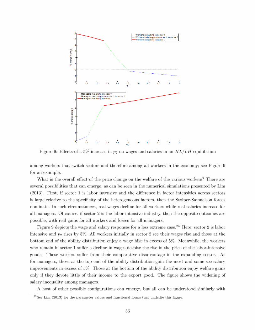
Figure 9: Effects of a 5% increase in p2 on wages and salaries in an HL/LH equilibrium
among workers that switch sectors and therefore among all workers in the economy; see Figure 9
for an example.
What is the overall effect of the price change on the welfare of the various workers? There are
several possibilities that can emerge, as can be seen in the numerical simulations presented by Lim
(2013). First, if sector 1 is labor intensive and the difference in factor intensities across sectors
is large relative to the specificity of the heterogeneous factors, then the Stolper-Samuelson forces
dominate. In such circumstances, real wages decline for all workers while real salaries increase for
all managers. Of course, if sector 2 is the labor-intensive industry, then the opposite outcomes are
possible, with real gains for all workers and losses for all managers.
Figure 9 depicts the wage and salary responses for a less extreme case.25 Here, sector 2 is labor
intensive and p2 rises by 5%. All workers initially in sector 2 see their wages rise and those at the
bottom end of the ability distribution enjoy a wage hike in excess of 5%. Meanwhile, the workers
who remain in sector 1 suffer a decline in wages despite the rise in the price of the labor-intensive
goods. These workers suffer from their comparative disadvantage in the expanding sector. As
for managers, those at the top end of the ability distribution gain the most and some see salary
improvements in excess of 5%. Those at the bottom of the ability distribution enjoy welfare gains
only if they devote little of their income to the export good. The figure shows the widening of
salary inequality among managers.
A host of other possible configurations can emerge, but all can be understood similarly with
25See Lim (2013) for the parameter values and functional forms that underlie this figure.
36
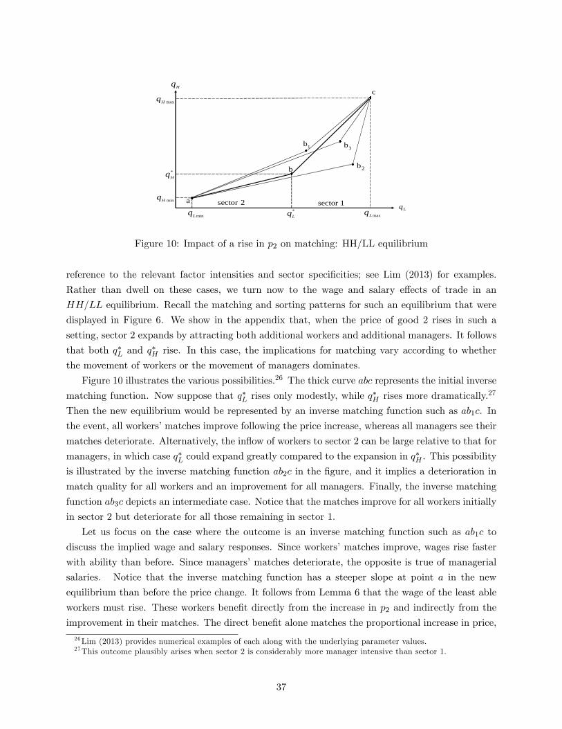
Hq
Lq1sector
minLq maxLq*Lq
*Hq
minHq
maxHq
2sectora
c
1b
b
3b
2b
Figure 10: Impact of a rise in p2 on matching: HH/LL equilibrium
reference to the relevant factor intensities and sector specificities; see Lim (2013) for examples.
Rather than dwell on these cases, we turn now to the wage and salary effects of trade in an
HH/LL equilibrium. Recall the matching and sorting patterns for such an equilibrium that were
displayed in Figure 6. We show in the appendix that, when the price of good 2 rises in such a
setting, sector 2 expands by attracting both additional workers and additional managers. It follows
that both q∗L and q∗H rise. In this case, the implications for matching vary according to whether
the movement of workers or the movement of managers dominates.
Figure 10 illustrates the various possibilities.26 The thick curve abc represents the initial inverse
matching function. Now suppose that q∗L rises only modestly, while q∗H rises more dramatically.27
Then the new equilibrium would be represented by an inverse matching function such as ab1c. In
the event, all workers’matches improve following the price increase, whereas all managers see their
matches deteriorate. Alternatively, the inflow of workers to sector 2 can be large relative to that for
managers, in which case q∗L could expand greatly compared to the expansion in q∗H . This possibility
is illustrated by the inverse matching function ab2c in the figure, and it implies a deterioration in
match quality for all workers and an improvement for all managers. Finally, the inverse matching
function ab3c depicts an intermediate case. Notice that the matches improve for all workers initially
in sector 2 but deteriorate for all those remaining in sector 1.
Let us focus on the case where the outcome is an inverse matching function such as ab1c to
discuss the implied wage and salary responses. Since workers’matches improve, wages rise faster
with ability than before. Since managers’matches deteriorate, the opposite is true of managerial
salaries. Notice that the inverse matching function has a steeper slope at point a in the new
equilibrium than before the price change. It follows from Lemma 6 that the wage of the least able
workers must rise. These workers benefit directly from the increase in p2 and indirectly from the
improvement in their matches. The direct benefit alone matches the proportional increase in price,
26Lim (2013) provides numerical examples of each along with the underlying parameter values.27This outcome plausibly arises when sector 2 is considerably more manager intensive than sector 1.
37
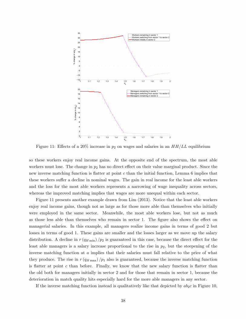
Figure 11: Effects of a 20% increase in p2 on wages and salaries in an HH/LL equilibrium
so these workers enjoy real income gains. At the opposite end of the spectrum, the most able
workers must lose. The change in p2 has no direct effect on their value marginal product. Since the
new inverse matching function is flatter at point c than the initial function, Lemma 6 implies that
these workers suffer a decline in nominal wages. The gain in real income for the least able workers
and the loss for the most able workers represents a narrowing of wage inequality across sectors,
whereas the improved matching implies that wages are more unequal within each sector.
Figure 11 presents another example drawn from Lim (2013). Notice that the least able workers
enjoy real income gains, though not as large as for those more able than themselves who initially
were employed in the same sector. Meanwhile, the most able workers lose, but not as much
as those less able than themselves who remain in sector 1. The figure also shows the effect on
managerial salaries. In this example, all managers realize income gains in terms of good 2 but
losses in terms of good 1. These gains are smaller and the losses larger as we move up the salary
distribution. A decline in r (qHmin) /p2 is guaranteed in this case, because the direct effect for the
least able managers is a salary increase proportional to the rise in p2, but the steepening of the
inverse matching function at a implies that their salaries must fall relative to the price of what
they produce. The rise in r (qHmax) /p1 also is guaranteed, because the inverse matching function
is flatter at point c than before. Finally, we know that the new salary function is flatter than
the old both for managers initially in sector 2 and for those that remain in sector 1, because the
deterioration in match quality hits especially hard for the more able managers in any sector.
If the inverse matching function instead is qualitatively like that depicted by ab2c in Figure 10,
38

then the outcomes are just the opposite. Low-ability managers gain from an increase in p2, because
their value marginal product rises in proportion to the price hike and rises further as a result of
the rematching. High-ability managers lose in real terms, because r (qHmax) /p1 falls. All wages
rise, albeit less than in proportion to the price increase. The wage hikes are proportionally greatest
for those at the bottom end of the ability distribution. As a result of these factor price responses,
wage inequality declines both within and between sectors, whereas salaries become more unequal
within sectors, but those at the bottom who are employed in sector 2 gain relative to those at the
top who are employed in sector 1.
Finally, if the inverse matching function is like that depicted by ab3c, then the outcomes are a
mix of those described above. In this case, all workers initially employed in sector 2 must benefit
from the price increase, while all managers initially employed in sector 1 must lose. The low-ability
managers and the high-ability workers both gain in compensation relative to the price of good 1,
but lose relative to the price of good 2. Lim (2013) provides numerical examples.
Clearly, by allowing for worker and manager heterogeneity and strong complementarities be-
tween these factors, we can accommodate a rich set of possible effects of globalization on the wage
and salary distributions. Some forces are familiar. For example, trade tends to benefit the factor
(managers or workers) used intensively in the export industry. And trade tends to benefit those
types of each factor that have a comparative advantage in the export sector. But other forces are
new. Trade can improve the matches for some factor in one sector or in both. If it does so, the
productivity of the factor will rise beyond what is predicted by the usual forces, and especially so
for the more able types. Predictions about which types will gain or lose– and about whether the
income distribution will widen or narrow in response to an opening of trade– may require detailed
information about technologies, factor intensities, and distributions of talent and know-how.
5.4 Effects of Trade on Measured Productivity
We conclude this section with a brief discussion of the effects of trade on measured productivity.
We shall see that the subtle implications of rematching introduce ambiguities here, just as they do
for the links between trade and factor prices.
As before, we measure productivity using factor quantities and the Cobb-Douglas nature of the
production technology. In particular, we write
Xi = AiLγii H
1−γii ,
where Li and Hi are aggregate employment of workers and managers, respectively, in sector i, and
Ai captures TFP. The firms in sector i devote a fraction γi of their revenues to wages and the
remaining fraction to salaries. It follows that γipiXi =∫q∈QLi w (q)φL (q) dq and (1− γi) piXi =∫
q∈QHi r (q)φH (q) dq. Using these expressions together with the expressions for aggregate employ-
39
ment of workers and managers in each sector, we can write
Ai = γ−γii (1− γi)−(1−γi)
(E[w (qL)
pi
∣∣∣∣ qL ∈ QLi])γi (E [ r (qH)
pi
∣∣∣∣ qH ∈ QHi])1−γi .Evidently, measured productivity in a sector varies with the average own-product real wage paid
to the workers employed there and the average own-product real salary paid to managers. These
averages reflect, of course, the average marginal products of the various factor types.
Consider, for example, a country that has an HH/LL sorting pattern, such as that depicted
in Figure 6. We know that an increase in p2 draws more of both factors into sector 2. The
workers and managers that change sector raise the average marginal products everywhere, because
these marginal workers and managers have higher abilities than those initially employed in sector
2 and lower abilities than those that remain employed in sector 1. If matching were to remain as
before, then measured TFP would rise in both sectors. This is much the same as for the case of
Cobb-Douglas productivity, which we considered previously in Section 4.28
But, as we know, the matches do not remain the same, and the rematching impacts the marginal
productivity of every manager and worker. Consider further the example of factor-price responses
that is depicted in Figure 11. In sector 2, own-product real wages rise and own-product real salaries
decline. This reflects an improvement in match quality for the workers initially employed in sector
2 and a deterioration in match quality for the managers there. The former raises measured TFP
and the latter lowers it, with the net effect depending in a complex way on factor intensities and
the densities of the factor distributions. Meanwhile, the own-product real wages fall in sector 1 and
the own-product real salaries rise there, as a result of the rematching that occurs. Again, the net
effects are ambiguous. More generally, the rematching of factors in a sector raises the productivity
of one factor while reducing it for the other. The effects of trade on measured TFP are thus bound
to be an empirical matter.
6 Labor Market Frictions
Until now, we have assumed that labor markets flawlessly and costlessly allocate the various types of
labor to their most effi cient uses. Of course, the smooth functioning of labor markets is notoriously
suspect and worker heterogeneity would only seem to exacerbate the potential diffi culties. In this
section, we show how a simple form of search frictions can be incorporated into the analysis. The
extension allows us to discuss the distribution of unemployment rates across the ability spectrum
alongside the distribution of wages.
To keep matters simple, we continue to assume a frictionless market for managers. In other
words, firms can hire managers of whatever ability and in whatever numbers they wish by offering
28Note, however, that if a country has an HL/LH sorting pattern, the expansion of sector 2 leads to an improvementin average worker ability but a decline in average manager ability in both sectors. Then, even without consideringthe effects of rematching, the implications for measured TFP are ambiguous.
40

a competitive salary.29 But firms must search for their workers and workers for jobs. We follow
Peters (1991, 2000), Acemoglu and Shimer (1999), Burdett et al. (2001), Eeckhout and Kircher
(2010a), and others in modeling labor-market frictions with “directed search,”whereby firms post
costly “vacancies” and workers and firms meet randomly. We extend this approach to allow for
worker heterogeneity and multiple hires per firm.
Suppose, as before, that the output in industry i of a production unit comprising a manager of
ability qH and ` workers of ability qL is given by (1). A firm (or entrepreneurial manager) hires
workers by posting vacancies. Each posting costs ci units of the the firm’s final output. A posting
lists the ability level qL that the firm targets and the wage ω that it will pay to any employee of
this type. We assume that the firm can commit to these job attributes, in the sense that it will not
hire workers with ability different from the posted level nor attempt to renegotiate its wage offer
after it meets with a job applicant.30 The firm chooses v, the number of its vacancies, to maximize
profits.
Workers are risk neutral. Each worker applies for a single job of his choosing.31 Workers
consider only the jobs for which they are qualified, because firms will not hire types different from
those targeted in their announcements. Among relevant jobs, each worker applies for the position
that offers the greatest expected income. In equilibrium, workers must be indifferent among the
range of openings posted for their type.
Let s be the number of workers seeking jobs at a firm that has posted v vacancies. We assume
that the search process results in the consummation of M (s, v) jobs, where
M(s, v) = Bsτv1−τ , (38)
B > 0 and 0 < τ < 1.32 For a firm, the probability of filling any given vacancy is δv (s/v) =
B (s/v)τ , whereas for a worker the probability of a successful application is δs (s/v) = B (s/v)−(1−τ).
The former is increasing in s/v, while the latter is decreasing in s/v; i.e., a firm’s chances of filling
a vacancy improve and a worker’s chances of landing a job decline with the number of applicants
per posting.
29Perhaps the best way to justify this assumption is to imagine the manager as an entrepreneur, as in Lucas (1978).Then it is the manager that searches for employees and her salary amounts to the residual profits after wages andhiring costs are paid. Alternatively, one might think of the second factor as being capital, instead of managers, inwhich case an assumption that firms can readily find machines of the quality they desire is not so hard to swallow.30Alternatively, we could allow a firm to post a wage schedule and to hire any worker it happens to meet at the
wage specified by the schedule. If each vacancy generates at most one meeting with a job applicant, then it is neveroptimal for the firm to induce applications from more than one type of worker; see Eeckhout and Kircher (2010a,2010b) for proof of this assertion in related environments. In such circumstances, there is no loss of generality inassuming that the firm targets only one type of worker. Shimer (2005) studies a setting in which one vacancy canresult in multiple meetings with potential employees. Then, in the general, it is optimal for any firm to induceapplications from several different types. We do not explore this possibility here.31This assumption is common in the literature on direct search. Galenianos and Kircher (2009) describe settings
in which the restriction to one application per worker does not change the qualitative predictions of the model.32The job-search literature refers to M (s, v) as a “matching function” but we eschew that terminology so as to
avoid confusion with the function that “matches”workers and managers, qL = m (qH). The Cobb-Douglas form forM (·) is common in the literature, and is implicitly coupled with the usual restriction that B is suffi ciently small toimply meeting probabilities below unity for both vacancies and workers.
41

Now let w(qL) be the expected wage that workers of type qL obtain in equilibrium, which each
firm takes as given. A firm must offer at least this expected wage or it will find itself without
applicants; and it has no reason to offer more. In equilibrium, a firm with v vacancies that offers
a wage ω targeted to workers with ability qL attracts s applicants, where s is such as to make
the applicants indifferent between the firm’s openings and their other opportunities; i.e., s solves
δs(s/v)ω = w(qL). Using (38), this can be rewritten as
s
v=
[Bω
w(qL)
] 11−τ
. (39)
Equation (39) is the main building block in a model with directed search; it ties the wage an-
nouncement ω to the endogenous number of applications per vacancy s/v, which in turn determines
the firm’s fill rate, δv(s/v).33 Given the expected wage w(qL), the firm can use (39) to compute
the number of workers that will seek its employment and thus the number of workers ` = M (s, v)
that it will succeed in hiring. Again using (38), together with (39), we see that a firm that posts v
vacancies targeted at workers with ability qL and that offers a wage of ω manages to hire ` workers,
where
` = B1
1−τ
[ω
w(qL)
] τ1−τ
v. (40)
Evidently, hires are proportional to the number of vacancies and rise with the ratio of the firm’s
wage offer to the workers’outside option.
Now consider the profit-maximization problem facing a firm with a manager of ability qH that
chooses to operate in industry i. The firm pays piciv to post v vacancies and pays ω to each of the
` workers that it eventually hires. Its profits are given by
πi = piψi(qH , qL)`γi − ω`− piciv − r (qH) ,
where r (qH) as before represents the manager’s salary. Then, using (39), (23), and the first-order
condition for the firm’s optimal choice of wage offer, we can re-express its profits as
πi = piϕi(qH , qL)sζi − w(qL)s− r (qH) ,
where
ϕi(qH , qL) ≡ [1− (1− τ) γi]
[(1− τ) γi
ci
] (1−τ)γi1−(1−τ)γi
Bγi
1−(1−τ)γi ψi(qH , qL)1
1−(1−τ)γi
33Peters (1991, 2000) and Burdett et al. (2001) provide microfoundations for a relationship similar to (39). Theybegin by assuming a finite number of jobs and vacancies and then allow the economy to grow large without bound.This generates a balls—and-urns type function for applicants per vacancy, rather than the Cobb-Douglas form that ismore commonly assumed. Galenianos and Kircher (2012) extends their setup to generate CES and Cobb-Douglasmatching functions. With but a few exceptions, the literature on directed search specifies the matching functionindividually for each vacancy, and we follow in this tradition.
42
and
0 < ζi ≡τγi
1− (1− τ) γi< 1.
Notice that this expression for profits has the same mathematical properties as the profit func-
tion πi = piψi(qH , qL)`γi −w(qL)`− r (qH) that we encountered in Section 5, because if ψi(qH , qL)
satisfies part (ii) of Assumption 3 (i.e., it is strictly increasing, continuously differentiable, and
strictly log supermodular) so too does ϕi(qH , qL), and ζi like γi is between zero and one.34 In other
words, the firm’s choice about the number of job applications to invite in a setting with search
frictions is much like its choice about the number of workers to hire in a setting without them. The
first-order condition for s implies
s =
[δipiϕi (qH , qL)
w(qL)
] 11−δi
, (41)
which generates the profit function
πi (qH , qL) = ζip1
1−δii ϕi (qH , qL)
11−ζi w (qL)
− ζi1−ζi − r (qH) ,
where ζi ≡ ζζi
1−ζii (1− ζi). This expression has much the same form as (30), which applies in the
absence of search frictions. Finally, the analog to the labor-market clearing condition from before is
the requirement that the aggregate number of applications induced by firms operating in industry
i and targeting workers of ability qL must equal the number of workers with that ability level that
sort to the sector in search of a job. With these observations, we conclude that the equilibrium
expected wage function w (qL), salary function r (qH) and matching function qL = m (qH) can be
characterized as the solution to three differential equations analogous to (33)-(35), a zero profit
condition analogous to (32), and a set of boundary conditions. Evidently, comparative advantage
again derives from a country’s relative factor endowments and its distributions of worker and
manager ability. Moreover, since ζ1 > ζ2 if and only if γ1 > γ2, the cross-sectoral differences in
factor intensities interact with differences in factor endowments to determine the pattern of trade
in much the same way as before. The search frictions themselves are not an independent source of
comparative advantage so long as these frictions are similar in the two sectors.35
The model with search frictions features different employment rates across the range of ability
levels. In order to discuss the impact of trade on employment, we combine the optimal choice of
wage offer with a firm’s desired number of applications per manager to derive
ω (qL) = B−γi(
1− ττpici
)−(1−τ)γiw(qL)1−(1−τ)γi .
34Note too that if ψi(qH , qL) is a product of power functions, as in Section 4, so too is ϕi(qH , qL). And if ψi(qH , qL)has a constant elasticity of substitution between qH and qL, so too does ϕi(qH , qL).35 If the number of meetings in (38) varies by sector, then it is immediate from the definition ζi ≡ τ iγi/(1 −
(1− τ i) γi) that the search process constitutes an additional source of comparative advantage.
43
The expected wage w (qL) must be an increasing function of ability. It follows that, among
workers that seek employment in a given industry i, those with greater ability see higher posted
wages for the jobs they pursue. Next, we substitute this expression for ω (qL) into (40) to derive
an expression for the employment rate for workers of ability qL, namely
`
s= B
γi
(1− ττci
)(1−τ)γi [w(qL)
pi
](1−τ)γi. (42)
Since the expected wage on the right-hand side is an increasing function of ability, we conclude
that so too is the employment rate among workers seeking jobs in a given industry. We record our
findings in
Proposition 15 Suppose that Assumption 3 holds. Let q′L, q′′L ∈ Qi, with q′L > q′′L. Then the job
listings targeted to workers with ability q′L offer a higher expected wage and a greater probability of
employment than those targeted to q′′L. The opening of trade causes within-sector wage inequality
and employment inequality to move in the same direction.
In a setting with search frictions, the opening of trade affects differently the employment rates
at different ability levels. Let us consider just one example to illustrate how the analysis can be
performed. Suppose a country has an HL/LH sorting pattern such as that depicted in Figure 5
and that the country exports good 2. The opening of trade generates an increase in p2. Figure
7 shows the effects of such a price change on the matching of worker and manager types in each
sector. As we have seen, the workers who do not switch sectors find themselves teamed with a less
able manager than before. Now, Figure 9 can be interpreted as illustrating the predicted impact
on expected wages. The figure shows an increase in w (qL) /p2 for some of the least able workers,
who sort to sector 2, a decline in w (qL) /p2 for some moderately able workers that sort to sector
2, and a decline in w (qL) /p1 for the most able workers, who sort to sector 1.
We refer now to equation (42), which applies in the presence of search frictions. The equation
implies that the employment rate rises for the aforementioned group of least able workers while
it falls for those with moderate and high ability. Overall, the distribution of employment rates
becomes more equal across the worker population. Of course, the effects of trade on the distribution
of employment would be just the opposite if the country instead imported good 2. Evidently, trade
can widen or narrow the inequality in employment rates across the ability distribution according to
the sorting pattern that is realized and the comparative advantage of the country. The determinants
of these outcomes in an economy with directed search are similar to the determinants of wage
inequality in an economy that has frictionless labor markets.
7 Concluding Remarks
In this paper, we have extended the familiar two-sector, two-factor model of international trade
to include heterogeneous factors of production. In a model with factor heterogeneity, we can
44

examine the determinants of factor sorting to industries and the determinants of factor matching
within industries. When the productivity of a production unit depends on both the manager’s and
workers’abilities– and particularly when there are strong complementarities between the two– the
forces that guide sorting and matching become inextricably linked. The economy-wide pattern of
factor assignments can be subtle and complex even in the presence of strong complementarities
that dictate positive assortative matching within every sector.
A model with heterogeneous factors allows a more complete analysis of the distributional effects
of trade than is possible in one with homogeneous factors. In particular, we can ask how the opening
of trade or trade liberalization affects the wage and salary distributions over the entire range of
compensation levels. In general, there are three considerations that determine the effects of trade
on the income of a particular individual. First, as in the standard Heckscher-Ohlin world with
homogeneous factors, there is the question of whether the export sector is intensive in the use of
workers or managers. Second, as in the standard Ricardo-Viner world with factor specificity, there
is the question of whether an individual’s type generates a personal comparative advantage in the
export sector or the import-competing sector. Finally, and most novel, there is the question of how
trade affects the individual’s match with other factors of production. If a change in trade conditions
causes a worker to rematch with a better manager than before, then his productivity will improve
and his wage will receive an upward boost. If instead a worker’s match deteriorates, then his wage
may suffer. Interestingly, the effects of trade on wage or salary inequality across sectors may run
counter to the effects on inequality within a sector.
We have shown that the Heckscher-Ohlin theorem extends to a setting with heterogeneous
factors provided that the countries share similar distributions of worker and managerial talent.
But we have also noted how differences in the distributions of talent can be an independent source
of comparative advantage. A country that has more able workers than another– in the sense of
a rightward shift in the talent distribution– will produce relatively more of the good for which
productivity responds more elastically to ability. We have also seen how trade affects measured
TFP in settings where individuals’talents are not fully observable to the analyst. The equilibrium
sorting pattern dictates whether the marginal factors that enter or exit an industry as the result of
trade are more or less productive than the average.
Finally, we have incorporated search frictions. In a simple setting with directed search, firms
create vacancies and make wage offers to workers of a targeted type. In such a setting, trade affects
not only the distribution of wages but also the distribution of employment rates across the different
types of workers. We provide an example in which the main insights from the earlier analysis
carry over without modification to an environment with unemployment. But much work remains
to the elucidate the connection between trade and the effi ciency of matching and to understand
how globalization affects equilibrium unemployment rates for different types of workers.
45
References
[1] Acemoglu, Daron and Shimer, Robert, 1999. “Holdups and Effi ciency With Search Frictions,”
International Economic Review 40 (4), 827—849. ”
[2] Antràs, Pol, Garicano, Luis and Rossi-Hansberg, Esteban, 2006. “Offshoring in a Knowledge
Economy,”Quarterly Journal of Economics 121(1), 31-77.
[3] Bombardini, Matilde, Gallipoli, Giovanni and Pupato, Germán, 2012. “Skill Dispersion and
Trade Flows,”American Economic Review 102(5), 2327-48.
[4] Burdett, Kenneth, Shi, Shouyong. and Wright, Randall, 2001.“Pricing and Matching With
Frictions,”Journal of Political Economy 109 (5), 1060—1085.
[5] Costinot, Arnaud, 2009. “An Elementary Theory of Comparative Advantage,”Econometrica
77(4), 1165-92.
[6] Costinot, Arnaud and Vogel, Jonathan, 2010. “Matching and Inequality in the World Econ-
omy,”Journal of Political Economy 118(4), 747-86.
[7] De Loecker, Jan, 2011. “Product Differentiation, Multiproduct Firms and Estimating the
Impact of Trade Liberalization on Productivity,”Econometrica 79 (5), 1407-51.
[8] Eeckhout, Jan and Kircher, Philipp, 2010a. “Sorting and Decentralized Price Competition,”
Econometrica 78 (2), 439-74.
[9] Eeckhout, Jan and Kircher, Philipp, 2010b. “Sorting vs Screening - Search Frictions and Com-
peting Mechanisms,”Journal of Economic Theory 145 (4), 1354-85.
[10] Eeckhout, Jan and Kircher, Philipp, 2012. “Assortative Matching with Large
Firms: Span of Control over More versus Better Workers.” Downloadable at
http://personal.lse.ac.uk/kircher/Papers/sorting-and-factor-intensity.pdf
[11] Galenianos, Manolis and Kircher, Philipp, 2009.“Directed Search with Multiple Job Applica-
tions,”Journal of Economic Theory 114 (2), 445-71.
[12] Galenianos, Manolis and Kircher, Philipp, 2012. “On the Game-theoretic Foundations of Com-
petitive Search Equilibrium,”International Economic Review 53 (1), 1-21.
[13] Garicano, Luis, 2000. “Hierarchies and the Organization of Knowledge in Production,”Journal
of Political Economy 108(5), 874-904.
[14] Grossman, Gene M., 1983. “Partially-Mobile Capital: A General Approach to Two-Sector
Trade Theory,”Journal of International Economics 15(1-2), 1-17.
[15] Grossman, Gene M. and Maggi, Giovanni, 2000. “Diversity and Trade,”American Economic
Review 90(5), 1255-75.
46
[16] Helpman, Elhanan, Itskhoki, Oleg, Muendler, Marc-Andreas and Redding, Stephen, 2012.
“Trade and Inequality: From Theory to Estimation,”NBER Working Paper No. 17991.
[17] Jones, Ronald, 1971. “A Three-Factor Model in Theory, Trade and History,”J. Bhagwati, R.
Jones, R. Mundell and J. Vanek, eds., Trade, Balance of Payments and Growth, Amsterdam:
North-Holland.
[18] Lim, Kevin, 2013. “Numerical Simulations for ‘Matching and Sorting in the Global Economy’.”
Downloadable at http://www.princeton.edu/~grossman/grossman_working_papers.htm.
[19] Lucas, Robert E., Jr., 1978. “On the Size Distribution of Business Firms,”The Bell Journal
of Economics 9 (2), 508-23.
[20] Mussa, Michael, 1982. “Imperfect Factor Mobility and the Distribution of Income,” Journal
of International Economics 12(1-2), 125-141.
[21] Ohnsorge, Franziska and Trefler, Daniel, 2007. “Sorting it Out: International Trade with
Heterogeneous Workers,”Journal of Political Economy 115(5), 868-92.
[22] Pavcnik, Nina, 2002. “Trade Liberalization, Exit, and Productivity Improvement: Evidence
from Chilean Plants,”Review of Economic Studies 69 (1), 245-76.
[23] Peters, Michael, 1991. “Ex ante Price Offers in Matching Games: Non Steady States,”Econo-
metrica 59 (5), 1425—54.
[24] Peters, Michael, 2000. “Limits of Exact Equilibria for Capacity Constrained Sellers With
Costly Search,”Journal of Economic Theory 95 (2), 139—68.
[25] Roy, Andrew D., 1951. “Some Thoughts on the Distribution of Earnings,”Oxford Economic
Papers 3(2), 135-46.
[26] Ruffi n, Roy, 1988. “The Missing Link: The Ricardian Approach to the Factor Endowment
Theory of International Trade,”American Economic Review 78(4), 759-72.
[27] Sampson, Thomas, 2012. “Selection into Trade and Wage Inequality,”CEP Discussion Papers
No. 1152, Centre for Economic Policy Performance.
[28] Sattinger, Michael, 1975. “Comparative Advantage and the Distributions of Earnings and
Abilities,”Econometrica 43 (3), 455-68.
[29] Shimer, Robert, 2005. “The Assignment of Workers to jobs in an Economy with Coordination
Frictions,”Journal of Political Economy 113(5), 996-1025.
[30] Trefler, Daniel, 2004. “The Long and Short of the Canada-U. S. Free Trade Agreement,”
American Economic Review 94 (4), 870-95.
[31] Yeaple, Stephen R, 2005. “A Simple Model of Firm Heterogeneity, International Trade, and
Wages,”Journal of International Economics 65(1), 1-20.
47

Appendix
This appendix provides proofs of results stated in the main text.
Proofs for Section 3
First, note that in the system comprising (6)-(9), a proportional increase in the number of managers and
workers, H and L, raises H1 by the same factor of proportionality and leaves q∗L and the wage anchors w1
and w2 unchanged. Therefore, in this case, the output of each good rises proportionately, so that the ratio
X1/X2 does not change. It follows that in order to find the impact of H/L on X1/X2, it suffi ces to find the
impact of L on the relative supply.
Differentiating the equilibrium system (6)-(9), we obtain1 −1 sL (q∗L) 0
− γ11−γ1
γ21−γ2
0 0
0 E21−γ2
Lψ2 (q∗L)1/γ2 φL (q∗L) q∗L E2H1/H2
E11−γ1
0 −Lψ1 (q∗L)1/γ1 φL (q∗L) q∗L −E1
w1
w2
q∗LH1
(43)
=
0
0
−E2−E1
L+
0
− 11−γ10E11−γ1
p1,
where
Ei = Hi
(γipiwi
) 11−γi
, i = 1, 2; H2 = H −H1.
Here Ei represents the aggregate measure of effective labor units (defined as above) allocated to sector i.
Let Dho be the determinant of the matrix on the left-hand side of (43). Then
Dho = LφL (q∗L) q∗Lw (q∗L)
w1w2H1
(γ2 − γ1)2
(1− γ1)2
(1− γ2)2 +
sL (q∗L)
(1− γ1) (1− γ2)
(γ1 + γ2
H1
H2
)E1E2,
because (8), (9) and the definition of Ei imply that
ψ1 (q∗L)1/γ1 E2
H1
H2− ψ2 (q∗L)
1/γ2 E1 = H1
[ψ1 (q∗L)
1/γ1
(γ2p2w2
) 11−γ2
− ψ2 (q∗L)1/γ2
(γ1p1w1
) 11−γ1
](44)
=w (q∗L)
w1w2H1
γ2 − γ1(1− γ1) (1− γ2)
. (45)
It follows that sL (q∗L) > 0⇒ Dho > 0.
We now use (43) to calculate the response of H1 to an increase in labor supply L, which yields
H1Dho =γ1 − γ2
(1− γ1) (1− γ2)
[E1Lψ2 (q∗L)
1/γ2 φL (q∗L) q∗L + E2Lψ1 (q∗L)1/γ1 φL (q∗L) q∗L + E1E2sL (q∗L)
] L.Therefore, given sL (q∗L) > 0, an increase in labor supply raises the number of managers in sector 1 if and
only if sector 1 is labor intensive, i.e., γ1 > γ2; otherwise it raises the number of managers in sector 2. When
H1 increases, the relative supply X1/X2 increases as well. It follows that the country with relatively more
48

workers produces relatively more of the labor-intensive good and exports that good. This proves Proposition
2.
Next we calculate the response of the two wage anchors to changes in the price of good 1. From (43)
and (44), we obtain
w1Dho = LφL (q∗L) q∗L1
1− γ1w (q∗L)
w1w2H1
γ1 − γ2(1− γ1) (1− γ2)
p1 + sL (q∗L)E1E2
(1− γ1) (1− γ2)
(1 + γ2
H1
H2
)p1,
w2Dho = LφL (q∗L) q∗L1
1− γ1w (q∗L)
w1w2H1
γ1 − γ2(1− γ1) (1− γ2)
p1 − sL (q∗L)E1E21− γ1
H1
H2p1.
It follows that (w1 − w2) /p1 > 0 when sL (q∗L) > 0, which implies that w1 > w2 when p1 > 0, as argued in
part (i) of Proposition 4. We also calculate the response of the salary of managers, given in (10), to a price
hike in sector 1. Using i = 2, a manager’s salary can be expressed as
r = γ2p1
1−γ22 w
− γ21−γ2
2 .
Therefore, when the price of good 1 rises, the salary response is
r = − γ21− γ2
w2.
Evidently, the managers’salary moves in the opposite direction to the wage anchor in sector 2.
Now consider the cases discussed in Proposition 4. In case (ii) we have γ1 ≈ γ2 and therefore
w1 ≈γ−11 + H1
H2
1 + H1
H2
p1,
w2 ≈ −(1− γ1) H1
H2
γ1
(1 + H1
H2
) p1,r ≈
H1
H2
1 + H1
H2
p1.
It follows that, in this case, w1 > p1 > r > 0 > w2, which proves part (ii) of the proposition. In cases (iii)
and (iv), we have sL (q∗L) ≈ 0, which implies
w1 ≈ w2 ≈1− γ2γ1 − γ2
p1,
r = − γ2γ1 − γ2
p1.
Therefore, if γ1 > γ2 then w1 ≈ w2 > p1 > 0 > r and if γ1 < γ2 then r > p1 > 0 > w1 ≈ w2, which proves
parts (iii) and (iv).
In order to evaluate the impact of trade on sectoral productivity levels, we need to compute the impact
of p1 on the cutoff q∗L. From (8) we obtain q∗L = (w2 − w1) /sL (q∗L). Since we have shown above that an
increase in the price of good 1 raises w1 proportionately more than it does w2, it follows that an increase in
the price of good 1 reduces the cutoff q∗L, which implies that more workers are attracted to sector 1.
49

Now consider measured productivity Ai, i = 1, 2. By definition,
Ai =Xi
Lγii H
1−γii
, i = 1, 2,
where Li is the measure of workers employed in sector i and Hi is the measure of managers employed in the
sector. The measure of workers employed in each one of the sectors are given by
L1 = L
∫ qLmax
q∗L
φL (qL) dqL,
L2 = L
∫ q∗L
qLmin
φL (qL) dqL,
while (6) and (7) imply that the measures of managers employed in each one of the sectors are:
H1 =
(γ1p1w1
)− 11−γ1
L
∫ qLmax
q∗L
ψ1 (qL)1/γ1 φL (qL) dqL,
H2 =
(γ2p2w2
)− 11−γ2
L
∫ q∗L
qLmin
ψ2 (qL)1/γ2 φL (qL) dqL.
Substituting these measures of inputs into the expressions for output (11), we obtain
A1/γ11 =
∫ qLmax
q∗Lψ1 (qL)
1/γ1 φL (qL) dqL∫ qLmax
q∗LφL (qL) dqL
= E[ψ1 (qL)1/γ1 | qL ≥ q∗L ],
A1/γ22 =
∫ q∗LqLmin
ψ2 (qL)1/γ2 φL (qL) dqL∫ q∗L
qLminφL (qL) dqL
= E[ψ2 (qL)1/γ2 | qL ≤ q∗L ].
Evidently, A1 and A2 are both increasing in q∗L.
We now consider the impact of a rightward shift of the density function φ (qL) , as defined in (12).
To perform these comparative statics, can equivalently hold the distribution of types constant but endow a
worker of type qL with λqL units of ability. In each sector, the demand for effi ciency units of labor must equal
the supply. A worker in sector i of type qL provides ψi (λqL)1/γi units of effi ciency labor. The labor-market
clearing conditions should now be written as
H1
(γ1p1w1
) 11−γ1
= L
∫ qLmax
q∗L
ψ1(λq)1/γ1φL (q) dq (46)
and (H −H1
)(γ2p2w2
) 11−γ2
= L
∫ q∗L
qLmin
ψ2(λq)1/γ2φL (q) dq. (47)
A worker of type qL working in sector i earns the salary
w (qL) = wiψi (λqL)1/γi ,
50
so wage continuity at the marginal worker q∗L requires
w1ψ1 (λq∗L)1/γ1 = w2ψ2 (λq∗L)1/γ2 . (48)
Finally, profits for a firm in industry i that hires workers with index qL are
πi (qL) = γip1
1−γii
[ψi (λqL)
] 11−γi w (qL)
− γi1−γi − r
and zero profits in both sectors implies
γ1p1
1−γ11 w
− γ11−γ1
1 = γ2p1
1−γ22 w
− γ21−γ2
2 . (49)
Equations (46) - (49) determine q∗L, H1, w1 and w2.
Now we define Q∗L = λq∗L and totally differentiate the equilibrium system (evaluated at λ = 1), which
yields
1 −1 sL (q∗L) 0
− γ11−γ1
γ21−γ2
0 0
0 E21−γ2
Lψ2 (q∗L)1/γ2 φL (q∗L) q∗L E2H1/H2E11−γ1
0 −Lψ1 (λq∗L)1/γ1 φL (q∗L) q∗L −E1
w1
w2
Q∗LH1
=
0
0
−E2γ2εψ2
(q∗L) + Lψ2 (q∗L)1/γ2 φL (q∗L) q∗L
−E1γ1εψ1
(q∗L)− Lψ1 (q∗L)1/γ1 φL (q∗L) q∗L
λ,
where εψi(q∗L) is a weighted average of the elasticities εψi
(qL) in sector i, with weights
vi (qL) =ψi (qL)1/γi φL (qL)∫
qL∈QLi ψi (qL)1/γi φL (qL) dqL, i = 1, 2.
Therefore,
H1Dho (1− γ1) (1− γ2) = E1E2sL (q∗L)[εψ1
(q∗L)− εψ2 (q∗L)]λ
+ LφL (q∗L) q∗L
[ψ1 (q∗L)1/γ1 E2 + ψ2 (q∗L)1/γ2 E1
] [εψ1
(q∗L)− εψ2 (q∗L)]λ.
It follows that, given sL (q∗L) > 0, an increase in λ raises H1 if and only if εψ1(q∗L) > εψ2
(q∗L). Moreover,
εψ1(q∗L) > εψ2
(q∗L) if εψ1(q′L) > εψ2
(q′′L) for all q′L, q′′L ∈ SAL ∪SBL and εψ1 (q∗L) < εψ2
(q∗L) if εψ1(q′L) <
εψ2(q′′L) for all q′L, q
′′L ∈ SAL ∪ SBL . This proves Proposition 3.
Proofs for Section 4
First note that, in the system comprising (24)-(27), a proportional increase in the number of managers
51

and workers has no effect on the wage anchors w1 and w2 or on the ability cutoffs q∗L and q∗H . Therefore, it
does not change the output ratio X1/X2 (see (29)). It follows that if countries A and B differ only in size,
with H and L being proportionately larger in one of the countries, they will have the same relative demand
for the two goods and the same relative supply and they will not trade with one another. Accordingly, we
can find the impact of H/L on the pattern of trade by analyzing the impact of L on q∗H , which will tell us
how the relative supply X1/X2 is affected.
Differentiating the equilibrium system (24)-(27), we obtain1 −1 sL 0
− γ11−γ1
γ21−γ2
0 sH
0 E21−γ2
Λ2 −Θ2
E11−γ1
0 −Λ1 Θ1
w1
w2
q∗Lq∗H
=
0
0
−E2−E1
L+
0
− 11−γ10E11−γ1
p1,
where Ei is effective labor in sector i, defined as
E1 = H
(γ1p1w1
) 11−γ1
∫ qHmax
q∗H
qβ1
1−γ1H φH (qH) dqH ,
E2 = H
(γ2p2w2
) 11−γ2
∫ q∗H
qHmin
qβ2
1−γ2H φH (qH) dqH ,
and
Λ1 = L (q∗L)α1γ1+1φL (q∗L) ,
Λ2 = L (q∗L)α2γ2+1φL (q∗L) ,
Θ1 = H
(γ1p1w1
) 11−γ1
(q∗H)β1
1−γ1+1φH (q∗H) ,
Θ2 = H
(γ2p2w2
) 11−γ2
(q∗H)β2
1−γ2+1φH (q∗H) .
The determinant of the matrix on the left-hand side of this system, DCD, satisfies
(1− γ2) (1− γ1) (−DCD) = (Θ1Λ2 −Θ2Λ1) (γ1 − γ2) + sH [Λ1E2 (1− γ1) + Λ2E1 (1− γ2)]+sL (Θ1γ1E2 + Θ2γ2E1) + E1E2sHsL.
Using the equilibrium conditions (26) and (27), we find that
(Θ1Λ2 −Θ2Λ1) (γ1 − γ2) = Θ2Λ1(γ1 − γ2)
2
γ2 (1− γ1)> 0.
Therefore DCD < 0. We also compute
q∗HDCD = (Λ1E2 + Λ2E1 + E1E2sL)γ1 − γ2
(1− γ1) (1− γ2)L.
Since DCD < 0, an increase in L reduces q∗H if and only if γ1 > γ2. So, the output of good 1 rises relative
to that of good 2 if and only if sector 2 is more labor intensive than sector 1. This proves Proposition 7.
52

Next, we calculate the impact of p1 on the wage anchors:
w1 (1− γ2) (1− γ1) (−DCD) = (Θ1Λ2 −Θ2Λ1 + Λ2E1sH) (1− γ2) p1+ [(Θ1E2 + Θ2γ2E1) sL + E1E2sHsL] p1,
w2 (1− γ1) (−DCD) = (Θ1Λ2 −Θ2Λ1 + Λ2E1sH −Θ2E1sL) p1.
Therefore,
(w1 − w2) (1− γ1) (−DCD) = [(Θ1E2 + Θ2γ2E1) sL + E1E2sHsL + Θ2E1sL (1− γ2)] p1.
Since DCD < 0, it follows that an increase in the price of good 1 results in w1 > w2, which proves part (i)
of Proposition 9.
Next consider the case in which sH ≈ 0 and γ1 ≈ γ2. In this case,
(1− γ2) (1− γ1) (−DCD) ≈ sL (Θ1γ1E2 + Θ2γ2E1) .
Then
w1 ≈ w2 ≈Θ1E2 + Θ2γ2E1
Θ1γ1E2 + Θ2γ2E1p1,
because γ1 ≈ γ2 implies Θ1Λ2−Θ2Λ1 ≈ 0. Evidently, in this case, w1 > p1 > 0 > w2. To complete the proof
of part (ii) of Proposition 9, we need to calculate the response of the anchors r1 and r2 for the managers’
salaries. When p1 rises, (28) yields r1 = (1− γ1)−1p1 − γ1 (1− γ1)
−1w1 and r2 = −γ2 (1− γ2)
−1w2. In
case (ii) of Proposition 9, with sH ≈ 0 and γ1 ≈ γ2, these imply
r1 ≈ r2 ≈Θ2γ2E1
Θ1γ1E2 + Θ2γ2E1p1.
It follows that p1 > r1 ≈ r2 > 0. So, part (ii) of the proposition is proved.
We turn now to parts (iii) and (iv) of Proposition 9. The antecedents sH ≈ 0 and sL ≈ 0 imply
(1− γ2) (1− γ1) (−DCD) ≈ (Θ1Λ2 −Θ2Λ1) (γ1 − γ2) ,w1 (1− γ1) (−DCD) ≈ (Θ1Λ2 −Θ2Λ1) p1,
w2 (1− γ1) (−DCD) ≈ (Θ1Λ2 −Θ2Λ1) p1.
It follows that
w1 ≈ w2 ≈1− γ2γ1 − γ2
p1,
which implies that w1 ≈ w2 > p1 > 0 for γ1 > γ2 and w1 ≈ w2 < 0 < p1 for γ1 < γ2. Moreover, since
r1 = (1− γ1)−1p1 − γ1 (1− γ1)
−1w1 and r2 = −γ2 (1− γ2)
−1w2, we have
r1 ≈ r2 ≈ −γ2
γ1 − γ2p1.
Evidently, in this case, r1 ≈ r2 < 0 < p1 when γ1 > γ2 and r1 ≈ r2 > p1 > 0 when γ1 < γ2. This completes
the proof of Proposition 9.
We next consider the impact of a rightward shift of the density function φ (qL) , as defined in (12).
53
To perform these comparative statics, we follow the procedure from the previous section; that is, we hold
the distribution of types constant but endow a worker of type qL with λqL units of ability, and we define
Q∗L = λq∗L. Differentiating the equilibrium system (24)-(27), we now obtain1 −1 sL 0
− γ11−γ1
γ21−γ2
0 sH
0 E21−γ2
Λ2 −Θ2
E11−γ1
0 −Λ1 Θ1
w1
w2
Q∗Lq∗H
=
0
0
−α2γ2E2 + Λ2
−α1γ1E1 − Λ1
λ.
Using (29), it follows that for sH> 0 an increase in λ raises the relative output of good 1 if it reduces q∗H .
However, from the above system of equations we obtain:
q∗H (1− γ2) (1− γ1) (−DCD) = − (Λ1E2+Λ2E1+sLE1E2) (α1−α2) λ.
Therefore a rightward shift of the density function φ (qL) raises the relative output of good 1 if and only if
α1 > α2. This proves the first part of Proposition 8. The second part is proved in similar fashion.
Proofs for Section 5
Denote by mi (qH) the solution set to problem (31). Because: (i) SL and SH are compact; (ii) mi (qH)
is upper hemicontinuous (because πi (qL, qH) is a continuous function); and (iii) mi (qH) is closed-valued;
the graph
Gi = [{qH , qL} | qL ∈ mi (qH) for all qH ∈ SH ]
is closed. The matching correspondence satisfies
m (qH) =
{m1 (qH) for qH ∈ QH1m2 (qH) for qH ∈ QH2
and the equilibrium allocation graph in sector i is
Mi = [{qH , qL} | qL ∈ mi (qH) for all qH ∈ QHi] ⊆ Gi.
Since QHi ⊆ SH , the graph Mi is also closed.
Now consider a connected subset Mni ⊆Mi:
Mni = [{qH , qL} | qL ∈ mi (qH) for all qH ∈ [qH1, qH2] ⊆ QHi] .
Since Mi is a closed graph, such a subset exists and there exists an interval [qL1, qL2], qL2 > qL1, satisfying:
(a) mi (qH) ∈ [qL1, qL2] for all qH ∈ [qH1, qH2]; and (b) for every point qL ∈ [qL1, qL2] there exists a
managerial ability level qH ∈ [qH1, qH2] satisfying qL ∈ mi (qH). This means that, in Mni , workers of ability
[qL1, qL2] are matched with managers of ability [qH1, qH2] and all workers and managers have matches.
Then, as Eeckhout and Kircher (2012) have shown, strict log supermodularity of ψi (·) ensures strict positiveassortative matching (PAM) between such groups in sector i. It follows that mi (qH) is a continuous and
strictly increasing function in the interior of [qH1, qH2]. Mi consists of a union of connected sets, Mi =
∪n∈NiMni , such that mi (qH) is continuous and strictly increasing in each one of them and mi (qH) jumps
54
upwards between them.
We next prove differentiability of w (·) in Mn,inti .36 Let m−1 (·) be the inverse of the sectoral matching
function in Mn,inti . Since m (·) is continuous and strictly increasing in Mn,int
i , this inverse exists. Now
consider an interval [q′L, q′L + dqL) ∈Mn,int
i . The zero-profit condition (32) implies
w (q′L) = γ1−γiγi
i p1γii ψi
[m−1 (q′L) , q′L
] 1γi r
[m−1 (q′L)
]− 1−γiγi
and profit maximization implies
w (q′L + dqL) ≥ γ1−γiγi
i p1γii ψi
[m−1 (q′L) , q′L + dqL
] 1γi r
[m−1 (q′L)
]− 1−γiγi .
Together, these expressions imply
w (q′L + dqL) ≥ w (q′L)
{ψi[m−1 (q′L) , q′L + dqL
]ψi [m−1 (q′L) , q′L]
} 1γi
. (50)
Similarly, (32) implies w (q′L + dqL) = γ1−γiγi
i p1γii ψi
[m−1 (q′L + dqL) , q′L + dqL
] 1γi r
[m−1 (q′L + dqL)
]− 1−γiγi
and profit maximization implies
w (q′L) ≥ γ1−γiγi
i p1γii ψi
[m−1 (q′L + dqL) , q′L
] 1γi r
[m−1 (q′L + dqL)
]− 1−γiγi .
Together, these expressions imply
w (q′L) ≥ w (q′L + dqL)
{ψi[m−1 (q′L + dqL) , q′L
]ψi [m−1 (q′L + dqL) , q′L + dqL]
} 1γi
. (51)
Inequalities (50) and (51) jointly imply
w (q′L)
ψi [m−1 (q′L) , q′L]1γi
ψi[m−1 (q′L) , q′L + dqL
] 1γi − ψi
[m−1 (q′L) , q′L
] 1γi
dqL
≤ w (q′L + dqL)− w (q′L)
dqL
≤ w (q′L)
ψi [m−1 (q′L + dqL) , q′L]1γi
ψi[m−1 (q′L + dqL) , q′L + dqL
] 1γi − ψi
[m−1 (q′L + dqL) , q′L
] 1γi
dqL.
Since, by Assumption 3, the productivity function is continuous, strictly increasing, and differentiable, and
since the inverse of the sectoral matching function is continuous and strictly increasing in this range, taking
the limit as dqL → 0 implies that the derivative of w (·) at q′L exists and
dw (q′L)
dqL=
w (q′L)
ψi [m−1 (q′L) , q′L]1γi
∂ψi[m−1 (q′L) , q′L
] 1γi
∂qL.
Similar arguments can be used to show that the salary function is differentiable.
36This proof is similar to the proof of differentiability of the wage function in Sampson (2012).
55
We now prove Proposition 10. We prove part (i) by contradiction. To this end, suppose that the
inequality condition holds, but the equilibrium is such that there are managers employed in sector j who
are of higher ability than some managers employed in sector i. In such circumstances, there exists an ability
level qH at one of the boundaries between QHi and QHj such that managers with ability qH − εi ∈ QintHi areemployed in sector i and managers with ability qH +εj ∈ QintHj are employed in sector j for εi > 0 and εj > 0
small enough. Moreover, the equilibrium conditions (32)-(34) are satisfied, the matching function m (qH)
is continuous at QintHi and QintHj close to qH (but can be discontinuous at the boundary point between these
sets), the wage function w (qL) is continuous and increasing in SL and differentiable in QintLi and QintLj , and
the salary function r (qH) is continuous and increasing in SH and differentiable in QintHi and QintHj .
Now recall the continuous profit function Πi (qH) defined in (31). In equilibrium, Πi (qH) = 0 for all
qH ∈ QHi, but the maximal profits Πi (qH) may differ from zero for qH /∈ QHi. Therefore Πi (qH) = 0 for
all qH ∈ (qH − εi, qH) and, by continuity, limqH↗qH Πi (qH) = 0.
Next consider the profits that accrue to an entrepreneur that hires a manager with ability qH + ε
in order to produce good i, where ε < εj . Choosing workers so as to maximize profits, this entrepre-
neur earns Πi (qH + ε) ≥ πi[qH + ε,m
(q−H)], where m
(q−H)
= limε↘0m (qH − ε) and limε↘0 Πi (qH + ε) =
limε↘0 πi[qH + ε,m
(q−H)]
= 0. The first-order approximation to πi[qH + ε,m
(q−H)]is therefore
πi[qH + ε,m
(q−H)]≈ επiH
[qH + ε,m
(q−H)],
where πiH (·) is the partial derivative of πi (·) with respect to qH . This derivative exists because the salaryfunction is differentiable in QintHj , and
πiH[qH + ε,m
(q−H)]
= γip1
1−γii ψi
[qH + ε,m
(q−H)] 1
1−γi w[m(q−H)]− γi
1−γiψiH
[qH + ε,m
(q−H)]
(1− γi)ψi[qH + ε,m
(q−H)] − r′ (qH + ε)
=
{ψi[qH + ε,m
(q−H)]
ψi[qH ,m
(q−H)] } 1
1−γi
r(q−H) ψiH
[qH + ε,m
(q−H)]
(1− γi)ψi[qH + ε,m
(q−H)] − r′ (qH + ε) ,
where the last equality uses the free-entry condition (32), which applies to sector 1 at points in QintHi in the
conjectured equilibrium, and r(q−H)
= r (qH) due to the continuity of the salary function. Since qH+ε ∈ QintHj ,condition (34) implies
limε↘0
πiH[qH + ε,mi
(q−H)]
= r (qH)
{ψiH
[qH ,mi
(q−H)]
(1− γi)ψi[qH ,mi
(q−H)] − ψjH
[qH ,m
(q+H)](
1− γj)ψj[qH ,m
(q+H)]} ,
where m(q+H)
= limε↘0m (qH + ε). It now follows from part (i) in Proposition 10 that the right-hand side
of this equation is strictly positive irrespective of the values of mi
(q−H)and m
(q+H), and therefore that
πiH[qH + ε,mi
(q−H)]> 0 for ε small enough, which contradicts the zero profit condition. This therefore
contradicts the supposition that in equilibrium there are managers employed in sector j who are more able
than some managers employed in sector i. Consequently, every manager in sector i has greater ability than
any manager employed in sector j. This completes the proof.
Next we prove Proposition 11. Suppose that the inequality conditions in Proposition 11 hold but the
56

1
)( Hqm
Hq
2
C
A B
x
Figure 12: Matching function with discontinuity
equilibrium is such that there exist managers in sector 2 who are more able than some managers in sector 1.
In such circumstances, there exists an ability qH at one of the boundary points between QH1 and QH2 such
that managers of ability qH − ε1 are employed in sector 1 and managers of ability qH + ε2 are employed in
sector 2 for ε1 > 0 and ε2 > 0 small enough. Let m(q−H) = limqH↗qH m(qH) and m(q+H) = limqH↘qH m(qH)
Then
limε→0
πiH[qH + ε,m(q−H)
]= r (qH)
[ψ1H
[qH ,m(q−H)
](1− γ1)ψ1
[qH ,m(q−H)
] − ψ2H[qH ,m
(q+H)]
(1− γ2)ψ2[qH ,m
(q+H)]] , (52)
which we derive in the same way as in the proof of Proposition 10. Under the supposition that the managers
to the left of qH sort into sector 1 and those to the right of qH sort into sector 2 the partial derivative in
(52) cannot be positive and therefore
ψ1H[qH ,m(q−H)
](1− γ1)ψ1
[qH ,m(q−H)
] ≤ ψ2H[qH ,m
(q+H)]
(1− γ2)ψ2[qH ,m
(q+H)] .
In view of the first inequality in Proposition 11 and the strict log supermodularity of the productivity
function, this inequality implies m(q+H)> m
(q−H). That is, the matching function is discontinuous at qH
and it jumps upwards there. As a result, there must exist an ability level for workers qL ∈[m(q−H),m(q+H)]
such that workers in the range (qL − ε1, qL) are employed in sector 1 and workers in the range (qL, qL + ε2)
are employed in sector 2, for ε1 and ε2 small enough. Due to the upward jump of the matching function and
due to PAM in each sector, in this range of worker abilities the ability of managers matched with workers
in sector 1 must be strictly greater than the ability of managers matched with workers in sector 2. This is
illustrated in Figure 12. At point A, we have qH = qH and the matching function exhibits an upward jump
from point A to C. The supposition is that managers to the left of A sort into sector 1 and managers to the
right of A sort into sector 2, as illustrated in the figure. Clearly, workers with ability between points A and
C must be matched with managers in some sector. Sector x illustrates a possible matching of these workers
with high-ability managers. It is not possible for x to be sector 2, however, because this will imply non-
monotonic matching in sector 2, which is not possible with strictly log supermodular productivity functions.
So x must be sector 1. In this case, qL is the ability of workers at point C. Workers with ability just below
57
C work in sector 1 and workers with ability just above C work in sector 2. Evidently, the ability of managers
with whom these workers are matched in sector 1 is higher than the ability of managers with whom their
slightly better peers are matched in sector 2. It can be seen from this figure that a similar outcome obtains
if the matching along x is to the left of point A, except that in this case x stands for sector 2 and qL is
the ability of workers at point A. Evidently, in this case too, at points around qL the ability of managers
matched with workers in sector 1 is higher than the ability of managers matched with workers in sector 2.
In short, consider the inverse function m−11 (qL) for qL ∈ (qL − ε1, qL); this inverse exists in the specified
range because m1 (qH) is continuous and strictly increasing at points in (qH − ε, qH) for ε small enough.
Similarly, consider the inverse functionm−12 (qL) for qL ∈ (qL, qL + ε2); this inverse also exists in the specified
range because m2 (qH) is continuous and strictly increasing at points in (qH , qH + ε) for ε small enough.
Moreover, under the supposition of our sorting pattern m−1 (qL) = m−11 (qL) for qL ∈ (qL − ε1, qL) and
m−1 (qL) = m−12 (qL) for qL ∈ (qL, qL + ε2) and the argument in the previous paragraph showed that
m−1 (qL) = m−11 (qL) > m−1 (q′L) = m−12 (q′L) for qL ∈ (qL − ε1, qL) and q′L ∈ (qL, qL + ε2). Taking limits as
ε1, ε2 ↘ 0, this implies that m−1(q−L)> m−1
(q+L).
Next, following steps similar to those in the proof of Proposition 10, which considered the response of
profits to variations in the ability of managers at points around qH , an analysis of the response of profits to
variations in the ability of workers at points around qL establishes that a necessary condition for optimality
isψ1L
[m−1
(q−L), qL]
γ1ψ1[m−1
(q−L), qL] ≤ ψ2L
[m−1
(q+L), qL]
γ2ψ2[m−1
(q+L), qL] .
In view of the second inequality in Proposition 11 and the strict log supermodularity of the productivity
function, this inequality implies m−1(q+L)
= m−12(q+L)> m−11
(q−L)
= m−1(q−L), which contradicts the
above established result that m−11(q−L)> m−12
(q+L). It follows that the best managers sort into sector 1.
By symmetrical arguments the best workers also sort into sector 1.
Matching and Factor Prices in an Allocation Set
In order to prove the remaining propositions in the main text, we need to understand how matching
within an allocation set and the wages and salaries for workers and managers within the set respond to
changes in factor endowments, the price of the output produced by these factors, and the boundaries of
workers’and managers’abilities.
Suppose that some sector employs workers and managers whose abilities form the intervals SL = [qLa, qLb]
and SH = [qHa, qHb]. To simplify notation, we drop the sectoral index i and change variables to q = qH , and
we consider the following industry equilibrium conditions:
r (q) = γp1
1−γ ψ [q,m (q)]1
1−γ w [m (q)]− γ1−γ , γ = γ
γ1−γ (1− γ) (53)
ψL [q,m (q)]
γψ [q,m (q)]=w′ [m (q)]
w [m (q)], (54)
Hγr (q)
(1− γ)w [m (q)]φH (q) = LφL [m (q)]m′ (q) , (55)
58
and the boundary conditions,
m (qHz) = qLz, z = a, b; (56)
qLb > qLa > 0, qHb > qHa > 0.
Equation (53) is taken from (32), (54) is taken from (33) and (55) is taken from (35). We seek to characterize
the solution for the three functions, w (·), r (·) and m (·).We use (53) and (54) to obtain
ln r (qH)− ln r (qH0) =
∫ qH
qH0
ψH [x,m (x)]
(1− γ)ψ [x,m (x)]dx, for qH , qH0 ∈ SH , (57)
lnw (qL)− lnw (qL0) =
∫ qL
qL0
ψL [µ (x) , x]
γψ [µ (x) , x]dx, for qL, qL0 ∈ SL, (58)
where µ (·) is the inverse of m (·). We substitute (53) into (55) to obtain
1
1− γ lnw [m (q)] =1
1− γ ln γ + ln
(H
L
)+
1
1− γ ln p (59)
+1
1− γ lnψ [q,m (q)] + log φH (q)− log φL [m (q)]− logm′ (q) .
The differential equations (54) and (59) together with the boundary conditions (56) uniquely determine the
solution of w (·) and m (·) when the productivity function ψ (·) is twice continuously differentiable and thedensity functions φF (·), F = H,L, are continuously differentiable.
By differentiating (59) and substituting (54) into the result, we generate a second-order differential
equation for the matching function,
m′′ (q)
m′ (q)=
ψH [q,m (q)]
(1− γ)ψL [q,m (q)]− ψL [q,m (q)]m′ (q)
γψ [q,m (q)]+φ′H (q)
φH (q)− φ′L [m (q)]m′ (q)
φL [m (q)]. (60)
Given boundary conditions m (q0) = qL0 > 0, m′ (q0) = t0 > 0, this differential equation has a unique
solution, which may or may not satisfy the boundary conditions (56). The solution to the original matching
problem is found by finding a value ta such that m (qHa) = qLa and m′ (qHa) = ta yield a solution that
satisfies the second boundary condition m (qHb) = qLb. Note that this solution depends neither on the price
p nor on the factor endowments H and L. Therefore, changes in these variables do no affect the matching
function, but they change proportionately wages, as can be seen from (59), and salaries, as can be seen from
(53). We have
Lemma 1 (i) The matching function m (·) does not depend on(p, H, L
). (ii) An increase in the price p,
p > 0, raises the wage and salary schedules proportionately by p. (iii) An increase in H/L, η = H − L > 0,
raises the wage schedule proportionately by (1− γ) η and reduces the salary schedule proportionately by γη.
We now prove several lemmas that will be used in the main analysis.
Lemma 2 Let [mκ (q) , wκ (qL)] and [m% (q) , w% (qL)] be solutions to the differential equations (54) and
(59), each for different boundary conditions (56), such that mκ (q0) = m% (q0) = qL0 and m′% (q0) > m′κ (q0)
59

Lq
Hq
b
a
'b
)( Hqm
Figure 13: Shift in the matching function when qbL rises to qb′L
for q0 ∈ SHκ ∩ SH%. Then m% (q) > mκ (q) for all q > q0 and m% (q) < mκ (q) for all q < q0 in the
overlapping range of abilities.
Proof. Consider q > q0 and suppose that contrary to the claim there exists a q1 > q0 such that m% (q1) ≤mκ (q1). Then differentiability of mι (·), ι = κ, %, implies that there exists q2 > q0 such that m% (q2) =
mκ (q2), m% (q) > mκ (q) for all q ∈ (q0, q2) and m′% (q2) < m′κ (q2). This also implies µ% (x) < µκ (x)
for all x ∈ (m% (q0) ,m% (q2)), where µι (·) is the inverse of mι (·). Under these conditions (59) impliesw% [m% (q0)] < wκ [m% (q0)] and w% [m% (q2)] > wκ [m% (q2)], and therefore
wκ [m% (q2)]− wκ [m% (q0)] < w% [m% (q2)]− w% [m% (q0)] .
On the other hand, (58) implies
lnwι [m% (q2)]− lnwι [m% (q0)] =
∫ m%(q2)
m%(q0)
ψL [µι (x) , x]
γψ [µι (x) , x]dx, ι = κ, %.
Together with the previous inequality, this gives∫ m%(q2)
m%(q0)
ψL [µκ (x) , x]
ψ [µκ (x) , x]dx <
∫ m%(q2)
m%(q0)
ψL[µ% (x) , x
]ψ[µ% (x) , x
] dx.Note, however, that strict log supermodularity of ψ (·) and µ% (x) < µκ (x) for all x ∈ (m% (q0) ,m% (q2))
imply the reverse inequality, a contradiction. It follows that m% (q) > mκ (q) for all q > q0. A similar
argument shows that m% (q) < mκ (q) for all q < q0.
The key implication of this lemma is that changes in the boundary conditions (56) shift the matching
function in such a way as to generate at most one point in common with the original matching function.
We next show how the matching function and wage function respond to the boundary conditions. To this
end, consider Figure 13. Let the thick curve between points a and b represent the solution to the matching
function when points a and b are the boundary points (56). Now consider the shift of the equilibrium
60

matching function in response to a decline in qLb; that is, the end point b shifts upward to b′. Since point a
is common to the old and new matching function, Lemma 2 implies that they can have no additional points
in common, which implies that the new inverse matching function– represented by the thin curve between
points a and b′– is everywhere above the old one. It follows that an increase in qLb increases the ability of
workers matched with every manager except for the least able manager. Other shifts in the boundary points
can be analyzed in similar fashion to establish
Lemma 3 (i) dm (qH) /dqLa > 0 for all qH < qHb and dµ (qL) /dqLa < 0 for all qL < qLb; (ii) dm (qH) /dqLb >
0 for all qH > qHa and dµ (qL) /dqLb < 0 for all qL > qLa; (iii) dµ (qL) /dqHa > 0 for all qL < qLb and
dm (qH) /dqHa < 0 for all qH < qHb; and (iv) dµ (qL) /dqHb > 0 for all qL > qLa and dm (qH) /dqHb < 0 for
all qH > qHa.
The rule that emerges from this lemma is that an improvement in the ability of workers at a boundary
of SL improves the quality of the matches for all the managers (except those at the other boundary) and
deteriorates the quality of the matches for all the workers (except those at the other boundary). Similarly,
an improvement in the ability of managers at a boundary of SH improves the quality of the matches for all
workers (except those at the other boundary) and deteriorates the quality of the matches for all the managers
(except those at the other boundary).
Next consider changes in a boundary (qHz, qLz), z = a, b. For concreteness, suppose that (qHb, qLb)
changes. Then the new matching function coincides with the old one at the other boundary point, (qHa, qLa),
that has not changed. In this case, Lemma 2 implies that either the two matching functions coincide in the
overlapping range of abilities or one is above the other everywhere except for at (qHa, qLa). A similar
argument applies to changes in (qHa, qLa). We therefore have:
Lemma 4 In response to a shift in a single boundary (qHz, qLz), z = a, b, either the new matching func-
tions coincide with the old matching function in the overlapping range of abilities or one is above the other
everywhere except for the other boundary point.
We next discuss the impact of boundaries on wages and salaries. We focus the analysis on wages, but
note that if a shift in boundaries raises the wage of workers with ability qL then this shift reduces the salary
of managers paired with these workers, and the opposite if the shift reduces the wage. This is seen from
(53) by noting that a change in boundaries has no impact on r (·) through an induced shift in the matchingfunction due to the first-order condition (54) (a version of the Envelope Theorem). Therefore the change
in salary r (q) is driven by the change in wages of workers matched with managers of ability q. This is
summarized in
Lemma 5 Suppose that the boundaries (qHz, qLz), z = a, b, change and that as a result w (qL) rises for
some qL such that qL and q = m−1 (qL) are in the overlapping range of abilities of the old and new boundaries.
Then r (q) declines.
For the subsequent analysis the following lemma is useful:
61

Lemma 6 Let [mκ (q) , wκ (qL)] and [m% (q) , w% (qL)] be solutions to the differential equations (54) and
(59), each for different boundary conditions (56), such that mκ (q0) = m% (q0) = qL0 and m′% (q0) > m′κ (q0)
for some q0 ∈ SLκ ∩ SL%, and let r% (q) and rκ (q) be the corresponding solutions to (53). Then w% (qL) <
wκ (qL) and r% (q) > rκ (q) in the overlapping range of abilities.
Proof. From Lemma 2 we know that m% (q) > mκ (q) for all q > q0 and m% (q) < mκ (q) for all q < q0 in
the overlapping range of abilities and µ% (x) < µκ (x) for all x > qL0 and µ% (x) > µκ (x) for all x < qL0 in
the overlapping range of abilities. Moreover, m′% (q0) > m′κ (q0) and (59) imply
lnwκ (qL0) > lnw% (qL0)
while (58) implies
lnwι (qL)− lnwι (qL0) =
∫ qL
qL0
ψL [µι (x) , x]
γψ [µι (x) , x]dx, ι = κ, %.
Together, they imply
lnwκ (qL)− lnw% (qL) >
∫ qL
qL0
ψL [µκ (x) , x]
γψ [µκ (x) , x]dx−
∫ qL
qL0
ψL[µ% (x) , x
]γψ[µ% (x) , x
]dx=
∫ qL0
qL
ψL[µ% (x) , x
]γψ[µ% (x) , x
]dx− ∫ qL0
qL
ψL [µκ (x) , x]
γψ [µκ (x) , x]dx.
For qL > qL0 the right-hand side of the first line is positive due to the strict log supermodularity of the
productivity function and µ% (x) < µκ (x) for all x > qL0 and the second line is also positive for qL < qL0
due to the strict log supermodularity of the productivity function and µ% (x) > µκ (x) for all x < qL0. It
follows that wκ (qL) > w% (qL) for all qL in the overlapping range of abilities. A similar argument establishes
that rκ (q) < r% (q) for all q in the overlapping range of abilities.
This lemma, together with Lemma 4, have straightforward implications for the impact of boundary
points on the wage and salary functions.
Corollary 1 Suppose that the lower boundary (qHa, qLa) changes and the matching function shifts upwards
as a result. Then salaries decline and wages rise in the overlapping range of abilities. The converse holds
when the matching function shifts downwards.
Corollary 2 Suppose that the upper boundary (qHb, qLb) changes and the matching function shifts upwards
as a result. Then salaries rise and wages decline in the overlapping range of abilities. The converse holds
when the matching function shifts downwards.
Not only do wages and salaries shift in a predictable way in response to a shift of a boundary point,
the inequalities of wages and salaries also change in a predictable way. From (58) we see that a change in
boundaries that shifts upwards the matching function induces less inequality of wages, because for every two
ability levels the ratio of the wage of a high-ability worker to the wage of a low-ability worker declines for
all abilities in the overlapping range. For salaries it is the opposite, as one can see from (57). We therefore
have
62
Lemma 7 Suppose that the matching function shifts upwards in response to a shift in the boundaries (56).
Then wage inequality narrows and salary inequality expands. The opposite changes in inequality occur when
the matching function shifts downwards.
General Equilibrium
Consider a two-sector economy in which the most-able workers are employed in one sector and the
least-able workers are employed in the other sector, and similarly for managers. In such circumstances, the
equilibrium can take one of two forms: either the highest-ability workers and highest-ability managers are
employed in the same sector and the lowest-ability workers and lowest-ability managers are employed in the
other, which we describe as an HH/LL equilibrium, or the highest-ability workers and lowest-ability man-
agers are employed in one sector and the lowest-ability workers and highest-ability managers are employed
in the other, which we describe as an HL/LH equilibrium. Our first result is
Lemma 8 Suppose that the economy has a threshold equilibrium either of the HH/LL or HL/LH type.
Then: (i) if the best workers sort into the labor-intensive sector then an increase in H/L raises the cutoff
q∗L and if the best workers sort into the manager-intensive sector then an increase in H/L reduces the cutoff
q∗L; and (ii) if the best managers sort into the labor-intensive sector, then an increase in H/L raises the
cutoff q∗H and if the best managers sort into the manager-intensive sector then an increase in H/L reduces
the cutoff q∗H .
To prove this lemma, label sectors so that the best workers sort into sector 1. We first prove the result
for an HH/LL equilibrium followed by a proof for an HL/LH equilibrium.
HH/LL Equilibrium
In an HH/LL equilibrium the cutoffs {q∗H , q∗L} satisfy:
w1 (q∗L) = w2 (q∗L) , (61)
r1 (q∗H) = r2 (q∗H) , (62)
where [wi (·) , ri (·) ,mi (·)] is a solution to the single sector differential equations (54) and (59) for i = 1, 2
with the boundary conditions
m2 (qHmin) = qLmin, m2 (q∗H) = q∗L, (63)
m1 (q∗H) = q∗L, m1 (qHmax) = qLmax. (64)
Evidently, the solutions to the wage, salary and matching functions depend on the parameters of the model,
such as prices and factor endowments, as do the equilibrium cutoffs {q∗H , q∗L}. We denote by dwi (qL) /dϑ
the derivative of the wage function in sector i with respect to a parameter ϑ, where this derivative accounts
for the endogenous adjustments of the wage, salary and matching functions. This derivative contrasts with
w′i (qL), which is the slope of the wage function for given parameters. And we use similar notation for the
derivatives of the salary function.
63

For now, we are interested in η = H/L and we shall use the following elasticities
ε∗wi,η =dwi (qL)
d(H/L
) · H/LqL
∣∣∣∣∣qL=q∗L
, ε∗ri,η =dri (qH)
d(H/L
) · H/LqH
∣∣∣∣∣qH=q∗H
.
Differentiating (61)-(62) with respect to η ≡ H/L then yields[w′1 (q∗L)
w1 (q∗L)− w′2 (q∗L)
w2 (q∗L)
]dq∗L = ε∗w2,η − ε
∗w1,η, (65)
[r′1 (q∗H)
r1 (q∗H)− r′2 (q∗H)
r2 (q∗H)
]dq∗H = ε∗r2,η − ε
∗r1,η. (66)
The assumptions that the equilibrium is of the HH/LL type and that the best workers and managers sort
into sector 1 imply that the expressions in the square brackets are positive in both equations; that is, at the
boundary {q∗H , q∗L} between the two sectors the slopes of the wage and salary functions have to be steeperin sector 1 into which the more able employees sort. It follows that q∗L rises in response to an increase in the
ratio of managers to workers if and only if ε∗w2,η > ε∗w1,η and the cutoff q∗H rises if and only if ε∗r2,η > ε∗r1,η.
To understand the elasticities ε∗wi,η and ε∗ri,η, note that a shift in H/L impacts wages and salaries through
two channels. First, there is the direct effect described in part (iii) of Lemma 1, which adds 1− γi to ε∗wi,ηand −γi to ε∗ri,η. This stems from the fact that with constant boundaries factor endowments do not affect
the matching functions. But given factor intensity differences across sectors, equations (65) and (66) imply
that with no changes in matching the right-hand side of each one of these equations equals γ1 − γ2, whichinduce an increase in q∗L and q
∗H if and only if γ1 − γ2 > 0. These shifts in the cutoffs trigger an adjustment
in matching in each sector, which impacts in turn the wage and salary functions, as shown in Lemmas 3-6
and Corollaries 1 and 2 to Lemma 6. In other words, the impact effect of a hike in H/L raises the cutoffs
for both workers and managers, but we also have to account for the induced change in matching in order
to obtain the full effect. In other words, we need to find a fixed point of {dq∗H , dq∗L}. To this end, we nowexpress the elasticities ε∗wi,η and ε
∗ri,η as follows:
ε∗wi,η = (1− γi) η + ε∗wiLq∗L + ε∗wiH q
∗H , i = 1, 2, (67)
ε∗ri,η = −γiη + ε∗riLq∗L + ε∗riH q
∗H , i = 1, 2, (68)
where 1− γi and −γi represent the direct impacts of H/L, ε∗wiL is the elasticity of wi (·) with respect to theboundary q∗L through the induced change in matching, evaluated at q
∗L, and ε
∗wiH
is the elasticity of wi (·)with respect to the boundary q∗H through the induced change in matching, evaluated at q∗L. From (53) and
(54) we also have
ε∗riF = − γi1− γi
ε∗wiF , F = H,L; i = 1, 2. (69)
Now substitute these equations into (65)-(66) to obtain
MHH/LLh
(q∗Lq∗H
)=
(γ1 − γ2γ1 − γ2
)η, (70)
64

where
MHH/LLh =
q∗L
[w′1(q
∗L)
w1(q∗L)− w′2(q
∗L)
w2(q∗L)
]+ ε∗w1L − ε
∗w2L
ε∗w1H − ε∗w2H
γ2ε∗w2L
1−γ2− γ1ε
∗w1L
1−γ1q∗H
[r′1(q
∗H)
r1(q∗H)− r′2(q
∗H)
r2(q∗H)
]+
γ2ε∗w2H
1−γ2− γ1ε
∗w1H
1−γ1
.
From Lemmas 3-6 we have
ε∗w1L > 0, ε∗w2L < 0, ε∗w1H < 0, ε∗w2H > 0.
These equations provide a solution to q∗L and q∗H .
The determinant of the matrix MHH/LLh is
DMHH/LLh
=
{q∗L
[w′1 (q∗L)
w1 (q∗L)− w′2 (q∗L)
w2 (q∗L)
]+ ε∗w1L − ε
∗w2L
}q∗H
[r′1 (q∗H)
r1 (q∗H)− r′2 (q∗H)
r2 (q∗H)
]+
(γ2ε∗w2H
1− γ2−γ1ε∗w1H
1− γ1
)q∗L
[w′1 (q∗L)
w1 (q∗L)− w′2 (q∗L)
w2 (q∗L)
]− γ1 − γ2
(1− γ1) (1− γ2)(ε∗w2Hε
∗w1L − ε
∗w1Hε
∗w2L
).
The expressions in the first two lines are positive. We now show that the expression in the third line also is
positive. To this end, note from Lemma 2 that if we change a single boundary and the new boundary is on
the original matching function then the new matching function coincides with the old one in the overlapping
range of abilities. Therefore, if we choose dq∗L = m′i (q∗H) dq∗H , where mi (·) is the solution of matching insector i, then a change in the boundary (dq∗H , dq
∗L) does not change the wage wi (q∗L). In other words,
ε∗wiH + ε∗wiLε∗mi = 0,
where ε∗mi is the elasticity of mi (·) evaluated at q∗H . On the other hand, (55) implies for the HH/LL casethat
ε∗mi =κmγi1− γi
,
where
κm =Hr (q∗H)φH (q∗H) q∗HLw (q∗L)φL (q∗L) q∗L
.
Therefore,
ε∗wiH = − κmγi1− γi
ε∗wiL.
Using this expression, we obtain
− γ1 − γ2(1− γ1) (1− γ2)
(ε∗w2Hε
∗w1L − ε
∗w1Hε
∗w2L
)= −
(γ1 − γ2)2κmε
∗w1L
ε∗w2L
(1− γ1)2
(1− γ2)2 > 0,
which proves that DMHH/LLh
> 0.
Solving (70) implies that q∗L > 0 and q∗H > 0 if and only if (γ1 − γ2) h > 0. In other words, an increase
in the H/L ratio raises both cutoffs if and only if sector 1 is labor intensive.
Next consider price changes. An increase in the price of good i raises on impact wages and salaries in
sector i by pi and has no direct impact on wages and salaries in the other sector. Following the previous
65

arguments, the change in equilibrium cutoffs can be found as the solution to
MHH/LLh
(q∗Lq∗H
)=
(p2 − p1p2 − p1
), (71)
where the matrix MHH/LLh is the same as in (70). It follows from this system that q∗L > 0 and q∗H > 0 if and
only if p2 > p1. That is, an increase in the relative price of good 2 raises both cutoffs and therefore raises
output in sector 2 and reduces output in sector 1.
HL/LH Equilibrium
In an HL/LH equilibrium, the cutoffs {q∗H , q∗L} also satisfy the continuity conditions (61)-(62), but theboundary conditions are different. Assuming as before that the best workers sort into sector 1, this means
that in an HL/LH equilibrium the best managers sort into sector 2 and the boundary conditions are:
m1 (qHmin) = q∗L, m1 (q∗H) = qLmax,
m2 (q∗H) = qLmin, m2 (qHmax) = q∗L.
Figure 5 depicts the pattern of sorting and matching in this type of equilibrium. For the more able workers
to sort into sector 1 we require thatw′1 (q∗L)
w1 (q∗L)>w′2 (q∗L)
w2 (q∗L)
and for the more able managers to sort into sector 2 we require that
r′1 (q∗H)
r1 (q∗H)<r′2 (q∗H)
r2 (q∗H).
To derive the required comparative statics results, we use as before conditions (65) and (66), which apply
in this case too. We also can use the decomposition of elasticities (67) and (68), which still applies. Now,
however, the relationship between the elasticities of the salary and wage functions, described in (69), does
not apply, because workers of ability q∗L do not pair with managers of ability q∗H , as is evident from Figure
5. Instead, from (53) and (54) we now obtain
ε∗r1F = − γ11− γ1
εmaxw1F , F = H,L,
ε∗r2F = − γ21− γ2
εminw2F , F = H,L,
where ε∗riF is defined in the same way as before, εmaxw1F
is the elasticity of w1 (·) with respect to the boundaryq∗F through the induced change in matching in sector 1, evaluated at qLmax, and εminw2F
is the elasticity of
w2 (·) with respect to the boundary q∗F through the induced change in matching in sector 2, evaluated atqLmin. Using these results the systems of equations (70) and (71) are replaced by
MHL/LHh
(q∗Lq∗H
)=
(γ1 − γ2γ1 − γ2
)η, (72)
66
MHL/LHh
(q∗Lq∗H
)=
(p2 − p1p2 − p1
), (73)
where
MHL/LHh =
q∗L
[w′1(q
∗L)
w1(q∗L)− w′2(q
∗L)
w2(q∗L)
]+ ε∗w1L − ε
∗w2L
ε∗w1H − ε∗w2H
γ2εminw2L
1−γ2− γ1ε
maxw1L
1−γ1q∗H
[r′1(q
∗H)
r1(q∗H)− r′2(q
∗H)
r2(q∗H)
]+
γ2εminw2H
1−γ2− γ1ε
maxw1H
1−γ1
. (74)
From Lemmas 3-6, we have ε∗w1L > 0 > ε∗w2L, ε∗w1H
> 0 > ε∗w2H , ε∗r1H
< 0 < ε∗r2H , ε∗r1L
< 0 < ε∗r2L. This
implies that both entries in the top row in (74) are strictly positive and both entries in the bottom row are
strictly negative.
Consider system (73) first. The previous observations imply that a positive term p2− p1 either raises q∗Land reduces q∗H , or it reduces q
∗L and raises q
∗H . The cutoffs cannot both move in the same direction as the
effect in the top row on the left hand side of (73) would be opposite those in the bottom row, while on the right
hand side both effects have the same sign. We will show that only a rise in q∗L and a reduction q∗H is consistent
with equilibrium play, which implies that the determinant of MHL/LHh must be negative (D
MHL/LHh
< 0).
To prove this, consider an increase in the price p2 to p′2 > p2 while the price p1 stays constant. Let X1 and
X2 denote the output in each sector prior to the price change, and let X ′1 and X′2 denote the corresponding
output after the price change. Since only prices have changed (and not endowments), under each set of
prices both the outputs (X1, X2) and (X ′1, X′2) are feasible. Since the competitive equilibrium is effi cient,
the value of output is maximized given prices, which implies that
p1X1 + p2X2 ≥ p1X′1 + p2X
′2,
p1X1 + p′2X2 ≤ p1X′1 + p′2X2,
where the first inequality states that prior to the price change the value of output is higher under production
bundle (X1, X2) than under (X ′1, X′2), while the opposite holds after the price change. Subtracting and
rearranging gives
(p2 − p′2)(X2 −X ′2) ≥ 0,
which implies that X2 ≤ X ′2. An increase in output in sector two cannot be achieved with a fall in q∗L and arise q∗H , because in this case there would be less worker types and less manager types in sector 2. Therefore,
an increase in the relative price of good 2 leads to a rise in q∗L and a reduction q∗H . Moreover, this requires
DMHL/LHh
< 0.
Now consider system (72). Since DMHL/LHh
< 0, a rise in the relative endowment η ≡ H/L of managersraises q∗L and reduces q
∗H . Finally, we must determine the effect of a change in the relative endowment of
managers on the relative output levels, which are affected both by the change in matching and the change
in endowments. Sector i pays managers a fraction 1− γi of revenue. Therefore, in an HL/LH equilibrium,
we have
(1− γ1) p1X1 = H
∫ q∗H
qHmin
r (qH)φH (qH) dqH ,
(1− γ2) p2X2=H
∫ qHmax
q∗H
r (qH)φH (qH) dqH ,
67

which implies
(1− γ2) p2X2
(1− γ1) p1X1=
∫ qHmax
q∗Hr (qH)φH (qH) dqH∫ q∗H
qHminr (qH)φH (qH) dqH
.
Using (37), this equation can be expressed as
X2
X1=
(1− γ1) p1∫ qHmax
q∗Hexp
[∫ qHq∗H
ψ2H [q,m(q)](1−γ2)ψ2[q,m(q)]
dq]φH (qH) dqH
(1− γ2) p2∫ q∗HqHmin
exp[−∫ q∗HqH
ψ1H [q,m(q)](1−γ1)ψ1[q,m(q)]
dq]φH (qH) dqH
, (75)
where we have used the property that r (·) is a continuous function. When sector 2 is manager-intensive,i.e., γ1 > γ2, q
∗H is lower in country A, which has more managers per worker. We have shown above that,
under these circumstances, managers are paired with higher-ability workers in country A. Due to the strict
log supermodularity of the productivity functions this implies that ψiH [q,m (q)] /ψi [q,m (q)] is higher in
country A in both sectors. It follows that the impact of a higher H/L on matching raises the relative output
of good 2. In the opposite case„when γ1 < γ2, the shift in matching reduces the relative output of good
2. In short, the shift in matching raises the relative output of the manager-intensive good. To complete the
analysis of the impact of factor endowments on relative outputs, we need to asses the direct impact of the
cutoff q∗H on the relative outputs in (75).
First note that q∗H impacts relative outputs through the boundaries of four integrals. When γ1 > γ2and q∗H declines in response to an increase in H/L, the shifts in the boundaries of the outer integrals in the
numerator and denominator raise the relative output of good 2. In the opposite case, when γ1 < γ2 and
q∗H rises, the relative output of good 1 increases. A shift in the boundaries of the two inner integrals in the
numerator and denominator have opposite effects from each other. For this reason we need to evaluate their
relative strength. Differentiation with respect to these boundaries yields:
−X2
X1
{limq↘q∗H
ψ2H [q,m (q)]
(1− γ2)ψ2 [q,m (q)]− limq↗q∗H
ψ1H [q,m (q)]
(1− γ1)ψ1 [q,m (q)]
}.
Since the best managers sort into sector 2, this requires the slop of the salary function r (·) to be steeperat q∗H in sector 2, or, using (34), it requires the term in the tilted bracket to be positive. It follows that a
decline in q∗H raises the relative output of good 2. In the case in which good 2 is labor intensive q∗H rises
in response to an increase in H/L, which raises the relative output of good 1. In either case, country A
produces relatively more of the manager-intensive good.
68