Match Bias from Earnings Imputation in the Current...
37
483 [ Journal of Labor Economics, 2006, vol. 24, no. 3] 2006 by The University of Chicago. All rights reserved. 0734-306X/2006/2403-0004$10.00 Match Bias from Earnings Imputation in the Current Population Survey: The Case of Imperfect Matching Christopher R. Bollinger, University of Kentucky Barry T. Hirsch, Trinity University This article examines match bias arising from earnings imputation. Wage equation parameters are estimated from mixed samples of work- ers reporting and not reporting earnings, the latter assigned earnings of donors. Regressions including attributes not used as imputation match criteria (e.g., union) are severely biased. Match bias also arises with attributes used as match criteria but matched imperfectly. Im- perfect matching on schooling (age) flattens earnings profiles within education (age) groups and creates jumps across groups. Assuming conditional missing at random, a general analytic expression correcting match bias is derived and compared to alternatives. Reweighting a respondent-only sample proves an attractive approach. I. Introduction In household surveys conducted by the U.S. Census Bureau, nonresponse rates for most questions are low. The exception is the high rate of non- response for questions on earnings and other sources of income. The chief reason for nonresponse is concern about confidentiality, although other reasons, such as insufficient knowledge among surveyed household mem- bers, matter as well (Groves and Couper 1998; Groves 2001). The approach Previous versions of this article were presented at the research conference in honor of Mark Berger (held at the University of Kentucky, October 7–8, 2004); at the meetings of the Midwest Econometrics Group, the Society of Labor Economists,
Transcript of Match Bias from Earnings Imputation in the Current...

483
[ Journal of Labor Economics, 2006, vol. 24, no. 3]� 2006 by The University of Chicago. All rights reserved.0734-306X/2006/2403-0004$10.00
Match Bias from Earnings Imputationin the Current Population Survey: The
Case of Imperfect Matching
Christopher R. Bollinger, University of Kentucky
Barry T. Hirsch, Trinity University
This article examines match bias arising from earnings imputation.Wage equation parameters are estimated from mixed samples of work-ers reporting and not reporting earnings, the latter assigned earningsof donors. Regressions including attributes not used as imputationmatch criteria (e.g., union) are severely biased. Match bias also ariseswith attributes used as match criteria but matched imperfectly. Im-perfect matching on schooling (age) flattens earnings profiles withineducation (age) groups and creates jumps across groups. Assumingconditional missing at random, a general analytic expression correctingmatch bias is derived and compared to alternatives. Reweighting arespondent-only sample proves an attractive approach.
I. Introduction
In household surveys conducted by the U.S. Census Bureau, nonresponserates for most questions are low. The exception is the high rate of non-response for questions on earnings and other sources of income. The chiefreason for nonresponse is concern about confidentiality, although otherreasons, such as insufficient knowledge among surveyed household mem-bers, matter as well (Groves and Couper 1998; Groves 2001). The approach
Previous versions of this article were presented at the research conference in honorof Mark Berger (held at the University of Kentucky, October 7–8, 2004); at themeetings of the Midwest Econometrics Group, the Society of Labor Economists,

484 Bollinger/Hirsch
most frequently employed by researchers is to use imputed values providedby the Census. The implications of using Census (and other) imputationsin estimation, however, are not well understood.1 Lillard, Smith, and Welch(1986) warned that nonresponse and imputations in the March CurrentPopulation Survey (CPS) significantly affected conclusions about incomeand earnings. Recent work in the statistics literature (e.g., Schafer andSchenker 2000; Wu 2004) has focused upon inference with imputed values.Other work (Horowitz and Manski 1998, 2000) has focused on identifi-cation conditions when data are missing, but that does not directly addressthe issue of using imputations. Hirsch and Schumacher (2004), whose workwe extend, show that coefficient bias resulting from imputation of a de-pendent variable (earnings) can be of first-order importance.
The CPS monthly earnings files have earnings and wages imputed bythe Census using a “cell hot deck” procedure, in which the Census “al-locates” (assigns) to nonrespondents the reported earnings of a matcheddonor who has an identical mix of measured attributes. The proportionof imputed earners was approximately 15% from 1979 to 1993, increasedas a result of CPS revisions in 1994, and has risen in recent years to almost30% (Hirsch and Schumacher 2004, table 2). For a variety of reasons, theCensus and the Bureau of Labor Statistics (BLS) include earnings of bothrespondents and nonrespondents in published tabulations of earnings andother outcomes of interest. Researchers typically do the same when es-timating earnings equations, under the belief that including individualswith imputed earnings causes little bias in empirical results (Angrist andKrueger 1999, 1352–54). Hirsch and Schumacher (2004) show that, in astandard earnings equation, there exists attenuation or “match bias” to-ward zero for coefficients on those characteristics that are not imputationmatch criteria (e.g., union status). The attenuation is severe, roughly equalto the sample proportion with imputed earnings. Match bias operatesindependently of possible response bias, existing even when nonresponseis random (i.e., missing at random).
Match bias associated with “nonmatch” attributes (i.e., those not in-cluded as Census match criteria) is a first-order problem. As shown inthis article, serious bias issues also arise with match attributes that are
and the Western Economic Association; and at seminars at Florida State University,Georgia State University, University of Kentucky, and Ohio State University. Help-ful comments were received from John Abowd, Dan Black, David Blanchflower,J. S. Butler, Shiferaw Gurma, James Heckman, David Macpherson, Cordelia Rei-mers, Mary Beth Walker, and Aaron Yelowitz. An unpublished appendix (Bollingerand Hirsch 2006) accompanying this article can be downloaded, or it may be ob-tained from either of the authors. Contact the corresponding author, Barry Hirsch,at [email protected].
1 For an excellent survey of imputation procedures, see Little and Rubin (2002,60), who state: “Despite their popularity in practice, the literature on the theoreticalproperties of the various [hot deck] methods is very sparse.”

Match Bias and the CPS 485
imperfectly matched. The Census uses broad categories to match donors’earnings with nonrespondents. For example, rather than matching on theexact age, individuals are grouped into six age categories. Similarly, Censususes three education categories—less than high school, high schoolthrough some college, and Bachelor of Arts (BA) or above. When re-searchers include regressors in a wage equation containing greater detailthan the match categories, say, detailed age or specific educational attain-ment levels, match bias can lead to highly misleading results.
This article presents a general framework for examining match bias dueto earnings imputation, deriving an analytic general bias measure underthe assumption of conditional mean missing at random (CMMAR). Usingthis framework, we first formalize expressions for bias in the case ofdummy variables of nonmatch attributes (e.g., union status), the importantcase studied by Hirsch and Schumacher (2004). We then examine variouscases of incomplete match. Even under the assumption of CMMAR, weshow that biased wage regression estimates occur when including matchattributes (e.g., schooling) at a level more detailed than that used in theCensus imputation match. We derive a set of corrections for incompletematch bias, demonstrate their use in several examples, and compare al-ternative approaches researchers might take to account for match bias.2
Coefficient bias due to imperfect imputation is widespread and oftensevere. Authors using the CPS need to assess the importance of matchbias in their specific application. Use of a full-sample general bias measuredeveloped in this article provides one approach. A simple alternative isto exclude imputed earners, basing estimates on a respondent-only sample.Given standard assumptions, these approaches provide estimates withequivalent expected values. In practice, reweighting the respondent sampleby the inverse probability of being in that sample is found to be anattractive approach when response is not random and coefficients varywith sample composition.
II. Census Earnings Imputation Methods in the CPS MonthlyEarnings Files
Statistical agencies often impute or assign values to variables when anindividual (or other unit of observation) does not provide a response or
2 We do not directly address match bias in longitudinal analysis. Hirsch andSchumacher (2004) provide an informal discussion. Hirsch (2005) describes a formof bias that arises in longitudinal estimates even when there is “perfect” matchingon an attribute, in his case part-time status. Although there is no mismatch betweena nonrespondent and a donor’s part-time status in any given year, there is a mismatchin that part-time/full-time switchers—from whom change coefficients estimates areidentified—are highly likely to be assigned in one year the earnings of a part-timestayer and in the other year the earnings of a full-time stayer. Fixed effects are notzeroed out, and wage change estimates are biased toward the wage level results.

486 Bollinger/Hirsch
when a reported value cannot be shown because of confidentiality con-cerns. Imputation is common for earnings and other forms of incomewhere nonresponse rates are high. The appeal of imputation is that itallows data users to retain the full sample of individuals, which, withapplication of appropriate weights, can provide population counts andother population statistics. Often imputation of one or a few variablesmakes it practical to retain an observation and use reported (nonimputed)information on other variables. Government agencies typically publishtables with descriptive data at relatively aggregate levels classified by broadcategories (e.g., earnings by sex, age, and race). As long as the publishedclassification categories are match criteria used in the imputation and arenot presented at a level narrower than in the imputation, inclusion ofimputed earners does no harm. There is bias where presentation is for anonmatch criterion, say, earnings by union status and/or industry, or forclassifications at finer levels, such as earnings by detailed rather than broadoccupation.3
Analysis in this article uses the CPS Outgoing Rotation Group (ORG)monthly earnings files, prepared by the Census for use by the BLS, whichthen makes these files publicly available. An earnings supplement is ad-ministered to the quarter sample of employed wage and salary workersin their outgoing fourth and eighth months included in the survey. Thesample design of the CPS is that individuals are included in the surveyfor 8 months—4 consecutive months in the survey, followed by 8 monthsout, followed by 4 months in (the same months as in the previous year).The CPS-ORG earnings files begin in January 1979. They are typicallyused as annual files, including the 12 quarter samples during a calendaryear.4
During the period 1979-93, approximately 15% of employed wage andsalary workers had imputed values included for usual weekly earnings.5
The CPS earnings questions were revised in 1994. The increased com-plexity and sequencing of earnings questions led to a substantial increasein imputation rates. Publicly available earnings files for January 1994
3 The BLS publishes an annual table compiled from the CPS earnings files thatcompounds these forms of bias, providing median weekly earnings for union andnonunion workers by industry and by occupation (the latter at a level more detailedthan the imputation match). See U.S. Department of Labor (various years).
4 Prior to 1979, the earnings supplement was administered to all rotation groupsin May 1973 through May 1978. Nonrespondents are included in the May 1973–78earnings files, but they do not have their earnings imputed. Approximately 20% ofemployed wage and salary workers in the May 1973–78 files have no value (or the“missing” value) included in the usual weekly earnings field (Hirsch and Schumacher2004, table 2).
5 Earnings allocation flags are not reliable during the period 1989–93. Imputedearners can be identified based on those who do and do not have an entry in the“unedited” usual weekly earnings field (Hirsch and Schumacher 2004).

Match Bias and the CPS 487
Table 1CPS-ORG Cell Hot Deck Match Criteria, 1979 to Present
Match CriterionNumberof Cells Categories
Gender 2 Male, femaleAge 6 14–17, 18–24, 25–34, 35–54, 55–64, 65�Race 2 Black, nonblackEducation 3 Less than high school
High school through some collegeBA or above
Occupation (1979–2002) 13 Executive, administrative, and managerial occupationsProfessional, specialty occupationsTechnicians and related support occupationsSales occupationsAdministrative support occupations, including clericalPrivate household occupationsProtective service occupationsService occupations, except protective and householdPrecision production, craft and repair occupationsMachine operators, assemblers, and inspectorsTransportation and material moving occupationsHandlers, equipment cleaners, helpers, and laborersFarming, forestry, and fishing occupations
Occupation (2003–present) 10 Management, business, and financial occupationsProfessional and related occupationsService occupationsSales and related occupationsOffice and administrative support occupationsFarming, fishing, and forestry occupationsConstruction and extraction occupationsInstallation, maintenance, and repair occupationsProduction occupationsTransportation and material moving occupations
Hours worked:Prior to 1994 6 0–20, 21–34, 35–39, 40, 41–49, 50�Added 1994 and after 8 Hours vary, usually full time; hours vary, usually
part timeOvertime, tips, or commissions 2 Usually receive; not usually receiveTotal imputation cells:
1979–93 11,2321994–2002 14,9762003–present 11,520
Source.—Hirsch and Schumacher (2004) and information provided by U.S. Census Bureau and Bureauof Labor Statistics economists.
Note.—Total imputation cells is the product of the cell numbers shown. In 1994, the designation forvariable hours worked was introduced. In 2003, occupational categories were reduced from 13 to 10. Publiclyavailable earnings files for January 1994 through August 1995 do not identify those with imputed earnings.
through August 1995 do not identify those with imputed earnings. Be-ginning in September 1995, valid earnings allocation flags are included.Imputation rates rose from about 22% in 1996 to about 30% in the periodfrom 2000 to 2004.
Earnings in the CPS-ORG are imputed using a “cell hot deck” method.There has been minor variation in the hot deck match criteria over time.For the ORG files during the 1979–93 period, the Census created a hotdeck, or cells containing 11,232 possible combinations based on the fol-lowing seven categories: gender (2 cells), age (6), race (2), education (3),occupation (13), hours worked (6), and receipt of tips, commissions, orovertime (2). These categories are shown in table 1. The Census keeps all

488 Bollinger/Hirsch
cells “stocked” with a single donor, ensuring that an exact match is alwaysfound. The donor in each cell is the most recent earnings respondentsurveyed by the Census with that exact combination of characteristics.As each surveyed worker reports an earnings value, the Census goes tothe appropriate cell, removes the previous donor value, and “refreshes”that cell with a new earnings value from the respondent.6
As shown in table 1, the selection categories changed slightly in 1994and 2003. Beginning in 1994, two additional hours cells were added forworkers reporting variable hours, one for those who usually work fulltime and one for those who usually work part time, resulting in eight“hours worked” cells and 14,976 possible combinations. Beginning inJanuary 2003, the CPS adopted the 2000 Census occupation codes (COC),which involved a substantial revision from the 1980 and 1990 COC.Detailed occupation codes are grouped into 10 major categories, in con-trast to 13 prior to 2003, resulting in 11,520 match cells.
At the start of each month’s survey, cells are stocked with ending donorsfrom the prior month. The Census retains donors until replaced, reachingback for donors as far as necessary, first within a given survey month andthen to previous months and years. If needed, a donor value is used morethan once. A donor’s nominal earnings is assigned to the nonrespondent,with no adjustment for wage growth since the cell was refreshed. TheCensus does not retain information on cell refresh rates or the average“freshness” of donors. A trade-off exists. Less detailed match character-istics would produce more frequent refreshing of cells but would resultin lower quality matches.7
6 A brief discussion of Census/CPS hot deck methods is contained in U.S. De-partment of Labor 2002, 9.3). The more detailed information appearing here andin Hirsch and Schumacher (2004) was provided by economists at the BLS and theCensus Bureau. Unlike the ORGs, the March CPS annual demographic files (ADF)use a “sequential” rather than “cell” hot deck imputation procedure to imputeearnings (and income). Nonrespondents are matched to donors from within thesame March survey in sequential steps, each step involving a less detailed matchrequirement. For example, suppose that there were just four matching variables—sex, age, education, and occupation. The matching program would first attempt tofind a match on the exact combination of variables using a relatively detailed break-down. Absent a successful match at that level, matching proceeds to a next stepwith a less detailed breakdown, e.g., broader occupation and age categories. Earningsimputation rates in the ADF are lower than in the ORGs. As emphasized by Lillardet al. (1986), the probability of a close match declines the less common an individual’scharacteristics. Although the imputation procedure used in the ADF produces aregression bias similar to that identified for the ORGs, our analysis applies mostdirectly to the ORGs.
7 Location is not an explicit match criterion. Files are sorted by location, andnonrespondents are matched to the most recent matching donor. Thus, a donor is(roughly) the geographically closest person moving backward in the file. Nonres-pondents with an unusually common mix of characteristics may be matched to
Match Bias and the CPS 489
III. Imputation Match Bias
A. General Approach
In this section, we derive a general analytic approach to evaluate biasfrom the inclusion of imputed values in the dependent variable (much ofthe analysis is in the unpublished appendix [Bollinger and Hirsch 2006]).Following the general case, we examine specific cases of interest. We derivean analytic expression for bias in the case considered by Hirsch andSchumacher (2004), where an explanatory variable that is not an impu-tation match criterion is entered into a regression. We next consider twotypes of imperfect match. In the first case, a categorical variable such aseducational degree or occupation is collapsed into broader categories forthe purpose of imputation. In the second case, an ordinal variable thatenters the regression, such as age, is collapsed into a set of categoricalvariables for the purpose of imputation. Finally, we consider a mixed casewhere a variable collapsed into broader categories for imputation entersthe equation as both a linear term and a categorical term (e.g., years ofeducation coupled with degree dummies).
Throughout this section, the variable is the dependent variable in ayi
linear regression, in this case, the natural log of earnings. The variables zi—are the regressors of interest, for example, age and education. The variables
represent the categories upon which matches are made. These variablesxi—are binary indicator (dummy) variables in practice, but our analysis doesnot rely upon this result. The following assumptions are made:
Assumption 1. Only variable is missing, for some but not allyi
observations.Assumption 2. E [yFz , x ] p E [yFz , x ] p E [yFz , x ] .O i i i M i i i i i i— — — — — —Assumption 3. where is a known deterministicx p h (z ) , h ()i i— —
function.Assumption 4. ′E [yFz , x ] p E [yFz ] p a � z b.i i i i i i— — — — —Assumption 5. Imputed values of are randomly drawn from theyi
distribution .f (yFx )O i i—Assumption 1 is self-explanatory. We examine the effect of imputation
in the dependent variable only. If all observations had missing values,there would be no donors from which to draw. The imputation effectsare similar to measurement error. There is a large (and not unrelated)literature on right-hand-side measurement error.
Assumption 2 is crucial. In assumption 2 and elsewhere, the notationreads as the population expectation of when is observed,E [yFz , x ] y yO i i i i i— —
someone in a similar neighborhood. More likely, donors are found in differentneighborhoods, cities, states, regions, or months. As seen subsequently, we estimatethat 83% of nonrespondents are assigned the earnings of donors from previoussurvey months. In the March CPS, broad region serves as an explicit match criterionfor selecting donors.

490 Bollinger/Hirsch
while is the population expectation of for the missing, thoseE [yFz , x ] yM i i i i— —who do not report and have earnings imputed. It states that there isyi
no selection on the variable with respect to unobservables (factors notyi
included in ). Assumption 2 assumes conditional missing at random,zi—albeit in a “weak” form, such that there is no difference in mean earningsbetween the observed and missing, conditional on . Assumption 2 allowszi—the distribution of to differ between those who report earnings(x , z )i i— —and those who do not. We call this a “weak” form of “missing at random”(MAR) because it only requires the mean but not the distribution ofearnings within a match cell to be equivalent for those who report anddo not report earnings. We refer to this as “conditional mean missing atrandom,” or CMMAR. Although not formally considered here, assump-tion 2 can be further weakened by allowing an intercept difference. Otherresearch (Molinari 2005) considers cases where variables are not missingat random.8
Assumption 3 is innocuous, simply stating that knowing gives perfectzi—information about the value of . That is, if you know the value of axi—variable at its detailed level, you know its value at an aggregated level.The opposite may not be true. Either is many to one, as in theh ()schooling and age cases, so is a crude measure of , or there may be(x ) zi i— —variables in that are not measured in , for example, nonmatchz (x )i i— —attributes union status, foreign born, and industry. An important im-plication for this is that , while is not specifiedE [xFz ] p x E [zFx ]i i i i i— — — —generally.
Assumption 4 implies that the relationship between and is lineary zi i—in the parameters and that do not contain information about beyondx yi i—what is contained in the more detailed variables When is categoricalz . zi i— —to begin with, this is always true, while when is an ordinal variable, itzi—implies that the specification is linear and there are no further nonlin-earities that are better captured by the collapsed categories. Note thatnonlinearities are allowed; the vector must simply contain appropriatezi—variables such as quadratic terms. Essentially, the assumption implies thatthe researcher has the correct specification for the conditional expectationfunction E [yFz ] .i i—
Finally, assumption 5 implies that, conditional upon , the distributionxi—of the imputed is independent of the distribution of . That is, they zi i—imputed data conditioned on are independent of the variables not in-xi—cluded as imputation match criteria.
We consider the population least squares projection of on wheny zi i—imputed values are used for those who do not report . Under generalyi
8 Although CMMAR is assumed above for the general case and for all empiricalwork, we subsequently impose MAR in some of our illustrative theory sections inorder to simplify results.

Match Bias and the CPS 491
assumptions, OLS is consistent for the least squares projection. The un-published appendix (Bollinger and Hirsch 2006) formally derives the fol-lowing important result for the population least squares slope coefficients
on variables :b zi— —′ �1′ ′b p b � p E z z � E z E z # E z (z � E zFx )( [ ] [ ] [ ] ) ( [ ]i i i i M i i O i i[ ]— — — — — — — — ——
′� E[z ]E z � E [z d x ] b.[ ])i M i O i i— — — —
The parameter p is the probability of not observing (estimated by theyi
proportion of missing values in the sample). Terms like are theE [zFx ]O i i— —expectation of given for the population who report while isz x y , Ei i i M
for the population who do not report . Terms with no subscript are foryi
the full population, including both respondents and nonrespondents. Theterms to the right of the initial b produce the match bias resulting fromimputation.
The term is the co-′ ′(E [z (z � E [zFx ]) ] � E[z ]E [z � E [z d x ] ])M i i O i i i M i O i i— — — — — — —variance between the regressors and the prediction error from the re-zi—lationship between those regressors and the match variables. Hence, theentire term can be thought of in the following way. First, regress onzi
the match variables and take the residuals ( ). Then regressz � E [zFx ]i O i i— —those residuals back on . This measures the variation in that is notz zi i
accounted for by the match variables. In essence, this is measuring theomitted information from the imputation procedure, and it behaves likean omitted variable bias term. This can also be viewed as measurementerror. The donor’s earnings were generated from a particular value of z,which does not necessarily match the value of of the recipient. Thezi
measurement error is ( ), which measures the difference be-z � E [zFx ]i O i i— —tween the recipient’s (the mismeasured variable) and the average donor’szi
for donors in the cell. The bias term is similar to the usual attenuationzi
term found with measurement error.Rearranging the equation above, we arrive at the following expression:
′ �1′ ′b p I � p E z z � E z E z # E z (z � E zFx )( [ ] [ ] [ ] ) [ ](i i i i M i i O i i[ ]( — — — — — — — ——�1
′� E[z ]E z � E [z d x ] b,[ ])i M i O i i )— — — —
where I is the k # k identity matrix. This is a “general correction” formatch bias; it produces consistent estimates of and is applicable in allb
—cases discussed in this article.Two simple cases may illuminate the nature of match bias. First,
note that, if , implying that all variables in the model are in-z p xi i— —cluded as imputation characteristics and at the same level of detail,

492 Bollinger/Hirsch
then and no bias exists. Another interesting special case is whereb p b— —we have strict missing at random and and are scalars. In that case,z xi i
and is the variance of′ ′E [z � E [zFx ] ] p 0 E [z (z � E [zFx ]) ]M i O i i M i i O i i— — — — — — —not explained by . So, the ratioz x E [z (z � E [zFx ])] /E [z z ] �i i M i i O i i i i— — — — — —
which is similar in concept toE [z ] E [z ] p 1 � V (zFx ) /V (z ) , 1 �i i i i i— —but allows for a fully nonlinear model. Indeed, in a case where is2R xi
binary (as is often the case for imputation characteristics), this is thefrom the regression of on In the extreme case where ,2 2R z x . R p 1i i
all information in can be accounted for by the imputation match criteriazi
, so there is no bias.xi
B. Empirical Implementation
All terms in the equation for the slope coefficients (seen in the previoussection) are estimable in sample. For example, the term is theE [zFx ]O i i— —mean of the regressor variables, conditional upon the imputation attributes,using only the sample where earnings are reported. The following six stepsare used below to estimate the bias and correct the full sample estimatesfor imputation bias:
Step 1. Use OLS to estimate the slopes on the full sample (includingimputations). Retain the inverse of the variance of z .i—
Step 2. Using the (observed) subsample, estimateR p O E [zFx ] .i O i i— —As a practical matter, in the CPS, this can be done using OLS on a full setof interaction terms for the imputation categories: age, education, gender,race, and so forth. Alternatively, this can be done by constructing all im-putation cells and averaging within cell.
Step 3. Predict using the estimated for all observationsz E [zFx ] ,i O i i— — —in the sample (using the appropriate for each observation).R p M xi i—
Step 4. Construct and in the Ri p′z (z � E [zFx ]) (z � E [zFx ])i i O i i i O i i— — — — — — —M sample and average over that sample.
Step 5. Parameter p is estimated by the missing rate in the sample.Step 6. Use estimated terms to construct estimates of a and b.9
Up to this point we have said nothing about bias in coefficient standarderrors owing to imputation. Statistical significance is often not an issuein wage analyses owing to large samples. Imputation does bias standard
9 The expression for b is provided in the previous section. The expression for ais
′ ′ ′ ′ �1a p a � pE z E z z �E z E zi i i i i[ ] [ ] [ ] [ ]( )— — — — —
′ ′′# E z z � E z Fx �E z E z � E z Fx b( )M i i O i i i M i O i i[ ] [ ] [ ]( ) [ ][ ]— — — — — — — —′ ′� pE z � E z Fx b.M i O i i[ ][ ]— — —

Match Bias and the CPS 493
errors, however. Typical estimators of standard errors assume that ob-servations are independent. When imputed values are drawn from otherobservations included in the sample, that assumption is violated. In generalthis will cause typical estimated standard errors to understate the truesampling variation. Heckman and LaFontaine (2006, in this issue) addressthe issue of standard errors in regressions using imputed values by em-ploying the bootstrap algorithm of Shao and Sitter (1996). Little andRubin (2002) summarize classic work addressing this issue.
Since the imputed observations are not independent of the nonimputedobservations, the usual standard errors are not appropriate. Indeed, if theregression is on , if all imputations are drawn from the observed sample,y xi i—the standard errors reduce to the standard errors from only the observedsample. In the CPS hot deck procedure, many imputations derive fromobservations from previous months, some of which may not be includedin the estimation sample. If the sample is selected on some criteria (in-zi—cluding time period), some imputations will be drawn from outside thecriteria. In cases where the regression includes variables other than , as inxi—the case studied here, there is some informational gain to includingimputations.
Although one approach to estimating standard errors in this case wouldbe to use a bootstrap, we use estimates based upon standard asymptoticresults. Heteroskedastic robust standard errors for the OLS estimates areproduced with typical software. To arrive at standard errors for the bias-corrected results, we assume nonstochastic regressors. The variance co-variance matrix for the bias-corrected slopes is then simply A # V(b) #
, where A is the bias correction matrix (since the estimates are simplyTA). This may tend to slightly understate the variance since it ignoresAb
variation in . As in most empirical studies, we ignore the issue of sam-Apling variation due to the imputations (Little and Rubin 2002).
In the following sections, we focus on specific forms of match bias,each permitting a simplification from the general case. Following theorypresented in each section, we provide illustrative empirical evidence andapply the general bias correction developed here.
C. Match Bias with Nonmatch Attributes: Theory
Here we reconsider the results of Hirsch and Schumacher (2004), whoexamine the case of coefficient bias on a single nonmatch explanatoryvariable (e.g., union status). Hirsch and Schumacher present a bias ex-pression for both a simple case where no other covariates are present inthe regression and a general case where all other covariates are assumedto be exact match criteria.10 The second case is an approximation based
10 In the case of no covariates, Hirsch and Schumacher (2004) show that bias (thesum of match error rates for union and nonunion nonrespondents) is equivalent to

494 Bollinger/Hirsch
upon the results of Card (1996). We show that the approximation inHirsch and Schumacher is quite close to the exact analytic result in mostcases but that it may differ substantially if a match characteristic is highlycorrelated with the nonmatch variable.
Let
z1i—z p ,i [ ]— z2i
where and is a binary variable such as union status. All otherz p x z1i i 2i— —covariates are included in the match criteria for imputation, but isz2i
not. Let ,q p E [z ] p P (z ) q p E [z ] , q p E [z ] , q (z ) p2i 2i M M 2i O O 2i M 1i—and ,P [z Fz ] , q (z ) p P [z Fz ] , V p V (z ) , C p Cov (z , z )M 2i 1i O 1i O 2i 1i 11 1i 1i 2i— — — — —
while is from the linear regression of on in the full population.2R z z2i 1i—Then the results in the unpublished appendix (Bollinger and Hirsch2006) demonstrate that the coefficient from the LS projection of onyi
will bez2i
q � E [q (z )q (z )] � q(q � E [q [z ]])M M M 1i O 1i M M O 1i— — —b p b 1 � p2 2 2 2( (( )(q � q )(1 � R )
′ �1C V (E [z (q (z ) � q (z )] � E[z ](q � E [q (z )]))11 M 1i M 1i O 1i 1i M M O 1i— — — — —� .2 2( )))(q � q )(1 � R )
The results of Hirsch and Schumacher (2004) provide an expression thatis closely related to this but which is based upon the assumption thatthe probability of misclassification is independent of the match criteria.This is an assumption of the results derived by Card (1996), which, inturn, were applied by Hirsch and Schumacher. If the strong missing atrandom assumption is applied, the two expressions are both equal to
. Similarly, if and are uncorrelated, the results are equiv-b (1 � p) z z1 1i 2i—alent. The Hirsch and Schumacher results also do not extend to the caseof multiple nonmatch variables. For these reasons, the general matchbias correction derived in this article is preferable.
D. Match Bias with Nonmatch Attributes: Evidence
In this section, we compare alternative methods to correct match bias,providing evidence on wage gap estimates with respect to selected attrib-utes that are not match criteria. These gap estimates include union status,marital status, foreign born, Hispanic, and Asian, as well as wage dis-persion across region, city size, and employment sectors (industry, public
that from right-hand-side measurement error of a dummy variables, as shown byAigner (1973) and extended in subsequent literature (e.g., Bollinger 1996; Black,Berger, and Scott 2000).

Match Bias and the CPS 495
sector, and nonprofit status).11 The sample is drawn from the CPS-ORGfor the period 1998–2002. These years provide a convenient time period.Beginning in 1998, added information on education, including the GED,was included. Beginning in 2003, new occupation codes (from the 2000census) led to a change in the imputation match categories (see table 1).Our estimation sample includes all nonstudent wage and salary employeesages 18 and over. Estimates are provided separately by gender, the sampleof men being 388,578 and that of women being 369,762. In the malesample, 28.7% have earnings imputed, as compared to 26.8% of the femalesample.
Table 2 provides coefficient estimates obtained from a standard logwage equation estimated using alternative approaches. Included in theequations are potential experience in quartic form (defined as the min-imum of age minus years schooling minus 6 or years since age 16) anddummy variables for education (23 dummies), marital status (2), race/ethnicity (4), foreign born, union, metropolitan size (6), region (8), oc-cupation (12), employment sector (17), and year (4). The dependentvariable is the natural log of average hourly earnings, including tips,commissions, and overtime, calculated as usual weekly earnings dividedby usual weekly hours worked. Top-coded earnings are assigned theestimated mean above the cap ($2,885) based on an assumed Paretodistribution above the median (estimates are gender and year specificand roughly 1.5 times the cap, with small increases by year and highermeans for men than for women).12
Wage gap estimates in table 2 are drawn from regressions based on thefull sample with Census imputations (the standard approach among re-searchers), the imputed (“missing”) sample, the respondent (“observed”)sample, the observed sample using inverse probability weighting (IPW) tocorrect for changes in the sample composition, and the full sample usingthe general bias correction derived in Section III.A. The IPW estimatesrequire a brief explanation. Although we have assumed no specificationerror, in practice, coefficients may differ across workers with different char-acteristics. If individuals are missing at random, the composition of theobserved and full samples will be the same. If nonresponse is not random,estimates can differ. To account for the change in sample composition cor-related with observables, we first run a probit equation with response asthe binary dependent variable and all as regressors. We then weight thezi—observed sample by the inverse of the probability of response, thus giving
11 Nonmatch attributes include not only variables measured in the monthly CPSbut also attributes measured in CPS supplements such as job tenure, employer size,and computer use.
12 Mean earnings above the CPS cap by gender and year (since 1973), calculatedby Barry Hirsch and David Macpherson, are posted at http://www.unionstats.com.

496
Table 2Wage Gap Estimates Corrected and Uncorrected for Match Bias from Nonmatch Criteria
Full Sample(1)
Imputed(2)
Respondents(3)
IP WeightedRespondents
(4)
CorrectedFull Sample
(5)Ratio(1)/(3)
Ratio(1)/(4)
Ratio(1)/(5)
Ratio(3)/(4)
Ratio(3)/(5)
Ratio(4)/(5)
Men:Worker attribute coefficient:
Union member .142 .024 .191 .193 .199 .75* .74* .71* .99* .96* .97*Married, spouse present .096 .021 .127 .130 .132 .76* .74* .73* .97* .96* .99Foreign born �.099 �.024 �.130 �.133 �.139 .76* .75* .71* .98* .94* .96*Hispanic �.099 �.029 �.123 �.125 �.128 .81* .79* .77* .98* .96* .98Asian �.024 �.005 �.033 �.038 �.038 .74* .63* .63* .85* .86 1.00
Mean absolute deviation of coefficients:Sector: industry/public/nonprofit (18) .090 .031 .117 .117 .124 .77 .77 .72 1.01 .95 .94Metro size (7) .094 .011 .125 .124 .129 .75 .76 .73 1.01 .97 .97Region (9) .023 .013 .034 .033 .031 .67 .68 .72 1.02 1.08 1.06
N 388,578 111,669 276,909 276,909 388,578Wald statistic 285.3† 101.7† 991.2† 39.5† 13.5† 7.0†
Women:Worker attribute coefficient:
Union member .111 .013 .143 .143 .148 .78* .78* .75* 1.00 .97* .97*Married, spouse present .028 .016 .033 .032 .037 .86* .87* .76* 1.01 .88* .87*Foreign born �.079 �.015 �.105 �.103 �.110 .76* .77* .72* 1.01* .95* .94*

497
Hispanic �.077 �.019 �.096 �.098 �.100 .80* .78* .77* .98* .96* .98Asian �.016 .002 �.020 �.023 �.020 .78 .68* .78* .87* .99 1.14
Mean absolute deviation of coefficients:Sector: industrial/public/nonprofit (18) .098 .030 .128 .128 .133 .77 .77 .74 1.00 .96 .96Metro size (7) .102 .018 .129 .129 .135 .79 .79 .76 1.00 .96 .96Region (9) .040 .012 .052 .051 .053 .78 .78 .76 1.01 .97 .96
N 369,762 99,225 270,537 270,537 369,762Wald statistic 200.5† 75.7† 681.5† 24.2† 18.1† 9.8†
Note.—The sample includes all nonstudent wage and salary workers ages 18 and over, from the January 1998 to December 2002 monthly CPS-ORG earnings files. Theproportion of the full CPS sample with imputed earners is .287 among men and .268 among women. Results are shown for the full sample (respondents plus nonrespondentswith Census-imputed earnings), imputed (missing) earners only, earnings respondents (observed) only, respondents with inverse probability (IP) weighting, and the full samplewith parameter estimates corrected by the general match bias measure. Included in the wage equation are potential experience in quartic form and dummy variables for education(23 dummies), marital status (2), race/ethnicity (4), foreign born, part time, union, metropolitan size (6), region (8), occupation (12), employment sector (17), and year (4). Sectorincludes 18 groups: 13 private for-profit industry categories, private nonprofit, and the public sector groups postal, federal nonpostal, state, and local. Shown in the top area arelog wage gaps with the following reference groups: union versus nonunion workers, married with spouse present versus single, foreign born versus U.S. born, Hispanic versusnon-Hispanic white, and Asian versus non-Hispanic white. Shown in the bottom area is the mean absolute deviation of coefficients (unweighted) with the omitted referencegroup counted as zero. The first three ratio columns show observed attenuation coefficients, the ratio of the uncorrected to alternative corrected estimates. The last three columnsshow the ratios of corrected estimates.
* Indicates that the null of equal coefficients on the given variable between the designated columns can be rejected at the .05 significance level.† Indicates that the null of jointly equivalent coefficients between the designated equations can be rejected at the .05 significance level.

498 Bollinger/Hirsch
enhanced weight to those most likely to be underrepresented in the observedsample (Wooldridge 2002, 587–88). Reweighting does not correct for pos-sible selection on unobservables (factors correlated with earnings but un-correlated with ).zi—
Severe match bias is readily evident in the estimates shown in table 2.Focusing first on the male sample, the union-nonunion log wage gap isestimated to be .191 among respondents, only .024 among imputed earners,and .142 in the combined sample, a 25% attenuation ( ), as1 � [.142/.191]seen in the “Ratio (1)/(3)” column. Similar imputation bias is found forother nonmatch criteria. A “married” coefficient measures the wage gapbetween married males with spouse present and never-married males. Thefull CPS sample produces an uncorrected marriage premium estimate of.096, while exclusion of imputed earners increases the estimate to .127,implying attenuation of 24%. The wage disadvantage for foreign-bornworkers is an estimated �.130 in the respondent sample but only �.099in the full sample. Hispanic workers have an estimated �.123 wage dis-advantage using the respondent sample, compared to �.099 in the fullsample. Wage gap estimates for Asian workers (compared to non-Hispanicwhites) are small but display similarly large attenuation (26%).
There exists a large literature on industry wage dispersion. Whateverone’s interpretation of this literature, failure to account for match biascauses industry differentials (using wage-level analysis) to be understated,since employment sector is not a Census match criterion. Table 2 provideswage dispersion estimates among 18 sectors, 13 private for-profit industrygroups, 4 public sector groups (federal nonpostal, postal, state, and local),and the private nonprofit sector. The mean absolute log deviation forthese 18 sectors is an estimated .117 based on the respondent sample, butit falls to .090 using the full sample. One observes similar attenuationamong wage differences for region and city size, standard control variablesin most earnings equations.
Turning to the sample of women, we see exactly the same qualitativepattern as that seen for men. Magnitudes of the “worker attribute” wagegaps are somewhat smaller for women than for men. Interestingly, sec-toral, region, and city size gaps are slightly larger among women. Atten-uation from match bias is generally a little lower among women than menowing to a lower rate of nonresponse.
How do estimates based on the unweighted respondent sample compareto alternatives? Hirsch and Schumacher (2004) suggest that estimationfrom a respondent-only sample provides a reasonable first-order approx-imation of a true parameter but may not fully account for match bias. Intable 2, we examine two alternatives to use with an unweighted respondentsample. Focusing on the union wage gap, we obtain a corrected full-sample union gap for men of .199, compared to a .191 based on theunweighted respondent sample; corresponding estimates for women are

Match Bias and the CPS 499
.148 and .143, respectively. These qualitative differences comport well withresults in Hirsch and Schumacher (2004).13 If differences between thecorrected full samples and unweighted respondent samples are a result ofcomposition differences, an attractive alternative may be to use a respon-dent sample weighted by the inverse of the probability of being in therespondent sample. These IPW results, shown in table 2, produce a uniongap estimate of .193 among men, higher than those obtained from theunweighted respondent sample but less than from the corrected full sam-ple. The IPW union gap estimate is .143 among women, the same as theunweighted respondent estimate.
The patterns found for the union gap appear to be typical. As seen intable 2, in all but one case, the corrected full sample estimates exceed (inabsolute value) estimates from the respondent sample (the exception isregional wage dispersion among men). The reweighted respondent sample(IPW) results among men tend to lie between the unweighted respondentand corrected full sample estimates. Among women, the IPW results arehighly similar to the unweighted respondent results.
In table 2, we present at the bottom of each ratio column significancetests for differences in all coefficients jointly across samples. For males,we obtain Wald statistics (ordered from high to low) of 991.2 for un-corrected full versus corrected full, 285.3 for uncorrected full versus un-weighted respondent, 101.7 for uncorrected full versus weighted respon-dent, 39.5 for unweighted respondent versus weighted respondent, 13.5for unweighted respondent versus corrected full, and 7.0 for weightedrespondent versus corrected full. Although all differences are significant(the critical value is 1.3), that found between the corrected full sampleand weighted respondent sample is relatively small. An identical quali-tative pattern is found for women. Table 2 also summarizes results fromsignificance tests (at the .05 level) for differences across regressions incoefficients for the five worker attribute nonmatch characteristics includedin table 2. In most cases the null of equality is readily rejected. Estimatesare most similar among the corrected full and weighted respondent re-gressions (the far right column). Based on this comparison, we reject thenull for “only” two of five coefficients among men and three of fiveamong women.
Which estimation approach is preferable? This question is not easilyanswered. If we have the correct specification and conditional mean miss-ing at random, as assumed in our bias correction, then the unweighted
13 When Hirsch and Schumacher (2004) estimate union wage gaps with the fullsample, using either their own imputation procedure or correcting bias based onCard’s measure for misclassification error, they obtain larger estimates than thoseobtained from the respondent sample. They suggest that attributes more commonamong nonrespondents are associated with larger union gaps. They do not explorewhether the union result is common among a broader family of wage gap estimates.

500 Bollinger/Hirsch
respondent sample, the weighted respondent sample (IPW), and the fullsample with bias correction should produce consistent estimates. The only“wrong” approach is the standard one, including the full sample withCensus imputations and no match bias correction. Differences betweenthe corrected estimates from the full sample and those from the weightedand unweighted respondent samples result either from a violation ofCMMAR or differences across groups in the value of the parameter ofinterest (i.e., specification error). None of these approaches accounts fora violation of CMMAR.14
When there exists specification error, some estimation approaches maybe preferable to others. Researchers routinely estimate (for good and badreasons) simple but misspecified models. If one desires a parameter es-timate “averaged” across a representative population, then use of eitherthe full sample with bias correction or the reweighted respondent samplemay be preferable to the unweighted respondent sample. Although animportant contribution of this article is the derivation and use of the full-sample bias correction approach, it faces limitations for more general use.First, it is not trivial to understand and program, making it an unattractiveapproach in some cases. Second, the bias correction derived here is de-signed specifically for the cell hot deck imputation used in CPS-ORG,although the setup and its application can be used more broadly. Theweighted respondent sample (IPW) approach may be more general, work-ing well regardless of a survey’s imputation methods, which may be highlycomplex or unknown to the researcher.15 For these reasons, estimates from
14 It is possible to account for nonignorable selection bias given appropriate in-strument(s), but this is not a topic addressed in this article. Hirsch and Schumacher(2004) estimate a selection model in which nonresponse is identified using as aninstrument a variable indicating whether CPS survey questions are being answeredby the individual or by another household member.
15 The bias correction derived in this article can be applied to either the CPS-ORG cell hot deck or to the March CPS Annual Demographic File (ADF) sequentialhot deck. Its assumptions, however, are more severely violated in the ADF. Thebias correction assumes that the draw for the imputation is from the same distri-bution as the rest of the sample. The imputation draws from the conditional dis-tribution , where the X’s are the specific match characteristics. With datedf(yFX , X )1 2
donors from prior months, this is not literally true in the ORGs, sincemay differ from , but it is not a bad approximation. Withf(y FX , X ) f(y FX , X )t 1 2 t�1 1 2
the March ADF, the assumption is violated when we draw from , the secondf(yFX )1
or subsequent step matching only on some characteristics (an X at a broader levelof detail). For both the ORG and the ADF, the question can be thought of as howdifferent is from . In general, there is probably less of a problemf(yFX ) f(yFX , X )1 1 2
with ORG (last month’s distribution is highly similar to this month’s) than withthe ADF (the earnings distribution of male, high school grads who work in a“narrow” occupation may be quite different than the distribution of male, highschool grads for a “broad” occupation). For the ADF, the questions are, how oftendoes the ADF move to matching with broader classifications and how different are

Match Bias and the CPS 501
a reweighted respondent sample may be the preferable approach in amajority of applications. All of the approaches address the first-ordermatch bias inherent in using the full uncorrected sample, but only IPWprovides an easy and broadly applicable method to reweight the respon-dent sample to be representative of the full sample.
An alternative that we also briefly considered is to conduct one’s ownimputation (or multiple imputation) procedure, an approach that can beuseful when tailored to a particular question at hand. For example, Hirschand Schumacher (2004) conduct a simple cell hot deck imputation thatadds union status as a match criterion, while Heckman and LaFontaine(2006, in this issue) add the GED as an imputation match variable. Un-fortunately, imputation is not an attractive general approach. A hot deckimputation that eliminates (or sharply reduces) discrepancies between theinformation provided by the included regressors and the more limitedzi—Census match criteria comes at a cost. Adding imputation match criteriaxi—to a hot deck procedure leads to many thin and highly dated cells. Weexplore a simple alternative. We conduct a regression-based imputationfor nonrespondents using the predicted value from the observed sampleparameters, plus an error term. Not surprisingly, this approach producesestimates that are highly similar to the unweighted respondent sampleresults. It fails to account for composition bias owing to the use of theobserved-only parameters and the absence of the detailed interactionsimplicit in a cell hot deck.
This section has demonstrated that attenuation of coefficients attachedto variables not used as imputation match criteria is a concern of first-order importance and has compared alternative approaches to addressmatch bias. In subsequent sections, the estimation approaches appliedabove for nonmatch attributes are used to account for bias from variousforms of imperfect matching.
E. Imperfect Match on Multiple Categories
1. Theory
This section examines a less obvious form of match bias—bias for at-tributes that are match criteria but that are matched imperfectly. Specif-ically, we consider categorical variables matched at a level more aggre-xi—gated than that seen among the included regressors. The example wezi—emphasize is education, where nonrespondents are assigned earnings fromdonors within one of three broad education groups. The same logic applies
those distributions? Lillard et al. (1986) show that broad matches are frequent andoften poor. Thus, our general full sample correction method is probably not asgood applied to the ADF as to the ORG. Weighted (IPW) respondent estimationis likely to be the better (as well as simpler) choice for use with the March CPS.

502 Bollinger/Hirsch
to other match criteria.16 We previously presented a general bias formu-lation for this and other cases of match bias. Discussion below illustrateswith some simple cases the nature of the bias in estimating returns toschooling. For simplicity, this section assumes that missing at random holds.The results are qualitatively similar for weaker assumptions (see our un-published appendix [Bollinger and Hirsch 2006] for more details).
Here we assume that is a vector of binary variables representingz k � 1i—k mutually exclusive categories. We assume that represents thex p 1i
“last” categories of while represents the reference categoryJ* z x p 0i i—and the remaining categories of Formally we definez .i—
x p z ,�i ji*j ≥ J
where is the jth element of .z zji i—We show in the appendix (Bollinger and Hirsch 2006) that
*J �1
[ ]E yFz p a � p Pr z p 1Fx p 0 b�s i i ji i j[ ]— ( )jp1
*J �1
( )� z 1 � p b� ji jjp1
k�1 k�1
( ) [ ]� z 1 � p b � p Pr z p 1Fx p 1 b .� �ji j li i l( )* *jpJ lpJ
Thus, in the regression of on , the intercept will be a plus p times ay zi i—weighted average of the ’s for the where The coefficients on′b z x p 0.ji i
when will be and are simply downwardly biased. Fi-z x p 0 (1 � p) bi i j—nally, the coefficients on the where will be plus p timesz x p 1 (1 � p) bij i j
the weighted average of all the for whereb z x p 1.j ji i
Consider a very simple case where there are four categories ( )k p 4represented by three indicator variables ( ) but two of the cat-k � 1 p 3egories are combined for the match procedure , which results in( J* p 2)a binary match variable In the regression of on and thex . y z , z , z ,i i 1i 2i 3i
intercept will be The coefficient on will be simply .a � pb . z (1 � p) b1 1i 1
Since the coefficient onPr [z p 1Fx p 1] � Pr [z p 1Fx p 1] p 1, z2i i 3i i 2i
will be
( ) [ ]b p b � p b � b Pr z p 1Fx p 1 .2 2 3 2 3i i
16 Only two imputation match criteria have exact matching, sex and the receiptof overtime, tips, or commissions. Note that some match variables are ordered (e.g.,age, hours worked) whereas others are not (e.g., occupation, race).

Match Bias and the CPS 503
If , the coefficient will be biased upward, while if ,b 1 b b b ! b b3 2 2 3 2 2
will be biased downward.In the more general case, we note that is ak�1� Pr [z p 1Fx p 1] b* li i llpJ
weighted average of the ’s for the group. If is less than this′b x p 1 bi j
average, then the estimated coefficient will be inflated, while if is morebj
than this average, it will be attenuated.Since these results generalize in a straightforward way, this indicates
that regressions with a full set of education dummy variables will haveestimated returns to schooling that are biased. It is not difficult to extendthe model to include other match variables. It is important to note that,when other perfectly matched regressors are included as control variables,their coefficients will be biased as well if they are correlated with themismatched variables.
2. Evidence: Returns to Schooling
Beginning in 1992, the CPS substituted an educational degree questionfor their previous measure of completed years of schooling. In 1998,additional questions were added to the CPS on receipt of a GED andyears spent in school for both nondegree and degree students. Based onthis information, one can construct detailed schooling degree/years var-iables that include well over 25 categories. One can also distinguish be-tween years of schooling and highest degree, a “mixed” case examined inSection III.G. The ORG hot-deck imputation used since 1979 includesschooling as a match criterion, but it matches the earnings of donors tononrespondents based on three broad categories of education, which welabel “low” (less than a high school degree), “middle” (a high schooldegree, including a GED, through some college), and “high” (a BA degreeor above).
Were schooling the only match criterion, the expected value of donorearnings matched to nonrespondents would be the average earningsamong respondents within each broad schooling category. Donor earningswould increase across the three schooling groups but not within. Becauseother match criteria, in particular broad occupation, are correlated withschooling and earnings, imputed earnings may increase modestly withinschooling groups. The schooling match creates an interesting form ofmatch bias, flattening estimated earnings-schooling profiles within thelow, middle, and high education groups and creating large jumps acrossgroups.
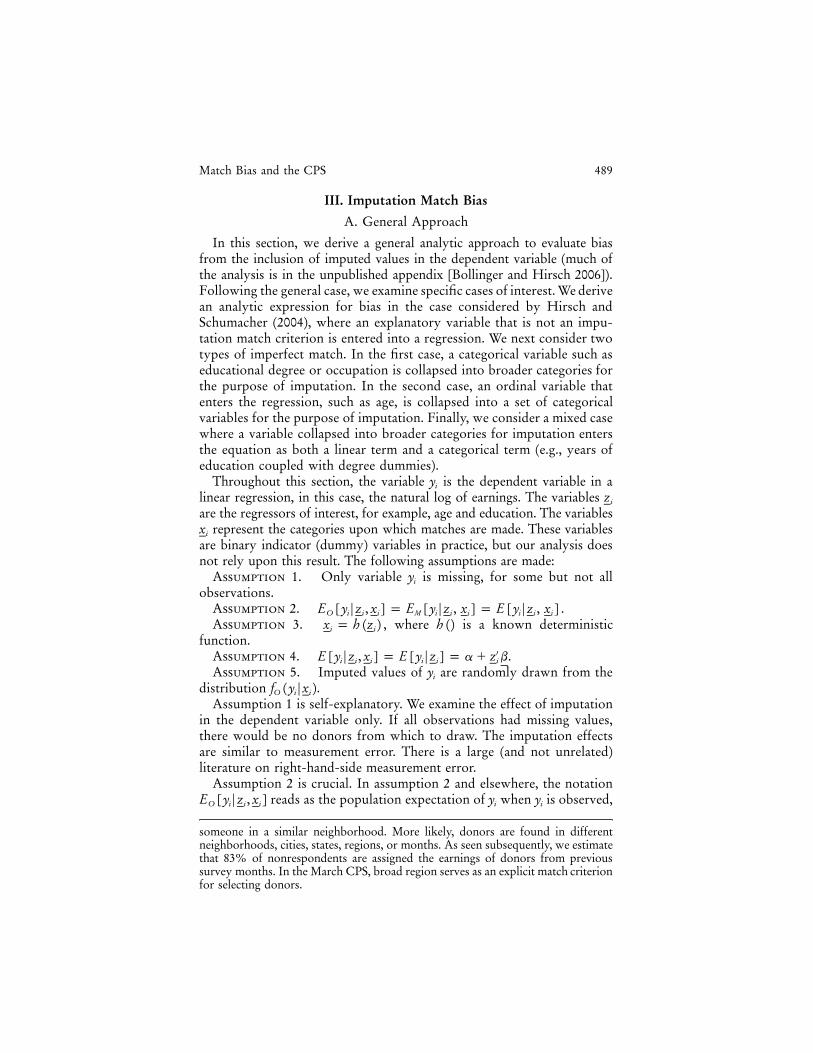
Parts a and b of figure 1 provide separate estimates of schooling returnsfor respondents and imputed earners. Estimates are from male and femalewage equations, using the same 1998–2002 CPS samples seen in the priorsection. Shown in the figures are log wage differentials for each schoolinggroup relative to earnings respondents with no zero schooling. Control

Fig. 1.—Schooling returns among male and female respondents and imputed earners,1998–2002. Estimates are from a pooled wage equation of respondents and imputed earnersusing the CPS-ORG for 1998–2002. The male sample size (pt. a) is 388,578—276,909 re-spondents and 111,669 with earnings allocated (imputed) by the Census. The female samplesize (pt. b) is 369,762—270,537 respondents and 99,225 with earnings allocated (imputed) bythe Census. The sample includes all nonstudent wage and salary workers, ages 18 and over.Shown are log wage differentials for each schooling group relative to earnings respondentswith no schooling. In addition to the education variables, control variables include potentialexperience (defined as the minimum of age minus years schooling minus 6 or years since age16) in quartic form, race-ethnicity (four dummy variables for five categories), foreign born,marital status (2), part time, labor market size (6), region (8), and year (4).

Match Bias and the CPS 505
variables are listed in the figure note. Variables that most clearly reflectpostmarket outcomes (occupation, industry, union status, etc.) are notincluded.17 The basic story seen in the figures is identical for women andmen. The earnings of respondents (shown by “diamonds”) increase fairlysteadily with schooling level. In contrast, imputed earnings among non-respondents (“squares”) are essentially flat in the low education categoryand increase only slightly within the middle and high education categories.Failure to account for match bias leads to a downward bias in estimatesfor those at high education levels within each group and an upward biasfor those with low education within each group. It leads to upwardlybiased “jumps” in earnings as one moves across categories, specificallythe movement from high school dropout to GED and from an associate’sdegree to a BA.
The GED results warrant examination. Here, upward match bias issevere, because the GED is the lowest education level within the middleeducation match category. Based on the sample of earnings respondents,the earnings gain for a male GED recipient relative to men who stop at12 years of high school without a degree is a modest .036.18 The samedifferential for imputed earners is an incredible .241 log points, as is seenin part a of figure 1 as the large jump between the Sch_12 and GED“squares.” A standard wage equation using an uncorrected full samplewould find a misleadingly large .087 wage gain for the GED (not shown),more than double the .036 estimate found for respondents. Similarly,imputation bias distorts the observed wage advantage for regular highschool graduates as compared to GED recipients. The standard biasedestimate indicates a .042 GED wage disadvantage, substantially smallerthan the .072 GED disadvantage found among those with observed earn-ings. Among the sample of imputed earners, little wage difference is foundbetween those with GEDs and standard diplomas. The story seen forwomen is extremely similar. As emphasized by Heckman and LaFontaine(2006, in this issue ) and in previous literature, GED estimates are alsobiased upward by unobserved heterogeneity, a bias that we do not addresshere.19
17 We do not interpret schooling parameters, even those corrected for match bias,as causal effects. Among other things, the estimates do not account for ability biasor reporting error in education.
18 The CPS provides information on years of schooling completed prior to receiptof the GED. We do not use that information here, but we do use it in our subsequentanalysis of “sheepskin” effects.
19 Heckman and LaFontaine (2006, in this issue) provide a detailed analysis ofthe GED and imputation bias, including a critique of misleading results found inClarke and Jaeger (2006). Using the post-1998 CPS, they show that the positiveeffect of the GED on earnings is small once one omits imputed earners or, alter-natively, uses the GED as an imputation match criterion. Based on additional analysisusing the NLSY (National Longitudinal Survey of Youth) and the NALS (National

506 Bollinger/Hirsch
Equally startling examples of bias from imperfect matching are seenamong workers with professional degrees and PhDs. Match bias in thiscase is downward, owing to these groups having the highest educationlevels within the “high” schooling category but being matched primarilyto donors with the BA as their terminal degree. Estimates from the re-spondent sample reveal a large .355 log point wage advantage among menwith professional degrees as compared to men with BA degrees. Basedon a standard full sample without correction, the wage advantage is .241,attenuation being 32%. The bias is similarly large for women, with aprofessional/BA degree wage advantage of .444 log points among earningsrespondents versus .296 using the full sample, attenuation of 33%. Asimilar pattern of bias is readily evident for those with PhD degrees.
In short, match bias due to incomplete matching on education flattenswage-schooling profiles within educational match categories, while itsteepens the jump in wages between categories. Depending on the specificlevel of schooling attainment being examined, bias can range from smallto very large. In a subsequent section, we examine a mixed model withan ordinal schooling variable and categorical degree variables (sheepskineffects).
F. Imperfect Match on Ordinal Variables
1. Theory
Here we consider a simplified case where a scalar ordinal variable, suchas age, enters a regression linearly but is reduced to two categories forpurposes of the imputation match. We use the term ordinal, but the anal-ysis applies equally well to ordered categorical variables and cardinalvariables. Indeed, age (or experience) is typically treated as cardinal. Forsimplicity, this section assumes missing at random, but similar results holdfor less restrictive assumptions. The specific structure is
[ ]E yFz pa�bzi i i
and
1 if z 1 z*ix p .i {0 if z ≤ z*i
Given this simple structure, it follows then that
[ ] [ ] [ ] [ ]E yFx pa�bE zFx p 0 �b E zFx p 1 �E zFx p 0 x .( )i i i i i i i i i
Adult Literacy Survey), which permits an accounting for ability bias, the authorsconclude that the remaining effects of the GED seen in the CPS are unlikely to becausal.

Match Bias and the CPS 507
Substitution gives
[ ] ( ) [ ]E yFx , z pa� 1 � p bz � pb(E zFx p 0s i i i i i i
[ ] [ ]� E zFx p 1 �E zFx p 0 x ).( )i i i i i
Then the linear projection of on gives an intercept ofy zi i
2( ) [ ]a p a � b p 1 � R E z( ) i
and a slope coefficient of
2( )b p b 1 � p 1 � R ,( )
where is the squared correlation between and The slope coefficient2R z x .i i
is attenuated by the proportion p imputed, mitigated in part by correlationbetween the information in match variables and the nonmatch elementsxi
of . This result generalizes to multiple categories and to the case ofzi
quadratic age: the quadratic profile is flattened relative to the true profilewhen imputed values are included.
Maintaining the assumption of missing at random, these results can beextended to the case where additional match characteristics are includedin the regression. As with the previous case, all coefficients are biased.
2. Evidence: Wage-Age Profiles
As seen above, match bias resulting from imperfect matching arises inestimates of earnings profiles with respect to age (or potential experience).In the CPS, nonrespondents are matched to the earnings of donors in sixage categories: ages 15–17, 18–24, 25–34, 35–54, 55–64, and 65 and over(our analysis includes nonstudent workers, 18 and over). Thus, the slopesof profiles are flattened within age categories, with jumps in earningsacross categories. A simple way to illustrate the bias is to estimate linearwage-age profiles within each of the age categories using the respondentand imputed samples. We use a specification with largely “premarket”demographic and schooling variables, plus location and year controls.These results are shown in table 3.
The most notable bias is for young workers, whose wage-age profilesare steep. Focusing first on men, annual wage growth among respondentsis .041 for ages 18–24 and .028 for ages 25–34. Wage growth seen amongthose with imputed earnings is far lower, .006 for ages 18–24 and .004for ages 25–34. Wage growth is low in the 35–54 age interval, .005 in therespondent sample versus close to zero in the imputed sample. In the twooldest age categories, inclusion of imputed earnings causes wage declineto be understated. Identical patterns are seen for women, although overallwage-age growth is lower than for men (we observe wage growth withrespect to age and not accumulated work experience). Whereas female

508 Bollinger/Hirsch
Table 3Wage-Age and Wage-Experience Profile Estimates
Men Women
Linear wage growth per year within age groups:Respondents:
18–24 .041 .02925–34 .028 .02035–54 .005 .00255–64 �.021 �.01165 plus �.013 �.010
Imputed earners:18–24 .006 .00125–34 .004 .00235–54 .000 .00055–64 �.007 �.00265 plus �.003 .004
Quadratic potential experience profiles:Respondents:
Exp .039 .025Exp2/100 �.068 �.044
Imputed earners:Exp .035 .023Exp2/100 �.057 �.039
Pooled sample:Exp .038 .024Exp2/100 �.065 �.042
Sample sizes:Respondents 276,909 270,537Imputed earners 111,669 99,225Pooled sample 388,578 369,762
Note.—The sample is all nonstudent wage and salary workers, ages 18 and over, from theCPS-ORG, 1998–2002. Control variables include a full set of education dummies, demo-graphic variables, region, city size, and year. Specifications including age variables do notinclude potential experience.
respondents display annual wage growth of .029 for ages 18–24 and .020for ages 25–34, growth using the imputed sample is effectively zero.
A more general way to illustrate the bias is to include a full set of agedummies and to estimate wage-age profiles for respondents and nonres-pondents. These results are shown separately for men and women, re-spectively, in parts a and b of figure 2. Imputed earners exhibit substantialflattening of wage-age profiles within each age category, the bias beingmost serious for ages 18–24 and 25–34 when wage growth is highest. Inthe imputed worker sample, large wage jumps are observed between ages24 and 25, between ages 34 and 35, and, going in the opposite direction,between ages 64 and 65. There is no jump between ages 54 and 55, sincethe weighted means of assigned donor earnings are similar in the adjacentage intervals.
Does inclusion of imputed earners greatly distort coefficients on po-tential experience in a Mincerian wage equation? The short answer is “alittle.” The most typical wage equation includes potential experience as

Match Bias and the CPS 509
Fig. 2.—Male and female wage-age profiles (pts. a and b, respectively). Same samples as infigure 1. Shown are log wage differentials at each age relative to earnings of respondents whoare age 18. In addition to the education dummies, control variables include race-ethnicity (fourdummy variables for five categories), foreign born, labor market size (6), region (8), and year(4).
a quadratic.20 In a male wage equation, respondents have a quadratic logwage profile of .039 and �.068 (to rescale coefficients, is divided2Expby 100). Estimates for the imputed sample produce a flatter profile, .035and �.057. Estimating the profile using the full sample without correction,
20 Murphy and Welch (1990) and Lemieux (2006) make strong arguments for useof higher-order terms (e.g., up to a quartic) in the Mincerian wage equation, as wasdone in the regressions shown in tables 2 and 4 and fig. 1.

510 Bollinger/Hirsch
coefficient estimates are .038 and �.065, a profile slightly flatter than theone observed for respondents. Uncorrected standard errors (not shown)are much higher when imputed earners are included. An identical qual-itative pattern is seen for women.
In short, bias due to imperfect matching causes wage patterns within andacross age-match categories to be meaningless among imputed earners. Fail-ure to account for this form of match bias has a modest effect in mostapplications, but it should not be ignored in analyses of earnings-experience(age) profiles, particularly those focusing on wage growth among youngworkers.
G. Mixed Case: Imperfect Matching with Ordinal and MultipleCategory Variables
1. Theory
Education provides an important example of a mixed case. Some re-searchers observe that, in addition to a linear return to years of education,there are “sheepskin” effects, which result in jump discontinuities in theearnings-education profile. We examine the implications of match bias forthis type of specification. Let be a dummy variable and let be anz z1i 2i
ordinal variable, with
1 if z 1 z*2iz p .1i {0 otherwise
We assume that
E yFz p a�b z � b zi i 1 1i 2 2i[ ]—
and that That is, the single match characteristic is the dummyx p z .i 1i
variable. For simplicity, we assume MAR for this result. Following ourunpublished appendix (Bollinger and Hirsch 2006) and recognizing that
the bias terms for the two slope coefficients will bex p z ,i 1i
�1 [ ]V C 0 E z z � E z Fz b( )[ ]1 1i 2i 2i 1i 1 ,[ ] [ ][ ][ ]C V 0 E z z � E z Fz b( )[ ]2 2i 2i 2i 1i 2
where is the variance of is the variance of , and C is theV z , V z1 1i 2 2i
covariance between and The term , whilez z . E [z (z � E [z Fz ])] p 01i 2i 1i 2i 2i 1i
the term is the variance of conditional onE [z (z � E [z Fz ])] z z .2i 2i 2i 1i 2i 1i
Define as the squared correlation between and , and note that2R z z1i 2i
. Then the above bias equation can2E [z (z � E [z Fz ])] p V (1 � R )2i 2i 2i 1i 2
be written as
�1V C 0 0 b1 1 .2[ ] [ ][ ]( )C V 0 V 1 � R b2 2 2

Match Bias and the CPS 511
Evaluating leads to the following expressions for the bias from the leastsquares projection:
Cb p b � p b ,1 1 2V1
( )b p b 1 � p .2 2
Here we see that the degree effect will be overstated (since by definitionof and the covariance will be positive), while the year or marginalz z1i 2i
effect will be understated. Indeed, if there is no degree effect (if ),b p 01
its OLS estimate will still be positive while the marginal effect will beunderstated. It must be kept in mind that the presence of other variableswill alter these results.
2. Evidence: Sheepskin Effects and Linearity
A common approach in estimating the returns to schooling is to as-sume linearity and to include a single schooling variable measuring yearsof school completed. The schooling coefficient represents the percentage(log) wage gain associated with an additional year of schooling (seeMincer [1974], Willis [1986], and subsequent literature for assumptionsnecessary to interpret this as a rate of return). A related approach in-cludes indicators for completed degrees, measuring separately the effectof the sheepskin on earnings. This approach can be informative (but notdecisive) in determining the extent to which education increases humancapital and the extent to which it provides some verifiable signal ofinnate human capital or motivation. In the extreme (and ignoring com-plicating factors), if education is exclusively human capital enhancement,then the coefficients on the degree completion indicators should ap-proach zero and years of schooling should measure the full humancapital effect. If education provides only a signaling mechanism, thenthe coefficient on years schooling should approach zero and only thedegree effects should matter.21
Table 4 provides estimates of a model with these mixed education var-iables. The sample is restricted to the range of data over which we canclearly distinguish between years of schooling and degree. We omit therelatively few workers with less than 9 years of schooling or with pro-fessional and PhD degrees for whom separate information on years
21 If unmeasured ability differences lead degree recipients to acquire more humancapital per year of schooling than do nonrecipients, estimates of degree effects willbe positively biased.

512 Bollinger/Hirsch
Table 4Estimated Schooling and Sheepskin Effects, 1998–2002
FullSample Imputed Respondents
Respondents(IP Weighted)
FullSample
(Corrected)
Men:School (years completed) .036 .022 .042 .043 .046GED .119 .251 .067 .067 .068High school .136 .230 .097 .094 .092Associate’s degree .190 .270 .156 .151 .160BA .367 .549 .294 .287 .268Master’s .414 .587 .345 .337 .335
N 359,564 103,476 256,088 256,088 359,564Women:
School (years completed) .048 .030 .054 .056 .062GED .129 .236 .091 .093 .082High school .137 .224 .104 .104 .088Associate’s degree .237 .290 .215 .213 .214BA .368 .562 .297 .293 .252Master’s .440 .595 .382 .375 .347
N 353,585 95,120 258,465 258,465 353,585
Note.—The sample is drawn from the CPS-ORG, 1998–2002. It includes all nonstudent wage andsalary workers, ages 18 and over, with between 9 years of schooling and a master’s degree (omitted arethose with schooling of less than 9 years, those with professional degrees, and PhDs). Control variablesinclude a full set of demographic variables, region, city size, and year. The full sample includes both therespondent (observed) and imputed (missing) samples with Census imputation. Corrected estimates arebased on the full sample and the general bias correction shown in the text. The IP-weighted columnreports least squares estimates from the respondent sample reweighed by the inverse probability that anindividual’s earnings are reported.
schooling is not provided.22 Estimates are provided using the full samplewith Census imputations and no bias correction (the standard approach),the respondent (“observed”) sample, the observed sample with inverseprobability weighting (IPW), and the full sample using the general cor-rection measure derived in Section III.C.
School is the measure of years of schooling completed. The full sampleestimate for men suggests a rate of return of .036 (in log points) for ayear of schooling, holding degree constant. The estimate on the observedsample is .042 absent weights and .043 reweighted to adjust for a changedsample composition. The corrected full sample estimate is .046, a per-centage point larger than the uncorrected estimate. Some of the degreeindicators, absent correction, are very misleading. For example, the co-efficient on high school degree in the full sample is .136. The estimatesfrom the observed sample, the IPW observed sample, and the correctedfull sample are much smaller at .097, .094, and .092, respectively. Similarly,
22 MA recipients designate their program as a 1, 2, or 3� year program. Infor-mation on additional years schooling is provided for those with some college andno degree and for BA degree recipients with graduate course work but no degree.Those with some college but no postsecondary degree are coded as having receiveda regular high school diploma (information on the GED is provided only for thosewithout education beyond high school).

Match Bias and the CPS 513
the estimated effect of a GED (years constant) is overstated due to matchbias. The full sample estimate places the value of a GED at .119, whilethe observed, IPW observed, and full corrected sample estimates are only.067, .067, and .068, respectively.23
The results for women follow a similar pattern. The full sample returnestimate of .048 is less than estimates from the observed sample of .054,the reweighted observed sample of .056, and the corrected full sample of.062. The GED full sample estimate of .129 compares to estimates of .091,.093, and .082 from the unweighted observed, IPW observed, and cor-rected full samples. Estimates of the value of a high school degree arevery similar to those for men.
The results confirm that imperfect group matching using the Censusimputation procedure biases rate of return estimates, trivially for someschooling groups but substantially for others. In a sheepskin model, theCensus imputation tends to understate the returns to years of schoolingwhile generally overstating degree effects. Sheepskin effects are still evi-dent, but these are less pronounced than those seen with observed Censusearnings or from estimates corrected for match bias.
IV. Dated Donors
Earnings nonrespondents are assigned the nominal earnings of the do-nor who is the most recent respondent with an identical mix of matchattributes. During the 1994–2002 period, the Census match procedureincluded 14,976 cells or combinations of match characteristics. For matchcells with a relatively uncommon mix, donor earnings may be relativelydated, biasing downward imputed earnings owing to nominal and realwage growth. Stated alternatively, the survey month can be considered awage determinant in that, for nonrespondents, is imperfectly mappedzi—from .xi—
How serious is the dated donor problem? The Census does not recordthe “shelf age” of donor earnings assigned to nonrespondents. To assessthis issue, one must approximate Census hot deck methods and measurethe datedness of donor earnings. Our analysis begins with all employedwage and salary workers, ages 18 and over, from the December 2002 CPS.That month’s file contains 4,759 nonrespondents. Some of these individ-uals will be matched to donor earnings in the current month, while mostwill reach back to donors in previous months and years. Each nonres-pondent in December 2002 is given a unique match number correspondingto the 14,976 possible combinations of match attributes. Likewise, po-
23 Note that these estimates account for the years of schooling completed by GEDrecipients (mostly 9–12 years). Prior estimates of a GED effect, drawn from fig. 1,did not include a separate years schooling variable and compared GED recipientsto those with 12 years schooling but no degree.

514 Bollinger/Hirsch
Fig. 3.—Dated donors: CPS cumulative imputation match rate for current and prior monthdonors. Cumulative monthly match rates of CPS-ORG nonrespondents in 2002 to 1998–2002potential donors. Period 0 represents donor matches in the current survey month, while periodn represents donor matches in the nth prior month. Period 60� figures represent all nonres-pondents not finding a donor match during the period 1998–2002.
tential donors (respondents) in 60 monthly CPS earnings files (December2002 back to January 1998) are assigned attribute match numbers on thesame basis. We first examine whether at least one donor match exists foreach nonrespondent in December 2002. Those not finding a donor areretained, and a search for a donor in November 2002 is executed. Thisprocess continues back to January 1998. In order to increase the size andrepresentativeness of the nonrespondent sample, we conduct the identicalanalysis for nonrespondents during from January to November 2002. Thetotal number of nonrespondents during 2002 is 55,902.24
Cumulative match rates resulting from the donor match exercise areshown in figure 3. In the initial month, just 17.3% of 2002 nonrespondentsfind a same-month donor.25 Reaching back 1 month, an additional 16.8%
24 For ease of programming, nonrespondents during each month of 2002 aretreated as if they were December nonrespondents. That is, for each 2002 nonres-pondent, we first search for matching donors in December 2002, and then we reachback in time as far as January 1998.
25 To approximate the Census match rate in the initial month, the donor pool isconstructed by taking a 50% random sample of December 2002 respondents. TheCensus searches for donors among those who are listed in the file layout prior tothe nonrespondent. Thus, nonrespondents at the beginning of the December 2002file are assigned donors from November 2002 or earlier, whereas nonrespondents

Match Bias and the CPS 515
are matched, followed by 11.5% and 8.3% reaching back 2 and 3 months.Within these first 4 survey months (the sample month plus 3 monthsback), over half (53.9%) of all nonrespondents are assigned donor earn-ings. Those not finding matches have decreasing match hazards (proba-bilities of finding a match) in subsequent months. Even after 5 years,reaching back 59 months from month zero to January 1998, 2.85% ofnonrespondents remain without an earnings assignment and are assigneddonor earnings in excess of 5 years old. In figure 3, we add the residualmonthly match rate of 2.85% to the prior month labeled 60 plus.
Beginning in 2003, the number of occupation categories in the Censusmatch algorithm was reduced from 13 to 10, reducing the number of hotdeck cells from 14,976 to 11,520. In order to see how this affects donordatedness, we provide an analysis matching the 17,864 earnings nonres-pondents in the January–April 2004 period to donors beginning in April2004 and reaching back to January 2003 (the first month with the newoccupation codes). We find little change in average donor datedness.Whereas 53.9% of the 2002 nonrespondents found donors during thecurrent or 3 previous months, the corresponding number for the Janu-ary–April 2004 nonrespondents is 53.1%. Reaching back 15 months,84.0% of the 2002 nonrespondents found a match; the correspondingnumber for 2004 respondents is 83.4%. We conclude that donor datednesshas not appreciably changed as a result of the revised occupational matchcategories beginning in 2003.
How serious is the problem of dated donor earnings? Combining in-formation on average donor age with the rate of wage growth, one canestimate the downward bias in average earnings. To calculate mean donorage one must assume an average match date for the nonrespondents whohave failed to find a match in the previous 5 years. For the 2002 sampleof nonrespondents, we assume that the 2.85% not matched going backto January 1998 would on average find a match in 6 additional months.Using this assumption, the average age or datedness of all donor earningsis 8.6 months, or nearly three-quarters of a year, substantially larger thanthe median age of 3 months (the current month and 3 months back).26 Ifnominal wage growth were, say, 3% annually, this would imply that theaverage earnings of donors are understated by 2.25%. With approximately30% of the CPS sample being nonrespondents, the CPS understates av-erage earnings by .675% (three-quarters of a year times 3% annual wage
at the end of the file can be matched to the full month donor sample. We approximatethis by using a half donor sample in the initial month (and full samples thereafter).If we instead search through all December respondents for donors, the initial matchrate increases by several percentage points and the next month rate falls, with quickconvergence in subsequent months to the rates in fig. 3.
26 The estimate of an 8.6 month mean donor age is sensitive to the assumed averagematch date for those relatively few (2.85%) nonrespondents remaining unmatched.

516 Bollinger/Hirsch
growth times .30 proportion donors), or two-thirds of a percentage point.In 2004, average hourly earnings compiled from the CPS, including im-puted earners, is $17.69, 2.85% higher than the 2003 average of $17.20.Multiplying by .0064 (.75 times 2.85% times .30), earnings are understatedby $.11, with the true average wage closer to $17.80. This was a periodof modest nominal wage growth; the bias increases proportionately withthe growth rate.
Do dated donors affect wage gap estimates? To the extent that a “treat-ment” group of workers has more (less) dated donors than a comparisongroup, the treatment group wage gap will be understated (overstated).Comparisons of the average datedness of donors across various groupsof workers based on gender and race suggest that standard wage gapestimates in the literature have been affected little by bias from dateddonors.
Most CPS nonrespondents are matched to the nominal earnings ofdonors from prior months rather than the current month, causing earningsto be understated. The resulting bias for most labor market studies, how-ever, is modest and does not warrant serious concern. If nominal wagegrowth were to increase sharply in future years, this conclusion wouldwarrant reconsideration.
V. Conclusion
Match bias arising from Census earnings imputation is an issue of someconsequence, but it is not one that generally has been considered by laboreconomists. Given the assumption of conditional mean missing at random(CMMAR), this article derives a general analytic solution that measuresmatch bias in its multiple forms. Bias is of first-order concern in studiesestimating wage gaps with respect to attributes that are not Census matchcriteria (union status, foreign born, etc.). Attenuation in this case isroughly equal to the imputation rate, nearly 30% in recent CPS earningssurveys. Consistent estimates can be obtained from samples including onlyearnings respondents (weighted or unweighted) or from the full samplecorrected for match bias.
This article shows that earnings imputation also warrants concern wherethere is matching on an attribute but the match is imperfect (e.g., edu-cation, age, occupation). Matching across a range of values flattens esti-mated earnings profiles within match categories (say, low, middle, andhigh education), while creating jumps across categories. Such match biascan be modest or severe, leading to overstatement (e.g., returns to theGED) or understatement (e.g., returns to professional and doctoral de-grees). We also draw attention to rather subtle forms of match bias, forexample, understatement of imputed earnings due to the datedness ofdonors (also see Hirsch 2005).
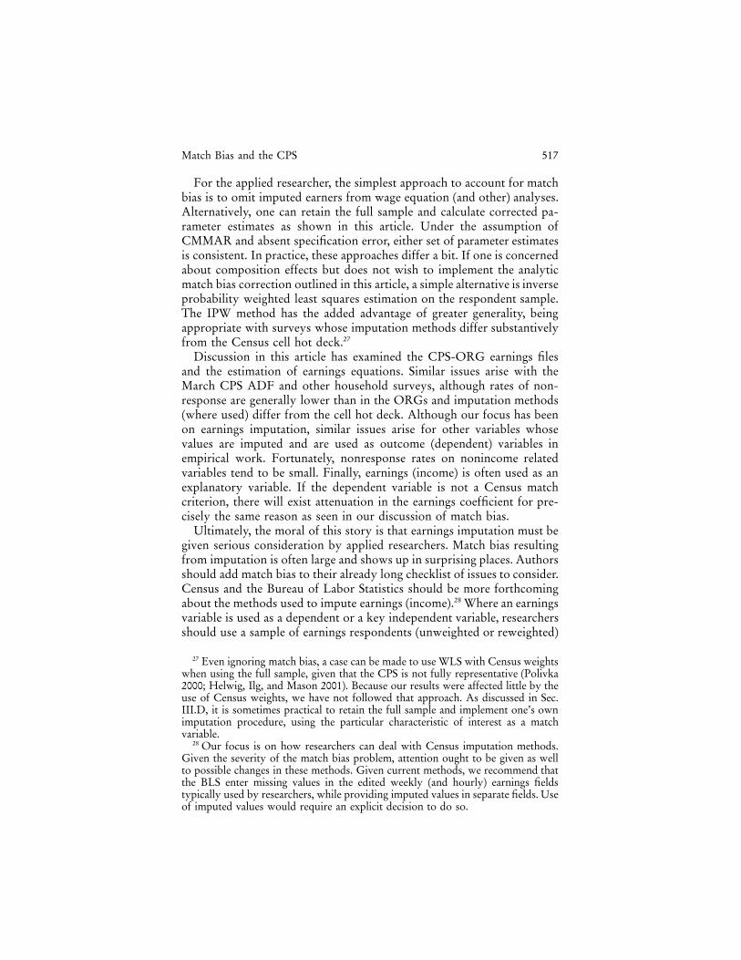
Match Bias and the CPS 517
For the applied researcher, the simplest approach to account for matchbias is to omit imputed earners from wage equation (and other) analyses.Alternatively, one can retain the full sample and calculate corrected pa-rameter estimates as shown in this article. Under the assumption ofCMMAR and absent specification error, either set of parameter estimatesis consistent. In practice, these approaches differ a bit. If one is concernedabout composition effects but does not wish to implement the analyticmatch bias correction outlined in this article, a simple alternative is inverseprobability weighted least squares estimation on the respondent sample.The IPW method has the added advantage of greater generality, beingappropriate with surveys whose imputation methods differ substantivelyfrom the Census cell hot deck.27
Discussion in this article has examined the CPS-ORG earnings filesand the estimation of earnings equations. Similar issues arise with theMarch CPS ADF and other household surveys, although rates of non-response are generally lower than in the ORGs and imputation methods(where used) differ from the cell hot deck. Although our focus has beenon earnings imputation, similar issues arise for other variables whosevalues are imputed and are used as outcome (dependent) variables inempirical work. Fortunately, nonresponse rates on nonincome relatedvariables tend to be small. Finally, earnings (income) is often used as anexplanatory variable. If the dependent variable is not a Census matchcriterion, there will exist attenuation in the earnings coefficient for pre-cisely the same reason as seen in our discussion of match bias.
Ultimately, the moral of this story is that earnings imputation must begiven serious consideration by applied researchers. Match bias resultingfrom imputation is often large and shows up in surprising places. Authorsshould add match bias to their already long checklist of issues to consider.Census and the Bureau of Labor Statistics should be more forthcomingabout the methods used to impute earnings (income).28 Where an earningsvariable is used as a dependent or a key independent variable, researchersshould use a sample of earnings respondents (unweighted or reweighted)
27 Even ignoring match bias, a case can be made to use WLS with Census weightswhen using the full sample, given that the CPS is not fully representative (Polivka2000; Helwig, Ilg, and Mason 2001). Because our results were affected little by theuse of Census weights, we have not followed that approach. As discussed in Sec.III.D, it is sometimes practical to retain the full sample and implement one’s ownimputation procedure, using the particular characteristic of interest as a matchvariable.
28 Our focus is on how researchers can deal with Census imputation methods.Given the severity of the match bias problem, attention ought to be given as wellto possible changes in these methods. Given current methods, we recommend thatthe BLS enter missing values in the edited weekly (and hourly) earnings fieldstypically used by researchers, while providing imputed values in separate fields. Useof imputed values would require an explicit decision to do so.

518 Bollinger/Hirsch
or provide corrected full sample coefficient estimates. Inclusion of im-puted earners absent bias correction should not occur, absent a persuasiveargument for doing so. Such arguments are not easy to make.
References
Aigner, Dennis J. 1973. Regression with a binary independent variable sub-ject to errors of observation. Journal of Econometrics 1, no. 1:49–59.
Angrist, Joshua D., and Alan B. Krueger. 1999. Empirical strategies inlabor economics. In Handbook of labor economics, vol. 3A, ed. OrleyC. Ashenfelter and David Card, 1277–1366. Amsterdam: Elsevier.
Black, Dan A., Mark C. Berger, and Frank A. Scott. 2000. Boundingparameter estimates with non-classical measurement error. Journal ofthe American Statistical Association 95 (September): 739–48.
Bollinger, Christopher R. 1996. Bounding mean regressions when a binaryregressor is mismeasured. Journal of Econometrics 73 (August): 387–99.
Bollinger, Christopher R., and Barry T. Hirsch. 2006. Appendix accom-panying “Match bias from earning imputation in the Current Popu-lation Survey,” Journal of Labor Economics 24 (July). Available at eitherhttp://gatton.uky.edu/faculty/bollinger/Workingpapers/jole_app.pdfor http://www.trinity.edu/bhirsch/jole_app.pdf.
Card, David. 1996. The effect of unions on the structure of wages: Alongitudinal analysis. Econometrica 64 (July): 957–79.
Clarke, Melissa A., and David A. Jaeger. 2006. Natives, the foreign-born,and high school equivalents: New evidence on the returns to the GED.Journal of Population Economics (forthcoming).
Groves, Robert M. 2001. Survey nonresponse. New York: Wiley.Groves, Robert M., and Mick P. Couper. 1998. Nonresponse in household
interview surveys. New York: Wiley.Heckman, James J., and Paul A. LaFontaine. 2006. Bias-corrected esti-
mates of GED returns. Journal of Labor Economics 24, no. 3:661–700.Helwig, Ryan T., Randy E. Ilg, and Sandra L. Mason. 2001. Expansion
of the Current Population Survey sample effective July 2001. Employ-ment and Earnings 48 (August): 3–7.
Hirsch, Barry T. 2005. Why do part-time workers earn less? The role ofworker and job skills. Industrial and Labor Relations Review 58 (July):525–51.
Hirsch, Barry T., and Edward J. Schumacher. 2004. Match bias in wagegap estimates due to earnings imputation. Journal of Labor Economics22 (July): 689–722.
Horowitz, Joel L., and Charles F. Manski. 1998. Censoring of outcomesand regressors due to survey non-response: Identification and esti-mation using weights and imputations. Journal of Econometrics 84(May): 37–58.

Match Bias and the CPS 519
———. 2000. Nonparametric analysis of randomized experiments withmissing covariate and outcome data. Journal of the American StatisticalAssociation 95 (March): 77–84.
Lemieux, Thomas. 2006. The “Mincer Equation” thirty years after School-ing, experience, and earnings. In Jacob Mincer, a pioneer of modernlabor economics, ed. Shoshana Grossbard. New York: Springer Verlag.
Lillard, Lee, James P. Smith, and Finis Welch. 1986. What do we reallyknow about wages? The importance of nonreporting and Census im-putation. Journal of Political Economy 94 (June): 489–506.
Little, Roderick J. A., and Donald B. Rubin. 2002. Statistical analysis withmissing data. New York: Wiley.
Mincer, Jacob. 1974. Schooling, experience, and earnings. New York: Co-lumbia University Press.
Molinari, Francesca. 2005. Missing treatments. Photocopy, Departmentof Economics, Cornell University (June).
Murphy, Kevin M., and Finis Welch. 1990. Empirical age-earnings profiles.Journal of Labor Economics 8 (April): 202–29.
Polivka, Anne E. 2000. Using earnings data from the Monthly CurrentPopulation Survey. Photocopy, Bureau of Labor Statistics (October).
Schafer, Joseph L., and Nathaniel Schenker. 2000. Inference with imputedconditional means. Journal of the American Statistical Association 95(March): 144–54.
Shao, J., and R. R. Sitter. 1996. Bootstrap for imputed survey data. Journalof the American Statistical Association 91 (September): 1278–88.
U.S. Department of Labor, Bureau of Labor Statistics. Various years.Median weekly earnings of full-time wage and salary workers by unionaffiliation, occupation and industry, Washington, DC. http://www.bls.gov/cps/cpsaat43.pdf.
———. 2002. Current Population Survey: Design and methodology. Tech-nical Paper 63RV, Bureau of Labor Statistics, Washington, DC (March).http://www.bls.census.gov/cps/tp/tp63.htm.
Willis, Robert J. 1986. Wage determinants: A survey and reinterpretationof human capital earnings functions. In Handbook of labor economics,vol. 1, ed. Orley C. Ashenfelter and Richard Layard. Amsterdam:Elsevier.
Wooldridge, Jeffrey M. 2002. Econometric analysis of cross section andpanel data. Cambridge, MA: MIT Press.
Wu, Lang. 2004. Exact and approximate inferences for nonlinear mixedeffects models with missing covariates. Journal of the American Statis-tical Association 99 (September): 700–709.