MAT334, Complex variables University of Toronto, Summer 2020
144
MAT334, Complex variables University of Toronto, Summer 2020 Nathan Carruth This document includes lecture notes, homework sets and solutions, term test and final assessment solutions, and background review material. It was typed up as the course progressed and has not been subsequently modified, so should be considered a rough draft. Comments or corrections can be sent to the author at [email protected]. The course was co-taught with Matthew Sourisseau, whose input is hereby gratefully acknowledged. All errors, inaccuracies, omissions, unnecessary additions, poor taste, etc., are my responsibility alone. Copyright c Nathan Carruth 2020. All rights reserved. May be freely copied and distributed for noncommercial purposes as long as this copyright notice is preserved.
Transcript of MAT334, Complex variables University of Toronto, Summer 2020

MAT334, Complex variables
University of Toronto, Summer 2020
Nathan Carruth
This document includes lecture notes, homework sets and solutions, term test and final assessmentsolutions, and background review material. It was typed up as the course progressed and has not beensubsequently modified, so should be considered a rough draft. Comments or corrections can be sent to theauthor at [email protected].
The course was co-taught with Matthew Sourisseau, whose input is hereby gratefully acknowledged. Allerrors, inaccuracies, omissions, unnecessary additions, poor taste, etc., are my responsibility alone.
Copyright c©Nathan Carruth 2020. All rights reserved. May be freely copied and distributed fornoncommercial purposes as long as this copyright notice is preserved.
MAT334, 2020. I, §1 [May 5] The Complex Plane Nathan Carruth
Summary:• We give a description of the complex number system.• We then give a description of the complex plane and indicate why it is something which might be useful.
I. INTRODUCTION TO THE COMPLEX PLANE
1. Complex numbers. We probably saw complex numbers for the first time when we learned howto solve quadratic equations. For example, the equation
x2 = −1
has no solution over the real numbers. It turns out to be useful in algebra, and even more in analysis,to extend our number system by including an extra quantity, written i, which behaves exactly like a realnumber except that it has the property
i2 = −1. (1)
A general number in our new number system can be written in the form a+ bi, where a and b are arbitraryreal numbers,1 and we require that these numbers satisfy all of the standard rules of algebra, augmented byequation (1). Thus, for example, the product of two complex numbers is given by
(a+ bi)(c+ di) = ac+ bi · c+ a · di+ bi · di = ac+ bci+ adi+ bdi2 = ac− bd+ (bc+ ad)i.
(As shown here, whenever we write out a complex number we always combine real and imaginary termswhen possible.)
We generally use the letters z and w to denote complex numbers, and x and y to denote real numbers.We let C denote the set of all complex numbers. If z = a+ bi is a complex number, we call a the real partof z and b the imaginary part of z, and write a = Re z, b = Im z. Two complex numbers a + bi and c + diare equal if and only if their real and imaginary parts are equal.2
To every complex number a+ bi there corresponds another complex number known as its conjugate andgiven by a− bi.3 If z is any complex number, we write z for its conjugate. The conjugate will be seen laterto have many uses, but for the moment we note its use in finding inverses. First, note that if z = a+ bi, then
zz = (a+ bi)(a− bi) = a2 − (bi)2 = a2 + b2.
Thus if a+ bi 6= 0, then
1
a+ bi=
1
a+ bi· a− bi
a− bi=
a− bi
a2 + b2=
a
a2 + b2− i
b
a2 + b2,
which is defined since a+ bi 6= 0 implies that at least one of a and b is nonzero, so a2 + b2 > 0. This is thedesired formula for the inverse of a complex number.
See Goursat, §1.2. The complex plane. If z is any complex number, it determines two real numbers Re z and
Im z, and is in turn uniquely determined by these two numbers. This suggests that, just as we may think ofarbitrary real numbers as points on the real number line, we may think of arbitrary complex numbers as pointsin the complex plane. Specifically, given a plane with perpendicular axes which we call x and y, we associatewith any complex number z the point in this plane whose x-coordinate is Re z and whose y-coordinate isIm z. While complex numbers are per se abstract objects without any direct concrete significance, thisassociation allows us to think and speak of them as points in the plane. We shall do this whenever it seems
1 Whenever we write an arbitrary complex number as a+ bi, it will always be assumed that a and b arereal.
2 This means that the set {1, i} is a basis for C considered as a real vector space.3 We remind the reader that the presence of a + or − in front of a quantity does not guarantee the
resulting sign; in other words, +b can be negative and −b can be positive, and both will be respectivelywhen b is negative.
1
MAT334, 2020. I, §2 [May 5] The Complex Plane Nathan Carruth
convenient; thus we shall speak of “the point a + bi”, etc., when more carefully we should say “the pointcorresponding to the complex number a+ bi”.
Given the foregoing, it is clear that the point corresponding to the conjugate of a complex number a+biis simply the reflection in the x-axis of the point corresponding to a+ bi.
The foregoing connection between complex numbers and points in a plane, while it may be interesting,would not be particularly useful if the geometric properties inherent in the Euclidean plane were not some-how related to algebraic or analytic properties of the complex numbers its points represent. We shall seethroughout this course that there are in fact many and deep connections between the geometry of the planeon the one hand and the algebraic and analytic properties of complex numbers on the other. Here we shallindicate one example.
EXAMPLES. One simple example is as follows. Suppose that z = a + bi and w = c + di are any twocomplex numbers. Then clearly
zw = (a− bi)(c+ di) = ac+ bd+ i(ad− bc).
Now if we think of the vectors (corresponding to the points) corresponding to a+bi and c+di, i.e., v = ai+bj,u = ci+dj, we see that their dot product is v•u = ac+ bd while their cross product is v×u = (ad− bc)k; inother words, roughly, the real part of zw is the dot product of the vectors corresponding to z and w, whilethe imaginary part is their cross product.4 We shall see some other relations of this sort when we talk aboutderivatives of functions of a complex variable; it turns out that, when viewed as a vector field, the derivativeof the conjugate of such a function essentially encodes the divergence and curl of the vector field.5
As another, more interesting, example, let a+bi be any complex number, and consider the correspondingpoint in the plane. This point has polar coordinates (r, θ), where r is the distance from the origin to thepoint and θ is the angle from the positive x-axis to the ray from the origin passing through the point. Insymbols, this becomes
r =√
a2 + b2, cos θ =a√
a2 + b2, sin θ =
b√a2 + b2
a = r cos θ, b = r sin θ
Note that θ is only defined up to a multiple of 2π: the two polar coordinate expressions (r, θ) and (r, θ+2π)determine exactly the same point in the plane. We shall see shortly that for many important functions tobe continuous (in an appropriate sense) on the complex plane, there is no way around this ambiguity: it issimply something which must be dealt with.
Now suppose that c+ di is any other complex number which satisfies c2 + d2 = 1: this means that thepoint corresponding to c + di lies on the unit circle. If we let (r0, θ0) denote the polar coordinates of thispoint, then we have r0 = 1, while θ0 satisfies cos θ0 = c, sin θ0 = d.6 Now applying basic trigonometricidentities, we obtain
(a+ bi)(c+ di) = ac− bd+ i(ad+ bc)
= r cos θ cos θ0 − r sin θ sin θ0 + i(r cos θ sin θ0 + r sin θ cos θ0)
= r cos(θ + θ0) + ir sin(θ + θ0)
= r [cos(θ + θ0) + i sin(θ + θ0)] ,
from which it is evident that the point corresponding to the product (a + bi)(c + di) is simply that corre-sponding to a+ bi rotated counterclockwise by the angle θ0!
4 It turns out that there is a four-dimensional extension of the real numbers called the quaternions, whichcontain the complex numbers, and which in some sense generalises results of this sort to full three-dimensionalvectors. We shall not deal with these in this course, though, except for a few asides like this one.
5 While interesting, these examples are somewhat tangential to the main content of this course.6 If you are familiar with De Moivre’s theorem, it is useful to note that this means that c+ di = cos θ0 +
i sin θ0.
2
MAT334, 2020. I, §2 [May 7] Exponentiation Nathan Carruth
Summary:• We discuss another geometric interpretation of complex multiplication.• We then discuss taking powers and roots of complex numbers, and the geometric interpretation of theseoperations.We have just observed that multiplying a complex number by another complex number of unit modulus
is equivalent to rotating the original complex number by an angle equal to that of the second complexnumber. It turns out that multiplication by a general complex number can be viewed as the composition ofa rotation and an isotropic scaling. Let us see how this works. Suppose that we have two complex numbers,
z = r(cos θ + i sin θ), w = r′(cos θ′ + i sin θ′).
Then their product comes out to be (the angular part is exactly analogous to what we saw at the end of thenotes of May 5)
zw = rr′(cos θ + i sin θ)(cos θ′ + i sin θ′)
= rr′(cos θ cos θ′ − sin θ sin θ′ + i[sin θ cos θ′ + cos θ sin θ′])
= rr′[cos(θ + θ′) + i sin(θ + θ′)];
(1)
in other words, the point corresponding to zw is exactly the point corresponding to z, rotated by θ′ andscaled by r′. This is the sense in which multiplication by a complex number is just a rotation and a scaling.(This is related to some of the problems on the review sheet!)
3. Exponentiation. We have seen that the affect of multiplication on the angular part of a complexnumber is just a rotation. What happens under exponentiation? Let z = r(cos θ+ i sin θ); then we see that,by the formula in (1) above,
z2 = z · z = r2(cos 2θ + i sin 2θ),
z3 = z · z2 = r(cos θ + i sin θ) · r2(cos 2θ + i sin 2θ) = r3(cos 3θ + i sin 3θ),
and so on, so that it is evident that for any positive integer m we have
zm = rm(cosmθ + i sinmθ).
To try to get some sense of what this means geometrically, let us first consider the case r = 1; then rm = 1for all m and we have simply
zm = cosmθ + i sinmθ.
Now any complex number of unit modulus is represented in the complex plane by a point on the unit circle,and completely determined by the angle between a ray drawn from the origin to that point and the positivex-axis, measured in a counterclockwise direction: this is just the number θ above. This formula then tellsus that the point corresponding to zm is also on the unit circle, but with an angle from the positive x-axisequal to m times that of the point corresponding to z. In other words, if we must traverse an angle θ toarrive at z, we must traverse an angle of mθ to arrive at zm.
Suppose now that we consider the affect of exponentiation on not just a single point on the unit circlebut rather an arc, say from θ = 0 to θ = θ0 for some θ0 > 0. The point corresponding to θ0, namelycos θ0+ i sin θ0, will be mapped by this exponentiation to cosmθ0+ i sinmθ0; and it is clear that every pointwith θ ∈ [0, θ0] will be mapped to a point with θ ∈ [0,mθ0]. Thus exponentiation simply stretches out theoriginal arc.
With this in mind, let us consider the affect of exponentiation on an angular wedge, namely on the setof all points (of whatever modulus) whose angle with the positive x-axis lies between 0 and θ0. Such a pointcan be written in the form z = r(cos θ+ i sin θ), where θ ∈ [0, θ0], and z
m = rm(cosmθ+ i sinmθ); from theforegoing, then, it is clear that this point will lie inside a ‘wedge’ (it may have an angle greater than π andhence not really be a proper ‘wedge’ anymore) extending from 0 to mθ0.
Now there is no particular reason to restrict the lower angular bound on the wedge to be 0; we may aswell consider a wedge [θ1, θ2]. The same logic shows that this will be mapped to a wedge [mθ1,mθ2].
In particular, if we consider the wedge from 0 to π and let m = 2, we see that the image underexponentiation is the ‘wedge’ from 0 to 2π, i.e., the entire complex plane. The same is true if we consider
3

MAT334, 2020. I, §3 [May 7] Complex derivatives Nathan Carruth
the wedge from 0 to 2π3 and let m = 3, and in general, if m is any positive integer, then the wedge from
0 to 2πm will be mapped to the entire complex plane by the map z 7→ zm. Similarly, the wedge from 2π
m to4πm will also be mapped to the entire complex plane, and so will the wedges from 2nπ
m to 2(n+1)πm for any
n = 0, 1, . . . ,m− 1.While we do not quite have all of the necessary tools to make the following picture precise, it provides
much useful intuition and I think is simple enough to understand. We may think of exponentiation by apositive integer as an endpoint in a process that starts with exponentiation by 1 (i.e., doing nothing!) andthen slowly increases the exponent through all real numbers until it reaches m. Under this kind of a map,the wedge from 0 to 2π
m (say) will be slowly stretched out (with the bottom edge, i.e., that along the x-axis,remaining fixed) until the outer edge finally reaches the x-axis. Under the same map, the wedge from 2π
m to4πm will behave slightly differently: the lower edge 2π
m also moves until it reaches the positive x-axis, while theupper edge 4π
m moves even faster so that by that point it has travelled one full 2π past the positive x-axis.Similar things can be said about the additional wedges.
What all of this means is that under exponentiation by a positive integer, the wedges 2πnm to 2π(n+1)
mare each rotated and stretched in such a way as to cover the entire complex plane exactly once.7 This meansthat each complex number is the image under the exponentiation map of exactly one point from each ofthese wedges. A little thought shows that this means that each complex number (except 0) has exactly mmth roots.
More precisely, suppose that z = r(cos θ + i sin θ) is some complex number. Now for each positive realnumber r there is exactly one positive real number R satisfying Rm = r, and we denote this unique positivereal mth root by r
1m . Given this, for n = 0, 1, . . . ,m− 1, let wn = r
1m
(cos θ+2πn
m + i sin θ+2πnm
); then clearly
wmn =
(
r1m
)m
(cos(θ + 2πn) + i sin(θ + 2πn))
= r(cos θ + i sin θ) = z,
so that each of the wn is an mth root of z. More specifically, if we assume that θ ∈ [0, 2π], then it is clearthat wn is in the nth of the above wedges. We note that wm = w0, and in general wn+km = wn for anypositive integer k. It can be shown that the wn are the only complex mth roots of z, and that z therefore hasexactly m distinct mth roots, as claimed. [The proof is not that hard: suppose that w = r′(cos θ′ + i sin θ′)is any mth root of z, i.e., that wm = z; this means that
r′m(cosmθ′ + i sinmθ′) = r(cos θ + i sin θ),
which means that r′m = r, i.e., r′ = r1m , and that there is an integer n such that mθ′ = θ+2nπ, which gives
θ′ = θm + 2nπ
m for some integer n. Now dividing n by m we can find integers q and r such that n = qm+ r
and r ∈ {0, 1, 2, . . . ,m− 1}; thus θ′ = θm + 2(qm+r)π
m = θm + 2qπ + 2rπ
m and this w is equal to wr .]
4. Complex derivatives. Cauchy-Riemann equations In first-year calculus we learned that thederivative of a real-valued function of a single real variable, if it exists, is given by the limit
f ′(x) = limh→0
f(x+ h)− f(x)
h.
In multivariable calculus, we learned about taking partial derivatives, which are derivatives in a singledirection at a time; we couldn’t take the derivative ‘with respect to a vector’ since we had no way of dividingby a vector.8 Those of you who have seen how derivatives of functions from Rn to Rm can be viewed aslinear operators between those spaces will still recall that the components of the matrix representations ofthose operators are still calculated as partial derivatives, i.e., even in that case we reduce back to the caseof a single function of a single variable.
7 Well, almost exactly once. To be precise we should only include one of the two edges, restricting theangle to lie in a half-open interval.
8 This is not entirely correct and there is in fact a nice way in which the gradient can be viewed as aderivative df
dr . But that is probably more of a notational shorthand than anything fundamental, unlike whatwe are about to do with complex numbers.
4

MAT334, 2020. I, §4 [May 7] Complex derivatives Nathan Carruth
In complex analysis, though, we can go further since we have a well-defined way of dividing by complexnumbers even though they are two-dimensional quantities (at least over R!). Let f : C → C be a complex-valued function of a complex variable, and consider the limit
limh→0
f(z + h)− f(z)
h,
where now h is allowed to be a complex number. Since h is complex, this means that we are taking atwo-dimensional limit. As we have learned in multivariable calculus, a two-dimensional limit can only existif directional limits from different directions exist and are equal (and it may fail to exist even then). Let usconsider what the above limit looks like in the two cases where we restrict h to go to zero along the realand imaginary numbers (in terms of the complex plane, this means that h goes to zero along the horizontaland vertical axes, respectively). First, let us write out f explicitly in terms of its real and imaginary partsas (writing z = x+ iy)
f(x+ iy) = P (x, y) + iQ(x, y),
and assume that all partial derivatives ∂P∂x ,
∂P∂y ,
∂Q∂x ,
∂Q∂y exist. If h = ∆x is real, the quotient inside the limit
becomes
f(x+ iy +∆x) − f(x+ iy)
∆x=P (x+∆x, y) + iQ(x+∆x, y)− [P (x, y) + iQ(x, y)]
∆x
=[P (x+∆x, y)− P (x, y)] + i[Q(x+∆x, y)−Q(x, y)]
∆x.
Since the partial derivatives ∂P∂x and ∂Q
∂x exist, in the limit as ∆x goes to zero this becomes
∂P
∂x+ i
∂Q
∂x.
This gives the original (two-dimensional) limit along the real axis. To find the limit along the imaginaryaxis, let h = i∆y (note the i!); then we obtain
f(x+ iy + i∆y)− f(x+ iy)
i∆y=P (x, y +∆y) + iQ(x, y +∆y)− [P (x, y) + iQ(x, y)]
i∆y
= −i{[P (x, y +∆y)− P (x, y)] + i[Q(x, y +∆y)−Q(x, y)]
∆y
}
,
so that since the partial derivatives ∂P∂y and ∂Q
∂y exist this becomes
−i{∂P
∂y+ i
∂Q
∂y
}
=∂Q
∂y− i
∂P
∂y.
For the full two-dimensional limit to exist, this must equal the limit along the real axis; thus we must have
∂Q
∂y− i
∂P
∂y=∂P
∂x+ i
∂Q
∂x,
which gives the celebrated Cauchy-Riemann equations
∂P
∂x=∂Q
∂y,
∂P
∂y= −∂Q
∂x.
To sum up: for a function f of a complex variable to have a derivative at a point, its real and imaginarycomponents P and Q must have partial derivatives at that point and those partial derivatives must satisfythe Cauchy-Riemann equations. It can be shown (see Goursat, §3) that if the partial derivatives of P and Qare also continuous at the point in question, then these conditions are sufficient in that f is then guaranteed
5

MAT334, 2020. I, §4 [May 7] Complex derivatives Nathan Carruth
to have a derivative at that point. Functions whose real and imaginary parts satisfy the Cauchy-Riemannequations but which do not have a derivative shall not concern us much in this course.
When f has a derivative at a certain point, by the foregoing that derivative is given by either of theexpressions
f ′(z) =∂P
∂x+ i
∂Q
∂x=∂Q
∂y− i
∂P
∂y.
Other equivalent expressions can also be derived; see Goursat, §3, equation (2).Let us consider a specific example of the foregoing.
EXAMPLES. Let us consider a very simple function:
f(z) = z2.
To find its real and imaginary parts, let z = x+ iy; then
f(z) = f(x+ iy) = (x + iy)2 = x2 + 2ixy − y2 = (x2 − y2) + i(2xy),
whence we see that its real and imaginary parts are, respectively,
P (x, y) = x2 − y2, Q(x, y) = 2xy.
We leave it as a worthwhile exercise to the reader to show that these do in fact satisfy the Cauchy-Riemannequations. Since they certainly have continuous partial derivatives, we see that f must have a derivative atany point z. The formulas above give this derivative as
f ′(z) = f ′(x+ iy) =∂P
∂x+ i
∂Q
∂x= 2x+ 2iy = 2z.
(This should not be a surprise, since we know from real-variable calculus that the derivative of x2 is 2x.) Inthis case, we can also derive this result directly, as follows:
f ′(z) = limh→0
f(z + h)− f(z)
h
= limh→0
(z + h)2 − z2
h= lim
h→0
z2 + 2zh+ h2 − z2
h= lim
h→0
2zh+ h2
h= lim
h→0(2z + h) = 2z.
This result turns out to be typical: most of the standard functions we are familiar with from calculuswhich have derivatives as functions of a real variable also have derivatives as functions of a complex variable,and the derivatives are the same. (There is a very good reason for this, which will become clearer throughoutthe course: it is tied up with the fact that most of the functions we deal with in calculus do not just have asingle derivative but are rather real analytic, i.e., are equal to their Taylor series expansions. Such functionsalways extend to differentiable functions of a complex variable, and this is one of the major links from realto complex variable theory.)
As a still elementary but slightly more complicated example, let us show that the power rule of elemen-tary calculus holds for functions of a complex variable, if we restrict ourselves to positive integer exponents.(It holds for more general exponents, too, at least away from z = 0, but that will require a separate treat-ment.) Thus let m be a positive integer, and define f(z) = zm. Then we have
limh→0
f(z + h)− f(z)
h= lim
h→0
(z + h)m − zm
h
= limh→0
1
h
(m∑
k=0
(m
k
)
zm−khk − zm
)
= limh→0
1
h
(
mzm−1h+m(m− 1)
2zm−2h2 + · · ·
)
= limh→0
(
mzm−1 +m(m− 1)
2zm−2h+ · · ·
)
= mzm−1,
since all terms in · · · have at least an h2 in them and hence must go to zero as h does. Thus we havef ′(z) = mzm−1, exactly as in the real-variable case.
6

MAT334, 2020. I, §4 [May 12 – 14] Differentiation rules Nathan Carruth
Summary:• We wrap up some loose ends from last time.• We discuss how differentiation rules from elementary calculus can be extended to the current setting.• We discuss multiple-valued functions and give a brief introduction to the notion of branch cut.
5. Harmonic functions. If a function f ′(z) has a derivative throughout a region, we say that it isanalytic in that region.9 From last time, we know that if we write f as
f(x+ iy) = P (x, y) + iQ(x, y),
then, assuming that P and Q possess continuous first-order partial derivatives, f will be analytic if P andQ satisfy the Cauchy-Riemann equations
∂P
∂x=∂Q
∂y,
∂P
∂y= −∂Q
∂x.
It turns out that these equations impose a very strong condition on P and Q, namely that they be harmonic,i.e., that they satisfy Laplace’s equation
∆f =∂2f
∂x2+∂2f
∂y2= 0.
Assuming that P and Q possess continuous second-order partial derivatives, this can be shown easily asfollows:
∂2P
∂x2+∂2P
∂y2=
∂
∂x
∂Q
∂y+
∂
∂y
[
−∂Q∂x
]
=∂2Q
∂x∂y− ∂2Q
∂y∂x= 0,
since under the above assumption the mixed partial derivatives of Q commute. The calculation for Q issimilar and we leave it to the reader as an exercise.
To summarise, then, we have the implication
f analytic =⇒ Re f, Im f harmonic.
Note that the reverse implication is false, since if P and Q are two harmonic functions there is in generalno reason at all to expect them to satisfy the Cauchy-Riemann equations. Note also that for us the termharmonic is applied only to real-valued functions of real variables; we do not speak of a function f of acomplex variable being harmonic. (We could define analytic for functions of a real variable – it is simplythat the function have a convergent power series representation – but we have not done so as we shall haveno particular need for this concept by itself.)
Harmonic functions are very important in many areas of physics and science, as they can be used todescribe temperature distributions, static electric fields, and steady-state fluid flows, for example. We shallsee later that one major application of complex variable theory lies in the use of analytic functions quaconformal maps to find solutions to Laplace’s equation in nontrivial geometries.
Given a harmonic function P , there is a harmonic function Q, unique up to an additive constant, suchthat f(x+ iy) = P (x, y) + iQ(x, y) is analytic. This is discussed in Goursat, §3, and also in §9 below.
6. Differentiation rules. We have already seen one example (at the end of §4 from last time) wherea differentiation rule from elementary calculus carried across essentially unchanged to the current setting. Itturns out that almost all of the differentiation rules from elementary calculus do also carry over to functionsof a complex variable: for example, the product rule and quotient rule do, since the proofs of those two
9 The word analytic, when applied to a real-valued function of a real variable, means that the functioncan be extended in a power series, i.e., that the Taylor series of the function converges to the function onsome interval. We shall show later that, for functions of a complex variable, existence of the derivativethroughout an appropriate region allows us to conclude that the function has derivatives of all orders, andthat the Taylor series about each point converges to the function on some disc. Thus our terminology isconsistent with the real-variable case.
7

MAT334, 2020. I, §6 [May 12 – 14] Roots and branch cuts Nathan Carruth
rules work equally well for complex independent variables as they do for real. This means that derivativesof rational functions (quotients of polynomials) can be found exactly as for functions of a real variable.
The chain rule also carries over to the current setting, as can be seen as follows. Suppose that f andg are analytic functions, and let z ∈ dom f be such that f(z) ∈ dom g. Then since f and g are analytic wehave
limh→0
f(z + h)− f(z)
h= f ′(z), lim
h′→0
g(f(z) + h′)− g(f(z))
h′= g′(f(z)).
Now the first relation can be rewritten in the following way:
limh→0
f(z + h)− f(z)− f ′(z)h
h= 0.
Let us write ǫ(h) = f(z + h) − f(z)− f ′(z)h, so that this result becomes limh→0ǫ(h)h = 0. Similarly let us
write ǫ′(h′) = g(f(z) + h′)− g(f(z))− g′(f(z))h′.10 Then we note that
limh→0
g(f(z + h))− g(f(z))
h= lim
h→0
g(f(z) + f ′(z)h+ ǫ(h))− g(f(z))
h
= limh→0
g′(f(z))[f ′(z)h+ ǫ(h)] + ǫ′(f ′(z)h+ ǫ(h))
h
= g′(f(z))f ′(z) + limh→0
[
g′(f(z))ǫ(h)
h+ǫ′(f ′(z)h+ ǫ(h))
h
]
;
but the limit of the first fraction is zero by what we know about ǫ(h), while the limit of the second is alsozero by what we know about ǫ(h) and ǫ′(h). Thus we have
d
dzg(f(z)) = g′(f(z))f ′(z),
exactly as we do in elementary calculus.We shall see shortly that, given appropriate extensions of the elementary transcendental functions of
calculus (the trigonometric, exponential, and logarithmic functions), the derivatives of all of these functionsare also what one would expect from calculus.
7. Roots and branch cuts. There is one class of functions which we have already extended to allcomplex numbers but whose derivatives we have not yet discussed, namely the roots. It turns out that a studyof these functions reveals a subtlety in functions of a complex variable which is not visible in functions of areal variable. Let us fix some positive integer m and consider mth roots. Recall that if z = r(cos θ + i sin θ)is any complex number, then the m complex numbers
wn = r1/m(
cosθ + 2πn
m+ i sin
θ + 2πn
m
)
all satisfy wmn = z. Now a function must have a unique value at a given point; thus if we wish to define an
mth root function we must have some way of choosing just one of these values for each point. At first sightit would appear that we could just take w0 and be done, but a bit more thought reveals that the situationis not quite that simple: for example, should z = r, for r a positive real number, be represented as
z = r(cos 0 + i sin 0), with mth root w0 = r1/m,
or as
z = r(cos 2π + i sin 2π), with mth root w0 = r1/m(
cos2π
m+ i sin
2π
m
)
?
10 For those who have seen this notation, we note that this is equivalent to saying that ǫ(h) = o(h) andǫ′(h′) = o(h′).
8

MAT334, 2020. I, §7 [May 12 – 14] Roots and branch cuts Nathan Carruth
If we are interested only in defining a function we may just choose one of these and be done. The problemwith that method, though, is that the resulting function will not be continuous across the real axis. Forsuppose that we make the requirement that θ ∈ [0, 2π), which corresponds to choosing the first of these twoexpressions. Let us consider the two limits
limh→0+
(cosh+ i sinh)1/m and limh→0−
(cosh+ i sinh)1/m.
For our mth root function to be continuous these two limits must be equal. But since we have required theangle θ to lie in the interval [0, 2π), we must rewrite the second number as
cos(2π + h) + i sin(2π + h)
(remember that here h is negative so 2π + h < 2π!), which means that the two limits become
limh→0+
(cosh+ i sinh)1/m = limh→0+
(
cosh
m+ i sin
h
m
)
= 1
and
limh→0−
(cos(2π + h) + i sin(2π + h))1/m = limh→0−
(
cos2π + h
m+ i sin
2π + h
m
)
= cos2π
m+ i sin
2π
m,
and these two expressions are clearly not equal unless m = 1 (when everything is quite trivial). A similarproblem would happen if we made the second choice above.
It turns out that the above difficulty is not just a result of our lack of cleverness: there is in fact no wayto define an mth root function which is single-valued and continuous on the entire complex plane. The basicidea is already contained in the foregoing. Suppose that f : C → C were a function of a complex variablesatisfying everywhere on C the formula
[f(z)]m = z,
and such that f(z) were continuous everywhere on C. Let us consider how f behaves on the unit circle.By our study of roots above, we know that there must be integer n ∈ {0, 1, 2, · · · ,m− 1} such that f(1) =cos 2πn
m + i sin 2πnm . Since f is continuous, for θ close to zero we must also have
f(cos θ + i sin θ) = cosθ + 2πn
m+ sin
θ + 2πn
m.
Now let us consider what happens when we gradually increase θ more and more. Clearly we must alwaysstill have
f(cos θ + i sin θ) = cosθ + 2πn
m+ sin
θ + 2πn
m,
since otherwise there would be a point where we would need to switch to a different value of n, and this wouldlead to a discontinuity in f (this could be shown analogously to how we argued above about discontinuityacross the real axis). Thus we can keep on going up until we get close to 2π. But if θ is very close to 2π theabove result gives
f(cos θ + i sin θ) = cosθ + 2πn
m+ sin
θ + 2πn
m;
but since we can consider θ < 0 as well as θ > 0, we also have
f(cos θ + i sin θ) = f(cos(θ − 2π) + i sin(θ − 2π)) = cosθ + 2π(n− 1)
m+ sin
θ + 2π(n− 1)
m,
a contradiction.
9

MAT334, 2020. I, §7 [May 12 – 14] Roots and branch cuts Nathan Carruth
Let us sum up what we have shown: No matter which choice of mth root we choose, if we continueit along a curve which encloses the origin, it will come back as a different root when we come back to theoriginal point. This phenomenon is actually quite common in the study of functions of a complex variable,and the origin is what is called a branch point of the mth root function. Far from being a failure of thetheory, it actually leads to very interesting new mathematical structures called Riemann surfaces, which wediscuss momentarily.
It turns out that if we wish to define an mth root function, there are two distinct ways to proceed. Firstof all, we could restrict the domain by removing (say) a ray from the origin to infinity from the domain ofthe function; for example, if we remove the positive real axis together with the origin, it is clear that we maymake any single choice of n and get a continuous mth root function on the remaining set. The same is true ifwe remove any other ray from the origin to infinity. In this setting, the ray we remove from the domain of fis termed a branch cut. See Goursat, §6, especially the discussion around Figure 5; see also some additionaldiscussion in §8 herein, below.
Goursat’s discussion of cutting the plane relates to the notion of a Riemann surface, which is part ofthe second possible route out of our difficulties, namely extending the domain to a so-called m-sheeted coverof the complex plane.11 This is rather complicated and we shall only sketch it. The idea is to consider thepoint 1 on the real axis as distinct from the point obtained by rotating it around the origin once, twice,thrice, . . ., m − 1 times, but as the same as what one gets by rotating m times.12 This gives m different‘sheets’ – in some sense, m different ‘copies’ of the complex plane – which are joined onto each other in somefashion (think of a spiral staircase which somehow ends up where it started); and we can then define themth root function by choosing root n on the nth of the sheets.
11 I don’t suppose anyone has studied covering spaces, but in case anyone has, let me just note that thiscorresponds to the m-sheeted cover of the unit circle by itself. The universal cover of the unit circle willshow up when we talk about the logarithm.12 If any of you have some familiarity with the notions of particle physics, you may recall that certain
elementary particles, such as the electron, are said to have spin-1/2, in that they must be turned aroundtwice to look the same (a most peculiar property!); that is exactly the same as what is going on here exceptthat for mth roots we must ‘turn around’ m times to look the same. While it has been too long since Istudied the Dirac equation to be sure of myself here, I doubt this is entirely a coincidence, as those of youwho have studied the Dirac equation will probably recall that it arises as a square-root of the Klein-Gordonequation.
10

MAT334, 2020. I, §7 [May 14] Roots and branch cuts, II Nathan Carruth
Summary:• We clarify some matters related to branch cuts.• We then fill in some points from the last set of lecture notes.• Finally, we introduce power series and discuss how to extend the exponential and logarithm to complexnumbers.
8. Roots and branch cuts, II. In the lecture notes from Tuesday, §7, we demonstrated that it isimpossible to make a continuous choice of root on the entire complex plane, so that we either need to removea part of the plane (make a branch cut) or embed the complex plane into a much larger set (the so-calledRiemann surface of the function) in order to get a well-defined, continuous, single-valued function. In thissection we will step back a bit to consider what all of this means, and why we are discussing it.
First of all, a philosophical point which will be useful to keep in mind at many other points in the coursealso. In mathematics there are some results or concepts which we study because they can be immediatelyused to solve problems, and there are other results or concepts which we study because they help deepenour understanding, even if they are not directly (or at least immediately) applicable to solving problems. Inelementary calculus, for example, the product rule is of the first kind, as is the first derivative test; while thenotion of a continuous function, or the extreme value theorem, are more of the second kind. In this class,methods for calculating residues, which we shall study later, are of the first kind; while branch cuts, whichwe are studying now, are of the second kind. We study them not so much because we need them immediatelyfor applications, or because we can immediately solve problems about them, but because they help deepenour understanding of what an analytic function of a complex variable is, and how it might behave.13
With this in mind, let us go back and investigate exactly why we needed a branch cut in the firstplace. The most immediate answer is that we needed a branch cut to make sure we could keep our functioncontinuous and single-valued. Why did it become multiple-valued in the first place?
Let z be any nonzero complex number, and suppose that z = r(cos θ+ i sin θ) is a polar form of z. Thenclearly so is r [cos (θ + 2πn) + sin (θ + 2πn)]. Now consider the following diagram; the block on the left isto be read top to bottom, then left to right, and we use the abbreviation cis θ for cos θ + i sin θ (we will seevery soon that cis θ = eiθ, of course):
· · · , r cis (θ − 2πm), r cis θ, r cis (θ + 2πm), · · ·· · · , r cis (θ − 2π(m− 1)), r cis (θ + 2π), r cis (θ + 2π(m+ 1)), · · ·· · · , r cis (θ − 2π(m− 2)), r cis (θ + 4π), r cis (θ + 2π(m+ 2)), · · ·...
......
......
· · · , r cis (θ − 2π), r cis (θ + 2π(m− 1)), r cis (θ + 2π(2m− 1)), · · ·︸ ︷︷ ︸
z
z 7→z1/m
→
r1m cis θ
m
r1m cis θ+2π
m
r1m cis θ+4π
m...
r1m cis θ+2π(m−1)
m
where each quantity on the left is equal to z, and where each line on the left maps under the mth rootfunction to a single value on the right. The issue is that while each of the quantities on the left is a polarrepresentation of the same complex number z, the m quantities on the right represent distinct complexnumbers – namely, the m possible mth roots of z. This diagram indicates one way of looking at the issue:the mth root function is most naturally considered as acting on the polar representation of a complex numberz, but it takes representations of the same complex number to representations of distinct complex numbers.The point of a branch cut is to allow us to single out a preferred choice of polar representation for z insuch a way that the resulting mth root is uniquely defined. (In terms of the above diagram, such a choicecorresponds to picking a specific row.)
For example, suppose that we take our branch cut along the positive real axis: then we may requirethe angle in any polar representation of z to lie in the interval (0, 2π). Now suppose that we are given thecomplex number z = −1. Since the point corresponding to this number makes an angle of π radians withthe positive real axis, we can write it as z = cisπ. Now we could equally well write z = cis (2k + 1)π for
13 I read recently somewhere – unfortunately I have forgotten where – that functions of a complex variableare essentially defined by their singularities. Of the three kinds of singularities we shall see in this course,namely poles, essential singularities, and branch points, branch points are the hardest to deal with; in otherwords, as far as singularities are concerned anyway, things get simpler from here on out!
11

MAT334, 2020. I, §8 [May 14] Conjugate harmonic functions Nathan Carruth
any integer k; but our choice of interval (0, 2π) for the angle requires us to use z = cis π. The mth root weget in this case is then z1/m = cis π/m.
It is not hard to find other examples; we give two just to demonstrate the point. Suppose that we choosethe same branch cut but now require the angle to lie in the interval (2π, 4π); there is no reason why we can’tdo this. Then the point z = −1 will be represented as z = cis 3π, and the corresponding choice of mth rootwill be z1/m = cis 3π/m.
Finally, suppose that we choose a different ray as our branch cut, say the positive imaginary axis. Ourpossible choices of intervals are different now: instead of avoiding the positive real axis, which has angle 0,we now need to avoid the positive imaginary axis, which has angle π/2. Thus we may choose an interval ofthe form (−3π/2, π/2) (for example). In this case, the polar representation of z will be z = cis (−π), andthe corresponding choice of mth root will be z1/m = cis (−π/m).
To sum up: a branch cut determines the possible different choices of representation for z, and a selectionof one of these makes the root function (or whatever other function we happen to be studying) single-valued.
Before moving on, I would like to emphasise again that the point of learning about branch cuts at thispoint is not because we are going to use them right away to solve problems (though we will see that they docome up in practical problems later on in the course), nor is it because we are going to immediately be ableto go off and determine where functions have branch points. (Another, more involved, example of branchcuts is however given in the second part of §6 of Goursat.) Rather it is to be given an introduction to aparticular feature of certain functions of a complex variable which we shall study more later.
– See §§5 and 6 above –
9. Conjugate harmonic functions [continuing §5]. Recall that we have shown in §5 above thatthe Cauchy-Riemann equations imply that the real and imaginary parts of an analytic function f mustsatisfy Laplace’s equation14 ∆u = 0. However, the Cauchy-Riemann equations have more information thanjust this, as they give also a relationship between the real and imaginary parts. Thus we may considerthe following question: Suppose that P (x, y) is a real-valued function of two real variables which satisfiesLaplace’s equation; is there a function Q(x, y) of two real variables such that
f(x+ iy) = P (x, y) + iQ(x, y)
is an analytic function? It is not too hard to see that the answer is actually yes, at least if we stick tosimply-connected regions. Let us write out the Cauchy-Riemann equations and see if we can solve them forQ:
(1)∂Q
∂x= −∂P
∂y,
∂Q
∂y=∂P
∂x.
Probably the most direct way to treat these equations is to use a bit of vector calculus. Let us define avector field
F = −∂P∂y
i+∂P
∂xj;
then since P is harmonic we have
curlF =∂
∂x
∂P
∂x− ∂
∂y
(
−∂P∂y
)
=∂2P
∂x2+∂2P
∂y2= 0,
which means that, as long as we stick to simply-connected regions (recall that these are regions ‘withoutholes’; generally these are introduced when one studies Green’s theorem), there must be a function f(x, y)such that F(x, y) = ∇f(x, y) = ∂f
∂x i+∂f∂y j. In other words, there must be a function f such that
∂f
∂x= −∂P
∂y,
∂f
∂y=∂P
∂x.
14 At least, assuming that they have continuous second-order partial derivatives. We shall see shortly thatif a function f is analytic throughout a region – as opposed to at a single point – then this condition isalways satisfied. As far as I know, functions which are analytic at isolated points are of interest only asmathematical curiousities, and have no particular use in applications, so we shall not generally worry aboutthem.
12

MAT334, 2020. I, §9 [May 14] Power series Nathan Carruth
But these are exactly the equations we wanted Q to satisfy; in other words, what we know from vectorcalculus shows us that there must be a solution Q to the equations (1). It is unique up to an additiveconstant.
To be more specific, recall that we also know from vector calculus that the function f can be written as
f(x, y) =
∫ (x,y)
(x0,y0)
F · dx+ C,
where (x0, y0) is any point in the domain of P , the integral is a line integral along any path joining thetwo points (it will not depend on this path because curlF = 0 implies that F is conservative) and C isany constant. (In vector calculus, of course, we take C to be a real constant. Here C can be any complexconstant.) This allows us to write
Q(x, y) =
∫ (x,y)
(x0,y0)
−∂P∂y
dx+∂P
∂xdy + C,
and finally
f(x+ iy) = P (x, y) + i
∫ (x,y)
(x0,y0)
−∂P∂y
dx+∂P
∂xdy + C.
10. Power series. Let us recall a few facts about power series over the real numbers. A power seriesis an infinite series of the form
(2)
∞∑
k=0
ak(x− x0)k,
where {ak} is a sequence of coefficients, x0 is some real number, and we consider x as a variable real number.The series will be absolutely convergent (meaning that the sum of the absolute values of its terms will befinite)15 on some interval of the form (x0 − R, x0 + R), called the interval of convergence, where R > 0 iscalled the radius of convergence and can be calculated from
1
R= lim
k→∞
∣∣∣∣
ak+1
ak
∣∣∣∣,
when this limit exists.Suppose now that we allow the numbers in the series in (2) to become complex. Now it turns out that,
just as for real numbers, a series of complex numbers which is absolutely convergent is also convergent, sowe may begin by asking where this series is absolutely convergent, which means that we must consider theseries ∞∑
k=0
|ak| |z − z0|k .
But this is just a power series of real numbers with coefficients |ak|, and must therefore converge when|z − z0| < R, where R is given as before. From this we can draw two conclusions:1. Power series over the complex numbers converge in discs;2. In the case that the coefficients ak are all real, the radius of the disc of convergence is equal to the
radius of the interval of convergence.
15 The notion of absolute convergence is very important in more theoretical parts of analysis. Since a seriesof positive terms converges if and only if it has an upper bound, and since in most spaces in which theseconcepts make sense – and in particular, for real and complex numbers – an absolutely convergent series isconvergent, we are to reduce a question of convergence of a series – which is hard – to the question of findingan upper bound for a series, which is generally simpler. We shall probably not have much need to use theseconcepts and results directly, however.
13
MAT334, 2020. I, §10 [May 14] Exponentials and logarithms Nathan Carruth
Point 2 in particular makes the term radius of convergence much more sensible!Just as with real power series, power series of complex numbers can be added, multiplied (though
that becomes messy very quickly, as anyone who has attempted such a procedure can surely attest!), anddifferentiated term-by-term. This means, inter alia, that power series represent analytic functions where theyconverge. Also as with real power series, a power series converges inside its disc of convergence and divergesoutside; on the boundary, as with real power series, it may converge or diverge, depending on the point andthe situation.16 Our main interest with power series right now is that they provide a convenient way toextend the elementary transcendental functions (the exponential, trigonometric, and logarithmic functions)to complex numbers, which we take up now.
11. Exponentials and logarithms of a complex variable. Recall that the exponential functionex has the power series representation
ex =
∞∑
k=0
1
k!xk,
and that this series converges for all real numbers x. By our discussion above, this shows that the powerseries ∞∑
k=0
1
k!zk,
where z is now a complex variable, must converge for all complex numbers z. It is clearly equal to ex whenz = x is a real number. Now it can be shown (and we shall probably be able to show this in the secondhalf of the course) that analytic functions are incredibly rigid: roughly, if they are equal on any set whichis not somehow ‘discrete’, they must be equal everywhere. (We shall make this more precise later as it isnot exactly true as it stands.)17 This suggests that the above power series of complex numbers, which aswe have seen defines a function which is analytic everywhere on the complex plane, is the unique functionanalytic everywhere on the complex plane which is equal to the ordinary exponential function on the realaxis. We thus define, for any complex number z, the complex exponential
ez =∞∑
k=0
1
k!zk.
When convenient for typographical reasons we may write exp z instead of ez. The standard properties ofexponential functions can be shown to follow from this expansion; for example, if z1 and z2 are any complexnumbers, we have
ez1ez2 =
( ∞∑
k=0
1
k!zk1
)( ∞∑
ℓ=0
1
ℓ!zℓ2
)
=∞∑
k,ℓ=0
1
k!ℓ!zk1z
ℓ2
=
∞∑
n=0
n∑
k=0
1
k!(n− k)!zk1z
n−k2
=
∞∑
n=0
1
n!
n∑
k=0
n!
k!(n− k)!zk1z
n−k2
=
∞∑
n=0
1
n!(z1 + z2)
n= ez1+z2 ,
16 We note that it is possible to find a function which is analytic everywhere inside a disc but at no pointof the boundary.17 For those who know enough topology to understand the following, we note that two analytic functions
which agree on a set with at least one accumulation point must agree on the connected component of theintersection of their domains containing that set.
14

MAT334, 2020. I, §11 [May 14] Exponentials and logarithms Nathan Carruth
where in the third line we have introduced the variable n = k + ℓ.We know that on the real axis ez agrees with the ordinary exponential function; what happens on the
imaginary axis? Let z = iy; then we have
ez = eiy =
∞∑
k=0
1
k!(iy)k
=
∞∑
ℓ=0
1
(2ℓ)!(iy)2ℓ +
∞∑
m=0
1
(2m+ 1)!(iy)2m+1
=
∞∑
ℓ=0
1
(2ℓ)!(−1)ℓy2ℓ +
∞∑
m=0
1
(2m+ 1)!i(−1)my2m+1
= cos y + i sin y,
probably one of the most fascinating results in mathematics. This formula makes much of our work withpowers and roots far more transparent: for example, the result
[r(cos θ + i sin θ)]1/m = r1/m(cos θ/m+ i sin θ/m)
(where we have chosen just one particular mth root for simplicity) becomes now
[reiθ
]1/m= r1/meiθ/m,
which is exactly what we would expect were the standard rules of exponents applicable to the complexexponential function.
Having now defined the exponential function for all complex numbers, we proceed to consider thelogarithm. From what we have just seen, an arbitrary nonzero complex number z can be written in the form
z = reiθ
for some real number r > 0 (r 6= 0 since z is nonzero) and some real number θ. But since r > 0 we have
r = elog r,
where here log represents the ordinary logarithm of positive real numbers; thus we can write
z = elog r+iθ.
Now the defining property of the logarithm on real numbers is, that it is the inverse of the exponentialfunction; if we wish to define the logarithm of a complex number the same way, the above formula suggeststhat we should define it to be log r+ iθ. But here we run into the same problem we found when we discussedroots: θ is only defined up to an integer multiple of 2π. Thus for complex numbers we must evidently definethe logarithm to be a multi-valued function. With this in mind, we define the logarithm of a nonzero complexnumber z, which we write Log z, to be the collection of numbers
Log z = log r + iθ,
where r = |z| is the modulus of z and θ is any value of the argument of z. As with roots, this means that thelogarithm has a branch point at the origin, and we must make a branch cut in order to get a single-valuedcontinuous logarithm.
With these functions now defined, we may define exponents of any (nonzero) complex base and anycomplex power. First we recall that if x1 > 0 and x2 are two real numbers, we may write, by rules ofexponents and logarithms (here log denotes the ordinary logarithm of positive real numbers)
ex2 log x1 = elog xx21 = xx2
1 .
15

MAT334, 2020. I, §11 [May 14] Exponentials and logarithms Nathan Carruth
Now if we use the complex logarithm Log defined above, we can compute the left-hand side of the aboveequation for all complex numbers z1 and z2, as long as z1 6= 0. Thus, let z1 6= 0 and z2 be two complexnumbers; then we define
zz21 = ez2Log z1 .
Note though that, since Log is multivalued, this definition in general makes zz21 a multivalued function aswell. This leads to some rather amusing results. Let us give some examples.
EXAMPLES. 1. Before giving the amusing examples, let us first see how this definition fits in withthe exponents we have already studied, namely integer powers and roots. If m is a positive integer andz = r(cos θ + i sin θ) is any nonzero complex number, the above definition gives
zm = emLog z = exp (m[log r + iθ]) = exp (m log r + imθ) = em log reimθ = rm(cosmθ + i sinmθ),
exactly in accord with our previous definition. Note that in this particular case the exponential function issingle-valued, since if θ′ is any other value of the argument of z, we would have θ′− θ = 2πk for some integerk, and the above formula would give
rm(cosmθ′ + i sinmθ′) = rm(cosm(2πk + θ) + i sinm(2πk + θ)) = rm(cosmθ + i sinmθ)
as before.Let us now consider roots. Thus, again, let m be a positive integer and z = r(cos θ + i sin θ) a nonzero
complex number; then we have
z1m = exp
(1
m[log r + iθ]
)
= exp
(1
mlog r
)
exp
(
iθ
m
)
= r1/m(
cosθ
m+ i sin
θ
m
)
,
exactly in accord with our original definition of mth roots. Recall that here θ represents any possibleargument value for z, so that this expression represents all possible mth roots and is, as usual, multivaluedfor m 6= 1.
More generally, if z′ = km where k and m are relatively prime integers (meaning that they have no
common divisors; this restriction is for convenience only), then we have for any complex number z = reiθ
zz′
= zk/m = exp
(k
m[log r + iθ]
)
= exp
(k
mlog r + i
kθ
m
)
= rk/m(
coskθ
m+ sin
kθ
m
)
.
2. Now for some amusing examples. Let us recall that the exponential for real numbers is only definedfor positive bases. We now have a means of defining it for arbitrary complex bases, but in particular fornegative real bases; what does it give us? In particular, what is say −1 raised to an irrational power, say√2? To find this, we write −1 = cos(2n+ 1)π = e(2n+1)πi, where n is any integer; then we have
−1√2 = exp
(√2 Log (−1)
)
= exp(√
2(2n+ 1)πi)
= cos(√
2(2n+ 1)π)
+ i sin(√
2(2n+ 1)π)
.
What does this set of numbers look like? It turns out that this set is actually infinite; this is because√2 is
irrational: if the set were finite, we would have integers n 6= m and k such that√2(2n+ 1)π =
√2(2m+ 1)π + 2kπ,
which would give√2 = k
n−m , contradicting irrationality of√2. It is also clear that all of these numbers lie
on the unit circle; thus we have an infinite set of numbers on the unit circle, which means that they cannotbe ‘evenly spaced’ in any meaningful sense. (For those who are familiar with the concept of density, we notethat this set is in fact dense in the unit circle.)
Even more bizarre things happen when we look at complex bases. For example, let us consider ii.Writing i = exp i
(π2 + 2nπ
), we have
ii = exp(
i[
i(π
2+ 2nπ
)])
= exp(
−π2− 2nπ
)
,
i.e., the number ii is an infinite sequence of real numbers!(We hasten to note that these examples are more amusing than indicative, and while it is important to
keep in mind that exponentials like zz21 can be very ill-behaved compared with their real counterparts, thisbehaviour will not generally concern us in the remainder of the course.)
16
MAT334, 2020. I, §11 [May 19 – 21] Differentiation of Log Nathan Carruth
Summary:• We discuss the branches of the logarithm function defined previously and show how to differentiatethem.
• We introduce the extension of the trigonometric functions to the complex plane, and relate them to theordinary trigonometric and hyperbolic trigonometric functions of a real variable.
• We show how the inverse trigonometric functions can be determined in terms of roots and logarithms,and calculate their derivatives.
• Finally, we give a slightly more careful description of the kind of region we assume our functions aredefined; then we give an introduction to conformal mappings and show that analytic functions areconformal.
12. Differentiation of Log. Recall that we have defined the complex logarithm as a multi-valuedfunction as follows. If z is any nonzero complex number and reiθ is any polar representation of z, then wedefine
Log z = log r + i(θ + 2nπ), n ∈ Z,
where here log denotes the ordinary real logarithm of a positive real number. (Note that this definitionallows us to extend the logarithm to negative real numbers but not to zero. Since even over the complexplane the exponential is never 0, there is no way to extend the logarithm to zero.) As for the root functionswe studied previously, a single-valued, continuous logarithm can only be defined on a cut plane. Let us seehow this works in practice. Suppose that we cut the plane along the ray θ = θ0, i.e., that we define thelogarithm only on complex numbers with polar representation z = reiθ where θ ∈ (θ0, θ0 + 2π), and that weconsider only this polar representation in defining the logarithm. (Note that, while related, these are twodistinct points.) Then we have
Log z = log r + iθ.
We note that this function is continuous on the cut plane; an outline of a proof is given in the appendix.Some examples related to this are given in the problem set.
Let us now see whether these branches of Log are analytic functions. Specifically, let us take the abovebranch, obtained by cutting the plane along θ = θ0. We shall denote this particular branch by Log z in thefollowing, for convenience. We must determine whether the limit
limh→0
Log (z + h)− Log (z)
h
exists. This limit may clearly be written as
limz′→z
Log z′ − Log z
z′ − z.
Now if z = reiθ , where θ ∈ (θ0, θ0 + 2π), then as long as z′ is close enough to z18 we may write z′ = r′eiθ′
where θ′ ∈ (θ0, θ0 + 2π) and also θ′ is close to θ. Let us now define
w = Log z = log r + iθ, w′ = Log z′ = log r′ + iθ′.
ThenLog z′ − Log z
z′ − z=
w′ − w
ew′ − ew.
Now as z′ → z, we have clearly (by continuity of the logarithm) Log z′ → Log z, i.e., w′ → w; and in thislimit the above fraction becomes
limw′→w
w′ − w
ew′ − ew= lim
w′→w
1ew′−ew
w′−w
=1
limw′→wew′−ew
w′−w
=1
ew,
18 Specifically, we need the angle between them to be less than the smaller of θ − θ0 and θ0 + 2π − θ.
17

MAT334, 2020. I, §12 [May 19 – 21] Trigonometric functions Nathan Carruth
since the exponential function is analytic and is equal to its own derivative. But recall that
ew = eLog z = z,
so that we have shown thatd
dzLog z =
1
z.
Note that this final result does not depend on the choice of branch cut; in other words, each branch of Loghas the same derivative. This accords with what we know about derivatives from ordinary calculus, sincethe various branches of Log differ only by constants.
To sum up, we have shown that each branch of Log is an analytic function on its domain, and all ofthe branches have the same derivative, namely 1/z.
Appendix I. Continuity of Log. Let us show that each branch of the logarithm, as outlined at thestart of the section above, is in fact continuous. We shall give a formal ǫ-δ argument, but provide intuitivecommentary to hopefully make the ideas clear to those who do not have much background in such things.Thus let z = reiθ be an element of the cut plane, with θ ∈ (θ0, θ0 + 2π), and let ǫ > 0. We may assume thatǫ < π
4 . Since log is continuous on the positive real line, there must be a δ′ > 0 such that
|log r − log r′| < 1
2ǫ if |r − r′| < δ′;
in other words, if r′ is close to r then log r′ is close to log r. Further, it can be shown that the functionz 7→ |z| is continuous; thus there is a δ′′ > 0 such that
||z| − |z′|| < δ′ if |z − z′| < δ′′;
in other words, |z| is close to |z′| if z is close to z′ (clearly a reasonable statement geometrically!). Dealingwith the angular part of z and z′ is slightly messy; intuitively though the result is clear: if z′ is sufficientlyclose to z, then we may write z′ = r′eiθ
′where θ′ ∈ (θ0, θ0 +2π) and θ′ is close to θ. To prove what we need
carefully, though, let us set
δ′′′ =
{12r sin(θ − θ0), θ ∈ (θ0, θ0 + π/2) ∪ (θ0 + 3π/2, θ0 + 2π),
12r, otherwise.
Since 2δ′′′ is simply the distance from z to the cut (draw a picture!), it is clear that |z − z′| < δ′′′ meansthat z′ is on the same side of the cut as z, and hence can be written in the above form. Now let δ be thesmaller of δ′, δ′′, δ′′′, and sin(ǫ/2), and suppose that
|z − z′| < δ.
By the foregoing, then,
||z| − |z′|| < δ′, so |log |z| − log |z′|| < 1
2ǫ;
furthermore, writing z′ = r′eiθ′, θ′ ∈ (θ0, θ0 + 2π), it is clear geometrically (again, draw a picture!) that the
angle between z and z′ is no greater than arcsin δ, which is bounded by ǫ/2, so that |θ − θ′| < ǫ/2. Thusfinally
|Log z − Log z′| = |log r + iθ − log r′ + iθ′| ≤ |log |z| − log |z′||+ |θ − θ′| < ǫ,
proving continuity of Log , as desired.
13. Trigonometric functions. To extend the trigonometric functions to the complex plane, we shallproceed in the same way we did with the exponential function. Recall that on the real line we have thepower series expansions
sinx =
∞∑
k=0
1
(2k + 1)!(−1)kx2k+1, cosx =
∞∑
k=0
1
(2k)!(−1)kx2k.
18

MAT334, 2020. I, §13 [May 19 – 21] Trigonometric functions Nathan Carruth
Since the radius of convergence of both of these series is infinite, they must converge on the entire complexplane as well; thus we may define
sin z =
∞∑
k=0
1
(2k + 1)!(−1)kz2k+1, cos z =
∞∑
k=0
1
(2k)!(−1)kz2k,
where now z is any complex number. Moreover, as we mentioned in our discussion of the exponential functionin section 11 above, these power series are the unique way of extending sin and cos to the complex plane asanalytic functions.
The standard identities of trigonometry can be shown to hold over the complex numbers as well; inparticular, we have
cos2 a+ sin2 a = 1,
sin(a± b) = sina cos b± cos a sin b, cos(a± b) = cos a cos b ∓ sina sin b,
sin 2a = 2 sina cos a, cos 2a = cos2 a− sin2 a,
and so forth, where now a and b can be any complex numbers. Moreover, sin is odd (sin(−z) = − sin z)while cos is even (cos(−z) = cos z), as with real numbers. Further, the differentiation formulæ for sin andcos also hold. This can be shown by differentiating the above series:19
d
dzsin z =
d
dz
∞∑
k=0
1
(2k + 1)!(−1)kz2k+1 =
∞∑
k=0
1
(2k)!(−1)kz2k = cos z,
d
dzcos z =
d
dz
∞∑
k=0
1
(2k)!(−1)kz2k =
∞∑
k=1
1
(2k − 1)!(−1)kz2k−1 = −
∞∑
k=0
1
(2k + 1)!(−1)kz2k+1 = − sin z,
where we have set the lower index to 1 in the second series on the second line since the constant term in theseries for cos z differentiates to zero, and we have adjusted the index in the last equality.
Now recall that, by substituting in to the power series expression for ez, we found that when y is real
eiy = cos y + i sin y.
Now there is nothing in this derivation which requires y to be a real number; thus with the above definitionsfor sin and cos, we find that for all complex numbers z that
eiz = cos z + i sin z.
Using the fact that cos is odd and sin is even, we see that
e−iz = cos(−z) + i sin(−z) = cos z − i sin z;
adding and subtracting these two equations, we obtain the results
cos z =eiz + e−iz
2, sin z =
eiz − e−iz
2i.
This allows us to derive expressions for the real and imaginary parts of cos z and sin z. First of all, note thatif y is real (actually for all complex y if we define cosh and sinh in the usual way, but we are only interestedin real y for the moment)
cos iy =e−y + ey
2= cosh y, sin iy =
e−y − ey
2i= i sinh y,
19 As noted previously, convergent power series can be differentiated term-by-term on their discs ofconvergence.
19

MAT334, 2020. I, §13 [May 19 – 21] Regions; conformal mappings Nathan Carruth
where as usual
cosh y =ey + e−y
2, sinh y =
ey + e−y
2.
Thus if z = x+ iy,
cos z = cos(x+ iy) = cosx cos iy − sinx sin iy = cosx cosh y − i sinx sinh y,
sin z = sin(x + iy) = sinx cos iy + cosx sin iy = sinx cosh y + i cosx sinh y.
Now since cosh and sinh are unbounded, this means in particular that cos and sin are unbounded along theimaginary direction. In particular, the inequalities | cosx| ≤ 1, | sinx| ≤ 1, which are true for real x, do nothold for complex numbers.
Similar results can be derived for the other trigonometric functions (tangent, cotangent, secant, andcosecant) but we shall not go into that here.
14. Inverse trigonometric functions. Let us see what we can find about the inverse trigonometricfunctions, given the foregoing. Let us first consider sin z; or, since we are interested in finding its inverse,sinw, where w is another complex variable. We have the relation
sinw =eiw − e−iw
2i.
Now let us set z = sinw and see whether we can solve for w. We have
eiw − e−iw
2i= z
eiw − e−iw = 2iz
e2iw − 1 = 2izeiw
e2iw − 2izeiw − 1 = 0
eiw =1
2
(
2iz +(4(iz)2 + 4
)1/2)
= iz +(1− z2
)1/2,
where we have dispensed with the ± usually present in the quadratic formula since(1− z2
)1/2is defined to
mean both square roots. Thus we may write
w =1
iLog
[
iz +(1− z2
)1/2]
.
In other words, whenever w is any of the (infinitely many) complex numbers indicated by the right-handside of this equation, we must have sinw = z. We thus define
arcsin z =1
iLog
[
iz +(1− z2
)1/2]
.
Note that there are, in general, two distinct sources of multi-valuedness in the above expression, one fromthe square root (when z 6= ±1) and the other from the log. This is in good accord with our understandingof the graph of sinx on the real line: as long as y0 6= ±1, the graph of y = sinx will intersect the line y = y0twice per interval of length 2π.
Similar expressions can be derived for arccos and arctan but we pass over them for the moment.The above expression may be differentiated, assuming that we are using appropriate branches:
d
dz
1
iLog
[
iz +(1− z2
)1/2]
=1
i
1
iz + (1− z2)1/2
(
i− z
(1− z2)1/2
)
=1
iz + (1− z2)1/2
(1− z2
)1/2+ iz
(1− z2)1/2=
1
(1− z2)1/2,
20

MAT334, 2020. I, §14 [May 19 – 21] Regions; conformal mappings Nathan Carruth
in accord with what we know from real-variable calculus (except recall that here the square root means bothsquare roots, i.e., it has a sign ambiguity).
15. Regions; conformal mappings. We have mentioned that we are principally interested infunctions which are analytic in some region, rather than at a single point. We have however not definedwhat kind of region we are interested in. We are interested in the first place in functions which are analyticeverywhere inside a so-called simple closed curve, i.e., a closed curve which does not intersect itself; such aregion is simply-connected in the sense in which that word is typically used in discussions of Green’s theorem,namely, it does not have any holes.20 Later we shall also consider functions which are analytic on a set whichhas a finite number of holes, i.e., whose boundary is a finite number of simple closed curves, which moreoverdo not intersect each other. Whenever we speak of an analytic function, we are assuming that the functionis analytic throughout a region of this form.
We shall now introduce so-called conformal mappings. It will turn out that all analytic functions onthe complex plane are conformal mappings whenever they have nonzero derivative, but the definition of aconformal mapping does not require any use of complex numbers. A map
f : R2 → R2
is said to be conformal at a point p when it preserves angles at that point; in other words, it γ1(t) and γ2(t)are any two curves which intersect at p, which for convenience and without loss of generality we may taketo be t = 0 for both curves, then the angle between γ1(t) and γ2(t) at t = 0 is equal to the angle betweenf(γ1(t)) and f(γ2(t)) at t = 0, in both magnitude and sign (i.e., we measure it in the same direction, eitherclockwise or counterclockwise).21 (See figures 9a and 9b in Goursat for an illustration.) Note that, in general,a map must be at least differentiable (in the sense of real functions on the plane!) for the angle of the imagecurves to make sense. Some examples immediately come to mind.
EXAMPLES. 1. Since translations and rotations of the plane preserve distances, they also preserve angles,and hence give conformal transformations.
2. So-called isotropic scalings of the plane, i.e., maps
(x, y) 7→ (ax, ay),
where a = 0, are also conformal maps. This will follow from our general result below.
The main application we shall make of conformal mappings is to find solutions of Laplace’s equation,which we shall take up probably in the second half of the course. The main example of conformal maps forus is given by the following result:
If f is analytic and f ′(z0) 6= 0, then f is conformal at z0.
This may be shown as follows. (Here we first give the derivation given in the lecture, and supplementit to fill in a hole; we follow this with a slightly more concise demonstration.) For convenience we treatcomplex numbers as though they were their corresponding points in the plane. Let γ1(t) and γ2(t) be twosmooth curves which satisfy γ1(0) = γ2(0) = z0. Then they have tangent vectors there
T1 = γ′1(0), T2 = γ′2(0),
and hence make an angle θ which satisfies
cos θ =T1 •T2
|T1||T2|,
20 For those who have seen something of general topology, the main point is that we are interested infunctions which are analytic on some connected, simply-connected open set.21 For those of you who know something of modern differential geometry, the curves γ1(t) and γ2(t) here
are being used as proxies for tangent vectors.
21

MAT334, 2020. I, §15 [May 19 – 21] Regions; conformal mappings Nathan Carruth
where • denotes the dot product. Now since f is analytic, it is in particular differentiable (in the real-variablesense) as a map from R2 to R2, and thus the curves f ◦ γ1 and f ◦ γ2 are also smooth; moreover they havetangent vectors
S1 = f ′(z0) · γ′1(0), S2 = f ′(z0) · γ′2(0),where we treat γ1 and γ2 as though they were complex-valued, and · denotes multiplication of complexnumbers. (The foregoing is a simple extension of the chain rule.) Thus the angle between these imagecurves, say θ′, satisfies
cos θ′ =S1 • S2
|S1||S2|.
Now recall (see the first example in §2, notes of May 5, above) that if z and w are any two complex numbers,then the dot product of the vectors corresponding to z and w is equal to Re zw. Thus we may compute asfollows:
S1 • S2 = Re f ′(z0)T1f′(z0)T2 = Re f ′(z0)f
′(z0)T1T2
= |f ′(z0)|2 ReT1T2 = |f ′(z0)|2 T1 ·T2.
Since |S1| can be computed in terms of a dot product, we see that
cos θ′ =S1 • S2
|S1||S2|=
|f ′(z0)|2 T1 ·T2
|f ′(z0)| |T1| |f ′(z0)| |T2|
=T1 ·T2
|T1||T2|= cos θ.
This shows that θ and θ′ have the same cosine. However this of course does not mean that they are equal.(This point was not mentioned in the lecture.) To show that they are actually equal, we recall also thatif z and w are any two complex numbers, the cross product (more carefully, the k component of the crossproduct) of z and w is equal to Im zw. Now recall from vector calculus that the cross product in this case isalso given by |z||w| sinφ, where φ is the angle between the vectors corresponding to z and w. The foregoingcalculation shows, replacing Re by Im everywhere, that we must have sin θ = sin θ′. Since two angles whichhave the same sine and cosine must be equal up to some integer multiple of 2π, and this means for ourpurposes that they are the same angle, this shows that f must be conformal at z0, as claimed.
A slightly more concise demonstration may be given as follows. (Those of you who are familiar withderivatives considered as linear maps can skip straight to the appendix where an even more concise proof isgiven.) Let t > 0 be small. Then the tangent vectors to γ1 and γ2 at t = 0, i.e., at z0, can be approximatedby
γ1(t)− z0t
,γ2(t)− z0
t.
Similarly, the tangent vectors to f(γ1(t)) and f(γ2(t)) can be approximated by
f(γ1(t))− f(z0)
t,
f(γ2(t))− f(z0)
t.
Now for z near z0 we may write
f(z) = f(z0) + f ′(z0)(z − z0) + o(z − z0),
where o(z − z0) denotes a quantity which vanishes faster than z − z0 as the latter goes to zero; i.e.,
limz→z0
o(z − z0)
z − z0= 0.
Thus we havef(γk(t)) = f(z0) + f ′(z0)(γk(t)− z0) + o(γk(t)− z0),
sof(γk(t)) − f(z0)
t= f ′(z0)
γk(t)− z0t
+o(γk(t)− z0)
t.
22

MAT334, 2020. I, §15 [May 19 – 21] Regions; conformal mappings Nathan Carruth
Now in the limit t → 0 we have similarly γk(t) = γk(0) + γ′k(0)t + o(t) = z0 + γ′k(0)t+ o(t), so that in thislimit the last quantity on the right-hand side above vanishes and we find that the tangent vector to thecurves γk(t) are given by
f ′(z0)γ′k(0),
where as before the multiplication is to be considered as multiplication of complex numbers. Now supposethat we have
γ′k(0) = rkeiθk ,
and thatf ′(z0) = reiθ;
then the tangent vectors to the image curves are given by
f ′(z0)γ′k(0) = rrke
i(θk+θ);
in other words, the effect of an analytic map f on tangent vectors to smooth curves is to scale and rotate,which clearly preserves angles. This shows that f is conformal at z0, as claimed.
Appendix I. Abstract derivation. Let us consider f as a map of the real plane. Then its derivativef ′(z0) is a linear map from the plane to itself which satisfies
f(z) = f(z0) + f ′(z0)(z − z0) + o(|z − z0|),
where here f ′(z0) is considered as a linear map and z − z0 as a vector, and the ‘product’ above is theapplication of this linear map to this vector. Evidently, f ′(z0) may be considered to be multiplication by thecomplex derivative also denoted f ′(z0). Now abstractly the derivative as a linear map takes tangent vectorsto tangent vectors; in other words, two tangent vectors T1 and T2 (say) at the point z0 are taken by themap f to the vectors f ′(z0)T1 and f ′(z0)T2. By the discussion in the last few lines of the section above,the angle between these vectors must be that between T1 and T2.
(I admit that this is a little bit hand-wavy. The reason for this is that the definition of ‘conformal’ givenabove is somewhat informal. The argument just given can be made entirely rigorous if we define ‘preservesangles at a point’ to mean that its derivative preserves angles as a map of tangent vectors, which is more orless equivalent to the definition in terms of curves given above.)
23

MAT334, 2020. I, §15 [May 26] Examples of conformal maps Nathan Carruth
Summary:• We continue to discuss conformal mappings and expand on a couple examples from Goursat.
16. Examples of conformal maps. (a) (See Goursat, §19, Example 2.) Consider the map on thepunctured plane R2\{(0, 0)} which is given in complex notation by
f(z) =1
z.
Since this function is analytic on the punctured plane, it must be conformal at every point other than theorigin. Let us consider how it behaves with respect to the unit circle. We have the following properties:
If |z| = 1 then |f(z)| =∣∣∣∣
1
z
∣∣∣∣=
1
|z| = 1.
If |z| > 1 then |f(z)| =∣∣∣∣
1
z
∣∣∣∣=
1
|z| < 1.
If |z| < 1 then |f(z)| =∣∣∣∣
1
z
∣∣∣∣=
1
|z| > 1.
This means that the map f takes the unit circle to itself, while it takes the region outside the unit circle tothe region inside the unit circle, and vice versa. See Fig. 1. It is worth noting that on the unit circle
O x
y
1
f−−−−−−−−−−−−→O x
y
1
FIG. 1
f(z) =1
z= z.
Note though that z is not an analytic function in general! It does turn out to be (almost) conformal though(it preserves magnitudes of angles but reverses their sense); and it can be shown (see §21 of Goursat, notingthat replacing Q by −Q is equivalent to taking the complex conjugate of f) that every sufficiently smoothconformal map is either an analytic function or the conjugate of an analytic function (which is the samething as an analytic function of z, as is apparent if one thinks of a Taylor expansion: but that is a bit beyondwhat we have technically covered so far).
(b) (See Goursat, §22, Example 2.) Let us now consider the function on the entire plane given incomplex notation by
f(x+ iy) = cos(x+ iy) = cosx cosh y − i sinx sinh y.
This function is analytic everywhere, and will be conformal everywhere that its derivative is nonzero. (Wepause for a moment to clarify a point which the author fumbled during lecture. The derivative of cos z is− sin z, which means that cos z will be conformal at every point where sin z is nonzero. Now
sin(x + iy) = sinx cosh y + i cosx sinh y;
and for this to be zero, we see first of all that we must have sinx = 0 (since cosh y ≥ 1 for all real y), andsince this means that cosx 6= 0, we must have sinh y = 0, or y = 0. Thus the zeros of sin z over the complex
24

MAT334, 2020. I, §16 [May 26] Examples of conformal maps Nathan Carruth
plane are the same as those of sinx over the real line, i.e., nπ, n ∈ Z.) Thus f will be conformal at everypoint inside the strip {x+ iy|0 < x < π, y > 0}. Let us consider how f maps straight lines within this strip.Let us consider first a horizontal line, say y = y0 > 0. On such a line, f is equal to
f(x+ iy0) = cosx cosh y0 − i sinx sinh y0,
where x ∈ (0, π). Now this is just another way of writing the parametric curve
t 7→ (cosh y0 cos t,− sinh y0 sin t), t ∈ (0, π).
If we denote this curve by (x(t), y(t)) (where unfortunately here x(t) and y(t) are completely distinct fromthe real and imaginary parts of z), then we have
(x(t)
cosh y0
)2
+
(y(t)
sinh y0
)2
= 1,
i.e., the curve must lie on an ellipse with major axis cosh y0 along the horizontal axis and minor axis sinh y0along the vertical axis, and centred at the origin. Now since y0 > 0, sinh y0 > 0, so − sinh y0 < 0 andy(t) < 0 for all t ∈ (0, π), while x(t) takes on all values from cosh y0 to − coshy0. Thus we obtain the lowerhalf of this ellipse.
Now let us consider a vertical line, say x = x0 ∈ (0, π). Working as before, we see that on this line
f(x0 + iy) = cosx0 cosh y − i sinx0 sinh y.
If x0 = π/2 then cosx0 = 0 and this is simply a parametrisation of the negative imaginary axis. Otherwise,we again write
(x(t), y(t)) = (cosx0 cosh t,−i sinx0 sinh t), t ∈ (0, π)
and note that (this follows from the basic identity cosh2 x− sinh2 x = 1)(x(t)
cosx0
)2
−(y(t)
sinx0
)2
= 1,
which means that the curve lies on a hyperbola opening along the real axis with intercept ± cosx0 and withasymptotes having slope ± tanx0. Now we note that y(t) < 0 for all t, while x(t) > 0 for t ∈ (0, π/2) andx(t) < 0 for t ∈ (π/2, π); thus in the first case we have the lower right-hand portion of the hyperbola, whilein the second case we have the lower left-hand portion. See Fig. 2. Note especially how the blue and red
O x
y
π
4
π
23π
4
π
0.5
1
1.5
f−−−−−→O x
y
1√
2−
1√
2 cosh 1
2 cosh 1 cosh 3
2
sinh 1
2
sinh 1
sinh 3
2
FIG. 2
curves on the right intersect at right angles, exactly like those on the left.
25

MAT334, 2020. I, §16 [May 28] Application of conformal maps to harmonic functions Nathan Carruth
Summary:• We outline a particular application of conformal maps.• We then define and investigate integrals of complex functions over curves in the complex plane.
(Goursat, §§24, 25 – 26, 32.)
17. Application of conformal maps to harmonic functions. In fields as varied as electrostatics,heat flow, and fluid mechanics (and probably others) one is often interested in solving problems of thefollowing form: we are given a particular region U in the plane22 with boundary curve C, and some particularfunction g on the boundary curve C, and we wish to find a function P on U which satisfies
∆P = 0 on U, P |C = g.
This problem in full generality is a topic for a course in partial differential equations, but there are specificcases which can be treated by using complex variable techniques to replace the region U by another one forwhich the problem is more tractable. Let us see how this works. (Here we shall simply outline the idea; weshall go over it in more detail later on in the course. Thus what follows is meant to be more of a conceptualintroduction than a careful exposition.) Suppose that we have another region U ′ with boundary curve C′
and a conformal map f : U ′ → U which maps C′ onto C and is also analytic with an analytic inversef−1 : U → U ′ (I accidentally forgot about this restriction in the lecture; there are probably ways of treatingthe problem without it, but we shall leave a detailed discussion of the matter for another time). Then wemay consider instead the problem
∆P ′ = 0 on U ′, P ′|C′ = g ◦ f.
For a suitable choice of U ′ and f , this problem may be easier to solve than the original one. Suppose thatwe are able to find a solution to this modified problem. Then we claim that P ′ ◦ f−1 is a solution to theoriginal problem. To see this, let z0 = x0 + iy0 ∈ U ′ be some particular point and define
Q′ =
∫ (x,y)
(x0,y0)
−∂P′
∂ydx+
∂P ′
∂xdy,
i.e., the conjugate harmonic function to P ′; then the function
F (x+ iy) = P ′(x, y) + iQ′(x, y)
will be analytic, at least on any simply connected subset of U ′ containing (x0, y0). Since f−1 is also analytic,
this means that F ◦ f−1 is also analytic, and hence that its real part
P ′ ◦ f−1
is harmonic.23 Further, on C
(P ′ ◦ f−1
)∣∣C= P ′|C′ ◦ f−1 = g ◦ f ◦ f−1 = g,
so that the boundary condition is satisfied as well. Thus P ′ ◦f−1 is indeed a solution to the original problem,as claimed.
(In the lecture I actually showed the opposite implication, namely that if P is a solution to the originalproblem, then P ◦ f is a solution to the modified problem. The argument is identical to that here, replacingf−1 by f and P ′ by P as appropriate.)
22 While not strictly necessary, we can assume that U is simply connected below to avoid some technicalcomplications which are not important at the moment.23 Note that we can afford to be vague about the region here since the property of being analytic and –
especially – harmonic is really a pointwise property; or if we want to be a bit more careful, it is a propertywe only need to consider on small disks, which are always simply connected.
26

MAT334, 2020. I, §17 [May 28] Complex integration Nathan Carruth
Appendix I. Formal definition of simple connectedness. Informally, a region which is simplyconnected is one which has no ‘holes’. As mentioned in lecture, if the region is given to us pictorially thisis about all we could go on to determine whether it is simply connected. More carefully, though, a region issimply connected if any closed curve can be continuously shrunk to a point within the region. But what dowe mean by ‘continuously shrunk to a point within the region’?
The precise definition of simply connected, which is valid in any topological space, is as follows. A setU is said to be simply connected if for any continuous closed curve γ : [0, 1] → U (i.e., γ is continuous andsatisfies γ(0) = γ(1)) there is a continuous map F : [0, 1]× [0, 1] → U satisfying the following conditions:
F (·, s) : [0, 1] → U is a closed curve in U for each s ∈ [0, 1]
F (t, 0) = γ(t) for all t ∈ [0, 1]
F (t, 1) = u0 for all t ∈ [0, 1]
where F (·, s) means the map t 7→ F (t, s), and u0 ∈ U is some point. If we unwrap this definition a bit,what it means is that F (t, s) is a family of continuous, closed curves, where the curves are paremeterised byt and the family by s, such that the first curve in the family (when s = 0) is the original curve γ and thefinal ‘curve’ in the family (when s = 1) is a single point. More informally, F shows us specifically how tocontinuously deform γ to a single point within the region.
(It is probably worth pointing out here that the definition of simply connected as meaning ‘withoutholes’ only works in two dimensions. If we consider a ball, for example, and remove a single point, theresulting set clearly has a whole, but it is also clearly possible to shrink any continuous curve to a pointregardless of the hole. (Think about it for a bit if it isn’t clear!) These ‘higher-dimensional’ holes lead to so-called ‘higher homotopy groups’, or, more tractably, to homology theory – which I think actually originatedin the study of functions of a complex variable!)
18. Complex integration. We now enter into one of the core parts of the course, the notion ofcontour integrals in the complex plane. We shall introduce these in the same way as done in Goursat (§25)and then show how they may be computed by reducing to the line integrals one studies in multivariablecalculus.
Recall that in one-variable calculus we define the definite integral of a function f between points a andb more or less as follows:
∫ b
a
f(x) dx = lim∆xk→0
n∑
k=1
f(x∗k)∆xk,
where ∆xk = xk−xk−1 and x∗k ∈ [xk−1, xk].24 Now when we defined derivatives of functions on the complex
plane, we were able to proceed by using essentially the same definition we used in the case of real-variablecalculus. Let us see whether the same thing can be done in this case. Thus, let a and b be two complexnumbers, and consider how we might adapt the limit definition above to this case. First of all we need todetermine what is meant by the intermediate points between a and b; evidently we need a set of values z1,z2, · · ·, zn−1. Now in the real case there is no real point in doing anything except going directly from theinitial point to the final point; but in the complex plane there are many different paths which lead from a tob, and from what we have seen so far it is possible that these different paths may lead somehow to differentresults. Thus we evidently need to pick a path. Suppose that γ(t) is a smooth (continuous with continuousderivative) path from a to b, and let z0 = a, z1, z2, · · ·, zn−1, zn = b be points along the curve ordered
24 More precisely, for those of you who know something of ǫ–δ definitions, the limit above can be definedas follows: we say it is equal to L if for every ǫ > 0 there is a δ > 0 such that for every partition P ={x0, x1, · · · , xn}, x0 = a < x1 < · · · < xn = b satisfying max{|∆xk| |k = 1, 2, · · · , n} < δ and any set{x∗k|k = 1, · · · , n} satisfying x∗k ∈ [xk−1, xk], we have
∣∣∣∣∣
n∑
k=1
f(x∗k)∆xk − L
∣∣∣∣∣< ǫ.
(Here, of course, ∆xk = xk − xk−1.)
27

MAT334, 2020. I, §18 [May 28] First glimpse of the Cauchy integral theorem Nathan Carruth
by increasing parameter value. (Cf. Figure 12 in §25 of Goursat.) Then we define ∆zk = zk − zk−1, andconsider the sum
n∑
k=1
f(z∗k)∆zk
(where z∗k is some point along the curve between zk−1 and zk in parameter value). Now suppose that
f(x+ iy) = P (x, y) + iQ(x, y)
and writez∗k = x∗k + iy∗k, ∆zk = ∆xk + i∆yk;
then working out the above product, we have
n∑
k=1
f(z∗k)∆zk =
n∑
k=1
[P (x∗k, y∗k) + iQ(x∗k, y
∗k)][∆xk + i∆yk]
=
n∑
k=1
P (x∗k, y∗k)∆xk −Q(x∗k, y
∗k)∆yk + i[P (x∗k, y
∗k)∆yk +Q(x∗k, y
∗k)∆xk]
=n∑
k=1
P (x∗k, y∗k)∆xk −Q(x∗k, y
∗k)∆yk + i
n∑
k=1
P (x∗k, y∗k)∆yk +Q(x∗k, y
∗k)∆xk.
Now we wish to consider the limit of the above sum as ∆zk → 0 (in the same sense as elaborated in thefootnote above). Since ∆zk = ∆xk + i∆yk, this is the same as the limit as ∆xk and ∆yk go to zeroindependently. Thus we may write
lim∆zk→0
n∑
k=1
f(z∗k)∆zk = lim(∆xk,∆yk)→(0,0)
n∑
k=1
P (x∗k, y∗k)∆xk −Q(x∗k, y
∗k)∆yk
+ i
n∑
k=1
P (x∗k, y∗k)∆yk +Q(x∗k, y
∗k)∆xk
,
and we recognise these limits as giving ordinary line integrals of the form we have studied previously. Inparticular, the above limit becomes
∫
γ
P (x, y) dx−∫
γ
Q(x, y) dy + i
[∫
γ
P (x, y) dy +
∫
γ
Q(x, y) dx
]
;
assuming, of course, that all of these integrals exist (as they will if P and Q are both continuous, for example).We take this as our definition and write
∫
γ
f(z) dz =
∫
γ
P (x, y) dx −∫
γ
Q(x, y) dy + i
[∫
γ
P (x, y) dy +
∫
γ
Q(x, y) dx
]
.
Now suppose that γ is parameterised as γ(t) = (x(t), y(t)), t ∈ [t0, t1]; then the above can be written
∫ t1
t0
P (x(t), y(t))x′(t)−Q(x(t), y(t))y′(t) + i[P (x(t), y(t))y′(t) +Q(x(t), y(t))x′(t)] dt.
Note that this is exactly what we would obtain if we were to replace dz in the integral∫
γ f(z) dz with
x′(t)dt+ iy′(t)dt and integrate from t0 to t1, i.e., if we were to pretend that the complex integral were simplyanother line integral with element x′(t)dt+ iy′(t)dt. While this is not in itself a proof of anything, of course,
28

MAT334, 2020. I, §18 [May 28] First glimpse of the Cauchy integral theorem Nathan Carruth
it is useful for remembering the above formula; and it also suggests another mode of calculation: supposethat the curve γ is written in complex form as z(t) = x(t) + iy(t); then the integral
∫
γ f(z) dz is equal to
∫ t1
t0
f(x(t) + iy(t))(x′(t) + iy′(t)) dt =
∫ t1
t0
f(z(t))z′(t) dt,
where we are useful to use complex techniques to determine z′(t) and f(z(t)). In other words, this formuladoes not require us to split f into its real and imaginary parts, which is not convenient in many cases (suchas when f is most usefully represented in terms of polar coordinates, for example).
The integral∫
γ f(z) dz is called a contour integral.
19. First glimpse of the Cauchy integral theorem. Let us consider what happens whenwe integrate an analytic function over a closed curve. More specifically, suppose that we have a functionf(x + iy) = P (x, y) + iQ(x, y) which is analytic over a simply connected region U which has boundarycurve C, and assume that C is oriented with respect to U as required by Green’s theorem. Let us assumefurthermore that the real and imaginary parts of f , namely P and Q, have continuous first-order partialderivatives. Then by applying Green’s theorem and the Cauchy-Riemann equations, we have
∫
C
f(z) dz =
∫
C
P (x, y) dx−Q(x, y) dy + i
∫
C
Q(x, y) dx+ P (x, y) dy
=
∫
U
∂
∂x[−Q(x, y)]− ∂
∂y[P (x, y)] dA+
∫
U
∂
∂x[P (x, y)]− ∂
∂y[Q(x, y)] dA
=
∫
U
−∂P∂y
− ∂Q
∂xdA+
∫
U
∂P
∂x− ∂Q
∂ydA = 0,
since the Cauchy-Riemann equations give
∂P
∂y= −∂Q
∂x,
∂P
∂x=∂Q
∂y.
Thus under the assumptions above, the contour integral of an analytic function over a closed curve is always0. This is a central result in complex variable theory.
Unfortunately, the above demonstration, since it requires that the partial derivatives of the real andimaginary parts of f be continuous, is not sufficient for our purposes, since we actually want to use thisresult to prove continuity of those derivatives. Thus we shall soon see another proof of this result from firstprinciples which does not make use of this assumption.
29

MAT334, 2020. , §19 [2020/10/7] Nathan Carruth
MAT334, COMPLEX VARIABLES, SUMMER 2020. PROBLEMS FOR MAY 25 – 29
SOLUTIONS
Due Tuesday, June 2, at 12:00 noon EDT.
1. [8 marks] Determine Log z for each of the following points and branch cuts:
(a) z = 1√2− i 1√
2, branch cut along θ = π, interval (−π, π).
We have z = ei7π4 = e−iπ
4 , so Log z = log 1− iπ4 = −iπ4 .(b) z = 1√
2− i 1√
2, branch cut along θ = 0, interval (0, 2π).
We have z = ei7π4 , so Log z = log 1 + i 7π4 = i 7π4 .
(c) z = e, branch cut along θ = π/2, interval (π/2, 5π/2).We have z = e · e0 = e · e2πi, so Log z = log e+ 2πi = 1 + 2πi.
(d) z = e, branch cut along θ = π, interval (−π, π).We have z = e · e0, so Log z = log e+ i · 0 = 1.
Marking: for each part, 1 mark each for the correct real and imaginary part of Log z.
2. [5 marks] Compute the following difference of limits:
limθ→0+
Log reiθ − limθ→2π−
Log reiθ,
where r > 0. Does this difference depend on which branch of Log is used? What would happen if weconsidered instead the difference
limθ→θ+
0
Log reiθ − limθ→(θ0+2π)−
Log reiθ
where θ0 is any real number?
Strictly speaking, since
Log reiθ = log r + i(θ + 2nπ), n ∈ Z,
the first difference above would become a difference of sets of values, namely
{log r + i · 2nπ|n ∈ Z} − {log r + i · (2m+ 1)π|m ∈ Z},
which gives simply {2niπ|n ∈ Z}. What was intended, though, was that we consider a particular branch ofthe logarithm before taking the limit. Now recall that choosing a branch also involves choosing a particularinterval for θ; now we wish this interval to have numbers close to but slightly above 0 as well as numbersclose to but slightly below 2π, and since it must be of length 2π, it must be simply the interval (0, 2π). Ifwe use this interval, we obtain
limθ→0+
Log reiθ − limθ→2π−
Log reiθ = log r − [log r + 2πi] = −2πi.
Taken in this sense, there is only one branch for which the limit makes sense, so the second part of thequestion does not even make any sense. If, however, we consider the limits on θ not strictly as limits on θbut rather as limits on points, while still requiring that the full 2π range between the points be included inthe θ interval, then we can take other branches, but only those for which the θ interval is (2nπ, 2(n+ 1)π)for some integer n. For such a branch, the difference in the limits is now (rewriting the limits as noted aboveto correspond to points)
limθ→2nπ+
Log reiθ − limθ→2(n+1)π−
Log reiθ = log r + 2nπi− [log r + 2(n+ 1)πi] = −2πi,
so that the difference does not depend on the branch chosen.
30

MAT334, 2020. , §19 [2020/10/7] Nathan Carruth
The second part is very similar. If we consider the full Log function, it is quite easy to see that we willget the same set as the difference:
limθ→θ+
0
Log reiθ − limθ→(θ0+2π)−
Log reiθ = {log r + i(θ0 + 2nπ)|n ∈ Z} − {log r + i(θ0 + 2(m+ 1)π)|m ∈ Z}
= {2nπi|n ∈ Z}.
If we consider a branch cut along θ = θ0, and again consider the indicated limits as indicating limits on pointsrather than limits on θ, then we see that we must take the θ range to be of the form (θ0+2nπ, θ0+2(n+1)π),and the difference in limits will be
limθ→(θ0+2nπ)+
Log reiθ − limθ→(θ0+2(n+1)π)−
Log reiθ = log r + i(θ0 + 2nπ)− [log r + i(θ0 + 2(n+ 1)π)] = −2πi,
exactly as before. This difference also does not depend on which branch we take.
Marking: Roughly, 2 marks for each difference, 1 mark for making a correct statement about the dependenceon the branch.
3. [4 marks] For a given complex number z, use the quadratic formula and the relation
cosw =eiw + e−iw
2
to compute all complex numbers w satisfying cosw = z.Let us write z = cosw; then we may proceed as follows:
z =eiw + e−iw
2
eiw + e−iw = 2z
e2iw − 2zeiw + 1 = 0 [1 mark]
eiw =1
2
(
2z + (4z2 − 4)1/2)
= z + (z2 − 1)1/2 [1 mark]
iw = Log(
z + (z2 − 1)1/2)
[1 mark]
w =1
iLog
(
z + (z2 − 1)1/2)
. [1 mark]
4. We know that the exponential function ez is analytic on the entire complex plane, and hence conformalat each point. Let us see what this map looks like in practice.(a) [6 marks] Consider straight lines parallel to the real and imaginary axes. What is the image of these
lines under the map z 7→ ez? (For example, if you parameterise the two lines as γk(t), what kind ofcurve is eγk(t)?) Sketch a couple representative examples (both the original lines and the image curves).A straight line parallel to the real axis can be parameterised as
γ(t) = t+ iy
for some real number y. Under the map z 7→ ez, this becomes
t 7→ eteiy = et(cos y + i sin y),
which is a ray from the origin (but not including the origin) going to infinity along the direction given bycos y + i sin y. Similarly, a straight line parallel to the imaginary axis can be parameterised as
γ(t) = x+ it,
31

MAT334, 2020. , §19 [2020/10/7] Nathan Carruth
where x is some real number; under the map z 7→ ez, this becomes
t 7→ exeit = ex(cos t+ i sin t),
which is a circle centred at the origin with radius ex.
Marking: For both lines, 2 marks for a full and correct description of the image curve. 1 mark for each ofthe corresponding sketches.(b) [4 marks] Now consider two lines passing through the origin, making angles θ1 and θ2 with the positive
real axis. What is the image of these two curves under the map z 7→ ez? Sketch the image curves fortwo particular values of θ1 and θ2 (neither of which is a multiple of π/2!).A curve passing through the origin making an angle θ with the positive real axis can be parameterised
asγ(t) = t(cos θ + i sin θ);
one way of seeing this is to note that the complex number cos θ + i sin θ corresponds to a unit vector whichmakes an angle θ with the positive real axis. Thus the image of the two given curves under the exponentialmap z 7→ ez is
et(cos θ1+i sin θ1) = et cos θ1 (cos [t sin θ1] + i sin [t sin θ1])
andet(cos θ2+i sin θ2) = et cos θ2 (cos [t sin θ2] + i sin [t sin θ2])
If there weren’t the factors of et cos θ1 and et cos θ2 , these would be circles centred at the origin; but this leadingfactor means that we get instead spirals – at least as long as cos θk 6= 0!
Marking: 2 marks (total) for determining the image curves; 1 mark for each of the graphs.(c) [3 marks] How does your work from (a) and (b) exemplify the conformality of ez?
For part (a), it is clear that rays from the origin and circles centred at the origin intersect at 90◦ angles,just as do lines parallel to the real and imaginary axes. For part (b), conformality would mean that theangle between the original lines at the origin is equal to the angle between the spirals at the origin – ifthey intersect anywhere else it doesn’t matter. The angle between the spirals at the origin can be found bycomputing their tangent vectors. In complex form, these are
d
dtet(cos θ1+i sin θ1)
∣∣∣∣t=0
= cos θ1 + i sin θ1,
d
dtet(cos θ2+i sin θ2)
∣∣∣∣t=0
= cos θ2 + i sin θ2,
which are just the direction vectors for the original lines. Thus the angle between the spirals at the origin isthe same as the angle between the original lines.
Marking: 2 marks for noting that the rays and circles in (a) intersect at 90◦ as do the original lines. 1 markfor observing that the spirals in (b) make the same angle at the origin as do the original lines.
5. We know that branches of root functions are analytic on their domains, and hence conformal there. Letus see how this works out in practice.(a) [8 marks] Choose a particular branch of the square root function z 7→ z1/2. (Make sure you indicate
your choice clearly!) Consider straight rays from the origin and circles centred on the origin; whatis their image under this map? Derive formulas and sketch a couple representative examples (sketchboth original and image curves). How does this exemplify the conformality of your particular branch ofz 7→ z1/2?We choose the branch obtained by making a cut along the negative real axis and requiring θ to lie in
(−π, π); thus we havez1/2 = r1/2eiθ/2 when z = reiθ, θ ∈ (−π, π).
Now a straight ray from the origin which makes an angle of θ with the positive real axis can be parameterisedas
γ(t) = t(cos θ + i sin θ), t ∈ (0,+∞);
32

MAT334, 2020. , §19 [2020/10/7] Nathan Carruth
we may assume that θ ∈ (−π, π), which means that the image of this ray under the chosen branch of thesquare root function is simply
t 7→ t1/2(
cosθ
2+ i sin
θ
2
)
, t ∈ (0,+∞)
which is still a ray from the origin, but at an angle of θ/2 to the positive real axis instead of θ. Similarly, acircle of radius r centred on the origin can be parameterised as
γ(t) = r(cos t+ i sin t), t ∈ [−π, π];
in order to find its image we drop the point −r, which corresponds to t = ±π, and thence obtain the imagecurve
t 7→ r1/2(
cost
2+ i sin
t
2
)
, t ∈ (−π, π),
which is a semicircle extending from −π/2 to π/2 and with radius r1/2, though still centred at the origin.Since straight rays from the origin intersect both circles and semicircles at 90◦ angles, we see that the
angles between these curves is preserved by the square root function, as expected.
Marking: 2 marks for specifying the branch (both the location of the cut and the θ interval). 2 marks eachfor deriving an analytic representation of the image curves. 1 mark for both sketches, 1 mark for noting theconformality relation.(b) [4 marks] Consider two rays from the origin which make an angle of less than π with each other. What
is the angle between the images of these lines under the map from (a)? Does this contradict what weknow about the relationship between analytic functions and conformal maps? Why or why not?Note that any two rays from the origin make two angles, one of which is less than (or equal to) π and the
other of which is greater than (or equal to) π. Suppose that the angle which is less than π does not includethe branch cut, and let θ1, θ2 ∈ (−π, π) denote the angles between the lines and the positive real axis; then|θ1 − θ2| < π. We may assume that θ1 > θ2 (just reorder if not!). The two rays may be parameterised as
γ1(t) = t(cos θ1 + i sin θ1), t ∈ (0,+∞),
γ2(t) = t(cos θ2 + i sin θ2), t ∈ (0,+∞).
Under the square root map, these two rays will be mapped to the rays
t 7→ t1/2(
cosθ12
+ i sinθ12
)
, t ∈ (0,+∞),
t 7→ t1/2(
cosθ22
+ i sinθ22
)
, t ∈ (0,+∞),
which make an angle of 12 (θ1 − θ2) with each other – i.e., half that of the angle between the original two
rays. This does not contradict what we know about the relationship between analytic and conformal maps,though, since the square root function is not analytic at the origin.
Marking: 2 marks for showing (this requires some kind of computation, not simply a picture) that the anglebetween the image lines is half that between the original lines. (The requirement ‘make an angle of less thanπ with each other’ was actually an accidental red herring.) 1 mark for saying that this is not a contradiction,1 mark for an explanation as to why.
33

MAT334, 2020. I, §19 [June 2 – 4] A few points Nathan Carruth
Summary:• We fill in some holes in the previous exposition.• We then proceed to give a proof of the Cauchy integral theorem which does not require continuity ofthe partial derivatives of the real and imaginary parts of the function.
• We show that analytic functions have antiderivatives, at least on simply-connected regions, which arealso analytic, and discuss a connection with branch cuts.
• Finally, we discuss an extension of the Cauchy integral theorem to regions which are not simply con-nected.
(Goursat, §§28 – 31)20. A few points from previous material. Recall that we have shown that, if m is a positive
integer, then the power rule for differentiation on the real line applies also to derivatives in the complexplane:
d
dzzm = mzm−1.
The same result holds true for any complex exponent m, as long as we interpret the left- and right-handsides appropriately. To see this, recall that if m is any complex number, we define the exponential zm by
zm = emLog z ,
where Log z represents the full multivalued complex logarithm of the complex number z. As we discussedwhen we first gave this definition, the right-hand side is multivalued since Log is. Suppose now that we takea particular branch of Log, say by requiring the angle to lie between (θ0, θ0 +2π) for some θ0 ∈ R.0 For thisparticular branch, as in general,
d
dzLog z =
1
z,
and by the chain rule we have
d
dzzm =
d
dzemLog z = emLog z d
dzmLog z = memLogz 1
z= memLog z−Log z = me(m−1)Log z = mzm−1,
where zm−1 is taken using the same branch of Log as zm.1 Thus we do indeed have
d
dzzm = mzm−1,
as long as the powers on both sides are computed using the same branch of the logarithm.Since the functions z 7→ zm, where m is any nonzero integer, are all single-valued, the result above
holds without any conditions for (nonzero) integer exponents. It holds for m = 0 if we define z0 to be 1everywhere, including at 0. (Recall that 00 is not defined.)
We now wish to point out another version of the chain rule involving complex numbers. Recall that, iff and g are two complex-valued functions of a complex variable, both of which are analytic, then f ◦ g isalso analytic where it is defined, and we have
d
dz(f ◦ g) = f ′(g(z))g′(z).
Now suppose that f is an analytic function of a complex variable, and that γ : [a, b] → C is a smooth curve.Then we have also
d
dt(f ◦ γ) = f ′(γ(t))γ′(t).
0 It is worth noting here that, although we specify a branch cut for Log and for the root functions byspecifying an interval for the angle θ, a branch cut is a cut of the entire plane, not just the unit circle.
1 Note that it is always valid to write z = eLog z and 1z = e−Log z, regardless of the branch of Log we
are using (or even if we are not taking a branch at all). The first follows from the definition of Log as theinverse function of exp, and the second follows from the first by laws of exponents.
34

MAT334, 2020. I, §20 [June 2 – 4] The Cauchy integral theorem Nathan Carruth
This can be shown in the same way that we showed the original chain rule above; briefly, we may write
f(γ(t+ h)) = f(γ(t) + γ′(t)h+ o(h)) = f(γ(t)) + f ′(γ(t))(γ′(t)h+ o(h)) + o(γ′(t)h+ o(h)),
so if we are willing to accept that o(γ′(t)h+ o(h)) is also o(h), this becomes
f(γ(t+ h)) = f(γ(t)) + f ′(γ(t))γ′(t)h+ o(h),
from which the result follows by computing the difference quotient and taking a limit. (Here, again, by o(h)we mean any function – of a real variable in this case – which satisfies limh→0 o(h)/h = 0.)
(It is worth noting the difference between these two chain rules. In the first one, both f and g werefunctions of a complex variable, while in the second one f is a function of a complex variable but γ is afunction only of a real variable. We have been told many times – and will shortly begin to see for ourselves!– that the requirement that a function of a complex variable have a derivative is far more restrictive thanthe requirement that a function of a real variable have a derivative: note that the difference is between thedomains, and not the ranges. In other words, the difference is between a function defined on the complexnumbers, and a function defined on the real numbers, and not a function taking values in the complexnumbers and a function taking values in the real numbers.)
21. The Cauchy integral theorem, full proof. Recall that in section 19 above we showed that,if f is an analytic function on a simply-connected region, and C is any simple (non self-intersecting) closedcurve contained in that region, then if f has continuous first-order partial derivatives on the region,
∫
C
f(z) dz = 0.
We will now show that this result holds without the assumption of continuous first-order partial derivatives,which we will actually be able ultimately (next week) to derive as a consequence. Our treatment followsvery closely that given in Goursat, §28.
Thus, let f be an analytic function on some region, and let C be any simple closed curve in that regionsuch that f is analytic everywhere on the interior of C. Let U denote the region bounded by C, whichis necessarily simply-connected; then by assumption f is analytic on U and on C. Now suppose that wesubdivide U into squares and partial squares by drawing a square grid across it (see Figure 13 in Goursatfor an example of what we mean by this). We let γk denote the boundary curve – oriented counterclockwise– of the kth full square, and γ′j denote the boundary curve – again oriented counterclockwise – of the jthpartial square. Then we claim that
∑
k
∫
γk
f(z) dz +∑
j
∫
γ′j
f(z) dz =
∫
C
f(z) dz.
This is clear after a bit of thought, since the sides of the grid squares appear exactly twice, and in oppositedirections, in the sum of integrals on the left, and hence cancel, meaning that we are left only with theintegral around the boundary curve, i.e., the right-hand side.
We now claim that each of the integrals in the above sums is small. To see this, note that since thefunctions z 7→ a and z 7→ a(z − z0) are analytic with continuous partial derivatives, the result from section19 can be applied to show that around any closed curve they integrate to zero. (Another way of showingthis, without applying Green’s theorem – which we did in section 19 – is outlined in section 28 of Goursat.)Now consider
∫
γkf(z) dz, and let z0 be some point either inside or on γk. Then since f is analytic on U , we
can write, for any point z on γk,
f(z) = f(z0) + f ′(z0)(z − z0) + ǫ(z − z0)(z − z0),
where ǫ(z − z0) → 0 as z → z − z0. (In o notation, ǫ(z − z0) = o(z − z0)/(z − z0), but we stick with thisnotation here for consistency with the lecture.) Now the functions z 7→ az and z 7→ a(z−z1), where a, z1 ∈ Care any two constant complex numbers, are both analytic with continuous first-order partials (this is entirely
35

MAT334, 2020. I, §21 [June 2 – 4] The Cauchy integral theorem Nathan Carruth
trivial!); thus the result from Section 19 shows that both integrate to zero around any simple closed curve.Hence we may write
∫
γk
f(z) dz =
∫
γk
f(z0) + f ′(z0)(z − z0) + ǫ(z − z0)(z − z0) dz =
∫
γk
ǫ(z − z0)(z − z0) dz,
and similarly, letting z′0 denote some point within or on γ′j , and ǫ′(z − z′0) the corresponding functionanalogous to ǫ(z − z0), ∫
γ′j
f(z) dz =
∫
γ′j
ǫ′(z − z′0)(z − z′0) dz.
Now recall that, if we have a curve γ of length ℓ and an analytic function f which is bounded by M on γ,then we have the bound ∣
∣∣∣
∫
γ
f(z) dz
∣∣∣∣≤ ℓM.
Let us apply this to the two integrals above. Suppose that ǫ(z − z0) ≤ η on γk, and that γk is a square withside lengths ℓk; then the total length of γk is 4ℓk, and moreover the function z − z0 on γk is bounded byℓk√2 (since this is the length of a diagonal of γk and that is the farthest apart any two points can be on a
square). Thus we may write
∣∣∣∣
∫
γk
f(z) dz
∣∣∣∣≤ 4ℓk · ηℓk
√2 = 4
√2ℓ2kη = 4
√2Akη,
where Ak = ℓ2k is the area enclosed by γk. Similarly, suppose that ǫ′(z − z′0) is bounded by some number η′
on γ′j . Now γ′j consists of parts of four sides of a square, together with some portion of C; thus, if we let ℓ′jdenote its side length and λj the length of that portion of C, then the length of γ′j is bounded by 4ℓ′j + λj .(This may be a very bad upper bound, since we may only have a small portion of the square sides, but thepoint is that it is an upper bound, and as we shall see later, it is a sufficiently good upper bound.) Nowbecause we have decomposed the region U along a square grid, the region enclosed by γ′j is a portion of asquare, i.e., it is a region entirely contained in one of these squares; thus as before the function z − z′0 on γ′jis bounded by ℓ′j
√2 and we may write
∣∣∣∣∣
∫
γ′j
f(z) dz
∣∣∣∣∣≤ (4ℓ′j + λj) · η′ℓ′j
√2 = (4A′
j + ℓ′jλj)√2η′.
Now we come to a technical point which is addressed in §29 of Goursat but which we shall just touch onwithout giving a formal proof. We know that as z → z0, ǫ(z − z0) → 0, and similarly that ǫ′(z − z′0) → 0as z → z′0. Similar relations will be true in all of the other squares and partial squares into which we havesubdivided U .2 This means that, by taking each individual square small, we can make the quantities η andη′ small. We claim that by taking the entire grid arbitrarily fine, i.e., to have squares and partial squareswhich are arbitrarily small, all of the functions ǫ(z− z0) and ǫ′(z− z0), for all indices k and j (respectively),can simultaneously be made arbitrarily small. This does not automatically follow from the foregoing, butas it does seem reasonable, and the proof is slightly technical, we shall assume its truth and see how it canbe used to derive the result. (As mentioned, an explanation of this result is given in §29 of Goursat forthose who are interested.) Thus we assume that, for any η0 > 0, by taking the grid sufficiently fine, we mayassume that for all k and j, we may take η, η′ < η0. Now consider such a sufficiently fine grid, and let L bethe side length of the squares in the grid; then we may write
∣∣∣∣∣
∑
k
∫
γk
f(z) dz
∣∣∣∣∣≤∑
k
∣∣∣∣
∫
γk
f(z) dz
∣∣∣∣≤ 4
√2η0
∑
k
Ak ≤ 4√2η0A,
2 Note that the points z0 and z′0 actually depend on the indices k and j, respectively, but we have chosennot to indicate this in our notation just for simplicity.
36

MAT334, 2020. I, §21 [June 2 – 4] Antiderivatives and branch cuts Nathan Carruth
where A denotes the area of some circle completely containing U , and such that all squares in the grid whichintersect U are completely contained in that circle; similarly, letting λ denote the length of the curve C,
∣∣∣∣∣∣
∑
j
∫
γ′j
f(z) dz
∣∣∣∣∣∣
≤∑
j
∣∣∣∣∣
∫
γ′j
f(z) dz
∣∣∣∣∣≤
√2
4∑
j
A′j + L
∑
j
λj
η0
≤√2(4A+ Lλ)η0.
Thus, finally, we have
∣∣∣∣
∫
C
f(z) dz
∣∣∣∣≤ (4
√2A+ 4
√2A+
√2Lλ)η0 = (8
√2A+ L
√2λ)η0,
where η0 is an arbitrary positive number. Now if we take any grid finer than the one we just considered,clearly L will decrease, while we can use the same A as before; in other words, if η′0 < η0 and we considerany grid fine enough to have η, η′ < η′0, we may still write
∣∣∣∣
∫
C
f(z) dz
∣∣∣∣≤ (8
√2A+ L
√2λ)η′0,
where A and L have the same values as they did before. By taking η′0 arbitrarily small, we see that theleft-hand side must be arbitrarily small; since it does not depend on the grid, or η′0, it must actually be zero.This proves that ∫
C
f(z) dz = 0,
as claimed.In the above we have assumed that the function f was defined and analytic on a larger region completely
containing the curve C and its interior. It turns out that one only need assume f to be analytic on theinterior of C and continuous up to the boundary; a brief discussion of this is given in the footnote in Goursat,pp. 48 – 49 (of the typescript; p. 71 of the original).
22. Antiderivatives and branch cuts. Recall that in multivariable calculus we learned that avector field F which is conservative, in the sense that its integral around any closed curve is zero, has apotential function, i.e., that there is a function f such that F = ∇f . Moreover, f can be constructed as
f(x, y) =
∫ (x,y)
(x0,y0)
F · dr,
where (x0, y0) is any fixed point, and the line integral does not depend on the choice of curve from (x0, y0)to (x, y) since F is conservative. We now show a similar result in the case of analytic functions of a complexvariable, though as usual the import is quite a bit deeper.
Thus suppose that f is a function analytic on a simply-connected region, pick some point z0 in thatregion, and define a function
F (z) =
∫ z
z0
f(z′) dz′.
Let us see in what sense this formula defines a function. Recall that a function consists of three things: adomain, a range, and a rule giving an element of the range for any element of the domain. Here the domaincan clearly be taken to be the simply-connected region on which f is analytic, and as usual we don’t reallyworry about the range (F will certainly be in C, at any rate). Thus we only need to consider in what sensethe function above defines a rule which gives a complex number given any complex number in its domain.In order to evaluate the integral, we need to choose a particular path γ from z0 to z. Suppose that γ1 andγ2 are two distinct paths from z0 to z. If γ1 and γ2 have no intersection points other than their endpoints z0and z, then by running γ1 forwards and γ2 backwards we obtain a simple closed curve; if we call it γ, thenwe have ∫
γ
f(z) dz =
∫
γ1
f(z) dz −∫
γ2
f(z) dz;
37

MAT334, 2020. I, §22 [June 2 – 4] Antiderivatives and branch cuts Nathan Carruth
but by the Cauchy integral theorem, the left-hand side is zero, so that∫
γ1f(z) dz =
∫
γ2f(z) dz and the
integral evidently does not depend on the choice of curve in this case. It can be shown that this holds trueeven if the two curves have other intersection points; thus in the situation we are considering here, F (z)depends only on the endpoints z and z0, and not on the curve chosen from z0 to z. It therefore does indeedgive a single-valued function on the region.
Let us see whether we can compute its derivative. Thus we consider the quotient [F (z + h)− F (z)]/h.Now by choosing the curve used to calculate F (z + h) so that it passes through z, we may write
F (z + h)− F (z)
h=
1
h
∫ z+h
z
f(z′) dz′.
Now we note that∫ z+h
zdz′ = h, just as in elementary calculus on the real line (this can be shown by
parameterising the line from z to z + h, for example); thus this last expression is equal to
1
h
∫ z+h
z
f(z′)− f(z) dz′.
But now if h is very small, f(z′)− f(z) will be very small for all points on the straight line from z to z + h,which means that also |f(z′)− f(z)| will also be very small there; if η is any upper bound on this quantity,then we may write ∣
∣∣∣∣
1
h
∫ z+h
z
f(z′)− f(z) dz′
∣∣∣∣∣≤ 1
|h| |h|η = η,
which means that by taking h sufficiently small, the above quantity must be less than η. But if we unraveleverything, this means that the limit
limh→0
F (z + h)− F (z)
h− f(z)
must be zero, which means that F is analytic and F ′(z) = f(z), as we might have expected.It is worth noting that, if z1 and z2 are any two complex numbers in the region above, then by taking
the curve from z0 to z2 to pass through z1, we may write
∫ z2
z1
f(z′) dz′ =
∫ z2
z0
f(z′) dz′ −∫ z1
z0
f(z′) dz′ = F (z2)− F (z1),
which shows that the fundamental theorem of calculus is true in this case as well.Let us now consider what could have gone wrong if the region on which f was known to be analytic
had not been simply connected. For the kinds of regions we are interested in here (essentially, open sets inthe plane), the notion of ‘simply connected’ is a global notion, in the sense that it is in general a property ofthe entire region, not just some portion of the region. Alternatively, any region is locally simply connected,since if we consider any point in the region, there is certainly a small disk around that point contained inthe region, and that disk will be simply connected. On such a disk, the above logic goes through, and thuswe see that, at least near any given point, we can still construct an antiderivative of f in exactly the samefashion as above. What goes wrong is when we try to push this construction further away from the point.Thus suppose for example that f is analytic everywhere except at some point ζ0, and let z0 6= ζ0; then nearz0 the function
F (z) =
∫ z
z0
f(z′) dz′
will be well-defined and independent of the curve connecting z0 and z, and will give an antiderivative of f .But now consider trying to determine this function everywhere on some circle starting at z0 which enclosesthe point ζ0. At z0 we have F (z0) = 0 by definition. But when we traverse this circle around ζ0, as wecome back close to z0, F (z) may not be small, since there is no guarantee that the integral around the entirecurve will vanish. This means that the limit of F (z) may not equal 0 as z → z0 along this direction, and
38

MAT334, 2020. I, §22 [June 2 – 4] An extension of Cauchy’s integral theorem Nathan Carruth
hence that it may not be possible to find a single-valued continuous antiderivative of f everywhere on theregion. This is, in fact, a generalisation of what we have seen goes wrong when we consider the logarithm:since d
dzLog z = 1z , Log z is an antiderivative of 1
z , and as we try to take its value along some closed curvecontaining the origin, we know that we run into problems of discontinuity or multivaluedness exactly likethose just discussed. One solution to this problem in the general case is to use the solution we used for thelogarithm, and take a branch cut starting at ζ0 and going to infinity; the resulting region will be simplyconnected, and thus on it we may define a single-valued, continuous antiderivative using the above formula.
The notions above of starting out with an analytic function only defined on a small disk and attemptingto extend it further are related to notions of analytic continuation which we shall discuss later on in thecourse.
23. An extension of Cauchy’s integral theorem to non-simply connected regions. It turnsout that there is a way of extending Cauchy’s integral theorem to non-simply connected regions, in quitethe same way one extends Green’s theorem to such regions, which will be important to our derivation of theCauchy integral formula and is also noteworthy in its own right. Suppose for definiteness that a function fis analytic everywhere on a region except at two holes (these could be two isolated points, or larger holes),and consider
∫
Cf(z) dz, where C is some simple closed curve in this region. As long as C does not enclose
either of the holes, this integral will still vanish by the Cauchy integral theorem. Now if C contains just oneof the holes, we may shrink it down to either the boundary curve of the hole (if the hole is itself a region)or to an arbitrarily small circle around the hole (if the hole is a point), and the integral of f over this newcurve, call it C′, will be equal to that of f over C: to see this, think of taking a point on C and joining itto some point on C′ by a straight line; if we break this straight line open slightly, and pull the two edgesapart, we will get a simple closed curve which does not enclose any singularities of f , and the integral overthis curve will therefore vanish; but in the limit as the two lines come together, the integral over this curveis just ∫
C
f(z′) dz′ −∫
C′
f(z′) dz′,
assuming that we orient both C and C′ counterclockwise. Thus these two integrals must be equal, as claimed.In the case that C is a curve enclosing both holes, we may do something similar except that we will find
∫
C
f(z′) dz′ =
∫
C′1
f(z′) dz′ +
∫
C′2
f(z′) dz′,
where C′1 and C′
2 are curves enclosing the two holes, as described above. Here we are still assuming that allthree curves are oriented counterclockwise. If we instead orient C′
1 and C′2 clockwise, and call the resulting
curves C1 and C2, then the above result becomes
∫
C
f(z′) dz′ +
∫
C1
f(z′) dz′ +
∫
C2
f(z′) dz′ = 0,
i.e., the integral of f is still zero as long as we include curves around the singularities of f as well.
39

MAT334, 2020. , §23 [2020/10/7] Nathan Carruth
MAT334, COMPLEX VARIABLES, SUMMER 2020. PROBLEMS FOR JUNE 1 – 5
Due Tuesday, June 9, at 3:30 PM EDT.
1. [6 marks] Without doing any differentiation, explain why the following functions are harmonic on theindicated regions:
cos (cosx cosh y) cosh (sinx sinh y) , everywhere on the plane.
1
2log(sin2 x cosh2 y + cos2 x sinh2 y
)on the set {(x, y)|x, y > 0}.
We recall the following functions, which are analytic on the given regions:
cos(x+ iy) = cosx cosh y − i sinx sinh y, everywhere on the plane
sin(x+ iy) = sinx cosh y + i cosx sinh y, everywhere on the plane
moreover, the complex logarithm
Log (x + iy) =1
2log(x2 + y2
)+ iθ(x, y)
will be analytic on any cut plane, where θ(x, y) denotes the angle for x+ iy corresponding to the particularchoice of branch. Thus
cos[cos(x+ iy)] = cos(cos x cosh y) cosh(− sinx sinh y)− i sin(cosx cosh y) sinh(− sinx sinh y)
= cos(cos x cosh y) cosh(sinx sinh y) + i sin(cosx cosh y) sinh(sinx sinh y)
will be analytic everywhere on the plane, and its real part
cos(cosx cosh y) cosh(sinx sinh y)
will thus be harmonic everywhere on the plane, as required. Further, for every point x+ iy 6= 0
Log [sin(x+ iy)] =1
2log(sin2 x cosh2 y + cos2 x sinh2 y
)+ iθ(cosx sinh y, sinx cosh y)
will be analytic in some disk around x + iy. Here we must take an appropriate branch to ensure single-valuedness; but since the choice of branch only affects the imaginary part, not the real part, we see that thereal part will be harmonic at every point where sin2 x cosh2 y + cos2 x sinh2 y 6= 0, and this is satisfied on{(x, y)|x, y > 0}, since sinh y, cosh y > 0 on that region and sinx, cosx are never simultaneously zero.
Marking: First function: 1 mark for identifying cos, 1 mark for noting that it is cos(cos(x + iy)) andhence has a harmonic real part. Second function: 1 mark for recognising Log, 1 mark for recognising sin, 1mark for talking about the branch, 1 mark for concluding that the real part is therefore harmonic.
2. [18 marks] Evaluate the following integrals:
∫
γ
1
zdz, where γ represents the unit circle, traversed counterclockwise.
∫
γ
1
zdz, where γ represents the circle of radius one and centre 2i, traversed counterclockwise.
∫
γ
1
z2dz, where γ represents any circle centred at the origin.
Do any of these results contradict the result we derived in class about integrals of analytic functions overclosed curves? Do any of them add to that result? Why or why not?
The unit circle may be parameterised as
z(t) = cos t+ i sin t = eit, [1 mark] t ∈ [0, 2π][1 mark];
40

MAT334, 2020. , §23 [2020/10/7] Nathan Carruth
the integral may be evaluated as follows:
∫
γ
1
zdz =
∫ 2π
0
1
z(t)z′(t) dt[1 mark] =
∫ 2π
0
e−it · ieit dt[1 marks] =
∫ 2π
0
i dt = 2πi.[1 mark]
Alternatively, we may write
∫
γ
1
zdz =
∫ 2π
0
1
cos t+ i sin t(− sin t+ i cos t) dt =
∫ 2π
0
cos t− i sin t
cos2 t+ sin2 t(− sin t+ i cos t) dt
=
∫ 2π
0
− cos t sin t+ sin t cos t+ i(cos2 t+ sin2 t)
cos2 t+ sin2 tdt
=
∫ 2π
0
i dt = 2πi.
These two methods are entirely equivalent, though obviously the first is much shorter!For the second integral, we note that that the circle of radius one and centre 2i does not include the
origin[1 mark], which means that the function 1z is analytic everywhere on the interior of the curve γ[2 marks],
so by the Cauchy integral theorem this integral is zero.[2 marks]For the final integral, let r denote the radius of the circle, Then we may parameterise γ as
z(t) = reit, [1 mark] t ∈ [0, 2π], [1 mark]
and the integral is
∫
γ
1
z2dz =
∫ 2π
0
1
r2e2itrieit dt[1 mark] =
∫ 2π
0
1
rie−it dt[1 marks] = − 1
re−it
∣∣∣∣
2π
0
= 0.[1 mark]
The Cauchy integral theorem states that if a function is analytic everywhere inside a particular simple closedcurve, then its integral over that curve must be zero. Thus the second and third integrals do not contradictthis theorem since both integrals are zero [1 mark]. The first integral does not contradict it either sincethe function 1
z is not analytic at z = 0, which lies inside the curve. [1 mark]The third integral does addsomething to the Cauchy integral theorem, though, since the integral is zero even though the function is notanalytic everywhere inside the curve.[1 mark]
Marking: 5 marks for the first and third integrals, as indicated. The marks are for the following points:(1) a correct parameterisation; (2) correct interval; (3) correctly substituting into the integral; (4) algebra;(5) correct final result. 5 marks for the third integral; for an integral solution, the scheme is the same as forthe first and third integrals, while for the above solution marks are as indicated. Remaining three marks forfinal paragraph as indicated.
41

MAT334, 2020. I, §23 [June 9 – 11] Cauchy integral formula Nathan Carruth
Summary:• We derive the Cauchy integral formula from the Cauchy integral theorem for non-simply connectedregions.
• We then proceed to show how it may be applied to derive Taylor and Laurent series expansions, andgive a simple example.
(Goursat, §§33, 35, 37.)24. Cauchy integral formula. Suppose that a function f is analytic everywhere inside a simple
closed curve C, and continuous on C. Then from our comment at the end of §21 above it follows that theCauchy integral theorem applies and we have
∫
C
f(z) dz = 0.
Now let us fix some point z0 in the interior of the curve C. Then the function
f(z)
z − z0
is clearly analytic everywhere inside C except at the point z0. If we let C′ be a small circle centred at z0and contained in the interior of C, say with radius r > 0, oriented counterclockwise, then by the discussionand result in §23 above we have
∫
C
f(z)
z − z0dz =
∫
C′
f(z)
z − z0dz;
in other words, we are able to replace the (fairly arbitrary and possibly very complicated) curve C by the(presumably much simpler) curve C′. Now we can make C′ as small as we like, and the above result willstill hold, since z = z0 is the only point inside C at which the integrand f(z)/(z − z0) is not analytic. Nowf is analytic at z0, so near z0 we can write as we have before
f(z) = f(z0) + f ′(z0)(z − z0) + ǫ(z − z0)(z − z0),
where ǫ(z − z0) → 0 as z → z0. Thus we may write
∫
C′
f(z)
z − z0dz =
∫
C′
f(z)− f(z0)
z − z0+f(z0)
z − z0dz
=
∫
C′
f ′(z0) + ǫ(z − z0) +f(z0)
z − z0dz. (1)
The integral of f ′(z0) over C′ is clearly zero since f ′(z0) is a constant; we shall show in a moment that theintegral of ǫ(z − z0) over C
′ must be zero also. Thus we consider the integral
∫
C′
f(z0)
z − z0dz.
Now C′ is a circle of radius r centred at z0, and can be parameterised as
z(t) = z0 + reit, t ∈ [0, 2π],
whence the integral above becomes0
∫ 2π
0
f(z0)
reitrieit dt =
∫ 2π
0
if(z0) = 2πif(z0).
0 Note that this is not really just a ‘substitution’ as used in elementary calculus; most obviously, substi-tution in elementary calculus was only shown for integrals of functions of a real variable, and here we aredealing with functions of a complex variable. More substantively, though, the process by which we reduce acontour integral to a definite integral in terms of a parameterisation of the curve follows from the definitionof the contour integral as we showed above. The formal similarity is however obvious and worth noting asan aid to memory, though it should be borne in mind that the two processes are not identical.
42

MAT334, 2020. I, §24 [June 9 – 11] Cauchy integral formula Nathan Carruth
Note that this does not depend on the radius r. Now, finally, consider the integral∫
C′
ǫ(z − z0) dz.
To evaluate it, note that since ǫ(z − z0) → 0 as z → z0, by taking r sufficiently small we may assume that|ǫ(z − z0)| < 1 on C′; thus the absolute value of the above integral satisfies
∣∣∣∣
∫
C′
ǫ(z − z0) dz
∣∣∣∣≤ 2πr;
thus if we take the limit as r → 0 this integral must vanish. Now if we investigate equation (1), we find that∫
C′ ǫ(z − z0) dz is the only term in the whole equation which could depend on r; thus it can’t depend on reither, so since its limit as r → 0 must vanish, it must actually be zero for all r (all r sufficiently small thatC′ lies entirely inside C, anyway!). Putting all this together, we obtain finally
∫
C
f(z)
z − z0dz = 2πif(z0),
or
f(z0) =1
2πi
∫
C
f(z)
z − z0dz. (2)
This is called the Cauchy integral formula. Thus the Cauchy integral theorem tells us that the integral ofan analytic function around a closed curve is 0, while the Cauchy integral formula gives us a formula forcalculating the value of an analytic function inside some curve in terms of an integral around that curve.
Let us expand on this last point for a bit. In equation (2), z0 is any point inside the curve C. Notethough that the right-hand side of the equation depends only on the values of f on the curve C! In otherwords, what we have here is a formula which will give us the value of a function at any point inside a curve,given only its values on that curve. In the one-variable case, this would be equivalent to saying that thevalues of a function at the endpoints of an interval determine the function everywhere inside the integral,a claim so patently false as to be silly. For those of you who have seen some partial differential equations,this property should be reminiscent of the solution to boundary-value problems, particularly for Laplace’sequation: there, in fact, if one has a Green’s function, one can actually produce an integral formula quitereminiscent of (3) for the value of the solution inside a region given only its values on the boundary of theregion.1
Let us rewrite equation (3) as
f(z) =1
2πi
∫
C
f(z′)
z′ − zdz′, (3′)
to emphasise that what we have on the left-hand side is actually a full function rather than a single value.Now it can be shown (see Goursat, §33) that we can differentiate the right-hand side by taking the derivativeunder the integral sign. In other words, since the point z in (3’) must lie within C, it cannot lie on C, sothat the quantity z′ in the integrand is never equal to z and we may therefore write for every z′ on C
d
dz
1
z′ − z=
1
(z′ − z)2,
by the power rule and chain rule for differentiating functions of a complex variable. (Note that, while inthe integrand we view 1/(z′ − z) as a function of z′, with z fixed, here we view it as a function of z with z′
fixed.) Now assuming that we can differentiate under the integral sign, we may write
f ′(z) =d
dz
1
2πi
∫
C
f(z′)
z′ − zdz′ =
1
2πi
∫
C
f(z′)
(z′ − z)2dz′.
1 Note that there are some connections between these last two sentences. A harmonic function of a singlevariable would be an f which satisfied the equation f ′′ = 0; the only solutions to this equation are functionsf(x) = ax + b, where a and b are constants – and a little thought shows that these functions actually dosatisfy the property just stated: in other words, they are determined by their values on the endpoints of anyinterval! The class of harmonic functions on the line, though, is too small to be very interesting.
43

MAT334, 2020. I, §24 [June 9 – 11] Taylor series Nathan Carruth
Assuming that we may again differentiate under the integral sign, we see that the right-hand side also hasa derivative and in fact, since
d
dz
1
(z′ − z)2=
2
(z′ − z)3,
this derivative isd
dz
1
2πi
∫
C
f(z′)
(z′ − z)2dz′ =
1
2πi
∫
C
2f(z′)
(z′ − z)3dz′.
Continuing in the same way, then, we may evidently write
dn
dzn1
2πi
∫
C
f(z′)
z′ − zdz′ =
1
2πi
∫
C
n!f(z′)
(z′ − z)n+1dz′.
Since the integral we are differentiating above is equal to f(z), this shows that f(z) has arbitrarily manyderivatives, as we have often claimed and never actually proved until now. Note that the only assumptionwe needed to make was that f be analytic on a certain region; we did not need to assume that the derivativeof f was continuous, or that the real and imaginary parts of f had continuous partial derivatives. Theseresults now follow as a consequence, since the derivative of f must itself have a derivative, and hence mustbe analytic, hence continuous, showing that the real and imaginary parts of f do indeed have continuouspartial derivatives.
To sum up, then, we have, for any nonnegative integer n, the Cauchy integral formula
f (n)(z) =1
2πi
∫
C
n!f(z′)
(z′ − z)n+1dz′.
Let us give a couple examples.EXAMPLES. If f(z) = a is some constant, then we have
a = f(z) =1
2πi
∫
C
a
z′ − zdz′,
i.e., that if z is any point inside the simple closed curve C, then∫
C1
z′−z dz′ = 2πi; this is a result worth
remembering by itself. Now since f is constant, we must have f ′(z) = 0, and hence f (n)(z) = 0 for all n ≥ 1;the above formula then gives
0 = f (n)(z) =1
2πi
∫
C
a
(z′ − z)n+1dz′,
which gives∫
C
1
(z′ − z)n+1dz′ = 0
whenever z′ is inside the simple closed curve C and n ≥ 1. Note that this does not follow from the Cauchyintegral theorem since the integrand here is not analytic within the curve C. Thus we have an extension ofthe Cauchy integral theorem in this case. Again, this result is worth remembering all by itself.
25. Taylor series. Now that we know that any analytic function must have arbitrarymany derivatives,we know that we can formally write out its Taylor expansion
∞∑
n=0
1
n!f (n)(a)(z − a)n, (4)
where a is any point in the region on which f is analytic. The existence of the derivatives of f , though, doesnot prove that this series actually converges to f anywhere except at z = a (where it does trivially sinceby convention the series above is simply f(a) when z = a). Here we shall derive the Taylor expansion by adifferent method, namely as an application of the Cauchy integral formula. Our exposition closely followsthat of Goursat, §35.
44

MAT334, 2020. I, §25 [June 9 – 11] Taylor series Nathan Carruth
Since the series in (4), if it converges anywhere except at z = a, must converge on a disk centred at a,let us take our curve C to be a circle of radius R centred at a. Now for any z inside C we have the Cauchyintegral formula for f :
f(z) =1
2πi
∫
C
f(z′)
z′ − zdz′.
We shall show how to expand 1z′−z in a power series. We have
1
z′ − z=
1
(z′ − a)− (z − a)=
1
z′ − a
1
1− z−az′−a
; (5)
factoring out z′ − a like this is legitimate since here we are only concerned with the expression 1/(z′ − z)when z′ is a point on the curve C, and the point a is inside the curve. In fact, in this case, since the curveC is a circle of radius R centred at a, we actually have |z′ − a| = R. Suppose that |z − a| = r; since z alsolies inside C, we must have r < R. Now we would like to expand the second term in (5) above in a series.We shall augment our treatment in the lecture by providing a careful proof. (Our treatment in the lecturecorresponded to taking N → ∞ immediately and dropping the remainder terms, namely those terms comingfrom wN+1 below.) Recall the geometric series
N∑
n=0
wn =1− wN+1
1− w,
which is valid for any complex number w 6= 1;2 from this we have
1
1− w=
N∑
n=0
wn +wN+1
1− w.
In our case, this gives from (5)
1
z′ − z=
1
z′ − a
[N∑
n=0
(z − a
z′ − a
)n
+1
1− z−az′−a
(z − a
z′ − a
)N+1]
=
N∑
n=0
(z − a)n
(z′ − a)n+1+
1
z′ − z
(z − a
z′ − a
)N+1
.
Substituting this back in to (4), we see that
f(z) =1
2πi
∫
C
N∑
n=0
(z − a)nf(z′)
(z′ − a)n+1+f(z′)
z′ − z
(z − a
z′ − a
)N+1
dz′
=1
2πi
[N∑
n=0
(z − a)n∫
C
f(z′)
(z′ − a)n+1dz′]
+1
2πi
∫
C
f(z′)
z′ − z
(z − a
z′ − a
)N+1
dz′. (6)
Let us consider the last term above. Since f is continuous on C, it must be bounded on C; let M > 0 besuch that |f(z′)| < M when z′ is on the curve C. Now since |z′ − a| = R and |z − a| = r < R, we see that|z′ − z| ≥ R− r (this is just the triangle inequality |z′ − a| ≤ |z′ − z|+ |z − a|); thus
∣∣∣∣
1
z′ − z
∣∣∣∣=
1
|z′ − z| ≤1
R− r.
2 In fact, this formula is valid in any ring as long as 1 − w is invertible in that ring; i.e., it is a purelyalgebraic result.
45

MAT334, 2020. I, §25 [June 9 – 11] Laurent series Nathan Carruth
Further,∣∣∣∣
z − a
z′ − a
∣∣∣∣
N+1
=( r
R
)N+1
.
Thus the absolute value of the second term can be bounded as follows:∣∣∣∣∣
1
2πi
∫
C
f(z′)
z′ − z
(z − a
z′ − a
)N+1
dz′
∣∣∣∣∣≤ 1
2π· 2πR ·M · 1
R− r·( r
R
)N+1
=MR
1−R
( r
R
)N+1
.
Since r < R, this quantity must go to zero in the limit as N → ∞; substituting this into (6) gives
1
2πi
[ ∞∑
n=0
(z − a)n∫
C
f(z′)
(z′ − a)n+1dz′]
= f(z)− limN→∞
1
2πi
∫
C
f(z′)
z′ − z
(z − a
z′ − a
)N+1
dz′ = f(z),
or to write it out more clearly,
f(z) =
∞∑
n=0
(z − a)n1
2πi
∫
C
f(z′)
(z′ − a)n+1dz′.
But by the Cauchy integral formula for f (n), the integral here is simply 1n!f
(n)(a), and we have thus proventhe Taylor series expansion for f ,
f(z) =∞∑
n=0
1
n!f (n)(a)(z − a)n,
which will be valid on any disk centred at a on which f is analytic. Note that the above argument showsquite rigorously both that the above series converges and that it converges to f(z), given only the generalCauchy integral formula. So if you had never seen a proof that a Taylor series converges to the function itcomes from, now you have!
26. Laurent series. It turns out that for many applications it is important to be able to treatfunctions which have varies kinds of singularities, i.e., which fail to be analytic at various points or regionsof the plane. While such functions will still clearly have Taylor series expansions on any disk not containingany of these singularities, it turns out to be useful to consider a more general type of expansion which willrepresent the function on a region surrounding the singularities. These are called Laurent series.
Thus suppose that we have a function f which is analytic on an annulus; specifically, suppose that Cand C′ are two circles, centred at a point a, with radii R and R′ respectively, where R > R′ (so that C′ isthe inner circle), and both oriented counterclockwise, and that f is analytic on the region between C andC′. We shall extract a series expansion for f from the general Cauchy integral theorem in the same way wefound the Cauchy integral formula and then used it to extract the Taylor expansion for f in the previoustwo sections. Our first step is thus to produce a generalisation of the Cauchy integral formula to the presentcase. The generalisation is not at all hard. Let z be any point in the annulus between C and C′, and letγ be a small circle centred at z and with radius r, oriented counterclockwise and entirely contained in theregion between C and C′. Then by the general Cauchy integral theorem in §23, we have
∫
C
f(z′)
z′ − zdz′ =
∫
C′
f(z′)
z′ − zdz′ +
∫
γ
f(z′)
z′ − zdz′.
Now since γ is entirely contained in the region between C and C′, f must be analytic everywhere on andinside γ, which means that by the usual Cauchy integral formula the second integral above is just
∫
γ
f(z′)
z′ − zdz′ = 2πif(z),
and the above formula gives
f(z) =1
2πi
∫
C
f(z′)
z′ − zdz′ − 1
2πi
∫
C′
f(z′)
z′ − zdz′;
46
MAT334, 2020. I, §26 [June 9 – 11] Laurent series Nathan Carruth
in other words, we can generalise the Cauchy integral formula to the case of a function analytic betweentwo curves if we integrate over both of them with the correct orientation (equivalently, including the correctminus sign). Evidently we could also extend the formula to a situation where a function was analytic on aregion with multiple holes, but we do not need that here.
Now the first integral above can be treated exactly as before, giving ultimately
∞∑
n=0
(z − a)n1
2πi
∫
C
f(z′)
(z′ − a)n+1dz′,
but note that in this case we cannot replace the integral with f (n)(a)/n!, since f is not known to be analyticat a (f might not even be defined at a, for that matter!). The second integral can be treated by slightlyadapting this method. Since in the second integral the point z′ lies on C′, letting |z − a| = r we have|z′ − a| = R′ < r; thus we may write
− 1
z′ − z=
1
z − z′=
1
(z − a)− (z′ − a)=
1
z − a
1
1− z′−az−a
;
thus we have an analogue to formula (6) but with z′ and z interchanged except inside f :
− 1
2πi
∫
C′
f(z′)
z′ − zdz =
1
2πi
[N∑
n=0
(z′ − a)n∫
C′
f(z′)
(z − a)n+1dz
]
+1
2πi
∫
C′
f(z′)
z − z′
(z′ − a
z − a
)N+1
dz
=1
2πi
[N∑
n=0
1
(z − a)n+1
∫
C′
f(z′)(z′ − a)n dz′]
+1
2πi
∫
C′
f(z′)
z − z′
(z′ − a
z − a
)N+1
dz′.
Since we now have, as just noted, |z′ − a| = R′ < r = |z − a|, the argument given above shows that thesecond integral vanishes in the limit as N → ∞, and we obtain the series expansion
− 1
2πi
∫
C′
f(z′)
z′ − zdz =
∞∑
n=0
1
(z − a)n+1
∫
C′
(z′ − a)nf(z′) dz′.
Thus, finally, we find that f(z) can be expressed as the sum of two series:
f(z) =∞∑
n=0
(z − a)n1
2πi
∫
C′
f(z′)
(z′ − a)n+1dz′ +
∞∑
n=0
1
(z − a)n+1
∫
C′
(z′ − a)nf(z′) dz′.
To simplify this a bit, let us make the definitions
an =1
2πi
∫
C
f(z′)
(z′ − a)n+1dz′ (n ≥ 0), bn =
1
2πi
∫
C′
(z′ − a)n−1f(z′) dz′, (n ≥ 1)
where in b1 we have (z′ − a)0 = 1 since z′ 6= a, as z′ is on C′ and a is inside C′. Then we can write
f(z) =∞∑
n=0
an(z − a)n +∞∑
n=1
bn1
(z − a)n;
in other words, whereas in the previous section, when f was analytic everywhere inside the circle C and wecould write it as a sum of powers of z− a, in the case when f is analytic only on an annular region, we mustwrite f as an infinite series of powers of z − a and 1/(z − a). This is reasonable since 1/(z − a) will not beanalytic at z = a; but note that f may be singular at other points inside C′ than just a.
47

MAT334, 2020. I, §26 [June 9 – 11] Laurent series Nathan Carruth
Before ending with an example, it is probably worthwhile to step back a bit and consider what bethe importance of the results we have derived in the last three sections. As a concise summary, and forcomparison, these are
f(z) =1
2πi
∫
C
f(z′)
z′ − zdz′,
f(z) =∞∑
n=0
(z − a)n1
2πi
∫
C
f(z′)
(z′ − a)n+1dz′,
f(z) =
∞∑
n=0
(z − a)n1
2πi
∫
C′
f(z′)
(z′ − a)n+1dz′ +
∞∑
n=0
1
(z − a)n+1
∫
C′
(z′ − a)nf(z′) dz′,
where f is assumed to be analytic within the arbitrary simple closed curve C in the first line, within thecircle C in the second, and between the circles C′ and C in the third. All three of these are representationformulæ; i.e., they give f(z) as a special type of expression (an integral in the first case, series in the lattertwo). One of the uses of formulæof this sort is that they give us concrete ways of writing out f , which allowus to perform certain manipulations which would be much harder without them. Another, slightly moreabstract, perspective is that these formulægive us a way of breaking f down into other data, which mayencode the information we need for a specific problem in a more convenient way than the map z 7→ f(z)all by itself. For example, if we are only interested in knowing f(1), then the simpler the formula for f thebetter; but if we are interested in knowing
∫
C′ f(z) dz, then the simpler the expression for b1 the better.On the other hand, these formulæare so general that it will require a fair bit more work before we get
to the concrete applications in which they are so powerful. Thus unfortunately we shall have to stop at thevague indications in the previous paragraph for the time being, with a promise to say more about it later.
Let us do an example.EXAMPLE. Let p be a positive integer, let a ∈ C, and define the function f on C\{a} by
f(z) =1
(z − a)p.
Then f is analytic everywhere on the plane except at z = a. (This kind of singularity, incidentally, is calleda pole of order p; we shall study these systematically later.) Thus we expect to be able to expand f as aLaurent series. Actually it is quite obvious that f(z) as given is a (single-term) Laurent series, so actuallywe already know this without any calculation; but let us work out the integrals anyway to see what happens.In this case we may take C and C′ to be any circles centred at a, say with radii R and R′, where the onlycondition on these radii is that R > R′. We have first of all
an =1
2πi
∫
C
f(z′)
(z′ − a)n+1dz′ =
1
2πi
∫
C
1
(z′ − a)n+p+1;
now n ≥ 0, while p ≥ 1, so n + p ≥ 1 and by the example we did at the end of §24 above we must havean = 0. Similarly,
bn =1
2πi
∫
C′
(z′ − a)n−1f(z′) dz′ =1
2πi
∫
C′
(z′ − a)n−1−p dz′;
if 1 ≤ n < p (note that if p = 1 there will not be any such n, but that doesn’t matter) then we must haven−1−p < −1, so this integral is zero for the same reason. Now if instead we have n > p, then n−1−p ≥ 0,so the integrand is actually analytic, and by the Cauchy integral theorem we have again bn = 0. The onlycase left is n = p; in this case we have
bp =1
2πi
∫
C′
1
z′ − adz′ = 1,
by the first example at the end of §24 above. Thus we can write
f(z) =
∞∑
n=0
an(z − a)n +
∞∑
n=1
bn(z − a)−n,
48

MAT334, 2020. I, §26 [June 9 – 11] Laurent series Nathan Carruth
where an = 0 for all n and bn = 0 except for n = p, where bp = 1. The series on the left thus trivially give1
(z′−a)p , as they should.
For those of you who have seen orthogonal bases in vector spaces with an inner product, it is worthnoting the formal similarity between the above procedure and that of determining components along thebasis vectors in an orthonormal basis. We are not going to make this formal similarity precise, but it isworth noting anyway.
49

MAT334, 2020. , §26 [2020/10/7] Nathan Carruth
MAT334, COMPLEX VARIABLES, SUMMER 2020. PROBLEMS FOR JUNE 8 – 12
Due Tuesday, June 16, at 3:30 PM EDT.
1. [9 marks] Let
f(x+ iy) = cosx cosh y − i sinx sinh y.
By choosing and parameterising an appropriate (potentially only piecewise-smooth) curve, determine thefunction
F (z) =
∫ z
0
f(z′) dz′.
Explain why the result does not depend on your choice of curve.
While there are many different choices of curve we could make, it is probably simplest to choose apiecewise-smooth curve each part of which is parallel to one of the coordinate axes, since in this way oneach portion of the curve only one of the coordinates x and y will change at a time and we will only have tointegrate single trigonometric or hyperbolic trigonometric functions. Specifically, then, let us suppose thatthe complex number z can be written as z = x+ iy and define our curve γ to be
γ(t) =
{t, t ∈ [0, x]
x+ it, t ∈ [0, y];
thus γ gives first a line along the real axis from 0 to the real part of z and then a line parallel to the imaginaryaxis from there to z. Since the integral along a piecewise-smooth curve is equal to the sum of the integralsalong the different pieces, we may then write
∫
γ
f(z′) dz′ =
∫ x
0
f(t)d
dtt dt+
∫ y
0
f(x+ it)d
dt(x + it) dt
=
∫ x
0
cos t cosh 0− i sin t sinh 0 dt+
∫ y
0
[cosx cosh t− i sinx sinh t] (i) dt
= [sin t]|x0 + i [cosx sinh t− i sinx cosh t]|y0= sinx+ i [cosx sinh y − i sinx cosh y − (−i sinx)]= sinx− sinx+ sinx cosh y + i cosx sinh y
= sinx cosh y + i cosx sinh y.
This integral will be independent of the path chosen by the Cauchy integral theorem, since the function f(z)is analytic everywhere in the plane – this follows from the Cauchy-Riemann equations, or from noting thatf(z) = cos z.
Having noted that f(z) = cos z, we note also that F (z) = sin z, so that F is indeed an antiderivative off , as it should be.
Marking: 2 marks for choosing a piecewise-smooth path from 0 to z; 5 marks for evaluating the integral(roughly as follows: 1 mark each for calculating γ′ and substituting in γ correctly, 3 marks for actuallyevaluating the t integrals); 1 mark for invoking the Cauchy integral theorem (or similar argument), 1 markfor noting that this holds since f is analytic (some justification for f (some justification is required).
2. [9 marks] Using the Cauchy integral formula, evaluate the following integrals:
∫
γ
cos z
zdz, γ the square with sidelength 2 centred at the origin, oriented counterclockwise.
∫
γ
1
(z − z0)2dz, γ any simple closed curve containing the point z0, in any orientation.
∫
γ
ez
zdz, γ the unit circle, oriented clockwise.
50

MAT334, 2020. , §26 [2020/10/7] Nathan Carruth
We recall the Cauchy integral formula. If f is a function which is analytic on and within a simple closedcurve C, and z0 is some point within this curve, then
f (n)(z0) =n!
2πi
∫
C
f(z′)
(z′ − z0)n+1dz′.
This formula applies to smooth and piecewise-smooth curves.Thus for the first integral we may take n = 0, C = γ, z0 = 0, and f(z) = cos z to obtain
∫
γ
cos z
zdz =
∫
γ
f(z′)
z′ − z0dz′ = 2πif(z0) = 2πi.
For the second integral, we may take n = 1, C = γ, z0 = z0, and f(z) = 1 to obtain
∫
γ
1
(z − z0)2dz =
∫
γ
f(z′)
(z′ − z0)2dz′ =
2πi
1!f ′(z0) = 0,
since f ′(z) = 0 for all z as f is constant.Finally, for the third integral we may take n = 0, z0 = 0, f(z) = ez; taking C to be γ in the opposite
orientation, hence oriented counterclockwise, and noting that changing the notation only changes the integralby introducing an extra minus sign, we have
∫
γ
ez
zdz = −
∫
C
f(z′)
z′ − z0dz′ = −2πif(z0) = −2πie0 = −2πi.
Marking: For the first integral, 1 mark for identifying f , 1 mark for identifying z0 = 0, 1 mark for the finalanswer. For the second integral, 1 mark for identifying n = 1, 1 mark for identifying f , 1 mark for the finalanswer. For the third integral, 1 mark for identifying f , 1 mark for the minus sign, 1 mark for the finalanswer.
3. [6 marks] Let γ denote the unit circle, oriented counterclockwise, and let z1/2 denote any branch of thesquare root function (be sure to clearly indicate which one you are using!). By direct computation, evaluatethe integral
∫
γ
z1/2
zdz,
where we can evaluate the integral since the function is defined and bounded everywhere except at a singlepoint on the curve (alternatively, you can view the above integral as a limit of an open segment of the circleas the two endpoints come towards the branch cut). Does your result contradict the Cauchy integral theoremor formula? Why or why not?
Just to make things interesting, let us take the branch obtained by cutting along the line θ = 5π/4 andrequiring the angle to lie in (−3π/4, 5π/4). Note that we may parameterise the unit circle by
γ(t) = cos t+ i sin t, t ∈ [θ0, θ0 + 2π],
where θ0 is any real number. Since by our choice of branch the angle – and hence the parameter valuet – must lie in the interval (−3π/4, 5π/4), we choose θ0 = −3π/4. We still have to figure out how toperform the integral when the function is not defined on the branch cut itself. There are a couple ways oflooking at this. Probably the most rigorous one is that given in the parenthesis in the problem statement:essentially, consider the resulting t integral as an improper integral and evaluate it by taking limits towardsthe endpoints. Since along γ we may write
z1/2 = cost
2+ i sin
t
2,
this gives
limL1→−3π/4−
limL2→5π/4+
∫ L2
L1
cos t2 + i sin t
2
cos t+ i sin t(− sin t+ i cos t) dt;
51

MAT334, 2020. , §26 [2020/10/7] Nathan Carruth
i.e., instead of integrating from −3π/4 to 5π/4, we integrate from some value L1 to some other value L2, bothof which are inside the interval (−3π/4, 5π/4), and then take the limit as they approach the two endpoints.The integral above may be evaluated as follows. Note that cos t+ i sin t = eit, so 1/(cos t+ i sin t) = e−it =cos t − i sin t (this can also be determined directly, using division of complex numbers, of course); thus theabove integral equals
∫ L2
L1
[
cost
2+ i sin
t
2
]
(cos t− i sin t)(− sin t+ i cos t) dt =
∫ L2
L1
[
cost
2+ i sin
t
2
]
i dt
= 2i
[
sint
2− i cos
t
2
]∣∣∣∣
L2
L1
.
Now note that the result here is a continuous function of L1 and L2, so we may evaluate the limits aboveby substituting in the limiting values L1 = −3π/4 and L2 = 5π/4 (this is basically what the remarkin the problem statement that ‘we can evaluate the integral since the function is defined and boundedeverywhere except at a single point on the curve’ was getting at!); recalling that sin(x − π) = − sinx andcos(x− π) = − cosx, we obtain
∫
γ
z1/2
zdz = 2i
[(
sin5π
8− i cos
5π
8
)
−(
sin−3π
8− i cos−3π
8
)]
= 2i
[
2 sin5π
8− 2i cos
5π
8
]
= 4(cos 5π/8 + i sin 5π/8).
Had we instead made a branch cut at θ = α, and required our angle to lie in (α− 2π, α), we would evidentlyhave obtained 4(cosα/2 + i sinα/2) instead. Note though that this number will never be 0 since it alwayslies on the circle of radius 4 centred at the origin. This does not contradict the Cauchy integral formula –which, if applied naively to the current integral, would have given 2πi01/2 = 0 – since the function z1/2 is notanalytic at the origin, which lies inside the curve γ. (It is interesting to note that, had we integrated alonga closed curve which wrapped around the origin twice, and used the full root function rather than a branch,the integral would have been zero. This is related to the fact that z1/2 is double-valued. In this context, weshould note that a closed curve which wraps twice around the origin cannot be continuously deformed intoa curve wrapping once around the origin without passing through the origin.)
Marking: picking a branch; parameterising the curve with the correct interval; correct integrand; inte-grating; final answer; explanation, 1 mark each. Explicitly evaluating the integral as an improper one – asdone above – was not required for full marks.
52

Term test, MAT334, Summer 2020 Nathan Carruth, Matt Sourisseau
1. (a) [16 marks] Find all complex numbers z which satisfy the equation 1+ z4 = 0, and plot them on thecomplex plane.
We are given z4 + 1 = 0, so z4 = −1. Suppose that z = r(cos θ+ i sin θ); then z4 = r4(cos 4θ+ i sin 4θ),so we must have r4(cos 4θ + i sin 4θ) = cosπ + i sinπ, hence r = 1, 4θ = π + 2nπ for some n ∈ Z, orθ = π/4 + nπ/2, n ∈ Z. Since values of θ differing by 2π represent the same point z, we have four distinctvalues for z, with θ = π/4, 3π/4, 5π/4, 7π/4. These can be drawn as follows:
[2 marks for each correct expression for a root, 2 marks for each correct plotted root.](b) [16 marks] Write z = x + iy, expand out z4, and use the Cauchy-Riemann equations to show that
1 + z4 is analytic at all points in the complex plane. [This part corresponds to Quiz 1.]We have
(x+ iy)4 =
4∑
k=0
(4k
)
x4−k(iy)k = x4 + 4x3(iy) + 6x2(iy)2 + 4x(iy)3 + (iy)4
= x4 + 4ix3y − 6x2y2 − 4ixy3 + y4 = x4 − 6x2y2 + y4 + i(4x3y − 4xy3). [4 marks]
Letting P denote the real and Q the imaginary part of 1 + z4, we have [2 marks/derivative, 8 marks total]
∂P
∂x= 4x3 − 12xy2,
∂P
∂y= −12x2y + 4y3,
∂Q
∂x= 12x2y − 4y3,
∂Q
∂y= 4x312xy2,
so [1 mark/equation, 2 marks total]∂P
∂x=∂Q
∂y,
∂P
∂y= −∂Q
∂x,
and since the derivatives are continuous everywhere [2 marks], we see that 1 + z4 is analytic on the wholecomplex plane.
[Marking: as indicated.](c) [4 marks] Use the results of (a) and (b) to find the region in the complex plane where the function
1
1 + z4
is analytic (in the sense of having a complex derivative).By the quotient rule and (b)[1 mark], 1/(1 + z4) will be analytic as long as the denominator is nonzero
[1 mark]. By (a), this will happen when z 6= cos(π/4 + nπ/2) + i sin(π/4 + nπ/2) for any n ∈ Z [1 mark].Thus 1/(1 + z4) is analytic on C\{ei(π/4+nπ/2) |n ∈ Z}.[1 mark]
[Marking: as indicated.]
The following is for Question 2 and Question 3:Now let us define a (potentially multi-valued) function f of the complex variable z by the rule
f(z) =
∫ z
0
1
1 + z′4dz′,
53

Term test, MAT334, Summer 2020 Nathan Carruth, Matt Sourisseau
where the value of f may depend on the curve chosen from 0 to z (if so, then f will be multi-valued). If xis a real number, let
g(x) =
∫ x
0
1
1 + u4du,
where the integral is the usual real-variable integral; in other words, g(x) is f(x) where the contour definingf is required to lie along the real axis.
2. (a) [12 marks] Consider the function f(iy), where the contour is taken along the imaginary axis. Byparameterising this contour, show how to express f(iy) in terms of g(y).
Let y ∈ R, and define the curve γ : [0, 1] → C by γ(t) = ity [2 marks]; then γ will be a curve along theimaginary axis from 0 to iy, and along this curve we have, since γ′(t) = iy[1 mark],
∫
γ
1
1 + z4dz =
∫ 1
0
1
1 + (ity)4iy dt[2 marks] =
∫ 1
0
1
1 + (ty)4iy dt[2 marks]
= i
∫ y
0
1
1 + u4du[3 marks] = ig(y)[2 marks].
[Marking: as indicated.](b) [12 marks] Use your result from (a) to draw the image of the real and imaginary axes under the
function z 7→ f(z), where in both cases we require the contours used to lie along the respective axes. (Youmay assume that the function g maps the real line onto some open interval around 0.)
Evidently, along the real axis, f(x) = g(x) [2 marks], while from (a), f(iy) = ig(y) [2 marks]. Thus fwill take the real axis into some open interval around 0 on the real axis [2 marks], and the imaginary axisinto some open interval around 0 on the imaginary axis [2 marks]. If we indicate this pictorially, we have
f−−−−−−−−−−−−→
[2 marks each for correctly indicating the mapping of the real and imaginary axis][Marking: as indicated. Some explanation in words of the image sets should be given, but it can be less
formal than what is here.](c) [8 marks] What is f ′(0)? Can we conclude that f is conformal at z = 0? Explain how this relates
to your picture in (b).Since 1/(1 + z4) is analytic near z = 0 [2 marks], we will have f ′(z) = 1/(1 + z4) for z near 0, and in
particular f ′(0) = 1/(1+ 04) = 1/1 = 1 [2 marks]. Since f ′ exists and is nonzero, we see that f is conformalat z = 0 [2 marks]. This is exemplified by the fact that the image ‘curves’ (in this case, line segments) in(b) make the same angle with each other as the original ones do [2 marks].
[Marking: as indicated.]
3. This is a continuation of Question 2.(a) [8 marks] Find all points z at which f does not possess a complex derivative. (You should give a
reason for your answer, but you do not need to give a full proof.) Plot these points on the complex plane.Label them z1, z2, z3, z4, in any order you wish. [Hint: it will be useful to have z1 and z2 lie on the sameside of the real axis.]
By the fundamental theorem of calculus [2 marks] [Goursat, §31], f will have a derivative at every pointat which 1/(1 + z4) does [2 marks]; hence it must have a derivative at every point except the points eiπ/4,ei3π/4, ei5π/4, ei7π/4, as we discussed in 1(c) above [2 marks]. We plot these as follows: [2 marks]
54

Term test, MAT334, Summer 2020 Nathan Carruth, Matt Sourisseau
z1z2
z3 z4
[Marking: as indicated. A citation to Goursat or anywhere else is of course not required.](b) [16 marks] Use your solution to 1(a) to factor 1 + z4, and then apply the Cauchy integral formula
to determine the value of the integral∫
γ
1
1 + z′4dz′,
where γ is any curve enclosing z1 but none of the other points you found in (a). Simplify your answer asmuch as possible.
We see that we may write 1 + z4 = (z − z1)(z − z2)(z − z3)(z − z4) [4 marks]. Since γ does not enclosez2, z3, or z4, the function 1/(z − z2)(z − z3)(z − z4) will be analytic on and within γ, and hence we mayapply the Cauchy integral formula to write[2 marks]
∫
γ
1
1 + z4dz =
∫
γ
1(z−z2)(z−z3)(z−z4)
z − z1dz [3 marks]
=2πi
(z1 − z2)(z1 − z3)(z1 − z4)[2 marks]
=2πi√
2(√2 + i
√2)(
√2i)
=2πi
23/2(−1 + i)
= π1 − i
23/2. [5 marks]
[Marking: as indicated. The answer must be simplified to a numeric form for full marks.](c) [32 marks] Repeat (b), but now let γ enclose only z1 and z2. [Hint: can you see how to use the
Cauchy integral theorem to replace γ with two small circles around z1 and z2?]Consider the following picture: [2 marks for each of the curves C1, C2]
z1C1
z2C2
z3 z4
ℓ1ℓ2
γ
By the Cauchy integral theorem, we have
∫
γ
1
1 + z4dz =
∫
C1
1
z + z4dz +
∫
C2
1
1 + z4dz +
∫
ℓ1
1
1 + z4dz +
∫
ℓ2
1
1 + z4dz;
55

Term test, MAT334, Summer 2020 Nathan Carruth, Matt Sourisseau
now the last two integrals cancel, since 1/(1 + z4) is continuous along the line ℓ1 and ℓ2, and so we have
∫
γ
1
1 + z4dz =
∫
C1
1
1 + z4dz +
∫
C2
1
1 + z4dz. [4 marks]
But now∫
C1
11+z4 dz = π 1−i
23/2[10 marks] by (b); and
∫
C2
11+z4 dz can be computed in the same way:
∫
C2
1
1 + z4dz =
∫
C2
1(z−z1)(z−z3)(z−z4)
z − z2dz [3 marks]
=2πi
(z2 − z1)(z2 − z3)(z2 − z4)[2 marks] =
2πi
−√2(√2i)(−
√2 +
√2i)
= − 2π
23/2(−1 + i)= π
1 + i
23/2, [5 marks]
so ∫
γ
1
1 + z4dz = −πi (1 + i)2
23/2=
π
21/2. [4 marks]
[Marking: as indicated. The lines ℓ1 and ℓ2 do not need to be used for full marks.](d) [32 marks] Repeat (b), but now let γ enclose all four points.Consider the following picture: [1 mark for each curve C1]
z1
C1
z2
C2
z3
C3
z4
C4
γ
By the same logic as in (c), we see that
∫
γ
1
1 + z4dz =
∫
C1
1
1 + z4dz +
∫
C2
1
1 + z4dz +
∫
C3
1
1 + z4dz +
∫
C4
1
1 + z4dz. [4 marks]
We have already calculated the first two integrals; the remaining two may be calculated similarly:
∫
C3
1
1 + z4dz =
∫
C3
1(z−z1)(z−z2)(z−z4)
z − z3dz [3 marks]
=2πi
(z3 − z1)(z3 − z2)(z3 − z4)[2 marks] =
2πi
−(√2 +
√2i)(−
√2i)(−
√2)
=2πi
23/2(1− i)= π
−1 + i
23/2[5 marks]
∫
C4
1
1 + z4dz =
2πi
(z4 − z1)(z4 − z2)(z4 − z3)[5 marks] =
2πi
(−√2i)(
√2−
√2i)(
√2)
= − 2πi
23/2(1 + i)= −π 1 + i
23/2, [5 marks]
and we see that∫
γ1
1+z4 dz = 0.[4 marks]
[Marking: as indicated. Again, the lines between the curves do not need to be given for full marks.]
56

Term test, MAT334, Summer 2020 Nathan Carruth, Matt Sourisseau
(e) [24 marks] Now let C be any simple (non-selfintersecting) piecewise-smooth curve whose endpointsare any two of the points z1, z2, z3, z4, which also passes through the remaining two points [Hint: it will beuseful to have it start at z1 and go to z2 next], and which crosses the real axis exactly once, at some pointx0 > 0. Draw this curve on the plane you drew in (a). Let D = C\C denote the complex plane with thecurve C removed. Use your result from (d), together with the Cauchy integral theorem if necessary, to showthat if we require the contour in the definition of f to be strictly within D, then f becomes a single-valuedfunction.
We choose the following curve: [2 marks for each of the following: (i) initial point is one of the zi; (ii)curve passes through all four zi; (iii) end point is one of the zi; (iv) curve only crosses the real axis once.]
z1z2
z3 z4
Now let z be any point in the plane not lying on C, and let γ1, γ2 be two curves in C\C from 0 to z[2 marks]. Then if any of the points z1, z2, z3, z4 lies in between γ1 and γ2, the whole curve C must also liebetween them [6 marks]; by (d), then, the integral
∫
γ1−γ2
1
1 + z4dz =
∫
γ1
1
1 + z4dz −
∫
γ2
1
1 + z4dz
must vanish[3 marks]. If none of the points lie between γ1 and γ2, then this integral will vanish by theCauchy integral theorem[3 marks]. Thus in either case,
∫
γ1
1
1 + z4dz =
∫
γ2
1
1 + z4dz,
and f will be single-valued.[2 marks]
[Marking: as indicated.]
(f) [16 marks] Using the single-valued version of f described in (e), calculate
limz→x+
0
f(z)− limz→x−
0
f(z),
where z → x±0 means that z approaches from the right (+) or left (−) of the curve C. [Hint: can you seehow to apply your result from (c)?] Does this difference of limits depend on your choice of C? (You do notneed to give a justification.)
[2(a) and 3(f) correspond to Quiz 2.]
Since f is single-valued, we may use any two curves γ1, γ2[3 marks]. We use the following curves: [2marks for each curve; curves should form a closed loop containing only two of the zi – it doesn’t matterwhich two – and not intersecting the curve C except at its intersection with the real axis]
57

Term test, MAT334, Summer 2020 Nathan Carruth, Matt Sourisseau
z1z2
z3 z4
γ2
γ1
Now 1/(1 + z4) is continuous at x0, so in the limit
limz→x+
0
f(z)− limz→x−
0
f(z) =
∫
γ2
1
1 + z4dz −
∫
γ1
1
1 + z4dz
[2 marks] = −∫
γ1−γ2
1
1 + z4dz[3 marks] = − π
21/2[2 marks]
by (c). It is quite clear that this does not depend on the choice of C, since regardless of the choice of Cthe curve γ1 − γ2 must enclose exactly the two points z1 and z2, which entirely determines the integral of1/(1 + z4) over γ1 − γ2.[2 marks]
[Marking: as indicated.]
58

Term test (makeup), MAT334, Summer 2020 Nathan Carruth, Matt Sourisseau
1. (a) [16 marks] Find all complex numbers z which satisfy the equation z4 − z2 + 1 = 0, and plot themon the complex plane. [Hint: remember the quadratic formula: az2 + bz + c = 0 has solutions
z =1
2a
(
−b+ (b2 − 4ac)1/2)
,
where the square root denotes the full (multi-valued) complex square root.]We may apply the quadratic formula to this equation by making the substitution u = z2; then u2−u+1 =
0, so
u =1
2
(
1 + (1− 4)1/2)
=1
2(1± i
√3) =
1
2± i
√3
2= e±iπ/3.
Now u = z2, so we obtain the four solutions
z = e±iπ/6, e±i(π/6+π) = eiπ/6, e5iπ/6, e7iπ/6, e11iπ/6.
These can be drawn as follows:
[2 marks for each correct expression for a root, 2 marks for each correct plotted root.](b) [16 marks] Write z = x + iy, expand out z4, and use the Cauchy-Riemann equations to show that
it is analytic at all points in the complex plane. [This part corresponds to Quiz 1.]We have
(x+ iy)4 =
4∑
k=0
(4k
)
x4−k(iy)k = x4 + 4x3(iy) + 6x2(iy)2 + 4x(iy)3 + (iy)4
= x4 + 4ix3y − 6x2y2 − 4ixy3 + y4 = x4 − 6x2y2 + y4 + i(4x3y − 4xy3). [4 marks]
Letting P denote the real and Q the imaginary part of z4, we have [2 marks/derivative, 8 marks total]
∂P
∂x= 4x3 − 12xy2,
∂P
∂y= −12x2y + 4y3,
∂Q
∂x= 12x2y − 4y3,
∂Q
∂y= 4x312xy2,
so [1 mark/equation, 2 marks total]∂P
∂x=∂Q
∂y,
∂P
∂y= −∂Q
∂x,
and since the derivatives are continuous everywhere [2 marks], we see that z4 is analytic on the whole complexplane.
[Marking: as indicated.](c) [4 marks] Use the results of (a) and (b) to find the region in the complex plane where the function
1
1− z2 + z4
is analytic (in the sense of having a complex derivative). [You may assume without proof that z2 is analytic.]
59

Term test (makeup), MAT334, Summer 2020 Nathan Carruth, Matt Sourisseau
By the quotient rule and (b)[1 mark], as well as the fact that z2 is analytic, 1/(1 − z2 + z4) will beanalytic as long as the denominator is nonzero [1 mark]. By (a), this will happen when z 6= eiπ/6, e5iπ/6,e7iπ/6, e11iπ/6 [1 mark]. Thus 1/(1− z2 + z4) is analytic on C\{eiπ/6, e5iπ/6, e7iπ/6, e11iπ/6}.[1 mark]
[Marking: as indicated.]
The following is for Question 2 and Question 3:Now let us define a (potentially multi-valued) function f of the complex variable z by the rule
f(z) =
∫ z
0
1
1− z′2 + z′4dz′,
where the value of f may depend on the curve chosen from 0 to z (if so, then f will be multi-valued). If xis a real number, let
g(x) =
∫ x
0
1
1 + u2 + u4du,
where the integral is the usual real-variable integral; in other words, g(x) is f(x) where the curve defining fis required to lie along the real axis.
2. (a) [12 marks] Consider the function f(iy), where the curve is taken along the imaginary axis. Byparameterising this curve, show how to express f(iy) in terms of g(y). [Here y is an arbitrary real number.]
Let y ∈ R, and define the curve γ : [0, 1] → C by γ(t) = ity [2 marks]; then γ will be a curve along theimaginary axis from 0 to iy, and along this curve we have, since γ′(t) = iy[1 mark],
∫
γ
1
1− z2 + z4dz =
∫ 1
0
1
1− (ity)2 + (ity)4iy dt[2 marks] =
∫ 1
0
1
1 + (ty)2 + (ty)4iy dt[2 marks]
= i
∫ y
0
1
1 + u2 + u4du[3 marks] = ig(y)[2 marks].
[Marking: as indicated.](b) [12 marks] Use your result from (a) to draw the image of the real and imaginary axes under the
function z 7→ f(z), where in both cases we require the curves used to lie along the respective axes. (Youmay assume that the function g maps the real line onto some open interval around 0.)
Evidently, along the real axis, f(x) =∫ x
01
1−x2+x4 dx [2 marks], while from (a), f(iy) = ig(y) [2 marks].Thus f will take the real axis into some open interval around 0 on the real axis [2 marks], and the imaginaryaxis into some open interval around 0 on the imaginary axis [2 marks]. If we indicate this pictorially, wehave
f−−−−−−−−−−−−→
[2 marks each for correctly indicating the mapping of the real and imaginary axis][Marking: as indicated. Some explanation in words of the image sets should be given, but it can be less
formal than what is here.](c) [8 marks] What is f ′(0)? Can we conclude that f is conformal at z = 0? Explain how this relates
to your picture in (b).Since 1/(1 − z2 + z4) is analytic near z = 0 [2 marks], we will have f ′(z) = 1/(1 − z2 + z4) for z near
0, and in particular f ′(0) = 1/(1− 02 + 04) = 1/1 = 1 [2 marks]. Since f ′ exists and is nonzero, we see that
60

Term test (makeup), MAT334, Summer 2020 Nathan Carruth, Matt Sourisseau
f is conformal at z = 0 [2 marks]. This is exemplified by the fact that the image ‘curves’ (in this case, linesegments) in (b) make the same angle with each other as the original ones do [2 marks].
[Marking: as indicated.]
3. This is a continuation of Question 2.
(a) [8 marks] Find all points z at which f does not possess a complex derivative. (You should give areason for your answer, but you do not need to give a full proof.) Plot these points on the complex plane.Label them z1, z2, z3, z4, in any order you wish. [Hint: it will be useful to have z1 and z2 lie on the sameside of the real axis.]
By the fundamental theorem of calculus [2 marks] [Goursat, §31], f will have a derivative at every pointat which 1/(1 − z2 + z4) does [2 marks]; hence it must have a derivative at every point except the pointseiπ/6, e5iπ/6, e7iπ/6, e11iπ/6, as we discussed in 1(c) above [2 marks]. We plot these as follows: [2 marks]
z1z2
z3 z4
[Marking: as indicated. A citation to Goursat or anywhere else is of course not required.]
In the following three parts, you are free to choose the orientation of the curve.
(b) [16 marks] Use your solution to 1(a) and your notation in (a) to factor 1− z2 + z4, and then applythe Cauchy integral formula to determine the value of the integral
∫
γ
1
1− z2 + z′4dz′,
where γ is any curve enclosing z1 but none of the other points you found in (a). Simplify your answer asmuch as possible.
We see that we may write 1 − z2 + z4 = (z − z1)(z − z2)(z − z3)(z − z4) [4 marks]. Since γ does notenclose z2, z3, or z4, the function 1/(z − z2)(z − z3)(z − z4) will be analytic on and within γ, and hence wemay apply the Cauchy integral formula to write[2 marks]
∫
γ
1
1− z2 + z4dz =
∫
γ
1(z−z2)(z−z3)(z−z4)
z − z1dz [3 marks]
=2πi
(z1 − z2)(z1 − z3)(z1 − z4)[2 marks]
=2πi√
3(√3 + i)(i)
=2πi
3 + i√3
=π√3
3
(√3
2− i
1
2
)
. [5 marks]
[Marking: as indicated. The answer must be simplified to a numeric form for full marks.]
(c) [32 marks] Repeat (b), but now let γ enclose only z1 and z2. [Hint: can you see how to use theCauchy integral theorem to replace γ with two small circles around z1 and z2?]
Consider the following picture: [2 marks for each of the curves C1, C2]
61

Term test (makeup), MAT334, Summer 2020 Nathan Carruth, Matt Sourisseau
z1C1
z2C2
z3 z4
ℓ1ℓ2
γ
By the Cauchy integral theorem, we have∫
γ
1
1− z2 + z4dz =
∫
C1
1
1− z2 + z4dz +
∫
C2
1
1− z2 + z4dz +
∫
ℓ1
1
1− z2 + z4dz +
∫
ℓ2
1
1− z2 + z4dz;
now the last two integrals cancel, since 1/(1− z2+ z4) is continuous along the line ℓ1 and ℓ2, and so we have∫
γ
1
1− z2 + z4dz =
∫
C1
1
1− z2 + z4dz +
∫
C2
1
1− z2 + z4dz. [4 marks]
But now∫
C1
11−z2+z4 dz = π 1−i
23/2[10 marks] by (b); and
∫
C2
11−z2+z4 dz can be computed in the same way:
∫
C2
1
1− z2 + z4dz =
∫
C2
1(z−z1)(z−z3)(z−z4)
z − z2dz [3 marks]
=2πi
(z2 − z1)(z2 − z3)(z2 − z4)[2 marks] =
2πi
−√3(i)(−
√3 + i)
= − 2πi
3− i√3=π√3
3
(√3
2+ i
1
2
)
, [5 marks]
so∫
γ
1
1− z2 + z4dz =
π√3
3
(√3
2− i
1
2+
√3
2+ i
1
2
)
= π. [4 marks]
[Marking: as indicated. The lines ℓ1 and ℓ2 do not need to be used for full marks.](d) [32 marks] Repeat (b), but now let γ enclose all four points.Consider the following picture: [1 mark for each curve C1]
z1
C1
z2
C2
z3
C3
z4
C4
γ
By the same logic as in (c), we see that∫
γ
1
1− z2 + z4dz =
∫
C1
1
1− z2 + z4dz +
∫
C2
1
1− z2 + z4dz +
∫
C3
1
1− z2 + z4dz +
∫
C4
1
1− z2 + z4dz.
[4 marks]
62
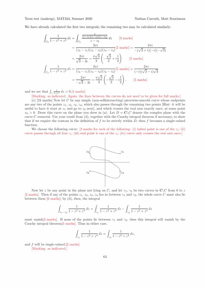
Term test (makeup), MAT334, Summer 2020 Nathan Carruth, Matt Sourisseau
We have already calculated the first two integrals; the remaining two may be calculated similarly:
∫
C3
1
1− z2 + z4dz =
∫
C3
1(z−z1)(z−z2)(z−z4)
z − z3dz [3 marks]
=2πi
(z3 − z1)(z3 − z2)(z3 − z4)[2 marks] =
2πi
−(√3 + i)(−i)(−
√3)
=2πi√3− 3i
=π√3
3
(
−√3
2+ i
1
2
)
[5 marks]
∫
C4
1
1− z2 + z4dz =
2πi
(z4 − z1)(z4 − z2)(z4 − z3)[5 marks] =
2πi
(−i)(√3− i)
√3
=2πi
−√3− 3i
=π√3
3
(
−√3
2− i
1
2
)
, [5 marks]
and we see that∫
γ1
1+z4 dz = 0.[4 marks]
[Marking: as indicated. Again, the lines between the curves do not need to be given for full marks.](e) [24 marks] Now let C be any simple (non-selfintersecting) piecewise-smooth curve whose endpoints
are any two of the points z1, z2, z3, z4, which also passes through the remaining two points [Hint: it will beuseful to have it start at z1 and go to z2 next], and which crosses the real axis exactly once, at some pointx0 > 0. Draw this curve on the plane you drew in (a). Let D = C\C denote the complex plane with thecurve C removed. Use your result from (d), together with the Cauchy integral theorem if necessary, to showthat if we require the contour in the definition of f to be strictly within D, then f becomes a single-valuedfunction.
We choose the following curve: [2 marks for each of the following: (i) initial point is one of the zi; (ii)curve passes through all four zi; (iii) end point is one of the zi; (iv) curve only crosses the real axis once.]
z1z2
z3 z4
Now let z be any point in the plane not lying on C, and let γ1, γ2 be two curves in C\C from 0 to z[2 marks]. Then if any of the points z1, z2, z3, z4 lies in between γ1 and γ2, the whole curve C must also liebetween them [6 marks]; by (d), then, the integral
∫
γ1−γ2
1
1− z2 + z4dz =
∫
γ1
1
1− z2 + z4dz −
∫
γ2
1
1− z2 + z4dz
must vanish[3 marks]. If none of the points lie between γ1 and γ2, then this integral will vanish by theCauchy integral theorem[3 marks]. Thus in either case,
∫
γ1
1
1− z2 + z4dz =
∫
γ2
1
1− z2 + z4dz,
and f will be single-valued.[2 marks][Marking: as indicated.]
63

Term test (makeup), MAT334, Summer 2020 Nathan Carruth, Matt Sourisseau
(f) [16 marks] Using the single-valued version of f described in (e), calculate
limz→x+
0
f(z)− limz→x−
0
f(z),
where z → x±0 means that z approaches from the right (+) or left (−) of the curve C. [Hint: can you seehow to apply your result from (c)?] Does this difference of limits depend on your choice of C? (You do notneed to give a justification.)
[2(a) and 3(f) correspond to Quiz 2.]Since f is single-valued, we may use any two curves γ1, γ2[3 marks]. We use the following curves: [2
marks for each curve; curves should form a closed loop containing only two of the zi – it doesn’t matterwhich two – and not intersecting the curve C except at its intersection with the real axis]
z1z2
z3 z4
γ2
γ1
Now 1/(1− z2 + z4) is continuous at x0, so in the limit
limz→x+
0
f(z)− limz→x−
0
f(z) =
∫
γ2
1
1− z2 + z4dz −
∫
γ1
1
1− z2 + z4dz [2 marks]
= −∫
γ1−γ2
1
1− z2 + z4dz[3 marks] = −π[2 marks]
by (c). It is quite clear that this does not depend on the choice of C, since regardless of the choice of Cthe curve γ1 − γ2 must enclose exactly the two points z1 and z2, which entirely determines the integral of1/(1− z2 + z4) over γ1 − γ2.[2 marks]
[Marking: as indicated.]
64

MAT334, 2020. I, §26 [July 7 – 9] Convergence Nathan Carruth
Summary:• We give an additional formula for the coefficients in a Laurent series expansion, and discuss how todetermine the region of convergence of the series.
• We then discuss poles, essential singularities, and zeros, based on Taylor and Laurent series expansions.• We define residues, and state the residue theorem.
(Goursat, §§40 – 43.)24. Laurent series, revisited. Recall from before the term test that if we have a function f , analytic
between two circles both centred at a, say C and C′, with C′ contained inside C, then if we define
an =1
2πi
∫
C
f(z′)
(z′ − a)n+1dz′ (n ≥ 0), bn =
1
2πi
∫
C′
(z′ − a)n−1f(z′) dz′, (n ≥ 1) (1)
we have the following series expansion for f :
f(z) =
∞∑
n=0
an(z − a)n +
∞∑
n=1
bn1
(z − a)n, (2)
and the series on the right-hand side converge on the annular region between C and C′. Now since f isanalytic between C and C′, as are the quantities (z′ − a)−(n+1) and (z′ − a)n−1 in the definitions of an andbn, the Cauchy integral theorem allows us to evaluate an and bn over any simple closed curve γ which liesentirely in the annular region between C and C′. Suppose that we therefore replace C and C′ in (1) by γ.Then, noting that we may write
bn =1
2πi
∫
γ
f(z′)
(z′ − a)−n+1dz′,
we see that if we define
Jn =
{an, n ≥ 0,b−n, n < 0,
we see that we have for all n ∈ Z, positive and negative,
Jn =1
2πi
∫
γ
f(z′)
(z′ − a)n+1dz′, (3)
and moreover that we may write the series expansion for f given above as
f(z) =∞∑
n=0
Jn(z − a)n +∞∑
n=1
J−n(z − a)−n
=
∞∑
n=0
Jn(z − a)n +
−∞∑
n=−1
Jn(z − a)n =
∞∑
n=−∞Jn(z − a)n, (4)
where this last sum is essentially defined by the expression on the right-hand side of the first line.0
There is no essential difference between the expansions (2) and (4); they are just different ways ofexpressing the same information. On the other hand, the expression (3) is certainly more symmetric andprobably easier to remember than the expression (1). We pay for this in some sense, though, by the fact thatthe expansion (4) in some sense hides the singular terms, and we must keep in mind that if n is negative theterms (z − a)n are singular at z = a.
25. Region of convergence. There are various ways of determining the region of convergence of apower or Laurent series. Perhaps the most elementary way is to apply the root test we learned in elementary
0 Note that this is how we define improper integrals of the form∫ +∞−∞ f(x) dx in elementary calculus: we
pick some point a ∈ R and define the integral to be the sum∫ a
−∞ f(x) dx +∫ +∞a
f(x) dx, much as we may
define this last series as∑−1
n=−∞ Jn(z − a)n +∑∞
n=0 Jn(z − a)n.
65

MAT334, 2020. I, §25 [July 7 – 9] Convergence Nathan Carruth
calculus. Let us first recall the root test for a series of positive real numbers: if cn ≥ 0 for all n, then theseries ∞∑
n=0
cn
will converge if the quantity limn→∞ c1/nn < 1 and diverge if limn→∞ c
1/nn > 1; if limn→∞ c
1/nn = 1 then the
test is indeterminate and we must do something else. Now suppose that we have a Taylor series
∞∑
n=0
an(z − a)n.
This series will converge if it is absolutely convergent, i.e., if the series of absolute values
∞∑
n=0
|an(z − a)n|
converges. If we apply the root test to this series, we see that the series is convergent if
limn→∞
|an(z − a)n|1/n = |z − a| limn→∞
|an|1/n < 1
and divergent if
limn→∞
|an(z − a)n|1/n = |z − a| limn→∞
|an|1/n > 1.
Let us now define the quantity R by
R−1 = limn→∞
|an|1/n ;
if this limit is zero we set R = ∞, while if the limit is infinite we set R = 0. Then from the foregoing we seethat the series will converge if
|z − a| < R
and diverge if|z − a| > R.
(If |z − a| = R, the root test fails and the series may either converge or diverge.)Now suppose that we consider instead the Laurent series
∞∑
n=1
bn(z − a)−n;
by exactly the same logic, if in this case we define R′ by
R′ = limn→∞
|bn|1/n ,
then we see that the series will converge if
|z − a|−1 <1
R′
and diverge if
|z − a|−1 >1
R′ ;
in other words, it will converge if|z − a| > R′
and diverge if|z − a| < R′.
66

MAT334, 2020. I, §25 [July 7 – 9] Convergence Nathan Carruth
(As usual, the test fails when |z − a| = R′, meaning that it tells us nothing about the convergence ordivergence of the series.) This means that, while Taylor series converge on disks, the singular part of aLaurent series converges instead on the exterior of a disk. The full Laurent series, being the sum of a Taylorseries and a singular part, will converge on the intersection of one disk with the exterior of another disk, i.e.,on an annulus (exactly as we might expect!).1
The preceding method will allow us to find the region where any given Taylor or Laurent series converges,assuming that we can calculate the two limits involved. Thus it is useful when the only thing we know isthe series itself. On the other hand, if we know the function f to which the series converges, then there isa much simpler method, as follows. Let us consider Laurent series; the same logic applies to Taylor series(which are, after all, just Laurent series without no singular part, i.e., with singular part equal to 0). Supposethat f is a function which is analytic between the circles C′ and C, centred at a (with C′ inside of C asusual). Then our results with Laurent series show that the Laurent series of f converges to f everywhere onthis annulus. Now if f were analytic on a larger annulus, say between circles C′
1 and C1, also centred at a,then its Laurent series on the annulus between C′
1 and C1 would converge between C′1 and C1; but by the
Cauchy integral theorem (for example, recall that we can define the coefficients using any curve γ lying inthe annular region) the coefficients of this Laurent series would be the same as those of the original Laurentseries. Thus the original Laurent series must also converge on this larger annulus.
If we take this reasoning to its logical conclusion, we see that the Laurent series will converge on thelargest annular region on which f is analytic. To be a bit more careful, recall that we need f to be continuouson the boundary curves C and C′; thus the Laurent series will converge on the largest annular region suchthat f is analytic in the interior and continuous on the boundary. This means that, if we are attempting tofind where the Laurent series for a given function f is convergent, we need only determine the points wheref is not analytic; the Laurent series will then converge on the largest annular region, centred at a, whichdoes not contain any of these points.
(It is worth pointing out that this method does not apply to the case where we are simply given aLaurent series and do not know the function to which it converges. This is because it is in general notpossible to determine the points where a function is not analytic simply by examining its Laurent series.)
Let us give an example.EXAMPLE. Let us define a function f by
f(z) =
∞∑
n=0
zn
(n!)2+
∞∑
n=1
1
n2z−n.
We will find where these series converge, and then discuss how to use the formulas above to determine itsLaurent series. (In a certain sense this second part is quite pointless since a Laurent series is unique, so theseries expansion on the right-hand side is the Laurent expansion of f around 0. But on the other hand itwill give us some practice in the use of the general formulas.) First of all, it can be shown that
limn→∞
(n!)1/n = ∞;
thus alsolimn→∞
[(n!)2]1/n = ∞,
and so the first series must converge on the entire complex plane.Now it can be shown, using L’Hopital’s rule, that
limn→∞
n1/n = 1,
1 Note that it is, in principle, quite possible that this intersection might be empty, i.e., that the disk outsideof which the singular part converges is larger than the disk inside of which the analytic part converges. Inthis case, the series simply does not converge at any point in the complex plane. If we obtained this resultby starting from some specific function, it would indicate that the function was not analytic on any annularregion centred at a. (This does not, incidentally, mean that the function is never analytic, just that theregion on which it is analytic does not contain any annulus around a.)
67

MAT334, 2020. I, §25 [July 7 – 9] Convergence Nathan Carruth
whencelimn→∞
[n2]1/n = 1,
and the quantity R′ above will be 1, meaning that the second series converges when
|z| > 1.
We pause here for a moment to discuss the relation of this last result to our second method for deter-mining the region of convergence of a Laurent series. Let us define
g(z) =
∞∑
n=1
1
n2z−n
wherever this series converges. Since the series diverges for |z| < 1, the function g must have some singularityon the unit circle. Now the series is clearly absolutely convergent on the unit circle itself (since if |z| = 1 theabsolute value of the terms of the series is simply 1/n2, giving a convergent series); thus g does not divergeat any point on the unit circle. Let us look at its derivative. Differentiating term-by-term, we obtain
g′(z) =∞∑
n=1
−z−n−1
n;
thus
zg′(z) =∞∑
n=1
−z−n
n,
sod
dz[zg′(z)] =
∞∑
n=1
z−n−1 = z−2∞∑
n=0
z−n = z−2 1
1− z−1=
1
z2 − z=
1
z(z − 1).
Now this function clearly has a singularity at z = 1, which is on the unit circle. While it is not entirelyclear how to determine the full function g given this rather peculiar differential operator on g, we can saythat if g were analytic at z = 1, then so would be d/dz[zg′(z)]; since this latter quantity, as just noted, isnot analytic at z = 1, g cannot be analytic there either. (Some further study suggests that g in fact has abranch point at z = 1, but we shall not show that here.) This explains why the series cannot converge on alarger annulus.
Proceeding, let us see how to calculate the coefficients in the Laurent series expansion for f using theformula above. (This is very similar to, though more complicated than, the example we did right before thebreak.) We shall use the formula (3) with a = 0, and γ any curve contained in the region |z| > 1:
Jn =1
2πi
∫
γ
f(z′)
z′n+1dz′.
Substituting in the series definition of f , we have
Jn =1
2πi
∫
γ
∞∑
k=0
1
(k!)2z′ k
z′n+1+
∞∑
k=1
1
k21
z′,k+n+1dz′,
so that if we assume we can interchange sum and integral, then we only need to evaluate the integrals
∫
γ
z′k−n−1 dz′,
∫
γ
z′−k−n−1 dz′.
It is sufficient to determine ∫
γ
z′m dz′
68

MAT334, 2020. I, §25 [July 7 – 9] Isolated singularities Nathan Carruth
where m is any integer (positive or negative). Now if m ≥ 0, then the integrand will be analytic everywhereon the plane (as usual, we set z0 = 1 for all z by convention). Now suppose that m ≤ −1, and writen = −m− 1 ≥ 0; then by the general Cauchy integral formula
∫
γ
z′m dz′ =
∫
γ
1
z′ −mdz′ =
∫
γ
1
z′n+1dz′
= 2πidn
dzn[1]|z=0,
which will be 2πi if n = 0 and 0 if n > 0, since the derivative of a constant is 0. Pulling all of this together,then, we see that
∫
γ
z′m dz′ =
{0, m 6= −12πi, m = −1.
(This is a very useful formula to keep in mind, in general.) Applying this to the above formula for Jn, wesee that for n ≥ 0
Jn =1
2πi
∞∑
k=0
1
(k!)2
∫
γ
z′ k−n−1 dz′ +1
2πi
∞∑
k=1
1
k2
∫
γ
z′−k−n−1 dz′
=1
(n!)2,
since the first integral will be nonzero only when k−n− 1 = −1, i.e., k = n, in the which case it equals 2πi,while the second will be nonzero only when −k − n− 1 = −1, i.e., when k = −n; since in the second seriesk ≥ 1, while n ≥ 0, this is impossible. Similarly, when n ≤ −1
Jn =1
2πi
∞∑
k=0
1
(k!)2
∫
γ
z′ k−n−1 dz′ +1
2πi
∞∑
k=1
1
k2
∫
γ
z′−k−n−1 dz′
=1
(−n)2 ,
by the foregoing. Thus we may write
Jn =
{ 1(n!)2 , n ≥ 0,1n2 , n ≤ −1,
which is exactly the coefficients in the original series (as advertised).26. Isolated singularities. We will now apply Laurent series to study the ways in which functions
can fail to be analytic at a single point. More precisely, suppose that a ∈ C, and let f be a function whosedomain contains a. If f is analytic at a, then a is called a regular point of f ; if f is not analytic at a, thena is called a singular point of f . Now suppose that a is a singular point, but that f is analytic everywhereelse near a; i.e., that there is some r > 0 such that f is analytic on the punctured disk
{z | 0 < |z − a| < r},
i.e., f is analytic everywhere on the disk of radius r centred at a, except of course at a itself. In this case ais called an isolated singular point of f . (Note that branch points are not isolated singular points.)
Let us see what we can learn about isolated singular points from Laurent series. Suppose that a is anisolated singular point of a function f , and that f is analytic on the punctured disk
{z | 0 < |z − a| < r}.
Then on any annular region contained in this punctured disk we will have the Laurent series expansion
f =
∞∑
n=0
an(z − a)n +
∞∑
n=1
bn(z − a)−n,
69

MAT334, 2020. I, §26 [July 7 – 9] Isolated singularities Nathan Carruth
where an and bn are given by the formulas (1) above, and moreover do not depend on the particular choiceof annular region; thus we may consider this to be an expansion for f on the entire punctured disk (whichis, strictly speaking, not an annular region in the sense in which we have been using that term). Let usconsider the singular part of this expansion, namely
∞∑
n=1
bn(z − a)−n.
There are three possibilities: (i) bn = 0 for all n; (ii) bn 6= 0 for only finitely many n; (iii) bn 6= 0 for infinitelymany n. In the first case, it can be shown that by defining f(a) = a0, the function f can be made analyticon the whole disk {z | |z − a| < r}, so that the ‘singularity’ is not really a singularity at all; this is called a‘removable singularity’. In the second case we say that the function has a pole at a, while in the third casewe say that it has an essential singularity at a.
Let us give a couple examples.EXAMPLES. 1. Let f = 1/ sin z; then clearly f is analytic everywhere except where sin z = 0, i.e.,
everywhere except for z = nπ, n ∈ Z. Each of these points must therefore be an isolated singularity of f .Let us consider the isolated singularity at z = 0, and see if we can determine the Laurent series for f there.Now we have
sin z =
∞∑
k=0
(−1)k
(2k + 1)!z2k+1 = z
∞∑
k=0
(−1)k
(2k + 1)!z2k.
Now the final series above must converge on the entire complex plane; essentially, this is because it convergesat z = 0, and other than at that point it is equal to a function analytic on the punctured plane {z | z 6= 0}.(If you want to use this fact in your homework solutions, you need to write in a bit more detail!) Let usdenote this function by φ(z), i.e.,
φ(z) =
∞∑
k=0
(−1)k
(2k + 1)!z2k.
Then since φ(0) = 1 6= 0, there must be some disk D around 0 on which φ 6= 0. On this disk, then, 1/φ mustbe analytic, and hence can be expanded as
1
φ(z)=
∞∑
k=0
akzk
for some set of coefficients ak, which we could determine by division of series but won’t. Thus f can bewritten as
f(z) =1
zφ(z)=
1
z
∞∑
k=0
akzk =
a0z
+
∞∑
k=0
ak+1zk.
Thus z = 0 is a pole for f . We say that it is a pole of order 1 ; we shall define this in general momentarily.2. Now let us consider the function f(z) = e1/z. Clearly, f is analytic everywhere except at z = 0, so
that 0 is an isolated singular point of f . Now for any complex number z we have
ez =
∞∑
k=0
1
k!zk;
thus for any nonzero complex number z we must have
e1/z =
∞∑
k=0
1
k!z−k,
and this must therefore be the Laurent expansion for f around 0. Since f has infinitely many nonzerocoefficients in its singular part, 0 must be an essential singularity for f .
70
MAT334, 2020. I, §26 [July 7 – 9] Residues Nathan Carruth
To return to our general treatment, suppose that a is a pole of a function f ; this means that a is anisolated singularity of f , and that the singular part of the Laurent expansion of f around a has finitely manynonzero coefficients. Suppose that m is the largest integer for which bm 6= 0, i.e., that bm 6= 0 while bk = 0for all k > m; then we say that a is a pole of order m of f . This explains our terminology in the first exampleabove.
In other words, a function f has a pole of order m at a if near a
f(z) =
∞∑
n=0
an(z − a)n +b1
z − a+ · · ·+ bm
(z − a)m,
and moreover bm 6= 0.There is a nice relationship between poles and zeros. Recall that a polynomial p = a0 + · · · + anz
n issaid to have a zero of order m at a point a if it is divisible by (z − a)m, i.e., if there is another polynomial qsuch that q(a) 6= 0 and
p(z) = (z − a)mq(z).
Now evidently this same definition can be applied to Taylor series. Specifically, suppose that a function f isanalytic near a point a; then we may expand it in its Taylor series about a as
f(z) =∞∑
n=0
an(z − a)n.
Now f is said to have a zero of order m at a if there is an analytic function φ near a such that φ(a) 6= 0 and
f(z) = (z − a)mφ(z).
In this case, it is easy to see that the first m terms of the Taylor series for f must all vanish, i.e., that wemust have
f(z) = am(z − a)m + am+1(z − a)m+1 + · · · .
Now consider 1/f(z) near z = a; by the foregoing, we have
1
f(z)=
1
(z − a)mφ(z)=
1
φ(z)(z − a)−m;
now since φ(a) 6= 0, as we saw in Example 1 above, φ(z) must be nonzero on some disk centred at a; thus1/φ(z) must be analytic on this disk, say with power series
1
φ(z)=
∞∑
n=0
cn(z − a)n,
and moreover c0 = 1φ(a) 6= 0. Thus
1
f(z)=
1
(z − a)m
∞∑
n=0
cn(z − a)n
=∞∑
n=0
cn+m(z − a)n +cm−1
z − a+ · · ·+ cm
(z − a)m,
which shows that 1/f must have a pole of order m at z = a. This logic works to show the reverse implicationalso, namely that if a function g has a pole of order m at z = a, then 1/g must have a zero of order m atz = a. Thus, in some sense, poles and zeroes are complementary to each other.
71

MAT334, 2020. I, §26 [July 7 – 9] Residues Nathan Carruth
27. Residues. Suppose that a is an isolated singular point of the function f , and let γ be a simpleclosed curve in the punctured disk about a on which f is analytic, and which moreover encloses the point a.Then we may write the Laurent series for f about a,
f(z) =∞∑
n=0
an(z − a)n +∞∑
n=1
bn(z − a)−n.
Thus, assuming that we can interchange sum and integral, we have
∫
γ
f(z′) dz′ =∞∑
n=0
an
∫
γ
(z′ − a)n dz′ +∞∑
n=1
bn
∫
γ
(z′ − a)−n dz′;
by the same logic we used in the examples in the previous section, all of these integrals will vanish exceptfor the one with the power (z′ − a)−1, and that one will give 2πi. Thus we have
∫
γ
f(z′) dz′ = 2πib1.
The quantity b1, which is the coefficient of the (z′ − a)−1 term in the Laurent expansion of f about z = a,is called the residue of f at the point a.
At present, this logic might seem slightly circular, since the equation above is actually equivalent to thedefinition of b1 given above. If we had no other way to find Laurent series than through the definitions ofan and bn in terms of integrals, then this would indeed be circular. However, as our examples above havehopefully suggested, there are ways of computing Laurent series that do not involve calculating integrals atall. This means that there are other methods of computing residues. These methods allow us to apply theformula above in meaningful ways.
We may generalise this result as follows to obtain an even more useful one. Suppose that we begin witha curve γ, and that f is analytic everywhere inside γ except at certain isolated singular points z1, · · ·, zn.Let βj denote the residue of f around zj , for j = 1, · · · , n. Then it follows from the generalised Cauchytheorem that we may write
∫
γ
f(z′) dz′ = 2πin∑
j=1
βj .
This result, known as the residue theorem, is extremely useful in the applications we shall make of contourintegrals to evaluating definite integrals on the real line.
72
MAT334, 2020. , §27 [2020/10/7] Nathan Carruth
MAT334, COMPLEX VARIABLES, SUMMER 2020. PROBLEMS FOR JULY 6 – 10
Due Tuesday, July 14, at 3:30 PM EDT.
1. Using the formulas in Goursat, §§35, 37, find the Laurent series for
f(z) =sin z
z
around z = 0. How does this series compare to the Taylor series for sin z around z = 0? On what set doesit converge? Justify your answer.
Let us write
f(z) =
∞∑
n=0
an(z − a)n +
∞∑
n=1
bn(z − a)−n,
and let γ be a circle around z = 0; then we have the formulas
an =1
2πi
∫
γ
f(z′)
(z′ − 0)n+1dz′
bn =1
2πi
∫
γ
f(z′)(z′ − 0)n−1 dz′.
Substituting in f(z) = (sin z)/z, the first of these gives
an =1
2πi
∫
γ
sin z′
z′n+2dz′[1 mark]
=1
2πi· 2πi
(n+ 1)!
dn+1
dzn+1sin z
∣∣∣∣z=0
=1
(n+ 1)!
dn+1
dzn+1sin z
∣∣∣∣z=0
; [2 marks]
thus a0 = 1, a1 = 0, a2 = −1/6, a3 = 0, etc., and in general a2k+1 = 0 while a2k = (−1)k/(2k+ 1)![1 mark].Now
b1 =1
2πi
∫
γ
sin z′
z′dz′[1 mark] =
1
2πisin 0 = 0, [1 mark]
while if n > 1
bn =1
2πi
∫
γ
sin z′(z′ − 0)n−2 dz′ = 0[1 mark]
by the Cauchy integral theorem, since the integrand is analytic everywhere. Thus we have
sin z
z=
∞∑
k=0
(−1)k
(2k + 1)!z2k.[1 mark]
Now recall that the Taylor series for sin z is
sin z =
∞∑
k=0
(−1)k
(2k + 1)!z2k+1;
in other words, the Laurent series for (sin z)/z is just the Taylor series for sin z, divided term-by-term by z,as we might expect[1 mark]. Since the Taylor series for sin z converges everywhere on the complex plane,the Laurent series above will converge to an analytic function everywhere except possibly at z = 0; but atz = 0 the series also clearly converges to 1, so the series converges on the entire complex plane.[1 mark]
2. Again using the formulas in Goursat, §§35, 37, find the Laurent series for
f(z) =ez
(z − 2)2
73

MAT334, 2020. , §27 [2020/10/7] Nathan Carruth
around z = 2. How does this compare to the Taylor series for ez around z = 2? [Hint: recall that ea+b = eaeb;can you use this to find the Taylor series?] On what set does this Laurent series converge? Again, justifyyour answer.
We use the same formulas as in question 1. Thus we have, first of all, letting now γ denote a circlearound z = 2,
an =1
2πi
∫
γ
f(z′)
(z′ − 2)n+1dz′
=1
2πi
∫
γ
ez′
(z′ − 2)n+3dz′[1 mark] =
1
(n+ 3)!
dn+2
dzn+2ez∣∣∣∣z=2
[2 marks] =e2
(n+ 2)!, [1 mark]
by the Cauchy integral formula for derivatives, while
b1 =1
2πi
∫
γ
f(z′) dz′[1 mark] =1
2πi
∫
γ
ez′
(z′ − 2)2dz′ = e2, [1 mark]
b2 =1
2πi
∫
γ
f(z′)(z′ − 2) dz′ =1
2πi
∫
γ
ez′
z′ − 2dz′ = e2, [1 mark]
while for n > 2
bn =1
2πi
∫
γ
f(z′)(z′ − 2)n−1 dz′ =1
2πi
∫
γ
ez′
(z′ − 2)n−3 dz′ = 0[1 mark]
by the Cauchy integral theorem. Thus we have the expansion
f(z) =e2
(z − 2)2+
e2
z − 2+
∞∑
n=0
e2
(n+ 2)!(z − 2)n.[2 marks]
Now the Taylor series for ez around z = 2 can be found as follows:
ez = e2ez−2 = e2∞∑
n=0
1
n!(z − 2)n =
∞∑
n=0
e2
n!(z − 2)n; [2 marks]
from this we see that the above series is simply this series, divided by (z − 2)2 term-by-term, as we wouldexpect.[1 mark]
Now the Taylor series for ez around z = 2 converges on the entire complex plane; thus the series abovefor f will converge everywhere where it is defined, i.e., on the punctured plane {z ∈ C | z 6= 2}.[2 marks]
74

MAT334, 2020. I, §27 [July 14 – 16] Evaluation of integrals Nathan Carruth
Summary:• We give examples of applications of the residue theorem to the evaluation of definite integrals on thereal axis.
• We then give theorems for showing that integrals over semicircles go to zero, and provide additionalmethods for computing residues.
(Goursat, §§44 – 46.)28. Evaluation of definite integrals. Recall the residue theorem from last time: if f is a function
which is continuous on a simple closed curve γ, and analytic inside γ except potentially at a finite numberof isolated singularities z1, · · ·, zn, at which it has residues β1, · · ·, βn, respectively. Then we have
∫
γ
f(z′) dz′ = 2πi
n∑
j=1
βj .
Let us see by way of an example – which could also be done by elementary methods – how this result canbe applied to evaluate definite integrals.
EXAMPLE. Consider the integral∫ +∞
−∞
1
1 + x2dx.
Since this integral converges, it is equal to the limit
limR→+∞
∫ R
−R
1
1 + x2dx;
since arctanx is an antiderivative of 1/(1+x2), by the fundamental theorem of calculus this integral is equalto
limR→+∞
(arctanR− arctan(−R)) = π
2−(
−π2
)
= π.
Now suppose that we consider∫ R
−R1
1+x2 dx as a contour integral in the complex plane, with the contourtaken along the real axis; then we get the following picture.
x
y
−R RLR
As it stands this does not seem to have gotten us anywhere. Note though that the integrand here isanalytic on the entire plane except for (simple) poles at ±i. Thus if it were possible to somehow augmentthe contour LR in order to obtain a closed curve (we speak of closing the contour), we would be able toapply either the Cauchy integral theorem – if the closed curve did not contain either of the poles – or theresidue theorem – otherwise – in order to evaluate the integral over the full closed contour. If, additionally,it were possible somehow to compute the integral over the additional contour, at least in the limit of largeR, we would then be able to compute our original integral.
In general there are multiple ways of closing the contour; i.e., there are multiple different possible choicesfor the additional curve to be used to produce a closed contour from the original one. Consider the semicircleCR in the upper half-plane as in the following picture.
x
y
−R RLR
CR
i
75

MAT334, 2020. I, §28 [July 14 – 16] When∫
CRf(z) dz → 0 Nathan Carruth
Remember that our technique will only be useful if we have a way of computing∫
CR1/(1 + z2) dz; we
claim that in fact
limR→∞
∫
CR
1
1 + z2dz = 0.
In class we showed this by parameterising the curve CR and considering the resulting integrand; here we usea slightly simpler method. Recall that, if f is continuous on a simple closed curve γ, with maximum M onγ, then ∣
∣∣∣
∫
γ
f(z) dz
∣∣∣∣≤M |γ|,
where |γ| is the length of the curve γ. Now clearly |CR| = πR (since CR is a semicircle of radius R); further,if z is any point on CR then we may write z = Reit for some t ∈ [0, π], and thus
∣∣∣∣
1
1 + z2
∣∣∣∣=
∣∣∣∣
1
1 +R2e2it
∣∣∣∣=
∣∣∣∣
R−2
e2it +R−2
∣∣∣∣= R−2
∣∣e2it +R−2
∣∣−1.
Now by the triangle inequality we may write
∣∣e2it +R−2
∣∣ ≥
∣∣e2it
∣∣−∣∣R−2
∣∣ = 1−R−2,
so that when we take the limit R → ∞ we have
R−2∣∣e2it +R−2
∣∣−1 ≤ R−2(1−R−2)−1 ≤ 1
R2 − 1,
which goes to zero. Thus
limR→∞
∫
CR
1
1 + z2dz = 0
as claimed.Now for any R > 1, the closed curve LR + CR will enclose the single pole at i. Let us calculate the
residue of 1/(1 + z2) at z = i. We have
1
1 + z2=
1
(z − i)(z + i)=
1/(z + i)
z − i;
if we think of expanding 1/(z + i) as
1
z + i=
∞∑
n=0
cn(z − i)n
(which we can do since 1/(z + i) is analytic near i), then
1
1 + z2=c0 + c1(z − i) + c2(z − i)2 + · · ·
z − i=
c0z − i
+ c1 + c2(z − i) + · · · ,
and the residue of 1/(1 + z2) is clearly c0. But c0 = 1/(z + i)|z=i = 1/(2i). Thus at the end of the day wehave for all R > 1 ∫
LR
1
1 + z2dz +
∫
CR
1
1 + z2dz = 2πi · 1
2i= π;
and in the limit R → ∞, the integral over LR goes to∫ +∞−∞ 1/(1 + x2) dx while the integral over CR goes to
zero. Thus at the end of the day∫ +∞
−∞
1
1 + x2dx = π,
exactly as we found above.There are two key points in the above procedure: (i) we have to find a curve CR (which need not be a
semicircle, in general, or any segment of a circular path) which will close the contour LR, and over which
76

MAT334, 2020. I, §28 [July 14 – 16] When∫
CRf(z) dz → 0 Nathan Carruth
we can integrate f ; (ii) we have to evaluate the residues of f at its singularities inside the closed contourLR +CR. We shall now give methods for addressing these two points: first, by providing general conditionsunder which integrals along circular arcs like CR go to zero as R → ∞; second, by providing additionalmethods for calculating residues.
29. When∫
CRf(z) dz → 0. First we have the following fairly straightforward generalisation of the
example from the previous section. Suppose that f is a function analytic on the exterior of a circle of radiusR for a suitably large R (in other words, if f has any singularities they are not too far from the origin).Suppose that for suitably large R there is a number MR such that for all z ∈ CR we have |f(z)| < MR, andthat limR→∞RMR = 0. Then
limR→∞
∫
CR
f(z) dz = 0.
To see this, note that the length of CR is πR; thus
∣∣∣∣
∫
CR
f(z) dz
∣∣∣∣≤ πRMR,
and as this latter quantity goes to zero by assumption, the integral must also, by the squeeze theorem.We may apply this to the example in the previous section as follows. Suppose that z ∈ CR. Then we
have
|f(z)| =∣∣∣∣
1
1 + z2
∣∣∣∣≥ 1
|z2| − 1=
1
R2 − 1,
where we have used the triangle inequality as before; since R/(R2 − 1) → 0 as R → ∞, the above resultshows that limR→∞
∫
CRf(z) dz = 0 as well.
We note in passing that it is actually sufficient to show that if z → ∞ along circles CR, then we musthave limz→∞ zf(z) = 0. More precisely, what this means is that zf(z) can be made arbitrarily small bytaking z ∈ CR with |z| = R arbitrarily large. In cases like the foregoing this is easier to apply, since we have
limz→∞
z
1 + z2= lim
z→∞z−1
1 + z−2,
and since the numerator goes to 0 while the denominator goes to 1, the fraction must go to zero. To befully rigorous, though, we would have to explain how this kind of a limit – restricting z to lie on a particularfamily of curves – relates to usual limits, but we shall not do that here. This method can also be used toshow easily what we saw in class: suppose that
f(z) =P (z)
Q(z),
where P and Q are polynomials, and degQ ≥ degP + 2. Then we can write
limz→∞
zf(z) = limz→∞
z(a0 + · · ·+ anzn)
b0 + · · ·+ bn+2zn+2,
where bn+2 6= 0 but we may have an = 0. By dividing numerator and denominator by zn+2, this becomes
limz→∞
anz−1 + an−1z
−2 + · · ·+ a0z−n−1
bn+2 + bn+1z−1 + · · ·+ b0z−n−2= 0,
since the numerator goes to 0 while the denominator goes to bn+2 6= 0.Let us do an example.EXAMPLE. Compute
∫ +∞
−∞
cosx
1 + x2dx.
77

MAT334, 2020. I, §29 [July 14 – 16] When∫
CRf(z) dz → 0 Nathan Carruth
We note first that the integrand has poles in the complex plane at ±i, just like the example above. Let usnow consider what kind of contour we can use to close the line LR. Now we have
cos z =1
2
(eiz + e−iz
).
Now suppose that z = a+ ib; then
cos z =1
2
(eia−b + e−ia+b
),
and we see that the first term goes to zero on the upper half-plane (b > 0) while the second term goes toinfinity exponentially there, and vice versa on the lower half-plane. (We ignore for the moment what happenson the real axis when b = 0.) Thus it does not seem that there is any way of closing the contour so as tohave
∫
CRf(z) dz = 0 as regardless of whether CR is in the upper or lower half-plane the integrand will have
one term going to infinity.There are two ways of dealing with this. The more general one is to split the original integral up into
two pieces,∫ +∞
−∞
eix
2(1 + x2)dx,
∫ +∞
−∞
e−ix
2(1 + x2)dx,
and then closing these two integrals in the upper and lower half-plane, respectively; for example, using inturn the curves CR and C′
R in the following figure. We shall see similar cases to this in the future. For nowwe use a simpler method. Note that we have also
cos z = Re eiz ,
x
y
−R RLR
CR
C ′
R
i−i
so since we are integrating along the real axis, we may write
∫ +∞
−∞
cosx
1 + x2dx =
∫ +∞
−∞
Re eix
1 + x2dx = Re
∫ +∞
−∞
eix
1 + x2dx.
We try closing this integral in the upper half-plane as described above; thus let CR denote a semicircle fromR to −R in the upper half-plane, as indicated in the above figure. If z = a+ ib ∈ CR, then b ≥ 0, so we have
∣∣eiz∣∣ =
∣∣eiae−b
∣∣ = e−b ≤ 1,
and ∣∣∣∣
eiz
1 + z2
∣∣∣∣≤ 1
|1 + z2| ≤1
R2 − 1
as before, and since limR→∞R/(R2 − 1) = 0 we have
limR→∞
∫
CR
eiz
1 + z2dz = 0.
78

MAT334, 2020. I, §29 [July 14 – 16] Computing residues Nathan Carruth
Thus we need only calculate the residues of eiz/(1+z2) in the upper half-plane. Now in the upper half-planethis function is singular only at z = i; if we proceed in the same way we did in the previous example (weshall give a general method for this right after this example), we see that the residue is
ei·i
2i=
1
2ei,
and finally by the residue theorem and the fact that∫
CR
eiz
1+z2 dz → 0 as R → ∞, that our original integralis ∫ +∞
−∞
eiz
1 + z2dz = 2πi · 1
2ei=π
e.
This is already real, so that we have∫ +∞
−∞
cosx
1 + x2dx =
π
e.
30. Methods for computing residues. In the previous two examples we have tacitly applied thefollowing result:
Suppose that f(z) has a simple pole at z = a. Then
Resaf(z) = limz→a
(z − a)f(z).
This is quite simple to see. Since f has a simple pole, there must be a function φ(z) which is analytic andnonzero at a such that
f(z) =φ(z)
z − a.
Then, proceeding as in the two examples above, it is easy to see that Resaf(z) = φ(a); alternatively, we mayuse the Cauchy integral formula (here γ is a small circle around a such that f is analytic on and within γ):
Resaf(z) =1
2πi
∫
γ
f(z) dz =1
2πi
∫
γ
φ(z)
z − adz = φ(a).
Butφ(a) = lim
z→aφ(z) = lim
z→a(z − a)f(z),
which establishes our result.We may extend the above result to poles of higher order. Suppose that f has instead a pole of order m
at z = a. Then we may write
f(z) =φ(z)
(z − a)m,
where as before φ is analytic and nonzero at a; thus (letting as before γ denote a small circle around a withinand on which f is analytic)
Resaf(z) =1
2πi
∫
γ
φ(z)
(z − a)mdz =
1
(m− 1)!
dm−1
dzm−1φ(z)
∣∣∣∣z=a
=1
(m− 1)!limz→a
dm−1
dzm−1(z − a)mf(z).
In other words, to calculate the residue of a function f at a pole of order m, we first multiply f by (z− a)m,differentiate m− 1 times, evaluate at a, and divide by (m − 1)!. (Note that m ≥ 1, so that m − 1 ≥ 0 andthe foregoing makes sense.) Note that this formula reduces to the previous one in the case m = 1. Note alsothat to apply it we must first determine the order of the pole a.
In the case that f(z) = P (z)/Q(z), as before, where P and Q have no common factors and Q has norepeated roots, we see that every pole of f will be simple, and the residue at a pole z0 will be
limz→z0
(z − z0)f(z) = limz→z0
P (z)
Q(z)/(z − z0)=
P (z0)
Q′(z0),
79

MAT334, 2020. I, §30 [July 14 – 16] Computing residues Nathan Carruth
since Q(z0) = 0 (as z0 is a pole of f and therefore must be a zero of Q) and this allows us to write
limz→z0
Q(z)
z − z0= lim
z→0
Q(z)−Q(z0)
z − z0= Q′(z0).
Q′(z0) 6= 0 since by assumption the roots of Q are not repeated.Let us give an example.EXAMPLES. 1. Evaluate the integral
∫ +∞
−∞
1
(1 + x2)2dx.
We note that the integrand, extended to the complex plane, has poles at ±i, each of order 2. We expectthat we can close the contour using a half-circle CR from R to −R in the upper half-plane, as we have donein the other examples above (see the picture). To see that we can in fact do this, we apply the result fromthe previous section: for z ∈ CR, we have
|1 + z2| ≥ R2 − 1, |1 + z2|2 ≥ (R2 − 1)2,
∣∣∣∣
1
(1 + z2)2
∣∣∣∣≤ 1
(R2 − 1)2,
x
y
−R RLR
CR
i
and since R/(R2 − 1)2 clearly goes to zero as R → ∞, we have
limR→∞
∫
CR
1
(1 + z2)2dz = 0.
Thus we need only calculate the residue of 1/(1 + z2)2 at i. Since i is a pole of order 2 of 1/(1 + z2)2, thiswill be, since (1 + z2)2 = (z − i)2(z + i)2,
1
(2− 1)!limz→i
d2−1
dz2−1(z − i)2 · 1
(1 + z2)2=
d
dz
1
(z + i)2
∣∣∣∣z=i
= − 2
(z + i)3
∣∣∣∣z=i
= − 2
−8i= −1
4i,
and the integral will be∫ +∞
−∞
1
(1 + x2)2dx = 2πi ·
(
−1
4i
)
=π
2.
(It is worth pointing out here that it is always a good idea to make sure that our final answer makes sense:for example, here we are integrating a real-valued function, so we expect to get a real number as the result;and it is in fact a positive real-valued function, so we expect to get a positive real number as the result, aswe have. Had we gotten a negative real number, or a complex number with a nonzero imaginary part, itwould mean we had made a mistake somewhere earlier which we would need to go back and fix.)
2. Let us evaluate the integral∫ +∞
−∞
eikx
(1 + x2)2dx.
Here we clearly have the same kind of issue that we had in our example in section 29 above; namely,whether we close the contour in the upper or the lower half-plane will depend on the sign of k. Let us firstsuppose that k ≥ 0. Then if z = a+ ib is in the upper half-plane, so that b ≥ 0, then as in the example justcited we have
eikz = e−kbeika,
80

MAT334, 2020. I, §30 [July 14 – 16] Computing residues Nathan Carruth
which is bounded in absolute value by e−kb ≤ 1; in other words, the integrand here on the semicircle CR inthe next figure will be bounded by the same quantity as we had for 1/(1+ z2)2 in the previous example, andthe integral over CR will go to zero as R → ∞ as there. More carefully, recall that we just showed that onCR ∣
∣∣∣
1
(1 + z2)2
∣∣∣∣≤ 1
(R2 − 1)2;
x
y
−R RLR
CR
C ′
R
i−i
thus when k ≥ 0 and z ∈ CR (so that z is in the upper half-plane)
∣∣∣∣
eikz
(1 + z2)2
∣∣∣∣≤ 1
(R2 − 1)2
as well, and since R/(R2 − 1)2 → 0 as R → ∞, we have
limR→∞
∫
CR
eikz
(1 + z2)2dz = 0
by our general results above. Thus it suffices to calculate the residue of eikz/(1 + z2)2 at the pole i, andsince this is still a pole of order 2, its residue is
1
(2− 1)!limz→i
d2−1
dz2−1(z − i)2 · eikz
(1 + z2)2=
d
dz
eikz
(z + i)2
∣∣∣∣z=i
=ikeikz
(z + i)2
∣∣∣∣z=i
− 2eikz
(z + i)3
∣∣∣∣z=i
=ike−k
−4− 2
e−k
−8i= −ie−k
(1
4+
1
4k
)
,
so that the integral for k ≥ 0 is
∫ +∞
−∞
eikx
(1 + x2)2dx = 2πi · (−i)e−k
(1
4+
1
4k
)
=π
2e−k (k + 1) .
Now suppose that k ≤ 0, and consider the curve C′R in the above figure. If z = a+ bi ∈ C′
R, then b ≤ 0, so
eikz = e−kbeika
will still be bounded by 1 in absolute value since k ≤ 0 and b ≤ 0 implies that kb ≥ 0, i.e., −kb ≤ 0. Theexact same logic used above now shows that
limR→∞
∫
C′R
eikz
(1 + z2)2dz = 0,
and we are left with calculating the residue at −i. This is very similar to calculating the residue at i; it isequal to
d
dz
eikz
(z − i)2
∣∣∣∣z=−i
=ikeikz
(z − i)2
∣∣∣∣z=−i
− 2eikz
(z − i)3
∣∣∣∣z=−i
=ikek
−4− 2
ek
8i= iek
(1
4− 1
4k
)
.
81

MAT334, 2020. I, §30 [July 14 – 16] Computing residues Nathan Carruth
Before we can determine the value of the integral, though, there is one additional wrinkle we have not yetmentioned: note that the curve LR +CR was oriented counterclockwise, as required by the Cauchy integralformula; but LR + C′
R is oriented clockwise, which means that we must put in an extra minus sign whenapplying the Cauchy integral formula. More carefully, we have
∫
LR
eikz
(1 + z2)2dz +
∫
C′R
eikz
(1 + z2)2dz = −2πiRes−i
eikz
(1 + z2)2;
thus, finally, our integral is
∫ +∞
−∞
eikx
(1 + x2)2dx = −2πi ·
[
iek(1
4− 1
4k
)]
=π
2ek (1− k) .
Pulling all of this together, then, we have finally that
∫ +∞
−∞
eikx
(1 + x2)2dx =
π
2e−|k|(1 + |k|),
since |k| = k when k ≥ 0 and |k| = −k when k ≤ 0.For those who know something about Fourier transforms, it is interesting to note the following about the
differentiability of this function. If we expand the exponential out in a Taylor series, we see that (droppingthe π/2 coefficient for convenience)
e−|k|(1 + |k|) =(
1− |k|+ 1
2|k|2 − 1
6|k|3 + · · ·
)
(1 + |k|)
= 1− |k|2 + 1
2|k|2 + 1
2|k|3 − 1
6|k|3 + · · · .
Now a little thought should convince you that |k|n has n derivatives everywhere and n + 1 derivativeseverywhere except 0, where the n + 1th derivative is discontinuous. This shows that e−|k|(1 + |k|) has 3continuous derivatives, which agrees nicely with the fact that the function 1/(1 + x2)2 has 3 moments in L2
(i.e., that the integral of the square of xn/(1 + x2)2 over all of R1 will be finite for n ≤ 3).
82

MAT334, 2020. , §30 [2020/10/7] Nathan Carruth
MAT334, COMPLEX VARIABLES, SUMMER 2020. PROBLEMS FOR JULY 13 – 17
Due Wednesday, July 22, at 3:30 PM EDT.
1. [20 marks] Evaluate the following integrals:
∫ +∞
−∞
1
1 + x4dx,
∫ +∞
−∞
1
1− x2 + x4dx.
(You may cite the term test solutions on the course website in your solution, if you wish.)To evaluate the first integral, we proceed as follows. Let f(z) = 1/(1+ z4), let R > 1, let LR denote the
line segment from −R to R along the real axis, and let CR denote the semicircle of radius R centred at 0 inthe upper half-plane. Then the only poles of f inside the closed contour LR + CR are at (see the picture)
z1 =1√2+ i
1√2, z2 = − 1√
2+ i
1√2,
−R RLR
CR
z1z2
so that we may write, by the residue theorem,
∫
LR
1
1 + z4dz +
∫
CR
1
1 + z4dz = 2πi
[
Resz11
1 + z4+Resz2
1
1 + z4
]
.
Moreover, if z = Reit, t ∈ [0, π] is some point in CR, then we have
R|f(z)| = R
∣∣∣∣
1
1 +R4e4it
∣∣∣∣≤ R
R4 − 1=
R−3
1−R−4,
which clearly goes to zero as R→ ∞. Thus we have
limR→∞
∫
CR
1
1 + z4dz = 0
as well, and therefore our original integral is
∫ +∞
−∞
1
1 + x4dx = lim
R→∞
∫
LR
1
1 + z4dz = 2πi
[
Resz11
1 + z4+Resz2
1
1 + z4
]
=π√2,
where the final answer follows from question 3(c) on the main sitting of the term test.To evaluate the second integral, we proceed in an analogous fashion. Let f(z) = 1/(1 − z2 + z4), let
R > 1, let LR denote the line segment from −R to R along the real axis, and let CR denote the semicircle ofradius R centred at 0 in the upper half-plane. Then the only poles of f inside the closed contour LR + CR
are at (see the picture)
z1 =
√3
2+ i
1
2, z2 = −
√3
2+ i
1
2,
83

MAT334, 2020. , §30 [2020/10/7] Nathan Carruth
−R RLR
CR
z1z2
so that we may write, by the residue theorem,
∫
LR
1
1− z2 + z4dz +
∫
CR
1
1− z2 + z4dz = 2πi
[
Resz11
1− z2 + z4+Resz2
1
1− z2 + z4
]
.
Moreover, if z = Reit, t ∈ [0, π] is some point in CR, then we have
R|f(z)| = R
∣∣∣∣
1
1−R2e2it +R4e4it
∣∣∣∣≤ R
R4 −R2 − 1=
R−3
1−R−2 −R−4,
which clearly goes to zero as R→ ∞. Thus we have
limR→∞
∫
CR
1
1− z2 + z4dz = 0
as well, and therefore our original integral is
∫ +∞
−∞
1
1− x2 + x4dx = lim
R→∞
∫
LR
1
1− z2 + z4dz = 2πi
[
Resz11
1− z2 + z4+Resz2
1
1− z2 + z4
]
= π
where the final answer follows from question 3(c) on the makeup sitting of the term test.
[Marking: for each integral, 2 marks for the setup (description or picture of LR, CR, and the poles); 2marks for the residue theorem (or the Cauchy integral theorem, to relate it to the integral on the term test);3 marks for showing that the integral over CR goes to zero; 3 marks for deducing the final value.]
2. [30 marks] Evaluate the following integrals:
∫ +∞
−∞
sinmx
x(x2 + a2)dx, m, a real, a 6= 0.
∫ +∞
−∞
eikx
1 + x4dx, k any real number. [Hint: Apply your work from problem 1.]
As mentioned in the announcement of July 21, for the first integral all that is required is to set thingsup and then evaluate the residue, ignoring the singularity at z = 0. We thus let LR be the line segmentfrom −R to R, and CR the semicircle centred at 0 with radius R in the upper half-plane; then we see thatthe only singularity the integrand has inside the closed curve LR + CR is at z = ia (where we assume thata > 0 without loss of generality). (See the picture.) Now by the residue theorem we have
∫
LR
sinmz
z(z2 + a2)dz +
∫
CR
sinmz
z(z2 + a2)dz = 2πiResia
sinmz
z(z2 + a2).
84

MAT334, 2020. , §30 [2020/10/7] Nathan Carruth
−R RLR
CR
ia
We leave the issue of how to deal with the integral over CR for later and simply show how to calculate theresidue. Since z2 + a2 = (z − ia)(z + ia), we see that z = ia is a simple pole of (sinmz)/[z(z2 + a2)], andthus the residue may be calculated as follows:
Resiasinmz
z(z2 + a2)= lim
z→ia(z − ia)
sinmz
z(z2 + a2)= lim
z→ia
sinmz
z(z + ia)
= − sinmia
2a2= − i sinhma
2a2,
whence we see that
2πiResiasinmz
z(z2 + a2)=π sinhma
a2.
[Marking: again, 2 marks for the setup, 2 marks for the residue theorem; then 3 marks for computing theresidue.]
Finally, for the last integral we must consider two separate cases depending on whether k > 0 or k < 0.(For k = 0 this is simply the integral from question 1.) Suppose that k > 0, and let LR denote the linesegment from −R to R and CR the semicircle centred at 0 with radius R in the upper half-plane, as usual;then for R > 1 the only poles will be those at
z1 =1√2+ i
1√2, z2 = − 1√
2+ i
1√2,
as found in question 1 (see the picture), and by the residue theorem we have as usual
∫
LR
eikz
1 + z4dz +
∫
CR
eikz
1 + z4dz = 2πi
[
Resz1eikz
1 + z4+Resz2
eikz
1 + z4
]
.
−R RLR
CR
z1z2
Now note that for R > 1 we have, for any z = Reit on CR,∣∣∣∣
1
1 + z4
∣∣∣∣=
∣∣∣∣
1
1 +R4e4it
∣∣∣∣≤ 1
R4 − 1,
85
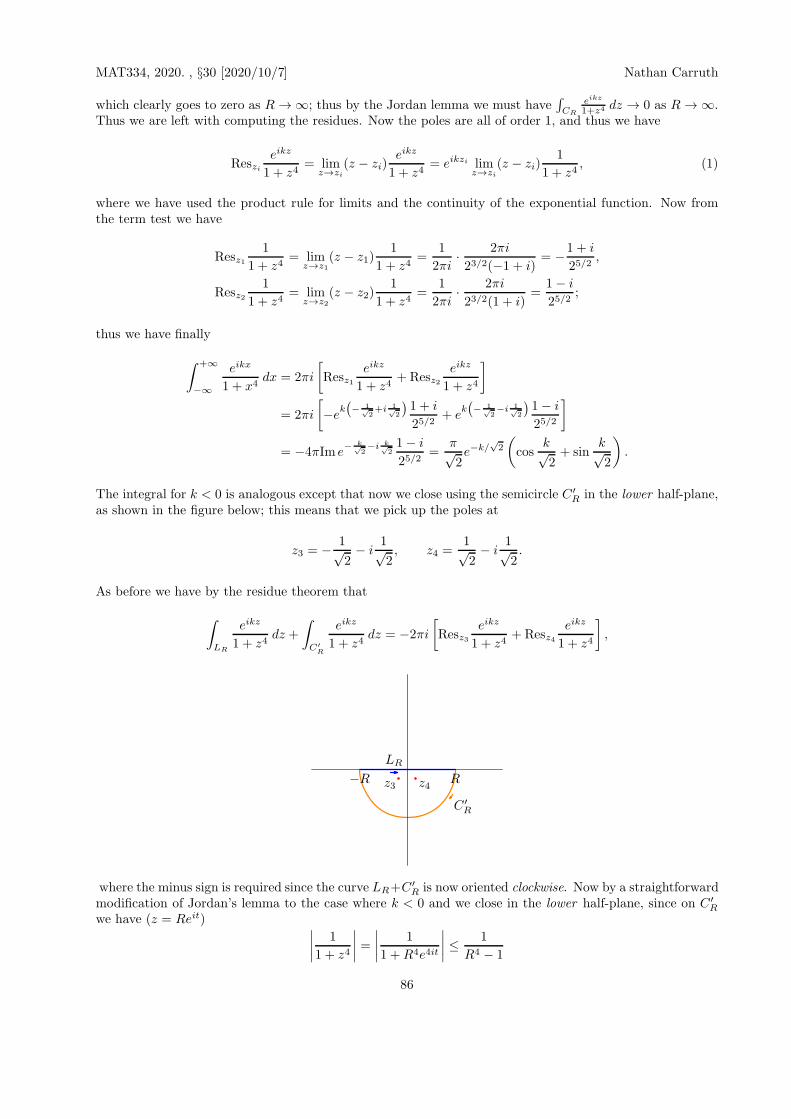
MAT334, 2020. , §30 [2020/10/7] Nathan Carruth
which clearly goes to zero as R → ∞; thus by the Jordan lemma we must have∫
CR
eikz
1+z4 dz → 0 as R → ∞.Thus we are left with computing the residues. Now the poles are all of order 1, and thus we have
Reszieikz
1 + z4= lim
z→zi(z − zi)
eikz
1 + z4= eikzi lim
z→zi(z − zi)
1
1 + z4, (1)
where we have used the product rule for limits and the continuity of the exponential function. Now fromthe term test we have
Resz11
1 + z4= lim
z→z1(z − z1)
1
1 + z4=
1
2πi· 2πi
23/2(−1 + i)= −1 + i
25/2,
Resz21
1 + z4= lim
z→z2(z − z2)
1
1 + z4=
1
2πi· 2πi
23/2(1 + i)=
1− i
25/2;
thus we have finally
∫ +∞
−∞
eikx
1 + x4dx = 2πi
[
Resz1eikz
1 + z4+Resz2
eikz
1 + z4
]
= 2πi
[
−ek(− 1√
2+i 1√
2
)1 + i
25/2+ e
k(− 1√
2−i 1√
2
)1− i
25/2
]
= −4πIm e− k√
2−i k√
21− i
25/2=
π√2e−k/
√2
(
cosk√2+ sin
k√2
)
.
The integral for k < 0 is analogous except that now we close using the semicircle C′R in the lower half-plane,
as shown in the figure below; this means that we pick up the poles at
z3 = − 1√2− i
1√2, z4 =
1√2− i
1√2.
As before we have by the residue theorem that
∫
LR
eikz
1 + z4dz +
∫
C′R
eikz
1 + z4dz = −2πi
[
Resz3eikz
1 + z4+Resz4
eikz
1 + z4
]
,
−R R
LR
C ′
R
z4z3
where the minus sign is required since the curve LR+C′R is now oriented clockwise. Now by a straightforward
modification of Jordan’s lemma to the case where k < 0 and we close in the lower half-plane, since on C′R
we have (z = Reit)∣∣∣∣
1
1 + z4
∣∣∣∣=
∣∣∣∣
1
1 +R4e4it
∣∣∣∣≤ 1
R4 − 1
86

MAT334, 2020. , §30 [2020/10/7] Nathan Carruth
as before, we have that∫
C′R
eikz
1+z4 dz → 0 as R → ∞. Now formula (1) holds just as well for i = 3, 4 as for
i = 1, 2; since from the term test we have
Resz31
1 + z4= lim
z→z3(z − z3)
1
1 + z4=
1
2πi· 2πi
23/2(1− i)=
1 + i
25/2,
Resz41
1 + z4= lim
z→z4(z − z4)
1
1 + z4=
1
2πi· 2πi
23/2(−1− i)=
−1 + i
25/2,
we have finally in this case
∫ +∞
−∞
eikx
1 + x4dx = −2πi
[
Resz3eikz
1 + z4+Resz4
eikz
1 + z4
]
= −2πi
[
ek(
1√2−i 1√
2
)1 + i
25/2− e
k(
1√2+i 1√
2
)1− i
25/2
]
= 4πIm ek√2−i k√
21 + i
25/2=
π√2ek/
√2
(
cosk√2− sin
k√2
)
.
We see that we may combine these two expressions into one as follows:
∫ +∞
−∞
eikx
1 + x4dx =
π√2e−|k|/
√2
(
cosk√2+ sin
|k|√2
)
.
[Marking: 11 marks for each, plus 1 mark for getting the extra minus sign in the second integral. For eachintegral, 1 mark for the setup, 1 mark for the residue theorem, 1 mark for the application of Jordan’s lemma,2 marks for each residue, and 4 marks for the final computations.]
87
MAT334, 2020. I, §30 [July 21 – 23] Zeroes and poles Nathan Carruth
Summary:• We tie down a few loose ends from previous lectures.• We prove Jordan’s lemma and give examples of its application to the evaluation of definite integrals.• We then give additional examples of finding contours in the complex plane for the evaluation of definiteintegrals on the real line.
(Goursat, §§41, 44 – 46.)31. On zeroes and poles. Recall that we have defined poles of a definite order and zeroes of a
definite order, as follows:
Pole of order m at a:
f(z) =
∞∑
n=0
an(z − a)n +
m∑
n=1
bn(z − a)−n, bm 6= 0
=φ(z)
(z − a)m, φ analytic and nonzero at a
Zero of order m at a:
f(z) =
∞∑
n=m
an(za)n, am 6= 0
= (z − a)mφ(z), φ analytic at a.
We now claim that function which is analytic except for isolated singularities can have only finitely manypoles, and that a nonzero analytic function can have only finitely many zeroes, on any finite region. Thus,let C be a simple closed curve on and within which the function f is analytic, and suppose first that fhas infinitely many zeroes at a1, a2, · · · within the curve C. We shall only give the main idea (the detailswill be given later when we talk about analytic continuation). We need the celebrated Bolzano-WeierstrassTheorem:
Let {a1, a2, · · ·} be an infinite set within a simple closed curve C. Then there must be a point a withinor on C such that every disk around a contains infinitely many points of this set.
This is proved in courses on analysis, but it is also quite reasonable intuitively since if there infinitely manypoints in a finite region, surely they cannot all be staying a finite distance away from each other: they mustbe ‘clustering’ somewhere.0 By this theorem, there must be a point a within or on C such that every diskaround a contains infinitely many zeroes of f ; thus any disk around a must contain some point at which fis zero, which means that f(a) must be zero: in other words, a is a zero of f . Let us write out the Taylorseries of f at a:
f(z) =
∞∑
n=1
αn(z − a)n.
We claim that all of the coefficients must be zero. Suppose that αk 6= 0 for some k. Then we would be ableto write
f(z) = (z − a)kφ(z),
where φ is analytic at a and – crucially – nonzero at a. Now this would imply that there would be a diskaround a on which φ is still nonzero; but since (z−a)k is zero only when z = a, f would not be zero anywhereon this disk either, contradicting our choice of a. Thus all of the coefficients in the Taylor series of f mustbe zero, which means that f must be identically zero on every disk around a at which it is analytic. Notethough that this does not automatically allow us to conclude that it must be identically zero on C. Theidea to complete the proof – which we shall go over more carefully when we talk about analytic continuationlater – is as follows. f must be analytic on some disk around a. Now let us take a point near the boundaryof this disk; then since f is identically zero near that point, its Taylor series around that point must stillbe identically zero. Thus f must be identically zero on all disks around this new point on which it is stillanalytic. We can then continue extending the region until we show that f must actually be identically zeroon all of C. (Specifically, as we shall see when we talk about analytic continuation, we actually proceed byextending f along a curve to any other point in C, which allows us to conclude that f must still be zero atthat point, and hence at every point in C.)
0 In other words, there is no way for an infinite group of people to practice social distancing within agrocery store!
88

MAT334, 2020. I, §31 [July 21 – 23] Cauchy principal value Nathan Carruth
Now suppose that the points a1, a2, · · · were in fact poles. Then as before there would be a point a,any disk around which would contain infinitely many of the poles ai. Then clearly a cannot be an isolatedsingularity of f , since any disk around it contains additional singularities of f ; but a cannot be a regularpoint either, since f is not analytic on any disk around a. Thus f could not be analytic except for isolatedsingularities, completing the proof in this case.
32. Cauchy principal value. Recall that in elementary calculus we give the following definition:
∫ ∞
−∞f(x) dx = lim
L1→−∞
∫ a
L1
f(x) dx+ limL2→∞
∫ L2
a
f(x) dx, (1)
where the integral on the left exists if and only if the two limits on the right-hand side both exist as finitenumbers. Here a is any real number; it is easy to show that the definition does not depend on the choice ofa, so for convenience we shall take a = 0.
Now the careful student may have noted that the integrals we have calculated so far are not in the formof a sum of two different limits, but rather of a single limit,
limL→∞
∫ L
−L
f(x) dx.
This limit is called the Cauchy principal value of the integral, and we denote it by PV∫∞−∞ f(x) dx.1 Now it
is easy to see that if the integral∫∞−∞ f(x) dx exists as defined above, then the Cauchy principal value also
exists and is equal to it; for in this case
limL→∞
∫ L
−L
f(x) dx = limL→∞
∫ 0
−L
f(x) dx+
∫ L
0
f(x) dx
= limL→∞
∫ 0
−L
f(x) dx+ limL→∞
∫ L
0
f(x) dx = limL1→−∞
∫ 0
L1
f(x) dx+ limL2→∞
∫ L2
0
f(x) dx
=
∫ ∞
−∞f(x) dx.
The logic, however, does not work in reverse, and for a very simple reason. Note that in going from the firstto the second line above we used the fact that if the limit of two quantities exist, then the limit of their sumexists and equals the sum of the limits. It is, however, most definitely not true that if the limit of a sumexists, then the limit of the two terms in the sum both exist! (As a simple example, consider f(x) = 1− 1/xand g(x) = 1/x as x → 0: clearly, f(x) + g(x) = 1, and the limit of this exists as x → 0, while neither fnor g has a limit which exists.) Thus the logic cannot be run backwards. To sum up, then: if
∫∞−∞ f(x) dx
exists, so does PV∫∞−∞ f(x) dx, and the two must be equal; but the converse is not necessarily true.
There is one case where the converse is true, though: when f is even. In this case, we see that
limL→∞
∫ L
−L
f(x) dx = 2 limL→∞
∫ L
0
f(x) dx, limL→−∞
∫ ∞
L
f(x) dx = limL→∞
∫ L
0
f(x) dx,
so that if the Cauchy principal value exists, then so do both of the limits in (1) above, and hence so doesthe integral
∫∞−∞ f(x) dx. To summarise, then, we have
if the integral
∫ ∞
−∞f(x) dx exists, then so does PV
∫ ∞
−∞f(x) dx, and the two are equal;
if PV
∫ ∞
−∞f(x) dx exists and f is even, then so does
∫ ∞
−∞f(x) dx and the two are equal.
1 The terminology may be slightly misleading. The Cauchy principal value is something which can becomputed independently of the actual integral as defined above: it requires only evaluating the single limitjust given. In particular, we do not determine the Cauchy principal value by first evaluating the full integraland then doing something to that number!
89

MAT334, 2020. I, §32 [July 21 – 23] Jordan’s lemma Nathan Carruth
Another way of looking at the difference between (1) and the principal value is to note that in (1)we have a two-dimensional limit, while the principal value is effectively the directional limit along the lineL1 = −L2. As we learned in multivariable calculus, if the two-dimensional limit of a quantity exists, thenso does the limit along any curve – but if all we know is that the limit along one particular line exists, wereally do not know anything at all about the full two-dimensional limit, in general. Thus knowing that theCauchy principal value exists does not, in general, tell us anything about the integral in (1).
It is worth noting that the techniques we have studied so far all amount to calculating the Cauchyprincipal value rather than the integral as defined in (1). Hence, if we are asked to compute the integral∫∞−∞ f(x) dx, in order to show that it equals the Cauchy principal value we must first show that it exists (asit will, as just shown, when f is even, for example).
33. Jordan’s lemma. Recall that there are two main steps to computing integrals using contours:one, finding a way of ‘closing the contour’ in such a way that we can calculate the integral of our functionover the additional part of the contour (for example, using a semicircle the integral over which goes to zeroas its radius goes to infinity); two, evaluating residues. In the previous lecture we saw additional methodsfor the second step; now we shall prove a result helping us to deal with the first step. First of all, we notethat for x ∈ [0, π/2) we have 0 ≤ cosx ≤ 1, so
d
dx
sinx
x=x cosx− sinx
x2=x− tanx
x2cosx ≤ 0,
since tanx ≥ x for x ∈ [0, π/2). This means that the function sinx/x is decreasing on [0, π/2), so its minimumvalue on [0, π/2] is achieved at x = π/2, and is therefore (sinπ/2)/(π/2) = 2/π. Thus for x ∈ [0, π/2] wehave sinx ≥ 2
πx.With this preliminary, we may now prove Jordan’s lemma:
Let CR denote the semicircle of radius R centred at the origin in the upper half-plane. Let f be afunction which is analytic in the upper half-plane on the exterior of some semicircle of radius R0, and suchthat for every R > R0 there is a constant MR such that |f(z)| ≤MR on CR, and MR → 0 as R→ ∞. Then∫
CRf(z)eiaz dz → 0 as R → ∞ for any positive number a.
To prove this, parameterise CR by z(t) = R(cos t+ i sin t), t ∈ [0, π]; then
eiaz = eiaR(cos t+i sin t) = eiaR cos te−aR sin t.
Now the first factor has modulus one, while for t ∈ [0, π/2] we have
sin t ≥ 2
πt, − sin t ≤ − 2
πt, e−aR sin t ≤ e−
2aRπ t;
thus
∣∣∣∣
∫
CR
f(z)eiaz dz
∣∣∣∣≤∫ π
0
∣∣f(Reit)
∣∣ e−aR sin tRdt ≤ RMR
∫ π
0
e−aR sin t dt = 2RMR
∫ π/2
0
e−aR sin t dt
≤ 2RMR
∫ π/2
0
e−2aRπ t dt = −MRπ
ae−
2aRπ t
∣∣∣∣
π/2
0
=MRπ
a
(1− e−aR
),
which goes to zero as R → ∞, since MR does and the quantity in parentheses goes to 1. This completes theproof.
We note that the same is true if we replace ‘upper’ everywhere by ‘lower’ and require that a be negative:for now we may parameterise CR by z(t) = −R(cos t + i sin t), in the which case, proceeding as before, theintegral over CR of f(z)eiaz can be bounded by
2RMR
∫ π/2
0
eaR sin t dt.
90

MAT334, 2020. I, §33 [July 21 – 23] Jordan’s lemma Nathan Carruth
But now, as before, aR is negative since a is, and the proof proceeds as before with −aR replaced by aReverywhere.
We now give some examples.EXAMPLES. 1. Evaluate
∫∞0
x sin x1+x2 dx.
We first note that the integrand is even so that we have
∫ ∞
0
x sinx
1 + x2dx = 2
∫ ∞
−∞
x sinx
1 + x2dx,
where this last integral will exist exactly when the principal value exists, as shown above. Thus it sufficesto compute the principal value of this last integral. We wish to apply Jordan’s lemma. Now we havesinx = 1
2i (eix − e−ix); but if we were to use this formula, it would require us to compute two separate
integrals which would need to be closed in different half-planes. That would be possible but would be morework than is necessary. Instead we write
sinx = Im eix,
and note that this allows us to write
∫ ∞
−∞
x sinx
1 + x2dx = Im
∫ ∞
−∞
xeix
1 + x2dx.
x
y
−R RLR
CR
i
This looks like the kind of function to which we should be able to apply Jordan’s lemma. We only need abound on x/(1 + x2) on the upper semicircle CR. Now on CR we have
∣∣∣∣
z
1 + z2
∣∣∣∣=
|z||1 + z2| ≥
R
R2 − 1=
1/R
1−R−2,
which clearly goes to zero as R→ ∞. Thus by Jordan’s lemma
∫
CR
zeiz
1 + z2dz → 0 as R→∞.
Since the integrand has only one pole in the upper half-plane, at z = i, we may write, by the residue theorem,
∫ ∞
−∞
xeix
1 + x2dx = lim
R→∞
[
−∫
CR
zeiz
1 + z2dz + 2πiResi
zeiz
z2 + 1
]
= 2πiResizeiz
(z − i)(z + i)= 2πi
iei2
2i=
2πi
e. (2)
Thus we have finally∫ ∞
0
x sinx
1 + x2dx =
1
2Im
∫ ∞
−∞
xeix
1 + x2dx =
1
2Im
2πi
e=π
e.
It is worth noting that the integral in (2) is a pure imaginary number; this can be traced to the fact thatx cosx is odd, which means that the principal value of its integral over the real line is zero.
2. Evaluate ∫ ∞
−∞
sinx
xdx. (3)
91

MAT334, 2020. I, §33 [July 21 – 23] Jordan’s lemma Nathan Carruth
This integral introduces some additional twists to our standard procedure. First of all, by sinx/x we meanactually the function {
sin zz , x 6= 01, x = 0
which by what we have seen on a previous homework assignment is analytic everywhere on the complexplane, and in fact has the Taylor series expansion
∞∑
k=0
(−1)k
(2k + 1)!z2k.
If we now think of closing the integral in (3) in the upper half-plane, it would appear that it evaluates to zerosince there are no singularities and hence no residue. This would be wrong (and looking at a graph of sinx/xsuggests as much), since as we have noticed before the integral over a semicircle in the upper half-plane ofsomething involving sinx will not, in general, go to zero since sinx includes a term e−ix. Let us look at thisa bit more carefully. Let LR, as usual, denote the line segment from −R to R along the real axis, and CR
denote the upper semicircle of radius R centred at the origin. Then we have by the Cauchy integral theorem
0 =
∫
LR
sinx
xdx+
∫
CR
sin z
zdz =
∫
LR
sinx
xdx +
∫
CR
eiz − e−iz
2izdz.
We would like to break this up in such a way that we can close the integral involving e−iz in the lowerhalf-plane. This suggests splitting sinx up in the first integrand:
∫
LR
sinx
xdx =
∫
LR
eix − e−ix
2ixdx.
This is perfectly fine, but unfortunately we cannot break this integral up into two separate pieces as it standssince the individual pieces would have a singularity at the origin, which lies on the line LR. (Note that we doneed to break this integral up in order to obtain a closed curve with either CR or −CR – the lower semicircle– and hence to apply the residue theorem.) But by the Cauchy integral theorem, since sin z/z is analyticeverywhere on the plane, we may replace LR with any other curve passing from −R to R; let us use a contourwhich goes along the real axis from −R to −ǫ and ǫ to R, and joins −ǫ to ǫ by a small semicircle of radius ǫcentred at the origin, in the upper half-plane. Denote this contour by L′
R. Then we have
∫
LR
sinx
xdx =
∫
L′R
sin z
zdz =
∫
L′R
eiz
2izdz −
∫
L′R
e−iz
2izdz.
x
y
−R RLR
CR
C ′
R
0
We may now evaluate these integrals by closing in the upper and lower half-planes, respectively. Let us lookat the first integral. By the residue theorem,
∫
L′R
eiz
2izdz +
∫
CR
eiz
2izdz = 0.
92

MAT334, 2020. I, §33 [July 21 – 23] Closing the contour Nathan Carruth
But now on CR we clearly have ∣∣∣∣
1
2iz
∣∣∣∣=
1
2R−1 → 0 as R → ∞,
so by Jordan’s lemma we have
limR→∞
∫
CR
eiz
2izdz = 0.
Thus
limR→∞
∫
L′R
eiz
2izdz = 0.
The second integral is more interesting. We have by the residue theorem
∫
L′R
e−iz
2izdz +
∫
−CR
e−iz
2izdz = 2πiRes0
e−iz
2iz= π,
while |1/(2iz)| = 1/(2R) → 0 as R → ∞ shows that the second integral vanishes as R → ∞, by Jordan’slemma. Thus we have
∫ ∞
−∞
sinx
xdx = PV
∫ ∞
−∞
sinx
xdx = lim
R→∞
∫
LR
sinx
xdx = π.
It is worth noting that the method we used in the previous example – of replacing sinx by eix and thentaking an imaginary part – does not work directly in this case since the curve L′
R we integrate over doesnot lie along the real axis, so we cannot simply recover the integral over it of sinx/x from that of eix/x bytaking an imaginary part.
34. Another way of closing the contour. Let us consider, by way of example, another method forclosing the contour.EXAMPLE. Evaluate the integrals
∫ ∞
0
sinx2 dx,
∫ ∞
0
cosx2 dx.
We do this by considering the integral∫ ∞
0
eiz2
dz.
Let LR in this case denote the line segment from 0 to R along the real axis. We shall close the contourin two different ways. First, though, it is probably worthwhile to consider why the methods we have beenusing so far do not work in this case. Clearly, if the above integral exists then it will equal half the Cauchyprincipal value of
∫ ∞
−∞eiz
2
dz.
Now if we consider the integral from −R to R of eiz2
and then close it with the semicircle CR of radius Rcentred at the origin in the upper half-plane, then it would appear initially – as in the previous example –that we would get zero. However, as before, the integral along CR of eiz
2
does not vanish as R → ∞. Whilenot a proof, we may see that this is reasonable by the following computation:
∫
CR
eiz2
dz =
∫ π
0
eiR2e2it iReit dt =
∫ π
0
eiR2 cos 2te−R2 sin 2tiReit dt;
but sin 2t < 0 when t ∈ (π/2, π), so that the exponential above goes to infinity with R on that range of t.Thus evidently we need to do something else.
This calculation actually suggests something worth noting: if we were able to restrict t ∈ (0, π/2), thenthe exponential above would go to zero as R → ∞, and it is possible that the whole integral will also go to
93

MAT334, 2020. I, §34 [July 21 – 23] Closing the contour Nathan Carruth
zero. Thus let us consider closing the contour with a piece C′R of the full semicircle CR together with a line
segment back to the origin, i.e., with a pie-wedge shaped contour as in the following figure. The problemnow will be how to calculate the integral over the additional line segment L′
R. Now the line segment L′R may
be parameterised as ω(R− t), t ∈ [0, R] (the R− t is because the line starts on CR and ends at the origin),where ω is some complex number of unit modulus. This allows us to write the integral over L′
R as
∫ R
0
eiω2(R−t)2 ω(−dt) = −ω
∫ R
0
eiω2t2 dt.
Now if ω2 = i, then the integrand would become e−t2 , and we can compute the integral of e−t2 over thepositive real axis by other methods, so it appears that we might be able to use the line L′
R in that case.We shall do this in detail below. Alternatively, if ω2 = −1, then the integral over L′
R will be −ω times theconjugate of that over LR, so we may be able to find the integral over LR in this case also by isolating andsolving. We shall not use this method here, but it is very useful for this week’s homework assignment. (Hint,hint!)
We shall thus take ω to satisfy ω2 = i. This means that we have two choices: ω = 1√2+ i 1√
2and
ω = − 1√2− i 1√
2. We take the first because to close to the second would require us to use a circle along which
we do not have good bounds for eiz2
. Thus we let L′R be the line parameterised by (R − t)
(1√2+ i 1√
2
)
,
t ∈ [0, R], and let C′R denote the segment of the semicircle of radius R centred at the origin from R to
R(
1√2+ i 1√
2
)
. Then by the Cauchy integral theorem we have
∫
LR
eiz2
dz +
∫
C′R
eiz2
dz +
∫
L′R
eiz2
dz = 0.
x
y
0 R
L′
R
LR
CR
We deal with the integral over C′R first. We have
∣∣∣∣∣
∫
C′R
eiz2
dz
∣∣∣∣∣=
∣∣∣∣∣
∫ π/4
0
eiR2e2itRieit dt
∣∣∣∣∣≤ R
∫ π/4
0
e−R2 sin 2t dt;
since t ∈ [0, π/4], we have 2t ∈ [0, π/2], so sin 2t ≥ 2π (2t) =
4π t and the above integral is bounded by
R
∫ π/4
0
e−4R2
π t dt = − π
4Re−
4R2
π t∣∣∣
π/4
0=
π
4R
(
1− e−R2)
,
which goes to zero as R → ∞. Thus the integral over C′R does not contribute anything to the final integral.
Now the integral over L′R is equal to
∫ R
0
e−(R−t)2[
−(
1√2+ i
1√2
)]
dt = −eiπ/4∫ R
0
e−t2 dt,
94

MAT334, 2020. I, §34 [July 21 – 23] Closing the contour Nathan Carruth
which in the limit as R→ ∞ becomes
−eiπ/4 12
√π = −1
2
√π
2− i
1
2
√π
2.
Thus we have finally∫ ∞
0
eiz2
dz = − limR→∞
∫
L′R
eiz2
dz =1
2
√π
2+ i
1
2
√π
2,
so we see that ∫ ∞
0
sinx2 dx =
∫ ∞
0
cosx2 dx =1
2
√π
2.
95

MAT334, 2020. I, §34 [July 28 – August 6] Closing the contour Nathan Carruth
Summary:• We demonstrate additional methods of computing definite integrals using contours.• We then proceed to discuss more general properties of analytic functions.• In particular, we prove Liouville’s Theorem, the argument principle, and Rouche’s Theorem, and usethese to give two different proofs of the fundamental theorem of algebra.
• We then discuss the Poisson kernel for Laplace’s equation on a disk.(Goursat, §§36, 45, 48 – 49.)
35. Additional methods of closing the contour. We show two more methods of closing thecontour on a definite integral, by way of example.EXAMPLE. Evaluate the integral
∫ ∞
0
x1/3
(1 + x2)2dx. (1)
We note first of all that this integral converges (apply the usual power test). Now to extend this to acontour integral over a complex curve we must first choose a branch of the cube root function. We shallchoose the branch with a branch cut along the positive real axis*, and take the angle θ to lie in the interval(0, 2π). To evaluate integral (1), we consider a so-called keyhole contour composed of four separate curves(see the figure): a line LR from iǫ to R + iǫ; a circular arc CR running counterclockwise from R + iǫ toR − iǫ, centred at the origin; another line L′
R running from R − iǫ to −iǫ; and finally a semicircle C′ǫ
running clockwise from −iǫ to iǫ in the third and second quadrants, again centred at the origin. (Thereare of course other slightly different contours which would perform the same task equally well.) Let us letγ = LR + CR + L′
R + C′ǫ denote the full curve. Note that since the branch point and branch cut of z1/3 lie
entirely outside of this curve (this is our first indication that taking a branch cut along the line of integrationwas in fact the correct thing to do!) the integrand z1/3/(1 + z2)2 has only poles within the contour, atz = ±i, we see from the residue theorem that
∫
γ
z1/3
(1 + z2)2dz = 2πi
[
Resiz1/3
(1 + z2)2+Res−i
z1/3
(1 + z2)2
]
.
We will come back to the calculation of these residues later and consider first how the integral at left relatesto the integral in (1). In particular, we claim that
∫
CR
z1/3
(1 + z2)2dz → 0 and
∫
C′ǫ
z1/3
(1 + z2)2dz → 0 as R→ ∞, ǫ→ 0+. (2)
Note first that if z is on CR or C′ǫ, then |z1/3| = |z|1/3, where |z|1/3 denotes the unique positive cube root
of the positive real number z (positive since the curves CR and C′ǫ do not pass through the origin). Thus,
parameterising CR as Reit, t ∈ [θ0, 2π− θ0], we have (note that the equation |z1/3| = |z|1/3 does not dependon which branch of the cube root function is used to calculate z1/3, and thus we do not need to worry hereand in the next integral whether the point as parameterised has an angle lying within the interval (0, 2π))
∣∣∣∣
∫
CR
z1/3
(1 + z2)2dz
∣∣∣∣≤∫ 2π−θ0
θ0
R1/3
|1 +R2e2it|2Rdt
≤∫ 2π−θ0
θ0
R4/3
(R2 − 1)2dt = (2π − 2θ0)
R4/3
(R2 − 1)2→ 0
as R → ∞, since the degree of the denominator is greater than that of the numerator. Similarly, parame-terising C′
ǫ as ǫe−it, t ∈ [π/2, 3π/2], we have∣∣∣∣∣
∫
C′ǫ
z1/3
(1 + z2)2dz
∣∣∣∣∣≤∫ 3π/2
π/2
ǫ1/3
|1 + ǫ2e−2it|2 ǫ dt
≤∫ 3π/2
π/2
ǫ4/3
(1 + ǫ2)2dt = π
ǫ4/3
(1 + ǫ2)2→ 0
* It may seem like a very bad idea to take the branch cut along the positive real axis as, after all, this isexactly the line along which we wish to integrate! As we shall see shortly, though, this is exactly the rightplace to put the branch cut in this case.
96

MAT334, 2020. I, §35 [July 28 – August 6] Closing the contour Nathan Carruth
as ǫ → 0+, since the denominator goes to 1 and the numerator to 0. This completes the demonstration of(2).
We thus only need to consider how the integrals over LR and L′R relate to (1). We parameterise LR by
t+ iǫ and L′R by (R− t)− iǫ, where in both cases t ∈ [0, R]. Since ǫ > 0, we may express these numbers in
polar notation as (here arctan gives the angle in (−π/2, π/2) which has the given tangent)
t+ iǫ =√
t2 + ǫ2ei arctan ǫ/t, (3)
(R− t)− iǫ =√
(R − t)2 + ǫ2ei arctan(−ǫ/(R−t)) =√
(R− t)2 + ǫ2e−i arctan ǫ/(R−t)
=√
(R − t)2 + ǫ2ei(2π−arctan ǫ/(R−t)), (4)
where the 2π in (4) was added to make the angle lie in the interval (0, 2π) corresponding to our chosenbranch of z1/3. Given this, then, the integrals over LR and L′
R become∫
LR
z1/3
(1 + z2)2dz =
∫ R
0
(t2 + ǫ2)1/6ei13arctan ǫ
t
(1 + (t+ iǫ)2)2dt,
∫
L′R
z1/3
(1 + z2)2dz = −
∫ R
0
[(R− t)2 + ǫ2]1/6ei13(2π−arctan ǫ
R−t )
(1 + (R− t− iǫ)2)2dt.
If we take the limit of these expressions as ǫ → 0+ and interchange it with the integrals, we obtain, sincearctan 0 = 0,
limǫ→0+
∫
LR
z1/3
(1 + z2)2dz =
∫ R
0
t1/3
(1 + t2)2dt,
limǫ→0+
∫
L′R
z1/3
(1 + z2)2dz = −
∫ R
0
(R − t)1/3e2πi3
(1 + (R − t)2)2dt = −e 2πi
3
∫ R
0
t1/3
(1 + t2)2dt,
and we see finally that
limR→∞
limǫ→0+
∫
γ
z1/3
(1 + z2)2dz =
(
1− e2πi3
)∫ ∞
0
x1/3
(1 + x2)2dx,
so that the integral (1) is equal to∫ ∞
0
x1/3
(1 + x2)2dx =
2πi
1− e2πi3
[
Resiz1/3
(1 + z2)2+Res−i
z1/3
(1 + z2)2
]
. (5)
We are thus left with the task of computing the residues. Note that both ±i are poles of order 2 of thefunction z1/3/(1 + z2)2; thus letting λ = ±i, we may write
Resλz1/3
(1 + z2)2= lim
z→λ
d
dz(z − λ)2
z1/3
(1 + z2)2.
Since 1 + z2 = (z − i)(z + i), this allows us to write
Resiz1/3
(1 + z2)2= lim
z→i
d
dz
z1/3
(z + i)2= lim
z→i
13z2/3 (z + i)2 − 2(z + i)z1/3
(z + i)4
=−4
3eiπ/3 − 4ieiπ/6
16= −1
4
[1
3e−iπ/3 + ieiπ/6
]
= −1
4
[
1
3
(
1
2− i
√3
2
)
+ i
(√3
2+ i
1
2
)]
= −1
4
[(1
3− 1
)(
1
2− i
√3
2
)]
=1
6
(
1
2− i
√3
2
)
,
Res−iz1/3
(1 + z2)2= lim
z→−i
d
dz
z1/3
(z − i)2=
1
16
[1
3eiπ(−4) + 4ieiπ/2
]
=1
4
(1
3− 1
)
= −1
6,
97

MAT334, 2020. I, §35 [July 28 – August 6] Closing the contour Nathan Carruth
so
Resiz1/3
(1 + z2)2+Res−i
z1/3
(1 + z2)2=
1
6
(
−1
2− i
√3
2
)
= −1
6eiπ/3.
At this point we may start to feel like something has gone wrong since our answer at the end of the dayneeds to be a real number, but it is not clear how we shall get a real number out of what we have so far.Everything does work out in the end, though: by (5) we have
∫ ∞
0
x1/3
(1 + x2)2dx =
2πi
1− e2πi3
[
−1
6e
iπ3
]
= −π6
2i
e−iπ/3 − eiπ/3=π
6sin
π
3=π√3
12,
which is thus our final answer.[Deep breath!]Note how taking the branch cut along the line of integration helped us: since branch points are sin-
gularities which are not poles, whatever closed contour we draw in the complex plane must exclude thebranch point and the branch cut; and as we bring the edges of the keyhole contour (the lines LR and L′
R)together, the discontinuity of z1/3 across the branch cut will allow us to combine the two integrals withoutcancellation, to get a multiple of the integral along the branch cut. Thus it is precisely a multiple of theintegral along the branch cut which is equal to the sum of the residues of the integrand at its poles withinthe contour.
Let us consider one more way of closing the contour.EXAMPLE. Evaluate ∫ ∞
0
1
1 + x3dx. (6)
This integral is much simpler than the previous one! It also demonstrates a slightly different applicationof the type of ‘wedge contour’ we saw when evaluating the Fresnel integrals previously. We start out withthe line LR which is just the interval [0, R] in this case (since we have no branch cut!). We then considerclosing the contour using a circular arc CR of angle α followed by a line L′
R back to the origin (necessarilytherefore making an angle α with the positive real axis). Now we wish the integral over L′
R to be relatedsomehow to the original integral (6). Parameterising it as (R− t)eiα, we have
∫
L′R
1
1 + z3dz = −
∫ R
0
1
1 + (R− t)3e3iαeiα dt = −
∫ R
0
1
1 + t3e3iαeiα dt.
For this to be a multiple of (6), we must have 3α = 2nπ for some integer n. Since we wish also to includeas few residues as possible in the closed contour, we want α to be as small as possible, and therefore takeα = 2π/3. Thus we will close using the contour shown in the figure. Now since R/|1 + z3| → 0 as R → ∞,when z ∈ CR, we must have
limR→∞
∫
CR
1
1 + z3dz = 0.
Now the only poles of the integrand in (6) are at the complex cube roots of −1, which are eiπ/3, eiπ, ande5π/3; only the first of these lies within the contour LR + CR + L′
R, and thus we may write
(1 − e2πi/3)
∫ ∞
0
1
1 + x3dx = 2πiResπi/3
1
1 + z3. (7)
Now this pole is simple, so the residue can be calculated as follows:
Resπi/31
1 + z3= lim
z→πi/3
z − πi/3
1 + z3= lim
z→πi/3
z − πi/3
(1 + z3)− (1 + [eiπ/3]3)=
(d
dz(1 + z3))
∣∣∣∣z=eπi/3
)−1
;
98

MAT334, 2020. I, §35 [July 28 – August 6] Closing the contour Nathan Carruth
compare our result on p. 6 of the lecture notes for July 14 – 16. This evaluates to
1
3e−2πi/3,
and so by (7) we have
∫ ∞
0
1
1 + x3dx =
2πie−2πi/3
3(1− e2πi/3)=π
3
2i
e−πi/3 − eπi/3e−πi =
π
3sin
π
3=π√3
6.
That this integral is exactly twice that in the previous example, is a complete coincidence. (As far as I know!– I picked both integrals out of a hat, pretty much.)
The idea in this method can be combined with that in the previous example – i.e., we can make acontour consisting of two lines at angles to each other, such that the integrals over these lines can be writtenin terms of each other, as well as a large circle and a small circle around the origin if that happens to be abranch point. This idea is useful on question 2 of the August 3 – 7 homework.
There is one more method for turning definite integrals into contour integrals which we shall have usefor; see Goursat, §45. We, again, show this by way of an example.EXAMPLE. Evaluate the integral
∫ 2π
0
1
2− sinxdx. (8)
We begin by noting that the integrand is continuous on the real line, so that the integral is defined.Note that this integral is fundamentally different from the other integrals we have studied so far, since it istaken over a finite interval instead of an infinite one. Thus it does not seem that the method of considering itas a contour integral and then closing the contour, as we have done previously, will be of use here. We shallinstead do something completely different: rewrite (8) as a contour integral by, effectively, deparameterisingit: in other words, recognising integral (8) as the parameterised form of an integral over a closed contour inthe complex plane.
To do this, note first of all that
sinx =eix − e−ix
2i;
now as x ranges from 0 to 2π, eix and e−ix both trace out the unit circle. Thus it would seem that integral(8) may be the parameterisation of an integral over the unit circle. Now the only other part of the integrandwhich depends on x is dx; if we let z = eix, then dz = ieixdx = izdx, so dx = dz/(iz) (note that since z ison the unit circle, z 6= 0 so 1/z is defined), and we have finally that (letting C denote the unit circle)
∫ 2π
0
1
2− sinxdx =
∫
C
1
2− z−z−1
2i
dz
iz,
since if z = eix then e−ix = 1/z. Now we may simplify this integral as follows:∫
C
1
2− z−z−1
2i
dz
iz=
∫
C
2
4iz − z2 + 1dz = −2
∫
C
1
z2 − 4iz − 1dz. (9)
This is exactly the kind of integral which can be evaluated using the residue theorem! We just need to findthe poles of the integrand. Now z2 − 4iz − 1 = 0 can be solved using the quadratic formula:
z = 2i+ (−4 + 1)1/2 = 2i+ i√3, 2i− i
√3 = i(2±
√3).
Now√3 ∈ (1, 2), so that the root i(2 +
√3) lies outside the unit circle while the other root, i(2 −
√3), lies
within it. Thus the integral (9) can be evaluated by computing the residue of the integrand at this root,which is
Resi(2−√3)
1
z2 − 4iz − 1= lim
z→i(2−√3)
z − i(2−√3)
z2 − 4iz − 1= lim
z→i(2−√3)
1
z − i(2 +√3)
=1
−2i√3=
i
2√3,
99

MAT334, 2020. I, §35 [July 28 – August 6] Argument principle; Rouche’s Theorem Nathan Carruth
so that finally∫ 2π
0
1
2− sinxdx = −4πi · i
2√3=
2π√3=
2π√3
3.
Again, that this integral is also! an integral multiple of the previous too, is still a complete coincidence!The method in this last example can be adapted to many other integrals with integrands which are
rational functions of sinx and cosx, defined everywhere on the interval of integration. See Goursat, §45, fora general discussion.
36. Liouville’s Theorem. We prove the following result:LIOUVILLE’S THEOREM. Let f be a function which is analytic and bounded on the entire complex plane.Then f must be constant.
This means that there must be a constant M such that |f(z)| ≤M for all z ∈ C. The proof is an easyapplication of the Cauchy integral formula. Let z ∈ C, let R > 0 be any positive real number, and let CR
denote the circle of radius R centred at z. Then we must have
f ′(z) =1
2πi
∫
CR
f(z′)
(z′ − z)2dz′,
so
|f ′(z)| ≤ 1
2π
∫ 2π
0
|f(z′)|R2
Rdt ≤ 1
2π
∫ 2π
0
M
Rdt =
M
R.
But now f ′(z) cannot depend on R; since the right-hand side of the above expression goes to zero as R → ∞,we must have |f ′(z)| = 0, i.e., f ′(z) = 0, for all z ∈ C. This means that f must itself be constant, as claimed.
[I can’t remember if we have ever proved that f ′ identically zero means that f must be constant whenf is an analytic function. At any rate it is not hard to prove. Suppose that f is analytic on the interior ofsome simple closed curve, and pick any point z0 inside that curve; then we can write, by the fundamentaltheorem of calculus,
f(z) =
∫ z
z0
f ′(z′) dz′ + f(z0) = f(z0),
since f ′(z′) = 0. This means that f must be constant.]This can be used to prove that every (nonconstant) polynomial with complex coefficients has at least
one complex root. To see this, letP (z) = anz
n + · · ·+ a0,
where an, · · ·, a0 ∈ C and we assume that an 6= 0. Suppose that P has no complex roots; we shall showthat this implies that n = 0, so that P is constant. Since P has no complex roots, its reciprocal 1/P mustbe analytic everywhere on the complex plane. Now note that
an−1
z+an−2
z2+ · · ·+ a0
zn(10)
must go to zero as |z| goes to infinity; thus there is an R > 0 such that the modulus of (10) is less than 12 |an|
when |z| ≥ R. For such z, then, we have
|P (z)| = |z|n∣∣∣an +
an−1
z+an−2
z2+ · · ·+ a0
zn
∣∣∣ ≥ Rn
[
|an| −∣∣∣an−1
z+an−2
z2+ · · ·+ a0
zn
∣∣∣
]
≥ Rn
[
|an| −1
2|an|
]
=1
2Rn |an| ,
so since an 6= 0 we must have ∣∣∣∣
1
P (z)
∣∣∣∣≤ 2
Rn |an|for |z| ≥ R. Thus 1/P is bounded on the exterior of the disk of radius R centred at the origin. But since|1/P | is a continuous function, and this disk is closed and bounded, |1/P | must be bounded inside the disk aswell; thus it must be bounded everywhere, and by Liouville’s Theorem it must therefore be constant. Since
100

MAT334, 2020. I, §36 [July 28 – August 6] Argument principle; Rouche’s Theorem Nathan Carruth
it cannot be equal to zero, it must equal a nonzero constant, and hence P = 1/(1/P ) must be constant aswell, as claimed.
37. The argument principle and Rouche’s Theorem. We prove the following result:THE ARGUMENT PRINCIPLE. Let C be a simple closed curve, and let f be a function analytic within andon C except possibly for poles within C, and which is nonzero on C. If Z denotes the number of zeroes andP the number of poles of f within C, counted with multiplicity, then
∫
C
f ′(z)
f(z)dz = 2πi(Z − P ).
To see this, we note the following result. If z0 is a zero of f within C, say of multiplicity m, then thereis a nonzero analytic function φ on a disk around z0 such that near z0
f(z) = (z − z0)mφ(z);
while if z0 is a pole of f within C, say of order n, then there is a nonzero analytic function ψ on a diskaround z0 such that near z0
f(z) = (z − z0)−nψ(z).
In the first case,f ′(z)
f(z)=m(z − z0)
m−1φ(z) + (z − z0)mφ′(z)
(z − z0)mφ(z)=
m
z − z0+φ′(z)
φ(z),
and we note that φ′/φ is analytic since φ is nonzero. Similarly, in the second case
f ′(z)
f(z)=
−n(z − z0)−n−1ψ(z) + (z − z0)
−nψ′(z)
(z − z0)−nψ(z)= − n
z − z0+ψ′(z)
ψ(z),
and again ψ′/ψ is analytic since ψ is nonzero. Now if z0 is a point in C which is neither a pole nor a zero off , then clearly f ′/f is itself analytic near z0. Thus the only poles of f ′/f within C are the zeroes and thepoles of f , and these are simple poles with residues equal to the multiplicitly of the zero or the negative ofthe order of the pole, respectively.
Now let {zi} and {pj} denote the zeroes and poles, respectively, of f within C. Then by the foregoing,and the residue theorem,
∫
C
f ′(z)
f(z)dz = 2πi
∑
zi
Reszif ′(z)
f(z)+∑
pj
Respj
f ′(z)
f(z)
= 2πi[∑
mi −∑
nj
]
= 2πi(Z − P ),
where mi denotes the multiplicity of the zero zi and nj denotes the order of the pole pj , and the last equationfollows by the definition of Z and P .
The following result can be derived from this after a further study of the geometrical meaning of Rouche’sTheorem. We shall give more details on all of this later.ROUCHE’S THEOREM. Suppose that f and g are analytic within and on a simple closed curve C, and that|f(z)| > |g(z)| everywhere on C. Then f + g and f have the same number of zeroes inside C.
We can proceed in two different ways: by contradiction, and directly. In the lecture we gave a proofby contradiction; here we show how to proceed directly (though the direct method requires the use of theBolzano-Weierstrass Theorem enunciated in the previous set of lecture notes). Since the polynomial P isnot constant, neither is 1/P ;
101

MAT334, 2020. , §37 [2020/10/7] Nathan Carruth
MAT334, COMPLEX VARIABLES, SUMMER 2020. PROBLEMS FOR JULY 20 – 31
Due Saturday, August 1, at 10:00 PM EDT.
1. Consider the integral from question 2 of the previous homework assignment:
∫ +∞
−∞
sinmx
x(x2 + a2)dx,
and assume that both m and a are positive real numbers. By using an indented contour, evaluate thisintegral fully. [You are allowed to resubmit material submitted as part of the previous assignment if youwish.]
By (sinmx)/x in the integrand is meant the function
{sinmx
x , x 6= 0m, x = 0,
which is just mf(mx) if we set
f(x) =
{sin xx , x 6= 01, x = 0,
which as we have seen already extends to an analytic function on the entire complex plane. By the Cauchyintegral theorem, then, we can replace the integral over the real axis with an integral over an indentedcontour, as in the figure. We denote this by LR, the upper semicircle by CR, and the lower semicircle byC′
R, as shown in the figure. Now since the contour LR does not pass through the origin, we may write
∫ R
−R
sinmx
x(x2 + a2)dx =
∫
LR
sinmz
z(z2 + a2)dz
=
∫
LR
eimz − e−imz
2iz(z2 + a2)dz =
∫
LR
eimz
2iz(z2 + a2)dz −
∫
LR
e−imz
2iz(z2 +m2)dz,
x
y
−R RLR
CR
C ′
R
0
and we may evaluate these integrals by closing in the upper and lower half-planes, respectively, and applyingJordan’s lemma. Specifically, since m > 0 and on CR and C′
R we have
limR→∞
∣∣∣∣
1
2iz(z2 + a2)
∣∣∣∣≤ lim
R→∞
1
2R(R2 − a2)= 0,
Jordan’s lemma gives
limR→∞
∫
CR
eimz
2iz(z2 + a2)dz = 0
102

MAT334, 2020. , §37 [2020/10/7] Nathan Carruth
and so, since ia is the only pole of the integrand in the contour LR + CR,
limR→∞
∫
LR
eimz
2iz(z2 + a2)dz = 2πiResia
eimz
2iz(z2 + a2)
= 2πi limz→ia
(z − ia)eimz
2iz(z − ia)(z + ia)
= 2πie−ma
−2π(2ia)= −e
−ma
2a2π.
Similarly, since m > 0, on the lower half-circle we have also by the modified form of Jordan’s lemma we usedonce before
limR→∞
∫
C′R
e−imz
2iz(z2 + a2)dz = 0
and so, since the curve LR + C′R is oriented clockwise and contains the two poles ia and 0,
limR→∞
∫
LR
e−imz
2iz(z2 + a2)dz = −2πi
[
Res−iae−imz
2iz(z2 + a2)+ Res0
e−imz
2iz(z2 + a2)
]
= −2πi
[
limz→−ia
(z + ia)e−imz
2iz(z − ia)(z + ia)+ lim
z→0z
e−imz
2iz(z2 + a2)
]
= −2πi
[e−ma
2a(−2ia)+
1
2ia2
]
= πe−ma
2a2− π
a2,
from which we obtain finally
∫ ∞
−∞
sinmx
x(x2 + a2)= −e
−ma
2a2π −
[
πe−ma
2a2− π
a2
]
=π
a2(1− e−ma
).
[Marking: 1 mark for using an indented contour; 1 mark for closing in both half-planes; in each half-plane, 1mark for applying Jordan’s lemma and 1 mark for the corresponding limit; in each half-plane, 1 mark for theapplication of the residue theorem; 2 marks for each of three residue calculations; 1 mark for the calculationsgiving the final answer. 15 marks total.]
2. Evaluate the following integral:∫ 2π
0
dt
(c− cos 2t)2, (1)
where c is a real number with absolute value greater than 1.This integral becomes far simpler if we first make the substitution x = 2t [1 mark]; the integral then
becomes ∫ 4π
0
12dx
(c− cosx)2=
∫ 2π
0
dx
(c− cosx)2,
where the second equality follows since cos is periodic with period 2π. Now we use the usual procedure ofviewing this integral as the integral over the unit circle of some function to be determined. We have
cos t =1
2
(eit + e−it
),
which will equal1
2
(z + z−1
)[2 marks]
if z = eit. Now given this z, we have dz = ieitdt = izdt; since z is never zero, we may rewrite this asdt = dz/(iz), and rewrite the original integral (1) as (letting C denote the unit circle)
∫
C
dz/(iz)(c− 1
2 (z + z−1))2 =
1
i
∫
C
4z dz
(z2 − 2cz + 1)2.[2 marks]
103

MAT334, 2020. , §37 [2020/10/7] Nathan Carruth
Note that the integrand has two poles, both of second order;[1 mark]they are at the zeroes of z2 − 2cz + 1.These may be found by using the quadratic formula; noting that the discriminant is 4c2 − 4 = 4(c2− 1) > 0,we may write these as
z = c±√
c2 − 1.[2 marks]
Now if c > 1, then clearly c +√c2 − 1 > 1, so only c −
√c2 − 1 lies inside the unit circle; while if c < −1,
then clearly c−√c2 − 1 < −1, so only c+
√c2 − 1 lies inside the unit circle[2 marks]. Thus we consider these
two cases separately. If c > 1, we have[4 marks, 1 for the residue theorem, 3 for the residue computation]
1
i
∫
C
4z dz
(z2 − 2cz + 1)2= 8πResc−
√c2−1
z
(z2 − 2z + 1)2
= 8πd
dz
z
(z − c−√c2 − 1)2
∣∣∣∣c−
√c2−1
= 8π
[
1
c2 − 1+
2(c−√c2 − 1)
(c2 − 1)3/2
]
= 8π2c−
√c2 − 1
(c2 − 1)3/2,
while if c < −1, we have[4 marks, 1 for the residue theorem, 3 for the residue computation]
1
i
∫
C
4z dz
(z2 − 2cz + 1)2= 8πResc+
√c2−1
z
(z2 − 2cz + 1)2
= 8πd
dz
z
(z − c+√c2 − 1)2
∣∣∣∣c+
√c2−1
= 8π
[
1
c2 − 1− 2(c+
√c2 − 1)
(c2 − 1)3/2
]
= 8π · −2c−√c2 − 1
(c2 − 1)3/2,
and we see finally that∫ 2π
0
dt
(c− cos 2t)2=
16π|c|(c2 − 1)3/2
− 8π
c2 − 1.[2 marks]
[Marking: as indicated.]
3. Choose one of the following integrals, and evaluate it:
∫ ∞
0
cosx2 − sinx2
x8 + 1dx,
∫ ∞
0
x1/2
x2 + 1.
You are strongly encouraged to also do the other integral for practice! [Hint for the first integral: try
evaluating∫∞0
eix2
x8+1 dx.]
For the first integral, we close using the quarter-circle contour shown in the figure. Note that, parame-terising the circular arc as Reit, t ∈ [0, π/2], we have
∣∣∣∣∣
∫
CR
eiz2
z8 + 1dz
∣∣∣∣∣≤∫ π/2
0
R
∣∣∣∣∣
eiR2 cos 2te−R2 sin 2t
z8 + 1
∣∣∣∣∣dt
≤ R
R8 − 1
1
2
∫ π
0
e−R2 sin x dx =R
R8 − 1
∫ π/2
0
e−R2 sin x dx
=R
R8 − 1
π
2R2
(
1− 1
e2
)
,
104

MAT334, 2020. , §37 [2020/10/7] Nathan Carruth
x
y
0 R
L′
R
LR
CR
where we have used the substitution x = 2t, the fact that sin is symmetric about π/2, and the Jordaninequality. Now clearly this last expression goes to zero as R → ∞, so
limR→∞
∫
CR
eiz2
z8 + 1dz = 0.
Since the only singularities of the integrand inside the curve LR + CR + L′R are simple poles at z = eiπ/8
and z = e3iπ/8, we have
∫
LR
eiz2
z8 + 1dz +
∫
L′R
eiz2
z8 + 1dz +
∫
CR
eiz2
z8 + 1dz = 2πi
[
Reseiπ/8
eiz2
z8 + 1+ Rese3iπ/8
eiz2
z8 + 1
]
. (2)
These residues may be calculated as follows. If z0 denotes either of the poles, then
Resz0eiz
2
z8 + 1= lim
z→z0(z − z0)
eiz2
z8 + 1= lim
z→z0eiz
2 z − z0(z8 + 1)− (z80 + 1)
= eiz20
1ddzz
8 + 1∣∣z=z0
=eiz
20
8z70,
so the residues in (2) above are
eieiπ/4
8e7πi/8=e− 1√
2+ i√
2
8e7πi/8=e− 1√
2+ i√
2
8(−i)e−3πi/8,
eie3πi/4
8e21πi/8= −e
− 1√2− i√
2
8e3πi/8;
if we let ω = a+ ib denote the second of these, then the sum of residues becomes
ω + iω = a+ ib+ i(a− ib) = a(1 + i) + ib(1− i),
so the sum of integrals in (2) will become
2πi(a(1 + i) + ib(1− i)) = 2π[−a(1− i)− b(1− i)] = −2π(a+ b)(1− i)
=2π
8(1− i)e
− 1√2
[
cos
(3π
8− 1√
2
)
+ sin
(3π
8− 1√
2
)]
. (3)
We must now determine how to evaluate the integral over L′R. If we parameterise −L′
R as it, t ∈ [0, R], thenwe may write
∫
L′R
eiz2
z8 + 1dz = −i
∫ R
0
e−it2
t8 + 1dt,
105

MAT334, 2020. , §37 [2020/10/7] Nathan Carruth
whence we see that
∫
LR
eiz2
z8 + 1dz +
∫
L′R
eiz2
z8 + 1dz =
∫ R
0
eit2 − ie−it2
t8 + 1dt
=
∫ R
0
cos t2 − sin t2 − i(cos t2 − sin t2)
t8 + 1dt = (1− i)
∫ R
0
cos t2 − sin t2
t8 + 1dt,
and we have finally from (3)
∫ ∞
−∞
cos t2 − sin t2
t8 + 1dt =
2π
8e− 1√
2
[
cos
(3π
8− 1√
2
)
+ sin
(3π
8− 1√
2
)]
.
[Marking: 2 marks for the choice of curves; 1 mark for applying the residue theorem; 3 marks for showingthe integral over CR goes to 0 as R → ∞; 4 marks for the residue calculations; 2 marks for the calculationof the sum of the residues; 3 marks for evaluating L′
R and obtaining the final result.]The second integral is rather easier. Since we wish as usual to evaluate the integral by using a contour in
the complex plane, we must pick a particular branch of the square root function appearing in the numeratorand choose a contour which avoids the corresponding branch cut. As in the example in the notes, we shalltake a branch cut along the positive real axis, and require the angle for the square root function to lie in theinterval (0, 2π). Having done this, we shall use the keyhole contour shown in the figure. Now for R large,we may write on CR, noting that |z1/2| =
√
|z| no matter which branch of the square root function we use,
R
∣∣∣∣
z1/2
1 + z2
∣∣∣∣≤ R
R1/2
R2 − 1, (4)
x
y
−R Rǫ
LR
L′
R
CR
C′
ǫ
which clearly goes to zero as R → ∞; thus we must have
limR→∞
∫
CR
z1/2
1 + z2dz = 0.
Similarly, for ǫ very small we have a result exactly analogous to (4):
ǫ
∣∣∣∣
z1/2
1 + z2
∣∣∣∣≤ ǫ
e1/2
1− ǫ2,
where we have |1 + z2| ≥ 1 − ǫ2 since we are interested in ǫ small and may assume ǫ < 1. This goes to zeroas ǫ→ 0, which implies that
limǫ→0+
∫
C′ǫ
z1/2
1 + z2dz = 0.
106

MAT334, 2020. , §37 [2020/10/7] Nathan Carruth
Thus in the limits R → ∞, ǫ → 0, we have, since the only poles of the integrand inside the contour are at±i, and the integrand has no other singularities inside the contour,
∫
L1
z1/2
1 + z2dz +
∫
L2
z1/2
1 + z2dz = 2πi
[
Resiz1/2
1 + z2+Res−i
z1/2
1 + z2
]
. (5)
Now
Resiz1/2
1 + z2= lim
z→i(z − i)
z1/2
(z − i)(z + i)
= limz→i
z1/2
z + i=eiπ/4
2i=
1
2√2− i
1
2√2,
Res−iz1/2
1 + z2= lim
z→−i(z + i)
z1/2
(z − i)(z + i)
= limz→−i
z1/2
z − i=e3iπ/4
−2i= − 1
2√2− i
1
2√2,
so the sum of residues in (5) is simply −i/(2√2) and the sum of integrals in (5) is π/
√2. Now we may
parameterise the lines L1 and −L2 by t+ iǫ and t− iǫ, respectively, where t ∈ [0, R] in both cases. Now inpolar form
t+ iǫ =√
t2 + ǫ2ei arctanǫt ,
t− iǫ =√
t2 + ǫ2ei(2π−arctan ǫt ),
where the range of arctan is (−π/2, π/2) and the angle in the second line is chosen so as to lie in the interval(0, 2π) corersponding to our chosen branch of z1/2. Thus
∫
L1
z1/2
1 + z2dz =
∫ R
0
(t2 + ǫ2
)1/4e
12i arctan ǫ
t
1 + (t+ iǫ)2dt,
−∫
L2
z1/2
1 + z2dz =
∫ R
0
(t2 + ǫ2
)1/4e
12i(2π−arctan ǫ
t )
1 + (t− iǫ)2dt;
taking the limit as ǫ→ 0+ gives
limǫ→0+
∫
L1
z1/2
1 + z2dz =
∫ R
0
√t
1 + t2dt,
− limǫ→0+
∫
L2
z1/2
1 + z2dz =
∫ R
0
−√t
1 + t2dt,
so substituting in to equation (5) and taking the limit as R → ∞ gives
∫ ∞
0
x1/2
1 + x2dx =
1
2· π√
2=
π
2√2.
[Marking: 1 mark for the contour; 2 marks each for showing the integrals over CR and C′ǫ vanish in the
appropriate limits; 1 mark for applying the residue theorem; 2 marks for calculating the residues; 2 markseach for working out the LR and L′
R integrals; 1 mark for adding up and solving.]
107
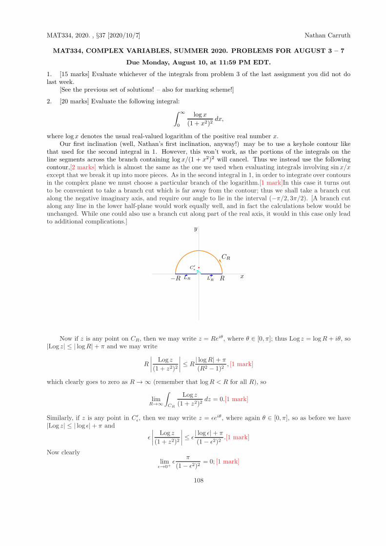
MAT334, 2020. , §37 [2020/10/7] Nathan Carruth
MAT334, COMPLEX VARIABLES, SUMMER 2020. PROBLEMS FOR AUGUST 3 – 7
Due Monday, August 10, at 11:59 PM EDT.
1. [15 marks] Evaluate whichever of the integrals from problem 3 of the last assignment you did not dolast week.
[See the previous set of solutions! – also for marking scheme!]
2. [20 marks] Evaluate the following integral:
∫ ∞
0
log x
(1 + x2)2dx,
where log x denotes the usual real-valued logarithm of the positive real number x.Our first inclination (well, Nathan’s first inclination, anyway!) may be to use a keyhole contour like
that used for the second integral in 1. However, this won’t work, as the portions of the integrals on theline segments across the branch containing log x/(1 + x2)2 will cancel. Thus we instead use the followingcontour,[2 marks] which is almost the same as the one we used when evaluating integrals involving sinx/xexcept that we break it up into more pieces. As in the second integral in 1, in order to integrate over contoursin the complex plane we must choose a particular branch of the logarithm.[1 mark]In this case it turns outto be convenient to take a branch cut which is far away from the contour; thus we shall take a branch cutalong the negative imaginary axis, and require our angle to lie in the interval (−π/2, 3π/2). [A branch cutalong any line in the lower half-plane would work equally well, and in fact the calculations below would beunchanged. While one could also use a branch cut along part of the real axis, it would in this case only leadto additional complications.]
x
y
−R RLR L′
R
CR
C′
ǫ
Now if z is any point on CR, then we may write z = Reiθ, where θ ∈ [0, π]; thus Log z = logR + iθ, so|Log z| ≤ | logR|+ π and we may write
R
∣∣∣∣
Log z
(1 + z2)2
∣∣∣∣≤ R
| logR|+ π
(R2 − 1)2, [1 mark]
which clearly goes to zero as R→ ∞ (remember that logR < R for all R), so
limR→∞
∫
CR
Log z
(1 + z2)2dz = 0.[1 mark]
Similarly, if z is any point in C′ǫ, then we may write z = ǫeiθ, where again θ ∈ [0, π], so as before we have
|Log z| ≤ | log ǫ|+ π and
ǫ
∣∣∣∣
Log z
(1 + z2)2
∣∣∣∣≤ ǫ
| log ǫ|+ π
(1− ǫ2)2.[1 mark]
Now clearly
limǫ→0+
ǫπ
(1− ǫ2)2= 0; [1 mark]
108

MAT334, 2020. , §37 [2020/10/7] Nathan Carruth
also, by L’Hopital’s rule (for real functions!),
limǫ→0+
ǫ log ǫ = limǫ→0+
log ǫ
1/ǫ= lim
ǫ→0+
1/ǫ
−1/ǫ2= lim
ǫ→0+−ǫ = 0, [1 mark]
from which we see that
limǫ→0+
∫
C′ǫ
Log z
(1 + z2)2dz = 0.
Thus, in the limits ǫ → 0+ and R → ∞, we have, since the only singularity of the integrand inside thecontour is a pole at z = i,
limǫ→0+
limR→∞
∫
L1
Log z
(1 + z2)2dz +
∫
L2
Log z
(1 + z2)2dz = 2πiResi
Log z
(1 + z2)2.[1 mark]
Before computing the residue, we note that −L1 may be parameterised as teiπ, t ∈ [0, R], so that
∫
L1
Log z
(1 + z2)2dz =
∫ R
0
log t+ iπ
(1 + t2)2dt =
∫
L2
Log z
(1 + z2)2dz + iπ
∫ R
0
1
(1 + t2)2dt.[2 marks]
Thus we have also to evaluate the integral∫ ∞
0
1
(1 + t2)2dt =
1
2
∫ ∞
−∞
1
(1 + t2)2dt;
this latter integral may be evaluated by closing the contour in the upper half-plane,[1 mark]noting that theintegral over the extra semicircle will go to zero as its radius goes to infinity since
R
∣∣∣∣
1
(1 +R2e2it)2
∣∣∣∣≤ R
1
(R2 − 1)2→ 0 as R → ∞, [1 mark]
and thus obtaining∫ ∞
−∞
1
(1 + t2)2dt = 2πiResi
1
(1 + z2)2[1 mark] = 2πi
d
dz
1
(z + i)2
∣∣∣∣z=i
= 2πi
(
− 2
(2i)3
)
=π
2, [2 marks]
so finally∫ ∞
0
1
(1 + t2)2dt =
π
4
and ∫ ∞
0
log x
(1 + x2)2dx =
1
2
[
2πiResiLog z
(1 + z2)2− i
π2
4
]
.
Thus we need only compute this residue. We have
ResiLog z
(1 + z2)2=
d
dz
Log z
(z + i)2
∣∣∣∣z=i
=1i (2i)
2 − 2(2i)Log i
(2i)4=
− 4i − 4i iπ216
=i
4+π
8, [3 marks]
whence finally∫ ∞
0
log x
(1 + x2)2dx =
1
2
[
−π2+ i
π2
4− i
π2
4
]
= −π4.[1 mark]
We note that it is reasonable to obtain a negative number since log x→ −∞ as x→ 0+.[Marking: as above.]
3. [15 marks] Suppose that f is a function which is analytic on the entire complex plane. Let CR denotethe portion of the circle of radius R centred at the origin lying between the angles θ1 and θ2 with the positivereal axis. Is it possible to have
limR→∞
∫
CR
|f(z)| ds = 0?
(The integral here is an arclength integral from multivariable calculus.) If not, prove it; otherwise, give anexample. [Hint: Liouville’s Theorem!]
109

MAT334, 2020. I, §37 [August 11] Transformations of solutions Nathan Carruth
Summary:
• We review the method of using analytic maps to perform a ‘change of variables’ in boundary-valueproblems involving Laplace’s equation.
• We give an example, and then study the properties of a few special maps.(Cf. Goursat, §§22, 24.)
38. Transformations of solutions to Laplace’s equation. Last week we discussed the Poissonkernel and its relation to the Cauchy integral theorem: we saw that, just as the Cauchy integral formula givesthe value of an analytic function everywhere inside a simple closed curve as an integral involving only thevalues of the function on the boundary of the region (i.e., the simple closed curve), so too the Poisson kernelallows us to write the values of a harmonic function inside a simple closed curve as an integral involvingonly the values of the function on the boundary (i.e., again, the curve).0 Today we shall see another methodof solving Laplace’s equation given information about the function on the boundary, using the fact thatanalytic functions essentially take harmonic functions to harmonic functions and thus allow us to perform a‘change of variables’ of sorts in Laplace’s equation to replace a (potentially) hard problem with a (hopefully)easier one.
Before beginning this, we note one small point. When we speak of harmonic functions, we always meanreal-valued functions of two real variables. On the other hand, when we speak of analytic functions onthe plane we mean complex-valued functions of a complex variable. To avoid tiresome and unimportantnotational issues, we shall agree that if u is any real-valued function of two real variables, and z ∈ C is anycomplex number, then the notation u(z) (which is technically undefined) shall mean u(Re z, Im z); in otherwords, we write as a shorthand
u(x+ iy) = u(x, y).
With this out of the way, we have the following result, which we saw some version of back towards thestart of the course: suppose that D, E ⊂ C are two regions (e.g., interiors of closed curves), that u : D → Ris a harmonic function on D, and that f : E → D is an analytic map with f(E) ∩ ∂D = ∅.1 Then the
0 It is worth noting however that there is a very basic difference between these two formulas which wehave so far glossed over: we have noted (though not proved) that the function u defined using the Poissonkernel approaches the function h in the limit as its argument (x, y) goes radially to a point on C. The sameis not in general true for the Cauchy integral formula, for a very basic reason. As we noted earlier, themethod by which we proved the Cauchy integral formula for derivatives allows us to prove also that anyfunction defined as an integral of the form
F (z) =
∫
C
h(z′)
z′ − zdz′, (1)
where C is some simply closed curve, z is any point inside C, and h is a continuous function on C, mustalso have a derivative everywhere inside C, and hence must be analytic. But this analytic function need notagree with h on the boundary curve C, for the following reason: suppose that h were real-valued; then ifF (z) = h(z) for z ∈ C, the analytic function F would be real-valued on C, and hence its imaginary partwould be zero everywhere on C. But its imaginary part must be harmonic, and any harmonic function whichvanishes on a simple closed curve must vanish everywhere inside that curve; hence F must be real-valuedinside C as well as on C, and must therefore be constant. But if h is not constant then this contradictsF (z) = h(z) on C. Another way of looking at this is that the function F includes two nonzero harmonicfunctions, so somehow the integral (1) is actually giving us two harmonic functions, which clearly containmore information on the boundary than is included in the function h alone. (I should point out that ingeneral there is no reason to believe that even the real part of F agrees with h on the boundary curve C;and here it is worth recalling that when we derived the Poisson kernel we had to add in an extra term byhand involving the point z∗.) This is a bit of a side comment, but worth keeping in mind to avoid makingmistakes.
1 In the applications we shall be mostly interested in cases where the boundary curves of D and E aresimple (i.e., where D and E are simply connected), where f(∂E) = ∂D, and where f−1 is also analytic. Butnothing in this present result relies on any of these conditions, so we state it in greater generality.
110

MAT334, 2020. I, §38 [August 11] Transformations of solutions Nathan Carruth
functionv = u ◦ f : E → R
is also harmonic on E.To see this, let a ∈ E; then f(a) ∈ D, so that u must be harmonic at f(a). Now we can find an ǫ > 0
so that the disk of radius ǫ centred at f(a) is still contained in D [we do not care whether it is containedin f(E); that is actually totally irrelevant]; let us denote this disk by U . Thus u is actually harmonic onU , and there must then be a conjugate harmonic function on U , call it u, so that u + iu is analytic on U .(See Goursat, §3, p. 10; or §9 in these lecture notes.) Let us denote this function by g. Then g ◦ f must beanalytic at a, by the chain rule; but since the real and imaginary parts of all analytic functions are harmonic,its real part u◦f = v must be harmonic on E, as desired. (The restricting to a disk is only to make sure thatthe function u is well-defined – as we have seen before (e.g., in the second quiz), on a non-simply connectedregion a conjugate harmonic function may become multiple-valued.)
For the applications, we need to restrict the regions E and D and the function f , and for this we need abit more notation. We shall require E and D to be simply connected; equivalently, we require their boundarycurves ∂D and ∂E to be simple closed curves. We shall also require E and D to represent only the interiorof their boundary curves, i.e., that E ∩ ∂E = D ∩ ∂D = ∅; we set E = E ∪ ∂E, D = D ∪ ∂D.2 We assumethat f−1 : D → E (exists and) is analytic, and that f and f−1 extend to continuous functions mapping Eto D and D to E, respectively; at the risk of being extremely confusing, we shall denote these extensions byf and f−1 as well.
To put all of this more simply, we assume that f is invertible with analytic inverse, and that f and itsinverse extend to continuous functions on the boundary of E and D, respectively.
Now suppose that u satisfies∆u = 0 on D, u|∂D = h, (2)
where h is some piecewise-continuous function on ∂D. We call any problem like (2) a boundary-value problem,since we have conditions on u on the boundary of the region. Now let E and f : E → D satisfy the conditionsjust described, and set v = u ◦ f . Then v is harmonic on E, while if a ∈ ∂E we must have f(a) ∈ ∂D, sothat
v(a) = (u ◦ f)(a) = u[f(a)] = h[f(a)]
by the boundary condition in (2). Thus v satisfies the boundary-value problem
∆v = 0 on E, v|∂E = h ◦ f. (3)
Now it may happen that we can find E and f such that problem (3) is simpler than (2); in fact, in theexamples we shall see the answer to (3) can be guessed at quite easily. Suppose thus that we can find somefunction v satisfying (3). Then running the above logic backwards, we see that the function u = v ◦ f−1
must satisfy the boundary-value problem
∆u = 0 on D, u|∂D = h;
in other words, u is a solution to our original boundary value problem (2).Let us see an example.
EXAMPLE. Solve the following boundary problem on the region D given in polar coordinates as D ={(r, θ) | r ∈ (0, 1), θ ∈ (−π/4, π/4)}:
∆u = 0 on D, u|∂D =
sin 2θ, r = 1r2, θ = π/4−r2, θ = −π/4
(4)
The factor of 2 in the sine, the square in ±r2, and the shape of the region suggest that perhaps f oughtto have something to do with a square. Now z 7→ z2 increases the angle by a factor of 2; thus if we were to
2 For those who know something of topology, we note that E and D, as the notation suggests, are justthe closure of E and D in the usual topology of R2 in this case.
111

MAT334, 2020. I, §38 [August 11] Transformations of solutions Nathan Carruth
take f(z) = z2, the region E would be even narrower than the region D, and the problem would probablynot be any simpler. If we take f(z) = z1/2, though (assuming we can take an appropriate branch!), then wesee that the region E would be a half-disk. Thus let us let f(z) = z1/2, where we take a branch cut alongthe negative real axis and require θ ∈ (−π, π). Then if we set
E = {(r, θ) | r ∈ (0, 1), θ ∈ (−π/2, π/2)},
we see that f : E → D is one-to-one and onto, and its inverse is given by z 7→ z2, which is analytic on D.Further, we may extend f to a continuous function on E by setting f(0) = 0 (this will not extend to ananalytic function, of course, but that does not matter). Now we must determine how the boundary conditionchanges; in other words, if we define h : ∂D → R by
h =
sin 2θ, r = 1r2, θ = π/4−r2, θ = −π/4
,
then we need to determine h ◦ f : ∂E → R. Now ∂E also has three pieces, namely r = 1, θ ∈ [−π/2, π/2],θ = π/2, r ∈ [0, 1], and θ = −π/2, r ∈ [0, 1]. Now if z = reiθ , where θ ∈ (−π, π), then f(z) = r1/2e
12iθ; thus
these three boundary pieces are mapped to, respectively,
r = 1, θ ∈ [−π/4, π/4]; θ = π/4, r ∈ [0, 1]; θ = −π/4, r ∈ [0, 1].
Now if r = 1 and θ ∈ [−π/2, π/2], then we have r1/2 = 1 and
(h ◦ f)(reiθ) = h(r1/2e12iθ) = h(e
12iθ) = sin 2 ·
(1
2θ
)
= sin θ;
if θ = π/2 and r ∈ [0, 1], then we have 12θ = π/4 and
(h ◦ f)(reiθ) = h(r1/2e12iθ) =
(
r1/2)2
= r;
finally, if θ = −π/2 and r ∈ [0, 1], then we have 12θ = −π/4 and
(h ◦ f)(reiθ) = h(r1/2e12iθ) = −
(
r1/2)2
= −r.
Pulling this together, we have
h ◦ f =
sin θ, r = 1r, θ = π/2−r, θ = −π/2
,
so that we wish to solve the problem
∆v = 0 on E, v|∂E =
sin θ, r = 1r, θ = π/2−r, θ = −π/2
(5)
Now we note that if a, b, and c are real numbers, then the function
g(x, y) = a+ bx+ cy (6)
will be harmonic at every point (x, y) ∈ R2, since all of its second order derivatives vanish. Let us seewhether we can find a solution to (5) which is of this form. The idea is that, since all of these functionssatisfy Laplace’s equation, we only need to fit the boundary conditions. Now in polar coordinates, thefunction g may be written
g = a+ br cos θ + cr sin θ.
112

MAT334, 2020. I, §38 [August 11] Transformations of solutions Nathan Carruth
If r = 1, this gives a + b cos θ + c sin θ, which will fit the boundary condition in (5) if a = b = 0, c = 1; ifθ = ±π/2, then it gives
a± cr,
which will also fit the boundary condition in (5) if a = 0 and c = 1. In other words, we have found that thefunction
v(x, y) = y
is a solution to (5).Working backwards, then, we know from our general work above that the function u = v ◦f−1 will solve
our original problem. Now f−1(z) = z2, so that we have finally the solution
u(x, y) = v[f(x+ iy)] = v(x2 − y2, 2xy) = 2xy
to the boundary value problem (4).If we step back and look at the broad sweep of the logic used in this example, we see that to make
efficacious use of this technique in practice, we must have a catalogue of two things: one, transformationsand regions; two, standard solutions to Laplace’s equation on the domain regions of these transformations.For us, the main class of standard solutions will be the linear ones given in (6). We now describe a fewelementary transformations which are useful.EXAMPLES of transformations and regions useful for solving Laplace’s equation.
1. Powers and roots on wedges. If n ∈ Z, n > 0, then the map z 7→ zn takes a wedge with vertex at theorigin with angle α to another wedge with vertex at the origin with angle nα. For this transformation tobe invertible, the angle α must be less than 2π/n. Similarly, if n ∈ Z, n > 0, then the map z 7→ z1/n, aftertaking an appropriate branch, will map a wedge of angle α with vertex at the origin to another wedge withvertex at the origin and angle α/n, assuming that α < 2π. Wedges have three boundaries, two of which arelines and the third of which is a circular arc; on the circular arc, a map z 7→ zp (p = n or p = 1/n, as thecase may be) will take a point reiθ to a point rpeipθ, i.e., it will multiply the angle θ by p (where θ mustbe in the range corresponding to the chosen branch if p = 1/n), while on the lines the map acts by simpleexponentiation, as in the example above.
2. Inversion. The map z 7→ z−1, as we have seen before (see §16 of these lecture notes), takes thepunctured plane into itself, but ‘turns it inside out’ by mapping the region outside the unit circle to theregion inside the unit circle.
3. The exponential function. Consider the map z 7→ ez. We have seen already (see the solutions tothe first homework assignment) that this map takes lines parallel to the real axis to rays from the origin,and lines parallel to the imaginary axis to circles centred at the origin. Thus this map will take certainrectangular regions in the plane into annular wedges. (Going further, to whole annular regions or even a fulldisk, would involve extra considerations beyond the scope of our present discussion.)
4. The maps z 7→ sin z and z 7→ cos z. The second of these has already been described in some detailin §16 of these lecture notes (cf. Goursat, §22); in particular, it was shown there that z 7→ cos z takes therectangle {x+ iy |x ∈ (0, π), y ∈ (0,+∞)} into the lower half-plane {x+ iy | y < 0}. Let us see a bit morecarefully what it does on the boundary of this rectangle. This boundary consists of three lines, the half-linex = 0, y ≥ 0, the line segment y = 0, x ∈ [0, π], and the half-line x = π, y ≥ 0. Let us consider these inturn. We have (see, e.g., §13 of these notes)
cos(x+ iy) = cosx cosh y − i sinx sinh y;
thus if x = 0 we havecos(iy) = cosh y,
which takes the interval [0,+∞) into the interval [1,+∞) in a one-to-one fashion. Similarly, if x = π, thenwe have
cos(π + iy) = − cosh y,
which takes the interval [0,+∞) into the interval (−∞,−1]. Finally, if y = 0, cos z will be just the ordinaryreal-valued function cosx, which takes the interval [0, π] into the interval [−1, 1] (though in reverse order,
113

MAT334, 2020. I, §38 [August 11] Transformations of solutions Nathan Carruth
i.e., it is decreasing on that interval). All told, then, the half-line x = 0, y ≥ 0 will map to the interval[1,+∞), the segment y = 0, x ∈ [0, π] will map to the interval [−1, 1] (where the point 1 is mapped from theintersection x = y = 0 of these two parts of the boundary) and finally the half-line x = π, y ≥ 0 will map tothe interval (−∞,−1], with as before the point −1 is mapped from the intersection x = π, y = 0 of theselast two parts of the boundary. This suggests that this map may be useful if we are interested in findingsolutions to problems on the lower half-plane whose initial data can be broken down in some way across thethree intervals (−∞,−1], [−1, 1], and [1,+∞).
We note one other result: if x = π/2, then we have
cos(x+ iy) = cos(π/2 + iy) = −i sinh y,
from which we see that the half-line x = π/2, y ≥ 0 is mapped to the negative imaginary axis. This means,incidentally, that the two rectangles
{x+ iy |x ∈ (0, π/2), y > 0}, {x+ iy |x ∈ (π/2, π), y > 0}
map to the fourth and third quadrants, respectively (since cosx > 0 for x ∈ (0, π/2) and cosx < 0 forx ∈ (0, π/2)). Thus this map can also be used for problems on a quarter-plane.
Similarly, let us consider the map z 7→ sin z. We have (ibid.)
sin(x + iy) = sinx cosh y + i cosx sinh y.
In this case we take as our domain the rectangular strip {x + iy |x ∈ (−π/2, π/2), y > 0}, since sinx isinvertible on (−π/2, π/2) but not on any strictly larger interval. Let us consider the values of sin on thethree boundary lines as we did for cos. If x = −π/2, then we have
sin(−π/2 + iy) = − cosh y,
while if x = π/2 then we havesin(π/2 + iy) = cosh y;
thus these two lines map to the segments (−∞,−1] and [1,+∞), similarly to what we found for cos (exceptnote that the order is reversed). Similarly, if y = 0 then sin z is just the ordinary real-valued sine functionsinx, which maps the interval [−π/2, π/2] to the interval [−1, 1]. Thus, again, the boundary is mapped ontothe entire real line. Since cosx and sinh y are both positive everywhere on the rectangle, we see that sinmaps the rectangle into the upper half-plane; and this map is actually onto. Again, as with cos, we see thatthe midline x = 0, y ≥ 0 maps to the positive real axis, and we see further that the rectangles
{x+ iy |x ∈ (−π/2, 0), y > 0}, {x+ iy |x ∈ (0, π/2) y > 0}
map to the second and first quadrants, respectively (again, which quadrant is the image of which rectanglecan be determined from the sign of x).
114

MAT334, 2020. I, §38 [August 13] L’Hopital’s rule Nathan Carruth
Summary:• We give a proof of L’Hopital’s rule for analytic functions.• We then show how another class of boundary conditions for Laplace’s equation transforms under analyticmaps, and give an example.
• [For the material on analytic continuation, please see the pre-class notes.]39. L’Hopital’s rule for analytic functions. We prove the following version of L’Hopital’s rule for
analytic functions. Suppose that f and g are analytic near a point a, and that both f and g have a zero oforder m at a. Then
limz→a
f(z)
g(z)= lim
z→a
f (m)(z)
g(m)(z). (1)
(In the terminology usually used to discuss L’Hopital’s rule in elementary calculus courses, this is a limit oftype 0/0.)
To see this, note that since f and g have zeroes of order m at a, there are functions φ(z) and γ(z) whichare both analytic and nonzero near a and satisfy
f(z) = (z − a)mφ(z), g(z) = (z − a)mγ(z).
Moreover, we claim that φ(a) = f (m)(a)/m! and γ(a) = g(m)(a)/m!. The proof of these two equations is thesame so we show only the first one. There are two distinct ways of doing this. The one we used in lectureinvolved Taylor series and is as follows. Suppose that the Taylor series for φ at a is
∞∑
k=0
ak(z − a)k,
where we know that a0 = φ(a) 6= 0. Then the Taylor series for f at a is
∞∑
k=0
ak(z − a)k+m.
But this series must equal∞∑
n=0
1
n!f (n)(a)(z − a)n;
equating coefficients of like powers, we see that
a0 =1
m!f (m)(a),
as claimed.The second method is much quicker and involves the Cauchy integral formula: if C is a sufficiently small
circle around a, then we have
φ(a) =1
2πi
∫
C
φ(z′)
z′ − adz′
=1
2πi
∫
C
f(z′)/(z′ − a)m
z′ − adz′ =
1
2πi
∫
C
f(z′)
(z′ − a)m+1dz′
=1
m!f (m)(a),
by the Cauchy integral formula for derivatives.Given this, the proof of (1) is easy:
limz→a
f(z)
g(z)= lim
z→a
(z − a)mφ(z)
(z − a)mγ(z)= lim
z→a
φ(z)
γ(z)=φ(a)
γ(a)=f (m)(a)
g(m)(a),
115

MAT334, 2020. I, §39 [August 13] Neumann boundary conditions Nathan Carruth
since the factors of m! will cancel.We can also use the inner workings of the above proof to evaluate limits, which is often much easier
than applying the result itself, as the following example shows.EXAMPLE. Let n ∈ Z be positive. Find
limx→0
(sinx)2n
(1 − cosx)n.
Let us consider the corresponding complex limit, i.e., replace the real number x in the limit above by acomplex number z, since if the resulting limit exists then certainly the original limit does as well. Now notethat sin z has a zero of order 1 at 0, so that we may write
sin z = zφ(z)
for some function φ which will be analytic and nonzero at z = 0 (and hence everywhere in this case, thoughthat is not important). In fact, of course, the function φ will simply be the function
{sin z/z, z 6= 0
1, z = 0
which we have seen many times already. We have moreover that φ(0) = ddz sin z
∣∣z=0
= 1. Further, since
cos z = 1− 1
2z2 + · · · , (2)
we see that 1− cos z has a zero of order 2 at 0, so we may write
1− cos z = z2γ(z),
where by inspection of the series (2) we have γ(0) = 12 . (This could also be obtained by differentiating as in
the proof above, of course; in that case the factor of 1/2 comes from the 1/m!.) Thus we may write
limz→0
(sin z)2n
(1− cos z)n= lim
z→0
z2n[φ(z)]2n
z2n[γ(z)]n
= limz→0
[φ(z)]2n
[γ(z)]n=
[φ(0)]2n
[γ(0)]n= 2n.
To apply L’Hopital’s rule to this directly would have required us to differentiate n times, which would beextremely messy. This demonstrates the utility of power series manipulations and other concepts (such asthe order of a zero) which we have studied in this course in elucidating the behaviour of analytic functions.
40. Transformation of Neumann boundary conditions by analytic maps. So far we haveconsidered only problems involving so-called Dirichlet boundary conditions, i.e.,
∆u = 0 on D, u|∂D = h. (3)
This means, of course, that we seek a function u which satisfies Laplace’s equation inside the region D andis equal to the function h on the boundary of D; note that the Laplacian of u need not be defined on theboundary of D. Another type of boundary condition we could give is that the normal deriviative of u onthe boundary be equal to some given function. In other words, let n denote the unit outward normal tothe boundary curve ∂D (this is defined in an analogous way to how one defines the outward unit normal toa region in three-dimensional space when one discusses the divergence theorem in multivariable calculus);then, writing
∂u
∂n= n · ∇u
(i.e., we define ∂u/∂n to be the quantity on the right-hand side), we may consider the problem
∆u = 0 on D,∂u
∂n
∣∣∣∣∂D
= h, (4)
116

MAT334, 2020. I, §40 [August 13] Neumann boundary conditions Nathan Carruth
where again h is some function on the boundary ∂D. Note first of all that this problem will not have aunique solution on D, since if u is any solution then clearly so also is u+C, where C is any real number; thusin order to get a unique solution we need to specify some other piece of information about u, for example,its value at some point. We shall assume that given the value of u at any point, (4) has a unique solution.We shall also restrict attention to the case h = 0.
Let us see whether our method of transforming the problem with an analytic function is applicable toproblem (4). Thus consider a region E and an analytic function f : E → D satisfying the conditions given in§38 of these lecture notes, and consider problem (4) with h = 0. We claim that if v = u ◦ f , then v satisfiesthe problem
∆v = 0 on E,∂v
∂N
∣∣∣∣∂E
= 0, (5)
where ∂/∂N denotes the derivative of v in the direction normal to E. Let us see why this is so. That vsatisfies ∆v = 0 has already been shown; thus we need only consider the boundary condition. Let a ∈ E.Let N denote the outward unit normal to E at a; then
∂v
∂N
∣∣∣∣a
= N · ∇v(a) = N · ∇(u ◦ f)(a).
Now let b = f(a) and consider ∇u(b). If ∇u(b) = 0, then it is not hard to show that ∇(u ◦ f)(a) = 0(using the chain rule); thus in this particular case ∂v/∂N |a will be zero, as claimed. Thus now suppose that∇u(b) 6= 0. Since
∂u
∂n
∣∣∣∣b
= n · ∇u(b) = 0,
where n denotes the outward unit normal to D at b = f(a), we see that ∇u(b) must be perpendicular to n.But now ∇u(b) must also be perpendicular to the level curve, call it C, of u which passes through b, i.e., tothe set of points (x, y) satisfying u(x, y) = u(b); since we are in the plane this implies that this level curvemust be tangent to n and hence perpendicular to the boundary curve ∂D. But since f−1 is assumed to beanalytic and therefore conformal (its derivative will be nonzero since it is invertible), and maps ∂D to ∂E,this means that the curve C′ to which f−1 maps C must be perpendicular to the boundary ∂E at the pointa. But this curve is just the level curve of v through a, for (x, y) satisfies v(x, y) = v(a) if and only if
u[f(x, y)] = u[f(a)] = u(b),
i.e., if and only if f(x+iy) = x′+iy′ for some point (x′, y′) in C, which is equivalent to x+iy = f−1(x′+iy′),i.e., that (x, y) lie on C′. Thus the level curve of v through a must be perpendicular to the boundary ∂E,which means as before that the gradient of v at a must be perpendicular to the normal vector N, and hence
∂v
∂N
∣∣∣∣a
= N · ∇v(a) = 0,
so that v satisfies the boundary condition in (5), as claimed.Before going into the example, recall that the map z 7→ sin z was described at the end of §38 in the
previous set of lecture notes.EXAMPLE. Let U = {(x, y)|y > 0} denote the upper half-plane. Solve the following problem:
∆u = 0 on U, u|∂U =
{0, x ∈ (−∞,−1)1 x ∈ (1,∞)
,∂u
∂n
∣∣∣∣∂U
= 0 if x ∈ [−1, 1]; (6)
in other words, we require u to be 0 on the real axis except on the interval [−1, 1], and we require ∂u/∂n tobe zero on this interval. Now geometrically it is clear that ∂u/∂n = −∂u/∂y, so that this is equivalent torequiring ∂u/∂y to vanish on this interval.
Now of the conformal maps listed at the end of §38, the only one which maps onto the upper half-planeis z 7→ sin z, where we take z to lie in the rectangle
R = {(x, y)|x ∈ (−π/2, π/2), y > 0}.
117
MAT334, 2020. I, §40 [August 13] Neumann boundary conditions Nathan Carruth
Thus we consider transforming the problem (6) using this map. Let v(z) = u[sin(z)]; then v must satisfy theproblem
∇v = 0 on R, v(−π/2, y) = 0, v(π/2, y) = 1,∂v
∂N
∣∣∣∣(x,0)
= 0, x ∈ (−π/2, π/2), (7)
where here ∂/∂N denotes the outward normal derivative of v; but as before this is just −∂/∂y, so that thislast condition gives simply
∂v
∂y
∣∣∣∣(x,0)
= 0, x ∈ (−π/2, π/2).
Thus we must now find a function v which satisfies (7). Since the only real class of solutions we have onrectangles are the linear ones, let us see whether this problem has a linear solution; in other words, let ussee whether we can find numbers a, b, and c such that
v(x, y) = a+ bx+ cy
(which will automatically satisfy ∆u = 0) satisfies the boundary conditions. The conditions on x = ±π/2give
0 = v(−π/2, y) = a− bπ/2 + cy, 1 = v(π/2, y) = a+ bπ/2 + cy,
whence we see immediately that c = 0 (as otherwise the right-hand sides of these expressions would dependon y while the left-hand sides clearly do not) and are thus left with the system
a− π
2b = 0
a+π
2b = 1.
Adding these equations gives a = 1/2, while subtracting the first from the second gives b = 1/π; thus thefunction
v =1
2+
1
πx
will indeed satisfy the boundary conditions on x = ±π/2, a fact which can readily be verified by directsubstitution. Note that this solution satisfies also ∂v/∂y = 0 everywhere, and hence in particular on thesegment {(x, 0) |x ∈ (−1, 1)}, which is the final boundary condition in (7). Thus v is the solution to (7).
This means that the solution to the original problem will be u = v ◦ arcsin z. Now if we write a pointin the plane in complex notation, then we have v(x + iy) = 1
2 + 1πx = 1
2 + 1πRe (x + iy); thus we need to
determine Re arcsin z, where z is in the upper half-plane and the branch of arcsin taken is that which mapsinto the rectangle R. We could determine this using the formula for arcsin which we found previously, but itseems easier to proceed in a different way. Let z = a+ ib be in the upper half-plane, and let w = x+ iy ∈ Rsatisfy sinw = z; in other words,
sinw = sinx cosh y + i cosx sinh y = a+ ib,
and we note that b > 0, which implies that x ∈ (−π/2, π/2) and y > 0. We wish to find Rew = x. Now aswe just saw, b > 0 implies cosx > 0. Further, sinx = 0 exactly when a = 0, and in this case we must havex = 0. Thus for us Re arcsin0 = 0, and we may assume that a 6= 0. Now let α = sin2 x. Then cos2 x = 1−α,so that we have
a2
α+
b2
α− 1=
a2
sin2 x− b2
cos2 x= cosh2 y − sinh2 y = 1;
if we multiply through by α(α− 1), this gives
α2 − α = a2(α− 1) + αb2 = α(a2 + b2)− a2
α2 − (1 + a2 + b2)α+ a2 = 0
118

MAT334, 2020. I, §40 [August 13] Neumann boundary conditions Nathan Carruth
whence applying the quadratic formula, we obtain
α =1
2
[
1 + a2 + b2 ±√
(1 + a2 + b2)2 − 4a2]
. (8)
That the quantity inside the square root is always positive can be seen as follows:
(1 + a2 + b2)2 − 4a2 = 1 + 2a2 + 2b2 + a4 + 2a2b2 + b4 − 4a2
= b2(b2 + 2) + a4 − 2a2 + 1 + 2a2b2 = b2(b2 + 2) + 2a2b2 + (a2 − 1)2,
which is a sum of positive (since b 6= 0) and nonnegative quantities and therefore positive. Now note thatboth roots above are nonnegative, since
√
(1 + a2 + b2)2 − 4a2 ≤ 1 + a2 + b2. We claim that the + root in(8), which we denote by α+, must be greater than 1. To see this, note that since b > 0
4− 4(1 + b2) = −4b2 < 0;
thus
(1 + b2 + a2)2 − 4a2 > (1 + b2 + a2)2 − 4(a2 + b2) = (1 + b2 + a2)2 − 4(1+ a2 + b2) + 4 = [(1 + b2 + a2)− 2]2,
so √
(1 + b2 + a2)2 − 4a2 >∣∣1 + b2 + a2 − 2
∣∣ .
Now if 1 + b2 + a2 > 2, then clearly α+ > 1; while if 1 + b2 + a2 ≤ 2, then by the above inequality we have√
(1 + b2 + a2)2 − 4a2 > 2− (1 + b2 + a2), (1 + b2 + a2) +√
(1 + b2 + a2)2 − 4a2 > 2,
and again α+ > 1. Thus in any event we must have α+ > 1, as desired. Since we require α = sin2 x for xreal, we are only interested in values of α that lie in [0, 1], and we therefore reject the value α+ and take
α = 12
[
1 + a2 + b2 −√
(1 + a2 + b2)2 − 4a2]
. We claim that α < 1. This can be seen as follows:
2α = 1 + a2 + b2 −√
(1 + a2 + b2)2 − 4a2 =(1 + a2 + b2)2 − [(1 + a2 + b2)2 − 4a2]
1 + a2 + b2 +√
(1 + a2 + b2)2 − 4a2
=4a2
1 + a2 + b2 +√
b2(b2 + 2) + 2a2b2 + (a2 − 1)2<
4a2
1 + a2 + b2 + a2 − 1<
4a2
2a2= 2,
giving α < 1, as desired. (Here we have used b > 0 to conclude that√
b2(b2 + 2) + 2a2b2 + (a2 − 1)2 >√
(a2 − 1)2 = |a2 − 1| ≥ a2 − 1.) This gives, finally, then,
x = Re arcsin z = ± arcsin
√
1
2
[
1 + a2 + b2 −√
(1 + a2 + b2)2 − 4a2]
,
where here arcsin denotes the ordinary inverse sine of a number in the interval [0, 1), lying in [0, π/2). Wewill take the + sign for a ≥ 0 and the − for a ≤ 0; a = 0 clearly gives x = 0, so in this case it does notmatter which sign we take. Our solution is then finally
u(x, y) =1
2+
1
π·
arcsin
√
12
[
1 + x2 + y2 −√
(1 + x2 + y2)2 − 4x2]
, x ≥ 0
− arcsin
√
12
[
1 + x2 + y2 −√
(1 + x2 + y2)2 − 4x2]
, x ≤ 0
. (9)
It is instructive to see how this solution satisfies the boundary conditions. Suppose y = 0; then theformula above gives3
1 + x2 + y2 −√
(1 + x2 + y2)2 − 4x2 = 1 + x2 −√
(1 − x2)2 = 1 + x2 − |1− x2|.3 Technically, of course, we should be considering rather the limit as y → 0+. The formula above will
clearly be continuous at y = 0, however, if it is defined at y = 0; and thus it suffices to show that it is definedat y = 0, which is afforded by our following calculation.
119

MAT334, 2020. I, §40 [August 13] Neumann boundary conditions Nathan Carruth
Now if x ∈ [−1, 1], this gives 1 + x2 − (1 − x2) = 2x2, while if x ∈ (−∞,−1) ∪ (1,+∞) it gives instead1 + x2 − (x2 − 1) = 2. Thus
arcsin
√
1
2
[
1 + x2 + y2 −√
(1 + x2 + y2)2 − 4x2]
=
{arcsin |x|, x ∈ [−1, 1]
π2 , x ∈ (−∞,−1) ∪ (∞, 1)
,
where the second line follows from arcsin 1 = π/2. If we substitute this back into (9), we thus obtain (usingthe fact that arcsin is odd)
u(x, 0) =1
2+
1
π
−π2 , x ∈ (−∞,−1)
arcsinx, x ∈ [−1, 1]π2 , x ∈ (1,+∞)
=
0, x ∈ (−∞,−1)12 + 1
π arcsinx, x ∈ [−1, 1]1, x ∈ (1,+∞)
,
which clearly satisfies the boundary conditions on (−∞,−1) ∪ (∞, 1). That the remaining condition on(−1, 1) holds, we leave to the intrepid reader; it follows fairly simply from the observation that
∂
∂y
[
1 + x2 + y2 −√
(1 + x2 + y2)2 − 4x2]
= 2y − 2y(1 + x2 + y2)[(1 + x2 + y2)2 − 4x2]−1/2,
and the observation that this quantity vanishes as y → 0+ for all x ∈ (−1, 1). (This is clear, since theexpression inside the exponent is positive for all such x even when y = 0, by the foregoing.)
120

MAT334, 2020. , §40 [2020/10/7] Nathan Carruth
MAT334, COMPLEX VARIABLES, SUMMER 2020. PROBLEMS FOR AUGUST 10 – 14
Due Friday, August 14, at 11:59 PM EDT.
1. [15 marks; modified version of Question 3 from last week’s assignment.] Suppose that f is a nonzerofunction which is analytic on the entire complex plane. (‘Nonzero’ here means that there is some point inthe complex plane at which f is not zero. It does not mean that f has no zeros in the plane.) Let CR denotethe (full) circle of radius R centred at the origin. Is it possible to have
limR→∞
∫
CR
|f(z)| ds = 0?
(The integral here is an arclength integral from multivariable calculus.) If not, prove it; otherwise, give anexample. [Hint: check the proof of Liouville’s Theorem (the one in the lecture notes)!]
We may proceed as in the proof of Liouville’s Theorem in the lecture notes. Let z0 ∈ C[1 mark], andlet R > |z0|+1[2 marks]. By the Cauchy integral formula, we have, letting CR denote the circle of radius Rcentred at the origin[1 mark],
|f(z0)| =∣∣∣∣
1
2πi
∫
CR
f(z)
z − z0dz
∣∣∣∣[1 mark] ≤ 1
2π
∫
CR
∣∣∣∣
f(z)
z − z0
∣∣∣∣ds[2 marks] ≤ 1
2π
∫
CR
|f(z)| ds[1 mark],
since if z is on CR then |z − z0| ≥ 1[2 marks]. But if we now take R to infinity, this last integral mustvanish[1 mark], giving |f(z0)| = 0[1 mark], or f(z0) = 0[1 mark]. But z0 ∈ C was arbitrary[1 mark], so fmust be identically zero[1 mark].[Marking: as above. Another method would be to show that all of the coefficients of the Taylor series off vanish at the origin – this would be much closer to the proof of Liouville’s Theorem in Goursat. On theother hand, the vanishing of the integral does not imply directly that the modulus of f must be bounded –if you said that you may have gotten very few marks.]
2. [10 marks] (a) Show that for all z = x+ iy ∈ C,
| sin z| ≤ e|y|.
Let z = x+ iy; then
| sin z| =∣∣∣∣
eiz − e−iz
2i
∣∣∣∣[1 mark] ≤ 1
2
(∣∣eix+y
∣∣+∣∣e−ix+y
∣∣)[1 mark] ≤ 1
2
(e−y + ey
)[1 mark] ≤ e|y|[1 mark].
(b) Using part (a) and Rouche’s Theorem, determine how many zeros the function
3z8 + sin z
has in the unit disk. [It is worth spending some time thinking about whether the same procedure can beapplied on arbitrarily large disks. But you do not need to say anything about that in your solution.]
If z = x+ iy is any point on the unit circle[1 mark], we ahve |y| ≤ 1[1 mark], so
∣∣3z8
∣∣ = 3 ≥ e ≥ e|y| ≥ | sin z|, [1 mark]
and by Roche’s Theorem the function 3z8 + sin z must have as many zeroes as 3z8[1 mark] (countingmultiplicities[1 mark]), i.e., 8.[1 mark][Marking: as above.]
3. [10 marks] (a) Find a polynomial solution to the following problem on the unit disk D = {z | |z| < 1}:
∆u = 0, u|∂D = cos θ,
where θ is the usual polar coordinate on the plane.
121

MAT334, 2020. , §40 [2020/10/7] Nathan Carruth
We look for a linear solution of the form u = a+ bx+ cy[1 mark]. On the unit circle, we have x = cos θ,y = sin θ[1 mark]; thus we require
a+ b cos θ + c sin θ = cos θ, [1 mark]
from which we see that a = c = 0, b = 1[1 mark]. Thus u = x will solve the given problem.[1 mark](b) Use your solution to (a) and a conformal transformation to solve the following problem on the
exterior of the unit disk, i.e., the set E = {z | |z| > 1}:
∆u = 0, u|∂E = cos θ, u→ 0 as |z| → ∞.
(Note that ∂E = ∂D, both being just the unit circle.)The function z 7→ 1/z will take the interior of the unit circle (without the origin) to the exterior[1 mark];
thus the function (setting z = x+ iy)
v(x, y) = u(1/z) = u
(x− iy
x2 + y2
)
=x
x2 + y2[1 mark]
will be harmonic on the exterior of the unit disk[1 mark]. Since on the unit disk it satisfies
v =cos θ
cos2 θ + sin2 θ= cos θ, [1 mark]
and if z = R(cos θ + i sin θ), R > 0, it is
v =R cos θ
R2=
1
Rcos θ[1 mark]
which goes to zero as |R| = z → ∞, this v must be the solution to our problem.[Marking: as above.]
4. [15 marks] Solve the following problem on the lower half-plane H = {x+ iy | y < 0}:
∆u = 0, u|∂H =
π, x < −1cos−1 x, x ∈ (−1, 1)
0, x > 1
(Note that ∂H , the boundary of H , is just the real axis.)We transform this problem using the map z 7→ cos z[1 mark] from the rectangle R = {x + iy |x ∈
(0, π), y > 0}[1 mark] to the lower half-plane. We must determine the new boundary data. The linex = 0, y > 0 is mapped to the interval (1,+∞), on which u is 0; thus the transformed data will also be 0there[1 mark]. Similarly, the line x = π, y > 0 is mapped to the segment (−∞,−1), on which u is π; thusthe transformed ata must be 1 there[1 mark]. Finally, on the segment y = 0, x ∈ (0, π), we have
cos z = cosx,
i.e., the point (x, 0) is mapped to (cosx, 0)[1 mark], so
u(cos z) = u(cosx, 0) = arccos cosx = x[1 mark]
since we are using the branch of arccos which takes [−1, 1] into [0, π], and x ∈ (0, π). Thus the transformedproblem is
∆v = 0 on R, v|∂R =
0, x = 0x, y = 0π, x = π
.[1 mark]
122
MAT334, 2020. , §40 [2020/10/7] Nathan Carruth
We seek a linear solution to this problem; thus we write v = a+ bx + cy[1 mark], and try to solve for a, b,and c, using the boundary conditions. These give
a+ cy = 0
a+ bx = x
a+ bπ + cy = π;
[2 marks]
ince these must hold for all x and y, we have a = c = 0, b = 1[2 marks], so v = x[1 mark]. More carefully,we have v(x, y) = x, or v(x + iy) = x, so v(z) = Re z. Thus u(z) = (v ◦ arccos)(z) = Re arccos z[1 mark].We may express this in terms of Re arcsin z as follows[1 mark]. We have the formula
sin(w + π/2) = cosw;
thus if w = arccos z we havez = cosw = sin(w + π/2),
so w = arcsin z − π/2, at least if we take the right branch of arcsin. Now the branch of arccos we use mapsinto [0, π], while the branch of arcsin used in the notes maps into [−π/2, π/2]; thus we must replace arcsinby π − arcsin, meaning that we have finally the solution
u(z) =π
2− Re arcsin z.
[Marking: as above. This exercise is quite close to the example on pp. 3 – 6 of the August 13 lecture noteson the course website.]
123

MAT334, Summer 2020 Final assessment solutions and rubric
1. [9 marks] Suppose that f is a function which is analytic on the entire complex plane, and that there isa constant C > 0 such that |f(z)| ≤ CR whenever |z| = R. If f(0) = 0 and f ′(0) = 1, what is f?
We note that f may be written as
f(z) = z +
∞∑
n=2
anzn, [2 marks]
where
an =1
2πi
∫
CR
f(z′)
z′n+1dz′, [1 mark]
CR being a circle of radius R about the origin. But now
|an| =∣∣∣∣
1
2πi
∫
CR
f(z′)
z′n+1dz′∣∣∣∣≤ 1
2π
∫
CR
|f(z′)|Rn+1
ds ≤ 1
2π
∫ 2π
0
CR
Rn+1Rdt[2 marks] =
C
Rn−1[1 mark]
which goes to zero as R → ∞ if n ≥ 2[1 mark]. Since an does not depend on R, we must have an = 0 forn ≥ 2[1 mark]; thus f(z) = z[1 mark].
2. [7 marks] How many zeroes does the function znez + 12 sin z, also on the unit disk?
We note that on the unit circle, 18 | sin z| ≤ 1
8e|y| ≤ e/8[2 marks], while |znez| = |ez| = ex ≥ e−1 >
18e[2 marks], so that by Rouche’s Theorem[1 mark], znez + 1
8 sin z has the same number of zeroes in the unitdisk as znez[1 mark], namely n[1 mark].
3. [6 marks] Using the Taylor series for ez around z = 0, find the Laurent series for e1/z around z = 0.Use this to determine
∫
C e1/z dz, where C is any circle centred at the origin.
We have
ez =
∞∑
n=0
1
n!zn[1 mark],
so for z 6= 0
e1/z =
∞∑
n=0
1
n!z−n[1 mark].
Thus∫
C
e1/z dz =∞∑
n=0
1
n!
∫
C
z−n dz = 2πi[2 marks],
since only the n = 1 term contributes[2 marks], as we have seen many times during the course.
Evaluate the following integrals.4. [10 marks]
∫ +∞
−∞
e−ix
(x2 + 4x+ 8)2dx.
Since we have a factor of e−ix in the numerator, we must close in the lower half-plane. We will use thecontour shown in the figure[1 mark]. Now z2 + 4z + 8 = 0 gives z = −2 + 1
2 (16− 32)1/2 = −2± 2i[1 mark],so in the lower half-plane we have only one pole, at −2 − 2i[1 mark]. Now since for R sufficiently large wehave
1
|z2 + 4z + 8|2 ≤ 1
(R2 − 4R− 8)2
and this goes to zero as R → ∞[1 mark], we have
∫
CR
e−iz
(z2 + 4z + 8)2dz → 0
124

MAT334, Summer 2020 Final assessment solutions and rubric
as R → ∞ by the Jordan Lemma[1 mark] applied on the lower half-plane. Thus
limR→∞
∫
LR
e−ix
(x2 + 4x+ 8)2dx = −2πiRes−2−2i
e−iz
(z2 + 4z + 8)2[1 mark]
= −2πid
dz
e−iz
(z + 2− 2i)2
∣∣∣∣z=−2−2i
[1 mark]
= −2πi
[ −ie−iz
(z + 2− 2i)2− 2
e−iz
(z + 2− 2i)3
]∣∣∣∣z=−2−2i
[1 mark]
=2πi
−16
[
ie2i−2 + 2e2i−2
−4i
]
[1 mark]
= −πi8e2i−2
[3
2i
]
=3π
16e2i−2[1 mark].
5.[15 marks]
∫ +∞
0
cosx4 − (1 +√2) sinx4
1 + x8dx.
We follow the method used in the homework and work with
∫ +∞
0
eix4
1 + x8dx[1 mark].
We wish to close along a wedge; we will choose the angle θ so that z4 is in the upper half plane for arg z ∈ [0, θ]
while(eiθz
)8= z8[1 mark]. This last gives e8iθ = 1, or θ = nπ/4, while the former requires θ ≤ π/4; thus
we take θ = π/4[1 mark]. Thus we close using the contour shown in the figure.[1 mark]Now
∫
CR
eiz4
1 + z8dz =
∫ π/4
0
eie4itR4
1 +R8e8itiReit dt[1 mark].
For t ∈ [0, π/4], e4it will have a nonnegative imaginary part; in particular, Im e4it = sin 4t ≥ 2π4t for
t ∈ [0, π/8] by the Jordan inequality[1 mark]. Thus∣∣∣∣∣
∫ π/4
0
eie4itR4
1 +R8e8itdt
∣∣∣∣∣≤∫ π/4
0
e−R4 sin 4t
R8 − 1dt = 2
∫ π/8
0
e−R4 sin 4t
R8 − 1dt[2 marks]
≤ 2
∫ π/8
0
e−8πR4t
R8 − 1dt ≤ π
4R4(R8 − 1)
(
1− e−R4)
→ 0[1 mark]
as R → ∞. Further,∫
L′R
eiz4
1 + z8dz = −
∫ R
0
e−it4eiπ/4
1 + t8dt[1 mark],
so (note that z8 + 1 = 0 gives z = eiπ/8+nπ/4, so inside the wedge we have only one pole, at eiπ/8)
2πiReseiπ/8
eiz4
1 + z8= lim
R→∞
(∫
LR
eiz4
1 + z8dz +
∫
L′R
eiz4
1 + z8dz
)
= limR→∞
∫ R
0
eit4 − eiπ/4e−it4
1 + t8dt[1 mark].
Now
eit4 − eiπ/4e−it4 = cos t4 + i sin t4 −
(1√2cos t4 +
1√2sin t4 + i
[
− 1√2sin t4 +
1√2cos t4
])
=
(
1− 1√2
)
cos t4 − 1√2sin t4 + i
[(
1 +1√2
)
sin t4 − 1√2cos t4
]
=
(
1− 1√2
)[
cos t4 − (√2 + 1) sin t4
]
+ i1√2
[(√2 + 1
)
sin t4 − cos t4]
[1 mark]
125
MAT334, Summer 2020 Final assessment solutions and rubric
so the integral we want is 1/(1− 1/√2) = 1
2 (1 +1√2) times the real part of the above limit. Now the residue
may be computed as follows:
Reseiπ/8
eiz4
1 + z8=
eieiπ/2
8e7iπ/8=
1
8e
[
cos7π
8− i sin
7π
8
]
[2 marks],
and we have finally
∫ ∞
0
cosx4 − (1 +√2) sinx4
1 + x8dx =
π
8esin
7π
8
(
1 +1√2
)
[1 mark].
6.[20 marks]
∫ +∞
0
x−α
x4 + 3x2 + 2dx,
where α ∈ (0, 1) and the exponential denotes the standard version of this function on positive real num-bers. [Hint: while this can be done with a keyhole contour, there is another contour which requires fewercomputations.]
We will close on an indented contour wedge. We pick the angle in the same fashion as in 5; thus wewant e2iθ = 1, so θ = nπ, and we take θ = π[2 marks] to minimise the number of poles within the contour.Thus we have the contour in the figure[1 mark]. We shall take the branch of the exponential function witha cut along the negative imaginary axis and an angle between −π/2 and 3π/2.
Now z4 + 3z4 + 2 = 0 gives z2 = − 32 ± 1
2 = −2, −1, so z = ±i√2, ±i[2 marks], and we have only
z = i√2, i within the contour[1 mark]. At these points we have the residues
Resiz−α
z4 + 3z2 + 2= Resi
z−α
(z2 + 2)(z2 + 1)=
i−α
1 · 2i =e−iαπ
2
2i= − i
2e−iαπ
2 [2 marks],
Resi√2
z−α
z4 + 3z2 + 2=
(i√2)−α
2i√2(−1)
=2−α/2e−iα π
2
−2i√2
= i2−(α+3)/2e−iαπ/2[2 marks].
Further, we claim that
∫
CR
z−α
z4 + 3z2 + 2dz,
∫
C′ǫ
z−α
z4 + 3z2 + 2dz → 0 as R → ∞, ǫ→ 0+.
We have
∣∣∣∣
∫
CR
z−α
z4 + 3z2 + 2dz
∣∣∣∣=
∣∣∣∣
∫ π
0
R−αe−iαt
R4e4it + 3R2e2it + 2ds
∣∣∣∣≤∫ π
0
R−α
R4 − 3R2 − 2Rdt
≤ R1−απ
R4 − 3R2 − 2→ 0 asR → ∞[2 marks],
∣∣∣∣∣
∫
C′ǫ
z−α
z4 + 3z2 + 2dz
∣∣∣∣∣=
∣∣∣∣
∫ π
0
ǫ−α
ǫ4e4it + 3ǫ2e2it + 2ǫ dt
∣∣∣∣≤ ǫ1−απ
2− 3ǫ2 − ǫ4→ 0 as ǫ→ 0+[2 marks].
Thus we will have
limǫ→0+
limR→∞
∫
L′R
z−α
z4 + 3z2 + 2dz +
∫
LR
z−α
z4 + 3z2 + 2dz = 2πi
[
− i
2e−iαπ
2 + i2−(α+3)/2e−iαπ/2
]
[2 marks].
Now (since −L′R can be parameterised by −t, t ∈ [ǫ, R])
∫
LR
z−α
z4 + 3z2 + 2dz =
∫ R
ǫ
(−t)−α
t4 + 3t2 + 2dt =
∫ R
ǫ
e−iαπt−α
t4 + 3t2 + 2dt = e−iαπ
∫
LR
z−α
z4 + 3z2 + 2dz[1 mark];
126
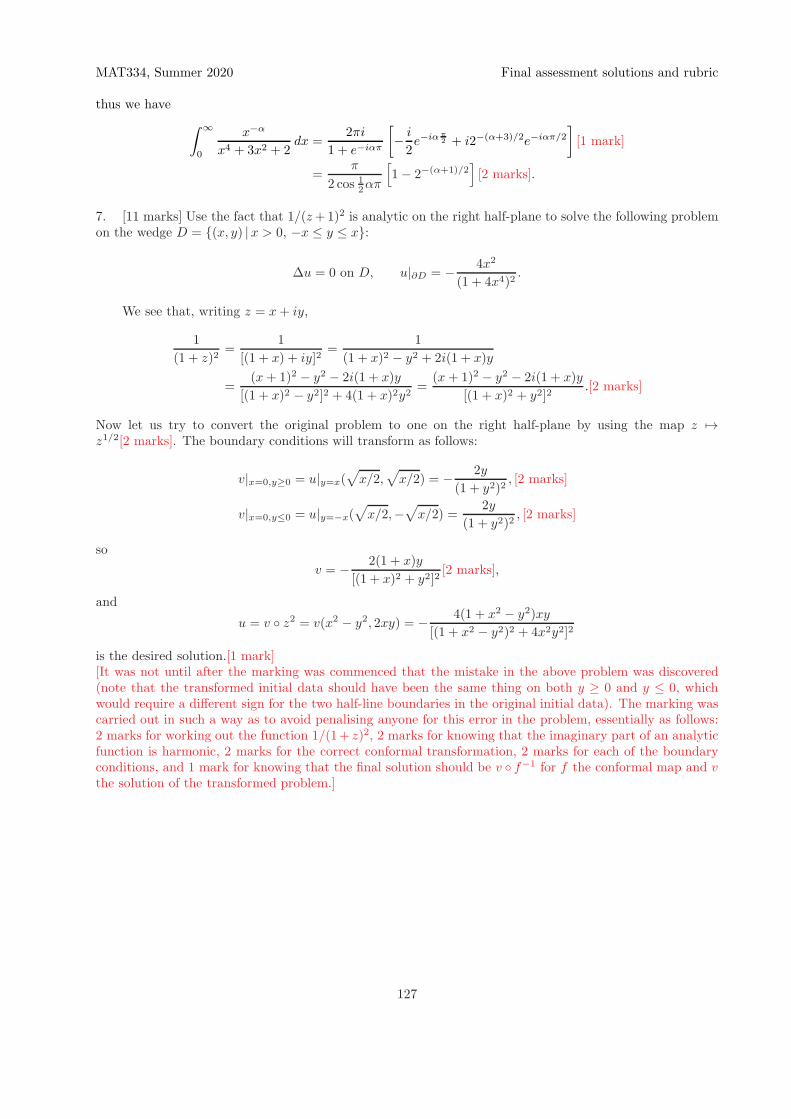
MAT334, Summer 2020 Final assessment solutions and rubric
thus we have
∫ ∞
0
x−α
x4 + 3x2 + 2dx =
2πi
1 + e−iαπ
[
− i
2e−iαπ
2 + i2−(α+3)/2e−iαπ/2
]
[1 mark]
=π
2 cos 12απ
[
1− 2−(α+1)/2]
[2 marks].
7. [11 marks] Use the fact that 1/(z+1)2 is analytic on the right half-plane to solve the following problemon the wedge D = {(x, y) |x > 0, −x ≤ y ≤ x}:
∆u = 0 on D, u|∂D = − 4x2
(1 + 4x4)2.
We see that, writing z = x+ iy,
1
(1 + z)2=
1
[(1 + x) + iy]2=
1
(1 + x)2 − y2 + 2i(1 + x)y
=(x+ 1)2 − y2 − 2i(1 + x)y
[(1 + x)2 − y2]2 + 4(1 + x)2y2=
(x+ 1)2 − y2 − 2i(1 + x)y
[(1 + x)2 + y2]2.[2 marks]
Now let us try to convert the original problem to one on the right half-plane by using the map z 7→z1/2[2 marks]. The boundary conditions will transform as follows:
v|x=0,y≥0 = u|y=x(√
x/2,√
x/2) = − 2y
(1 + y2)2, [2 marks]
v|x=0,y≤0 = u|y=−x(√
x/2,−√
x/2) =2y
(1 + y2)2, [2 marks]
so
v = − 2(1 + x)y
[(1 + x)2 + y2]2[2 marks],
and
u = v ◦ z2 = v(x2 − y2, 2xy) = − 4(1 + x2 − y2)xy
[(1 + x2 − y2)2 + 4x2y2]2
is the desired solution.[1 mark][It was not until after the marking was commenced that the mistake in the above problem was discovered(note that the transformed initial data should have been the same thing on both y ≥ 0 and y ≤ 0, whichwould require a different sign for the two half-line boundaries in the original initial data). The marking wascarried out in such a way as to avoid penalising anyone for this error in the problem, essentially as follows:2 marks for working out the function 1/(1+ z)2, 2 marks for knowing that the imaginary part of an analyticfunction is harmonic, 2 marks for the correct conformal transformation, 2 marks for each of the boundaryconditions, and 1 mark for knowing that the final solution should be v ◦ f−1 for f the conformal map and vthe solution of the transformed problem.]
127
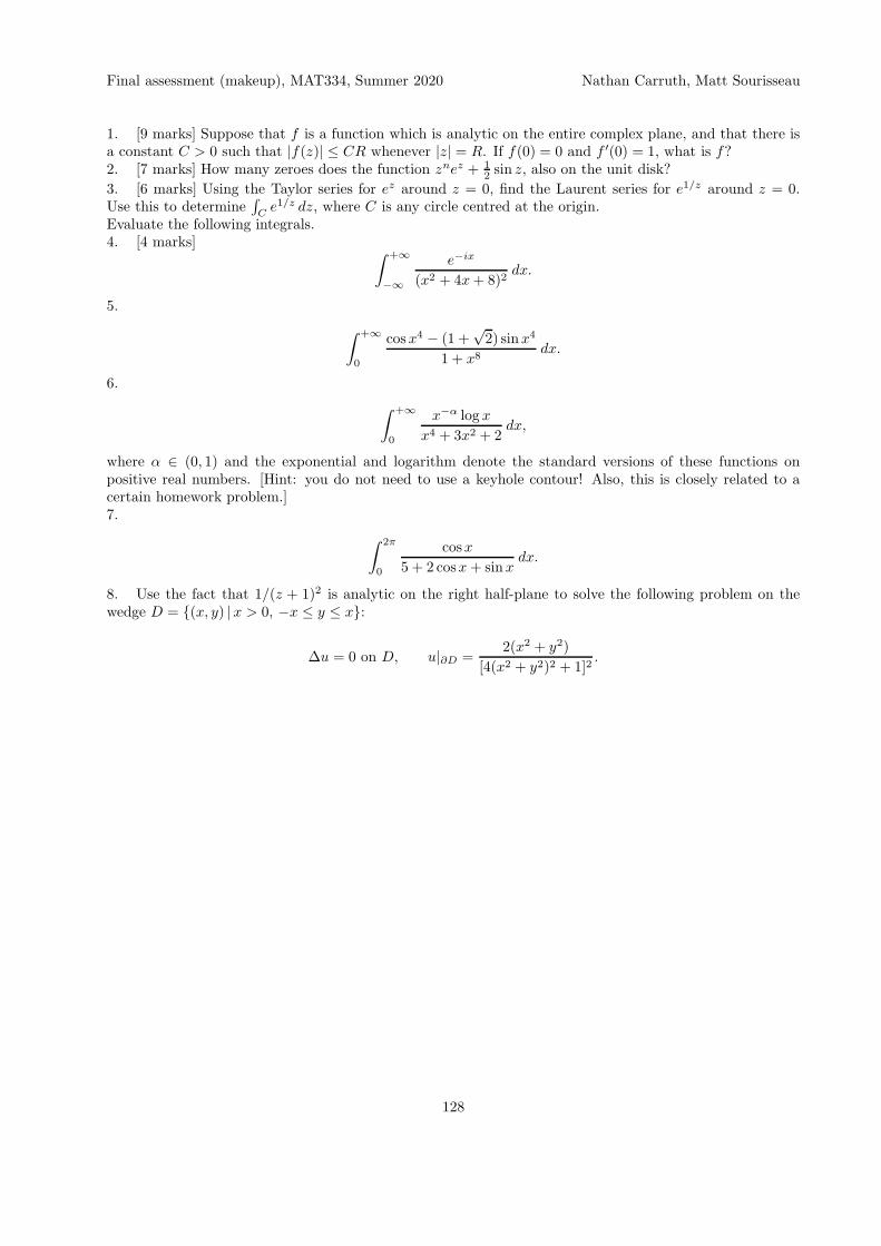
Final assessment (makeup), MAT334, Summer 2020 Nathan Carruth, Matt Sourisseau
1. [9 marks] Suppose that f is a function which is analytic on the entire complex plane, and that there isa constant C > 0 such that |f(z)| ≤ CR whenever |z| = R. If f(0) = 0 and f ′(0) = 1, what is f?2. [7 marks] How many zeroes does the function znez + 1
2 sin z, also on the unit disk?
3. [6 marks] Using the Taylor series for ez around z = 0, find the Laurent series for e1/z around z = 0.Use this to determine
∫
Ce1/z dz, where C is any circle centred at the origin.
Evaluate the following integrals.4. [4 marks]
∫ +∞
−∞
e−ix
(x2 + 4x+ 8)2dx.
5.
∫ +∞
0
cosx4 − (1 +√2) sinx4
1 + x8dx.
6.
∫ +∞
0
x−α log x
x4 + 3x2 + 2dx,
where α ∈ (0, 1) and the exponential and logarithm denote the standard versions of these functions onpositive real numbers. [Hint: you do not need to use a keyhole contour! Also, this is closely related to acertain homework problem.]7.
∫ 2π
0
cosx
5 + 2 cosx+ sinxdx.
8. Use the fact that 1/(z + 1)2 is analytic on the right half-plane to solve the following problem on thewedge D = {(x, y) |x > 0, −x ≤ y ≤ x}:
∆u = 0 on D, u|∂D =2(x2 + y2)
[4(x2 + y2)2 + 1]2.
128

MAT334, 2020. I, §40 [August 6, Supplement] Poisson kernel Nathan Carruth
Summary:
• We motivate the definition of the Poisson kernel.
101. Poisson kernel . In lecture we attempted to give a derivation of the Poisson kernel. While themain idea was correct, there were a few errors in detail and interpretation, and when those are corrected itturns out that what was given can motivate the definition of the Poisson kernel, but does not really serve asa proof. We go through this motivation anyway.
Let D be the disk of radius r centred at the origin, C = ∂D its boundary (the unit circle centred at theorigin), and consider the following problem:
∆u = 0, u|∂D = h, (1)
where ∆ is the Laplacian, ∆u = ∂2u/∂x2 + ∂2u/∂y2, and h is a function on C. Now suppose that there isa function f which is analytic on the complex plane and satisfies Re f |∂D = h; since Re f must be harmoniceverywhere on the plane, and in particular on D, we see that u = Re f is a solution to problem (1). Nowthe Cauchy integral formula allows us to write
f(x+ iy) =1
2πi
∫
C
f(z′)
z′ − [x+ iy]dz′. (2)
If we define
z∗ =r2
z
[note that this corrects an error in the lecture, where z∗ was mistakenly given as r2/z], then z∗ will beoutside of C so that we will have
∫
C
f(x′ + iy′)
z′ − z∗dz′ = 0 (3)
Thus we may subtract this integral from (2). Now we may parameterise C as
z′(t) = reiθ , θ ∈ [0, 2π];
let us write also x+ iy = r0eiθ0 for some θ0. Then (2) becomes, after subtracting (3),
f(x+ iy) =1
2πi
∫ 2
0
π
[
1
reiθ − r0eiθ0− 1
reiθ − r2
r0eiθ0
]
f(reiθ)ireiθ dθ
=1
2π
∫ 2π
0
− r2
r0eiθ0 + r0e
iθ0
(reiθ − r0eiθ0)(
reiθ − r2
r0eiθ0)reiθf(reiθ) dθ
=1
2π
∫ 2π
0
−(r2 − r20)rr0ei(θ0+θ)
(reiθ − r0eiθ0)(
reiθ − r2
r0eiθ0)f(reiθ) dθ
=1
2π
∫ 2π
0
− r2−r20r20
ei(θ0+θ)
(rr0eiθ − eiθ0
)(
eiθ − rr0eiθ0)f(reiθ) dθ
=1
2π
∫ 2π
0
r2−r20r20(
rr0
− ei(θ0−θ))(
rr0
− ei(θ−θ0))f(reiθ) dθ
=1
2π
∫ 2π
0
r2 − r20∣∣r − r0ei(θ0−θ)
∣∣2 f(re
iθ) dθ.
129
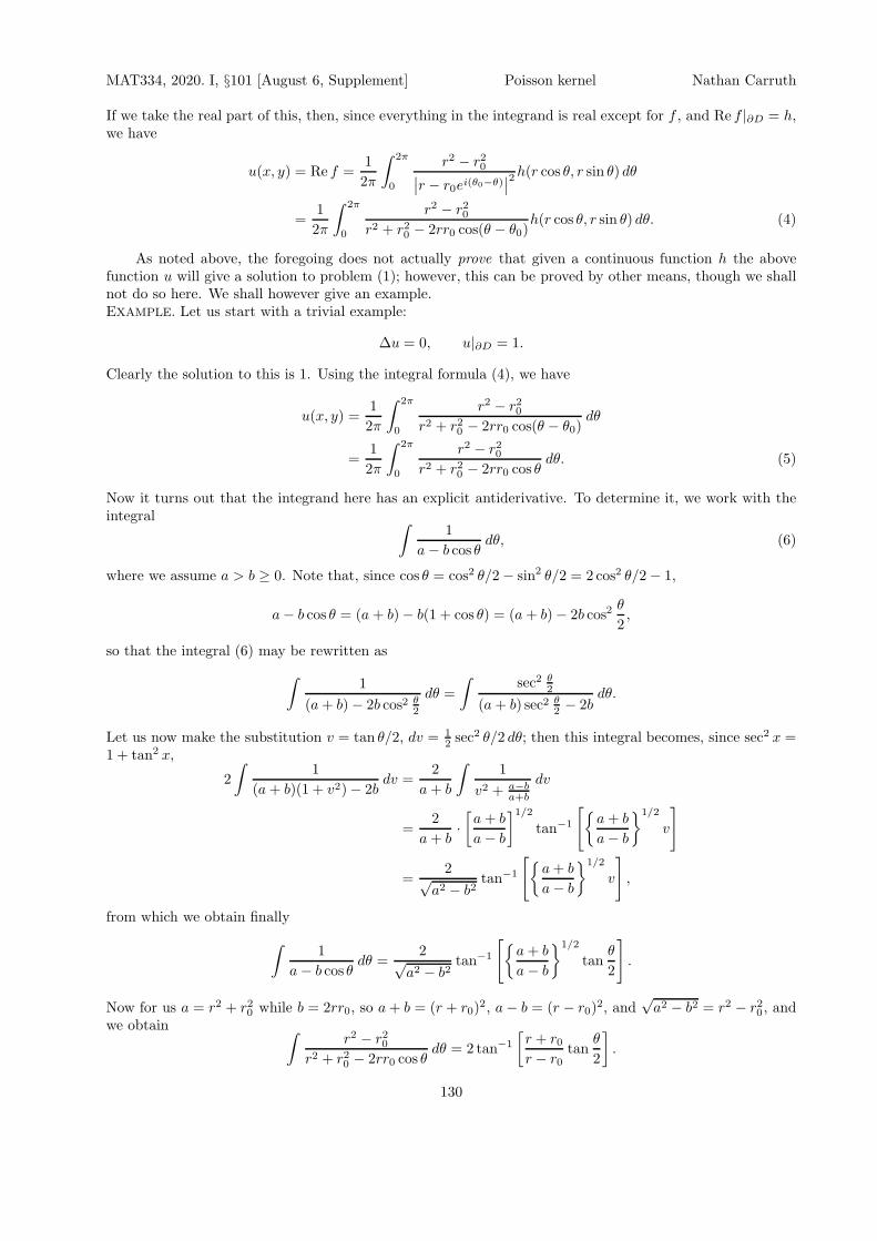
MAT334, 2020. I, §101 [August 6, Supplement] Poisson kernel Nathan Carruth
If we take the real part of this, then, since everything in the integrand is real except for f , and Re f |∂D = h,we have
u(x, y) = Re f =1
2π
∫ 2π
0
r2 − r20∣∣r − r0ei(θ0−θ)
∣∣2h(r cos θ, r sin θ) dθ
=1
2π
∫ 2π
0
r2 − r20r2 + r20 − 2rr0 cos(θ − θ0)
h(r cos θ, r sin θ) dθ. (4)
As noted above, the foregoing does not actually prove that given a continuous function h the abovefunction u will give a solution to problem (1); however, this can be proved by other means, though we shallnot do so here. We shall however give an example.EXAMPLE. Let us start with a trivial example:
∆u = 0, u|∂D = 1.
Clearly the solution to this is 1. Using the integral formula (4), we have
u(x, y) =1
2π
∫ 2π
0
r2 − r20r2 + r20 − 2rr0 cos(θ − θ0)
dθ
=1
2π
∫ 2π
0
r2 − r20r2 + r20 − 2rr0 cos θ
dθ. (5)
Now it turns out that the integrand here has an explicit antiderivative. To determine it, we work with theintegral ∫
1
a− b cos θdθ, (6)
where we assume a > b ≥ 0. Note that, since cos θ = cos2 θ/2− sin2 θ/2 = 2 cos2 θ/2− 1,
a− b cos θ = (a+ b)− b(1 + cos θ) = (a+ b)− 2b cos2θ
2,
so that the integral (6) may be rewritten as
∫1
(a+ b)− 2b cos2 θ2
dθ =
∫sec2 θ
2
(a+ b) sec2 θ2 − 2b
dθ.
Let us now make the substitution v = tan θ/2, dv = 12 sec
2 θ/2 dθ; then this integral becomes, since sec2 x =1 + tan2 x,
2
∫1
(a+ b)(1 + v2)− 2bdv =
2
a+ b
∫1
v2 + a−ba+b
dv
=2
a+ b·[a+ b
a− b
]1/2
tan−1
[{a+ b
a− b
}1/2
v
]
=2√
a2 − b2tan−1
[{a+ b
a− b
}1/2
v
]
,
from which we obtain finally
∫1
a− b cos θdθ =
2√a2 − b2
tan−1
[{a+ b
a− b
}1/2
tanθ
2
]
.
Now for us a = r2 + r20 while b = 2rr0, so a+ b = (r + r0)2, a− b = (r − r0)
2, and√a2 − b2 = r2 − r20 , and
we obtain ∫r2 − r20
r2 + r20 − 2rr0 cos θdθ = 2 tan−1
[r + r0r − r0
tanθ
2
]
.
130
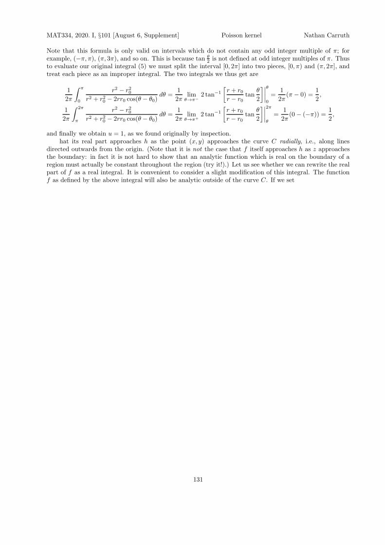
MAT334, 2020. I, §101 [August 6, Supplement] Poisson kernel Nathan Carruth
Note that this formula is only valid on intervals which do not contain any odd integer multiple of π; forexample, (−π, π), (π, 3π), and so on. This is because tan θ
2 is not defined at odd integer multiples of π. Thusto evaluate our original integral (5) we must split the interval [0, 2π] into two pieces, [0, π) and (π, 2π], andtreat each piece as an improper integral. The two integrals we thus get are
1
2π
∫ π
0
r2 − r20r2 + r20 − 2rr0 cos(θ − θ0)
dθ =1
2πlim
θ→π−2 tan−1
[r + r0r − r0
tanθ
2
]∣∣∣∣
θ
0
=1
2π(π − 0) =
1
2,
1
2π
∫ 2π
π
r2 − r20r2 + r20 − 2rr0 cos(θ − θ0)
dθ =1
2πlim
θ→π+2 tan−1
[r + r0r − r0
tanθ
2
]∣∣∣∣
2π
θ
=1
2π(0 − (−π)) = 1
2,
and finally we obtain u = 1, as we found originally by inspection.hat its real part approaches h as the point (x, y) approaches the curve C radially, i.e., along lines
directed outwards from the origin. (Note that it is not the case that f itself approaches h as z approachesthe boundary: in fact it is not hard to show that an analytic function which is real on the boundary of aregion must actually be constant throughout the region (try it!).) Let us see whether we can rewrite the realpart of f as a real integral. It is convenient to consider a slight modification of this integral. The functionf as defined by the above integral will also be analytic outside of the curve C. If we set
131
MAT334, 2020. I, §101 [August 13, Pre-class] An example Nathan Carruth
Summary:• We give a basic introduction to the concept of analytic continuation, and relate it to our discussion ofthe logarithm.102. Analytic continuation. Suppose that we have a function f which is analytic on some region
containing a point a. Since f is analytic near a, we may expand it in a Taylor series near a and write
f(z) =
∞∑
k=0
1
k!f (k)(a)(z − a)k, (1)
and the series will converge to f on the largest disk centred at a on which f is analytic. (A good example tokeep in mind here might be something simple like f(z) = 1/z, expanded around some a 6= 0.) Suppose thatthe series (1) converges on the disk D, necessarily centred at a. Now instead of starting with the functionf , suppose that we instead start with the series (1); in other words, suppose that we simply given a series
∞∑
k=0
ak(z − a)k, (2)
which we know converges on the disk D. Let us denote its sum by f1(z) when z ∈ D (note that we musthave f1(z) = f(z) where f is analytic). Suppose that D has radius r > 0, and let b be a point in D with|b− a| = r− ǫ, where ǫ is small; in other words, b is close to the boundary of D. Now since b ∈ D, the series(2) must converge to an analytic function at b; we may expand thus expand f1 in a Taylor series about band write
f1(z) =
∞∑
k=0
bk(z − b)k. (3)
This series will also converge on a disk, say D′, which must have radius at least ǫ (since the disk of radiusǫ about b will be contained in the disk D by the triangle inequality). However, D′ may have radius biggerthan ǫ; in that case, we say that it gives an extension of the function f1 to the disk D′.
Now clearly there is nothing to keep us from continuing on in this fashion, by taking further points inD or in D′ and expanding the functions around those points to see whether we get further extensions. Atreatment of this is given in Goursat, Chapter IV; sections 83, 84, and 86 in particular are germaine to whatwe shall do here, but we do not have time to go into all of the details and shall content ourselves with aparticular example.
103. A particular example Let us consider the branch of the complex logarithm obtained by takinga cut along the negative real axis and requiring the angle to lie in thet set (−π, π), and denote the resultingbranch by L; in other words, for θ ∈ (−π, π) and r ∈ (0,+∞), we define
L(reiθ) = log r + iθ.
This function is analytic at z = 1, and thus has a power series expansion there – which we shall not give asfinding it is one of the practice problems on the final review sheet; let us denote it by
∞∑
k=0
ak(z − 1)k. (4)
Now this series will converge to L on the largest disk centred at 1 on which L is analytic, which is easilyseen to be the disk of radius 1 centred at z = 1, since L has a singularity at z = 0. Let us call this disk D1.Since L(rei·0) → −∞ as r → 0+, we see that the series (4) cannot converge on any larger disk.
Now let b = 1+i/2; note that b ∈ D1, so the series (4) converges at b. Thus we may expand the resultingfunction about b, obtaining
∞∑
k=0
bk(z − b)k. (5)
132

MAT334, 2020. I, §103 [August 13, Pre-class] An example Nathan Carruth
Now of course on D1 the series (4) converges to L, so we are really just expanding the function L aroundz = b in this case. Thus, once again, the series will converge to L on the largest disk about b which does notinclude any singularity of L; we see that, as above, this will be the disk D2 of radius
√
5/4 about b.Continuing one step further, let us let c = −1/10 + i/2; then |b − c|2 = 112/102 = 121/100 < 5/4, so
c ∈ D2. Thus we may expand the function obtained from the series (5) about z = c, obtaining the series
∞∑
k=0
ck(z − c)k; (6)
as before we are actually expanding the function L, so we know that the series will converge to L on anydisk about c on which L is analytic. This time, though, there is an extra twist. As above, clearly the largest
disk on which the series (6) can converge is the disk, call it D3, of radius |c| =√
51100 about c. However,
clearly the point −1/10 satisfies |c− (−1/10)| = 1/2 <√
51100 ; in other words, −1/10 ∈ D3. But −1/10 was
on the branch cut of L – in other words, the function L is not defined at the point −1/10!Let us investigate what is going on here in more detail. Let L2 denote the branch of Log with a cut
along the negative imaginary axis and with the angle required to lie in (−π/2, 3π/2). Then clearly L = L2
on the fourth, first, and second quadrants (i.e., where θ ∈ (−π/2, π)); thus the series (4) and (5) are also theTaylor series for L2 about z = 1 and z = b, respectively. Similarly, the series (6) is the Taylor series for L2
about z = c, and will converge to L2 on the largest disk about c on which L2 is defined. Now geometricallyit is clear that this disk is indeed the disk D3 – in other words, the series (6) will indeed converge everywhereon D3. It will converge to the function L2 there. Now, as noted, L2 = L for θ ∈ (−π/2, π); but a littlethought shows that L2 − L = 2πi if θ ∈ (π, 3π/2) – they are distinct branches over that interval.
This means, in particular, that for any z = reiθ ∈ D3 with θ ∈ (π, 3π/2), the series in (6) will convergeto a value equal to L(z) + 2πi. Now note that the difference of limits
limθ→π−
L(reiθ)− limθ→−3π/2+
L(reiθ) = 2πi
for any r; in other words, the function L has a jump discontinuity equal to 2πi across the branch cut – itdecreases by 2πi as we cross the branch cut. But this means that if we add 2πi to L as we cross the branchcut, the result will be continuous (as long as we stay close to the branch cut, of course!) – and this is exactlywhat the series (6) accomplishes! In other words, given only local information about the branch L, the serieswas somehow able to pick out the branch L2 which should follow L across the branch cut in order to have afunction which is analytic on both sides of the branch cut.
Now we know of course that there is no branch of the logarithm which is analytic on the entire puncturedplane, so the process of extension given above must run into some irresolvable obstacle at some point. Letus see what that is. Suppose that we continue expanding the function L2 on yet another disk D4 which iscounterclockwisely further around the origin than D3; we are evidently able to do so. If we then continue,using disks say D5, D6, etc., at some point we shall run into the same situation with L2 which we had with L:the series will converge across the branch cut, but to another branch, call it L3, on the other side of the cut,i.e., for θ > 3π/2. As before, we will have L3 − L2 = 2πi for points just across the branch cut; but L2 = Lthere, so L3 − L = 2πi. Now we may take L3 to be the branch with a cut along the positive imaginary axisand the angle θ required to lie in (3π/2, 7π/2). Continuing to expand as before, we will eventually arriveback at the point z = 1. However, at that point we will be expanding the function L3 instead of L, and thatmeans that the series will converge to L3(1) = L(1) + 2πi = 2πi, not L(1) = 0!
Note the close analogy of this procedure to what we discussed much earlier in the course about howintegrating 1/z around the origin to get Log z will increase the value by 2πi – exactly the value determinedhere. The procedure here is however far more general, and in particular could be applied to the rootfunctions, giving the different branches in cyclic succession as we continue expanding around the origin. (Inother words, if we start with one branch of – say – the cube root function, say that which gives 11/3 = 1,and then expand it in Taylor series which circle the origin as here, then when we come back to the point 1again we will have instead e2πi/3; if we circle again, we will have e4πi/3; and if we circle once more – makingthree times in total – we will come back to the original value, 1. With the logarithm, we would continueadding 2πi each time, which means we will never return to the original value no matter how many times we
133
MAT334, 2020. I, §103 [August 13, Pre-class] An example Nathan Carruth
circle.) Similarly, we could apply this to the function in the last problem on the term test: in particular, thelast part shows that if we were to start with the function on one side of the branch cut, and then expand itin series on disks which wrapped around the branch cut to the other side, by the time we came back to theoriginal point there would be a difference of −π/(2
√2).
Those who have seen – or will yet see – covering spaces should note the similarity here to the constructionof the universal cover of the circle, or the punctured plane (which is homotopically equivalent, in fact thereis an obvious deformation retract of the punctured plane onto the circle): we start at a certain point andthen start taking curves, reducing by homotopy; since a closed loop once around the origin is not homotopicto a point, the endpoint of this curve is taken to represent a distinct point from its initial point. Similarly,a closed loop twice about the origin is not homotopic to either of these paths, meaning that its endpointis yet another distinct point, and so on. Another way of putting all of this together is that, should wedefine the logarithm on the universal cover of the punctured plane instead of the punctured plane itself, itwould become a single-valued analytic function. Taking a branch would then correspond to restricting thedomain to some piece of this universal cover for which the covering map is a homeomorphism onto a cutplane. (What we just noted about root functions shows that something similar is true for them, but insteadof needing to use the universal cover of the punctured plane, we need to use, for the nth-root function, then-sheeted cover.) Similarly, functions with more complicated branch points – such as the function on theterm test, which has four branch points; or the arctangent function, which has two – can be defined on coversof the multiply-punctured plane. The fact that if we traverse a loop around all four points we come back tothe same value means however that we do not get the universal cover of the quadruply-punctured plane inthis case, but rather some other set, an elucidation of which is however beyond the knowledge of the presentauthor, who will therefore retire before he says anything more wrong than he already has.
104. A specific example Let us consider the complex logarithm, and try to find its Taylor seriesexpansion about z = 1; in particular, let us see if we can determine what the radius of convergence of thatpower series must be. Immediately there is a problem: shouldn’t we have to specify which branch of thelogarithm we are using? – after all, the logarithm itself is a multivalued function but power series alwaysgive single-valued functions! On the other hand, what do we need to compute the Taylor series of a functionat z = 1? Let us let f denote the ‘logarithm’ (whatever that means in the end, e.g., a particular branch orwhatever we end up deciding on); then what we need is
f(1), f ′(1), f ′′(1), · · · .
Now f(1) will depend on the branch, but since all of the different branches differ by only a constant value,all branches defined at z = 1 will have equal values for the higher derivatives! Moreover, even though f(1)depends on the branch, we still know that no matter which branch we choose, as long as it is defined atz = 1, we will have f(1) = 2nπ for some n ∈ Z. Thus, there is a sequence of numbers a1, a2, · · · such thatfor any branch of Log defined at z = 1, there will be some n ∈ Z such that this branch equals
2nπ +
∞∑
k=1
ak(z − 1)k (7)
(where the sequence ak is given, of course, by
ak =1
k!
dk
dz
k
Log z
∣∣∣∣∣z=1
,
though we are not too interested in this fact right here). Now whether the series (7) converges for a particularvalue of z is clearly independent of the value of n; thus in determining its radius of convergence we may useany branch we like. Now from what we have seen in lecture, the series (7) will converge on the largest diskcentred at z = 1 on which the branch we are dealing with is analytic. Since all branches of the logarithmhave a singularity at the origin, the largest possible radius of convergence for the series (7) is clearly 1. Thatthis is in fact actually its radius of convergence can be seen by taking the branch of the logarithm with a cutalong the negative real axis and an angle required to lie in (−π, π): clearly the origin is the nearest pointon the cut to z = 1, and since this branch will be analytic everywhere else, its Taylor series (7) (here n = 0,
134

MAT334, 2020. I, §104 [August 13, Pre-class] An example Nathan Carruth
but as noted above this is not important) will converge on the disk of radius 1 centred at z = 1, call it D.This is then the same for all other branches of the log function which are defined at z = 1.
But now it seems that we have a problem! Suppose that we take a branch cut along a line radiallyoutwards from the origin and making a very small angle α (positive or negative) with the positive real axis:clearly the resulting function is defined at z = 1, so by the foregoing, its Taylor series at z = 1 must begiven by (7) for some n ∈ Z, and must therefore converge on D. But as long as the angle α is between −π/2and π/2, the branch cut we have chosen will clearly intersect D, meaning that the branch is not analyticeverywhere on D. So evidently we have a case of a Taylor series which converges even across a singularityof the function it is suppose to represent!
With a little more thought, though, this is actually not that confusing. Let us pick some specific numbersto make things concrete. Thus let L1 denote the branch of Log obtained by making a cut along the lineθ = π/4 and requiring the angle to lie in the set (−7π/4, π/4), and let L2 denote the branch of Log obtainedby making a cut instead along the line θ = π/2 and requiring the angle to lie in (−3π/2, π/2). Then clearlyboth of these branches are defined at z = 1, and L1(1) = L2(1) = 0, so that they have the same Taylor series,given by (7) with n = 0. Moreover, if we write out the definitions of these two functions more carefully, wesee that for θ ∈ (−3π/2, π/4) we have
L1(reiθ) = L2(re
iθ) = log r + iθ,
while for θ ∈ (−7π/4,−3π/2) we haveL1(re
iθ) = log r + iθ
but, since the corresponding angle in (−3π/2, π/2) is 2π + θ, we have
L2(reiθ) = log r + i(2π + θ);
in other words, the difference is given by (for θ ∈ (−7π/4, π/4), θ 6= −3π/2)
L1(reiθ)− L2(re
iθ) =
{0, θ ∈ (−3π/2, π/4)
−2πi, θ ∈ (−7π/4,−3π/2).
Now since the branch cut for L2 does not intersect the disk D, the series (7) will not only converge on D,it will actually converge to L2(z) everywhere on D. Thus we can see that the series (7) will converge toL1(z) as long as the argument of z lies between −π/2 and π/4, while it will converge to L1(z) + 2πi if theargument of z is greater than π/4 (in both cases, of course, we assume that z ∈ D as otherwise (7) does notconverge at all).
135

MAT334, 2020. I, §104 [August 11, Supplementary examples] Linear solutions Nathan Carruth
Summary:• We give a more careful treatment of the method of solving Laplace’s equation using linear solutions.105. Linear solutions to boundary value problems for Laplace’s equation. Basically, when
we are solving a boundary-value problem, we are trying to find, by whatever method, a function u whichsatisfies two conditions: (i) it must satisfy Laplace’s equation, i.e., its Laplacian must vanish; (ii) its value onthe boundary of the region must equal the specified function. ‘By whatever method’ means that we do notcare how we obtained the function, only that it satisfies these two conditions; in other words, the methoddoes not need to be constructive or computational in any way. (This is all right since there are generaltheorems which guarantee that the solutions to problems like this are unique, at least when the boundarydata is sufficiently nice.) Obviously, then, one way of ‘finding’ the solution would be to try one functionafter another until (hopefully) the correct one is found. Since there are infinitely many different functionswe might need to try, though, that isn’t a very practical idea. On the other hand, most functions one couldthink of writing down will certainly not satisfy condition (i); for example, sinx certainly doesn’t, nor doessinx sin y, etc.. So maybe a good starting point would be to try to find a collection of functions (ideally allfunctions, though in practice that is again too many) which satisfy Laplace’s equation, and then see if maybewe can somehow find one of them which also has the correct values on the boundary. Now one especiallysimple class of functions which satisfy Laplace’s equation are the linear functions, g(x, y) = a+ bx+ cy: thisis because we can calculate:
∂g
∂x= a,
∂2g
∂x2=
∂
∂xa = 0,
∂g
∂y= b,
∂2g
∂y2=
∂
∂yb = 0,
so
∆g =∂2g
∂x2+∂2g
∂y2= 0.
Now that we know that these functions all satisfy Laplace’s equation, if we are trying to solve a boundary-value problem we only need to find numbers a, b, and c such that the boundary conditions are satisfied. Inother words, we are going to substitute the linear solution a + bx + cy into the boundary conditions in (ii)and try to solve for the numbers a, b, and c. (For anything other than very special boundary conditions,of course, this will not be possible, because the linear solutions are too special; but for the problems onthis assignment this is possible at some point.) Generally we solve for the numbers a, b and c either ‘byinspection’ or by substituting in values for x and y to obtain a system of equations that they must satisfy,which we then try to solve.
Consider the following trivial examples on the unit square D = {(x, y) |x, y ∈ [0, 1]}:EXAMPLE 1. Solve the following problem:
∆u = 0 on D, u|∂D = 1.
If we try a linear solution in this case, then we would say, let us see whether a solution of the formu = a + bx + cy can solve this problem. It clearly solves ∆u = 0; now the condition u|∂D = 1 meansa + bx + cy = 1 whenever (x, y) ∈ ∂D. Thus, for example, if we let x = 1, y = 0 (which is clearly a pointin ∂D), we get a + b = 1; if we let x = 1, y = 1, we get a + b + c = 1, which means c = 0; if we letx = 0, y = 0, we get a = 1, which also means that b = 0 since a + b = 1. Thus the only linear functionwhich could possibly satisfy the boundary conditions is u = 1. But this function clearly does actually satisfythe boundary condition on all of ∂D, and since it satisfies Laplace’s equation (as it had to since it was aparticular example of the class of linear functions, each one of which is a solution to Laplace’s equation), itmust be the desired solution.
EXAMPLE 2. Solve the following problem:
∆u = 0 on D, u|∂D = x.
Let us again try a linear solution: thus we wish to determine whether there are constants a, b, and csuch that u = a+ bx+ cy (which must satisfy Laplace’s equation) satisfies the boundary condition. In thiscase things get a bit more interesting. Suppose that y = 0; then we have, for all x ∈ [0, 1], that a+ bx = x.
136

MAT334, 2020. I, §105 [August 11, Supplementary examples] Linear solutions Nathan Carruth
If we set x = 0, this gives a = 0, so bx = x; if we set x = 1 (or, for that matter, if we let x be any nonzeronumber), this gives b = 1. So far, then, we know that we must have u = x + cy. Now if x = 0 and y 6= 0,say y = 1, then we have by the boundary condition that cy = c = 0. Thus the only linear solution thatcould possibly satisfy the boundary conditions is u = x. Now this does actually clearly satisfy the boundaryconditions; and since it also satisfies Laplace’s equation, it must be the desired solution.
Note however that the solution cannot always be read off from the boundary conditions as in the twoexamples above. For example, the boundary condition in example 2 could have been expressed as follows:u|∂D = 0, x = 0, 1, x = 1, x, y = 0 or y = 1, which we might not immediately recognise – but the methodabove would give u = x as the only solution regardless. For a more involved example, consider the followingproblem:
EXAMPLE 3. Solve the following problem:
∆u = 0 on D, u|∂D =
x, y = 0x+ 1, y = 1y, x = 0
y + 1, x = 1
Let us see whether we can find a linear solution; thus suppose that u = a + bx + cy. The first of theboundary conditions gives a + bx = x for x ∈ [0, 1]; if x = 0 this gives a = 0, while if x = 1 this givesb = 1. Thus we already know that if there is such a solution, it must be of the form u = x + cy. Nowconsider the third of the boundary conditions (u = y when x = 0); this gives cy = y, which, setting y = 1,gives c = 1. Thus the only possible solution would be u = x + y. But now we need to show that this doesindeed satisfy the other two boundary conditions. At y = 1 this expression gives u(x, 1) = x + 1, which isthe correct expression; and at x = 1 it gives u(1, y) = 1 + y = y + 1, which is again the correct expression.Thus u = x + y satisfies the boundary conditions, and since it satisfies Laplace’s equation, it must be thedesired solution.
These are of course rather simple examples, but they demonstrate the technique. More complicatedexamples were given in the lecture notes (see August 11, Section 38, pp. 3 – 4, August 13, Section 40, p. 4);it may be helpful to restudy these in the light of the above explanations.
The same technique is applicable to the problems on the last homework assignment: we posit thatu takes a certain form, and then determine the coefficients by matching that form to the given boundaryconditions.
137

MAT334, 2020. , §105 [May – August] Appendices Nathan Carruth
APPENDIX I. REVIEW OF MULTIVARIABLE CALCULUS AND LINEAR ALGEBRA
I. MULTIVARIABLE CALCULUS
1. Parametric curves. A plane parametric curve1 is a curve in the plane which can be described bytwo equations
x = x(t), y = y(t), (t ∈ [a, b])
for some interval [a, b]; in other words, for every point (x, y) on the curve, there is some value t ∈ [a, b]such that x = x(t) and y = y(t). (Note that this t need not be unique.) More informally, if we view tas a dynamical quantity, the point (x(t), y(t)) ‘traces out’ the entire curve as t varies from a to b. It isoften convenient to represent the point (x(t), y(t)) by a single function, often called γ(t) (the Greek lettergamma), so that γ(t) = (x(t), y(t)). We shall use γ (without t) to refer to the entire curve, considered asa single object. When necessary to distinguish between the function γ(t) and the plane curve this functionrepresents, we shall call the latter the image of γ.
A curve is called closed when (in the notation of the previous paragraph) γ(a) = γ(b). A closed curvewhich does not intersect itself (i.e., for which the value of t mentioned above is unique) is called a Jordancurve. A Jordan curve γ is said to be oriented counterclockwise if, as t increases from a to b, the point γ(t)traces out the curve in a counterclockwise direction, and similarly to be oriented clockwise if this point tracesout the curve in a clockwise direction.2 We note for future use that if D is a connected region of the plane,then its boundary curve is always a Jordan curve. This result has a converse in the so-called Jordan curvetheorem which we shall mention later on in the course.
General parametric curves can display pathological behaviour, even when x(t) and y(t) are both con-tinuous.3 In this course we shall deal exclusively with so-called piecewise-smooth curves, defined as follows.A parametric curve γ is said to be piecewise-smooth on an interval [a, b] if (i) it is continuous on [a, b] and(ii) there are points t0 = a < t1 < · · · < tn = b such that on each subinterval (ti, ti+1), i = 0, · · · , n − 1,the derivative γ′(t) = x′(t)i + y′(t)j4 exists, and is continuous and nonzero. (Condition (ii) amounts tosaying that x(t) and y(t) are continuously differentiable on (ti, ti+1), and that x′(t) and y′(t) never vanishsimultaneously. This last requirement is necessary to avoid ‘corners’; see the practice problems!)
A piecewise smooth curve has a well-defined length. Recall that the length of a parametric curve γdefined on some interval [a, b] and such that γ′ is continuous there is given by
∫ b
a
|γ′(t)| dt,
where | · | denotes the length of a vector. This definition can be extended to a piecewise-smooth curve in anobvious way: if t0, t1, . . . , tn are the points given in the definition of piecewise-smoothness, then we definethe length of γ to be5
∫ t1
t0
|γ′(t)| dt+∫ t2
t1
|γ′(t)| dt+ · · ·+∫ tn
tn−1
|γ′(t)| dt =n−1∑
i=0
∫ ti+1
ti
|γ′(t)| dt.
1 Parametric curves can, of course, also be considered in three (and even arbitrary) dimensions. In thiscourse, though, we shall only need them in two.
2 Note that this definition would not make sense for a self-intersecting curve: for example, no matter howyou trace out a figure-eight, the upper part will be oriented one way while the lower part will be orientedanother.
3 For example, one can find a parametric curve which – at least if we are allowed to replace the boundedinterval [a, b] by the whole real line – essentially fill out an entire two-dimensional region!
4 While we shall not need to make this distinction in this course, it bears pointing out that, technicallyspeaking, points and vectors are not identical, and when one must distinguish between them, a curve γ givesa point for each t while its derivative gives a vector.
5 To be precise, the integrals here should be understood as improper integrals obtained by integratingfrom something slightly greater than ti to something slightly less than ti+1, and then taking the limit asthese endpoints approach those two values, respectively; but this is generally not something which needs tobe made explicit in practice, and we shall generally pass over it in silence in similar cases in the future.
138
MAT334, 2020. , §105 [May – August] Appendices Nathan Carruth
The main use we shall make of parametric curves is in line integrals (see §3 below), and also in describinghow two points in the plane are connected. This latter will become clearer as we progress through the course.The fact that two real numbers are essentially only connected in one way, while two complex numbers canbe connected in multiple ways, some of which may be distinct (in an appropriate sense), is part of whatmakes complex analysis interesting.
2. Partial derivatives. Suppose that we have a function f defined on a region of the plane, whichwe suppose has Cartesian coordinates (x, y). We define its partial derivatives with respect to x and y to be
∂f
∂x= lim
h→0
f(x+ h, y)− f(x, y)
h,
∂f
∂y= lim
h→0
(f(x, y + h)− f(x, y)
h.
We recall that in multivariable calculus we saw that the existence of both partial derivatives still allowed forquite a bit of pathological behaviour. It turns out that for functions of a complex variable there are additionalrequirements on the partial derivatives in order for the function to have a single complex derivative, andthat these requirements, though simple, lead to far-reaching results which rule out all such pathologicalbehaviours.
Recall that if a function f has a local extremum at a point where its partial derivatives exist, then theymust both vanish.
Some examples of partial derivatives are given in the review problems.[This paragraph is an aside for students who have had MAT237 or MAT257, or who have otherwise
learned how to view the derivative as a linear map. In this class we shall be interested in complex-valuedfunctions of a complex variable; since the set of complex numbers is a two-dimensional vector space over thereal numbers, this means that we are in essence considering functions from R2 to R2 (or, in essence, a vectorfield on R2). Thus the derivative of such a function, in the multivariable-calculus sense, should be a linearmap from R2 to R2 approximating the original function at the point of differentiation. It turns out that therequirement that a complex derivative exists requires that this map be a composition of an isotropic scaling(i.e., multiplication by a single real number) and a rotation. This is the basis for the study of functions of acomplex variable as conformal maps, namely functions from R2 to R2 which preserve angles.]
3. Line integrals and vector fields. Suppose that γ is a piecewise-smooth curve on an interval[a, b] (γ(t) = (x(t), y(t))), and that f is a continuous function defined on some set containing the image of γ.Then we define three different types of line integral along γ, as follows. Let t0, t1, · · · , tn be the points givenin the definition of piecewise-smoothness; then we define
∫
γ
f dx =n−1∑
i=0
∫ ti+1
ti
f(x(t), y(t))x′(t) dt
∫
γ
f dy =n−1∑
i=0
∫ ti+1
ti
f(x(t), y(t)) y′(t) dt
∫
γ
f ds =n−1∑
i=0
∫ ti+1
ti
f(x(t), y(t)) |γ′(t)| dt,
and call these the line integrals of f along γ with respect to x, y, and arclength, respectively.Recall that a vector field on a region of R2 is a function which to every point in its domain associates
a vector in R2; in other words, it can be written as a function F(x, y) = P (x, y)i +Q(x, y)j, where P (x, y)and Q(x, y) are functions defined on the region called (naturally) the components of the vector field. If thevector field F is defined on a region containing γ, then we may combine the line integrals with respect to xand y of the components of F to define a new line integral, as follows:
∫
γ
P (x, y) dx+
∫
γ
Q(x, y) dy =
∫
γ
F(x, y) · dx.
139

MAT334, 2020. , §105 [May – August] Appendices Nathan Carruth
We call this the line integral of the vector field along the curve γ. Recall the following fundamental theoremof calculus for line integrals: If F = ∇f for some function f , i.e., if F is a gradient, then
∫
γ
F · dx = f(γ(b))− f(γ(a)),
and this integral is therefore independent of the choice of path γ. This notion of path-independence (thisis a standard term, though in our current setting it would be more natural to call it curve-independence!),namely that the line integral along a certain curve only depends on the end-points of the curve and not onthe curve itself, is of central importance in the study of analytic functions of a complex variable. Recallthat it is equivalent to the requirement that the line integral along any closed curve be zero. This is in turnrelated to Green’s theorem, which states that for any vector field F = P (x, y)i + Q(x, y)j and any closedcurve γ bounding a connected region D and oriented counterclockwise,
∫
γ
F · dx =
∫∫
D
(∂Q
∂x− ∂P
∂y
)
dA,
where the latter is an area integral over the region D. This is a special case of Stokes’s theorem, whichwe shall not need in its full generality but which we state here because it provides useful notation: If Sis any (sufficiently smooth) connected surface in R3 with boundary curve C, and S and C are orientedconsistently,6 then ∫
C
F · dx =
∫∫
S
curlF · n dA.
Here the second integral is a surface integral and n represents the unit normal to the surface S, but we shallnot need these things in this class. The curl of a vector field can be defined heuristically as curlF = ∇×F;if F is a vector field on R2 then the curl can be taken to be the single number
∂Q
∂x− ∂P
∂y
appearing in Green’s theorem. For us this is the only case for which we shall need to use the curl (and weshall not need to use it much even here).
Note now that Green’s theorem tells us that line integrals of a vector field are path-independent exactlywhen the curl of that vector field is zero. Such a vector field is called conservative, though we shall onlyneed this term only occasionally. We have seen that a vector field which is the gradient of a function isconservative; on a so-called simply connected region – by which we mean a region ‘without holes’, or, moreprecisely, whose boundary is a single Jordan curve – the converse is also true. We shall see that these resultshave analogues in the theory of functions of a complex variable, though the results generally are not quiteexact copies.
II. LINEAR ALGEBRA
4. Matrices. In this course we shall not need much from the results of linear algebra, but mostly afamiliarity with its concepts. Recall that a matrix of size m by n is a two-dimensional array of numbers
[aij ] =
a11 a12 · · · a1na21 a22 · · · a2n...
.... . .
...am1 am2 · · · amn
,
and is called square if m = n. The product of matrices [aij ] and [bjk] of sizes m by n and n by ℓ is definedto be the matrix [cik] of size m by ℓ given by
cik =
n∑
j=1
aijbjk.
6 For us, this just means that were γ oriented clockwise we would need to introduce an extra minus signon the right-hand side of Green’s theorem.
140

MAT334, 2020. , §105 [May – August] Appendices Nathan Carruth
Recall that the identity matrix of size n by n
I =
1 0 0 · · · 00 1 0 · · · 0...
......
. . ....
0 0 0 · · · 1
has the property that AI = A and IB = B for any matrices A and B of size m by n and n by ℓ, respectively.If a matrix A = [aij ] is square of size n by n, then its inverse (when it exists) is a matrix A−1 of size n byn satisfying
AA−1 = A−1A = I.
In general, finding an inverse matrix is hard. For two-by-two matrices, however, there is a simple formulawhich is often useful, given by Cramer’s rule: If
A =
[a bc d
]
,
then
A−1 =1
ad− bc
[d −b−c a
]
,
as long as ad − bc 6= 0. The quantity ad − bc is called the determinant of the matrix A; the notion ofdeterminant can be defined for a square matrix of any size, but as the general definition is complicated andwe shall not need it in this course we pass over it for the moment.
Recall that a matrix of size m by n can be viewed as giving a linear transformation from Rn to Rm.In particular, a 2 by 2 matrix can be viewed as a linear transformation on the plane. Two particularlyimportant and simple examples are isotropic scaling and rotation. The first is just multiplication by a singlescalar and corresponds to the matrix (λ 6= 0)
[λ 00 λ
]
, which has inverse
[λ−1 00 λ−1
]
.
The second is a bit more complicated. Consider rotation of the plane by an angle θ counterclockwise aroundthe origin. Since vector addition and scalar multiplication in the plane can be defined in terms of geometricpictures which are transformed rigidly by such a rotation, we see that this rotation must be linear; thusit suffices to determine its effect on the basis vectors i and j of the plane. If we rotate the vector i byan angle θ counterclockwise around the origin, a little geometry makes it clear that we obtain the vectorcos θi+sin θj, while if we rotate j the same way we obtain the vector − sin θi+cos θj; thus the matrix givingthis transformation is [
cos θ − sin θsin θ cos θ
]
.
We note two interesting properties of this matrix: first, its determinant is
cos θ · cos θ − (− sin θ) · sin θ = cos2 θ + sin2 θ = 1;
secondly, its inverse is (by the general formula above)
[cos θ sin θ− sin θ cos θ
]
,
which is just the original matrix with θ replaced by −θ! This makes good sense since the inverse to acounterclockwise rotation by θ is a clockwise rotation by θ, which is essentially just a counterclockwiserotation by −θ.
141

MAT334, 2020. , §105 [May – August] Appendices Nathan Carruth
APPENDIX II. BASIC DEFINITIONS AND PROPERTIES OF COMPLEX NUMBERS.
1. Basic definitions. A complex number is an abstract quantity z = a + ib, where a and b are realnumbers and i is an abstract quantity which we require to satisfy i2 = −1.1 We require that these numberssatisfy all of the usual properties of arithmetic; thus if z1 = a1 + ib1 and z2 = a2 + ib2, we have
z1 + z2 = (a1 + a2) + i(b1 + b2)
z1 · z2 = a1a2 − b1b2 + i(a1b2 + b1a2.
We define the conjugate of a complex number z = a+ ib to be the complex number
z = a− ib,
and note that the productzz = a2 + b2
is always real and nonnegative. By the Pythagorean theorem,√zz is the distance from the origin to the
point (a, b), and we call this quantity the modulus2 (or, sometimes, the absolute value or even the length) ofthe complex number z, and denote it as
|z| =√zz.
The function | · | satisfies all of the usual properties of the absolute value function on real numbers:
|z1z2| = |z1||z2|, |z1 + z2| ≤ |z1|+ |z2|.
Since geometrically | · | represents distance from the origin, a set of the form
{z||z − z0| < R}
is a circle of radius R centred at the point corresponding to z0.The ratio of two complex numbers can be determined as follows. Let z1 = a+ ib, z2 = c+ id be complex
numbers with z2 6= 0; thenz1z2
=z1z2z2z2
=(a+ ib)(c− id)
c2 + d2
=ac+ bd
c2 + d2+ i
bc− ad
c2 + d2.
Let z = a+ ib be a complex number, and consider the corresponding point (a, b) in the plane. Let thispoint have a polar representation (r, θ), where r is the distance to it from the origin and θ is the angle fromthe positive x axis to a ray from the origin to the point, measured counterclockwise. Then we may write
a = r cos θ, b = r sin θ,
so that we havez = r(cos θ + i sin θ).
Here, clearly, r = |z|. The angle θ is called the argument of the complex number z and is defined onlyup to a multiple of 2π. From the definition of the complex exponential below it follows that we may writeequivalently
z = reiθ .
If z1 = r1eiθ1 and z2 = r2e
iθ2 are any two complex numbers, then it is not hard to show that their producthas the polar representation
z1z2 = r1r2ei(θ1+θ2),
1 For those who are familiar with fields, we note that we may view the set of complex numbers as thequotient field R[x]/(x2 + 1), which is quite natural since we wish it to be the real field R with a root of theequation x2 + 1 = 0 attached. In this quotient field the equivalence class of x plays the role of i.
2 Plural, moduli.
142
MAT334, 2020. , §105 [May – August] Appendices Nathan Carruth
i.e., that moduli multiply while arguments add. Geometrically, multiplying complex numbers amounts tomultiplying lengths and adding angles. Further,
z1z2
=r1r2ei(θ1−θ2),
i.e., dividing corresponds to dividing lengths and subtracting angles. If m is any positive integer, then, wehave
zm = z · z · · · z︸ ︷︷ ︸
m times
= rmeimθ.
If m is a negative integer, we define
zm =1
z|m| ,
and it is simple to show that in this case also
zm = rmeimθ,
i.e., that this formula holds for all nonzero integer exponents m. For nonzero z we define z0 = 1, and thisformula then holds for all integer exponents.
143