Faculty of Science and Technology

MASTER’STHESIS

Study program/ Specialization:

Computer Science

Spring semester, 2015

Open / Restricted access

Writer:

Chengwei Xiao

…………………………………………

(Writer’s signature)

Faculty supervisor:

Dr. Rui Máximo Esteves, Prof. Chunming Rong

Title of thesis:

Using Machine Learning for Exploratory Data Analysis and Predictive

Models on Large Datasets

Credits (ECTS):

30

Key words:

Machine Learning

Exploratory Data Analysis

Regression Model

Ordinary Linear Regression

Artificial Neural Networks

Random Forest

Pages: …………………

+ enclosure: …………

Stavanger, ………………..

Date/year

UNIVERSITY OF STAVANGER

MASTER OF COMPUTER SCIENCE

USING MACHINE LEARNING FOR EXPLORATORY DATA

ANALYSIS AND PREDICTIVE MODELS ON LARGE

DATASETS

by

CHENGWEI XIAO

Department of Electrical Engineering and Computer Science

Faculty of Science and Technology

June 2015

Approved by:

Dr. Rui Máximo Esteves Prof. Chunming Rong

i

Acknowledgements

First of all, I would like to express the heartfelt thanks to my supervisors, Prof. Chunming

Rong and Dr. Rui Esteves. The investigation of the research direction, the working-out of the

research process and the achievements of the paper have all benefited from their strong support

and elaborate guidance. No matter in scientific research or in life, their valuable advice and

suggestions can always make me enlightened and feel relieved. At the moment of the completion

of the master thesis, I honor both of you sincerely.

In addition, I would also like to thanks my “Madla” friends who give me a lot of help and

support during the two years’ study life at University of Stavanger in Norway, they are：Jiaqi

Ye, Long Cui, Wei Liao, Dongjing Liu, Shuo Zhang, Guoqin Sun, Pengyu Zhu, Jia Geng,

Xiaoan Zhong, Zhichao Li, Weijie Liu, Hao Li, Ting Xu, Jing Hou and so on. I am very glad to

be acquainted with them, and it is them who make this IT-guy not lonesome in a foreign country.

Thanks all my friends for giving me such a wonderful and meaningful two years’ study life here

in Stavanger.

Last but not least, thanks to my beloved parents, whose good care and quiet support is the

driving force for my successful completion of the master study!

ii

Abstract

With the advent of the era of big data, machine learning has been widely used in many

technologies and industries, which is able to get computers to learn without being explicitly

programmed. As one of the fields of the supervised learning, some classical types of regression

models, including the linear regression, nonlinear regression and regression trees, are discussed

at first. And some representative algorithms in each category and their advantages and

disadvantages are also illustrated as well. After that, the data pre-processing and resampling

techniques, including data transformation, dimensionality reduction and k-fold cross-validation,

are explained which can be used to improve the performance of the training model. During the

implementation of machine learning algorithms, three typical models (Ordinary Linear

Regression, Artificial Neural Networks and Random Forest) have been implemented by the

different packages in R on the given large datasets. Apart from the model training, the regression

diagnostics are conducted to explain the poorly predictive ability of the simplest ordinary linear

regression model. Due to the non-deterministic feature of the artificial neural network and

random forest models, several small models are built on small number of samples in the dataset

to get the reasonable tuning parameters, and the optimal models are chosen by the value of

RMSE and R2 among several training models. The corresponding performance of the built

models are quantitatively and visually evaluated in details.

The quantitative and visual results of our practical implementation show the feasibility for

the large datasets under the artificial neural network and random forest algorithms. Comparing

with the ordinary linear regression model (RMSE = 65556.95, R2 = 0.7327), the performance of

the artificial neural network (RMSE = 36945.95, R2 = 0.9151) and random forest (RMSE =

30705.78, R2 = 0.9417) models are greatly improved, but the model training process is more

complex and more time-consuming. The right choice between different models relies on the

characteristics of the dataset and the goal, and also depends upon the cross-validation technique

and the quantitative evaluation of the models.

Keywords: Machine Learning, Exploratory Data Analysis, Regression Model, Ordinary Linear

Regression, Artificial Neural Networks, Random Forest

iii

Table of Contents

Acknowledgements .......................................................................................................................... i 

Abstract ........................................................................................................................................... ii 

Table of Contents ........................................................................................................................... iii 

List of Figures ................................................................................................................................ vi 

List of Tables ............................................................................................................................... viii 

Chapter 1 - Introduction .................................................................................................................. 1 

1.1 Machine Learning ................................................................................................................. 1 

1.2 Development of Machine Learning ...................................................................................... 2 

1.3 Types of Machine Learning Algorithms ............................................................................... 4 

1.3.1 Supervised Learning ...................................................................................................... 4 

1.3.2 Unsupervised Learning .................................................................................................. 5 

1.4 Thesis Organization .............................................................................................................. 5 

Chapter 2 - Regression Models ....................................................................................................... 7 

2.1 Linear Regression ................................................................................................................. 7 

2.1.1 Ordinary Linear Regression ........................................................................................... 8 

2.1.2 Partial Least Squares ...................................................................................................... 9 

2.1.3 Penalized Regression Models ...................................................................................... 10 

2.2 Nonlinear Regression .......................................................................................................... 12 

2.2.1 Multivariate Adaptive Regression Splines ................................................................... 12 

2.2.2 Support Vector Machines ............................................................................................ 14 

2.2.3 Artificial Neural Networks........................................................................................... 16 

2.2.4 K-Nearest Neighbors ................................................................................................... 18 

2.3 Regression Trees and Related Models ................................................................................ 19 

2.3.1 Basic Regression Tree .................................................................................................. 19 

2.3.2 Bagging Tree ................................................................................................................ 21 

2.3.3 Random Forest ............................................................................................................. 22 

2.3.4 Boosted Tree ................................................................................................................ 23 

2.4 Summary ............................................................................................................................. 26 

Chapter 3 - Data Pre-processing and Resampling Techniques ..................................................... 27 

iv

3.1 Data Transformation ........................................................................................................... 27 

3.1.1 Adding or Deleting Variables ...................................................................................... 27 

3.1.2 Centering and Scaling .................................................................................................. 28 

3.1.3 Transforming Variables ............................................................................................... 28 

3.2 Dimensionality Reduction .................................................................................................. 29 

3.2.1 Feature Selection .......................................................................................................... 29 

3.2.2 Feature Extraction ........................................................................................................ 30 

3.2.3 Principal Components Analysis ................................................................................... 31 

3.3 k-Fold Cross-Validation ..................................................................................................... 32 

3.4 Summary ............................................................................................................................. 33 

Chapter 4 - Implementation of Machine Learning Algorithms .................................................... 34 

4.1 Overview of the Dataset ..................................................................................................... 34 

4.2 Data Pre-processing in R .................................................................................................... 35 

4.2.1 Filtering the Variables .................................................................................................. 35 

4.2.2 Transformations ........................................................................................................... 38 

4.2.3 PCA vs PLS ................................................................................................................. 38 

4.2.4 Data Splitting ............................................................................................................... 43 

4.3 Ordinary Linear Regression ................................................................................................ 45 

4.3.1 Multiple Linear Regression .......................................................................................... 45 

4.3.2 Measuring Performance in OLR Model ...................................................................... 46 

4.3.3 Regression Diagnostics ................................................................................................ 48 

4.4 Artificial Neural Networks ................................................................................................. 50 

4.4.1 Choosing Tuning Parameters ....................................................................................... 50 

4.4.2 Building ANN Model .................................................................................................. 53 

4.4.3 Measuring Performance in ANN Model ...................................................................... 54 

4.5 Random Forest .................................................................................................................... 57 

4.5.1 Choosing Tuning Parameters ....................................................................................... 57 

4.5.2 Building RF Model ...................................................................................................... 59 

4.5.3 Measuring Performance in RF Model .......................................................................... 60 

4.6 Summary ............................................................................................................................. 64 

Chapter 5 - Conclusions ................................................................................................................ 65 

v

Appendix – Source Code .............................................................................................................. 69 

Data Pre-processing .................................................................................................................. 69 

Ordinary Linear Regression ...................................................................................................... 72 

Artificial Neural Networks ....................................................................................................... 73 

Random Forest .......................................................................................................................... 78 

vi

List of Figures

Figure 2.1 Main Structure of a PLS Model .................................................................................. 10 

Figure 2.2 Diagram of a Typical Artificial Neural Network ....................................................... 16 

Figure 2.3 K-Nearest Neighbors with K=3 and K=7 ................................................................... 18 

Figure 2.4 Example of Bagging Tree ........................................................................................... 21 

Figure 2.5 a General Random Forests Algorithm [25] ................................................................ 22 

Figure 2.6 a Simple Gradient Boosting Algorithm ...................................................................... 25 

Figure 3.1 an Example of 3-Fold Cross-Validation [25] ............................................................. 32 

Figure 4.1 Correlogram of Variables without Near Zero Variance ............................................. 37 

Figure 4.2 Results of the Dataset Transformations ...................................................................... 38 

Figure 4.3 Scree Plot with Parallel Analysis ............................................................................... 39 

Figure 4.4 Principal Components Analysis without Rotation ..................................................... 40 

Figure 4.5 Principal Components Analysis with Rotation ........................................................... 41 

Figure 4.6 Cross-validated RMSEP and R2 by Components for PLSR and PCR ....................... 43 

Figure 4.7 Summary of the Outcome Variable in the Training Set and Testing Set ................... 44 

Figure 4.8 Multiple Linear Regression Model ............................................................................. 45 

Figure 4.9 10-fold Cross-validated R2 ......................................................................................... 46 

Figure 4.10 Calculations of the RMSE and R2 Values ................................................................ 47 

Figure 4.11 Visualizations of the Linear Regression Model Fit .................................................. 48 

Figure 4.12 Diagnostic Plots for Multiple Linear Regression Model .......................................... 49 

Figure 4.13 train() Function for Choosing ANN Tuning Parameters ......................................... 51 

Figure 4.14 RMSE Profiles for ANN model by train() function ................................................. 52 

Figure 4.15 Artificial Neural Network Model ............................................................................. 53 

Figure 4.16 Summary of the ANN Model ................................................................................... 54 

Figure 4.17 Source Code for Quantitative Results of ANN model .............................................. 55 

Figure 4.18 Visualizations of the ANN Model Fit ...................................................................... 56 

Figure 4.19 train() Function for Choosing RF Tuning Parameters ............................................. 57 

Figure 4.20 RMSE Profiles for RF model by train() function .................................................... 58 

Figure 4.21 Random Forest Model .............................................................................................. 59 

vii

Figure 4.22 Summary of the Random Forest Model ................................................................... 60 

Figure 4.23 Visualizations of the RF Model Fit .......................................................................... 61 

Figure 4.24 Variable Importance Scores for the 15 Predictors in the RF Model ........................ 62 

Figure 4.25 Dot-chart of Variable Importance Scores ................................................................. 63 

Figure 4.26 Histogram of Tree size for the RF Model ................................................................ 63 

viii

List of Tables

Table 3.1 Common Transformation Functions ............................................................................ 29 

Table 4.1 Resume of the Datasets ................................................................................................ 34 

Table 4.2 Optimal Results of the train() Function ....................................................................... 52 

Table 4.3 Quantitative Results of ANN Models by the nnet() Function ..................................... 55 

Table 4.4 Optimal Results of the train() Function ....................................................................... 58 

Table 4.5 Quantitative Results of RF Models by the randomForest() Function ......................... 60 

1

Chapter 1 - Introduction

With the advent of the era of big data, Big Data is becoming a central issue for academia

and industry. It has been widely used in many technologies and industries, from a search engine

to the recommendation system for understanding and targeting customers; from the large-scale

databases to data mining applications for optimizing machine and device performance; from

scientific research to business intelligence for understanding and optimizing business

processes … many aspects of our lives have been affected and made a real big difference today.

However, due to the features of big data, such as complexity, high-dimensionality, frequent-

variability, it is difficult to automatically reveal knowledge and useful information from real,

unstructured and complicated large datasets. Thus, there is an urgent need for applying machine

learning to big data.

1.1 Machine Learning

Machine Learning is an interdisciplinary filed, involving probability theory, statistics,

computational complexity theory, approximation theory and many other computer science

subjects. It is the study of computer simulation or realization of human being behavior so as to

acquire new knowledge or skills, and recognizing the existing knowledge structures to

continuously improve their performance. As the core of artificial intelligence, it is a fundamental

way to make computers intelligent by summarizing and synthesizing in various areas of its

applications [1, 2].

Learning ability is a significant feature of intelligent behavior, but so far it is still not clear

about the mechanism of learning process. There are various definitions of machine learning, for

instance, H. A. Simon believes that learning is adaptive changes made to a system, making the

system more effective to complete the same or similar tasks [3]. R. S. Michalski argues that

learning is to construct or modify representation for experienced things [4-6]. Professionals

engaged in the development of learning systems believe that learning is the acquisition of

knowledge [7-9]. These views have different emphasis, the first one focused on the effect of the

external behavior, and the second emphasizes the internal processes of learning, and the third

mainly from the practical point of knowledge engineering.

2

In mathematics, the machine learning method can be defined as [10]: suppose that in a

computer program, for a class of task T, which can be measured its performance by P, it requires

experience E to improve, this program can be named as learning from experience E, for the task

T, measured its performance by P. There are three main characteristics of the precise definition

to be identified in machine learning: type of task T, experience E, and the specific criteria for the

improvement of task P.

Machine learning has an essential position in the study of artificial intelligence. It is

difficult to claim a system to be truly intelligent if it does not have the ability to learn, but

intelligent systems in the past have generally lack the ability to learn. For example, they cannot

be self-correcting an error, cannot improve their performance through experience, cannot

automatically get and discovery the required knowledge. They are limited to deductive reasoning

and lack of induction. Therefore, at most only able to prove the existing facts and theorems, but

cannot discover new theorems, laws and rules. With the development of artificial intelligence,

these limitations become more prominent. It is under such circumstance that machine learning

gradually become the core of artificial intelligence research. Its applications have become

popular in various subfields of artificial intelligence, such as expert systems, automated

reasoning, natural language understanding, pattern recognition, computer vision, intelligent

robotics [5, 11].

Research in machine learning is based on physiology, cognitive science, etc. to understand

the mechanism of human learning ability [5, 12]. The cognition models or computational models

of human learning process are built, a variety of learning theory and learning approaches are

developed, the general learning algorithms are studied, and the theoretical analysis is done. After

that, a learning system with specific task-oriented applications is built. These research objectives

always have a reciprocal impact, progress in one sector promoting progress in the other.

1.2 Development of Machine Learning

As early as in ancient times, the human mind conceived the idea of intelligent machines.

About 4500 years ago, the South Pointing Chariots were invented in China, and the well-known

ancient Chinese wooden walking horses invented by Zhuge Liang during the Three Kingdoms

period. Japanese made the dolls driven by a mechanical device hundreds of years ago. These

examples are just an understanding and attempt of machine learning for the early human.

3

The real machine learning research started late, and its development process can be divided

into the following 4 periods [1, 11, 13]:

The first stage is from the middle of 1950s to the middle of 1960s, which named as the

warm period.

The second stage is from the middle of 1960s to the middle of 1970s, which named as the

calm period in machine learning.

The third stage is from the middle of 1970s to the middle of 1980s, known as the

renaissance period in machine learning.

The latest stage starts in 1986. At that time, machine learning adopted the comprehensive

applications of psychology, neurophysiology and biology, and mathematics, automation and

computer science, and the theoretical basis of machine learning are formed. Then through

combing various learning methods, they formed an integrated learning system. In addition, the

unity of views of various basic problems of machine learning and artificial intelligence were

formed, and the application area of various learning methods continued to be expanded.

Meanwhile the commercial machine learning products appeared, but also relevant academic

activities of machine learning were also actively carried out.

In 1989, J. G. Carbonell mentioned four promising area about machine learning: connection

machine learning, symbol-based induced machine learning, genetic machine learning and

analyzing machine learning [14]. In 1997, T. G. Dietterich once again delivered another four new

research directions: ensembles of classifiers, methods for scaling up supervised learning

algorithm, reinforcement learning and learning complex stochastic models [15].

In the development history of machine learning, it is worth mentioning the father of the

artificial brain, Professor Hugo de Garis. He created the CBM brain machine which was able to

perform the evolution of a neural network in a few seconds, and could handle nearly 0.1 billion

artificial neurons. Its computing power was equivalent to 10’000 personal computers [16].

Many years ago, Google, Facebook, Twitter, Microsoft, Netflix, Amazon and other

international IT giants have discovered the value of machine learning and accelerated its related

research [17]. To deal with challenges of the big data era, a handful of Chinese enterprises, like

Alibaba, Taobao, have already commonly used machine learning algorithms in their own

products [18]. In 2014, the latest image processing and classifying machine learning techniques

4

have been used even in the fine art paintings, and some of unrecognized influences between great

artists were revealed [19].

1.3 Types of Machine Learning Algorithms

As the development of machine learning techniques, there are a number of algorithms

available we can try. By the learning style, the machine learning algorithms can be mainly

divided into the following two type. This taxonomy of machine learning algorithms considers the

training data during the model preparation process for the purpose of getting the best result.

1.3.1 Supervised Learning

In supervised learning, each sample in the dataset is a pair of an input vector and an external

output value (or vector), that we are trying to predict. An inferred function is generated by

analyzing the training set under a supervised learning algorithm. The inferred function, i.e. the

training model, can be used to map or predict new samples [20]. Both classification and

regression are typical supervised learning programs where there is an input vector X, an external

output Y, and the task T is to learn the experience E from the input X to the output Y.

Some typical supervised learning algorithm types can be shown as follows [20-23]:

Linear Regression

Ordinary Linear Regression

Partial Least Squares Regression

Penalized Regression

Nonlinear Regression

Multivariate Adaptive Regression Splines

Support Vector Machines

Artificial Neural Networks

K-Nearest Neighbors

Regression Trees

Bagging Tree

Random Forest

5

Boosted Tree

1.3.2 Unsupervised Learning

Unlike the supervised learning, there is no such external output and we only owns the input

vector during the unsupervised learning process. The aim of this class of algorithms is to find

similarities among samples in the unlabeled dataset. There are two methods to realize the

unsupervised learning. One of them is to indicate success through some reward system, and

decision can be made by maximizing rewards, not by giving explicit categorizations. Another

method is to reward the agents by doing some actions but to punish the agents by doing the

others [23]. Unsupervised learning is more a case of data mining than of actual experience

learning. In fact, there is no correct or incorrect answer with the unsupervised machine learning

algorithm [24]. It means that we are more caring about what patterns and results generally

happen and what do not after running the machine learning algorithm. Typical approaches to the

unsupervised learning include [25-27]:

Clustering

Latent Variable Models

Expectation-Maximization algorithm

Methods of Moments

Blind Signal Separation techniques (e.g. Principal Components Analysis,

Independent Components Analysis, Non-negative Matrix Factorization, Singular

Value Decomposition)

1.4 Thesis Organization

This chapter looked at the definition of machine learning, development of machine learning,

and the types of machine learning by the learning style.

In Chapter 2, three different types of regression algorithms are introduced: linear regression,

nonlinear regression and regression trees. Some particular algorithms in each type are also

presented, such as Ordinary Linear Regression (OLR), Partial Least Squares (PLS) and penalized

regression in linear regression, Multivariate Adaptive Regression Splines (MARs), Support

Vector Machines (SVMs), Artificial Neural Networks (ANNs), and K-Nearest Neighbors (KNN)

6

in the nonlinear regression, and Bagging Tree, Random Forest and Boosted Tree in the

regression trees. The basic principal, strengths and weaknesses of each particular model are also

illustrated in this section.

In Chapter 3, data pre-processing and resampling techniques are discussed during the

implementation of machine learning algorithm, in which the number of variables can be changed

by adding to or deleting from the model, any predictor variable can be centered and scaled, and

the distribution skew can also be removed. As another class of data transformation, the feature

selection and feature extraction techniques are always used to reduce the number of predictors,

especially the Principal Component Analysis (PCA). At last, the k-fold cross-validation

resampling technique can be applied to effectively improve the prediction precision of the model

but still maintain a small bias.

In Chapter 4, after presenting the main regression algorithms and analyzing the data pre-

processing and cross-validated resampling techniques in theory, three typical machine learning

algorithms (ordinary linear regression, artificial neural network and random forest) are

implemented on a real big dataset, and the corresponding performance of the built models are

quantitatively and visually evaluated in details.

The final conclusions are made in Chapter 5.

7

Chapter 2 - Regression Models

Regression analysis is one of the supervised machine learning techniques for building the

regression model and evaluating its performance for a continuous response based on the

relationship among a number of variables. It mainly includes linear regression, nonlinear

regression and regression trees. The theoretical concepts of these three kinds of regression are

introduced and some of their classical algorithms are discussed in the following chapter.

2.1 Linear Regression

In mathematics, linear regression is a statistical model to evaluate the linear relationship

between a dependent variable y and one or more independent variables X . Given that a dataset

1 2 1, ,...,

n

i i ip ix x x

of n observations, the linear regression model takes the form:

1 1 2 2 ... , 1, 2,...,Ti i i p ip i i iy x x x X i n (2.1)

Where iy represents the continuous numeric response for the ith observation, j is the regression

coefficient for the jth variable, ijx shows the jth variable for the ith observation, and i is called

the random error or the noise that is not able to be explained by the linear model. The above

equation can also be written in vector form as follow:

Y X (2.2)

The common objective of the linear regression models is to find estimates of the regression

coefficient vector so that the mean squared error (MSE) can be minimized, according to the

Variance-Bias trade-off. In general, the first advantage of this model is that it possesses high

interpretability of the regression coefficients, relationship between each regression coefficient

and the last response, even between different regression coefficients, can be clearly interpreted in

this kind of model. The second is that as long as certain assumptions about the model residuals’

distribution are met, we can directly make use of the existing statistical nature inside to get the

standard errors of the regression parameters, and evaluate the performance of the predictive

model.

However, because of the high interpretability [22], it is required that relationship between

each estimate of the parameter and the last response should fall along a flat hyperplane. For

8

instance, if there is only one variable in the model, the relationship between the variable and the

response should be linear in a straight line. Thus, the nonlinear relationship between the

regression coefficients and the predicted response cannot be explained in this model.

2.1.1 Ordinary Linear Regression

The ordinary linear regression seeks to find appropriate estimates of the regression

coefficients (i.e. the hyperplane) so that the SSE (Sum of Squared Errors) or the bias between

the predicted value ˆiy and the observed outcome iy can be minimized, in which the definition of

SSE can be shown as follow:

2

1

ˆn

i ii

SSE y y

(2.3)

The optimal regression coefficients can also be described by the vector form:

1ˆ T TX X X y

(2.4)

The above equation is easy to implement, and is straightforward to tell that the estimates of the

regression coefficients with minimized SSE are the ones with minimized bias. But it is worth to

note that the matrix 1TX X

in the equation (2.4), which is proportional to the covariance

matrix of the regression coefficients, is uniquely existed only under the circumstance that the

number of the observations is greater than that of the regression coefficients and the regression

coefficients are with no relationship, i.e. independent from each other. But the unique set of the

regression coefficients can still be gained by a conditional inverse of TX X or removing the

linear relationship among the variables [28]. And if the number of the observations is not greater

than that of the regression coefficients, the PCA (Potential Component Analysis) pre-processing

can be conducted to reduce the dimension of the variables.

As linear regression is not able to interpret the nonlinear relationship among the variables in

the model, before implementing this model, we need to check if nonlinear or curvature

relationship exist between the variables and the predicted response by some basic scatter plots of

the observed outcome versus the predicted response and/or the residuals versus the predicted

response.

9

The third problem with ordinary linear regression is that it is sensitive to the outliers, which

are far away from the overall tendency of the majority dataset. Because the objective of the

ordinary regression model is to find the estimates of the parameters with minimized SSE/bias,

the model has to adjust the estimates of the regression coefficients to better fit the outliers, whose

residuals between the observed outcome and the predicted response are extremely large. So that

it is possible that a small number of outliers in the dataset have great influence on the

performance of the linear regression model. Comparing with the other models we will present in

the next sections, there is no tuning parameter in the ordinary linear regression model. But the

resampling techniques (e.g. cross-validation, bootstrapping, etc.) can still be available to perform

the evaluation to the predictive model.

2.1.2 Partial Least Squares

As we have mentioned in last section, if the variables in the dataset are highly correlated or

the number of the variables is greater than the number of the total observations, the ordinary

linear regression model will not get a unique set of parameters with minimized bias, but still get

high variance. In order to solve this problem, two methods were proposed [29]: (1) remove the

highly correlated variables; (2) conduct PCA dimensional reduction. But the former may be

unstable, and the latter just simply focuses on the variability of the variables without considering

the predicted response, and it may reduce the interpretability of the new regression coefficients

after PCA pre-processing. The Principal Component Regression (PCR) model [30], which is

developed on the PCA, can only be used when the variability of the regression coefficients’

space and that of the predicted response are correlated. Therefore, the Partial Least Squares (PLS)

regression algorithm is recommended when the variables in the dataset are correlated but the

linear regression model is required.

The main idea of the PLS regression model is to find a new set of potential components,

which is able to explain the covariance between the matrix X and Y as much as possible, by

decomposing both X and Y [31]. At first, the independent variables’ matrix X is decomposed as

follows:

TX TP E (2.5)

10

Where T is the projection of X (i.e. the X score matrix), P represents the orthogonal loading

matrix (not orthogonal in PCR), and E is the error or noise term. Given that B is the diagonal

matrix of the “regression weights”, thus, the predicted response can be shown like the following:

ˆ TY TBC (2.6)

In contrast with PCA, it just finds out the linear relationship that maximally gives out the

variability of the variables, but PLS needs one more step to find out the linear components that

maximally correlates with the response, which can be shown in Figure 2.1 [22].

Figure 2.1 Main Structure of a PLS Model

It is worth emphasizing that the variables should be centered and scaled before

implementing the PLS model, and the number of the components to retain, as the only one tuning

parameter, can be determined by the resampling techniques.

2.1.3 Penalized Regression Models

As the MSE can be shown as a function of both variance and bias, it means that it is

possible to sacrifice a little bias to achieve a considerable reduction in the variance, thus build a

linear regression model with smaller MSE than the unbiased models. In order to create such a

11

biased linear regression model, one explicit approach is to add a penalty after the SSE, i.e.

Penalized Regression.

Ridge regression is essentially a modified least squared estimation method for the dataset

suffering from collinearity, which adds a second-order penalty on the sum of the squared errors

[32]:

2

2 2

1 1

ˆn P

L i i ji j

SSE y y

(2.7)

By adding this squared penalty to the bias, the trade-off between the variance and the bias

of the regression model is made, reducing the variance to make the SSE lower. As we can see

from the equation (2.7), when the value of the penalty becomes large, the estimates of the

regression coefficients are closer to 0. It means that this method allow the coefficients of

correlated variables to borrow ‘strength’ from the others, and shrinking the estimates towards

each other. Although the estimates of the regression coefficients become very small, none of

them is set to 0 exactly, so that the variable selection is not conducted in this kind of models.

Lasso (Least Absolute Shrinkage and Selection Operator) regression is one of the famous

linear regression models, which owns the characteristics of shrinkage and selection. It adds a

bound on the sum of the absolute values of the regression coefficients to minimize the SSE [33]:

1

2

1 1

ˆn P

L i i ji j

SSE y y

(2.8)

As we can see from equations (2.7) and (2.8), the only difference between the lasso regression

and ridge regression is that the latter adds a 2L penalty, but the lasso adds a 1L penalty. There is

only one tuning parameter controlling the strength of the penalty between 0 and . In other

words, the nature of the 1L penalty allows some regression coefficients to be 0 exactly, i.e.

variable selection in the model. The lasso regression model makes use of regularization to

improve the model and to conduct the variable selection, simultaneously. Not only improves the

accuracy of the estimates when processing the dataset with collinearity, but also the

interpretability and numerical stability are also available in this model. There are also some

disadvantages in the lasso model, especially when the number of the observations is less than

that of the variables, the lasso model only selects at most variables, no more than the number of

12

the observations. And it only selects one variable from the group of variables, which are high

correlated with each other, and ignores the rest of the group variables.

Elastic net regression model is a more general penalized regression model, which adds both

the ridge’s 2L penalty and the lasso’s 1L penalty [34]:

2 21 2

1 1 1

ˆn P P

Enet i i j ji j j

SSE y y

(2.9)

This method not only releases the limitation of the number of the observations when the number

of the observations is less than that of the variables, but also it is effective to deal with the

problem of groups of high correlated variables.

2.2 Nonlinear Regression

Apart from the linear regression models that just find out the essential linear relationship in

the dataset, there are also a number of regression models which can be used to seek for the

specific characteristics of the nonlinearity inside the dataset, such as Multivariate Adaptive

Regression Splines, Support Vector Machines, Artificial Neural Networks, K-Nearest Neighbors,

and so on.

2.2.1 Multivariate Adaptive Regression Splines

Multivariate Adaptive Regression Splines (MARs) method is to use an iterative procedure

to select adaptive spline basis function to fit the response function, which is able to break the

variables into two groups, and model nonlinearity and interactions between the variables and the

predicted response in each group, automatically. The basic MARs model can be shown to be:

1

ˆk

i ii

f x c B x

(2.10)

Where each ic is a constant value, and iB x is the basis function which be shown in the

following three different forms:

（1） A constant value 1, which is only used to show the intercept of the model.

（2） A hinge/hockey stick function for new features, which can be used to partition the data

into two disjoint groups and written as follows:

13

0

0 0

x xh x

x

(2.11)

Thus, a pair of hinge functions takes the form max 0, x c or max 0,c x , in which c is

a constant knot.

（3） A combination of more than two hinge functions, which can model the relationship

among two or more variables.

The building process of the MARs model consists two steps: the forward pass and the

backward pass. During the forward pass, the appropriate basis function is found to get the

maximum reduction in the Root Mean Squared Error (RMSE). There is a term already in each

new basis function, which can be multiplied with a new hinge function. The termination

condition of this process is when reduction in the RMSE is below the threshold or the maximum

number of the terms is reached. During the backward pass, the model is sequentially pruned one

by one through deleting the term that has the least contribution. The performance of the sub-

models is compared by the Generalized Cross-Validation (GCV) method, which is a kind of

regularization to make a trade-off between the goodness-of-fit and the complexity of the model.

The number of the terms to delete is one of the two turning parameters (the other one is the

degree of the features added to this model.) can be specified by the user or some other

resampling techniques.

There are many advantages of MARs, the main three can be shown to be:

（1） Do automatic variable/feature selection, thus reduce the number of variables by the same

algorithm to improve the performance of the model, especially in the presence of large

number of variables or collinearity existing in the dataset.

（2） Simple to interpret, it means that the contribution of each variables in the dataset can be

isolated without considering the other variables.

（3） Little or no data pre-processing, the algorithm can partition the dataset, automatically.

Even if there are variables highly correlated, the performance of the model can still be

maintained, but the interpretability of the model may be affected.

14

2.2.2 Support Vector Machines

Support Vector Machines (SVMs) for regression are a kind of powerful and flexible

supervised learning models with the purpose of minimizing the negative influence of outliers in

the dataset [35]. Given that a threshold is set by the user, the basic idea of the SVMs model is

that the samples, whose residuals are within the destined threshold , do not contribute to the

regression process, while the samples, whose residuals are greater than the threshold , make

contribution to the regression fit line. It is worth noting that it is the residual between the

predicted value and the observed outcome, not the squared residual, being used in the model, so

that the outliers, which are located far from the overall trend in the dataset, will have much

smaller effect on the parameter estimates. But on the other side, the samples with the residuals

within the threshold have no effect on the regression model. It means that the complexity of the

model can be adjusted by setting a reasonable threshold.

In SVMs model, the input matrix X is first turned into a m-dimensional new feature space

by a set of fixed (nonlinear/linear) transformation. The regression equation can be given by the

following mathematical notation:

1

,m

j jj

f X g X b

(2.12)

Where .jg is the set of the transformation, and b is the bias term, which can be removed when

the mean of the data is zero after data preprocessing.

The performance of the regression model is evaluated by the ε-insensitive loss function

, ,L y f X , which can be shown to be:

0 ,, ,

,

if y f XL y f X

y f X otherwise

(2.13)

Given that the deviation of the data points outside the threshold can be measured by two slack

variables i , 1,...,i i n . Thus, the SVMs regression coefficients minimize the following

functional:

2

1

1min

2

n

i ii

C

(2.14)

15

,

. . ,

, 0, 1,..,

i i i

i i i

i i

y f x

s t f x y

i n

(2.15)

The first term of the equation (2.14) is to minimize the training error, and the second term is used

to maximize the margin. Therefore, the regression equation (2.12) can also be written as follows:

1

, 0 ,SVn

i i i i ii

f X K x X C

(2.16)

Where SVn denotes the number of the Support Vectors, and .K is the kernel function, which is

used to make implicit nonlinear feature mapping and can be shown to be:

1

,m

i j i jj

K x X g x g X

(2.17)

In special, for the linear regression model, the kernel function can be expressed by a simple sum

of the cross products:

'

1

,P

i ij j ij

K x X x X x X

(2.18)

For the nonlinear regression model, there are other types of kernel function, e.g. [36]:

2

: , 1

: , exp

: , tanh 1

d

i i

i i

i i

Polynomial K x X x X

Radial Basis Function K x X x X

Hyperbolic Tangent K x X x X

There are three tuning parameters during the establishing of the SVMs regression model:

the threshold , the cost parameter C and the kernel parameters. The threshold can control the

number of data points or support vectors in the ε-insensitive margin. The bigger , the fewer the

support vectors are located in the zone. The cost parameter C provides another flexible tool for

tuning the complexity of the model. When the cost parameter C is increased, the complexity of

the model is reduced, but the negative influence of the outliers will be amplified and the

objective is only to get the minimized empirical risk. However, when the value of C is

decreased, as the effect of the squared variables becomes larger in the modified error function

[22]. And there are different extra kernel parameters in different kernel functions. For instance,

16

in the polynomial kernel function the polynomial degree d and the scaling parameter are set

by the user. And also there is a scaling parameter and a scaling parameter in the radical

basis function and hyperbolic tangent function, respectively. It is worth to paying attention that

the choice of the exact kernel function is depended on the application domain and the

distribution of the training dataset.

2.2.3 Artificial Neural Networks

Artificial Neural Networks (ANNs) are a family of powerful nonlinear regression models

inspired by the working principal of biological neural networks, which are capable of solving a

wide variety of problems where the relationships may be quite dynamic or nonlinear. Similar to

the Partial Least Squares in the linear regression models, the typical Artificial Neural Networks

in Figure 2.2 are organized by different layers, and each layer is made of a number of

interconnected “units” that contain an “activation function”. The input data are sent to the input

layer, and processed in a forward direction through one or more hidden layers, and the last output

of the ANN model is generated at the output layer [37].

Figure 2.2 Diagram of a Typical Artificial Neural Network [23]

Each unit in the hidden layers is a linear combination of some or all the variables in the

previous layer. Each of the hidden units is not estimated, directly, but transformed by a nonlinear

function (i.e. the activation function), e.g. logistic function:

17

01

1,

1

P

k k j jk ui

h X g x g ue

(2.19)

The coefficients jk represents the contribution of the jth variable on the kth hidden unit. After

defining the number of the hidden units, the predicted response in the output layer can be shown

as follows:

01

H

k kk

f X h

(2.20)

Giving that the number of the initial input variables is P , the number of the hidden units is H ,

therefore, the total number of the regression coefficients being estimated is 1 1H P H .

The objective of the Artificial Neural Networks model is also to minimize the SSE, but

because we have no constraints on the initial input variables and the hidden units, it means that

we can initialize the special ANNs model by any random values for solving the challenging

numerical optimization problem. However, since the distribution of the SSE space cannot be

known ahead of time, it is possible that there are a number of ‘pits’ and ‘hills’ in the SSE space,

which would lead to a local solution. One highly effective method, which is called the back-

propagation algorithm, was proposed by D. E. Rumelhart in 1985 to perform a gradient descent

within the SSE space to find the ‘global minimum’ solution along the steepest path [38]. But still,

we cannot guarantee the solution is a global one. To avoid the instability of the model, it is

recommended to use different initial random values and calculate the average value to get a more

stable predicted response.

As there are large number of regression coefficients in the model, the model is prone to

over-fit, one approach to solve this over-fit problem is to regularize the model by adding a

penalty for the large parameters. Thus, the objective of the optimization problem can be

presented by the following mathematical equation [22]:

2 2 2

1 1 0 0

minjk k

n H P H

i ii k j k

y f x

(2.21)

The greater the regularization value is, the less likely the model to over-fit. Generally

speaking, the given value of can be set between 0 and 0.1.

18

During the data pre-processing, at first, there are two tuning parameters for the Artificial

Neural Networks regression model: the value of the regularization parameter and the number

of the hidden units. Secondly, all the variables in the dataset should be centered and scaled

because the estimates of all the parameters are being summed. At last, the reasonable feature

selection technique, such as Principal Component Analysis (PCA), should be conducted to

remove the effect of the variables, which are highly correlated with other variables in the dataset.

It is also worth noting that as the total number of the variables decrease after feature extraction,

the computational time can be improved significantly.

2.2.4 K-Nearest Neighbors

Figure 2.3 K-Nearest Neighbors with K=3 and K=7

K-Nearest Neighbors (KNN) model is one of the simplest of all machine learning models,

whose construction is fundamentally depended on the K-closest individual samples from the

training dataset. As we can see from Figure 2.3, in order to predict the value of a new input for

regression, KNN have to find out the K nearest neighbors in the dataset space. The predicted

output is the mean (or the median) of the observed values of the K nearest neighbors. The basic

idea of the above KNN model is based on the definition of the distance between different data

points. At usual, the Euclidean distance is common used metric, which can be shown as follows:

2

1

P

aj bjj

d x x

(2.22)

In our experience, before building the KNN regression model, all the variables in the dataset

are recommended to be centered and scaled to guarantee that contribution from all the variables

19

is equally treated. And the optimal value of K can be decided by the resampling technique, since

large K would lead to the regression under-fit, and small K would cause to the regression over-

fit. The accuracy of the predicted value can be very poor if the distribution of the dataset has no

relationship with the predicted response. And also outliers in the training dataset will have a

great influence on the performance of the model, thus all the variables with these random errors

should be removed in the data pre-processing. Another method to improve the KNN’s

performance is to weight the contribution of the neighbors, for example, if d is the distance

from the observation to one neighbor, the weight of the neighbor can be specified to 1 d [39]. It

is worth noting that the computational time is also needed to be considered, because distances

between the observation and each of the data points in the training dataset must be computed and

compared [40].

2.3 Regression Trees and Related Models

Regression Tree models is a special kind of nonlinear regression models, which can be used

to predict continuous values by partitioning the dataset into small groups like trees with leaves

and branches. It allows the input predictors to be a combination of continuous, categorical,

skewed, sparse, etc. variables without the requirements of data preprocessing. The intuitive

structure of the tree is easy to interpret and compute, and is capable to be well applied for large

amounts of dataset without the need to know the relationship between the predicted response and

the predictors.

In order to solve the problem of model instability and sub-optimal predictive performance

in the basic single regression trees, some ensemble techniques, such as Bagging Trees [41, 42],

Random Forest [43-45], Boosted Trees [46-48], and so on, have been proposed, and will be

discussed in the sections 2.3.2-2.3.4.

2.3.1 Basic Regression Tree

Classification and Regression Tree (CART) is one of the classical and most widely used

decision tree learning techniques for constructing the exploratory data analysis and predictive

models, which was first proposed by L. Breiman et al. [49]. Similar to many other regression

models, given the whole dataset S , the objective of the CART is to minimize the over SSE by

20

sequential exhaustive searches for the optimal splitting variables and values, and this searching

method can also be called recursive partitioning, which can be shown in the following form:

1 2

2 2

1 2ˆ ˆi ii S i S

SSE y y y y

(2.23)

Where, in the basic regression tree, 1y and 2y are the average values of the observed outcomes

in the training subsets 1S and 2S , respectively.

As the regression tree is growing up, the tree may become over-fitting and have bad

predictive performance owing to exaggerating minor fluctuations in the input data. Therefore, the

pruning mechanism is used to reduce the size of the regression tree by removing some part of the

tree which make little contribution to the performance but not reduce the predictive accuracy.

There are several classical pruning techniques, which can be performed in a top down or bottom

up form. The Reduced Error Pruning (REP) [50-52] is one of the simplest and efficient bottom-

up-pruning techniques, which starts at the leaves of the regression tree, removes the subtree at

that node and replace it with the most common class. If the accuracy of the new tree is not worse

than the old tree, then the change is kept. The iterative pruning continues until further pruning

would affect the accuracy. Another famous technique to find the selected subtree of the saturated

tree is called the Cost Complexity Pruning [49], in which the SSE is penalized by the number of

the terminal nodes T :

SSE SSE T (2.24)

Where is the complexity parameter. For a given , there is only one smallest pruned subtree

that minimizes the penalized SSE. In other words, we are able to find the best pruned tree across

a sequence of complexity parameter by the cross-validation approach.

Once the final tree has been grown, the relative importance of the variables to the outcome

can be calculated [49]. The importance score of each variable, whose role is a primary splitter or

a surrogate splitter, reflects its contribution to predicting the objective variable. Intuitively, the

variables, which are more frequently used to split the node or higher appeared in the tree, will be

more important than the other variables.

There are still some noteworthy limitations in the basic regression tree model. As a result of

the simplicity of the model, it would be more likely to get a locally optimal decision. It cannot

21

guarantee that the predictive performance of the basic regression tree is globally optimal. The

second disadvantage is that even if a slight change is occurred in the dataset, it would lead to a

great change of splits and generate a totally different basic regression tree. The high variance of

the single basic regression tree reflects its instability, thus, the ensemble approach is introduced

to avoid it.

2.3.2 Bagging Tree

Bagging Tree, also called Bootstrap Aggregating [41], is an effective approach to reduce the

instability and improve the accuracy of the regression model under the decision tree methods.

Figure 2.4 shows the process of the algorithm, at first, it generates a certain number of new

training sets by bootstrap sampling from the original dataset uniformly and with replacement.

Then, a set of tree models can be trained independently by the new training sets. At last, the

predicted responses of the different models are aggregated by averaging to create a single bagged

prediction.

Figure 2.4 Example of Bagging Tree

Apart from the great reduction of the instability of the regression model, another advantage

is that there are certain samples left as long as a bootstrap sample is generated, and these out-of-

bag samples can be used directly to evaluate the predictive performance of the corresponding

model. So that, the predictive performance of the entire regression model can be estimated by the

22

average value of the out-of-bag error estimates. These advantages gives Bagging Tree a privilege

if the objective of our modeling is to pursue the best prediction.

As one of the tuning parameters in the bagging model, the number of the bootstrap samples

m is able to have a great influence on the predictive performance. As the number of the Bagging

iterations goes up, the predictive improvement goes down exponentially, but the memory

requirements and the computational cost rise expand dramatically. The most improvements

always happen under the circumstance of 10m , and the parallelized computation can be

applied to release the computational cost problem since each bootstrap sample in the ensemble is

independent of the other samples. According to the experience, if the performance is still

acceptable when the number of the bootstrap samples is greater than 50, the other more powerful

modelling methods, such as Random Forest, Boosted Tree, should be considered.

2.3.3 Random Forest

As we have mentioned in the last subsection 2.3.2, since all of the variables or features are

used for each split of the decision tree, it is possible that although each tree is unique but have

some common or similar structures, especially at the top layers of the trees. It means that the

bagging trees are not totally independent of each other, and they are correlated to each other. The

correlation among different trees will prohibit the bagging trees from achieving the optimal

variance reduction to the predicted response. In 2001, L. Breiman proposed the Random Forests

algorithm, which combines the bagging tree algorithm and the random selection of variables, to

de-correlate trees [45].

Figure 2.5 a General Random Forests Algorithm [22]

23

Figure 2.5 is the general algorithm of random forests, firstly, it selects the number of

samples to aggregate, m , and these m prediction models are aggregated to give a stable and

lower variance prediction response. However, instead of selecting all the original variables at

each split in the bagging trees, a random selection of k variables from all the original variables

is performed at each split. Only the variable with best performance within this subset can be

selected to split the data. Thus, tree correlation can be de-correlated by introducing this kind of

randomness to the tree construction process.

There are two tuning parameters in the Random Forest model: the number of the samples to

aggregate, m and the number of the randomly selected variables, k . Generally Speaking, as the

number of trees m increase, the computational burden will also go up. As the intuitive concept of

the Random Forest, a forest within a large number of trees ( 1000m ) is suggested to use. And

typically k p or logk p is also recommend in the implantation, where p is the total

number of the variables in the original dataset. As the randomly selected variables is only a small

part of the original variables, even if the number of trees m in Random Forest is much bigger

than that in Bagging Tree, the computation is still more efficient than that of bagging trees.

Apart from the stable, highly accurate and efficient characteristics, Random Forest is also

able to deal with the dataset with a large number of variables, and the relative importance of

variables can still be estimated even if the correlation among variables and the tuning parameter

k have serious influence on the result. It is also a good approach to estimate the missing data

and maintain good performance for the dataset with a large number of missing data. The

disadvantage of the Random Forest is that it is not able to do the prediction when the predicted

response is beyond the range of the observed outcomes in the training data.

2.3.4 Boosted Tree

The Boosted Regression Tree is also one of the family that intend to improve the predictive

performance of a basic single regression tree by combining the strengths of the regression tree

and the boosting technique. The latter is a powerful prediction tool in the form of boosting

several weak prediction models into a single strong one, iteratively. In 2001, J. H. Friedman

proposed a simple and highly adaptive method for many kinds of applications, which is called

gradient boosting machine [53].

24

Given a training set 1

,n

i i ix y

, as we all know, the objective of the regression model is to

find out a function F x so that the expected value of the loss function ˆ,L y F x can be

minimized. In the gradient boosting machine, the approximation function F x is assumed to be

a weight sum of weak prediction models ih x from the class , which can be shown to be:

1

ˆK

i ii

F x h x const

(2.25)

The algorithm [53, 54] is typically initialized with a constant function 0F x :

01

ˆ arg min ,n

ii

F x L y

(2.26)

At each iteration 1 k K of gradient boosting, the gradient or the residuals is calculated:

1

ˆ ˆ

ˆ,1,...,

ˆk

i i

ik

iF x F x

L y F xr i n

F x

(2.27)

Then, a new prediction model kh x is fit to the above residuals to minimize the loss function

within the training set 1

,n

i ik ix r

, and the coefficient k can be computed by the following

equation:

11

ˆarg min ,n

k i k i k ii

L y F x h x

(2.28)

At last, the current prediction model can be updated by the previous model, and the final

prediction model can be achieved after a user-specified number of iterations K :

1ˆ ˆk k k kF x F x h x (2.29)

If the basic regression trees are used as the weak prediction models, and squared error

regarded as the loss function, a simple gradient boosting algorithm for regression can be shown

in Figure 2.6, in which the tree depth D (typically, 4-8) and the number of iterations K

(typically, 100-1000) are two tuning parameters.

25

Figure 2.6 a Simple Gradient Boosting Algorithm

In order to avoid over-fitting, the regularization or shrinkage is employed to constrain the

boosting process, thus it is also referred as the learning rate :

1ˆ ˆ 0 1k k k kF x F x h x (2.30)

According to the users’ experience, the performance of the prediction model can be greatly

improved by the small value of this tuning parameter 0.01 , but the computational time and

memory would be sacrificed because of more iterations required [55].

Soon after the gradient boosting machine was published, the stochastic gradient boosting

algorithm was also proposed by J. H. Friedman to better the robustness against overcapacity of

the weak prediction models by introducing the bagging technique, where the randomly selected

samples of the training data are being used to replace the whole samples of the training data. As

another tuning parameter for the stochastic gradient boosting model, the bagging fraction f of

about 0.5 is suggested to build each weak prediction model [46].

There are several advantages of the boosted regression trees: Firstly, it is able to cope with

the missing data and process different types of variables, such as continuous, categorical, skewed,

sparse, etc. Secondly, there is no requirements of data pre-processing for fitting complicated

nonlinear relationship, it means outliers and cor-relationship among the variables are not

required to remove. Last but not least, the prediction accuracy performance of the boosted trees

26

is greatly improved, as well as the required computational resources are decreased, usually

outperforming most traditional modelling approaches.

2.4 Summary

In this chapter, three different types of regression models are introduced, including linear

regression, nonlinear regression and regression trees. Some particular models in each type are

also presented, such as Ordinary Linear Regression (OLR), Partial Least Squares (PLS) and

penalized regression in linear regression, Multivariate Adaptive Regression Splines (MARs),

Support Vector Machines (SVMs), Artificial Neural Networks (ANNs), and K-Nearest

Neighbors (KNN) in the nonlinear regression, and Bagging Tree, Random Forest and Boosted

Tree in the regression trees. The basic principal, strengths and weaknesses of each particular

model are also illustrated in this section.

27

Chapter 3 - Data Pre-processing and Resampling Techniques

Data pre-processing is always needed during the implementation of machine learning

algorithm, since different models have different requirements to the predictors in the mode, and

different data preparation can give rise to different predictive performance. The cross-validated

resampling technique can be often-used to evaluate the model generalizability, where a training

set is used to fit a model and the testing set is used to estimate the efficacy.

3.1 Data Transformation

The objective of data transformation is to improve the performance of the model by

reducing the negative effect of the outliers or skew in the dataset. Changing the number of

variables in a model will affect the fitness of the model. The data centering and scaling is used to

make independent variables or features in a common scale during the data pre-processing step.

The distribution skew can also be removed by transforming one or more variables with different

forms of transformations, such as the log, square root or inverse function.

3.1.1 Adding or Deleting Variables

During the implementation of stepwise regression models, adding or deleting variables can

be kept on until the specified stopping criterion is met. In the backward stepwise model, a model

can be started with all the variables in the dataset, and then remove them one by one until the

performance of the model would be degraded. On the contrary, in the forward stepwise model,

the variables can be added to the model one by one, this processing can be stopped when adding

variables would not improve the fitness the model at all.

There are several advantages to delete variables prior to modeling. First, removing

variables is one of the important methods for dealing with multicollinearity, which would make

it difficult to interpret the individual coefficients and cause great confidence interval for the

parameters in the regression model. Second, deleting variables with degenerate distributions can

improve the stability of the system significantly. Third, fewer number of variables means fewer

necessary resources, such as storage space and computational time.

28

3.1.2 Centering and Scaling

Since there may be a large range of values of the variable in a specific dataset, the

performance of the model can be affected without normalization [56]. For example, prior to the

PLS algorithm, it is required that all the variables should be centered and scaled especially when

the variables are measured on the scales that differ in orders of magnitude. Therefore, it is

necessary to tailor the variables in the dataset in order to make the regression process easier [57].

To center a variable in the dataset, each value of this variable is subtracted by the average

value, it means that the distribution to fluctuations around the mean of the variable is converted

to that around zero. Therefore, the fluctuating property of the variable is focused on and only the

variation between the observations is left for analysis. Similarly, in order to scale one variable,

all the values of the variable is divided by the standard deviation of this variable, and the

corresponding variables are placed on an equal footing about their variation. It should be point

that if all the variables in the dataset are measured in the same unity, it is no need to scale. But if

measured in different unity, it is necessary to introduce the scaling method [58]. As a result of

the centering and scaling process, the variables have a common zero mean and standard

deviation of one. However, after the centering and scaling process, the interpretability of each

data points will be lost, which is the only disadvantage of this data transformation.

3.1.3 Transforming Variables

Another important purpose of data transformation is to solve the skewness problem.

Skewness is used to illustrate the asymmetry of data points from the normal distribution, which

always include the positive skewness or the negative skewness. An un-skewed variable

represents the probability of falling on each side of the variable’s mean value is more or less

equal. It is worth noting that the normal distribution is just a special case in the un-skewed

distribution. If the data points are mainly located on the left (smaller) side, then it is called the

negative skewness. Or on the right (greater) side, called the positive skewness. The definition of

skewness in statistics can be seen as follows [22]:

3 2

3 3/2

3,

1 1i ix x x xPM

SkewnessSTD n n

(3.1)

29

Where 3PM is the Third Upper Moment, STD is the Standard Deviation, x is the mean value of

the variable and n is the number of the values.

The skewness can be greatly improved by replacing the variable X with X , the often-

used common transformation functions are given in the table 3.1. After the variable

transformation, although the distribution is not usually perfectly symmetric (i.e. skewness 0 ),

but it would be better distributed than its original distribution. And the transformation parameter

can be estimated by the Box-Cox transformation, which makes use of the maximum

likelihood estimation method to generate the parameter in the training dataset in order to reduce

the normality, linearity, or homoscedasticity assumptions [59, 60].

Table 3.1 Common Transformation Functions

λ -2 -1 -0.5 0 0.5 1 2

Functions 21/ X 1/ X 1/ X log X X None 2X

3.2 Dimensionality Reduction

In machine learning and statistics, dimensionality reduction is another class of data

transformation, which is able to reduce the number of variables by introducing a smaller number

of variables but still owns more or less variation in the original variables. And it can be classified

into two types: feature selection and feature extraction. In special, the principal components

analysis is just one typical linear technique for feature extraction. There are several other

techniques as a data pre-processing step to avoid the effect of the trouble of high-dimensionality,

such as Linear Discriminant Analysis (LDA) [61-63], Canonical Correlation Analysis (CCA)

[64-66], Locally Linear Embedding (LLE) [67-69], Hessian LLE [70] and so on.

3.2.1 Feature Selection

Feature selection, which is also named variable selection, is an approach to seek to capture a

subset of the original variables or features for use in the implementation of the machine learning

model in order to speed up the training time, enhance the learning interpretability and reduce the

model over-fitting when there are many irrelevant features providing no more useful information

than the current subset of variables. The irrelevant and redundant information in the dataset may

greatly affect the performance of the regression model. Actually, there are essential differences

30

between feature selection and the feature extraction. The former is often used when the number

of features and the number of the observations (data points) are comparable in the dataset. And

each variable in the new subset comes from the original set of variables. But in the feature

extraction technique, a smaller new set of variables are created based on the original variables. It

is usually a linear or nonlinear combination of the original features.

Feature selection can be divided into three main categories: the filter model, the wrapper

model and the embedded model. The filter model relies on a proxy measure (e.g. mutual

information, Spearman correlation coefficient, significance test) to select some features in the

original variables without any additional learning model on the training dataset. However, the

wrapper model requires a specified predictive model for each new subset and uses the error rate

of the model to score, and the subset with best performance is selected out. Since each subset is

used to build the predictive model, it is much more computationally intensive than the filter

model [71, 72]. As is implied by the name, the embedded model conducts the feature selection as

a part of the predictive modelling process. Typical example of this situation is the Lasso

penalized regression model, where all the variables with non-zero regression coefficients are

directly selected. As we have mentioned before, the stepwise regression is also a wrapper model,

which finds out the best or worst feature in each round by the greedy algorithm.

3.2.2 Feature Extraction

Feature extraction is a general technique through constructing a reduced set of surrogate

features in a space of fewer dimensions, which are always functions of the original features in

the high dimensional space, to capture the relevant information from dataset as well as lead to

better human interpretations. Apart from the linear data transformation − Principal Components

Analysis (PCA), there are also many nonlinear feature extraction algorithms, such as LDA, CCA,

LLE, Kernel PCA, Isomap, LTSA, etc.. Take the kernel PCA as an example, the principal

components analysis technique generates a low dimensional feature set by a cost function as the

fixed kernel trick to retain the local information of the dataset [73]. The fixed kernel can also be

replaced by the semi-definite programming kernel in the Maximum Variance Unfolding (MVU)

algorithm, whose key idea is also to generate a mapping from high dimensional dataset to a low

dimensional Euclidean vector space [74].

31

3.2.3 Principal Components Analysis

For the problem of dimensionality reduction, by far the most popular and commonly used

technique is something called Principal Components Analysis (PCA) [75]. The goal of this

method is to convert a larger set of correlated variables into a smaller set of uncorrelated or

orthogonal variables that is also named principal components, but still get as much properties

from the original variables as possible. All the principal components are linear functions of the

original variables, and the jth principal component can be shown as follows [76]:

1 1 2 2 ...j j j jp pPC a X a X a X (3.2)

Where p is the total number of original variables, and the coefficient for each variable is called

component weight or loading. Smaller coefficient means that the corresponding variable makes

less contribution to the principal component. During the principal components analysis, the first

component 1PC accounts for the most variability in the original dataset of all the new principal

components. The subsequent component jPC is a different linear combination that represents

the most remaining variability, under the restriction that it is uncorrelated or orthogonal to all

previous components.

In theory, we can extract as many principal components as we want in PCA, but there are

some guidelines available for determining the number of components to extract. They can be

described as follows [77]:

Based on the prior experience and theory;

Set a threshold for the cumulative amount of components (for instance, 95%~99%);

Based on the eigenvalues of the correlation matrix.

The most commonly used method to select the number of components to retain is based on the

eigenvalues of the correlation matrix. A scree plot, which contains the number of the components

(x-axis) and the eigenvalue of the principal component (y-axis), can be used to extract the

components with eigenvalue greater than one.

Before performing the PCA algorithm, since the original variables are on different

measurement scales, and there are some variables with significant skewed distributions.

Therefore, in order to prevent PCA from focusing its efforts on the distribution and scale

differences information, it is advisable to transform the skewed variables by the Box-Cox

32

transformation at first. After the transformation, center and scale the variables prior to

performing PCA to find out the real informative relationship, which is not affected inside the

original variables on the different measurement scales.

It is needed to point out that PCA produces some uncorrelated principal components for

some specific regression models (such as ordinary linear regression), and it is able to improve the

model’s performance and stability. However, since the PCA is an unsupervised technique, the

newly principal components may be irrelevant to the objective of the regression model if the

predictive response is not related to the variables’ variability. Under such circumstance, the PLS

supervised model, in which both the variables and the response are considered in the model

construction, can be used.

3.3 k-Fold Cross-Validation

Figure 3.1 an Example of 3-Fold Cross-Validation [22]

After the construction of the regression model, we often eager to know how accurately the

predictive model will perform in the real world. The cross-validation technique is used to limit

problem like over-fitting by defining a validation dataset to test the model after the training

phase. Generally speaking, during the cross-validation process, the dataset is randomly

partitioned into k subsets of equal size, a part of the subsets is selected as the training set to fit a

model, and the remaining is selected as the test or hold-out set to estimate the efficacy of the

model, as we can see in Figure 3.1. The performance for the k predictive models is estimated by

the k test sets through k rounds. To reduce the variability, the predictive response can be the

average value of the validation results over the rounds.

The value of k is often 5 or 10, but there is no specific requirement. The larger k , the

smaller the difference between the test set and the total original dataset. The bias (i.e. difference

between the predictive response and the observed outcome) of the regression model will

33

decrease as well as the difference becomes smaller. In practice, larger values of k always require

more computational time and storage space.

3.4 Summary

In machine learning and statistics, data transformation is always needed to improve the

performance of the regression model, in which the number of variables can be changed by

adding to or deleting from the model, any predictor variable can be centered and scaled, and the

distribution skew can also be removed. As another class of data transformation, the feature

selection and feature extraction techniques are always used to reduce the number of predictors,

especially the Principal Component Analysis (PCA). Last but not least, the k-fold cross-

validation resampling technique can be applied to effectively improve the prediction precision of

the model but still maintain a small bias.

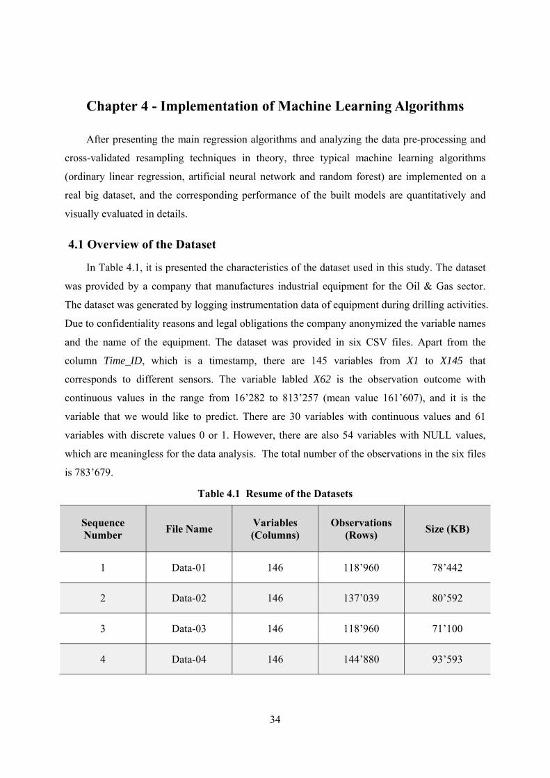
34

Chapter 4 - Implementation of Machine Learning Algorithms

After presenting the main regression algorithms and analyzing the data pre-processing and

cross-validated resampling techniques in theory, three typical machine learning algorithms

(ordinary linear regression, artificial neural network and random forest) are implemented on a

real big dataset, and the corresponding performance of the built models are quantitatively and

visually evaluated in details.

4.1 Overview of the Dataset

In Table 4.1, it is presented the characteristics of the dataset used in this study. The dataset

was provided by a company that manufactures industrial equipment for the Oil & Gas sector.

The dataset was generated by logging instrumentation data of equipment during drilling activities.

Due to confidentiality reasons and legal obligations the company anonymized the variable names

and the name of the equipment. The dataset was provided in six CSV files. Apart from the

column Time_ID, which is a timestamp, there are 145 variables from X1 to X145 that

corresponds to different sensors. The variable labled X62 is the observation outcome with

continuous values in the range from 16’282 to 813’257 (mean value 161’607), and it is the

variable that we would like to predict. There are 30 variables with continuous values and 61

variables with discrete values 0 or 1. However, there are also 54 variables with NULL values,

which are meaningless for the data analysis. The total number of the observations in the six files

is 783’679.

Table 4.1 Resume of the Datasets

Sequence Number

File Name Variables (Columns)

Observations (Rows)

Size (KB)

1 Data-01 146 118’960 78’442

2 Data-02 146 137’039 80’592

3 Data-03 146 118’960 71’100

4 Data-04 146 144’880 93’593

35

5 Data-05 146 118’960 76’122

6 Data-06 146 144’880 92’823

4.2 Data Pre-processing in R

During the data processing in this project, the R language is used extensively for

mathematical and statistical computations, and it is a flexible and powerful platform for

predictive modeling and data analysis, which can be downloaded from the Internet free of charge.

Moreover, the functions and analytical methods in the Classification and Regression Training

(caret) package are frequently used to build the model and evaluate the predictive performance

[78].

4.2.1 Filtering the Variables

After importing the six original files into R, all the constant (zero variance) variables are

found out and deleted from the dataset, which is merged from the six CSV files. In the next step,

the nearZeroVar() function in the caret package is used to filter the near zero variance variables,

which have both of the following two characteristics: The first one is that there are very few

unique values relative to the number of observations, and the second is that the frequency ratio of

the most frequent value over the second most frequent value is large. Through two steps, there

are 86 constant variables and 12 near zero variables found in the dataset. It means that there are

only 46 variables left for predictive modeling, among which 29 variables with continuous values

and 17 variables with state 0 or 1 values.

## find out the constant (zero variance) variables and delete them from the dataset 

v <‐ array(1:ncol(dataset)) 

for (i in 1:ncol(dataset)) v[i] <‐ var(dataset[,i]) 

dataset <‐ dataset[c(‐which(v==0))] 

rm(v) 

 

## find out near zero variance predictors that are have both of the  

## following characteristics: they have very few unique values  

36

## relative to the number of samples and the ratio of the frequency  

## of the most common value to the second most common value is large. 

library(caret) 

nzv <‐ nearZeroVar(dataset,saveMetrics = FALSE) 

dataset.filtered.1 <‐ dataset[ ,‐nzv] 

The third step to filter the highly correlated variables is achieved by calculating the

correlation matrix, and the correlogram of all the 46 variables can be seen in Figure 4.1. The size

of the points represents the strength of correlation between the two variables, and the blue color

and the red color are associated with the positive and negative relationship, respectively. There

are at least 11 groups of highly correlated variables, such as one group of X6, X7, X8, X9, X10,

X61, they are highly correlated with each other, but almost independent with other variables.

37

Figure 4.1 Correlogram of Variables without Near Zero Variance

The findCorrelation() function in the caret package can be used to select the variables

which are highly correlated with others for a given pair-wise absolute correlation threshold. For a

given cutoff 0.95, there are 31 variables returned, which can be deleted from the 46 variables.

Therefore, after filtering these variables, there are only 15 useful variables with 783’679

observations left in the dataset, e.g. X3, X11, X19, X42, X44, X61, X65, X68, X75, X78, X85,

X91, X113, X143, and X144.

##delete the variables which are highly correlated with others 

library(caret) 

highCorr <‐ findCorrelation(x=cor.matrix,cutoff=0.95) 

38

length(highCorr) 

dataset.filtered.2 <‐ dataset.filtered.1[ , ‐ highCorr] 

4.2.2 Transformations

As we have known in chapter 2, there are many regression models having strict

requirements to center and scale the variables, and to resolve the skewness in the variables before

modeling. The preprocess() function in the caret package can be applied to manage these

transformations (such as “BoxCox” , "center", "scale", ”pca”) to the dataset. After training the

preprocess() function, the results of the dataset transformation can be calculated by the predict

function, which looks like in Figure 4.2 by the following code:

## data transformation 

trans <‐ preProcess(dataset.filtered.2, 

                    method=c("BoxCox","center","scale")) 

transformed <‐ predict(trans,dataset.filtered.2) 

Figure 4.2 Results of the Dataset Transformations

Another place where these transformation can be set is the preProcess parameter in the train

function, a series of transformations, such as "BoxCox", "YeoJohnson", "expoTrans", "center",

"scale", "range", "knnImpute", "bagImpute", "medianImpute", "pca", "ica" and "spatialSign", can

be used during fitting the regression model.

4.2.3 PCA vs PLS

Apart from the findCorrelation() function to delete the highly correlated variables, the

Principal Components Analysis (PCA) is another effective unsupervised dimensionality

reduction procedure that can be used to transform a large number of highly correlated variables

into a small number of uncorrelated principal components, but still hold as much variability from

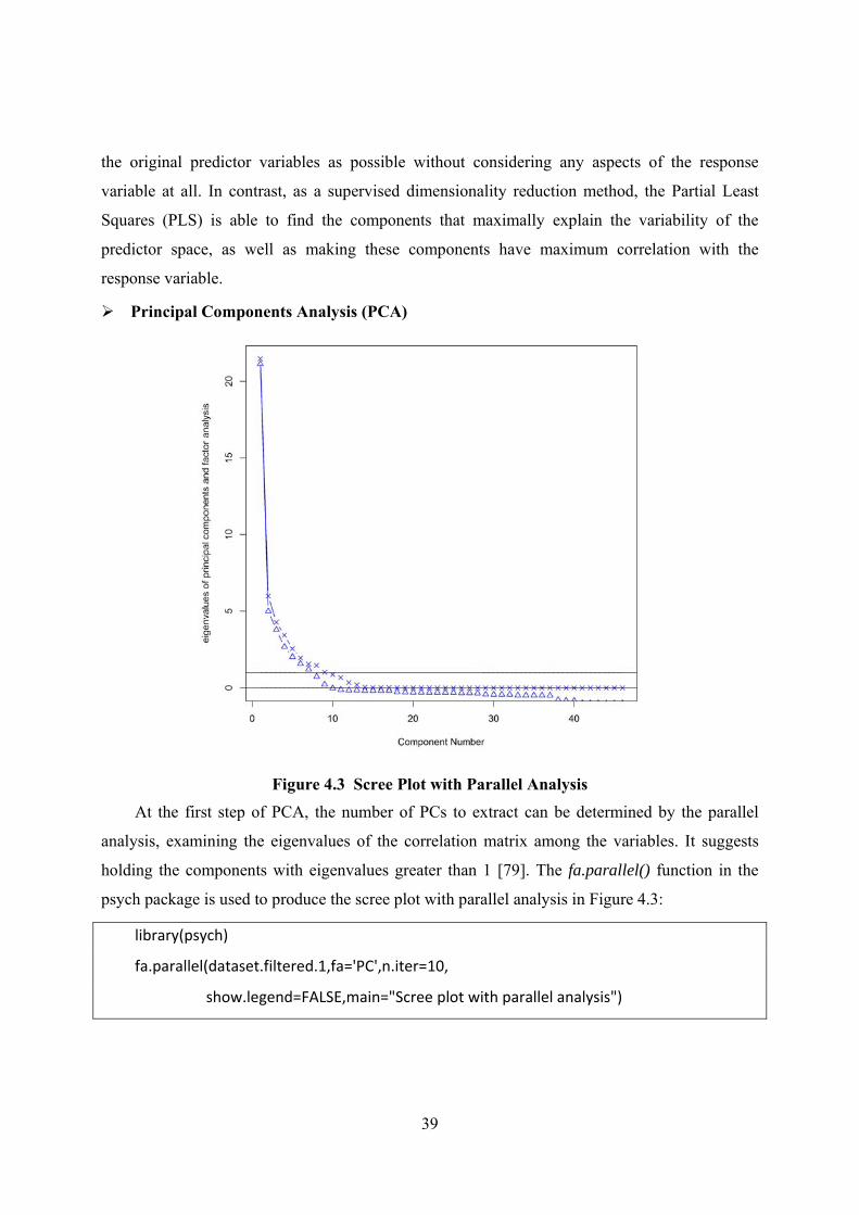
39

the original predictor variables as possible without considering any aspects of the response

variable at all. In contrast, as a supervised dimensionality reduction method, the Partial Least

Squares (PLS) is able to find the components that maximally explain the variability of the

predictor space, as well as making these components have maximum correlation with the

response variable.

Principal Components Analysis (PCA)

Figure 4.3 Scree Plot with Parallel Analysis

At the first step of PCA, the number of PCs to extract can be determined by the parallel

analysis, examining the eigenvalues of the correlation matrix among the variables. It suggests

holding the components with eigenvalues greater than 1 [79]. The fa.parallel() function in the

psych package is used to produce the scree plot with parallel analysis in Figure 4.3:

library(psych) 

fa.parallel(dataset.filtered.1,fa='PC',n.iter=10, 

               show.legend=FALSE,main="Scree plot with parallel analysis") 

40

As we can see from Figure 4.3, in the parallel analysis, the number of the eigenvalues (the

line with X’s) greater than 1 (the horizontal line) is 9, thus, it suggests the number of components

to extract is 9.

The second step is to extract the principal components based on the correlation matrix of the

dataset by the principal() function without rotation. In Figure 4.4, the column PC1 represents

the correlation between the variables and the corresponding principal components, which is also

called the component loadings. The column h2 illustrates that the amount of variance in the

variables can be explained by the 9 principal components. For instance, about 99% of the

variance in the variable X4 is explained by the 9 PCs, and 0.503% (u2) is not. The row SS

loadings is the eigenvalue of the corresponding components, which is the same as the value in

Figure 4.3, for example, the value for PC1 is 21.45. In the row Proportion Var, the PC1 explains

47% of the variance in the 46 variables, and all the 9 PCs together account for 95% of the

variance in total, which can be seen in row Cumulative Var. Finally, test of the hypothesis also

suggests that 9 components are sufficient.

Figure 4.4 Principal Components Analysis without Rotation

In the third step, rotating the principal components is used to purify the columns of the

component loading matrix, so that each column has a small number of large loadings and a

relative large number of small loadings. Applying the varimax rotation to the 46 variables, we

can get the results in Figure 4.5. Each component mainly explain a small group of variables, and

41

the percentage of variance and the eigenvalue in each individual component has changed, but the

cumulative variance for the 9 components (95%) has not changed.

Figure 4.5 Principal Components Analysis with Rotation

The goal of the PCA is to obtain scores for each observation on the 9 components, they are

saved in the scores element of the object rc, which is returned by the following function:

rc <‐ principal(dataset.filtered.1, nfactors=9, score=TRUE, rotate="varimax") 

rc$scores 

And the principal component scoring coefficients can be obtained by the following codes:

round(unclass(rc$weights),9) 

Partial Least Squares (PLS)

If the variability in the predictor variables has no apparent relationship with the response

variability, the dimensionality reduction via PCA can be misled, even not find the real predictive

relationship. As a result of this problem with PCA, the PLS is taken into account to fit the

response variable with fewer components.

The Partial Least Squares and Principal Component Regression functions in the pls package

are applied to compare the performance of these two procedures for the dataset. The PLSR owns

one tuning parameter: number of the components, which can be specified by the ncomp

argument in the plsr functions. Cross-validation is also used in the validation argument to

42

determine the optimal number of components to extract that minimize the Root Mean Squared

Error of Prediction (RMSEP). The loadings and scores functions can be used to extract the PLSR

components and scores, respectively. The main codes can be seen in the following:

library(pls) 

pcrFit <‐ pcr(Y~.,data=com.data,ncomp=14,validation="CV") 

plsFit <‐ plsr(Y~.,data=com.data,ncomp=14,validation="CV") 

summary(pcrFit) 

summary(plsFit) 

## obtaining components scores 

# scores(plsFit) 

par(mfrow=c(2,2)) 

## RMSEP: root mean squared error of prediction 

plot(pcrFit,"val",main="RMSEP in PCR") 

plot(pcrFit,"validation",val.type="R2",main="R2 in PCR") 

plot(plsFit,"val",main="RMSEP in PLSR") 

plot(plsFit,"validation",val.type="R2",main="R2 in PLSR") 

As we can see in Figure 4.6, the results show that PLSR gets the minimal RMSEP about

65’000 with 8 components, while PCR gets the same RMSEP with 13 components. Comparing

the value of R-square R2 in PCR and PLSR, we can get that only the first two components in

PLSR are able to explain about 61.15% of the relationship between the original predictor space

and the response variable, however, it requires at least 10 components to explain the same

proportion in PCR. The maximum value of R2 (73%) can be achieved by just 6 components in

PLSR, but at least 13 components in PCR. Both of the RMSEP and R2 results give us the

conclusion that the number of components retained by the unsupervised dimensionality reduction

via PCA is greater than the number of components retained by the supervised PLSR. The main

reason is that the correlation with the response variable is considered during selecting the

components of maximum variation in PLSR, but not in PCR. And another conclusion is that

even though the predictive ability (Minimum RMSEP and Maximum R2) of the two approaches

43

is almost equal, the PLSR model is much simpler because of significantly fewer components

than PCR.

Figure 4.6 Cross-validated RMSEP and R2 by Components for PLSR and PCR

4.2.4 Data Splitting

As we know, a large number of samples can be of great benefit, especially when there are

new information in the predictor space. Adding more different samples would apparently

minimize the noise in the predictors and the outcome, and improve the performance of the

44

regression model, to some extent. But it does not mean necessiarily that bigger data must give

rise to better model. As a result of the noise in the predictors and the outcome, an increase in the

number of samples would possibly lead to less positive advantages. With a sufficient number of

samples, most of models can get into stable state, adding more samples would not greatly change

the model fit. On the other hand, the cost of more samples would increase significant

computational burdens, which always require more time to build the model, more hardware to

store the data, and/or more special and feasible approaches to implement the algorithms.

For our implementation of the ordinary linear regression, artificial neural networks and

random forest algorithms, the training set and testing set can be obtained by the base R function

sample(), which is able to get random samples of the specified size from our dataset. The number

of samples in the training set and testing set is 30’000 and 15’000, respectively, accounting about

3.8% and 1.9% of the total 783’679 observations in the dataset. The outcome variable in the

training set and testing set are in the same range, as we can see the summary in Figure 4.7.

######################  Data Splitting  ####################### 

## set the random seed to reproduce the results 

set.seed(1) 

trainingRows <‐ sample(1:nrow(com.data),30000,replace=FALSE) 

trainingSet <‐ com.data[trainingRows,] 

testingRows <‐ sample(1:nrow(com.data),15000,replace=FALSE) 

testingSet <‐ com.data[testingRows,] 

Figure 4.7 Summary of the Outcome Variable in the Training Set and Testing Set

45

4.3 Ordinary Linear Regression

4.3.1 Multiple Linear Regression

First of all, the multiple ordinary linear regression is built by the lm() function with all the

30’000 samples in the training set. The model parameters and statistics is obtained by the

summary() function, which can be seen in Figure 4.8. The estimated regression coefficients in

the multiple OLR model represent that the value of the dependable variable can be increased

when the value of the independent variable is changed by one unit. For instance, the estimated

coefficient for the variable X143 is 6119.1, indicating that an increase of each unit in X143

would lead to a 6119.1 units increase in the predictive variable Y(e.g. X62), controlling for the

other variables. And the estimated coefficient is significantly different from zero with the p-value

< 2e-16. In summary, about 73.94% of the variance in the dataset can be explained by the model,

and the value of the residual standard error is 64’400.

Figure 4.8 Multiple Linear Regression Model

46

4.3.2 Measuring Performance in OLR Model

Cross-validation

Building the model is the first step on the way to do the prediction. But because the linear

regression model is only fitted for the training set, we do not know how well this model will

perform in the testing set or in the real world. Cross-validation can be used to evaluate the model

generalizability. In the k-fold cross-validation, the training set is divided into k subsets. Each of k

subsets is selected as the hold-out group, the other k-1 subsets are selected as the training group.

Since the regression model is only developed on the training group, the hand-out grouped is used

to train the model further. The performance of the hand-out groups will better reveal the model

generalizability. In our implementation, the crossval() function, which can be found in the

bootstrap package, is used to perform the 10-fold cross-validation to check the R2 statistics in

Figure 4.9.

Figure 4.9 10-fold Cross-validated R2

As we can see from Figure 4.8 and 4.9, the original R2 based on the training set without

crass-validation is 0.7394, and the new R2 with 10-fold cross-validation is 0.7389. Thus, the

change between then original R2 and the 10-fold cross-validated R2 is only 5.1e-4. The smaller

R2 change is able to tell us that the model owns better generalizability.

Quantitative Measures of Performance

47

For regression models predicting a continuous numeric outcome, the Root Mean Squared

Error (RMSE) and the coefficient of determination (R2) are often used to evaluate the

performance of the model. The former is the square root of the difference between the observed

values and the predicted outcomes, the value represents the average difference between the

observed values and the predicted outcomes. The simplest explanation of the latter is the square

of the correlation coefficients between the observed values and the predicted outcomes, its value

tells only the percentage of the information in the dataset or variation in the outcome explained

by the model, but not the accuracy.

The RMSE() and R2() functions in the caret package are used to get the two values for the

testing dataset, which can be seen in Figure 4.10. The value of the RMSE and R2 for the testing

dataset is 65556.95 and 0.7327, respectively. Although the linear regression model with a 73%

R2 is optimistic, the average distance between the observed and the predicted values is quite

large, which means that the linear regression model owns poor predictive accuracy.

Figure 4.10 Calculations of the RMSE and R2 Values

Visualizations of the Linear Regression Model Fit

Visualizations of the model fit are very useful to understand the strengths and weaknesses

of the regression model, especially the observed vs predicted plots and the predicted vs residual

plots. In Figure 4.11, the left is a plot of the observed values versus the predicted outcomes

where the R2 for the testing dataset is 0.7327, but the OLR model has a tendency to under-

predict the high observed values. The right is a plot of the predicted values versus the residual

values, in which we can find that there is no points located in the bottom left side, all the points

are apparently not randomly distributed, and the variance of the residual values is quite large.

Thus, the two plots can also give us the conclusion that the OLR model is not good enough for

the prediction.

48

Figure 4.11 Visualizations of the Linear Regression Model Fit

4.3.3 Regression Diagnostics

Before having fully confidence in the performance of the linear regression model, the

assumptions underlying our model should be evaluated and diagnosed once the regression model

is built. Regression diagnostics are a set of useful tools to evaluate and judge the performance of

the regression model. As we can see in Figure 4.12, the diagnostic plots for the multiple linear

regression model can be got by applying the plot() function to the object fit, which is returned by

the lm() function. Through analyzing the four graphs, we can get the information about the

satisfaction degree to the statistical assumptions underlying the OLR model.

Linearity

If the predicted variable is linearly related with the independent variables in the dataset,

there should be no relationship between the predicted values and the residuals. In another words,

all the variance, except for the random noise, in the dataset should be captured by the model.

However, according to the Residuals vs Fitted graph (upper left), all the points are apparently not

randomly distributed, as there is no points distributed in the bottom left side of the graph.

Normality

As we all know, in the statistical assumptions of the OLR model, the predicted variable

should be normally distributed in the case of fixed values of the independent variables. But in the

Normal Q-Q graph (upper right), a probability graph of the standardized residuals against the

49

theoretical quantiles, a majority of the points on this graph do not fall on the straight 45-degree

dash line, thus we can get the result that the normality assumption is not satisfied in this model.

Homoscedasticity

Homoscedasticity represents that the variance of the predicted variable does not change

while the levels of the independent variables are changed. If the constant variance assumption is

met, we should have a randomly distribution of the points around a horizontal line on the Scale-

Location plot (bottom left). But for this model, it is not. Thus, the homoscedasticity assumption

is also not met in this model.

Figure 4.12 Diagnostic Plots for Multiple Linear Regression Model

50

For the last graph in Figure 4.12, the Residuals vs Leverage graph (bottom right) is able to

tell us the information about the outliers, high-leverage points and influential samples in the

dataset. For example, the point 199641 seems to be a high leverage point, it may be an outlier in

the dataset. But it is worth noting that deleting the observation should be very careful, the model

should be fit to the dataset, not in the opposite direction.

As the linearity, normality and homoscedasticity assumptions are not met in this model, it

means that we cannot have fully confidence for the results of this multiple linear regression

model. Thus, two advanced and more sophisticated algorithms (artificial neural networks,

random forest) are considered in the next sections.

4.4 Artificial Neural Networks

There are a number of packages and functions for building artificial neural networks models

in R, such as nnet [80], deepnet [81], and RSNNS [82]. The nnet package is applied in this

subsection to establish the simplest single hidden-layer and feed-forward artificial neural

network. The core function nnet() in the nnet package requires several tuning parameters:

number of units in the hidden-layer, weight decay, maximum number of iterations, maximum

allowable number of weights and so on. As a result of the large number of the predictors and

observations, the whole process of the ANN model fitting would be very slow and time-

consuming by the nnet() function. Thus, before building the ANN model on the whole training

set, we are trying to find the reasonable tuning parameters by the train() function, and then some

quantitative and visual measures are taken to show the performance of the ANN model.

4.4.1 Choosing Tuning Parameters

In order to find out the reasonable values of the tuning parameters, the train() function in

caret package is implemented, in which a grid of tuning parameters for the artificial neural

networks model are set up, and a cross-validated resampling-based performance measure is also

calculated, based on a small sample (3000 observations) of the training set. A specific candidate

set of small ANN models with different number of hidden nodes from 1 to 16 and three different

values of weight decay (0.00, 0.01, and 0.10) are created. In other words, it means that there

would be 48 ANN models with different turning parameters by one run of the train() function in

Figure 4.13.

51

Figure 4.13 train() Function for Choosing ANN Tuning Parameters

As we all know, the ANN model is a non-deterministic algorithm, in which totally random

initialization may give rise to totally different results, even with the same tuning parameters.

Therefore, in this project, the above train() function has been separately run for 10 times to select

the tuning parameters with best quality. Each of the optimal result with smallest RMSE is

selected from the 48 ANN models in each run. Take the second result as an instance, in Figure

4.14, three different values (0.00, 0.01, and 0.10) of weight decay are evaluated with a single

hidden layer with sizes from 1 to 16 hidden nodes. The RMSE decreases along with the

increasing of the hidden units, and with smaller weight decay, RMSE gets smaller. The optimal

model in this run is the model with 0.00 and 13 hidden nodes.

All the ten optimal results for the ten instances of the train() function can be seen in the

following Table 4.2. All the optimal values of the weight decay are 0.00, and number of hidden

nodes ranges from 12 to 16, especially the value 13 appears 4 times. The RMSE of the ANN

model with 13 hidden nodes is the smallest value, only 0.0661 in the second and third instances.

It is worth mentioning that the values of RMSE in these models are much smaller than those of

ordinary linear regression models, since all the outcomes are divided by the maximum value of

the outcome in the 3000 observations in order to get the range within 0.0 to 1.0.

According to the optimal results of the train() function, the tuning parameters of the ANN

model by the nnet() function in the nnet package can be chosen as weight decay 0.00 and

number of hidden nodes 13 in this project.

52

Table 4.2 Optimal Results of the train() Function

Sequence Number

Weight Decay (λ)

Num. of Hidden Nodes

RMSE R2

1 0 15 0.0665 0.8685

2 0 13 0.0661 0.8692

3 0 13 0.0661 0.8696

4 0 16 0.0672 0.8670

5 0 13 0.0679 0.8629

6 0 12 0.0659 0.8717

7 0 14 0.0652 0.8733

8 0 13 0.0652 0.8737

9 0 14 0.0663 0.8696

10 0 16 0.0674 0.8665

Figure 4.14 RMSE Profiles for ANN model by train() function

53

4.4.2 Building ANN Model

In this study, a three-layered feed-forward artificial neural network is trained by the nnet()

function, and the general structure of ANN model consists one input layer (15 nodes), one

hidden layer (13 nodes) and one output layer (1 node). As we can see in Figure 4.15, the inverse

of the maximum absolute value of the large input dataset is calculated at first, which is used to

initiate the random weights on [-rang, rang]. All the outcomes are also divided by the maximum

value of the outcome in the training set in order to get the range within 0.0 to 1.0. The two

parameters size and decay are set to 13 and 0.00, which have been chosen in the last section. The

option lineout = TRUE represents that the relationship between the hidden units and the

prediction is linear, and the model is for regression. The maximum number of iterations is

changed from the default value 100 to the bigger value 5000 in order to find the parameter

estimates. The maximum allowable number of weights MaxNWts is set to

13*((ncol(trainingSet)+1)+13+1), and increasing the value would give rise to a very slow and

time consuming model training.

Figure 4.15 Artificial Neural Network Model

After building the ANN model, some related information about the model can be got by the

summary() function. The summary of the model at the first line in Figure 4.16, there are three

layers in the model, i.e. 15 nodes in the input layer, 13 nodes in the hidden layer and 1 node in

the out layer, and there are 222 weights in the model. The second line shows the options in the

model, “linear output units” tells us that the model is a regression model. In the third part, the i1,

i2… i15 are the 15 nodes in the input layer, h1, h2… h13 are the 13 nodes in hidden layer, and o1

54

is the one node in output layer. However, b is always thought as the constant item in the model.

The numeric values is the weight value from one node to other node, for example, the weight

value from the input node i4 to the hidden layer h2 is -18.93.

Figure 4.16 Summary of the ANN Model

4.4.3 Measuring Performance in ANN Model

After building the ANN model based on the training set, the main purpose of the model is to

make the corresponding prediction by the use of the model. The predict() function is applied to

make the prediction. Keep in mind that the number of the variables to make the prediction should

be the same as that of variables to train the model, or we cannot get the correct prediction result.

Quantitative Measures of Performance

As we have known before, the ANN model is a non-deterministic algorithm, which is

totally different from the deterministic ordinary linear regression algorithm. Thus, we have run

the nnet() function ten times to train ten different models based on the same training set, and

choose the best model with minimum RMSE on the testing set. The quantitative results of the

ten ANN models can be seen in Table 4.3, the best R2 we can get from the ten experiments is

0.9151 in the seventh model, and the corresponding RMSE is 36945.95, which is also the lowest

RMSE. The worst model is the ninth model, in which the RMSE and R2 are 41709.75 and 0.8920,

respectively. The RMSE and R2 even in the worst model is much better than that (RMSE =

65556.95, R2 = 0.7327) in the ordinary linear regression.

55

Table 4.3 Quantitative Results of ANN Models by the nnet() Function

Seq. Number

Weight Decay (λ)

Num. of Hidden Nodes

RMSE R2 Convergen

ce Value

1 0 13 41305.80 0.8946 0 52.8210

2 0 13 38544.30 0.9076 0 59.0791

3 0 13 40525.35 0.8980 0 61.0839

4 0 13 39572.05 0.9028 0 51.0655

5 0 13 40073.49 0.9002 0 59.8383

6 0 13 38009.82 0.9102 0 54.5844

7 0 13 36945.95 0.9151 0 48.2209

8 0 13 38291.31 0.9089 0 55.4723

9 0 13 41709.75 0.8920 0 61.5462

10 0 13 38489.25 0.9079 0 58.2260

Figure 4.17 Source Code for Quantitative Results of ANN model

All the quantitative results for each model can be got by the similar code in Figure 4.17. But

apart from the two parameters RMSE and R2, it is interesting that compare the performance of

two or more than two ANN models by the other two parameters Convergence and Value, which

are another two components of the returned value of the nnet object. If the binary value of

Convergence equals 1, it means that the maximum number of iterations is reached, otherwise 0.

Though this parameter, we can easily get the information whether the maximum number of

iterations mainly give rise to the difference of the models. From the quantitative results of ANN

model in Table 4.3, all the values of the Convergence equals 0, it at least indicates that the cause

56

of the iteration termination is due not to the maximum number of iterations during the building

process of the model. The fourth parameter Value represents the value of fitting criterion plus

weight decay term, and the less the value is, the better the model fitting is. As we can see from

the results in Table 4.3, the least value in Model 7 is 48.2209, which is apparently greater than

that in other models. It explains the fitting of the Model 7 is obviously better than that of the

other models.

Visualizations of ANN Model Fit

As illustrated in Figure 4.18, the left is the plot of observed values versus the predicted

outcomes in ANN Model 7 where the RMSE and R2 for the testing dataset are 36945.95 and

0.9151, respectively. It only has a tendency to over-predict the low observed values, and all the

other points are mainly located around the diagonal line. The right plot is of the predicted values

versus the residual values, where all the points are almost randomly distributed around the

horizontal line, apart from the bottom-left corner. Comparing with the linear regression model fit

in Figure 4.11, all the points in ANN model are closer to the diagonal line in observed vs.

predicted plot, and all the points in ANN model are not only nearer the horizontal line in

observed vs. residuals, but also the variance of those points are apparently lower than that in

Figure 4.11. Therefore, the performance of the model fit is explicitly improved by the artificial

neural network algorithm.

Figure 4.18 Visualizations of the ANN Model Fit

57

4.5 Random Forest

Random forest is an ensemble machine learning method in the case of regression, which is

mainly implemented by building a great number of decision trees during the training time and

outputting the averaging forest’s prediction of the individual trees. The randomForest package in

R can be used to build the Breiman and Cutler’s random forests model for classification and

regression [83]. The core function randomForest() in the package requires several tuning

parameters: number of trees to grow treen , number of variables at each random split selection trym

and so on.

4.5.1 Choosing Tuning Parameters

For the purpose of tuning the trym parameter, as the random forest algorithm is

computationally intensive, the train() function in the caret package is still suggested to be used

on the small number of samples in the training set, starting from 1 to 15 (total number of the

predictors). The number of trees for the random forest is also required to specify. It is worth

noting that increasing the treen will not lead to negative influence on the model, since Breiman

had proved that the random forest regression model is protected from over-fitting [45]. However,

the larger the random forest, the more time we will spend on training and building the model.

Therefore, the default value 500 trees is used in our experiment as a starting point. Then we can

train over this parameter in Figure 4.19 as follows:

Figure 4.19 train() Function for Choosing RF Tuning Parameters

As we know, the random forest regression model is also a non-deterministic algorithm, in

which randomly selected variables at each split probably give rise to totally different predictions.

Thus, the train() function is also run 10 times independently to select the table tuning parameter

with minimum RMSE and maximum R2. RMSE is also used to in the single train() function to

58

select the optimal model with the smallest value, for instance in Figure 4.20, the final value used

for the current training model is 11trym .

Figure 4.20 RMSE Profiles for RF model by train() function

All the ten optimal results for the ten instances of the train() function can be seen in the

following Table 4.4. The optimal values of the number of randomly selected variables to choose

from at each split ranges from 10 to 12, and the minimum RMSE and maximum R2 appears in

the third model with the values 29389.08 and 0.9472, respectively. According to the optimal

results of the train() function in Table 4.4, the tuning parameters of the Random Forest model by

the randomForest() function in the randomForest package can be chosen as 11trym and

500treen .

Table 4.4 Optimal Results of the train() Function

Sequence Number

ntree mtry RMSE R2

1 500 10 30234.30 0.9451

2 500 12 29566.44 0.9461

3 500 11 29389.08 0.9472

59

4 500 12 30360.70 0.9433

5 500 11 31440.05 0.9390

6 500 11 31774.48 0.9409

7 500 10 30888.30 0.9420

8 500 10 30203.17 0.9447

9 500 10 31291.42 0.9407

10 500 10 31099.17 0.9413

4.5.2 Building RF Model

After the tuning parameters choosing process, the primary implementation for the random

forest regression model can be seen in Figure 4.21. Apart from the two tuning parameters

11trym and 500treen , the option importance = TRUE represents that the variable importance

scores can be accessed, importance = FALSE means that they are not calculated as the

calculation is time consuming.

Figure 4.21 Random Forest Model

After building the Random Forest model, some profile information can be got by the print()

function. Call shows the original call to randomForest; Type illustrates the type of the training

model, it is a regression model; Number of trees means 500 trees grown in this model, and 11

predictors or variables sampled for splitting at each node; the mean of squared residuals is huge,

but about 98.08% of variance in the training set has been explained by the RF model.

60

Figure 4.22 Summary of the Random Forest Model

4.5.3 Measuring Performance in RF Model

After building the RF model based on the training set, the main purpose of the model is to

make the corresponding prediction by the model. For instance, the predict() function is applied to

make the prediction, the varImpPlot() function is used to plot the dotchart of variable importance

as measured by the random forest model, and the treesize() function is implemented to count the

size of trees in and ensemble.

Quantitative Measures of Performance

Owing to the non-deterministic characteristic of the random forest model, the

randomForest() function has been run ten times to get the best model with minimum RMSE on

the testing set. The quantitative results of the ten RF models can be seen in Table 4.5, we can

find that the values of RMSE and R2 are very stable, varying from about 30705 to 31016 and

from 0.9407 to 0.9417, respectively. The minimum RMSE and maximum R2 we can get from the

results are 30705.78 and 0.9417 in the fourth model. The worst model is the eighth model, in

which the RMSE and R2 are 31016.63 and 0.9407, respectively. Comparing with the

corresponding results in the artificial neural network model (RMSE = 36945.95, R2 = 0.9151)

and the ordinary linear regression model (RMSE = 65556.95, R2 = 0.7327), the quantitative

performance of the RF model is apparently better than both of the ANN and OLR models.

Table 4.5 Quantitative Results of RF Models by the randomForest() Function

Sequence Number

ntree mtry RMSE R2

1 500 11 30881.35 0.9412

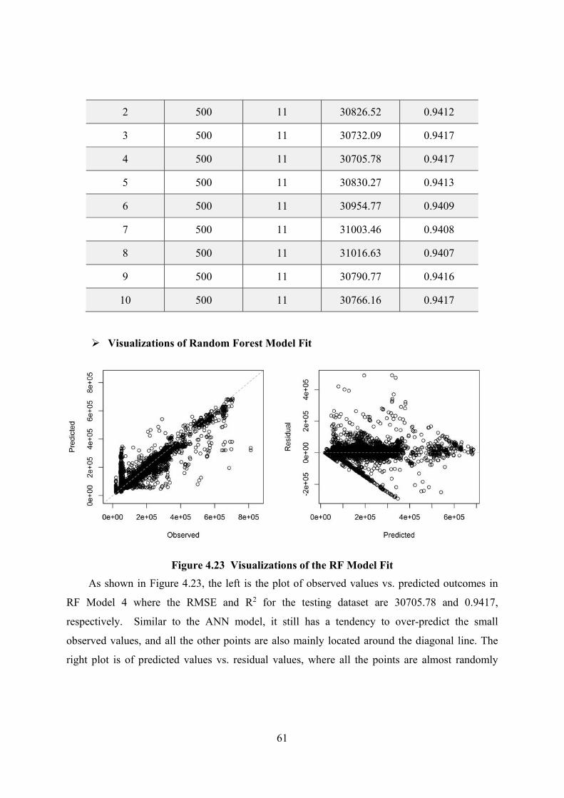
61

2 500 11 30826.52 0.9412

3 500 11 30732.09 0.9417

4 500 11 30705.78 0.9417

5 500 11 30830.27 0.9413

6 500 11 30954.77 0.9409

7 500 11 31003.46 0.9408

8 500 11 31016.63 0.9407

9 500 11 30790.77 0.9416

10 500 11 30766.16 0.9417

Visualizations of Random Forest Model Fit

Figure 4.23 Visualizations of the RF Model Fit

As shown in Figure 4.23, the left is the plot of observed values vs. predicted outcomes in

RF Model 4 where the RMSE and R2 for the testing dataset are 30705.78 and 0.9417,

respectively. Similar to the ANN model, it still has a tendency to over-predict the small

observed values, and all the other points are also mainly located around the diagonal line. The

right plot is of predicted values vs. residual values, where all the points are almost randomly

62

distributed around the horizontal line, except for the bottom-left corner due to the over-prediction

for the small values.

Visualizations of Variable Importance Scores

Figure 4.24 Variable Importance Scores for the 15 Predictors in the RF Model

As one of the specific features, as well as an important application area for the random

forest, the importance() function can be used to extract the variable importance scores. There are

two different standards to compute the influence on the model from different variables. One is

computed from permuting the out-of-bag data, and another one is computed from the total

decrease in node impurities. Thus, we are able to focus on less but more important variables

when there are a great number of variables in the dataset. The quantitative importance scores of

the fourth RF model can be seen in Figure 4.24, the first column is the names of the variables or

predictors, the second column IncMSE is the type of importance measure by mean decrease in

accuracy, and the third column IncNodePurity is by mean decrease in node impurity. The bigger

the numeric value is, the more important for the regression model the corresponding variable is.

The corresponding dot chart of variable importance scores is shown in Figure 4.25, all the

importance scores are sorted in decreasing order, and the first three variables with highest

importance scores are X3, X144 and X113, no matter in the first IncMSE measure or in the

second IncNodePurity measure. But the order of the variables with small importance scores in

different measure standards are totally different.

63

Figure 4.25 Dot-chart of Variable Importance Scores

Visualizations of Tree Size

Figure 4.26 Histogram of Tree size for the RF Model

The treesize() function can be used to count the number of nodes for the trees in the random

forest model, usually in combination with the randomForest() function and the hist() function.

As we can see in Figure 4.26, the number of nodes for each tree in the fourth random forest

64

model is different from each other. The minimum number of nodes is about 9700, but the

maximum number of nodes is above 9950.

4.6 Summary

Across the last few subsections, three typical models (Ordinary Linear Regression,

Artificial Neural Networks and Random Forest) have been implemented to the given dataset, and

the quantitative and visual performance of the built models are analyzed in details.

At first, the simplest ordinary linear regression model is built by the lm() function. Although

the OLR model can be easily interpreted, the regression diagnostics are still conducted to explain

the poorly predictive ability of the linear regression model. Only about 73.94% of the variance in

the dataset can be explained and the value of the residual standard error is 64400.

In the next step, the artificial neural network is applied by the nnet package, in which the

two parameters, number of units in the hidden-layer and weight decay, are tuned by the train()

function in caret package. The ANN model is relatively simplistic but is considered to be hard to

interpret. Because of the non-deterministic feature, the ANN model has to be implemented

several times in order to get the reasonable tuning parameters and select the optimal ANN model

with minimum RMSE and maximum R2. The performance of the model fit is explicitly improved

by the artificial neural network algorithm, where the RMSE and R2 for the testing dataset are

36945.95 and 0.9151, respectively.

At last, the random forest regression model is constructed by the randomForest() function

in the randomforest package, in which the train() function is used to tuning the parameter trym .

Comparing with the ANN model, the minimum RMSE and maximum R2 we can get from the

results are 30705.78 and 0.9417. The variable importance scores and number of nodes for each

tree is easily got by the random forest model, but the RF model training process is more complex

and more time-consuming than the other two models.

65

Chapter 5 - Conclusions

With the advent of the era of big data, machine learning has been widely used in many

technologies and industries, which is able to get computers to learn without being explicitly

programmed. As one of the fields of the supervised learning techniques, some classical models in

each type are also presented, such as Ordinary Linear Regression (OLR), Partial Least Squares

(PLS) and penalized regression in linear regression, Multivariate Adaptive Regression Splines

(MARs), Support Vector Machines (SVMs), Artificial Neural Networks (ANNs), and K-Nearest

Neighbors (KNN) in the nonlinear regression, and Bagging Tree, Random Forest and Boosted

Tree in the regression trees. The basic principal, strengths and weaknesses of each representative

model are also illustrated as well. After that, the data pre-processing and resampling techniques,

including data transformation, dimensionality reduction and k-fold cross-validation, are

explained in theory which can be used to effectively improve the performance of the training

model. During the implementation of machine learning algorithms, three typical models

(Ordinary Linear Regression, Artificial Neural Networks and Random Forest) have been

implemented by the different packages in R on the given big dataset. Apart from the model

training, the regression diagnostics are conducted to explain the poorly predictive ability of the

simplest ordinary linear regression model. Because of the non-deterministic characteristic of the

artificial neural network and random forest models, several models with small scale samples in

the dataset are built to get the reasonable tuning parameters, and the optimal models with

minimum RMSE and maximum R2 are chosen among several training models. At the last step,

the corresponding performance of the built models are quantitatively and visually evaluated in

details.

In a word, the quantitative and visual results show the feasibility for the given big dataset

under the artificial neural network and random forest models. Comparing with the ordinary linear

regression model (RMSE = 65556.95, R2 = 0.7327), the performance of the artificial neural

network (RMSE = 36945.95, R2 = 0.9151) and random forest models (RMSE = 30705.78, R2 =

0.9417) are greatly improved, but the model training process is more complex and more time-

consuming. And we also find that the right choice between different models greatly relies on the

characteristics of the dataset and the goal, and also depends upon the cross-validation technique

and the quantitative evaluation of the models.

66

References

[1]. Bishop, C.M., Pattern recognition and machine learning. Vol. 4. 2006: springer New York. [2]. Kohavi, R. and F. Provost, Glossary of terms. Machine Learning, 1998. 30(2-3): p. 271-274. [3]. Newell, A. and H.A. Simon, Human problem solving. Vol. 104. 1972: Prentice-Hall Englewood Cliffs, NJ. [4]. Michalski, R.S., A theory and methodology of inductive learning. 1983: Springer. [5]. Anderson, J.R., et al., Machine learning: An artificial intelligence approach. Vol. 2. 1986: Morgan Kaufmann. [6]. Wojtusiak, J. and K.A. Kaufman, Ryszard S. Michalski: The Vision and Evolution of Machine Learning, in Advances in Machine Learning I. 2010, Springer. p. 3-22. [7]. Inkpen, A.C., Learning and knowledge acquisition through international strategic alliances. The Academy of Management Executive, 1998. 12(4): p. 69-80. [8]. Conway, M.A., et al., Changes in memory awareness during learning: the acquisition of knowledge by psychology undergraduates. Journal of Experimental Psychology: General, 1997. 126(4): p. 393. [9]. Brown, A.L. and A.S. Palincsar, Guided, cooperative learning and individual knowledge acquisition. Knowing, learning, and instruction: Essays in honor of Robert Glaser, 1989: p. 393-451. [10]. James, G., et al., An introduction to statistical learning. 2013: Springer. [11]. Kodratoff, Y. and R.S. Michalski, Machine learning: an artificial intelligence approach. Vol. 3. 2014: Morgan Kaufmann. [12]. Baldi, P. and S. Brunak, Bioinformatics: the machine learning approach. 2001: MIT press. [13]. Webb, G.I., M.J. Pazzani and D. Billsus, Machine learning for user modeling. User modeling and user-adapted interaction, 2001. 11(1-2): p. 19-29. [14]. Carbonell, J.G., Introduction: Paradigms for machine learning. Artificial Intelligence, 1989. 40(1): p. 1-9. [15]. Ditterrich, T.G., Machine learning research: four current direction. Artificial Intelligence Magzine, 1997. 4: p. 97-136. [16]. De Garis, H. and M. Korkin, The CAM-Brain Machine (CBM): an FPGA-based hardware tool that evolves a 1000 neuron-net circuit module in seconds and updates a 75 million neuron artificial brain for real-time robot control. Neurocomputing, 2002. 42(1): p. 35-68. [17]. Bell, J., Machine Learning: Hands-On for Developers and Technical Professionals. 2014: John Wiley & Sons. [18]. Palaga, P., et al. High-performance information extraction with alibaba. in Proceedings of the 12th International Conference on Extending Database Technology: Advances in Database Technology. 2009: ACM. [19]. Saleh, B., et al., Toward automated discovery of artistic influence. Multimedia Tools and Applications, 2014: p. 1-27. [20]. Alpaydin, E., Introduction to machine learning. 2014: MIT press. [21]. Mohri, M., A. Rostamizadeh and A. Talwalkar, Foundations of machine learning. 2012: MIT press. [22]. Kuhn, M. and K. Johnson, Applied predictive modeling. 2013: Springer. [23]. Ayodele, T.O., Types of machine learning algorithms. 2010: INTECH Open Access Publisher. [24]. Bell, J., Machine Learning: Hands-On for Developers and Technical Professionals. 2014: John Wiley & Sons. [25]. Hastie, T., et al., The elements of statistical learning: data mining, inference and prediction. The Mathematical Intelligencer, 2005. 27(2): p. 83-85. [26]. Acharyya, R., A New Approach for Blind Source Separation of Convolutive Sources: Wavelet Based Separation Using Shrinkage Function. 2008: VDM, Verlag Dr. Müller. [27]. Hinton, G.E. and T.J. Sejnowski, Unsupervised learning: foundations of neural computation. 1999: MIT press. [28]. Graybill, F.A., Theory and applications of the linear model. 1976. [29]. Haenlein, M. and A.M. Kaplan, A beginner's guide to partial least squares analysis. Understanding statistics, 2004. 3(4): p. 283-297. [30]. Jolliffe, I., Principal component analysis. 2005: Wiley Online Library. [31]. Abdi, H., Partial least squares regression (PLS-regression). 2003, Thousand Oaks, CA: Sage. p. 792-795. [32]. Hoerl, A.E. and R.W. Kennard, Ridge regression: Biased estimation for nonorthogonal problems. Technometrics, 1970. 12(1): p. 55-67.

67

[33]. Tibshirani, R., Regression shrinkage and selection via the lasso. Journal of the Royal Statistical Society. Series B (Methodological), 1996: p. 267-288. [34]. Zou, H. and T. Hastie, Regularization and variable selection via the elastic net. Journal of the Royal Statistical Society: Series B (Statistical Methodology), 2005. 67(2): p. 301-320. [35]. Smola, A.J. and B. Schölkopf, A tutorial on support vector regression. Statistics and computing, 2004. 14(3): p. 199-222. [36]. Chapelle, O. and V. Vapnik. Model Selection for Support Vector Machines. in NIPS. 1999. [37]. Hakan Arslan, M., Application of ANN to evaluate effective parameters affecting failure load and displacement of RC buildings. Natural Hazards and Earth System Science, 2009. 9(3): p. 967-977. [38]. Rumelhart, D.E., G.E. Hinton and R.J. Williams, Learning internal representations by error propagation. 1985, DTIC Document. [39]. Han, E.S., G. Karypis and V. Kumar, Text categorization using weight adjusted k-nearest neighbor classification. 2001: Springer. [40]. Bentley, J.L., Multidimensional binary search trees used for associative searching. Communications of the ACM, 1975. 18(9): p. 509-517. [41]. Breiman, L., Bagging predictors. Machine learning, 1996. 24(2): p. 123-140. [42]. Büchlmann, P. and B. Yu, Analyzing bagging. Annals of Statistics, 2002: p. 927-961. [43]. Liaw, A. and M. Wiener, Classification and Regression by randomForest. R news, 2002. 2(3): p. 18-22. [44]. Svetnik, V., et al., Random forest: a classification and regression tool for compound classification and QSAR modeling. Journal of chemical information and computer sciences, 2003. 43(6): p. 1947-1958. [45]. Breiman, L., Random forests. Machine learning, 2001. 45(1): p. 5-32. [46]. Friedman, J.H., Stochastic gradient boosting. Computational Statistics & Data Analysis, 2002. 38(4): p. 367-378. [47]. Hastie, T., et al., The elements of statistical learning: data mining, inference and prediction. The Mathematical Intelligencer, 2005. 27(2): p. 83-85. [48]. Freeman, E., T.A. Frescino and G.G. Moisen, ModelMap: An R package for modeling and map production using Random Forest and Stochastic Gradient Boosting. USDA Forest Service, Rocky Mountain Research Station, 2009. 507. [49]. Breiman, L., et al., Classification and regression trees. 1984: CRC press. [50]. ÐÓÑ, Ì., An analysis of reduced error pruning. Journal of Artificial Intelligence Research, 2001. 15: p. 163-187. [51]. Bradford, J.P., et al., Pruning decision trees with misclassification costs, in Machine Learning: ECML-98. 1998, Springer. p. 131-136. [52]. Furnkranz, J. and G. Widmer. Incremental reduced error pruning. in International Conference on Machine Learning. 1994. [53]. Friedman, J.H., Greedy function approximation: a gradient boosting machine. Annals of Statistics, 2001: p. 1189-1232. [54]. Hastie, T., et al., The elements of statistical learning. Vol. 2. 2009: Springer. [55]. Ridgeway, G., Generalized Boosted Models: A guide to the gbm package. Update, 2007. 1(1). [56]. van den Berg, R.A., et al., Centering, scaling, and transformations: improving the biological information content of metabolomics data. BMC genomics, 2006. 7(1): p. 142. [57]. Bro, R. and A.K. Smilde, Centering and scaling in component analysis. Journal of Chemometrics, 2003. 17(1): p. 16-33. [58]. Geladi, P. and B.R. Kowalski, Partial least-squares regression: a tutorial. Analytica chimica acta, 1986. 185: p. 1-17. [59]. Broemeling, L.D., Box and Cox Transformation. Encyclopedia of Statistics in Quality and Reliability, 1982. [60]. Sakia, R.M., The Box-Cox transformation technique: a review. The statistician, 1992: p. 169-178. [61]. Ye, J., R. Janardan and Q. Li. Two-dimensional linear discriminant analysis. in Advances in neural information processing systems. 2004. [62]. Haeb-Umbach, R. and H. Ney. Linear discriminant analysis for improved large vocabulary continuous speech recognition. in Acoustics, Speech, and Signal Processing, 1992. ICASSP-92., 1992 IEEE International Conference on. 1992: IEEE. [63]. Roth, V. and V. Steinhage. Nonlinear discriminant analysis using kernel functions. in Advances in neural information processing systems. 1999: Citeseer. [64]. Thompson, B., Canonical correlation analysis. Encyclopedia of statistics in behavioral science, 2005. [65]. Hardoon, D., S. Szedmak and J. Shawe-Taylor, Canonical correlation analysis: An overview with

68

application to learning methods. Neural computation, 2004. 16(12): p. 2639-2664. [66]. Thompson, B., Canonical correlation analysis: Uses and interpretation. 1984: Sage. [67]. Roweis, S.T. and L.K. Saul, Nonlinear dimensionality reduction by locally linear embedding. Science, 2000. 290(5500): p. 2323-2326. [68]. de Ridder, D., et al., Supervised locally linear embedding, in Artificial Neural Networks and Neural Information Processing—ICANN/ICONIP 2003. 2003, Springer. p. 333-341. [69]. Saul, L.K. and S.T. Roweis, An introduction to locally linear embedding. unpublished. Available at: http://www. cs. toronto. edu/~ roweis/lle/publications. html, 2000. [70]. Donoho, D.L. and C. Grimes, Hessian eigenmaps: Locally linear embedding techniques for high-dimensional data. Proceedings of the National Academy of Sciences, 2003. 100(10): p. 5591-5596. [71]. Yu, L. and H. Liu. Feature selection for high-dimensional data: A fast correlation-based filter solution. in ICML. 2003. [72]. Das, S. Filters, wrappers and a boosting-based hybrid for feature selection. in ICML. 2001: Citeseer. [73]. Schölkopf, B., A. Smola and K. Müller, Kernel principal component analysis, in Artificial Neural Networks—ICANN'97. 1997, Springer. p. 583-588. [74]. Weinberger, K.Q. and L.K. Saul. An introduction to nonlinear dimensionality reduction by maximum variance unfolding. in AAAI. 2006. [75]. Jolliffe, I., Principal component analysis. 2002: Wiley Online Library. [76]. Wold, S., K. Esbensen and P. Geladi, Principal component analysis. Chemometrics and intelligent laboratory systems, 1987. 2(1): p. 37-52. [77]. Abdi, H. and L.J. Williams, Principal component analysis. Wiley Interdisciplinary Reviews: Computational Statistics, 2010. 2(4): p. 433-459. [78]. Kuhn, M., et al., caret: Classification and regression training. R package version, 2012. 2. [79]. Hayton, J.C., D.G. Allen and V. Scarpello, Factor retention decisions in exploratory factor analysis: A tutorial on parallel analysis. Organizational research methods, 2004. 7(2): p. 191-205. [80]. Ripley, B., nnet: Feed-forward neural networks and multinomial log-linear models. R package version, 2011. 7(5). [81]. Schmidhuber, J., Deep learning in neural networks: An overview. Neural Networks, 2015. 61: p. 85-117. [82]. Bergmeir, C. and J.M. Benítez, Neural networks in R using the Stuttgart neural network simulator: RSNNS. Journal of Statistical Software, 2012. 46(7): p. 1-26. [83]. Liaw, A. and M. Wiener, Classification and regression by randomForest. R news, 2002. 2(3): p. 18-22.

69

Appendix – Source Code

Data Pre-processing

## import the original files into R.  file_add <‐ "E:/UiS/MasterThesis/Dataset/Data_Students/Data‐01.csv" data_01 <‐ read.table(file_add,header=TRUE,sep=",",dec=".",row.names=NULL) file_add <‐ "E:/UiS/MasterThesis/Dataset/Data_Students/Data‐02.csv" data_02 <‐ read.table(file_add,header=TRUE,sep=",",dec=".",row.names=NULL) file_add <‐ "E:/UiS/MasterThesis/Dataset/Data_Students/Data‐03.csv" data_03 <‐ read.table(file_add,header=TRUE,sep=",",dec=".",row.names=NULL) file_add <‐ "E:/UiS/MasterThesis/Dataset/Data_Students/Data‐04.csv" data_04 <‐ read.table(file_add,header=TRUE,sep=",",dec=".",row.names=NULL) file_add <‐ "E:/UiS/MasterThesis/Dataset/Data_Students/Data‐05.csv" data_05 <‐ read.table(file_add,header=TRUE,sep=",",dec=".",row.names=NULL) file_add <‐ "E:/UiS/MasterThesis/Dataset/Data_Students/Data‐06.csv" data_06 <‐ read.table(file_add,header=TRUE,sep=",",dec=".",row.names=NULL) rm(file_add)  ## merge the observations mergedata <‐ rbind(data_01,data_02,data_03,data_04,data_05,data_06) rm(data_01,data_02,data_03,data_04,data_05,data_06)  ## delete Time_ID and the observed outcome X() dataset <‐ mergedata[c(‐1,‐63)] outcome <‐ mergedata[63] ## not mergedata[,63] colnames(outcome) <‐ c("Y")  ## check the summary of the oberveed outcome # library(Hmisc) # describe(outcome)  ## find out the constant (zero variance) variables and delete them from the dataset v <‐ array(1:ncol(dataset)) for (i in 1:ncol(dataset)) v[i] <‐ var(dataset[,i]) dataset <‐ dataset[c(‐which(v==0))] rm(v)  ## find out near zero variance predictors that are have both of the  ## following characteristics: they have very few unique values  ## relative to the number of samples and the ratio of the frequency  ## of the most common value to the frequency of the second most common value is large. 

70

library(caret) nzv <‐ nearZeroVar(dataset,saveMetrics = FALSE) dataset.filtered.1 <‐ dataset[,‐nzv]  ## calculate the correlation matrix cor.matrix <‐ cor(dataset.filtered.1)  ## plot the correlagram library(corrgram) tiff(filename="E:/UiS/MasterThesis/MasterThesisinR/corrgram.tiff",width=2400,      height=2400,res=300) corrgram(cor.matrix,order=TRUE,lower.panel=panel.shade,upper.panel=panel.pie,          text.panel=panel.txt,main="Correlogram of Variables without NZV") dev.off()  ## another way to plot the cor matrix library(corrplot) tiff(filename="E:/UiS/MasterThesis/MasterThesisinR/corrgram_1.tiff",width=2400,      height=2400,res=300) corrplot(cor.matrix,order='hclust') dev.off()  ## delete the variables which are highly correlated with others library(caret) highCorr <‐ findCorrelation(x=cor.matrix,cutoff=0.95) length(highCorr) dataset.filtered.2 <‐ dataset.filtered.1[ , ‐ highCorr]  ## data transformation trans <‐ preProcess(dataset.filtered.2,                     method=c("BoxCox","center","scale")) transformed <‐ predict(trans,dataset.filtered.2)  ############################  PCA   ###################################### ## select the number of the PCs to extract library(psych) tiff(filename="E:/UiS/MasterThesis/MasterThesisinR/screeplot.tiff",width=2400,      height=2400,res=300) fa.parallel(dataset.filtered.1,fa='PC',n.iter=10,             show.legend=FALSE,main="Scree plot with parallel analysis") dev.off()  ## extract the principal components library(psych) 

71

pc <‐ principal(dataset.filtered.1, nfactors=9, rotate="none")  ## rotating principal components rc <‐ principal(dataset.filtered.1, nfactors=9, rotate="varimax")  ## obtain principal components score ## obtaining components scores from raw data by rc$score # rc$scores  ### obtaining principal component scoring coefficients # round(unclass(rc$weights),3)  ############################################################################# ## combine the variables (without Boxcox, center, scale) and the outcome data.no.pca <‐ cbind(dataset.filtered.2,outcome)  cor.no.pca <‐ cor(data.no.pca)  library(corrgram) tiff(filename="E:/UiS/MasterThesis/MasterThesisinR/corrgram_2.tiff",width=2400,      height=2400,res=300) corrgram(cor.no.pca,order=TRUE,lower.panel=panel.shade,upper.panel=panel.pie,          text.panel=panel.txt,          main="Correlogram of Variables X and Y before transformation") dev.off()  library(corrplot) tiff(filename="E:/UiS/MasterThesis/MasterThesisinR/corrgram_3.tiff",width=2400,      height=2400,res=300) corrplot(cor.no.pca,order='hclust',          main="Correlogram of Variables X and Y before transformation") dev.off()  ############################################################################## ## combine the variables (after Boxcox, center, scale) and the outcome com.data <‐ cbind(transformed,outcome)  cor.xy <‐ cor(com.data)  library(corrgram) corrgram(cor.xy,order=TRUE,lower.panel=panel.shade,upper.panel=panel.pie,          text.panel=panel.txt, main="Correlogram of Variables X and Y after transformation")  ############################################################################## 

72

## Data Splitting set.seed(1)  library(caret) trainingRows <‐ sample(1:nrow(com.data),30000,replace=FALSE) trainingSet <‐ com.data[trainingRows,] testingRows <‐ sample(1:nrow(com.data),15000,replace=FALSE) testingSet <‐ com.data[testingRows,]  ######################### PCR VS. PLSR ############################### library(pls) pcrFit <‐ pcr(Y~.,data=com.data,ncomp=14,validation="CV") plsFit <‐ plsr(Y~.,data=com.data,ncomp=14,validation="CV")  summary(pcrFit) summary(plsFit)  ## obtaining components scores # scores(plsFit)  tiff(filename="E:/UiS/MasterThesis/MasterThesisinR/PCR_and_PLSR.tiff",      width=2400,height=2400,res=300) par(mfrow=c(2,2)) ## RMSEP: root mean squared error of prediction plot(pcrFit,"val",main="RMSEP in PCR") plot(pcrFit,"validation",val.type="R2",main="R2 in PCR") plot(plsFit,"val",main="RMSEP in PLSR") plot(plsFit,"validation",val.type="R2",main="R2 in PLSR") dev.off() 

Ordinary Linear Regression

######################Linear Regression by all the 783679 observations fit <‐ lm(Y~.,data=trainingSet) summary(fit)  ## confident interval confint(fit)  tiff(filename="E: /UiS/MasterThesis/MasterThesisinR/lmFit_with_all_dataset.tiff",      width=2400,height=2400,res=300) par(mfrow=c(2,2)) plot(fit) dev.off() 

73

 ## cross‐validation R2Check <‐ function(fit, k=10){   theta.fit <‐ function(x,y){lsfit(x,y)}   theta.predict <‐ function(fit,x){cbind(1,x)%*%fit$coef}   x <‐ fit$model[,2:ncol(fit$model)]   y <‐ fit$model[,1]   results <‐ crossval(x, y, theta.fit, theta.predict, ngroup=k)      R2 <‐ cor(y, fit$fitted.values)^2   R2cv <‐ cor(y, results$cv.fit)^2   cat("Original R‐square =", R2, "\n")   cat(k, "Fold Cross‐Validated R‐square =", R2cv, "\n")   cat("Change =", R2‐R2cv, "\n") }  R2Check(fit,k=10)  testprediction <‐ predict(fit,testingSet[,1:(ncol(testingSet)‐1)]) RMSE(testprediction,testingSet[,'Y']) R2(testprediction,testingSet[,'Y'])  tiff(filename="E: /UiS/MasterThesis/MasterThesisinR/predicted_observed_res_lmfit.tiff",      width=4800,height=2400,res=500) par(mfrow=c(1,2)) axisRange <‐ extendrange(c(testingSet[,ncol(testingSet)],testprediction)) plot(testingSet[,ncol(testingSet)],testprediction,      xlim=axisRange,      ylim=axisRange,      xlab="Observed",ylab="Predicted") abline(0,1,col="darkgrey",lty=2) plot(testprediction,testingSet[,ncol(testingSet)]‐testprediction,      xlab="Predicted",ylab="Residual") abline(h=0,col="darkgrey",lty=2) dev.off()  

Artificial Neural Networks

################### Artifical Neural Network############## mysample <‐ trainingSet[sample(1:nrow(trainingSet),3000,replace=FALSE),]  ## Create a specific candidate set of models to evaluate: nnetGrid <‐ expand.grid(.decay = c(0, 0.01, .1), 

74

                        .size = c(1:30),                                                    ## The next option is to use bagging instead of                                                       ## different random seeds.                                                      .bag = FALSE) set.seed(105)  timestart <‐ Sys.time()  ## calculate the time to run the program  nnetTune <‐ train(x = mysample[,1:(ncol(mysample)‐1)],                   y = mysample[,ncol(mysample)]/max(mysample[,ncol(mysample)]),                   method = "avNNet",                   tuneGrid = nnetGrid,                   # trControl = trainControl(method = "cv",number = 3),                   ## Automatically standardize data prior to modeling                   ## and prediction                   ##preProc = c("center", "scale"),                   ## linear relationship between hidden units and the prediction                   linout = TRUE,                   ## reduce the amount of printed output                   trace = FALSE,                   ## the number of parameters used by the model                   MaxNWts = 16 * (ncol(mysample) + 1)+ 16 + 1,                   ## the number of iterations to find parameter estimates                   maxit = 100)  nnetTune_1 <‐ train(x = mysample[,1:(ncol(mysample)‐1)],                   y = mysample[,ncol(mysample)]/max(mysample[,ncol(mysample)]),                   method = "avNNet",tuneGrid = nnetGrid,                   linout = TRUE,trace = FALSE,MaxNWts = 16 * (ncol(mysample) + 1)+ 16 + 1,                   maxit = 100) nnetTune_2 <‐ train(x = mysample[,1:(ncol(mysample)‐1)],                     y = mysample[,ncol(mysample)]/max(mysample[,ncol(mysample)]),                     method = "avNNet",tuneGrid = nnetGrid,                     linout = TRUE,trace = FALSE,MaxNWts = 16 * (ncol(mysample) + 1)+ 16 + 1,                     maxit = 100) nnetTune_3 <‐ train(x = mysample[,1:(ncol(mysample)‐1)],                     y = mysample[,ncol(mysample)]/max(mysample[,ncol(mysample)]),                     method = "avNNet",tuneGrid = nnetGrid,                     linout = TRUE,trace = FALSE,MaxNWts = 16 * (ncol(mysample) + 1)+ 16 + 1,                     maxit = 100) nnetTune_4 <‐ train(x = mysample[,1:(ncol(mysample)‐1)],                     y = mysample[,ncol(mysample)]/max(mysample[,ncol(mysample)]),                     method = "avNNet",tuneGrid = nnetGrid,                     linout = TRUE,trace = FALSE,MaxNWts = 16 * (ncol(mysample) + 1)+ 16 + 1, 

75

                    maxit = 100) nnetTune_5 <‐ train(x = mysample[,1:(ncol(mysample)‐1)],                     y = mysample[,ncol(mysample)]/max(mysample[,ncol(mysample)]),                     method = "avNNet",tuneGrid = nnetGrid,                     linout = TRUE,trace = FALSE,MaxNWts = 16 * (ncol(mysample) + 1)+ 16 + 1,                     maxit = 100) nnetTune_6 <‐ train(x = mysample[,1:(ncol(mysample)‐1)],                     y = mysample[,ncol(mysample)]/max(mysample[,ncol(mysample)]),                     method = "avNNet",tuneGrid = nnetGrid,                     linout = TRUE,trace = FALSE,MaxNWts = 16 * (ncol(mysample) + 1)+ 16 + 1,                     maxit = 100) nnetTune_7 <‐ train(x = mysample[,1:(ncol(mysample)‐1)],                     y = mysample[,ncol(mysample)]/max(mysample[,ncol(mysample)]),                     method = "avNNet",tuneGrid = nnetGrid,                     linout = TRUE,trace = FALSE,MaxNWts = 16 * (ncol(mysample) + 1)+ 16 + 1,                     maxit = 100) nnetTune_8 <‐ train(x = mysample[,1:(ncol(mysample)‐1)],                     y = mysample[,ncol(mysample)]/max(mysample[,ncol(mysample)]),                     method = "avNNet",tuneGrid = nnetGrid,                     linout = TRUE,trace = FALSE,MaxNWts = 16 * (ncol(mysample) + 1)+ 16 + 1,                     maxit = 100) nnetTune_9 <‐ train(x = mysample[,1:(ncol(mysample)‐1)],                     y = mysample[,ncol(mysample)]/max(mysample[,ncol(mysample)]),                     method = "avNNet",tuneGrid = nnetGrid,                     linout = TRUE,trace = FALSE,MaxNWts = 16 * (ncol(mysample) + 1)+ 16 + 1,                     maxit = 100) nnetTune_10 <‐ train(x = mysample[,1:(ncol(mysample)‐1)],                     y = mysample[,ncol(mysample)]/max(mysample[,ncol(mysample)]),                     method = "avNNet",tuneGrid = nnetGrid,                     linout = TRUE,trace = FALSE,MaxNWts = 16 * (ncol(mysample) + 1)+ 16 + 1,                     maxit = 100)  timeend <‐ Sys.time() runningtime <‐ timeend ‐ timestart print(runningtime)  nnetTune  tiff(filename="E:/UiS/MasterThesis/MasterThesisinR/nnetTune_2.tiff",width=2400,      height=1800,res=300) plot(nnetTune_2) dev.off()  

76

testwithall <‐ predict(nnetTune,com.data[,1:(ncol(com.data)‐1)])*max(mysample[,ncol(mysample)]) par(mfrow=c(2,1)) plot(mergedata[,'X62'])  # the dist. of the original dataset plot(testwithall)  library(caret) R2(testwithall,mergedata[,'X62']) RMSE(testwithall,mergedata[,'X62'])  ################################################# #### Artifical Neural Network with all the samples library(nnet)  timestart <‐ Sys.time()  ## calculate the time to run the program  r <‐ 1/max(abs(trainingSet[,1:(ncol(trainingSet)‐1)]))  nnetFitwithAll <‐ nnet(x = trainingSet[,1:(ncol(trainingSet)‐1)],                 y = trainingSet[,ncol(trainingSet)]/max(trainingSet[,ncol(trainingSet)]),                 # num. of nodes in hidden layer                 size = 13,                 # limit initial random weights on [‐rang,rang]                 rang = r,                 # learning rate                 decay = 0,                 # lineout TRUE represents regression, or classification                 linout = TRUE,                 ## reduce the amount of printed output                 trace = FALSE,                 ## expand the number of iterations to find parameter estimates                 maxit = 5000,                 ## and the number of parameters used by the model                 MaxNWts = 13 * (ncol(trainingSet) + 1)+ 13 + 1)  timeend <‐ Sys.time() runningtime <‐ timeend ‐ timestart print(runningtime)  nnetFitwithAll_1 <‐ nnet(x = trainingSet[,1:(ncol(trainingSet)‐1)],                        y = trainingSet[,ncol(trainingSet)]/max(trainingSet[,ncol(trainingSet)]),                        size = 13,rang = r,decay = 0,linout = TRUE,trace = FALSE,maxit = 5000,                        MaxNWts = 13 * (ncol(trainingSet) + 1)+ 13 + 1) nnetFitwithAll_2 <‐ nnet(x = trainingSet[,1:(ncol(trainingSet)‐1)], 

77

                         y = trainingSet[,ncol(trainingSet)]/max(trainingSet[,ncol(trainingSet)]),                          size = 13,rang = r,decay = 0,linout = TRUE,trace = FALSE,maxit = 5000,                          MaxNWts = 13 * (ncol(trainingSet) + 1)+ 13 + 1) nnetFitwithAll_3 <‐ nnet(x = trainingSet[,1:(ncol(trainingSet)‐1)],                          y = trainingSet[,ncol(trainingSet)]/max(trainingSet[,ncol(trainingSet)]),                          size = 13,rang = r,decay = 0,linout = TRUE,trace = FALSE,maxit = 5000,                          MaxNWts = 13 * (ncol(trainingSet) + 1)+ 13 + 1) nnetFitwithAll_4 <‐ nnet(x = trainingSet[,1:(ncol(trainingSet)‐1)],                          y = trainingSet[,ncol(trainingSet)]/max(trainingSet[,ncol(trainingSet)]),                          size = 13,rang = r,decay = 0,linout = TRUE,trace = FALSE,maxit = 5000,                          MaxNWts = 13 * (ncol(trainingSet) + 1)+ 13 + 1) nnetFitwithAll_5 <‐ nnet(x = trainingSet[,1:(ncol(trainingSet)‐1)],                          y = trainingSet[,ncol(trainingSet)]/max(trainingSet[,ncol(trainingSet)]),                          size = 13,rang = r,decay = 0,linout = TRUE,trace = FALSE,maxit = 5000,                          MaxNWts = 13 * (ncol(trainingSet) + 1)+ 13 + 1) nnetFitwithAll_6 <‐ nnet(x = trainingSet[,1:(ncol(trainingSet)‐1)],                          y = trainingSet[,ncol(trainingSet)]/max(trainingSet[,ncol(trainingSet)]),                          size = 13,rang = r,decay = 0,linout = TRUE,trace = FALSE,maxit = 5000,                          MaxNWts = 13 * (ncol(trainingSet) + 1)+ 13 + 1) nnetFitwithAll_7 <‐ nnet(x = trainingSet[,1:(ncol(trainingSet)‐1)],                          y = trainingSet[,ncol(trainingSet)]/max(trainingSet[,ncol(trainingSet)]),                          size = 13,rang = r,decay = 0,linout = TRUE,trace = FALSE,maxit = 5000,                          MaxNWts = 13 * (ncol(trainingSet) + 1)+ 13 + 1) nnetFitwithAll_8 <‐ nnet(x = trainingSet[,1:(ncol(trainingSet)‐1)],                          y = trainingSet[,ncol(trainingSet)]/max(trainingSet[,ncol(trainingSet)]),                          size = 13,rang = r,decay = 0,linout = TRUE,trace = FALSE,maxit = 5000,                          MaxNWts = 13 * (ncol(trainingSet) + 1)+ 13 + 1) nnetFitwithAll_9 <‐ nnet(x = trainingSet[,1:(ncol(trainingSet)‐1)],                          y = trainingSet[,ncol(trainingSet)]/max(trainingSet[,ncol(trainingSet)]),                          size = 13,rang = r,decay = 0,linout = TRUE,trace = FALSE,maxit = 5000,                          MaxNWts = 13 * (ncol(trainingSet) + 1)+ 13 + 1) nnetFitwithAll_10 <‐ nnet(x = trainingSet[,1:(ncol(trainingSet)‐1)],                          y = trainingSet[,ncol(trainingSet)]/max(trainingSet[,ncol(trainingSet)]),                          size = 13,rang = r,decay = 0,linout = TRUE,trace = FALSE,maxit = 5000,                          MaxNWts = 13 * (ncol(trainingSet) + 1)+ 13 + 1)  nnetFitwithAll # summary(nnetFitwithAll)  testprediction <‐ predict(nnetFitwithAll_7,                           testingSet[,1:(ncol(testingSet)‐1)])*max(trainingSet[,ncol(trainingSet)]) RMSE(testprediction,testingSet[,'Y']) R2(testprediction,testingSet[,'Y'])  

78

tiff(filename="E: /UiS/MasterThesis/MasterThesisinR/predicted_observed_res_ANNfit.tiff",      width=4800,height=2400,res=500) par(mfrow=c(1,2)) axisRange <‐ extendrange(c(testingSet[,ncol(testingSet)],testprediction)) plot(testingSet[,ncol(testingSet)],testprediction,      xlim=axisRange,      ylim=axisRange,      xlab="Observed",ylab="Predicted") abline(0,1,col="darkgrey",lty=2)  plot(testprediction,testingSet[,ncol(testingSet)]‐testprediction,      xlab="Predicted",ylab="Residual") abline(h=0,col="darkgrey",lty=2) dev.off() 

Random Forest

rfModeltr <‐ train(x = mysample[,1:(ncol(mysample)‐1)],                    y = mysample[,ncol(mysample)],                    method = "rf",                    tuneGrid = data.frame(.mtry = 1:15),                    trControl = trainControl(method = "cv"))  rfModeltr_1 <‐ train(x = mysample[,1:(ncol(mysample)‐1)],                    y = mysample[,ncol(mysample)],                    method = "rf",                    tuneGrid = data.frame(.mtry = 1:15),                    trControl = trainControl(method = "cv")) rfModeltr_2 <‐ train(x = mysample[,1:(ncol(mysample)‐1)],                      y = mysample[,ncol(mysample)],                      method = "rf",                      tuneGrid = data.frame(.mtry = 1:15),                      trControl = trainControl(method = "cv")) rfModeltr_3 <‐ train(x = mysample[,1:(ncol(mysample)‐1)],                      y = mysample[,ncol(mysample)],                      method = "rf",                      tuneGrid = data.frame(.mtry = 1:15),                      trControl = trainControl(method = "cv")) rfModeltr_4 <‐ train(x = mysample[,1:(ncol(mysample)‐1)],                      y = mysample[,ncol(mysample)],                      method = "rf",                      tuneGrid = data.frame(.mtry = 1:15),                      trControl = trainControl(method = "cv")) rfModeltr_5 <‐ train(x = mysample[,1:(ncol(mysample)‐1)], 

79

                     y = mysample[,ncol(mysample)],                      method = "rf",                      tuneGrid = data.frame(.mtry = 1:15),                      trControl = trainControl(method = "cv")) rfModeltr_6 <‐ train(x = mysample[,1:(ncol(mysample)‐1)],                      y = mysample[,ncol(mysample)],                      method = "rf",                      tuneGrid = data.frame(.mtry = 1:15),                      trControl = trainControl(method = "cv")) rfModeltr_7 <‐ train(x = mysample[,1:(ncol(mysample)‐1)],                      y = mysample[,ncol(mysample)],                      method = "rf",                      tuneGrid = data.frame(.mtry = 1:15),                      trControl = trainControl(method = "cv")) rfModeltr_8 <‐ train(x = mysample[,1:(ncol(mysample)‐1)],                      y = mysample[,ncol(mysample)],                      method = "rf",                      tuneGrid = data.frame(.mtry = 1:15),                      trControl = trainControl(method = "cv")) rfModeltr_9 <‐ train(x = mysample[,1:(ncol(mysample)‐1)],                      y = mysample[,ncol(mysample)],                      method = "rf",                      tuneGrid = data.frame(.mtry = 1:15),                      trControl = trainControl(method = "cv")) rfModeltr_10 <‐ train(x = mysample[,1:(ncol(mysample)‐1)],                      y = mysample[,ncol(mysample)],                      method = "rf",                      tuneGrid = data.frame(.mtry = 1:15),                      trControl = trainControl(method = "cv"))  timeend <‐ Sys.time() runningtime <‐ timeend ‐ timestart print(runningtime)  rfModeltr tiff(filename="E: /UiS/MasterThesis/MasterThesisinR/rfModeltr_3_plot.tiff",      width=3600,height=2400,res=500) par(mfrow=c(1,1)) plot(rfModeltr_3) dev.off()  testprediction <‐ predict(rfModeltr,testingSet[,1:(ncol(testingSet)‐1)]) RMSE(testprediction,testingSet[,'Y']) R2(testprediction,testingSet[,'Y']) 

80

 tiff(filename="E: /UiS/MasterThesis/MasterThesisinR/predicted_observed_res_rf.tiff",      width=4800,height=2400,res=500) par(mfrow=c(1,2)) axisRange <‐ extendrange(c(testingSet[,ncol(testingSet)],testprediction)) plot(testingSet[,ncol(testingSet)],testprediction,      xlim=axisRange,      ylim=axisRange,      xlab="Observed",ylab="Predicted") abline(0,1,col="darkgrey",lty=2)  plot(testprediction,testingSet[,ncol(testingSet)]‐testprediction,      xlab="Predicted",ylab="Residual") abline(h=0,col="darkgrey",lty=2) dev.off()  ###################################################### library(randomForest)  rfModel <‐ randomForest(x = trainingSet[,1:(ncol(trainingSet)‐1)],                         y = trainingSet[,ncol(trainingSet)],                         # generate importance scores or not                         importance = TRUE,                         # not be set to too small a number                         ntree = 500,                         # regression (p/3)  where p is number of variables                          mtry = 11)  timeend <‐ Sys.time() runningtime <‐ timeend ‐ timestart print(runningtime)    rfModel_1 <‐ randomForest(x = trainingSet[,1:(ncol(trainingSet)‐1)],                         y = trainingSet[,ncol(trainingSet)],                         importance = TRUE,ntree = 500,mtry = 11) rfModel_2 <‐ randomForest(x = trainingSet[,1:(ncol(trainingSet)‐1)],                          y = trainingSet[,ncol(trainingSet)],                          importance = TRUE,ntree = 500,mtry = 11) rfModel_3 <‐ randomForest(x = trainingSet[,1:(ncol(trainingSet)‐1)],                          y = trainingSet[,ncol(trainingSet)],                          importance = TRUE,ntree = 500,mtry = 11) rfModel_4 <‐ randomForest(x = trainingSet[,1:(ncol(trainingSet)‐1)],                          y = trainingSet[,ncol(trainingSet)],                          importance = TRUE,ntree = 500,mtry = 11) 

81

rfModel_5 <‐ randomForest(x = trainingSet[,1:(ncol(trainingSet)‐1)],                          y = trainingSet[,ncol(trainingSet)],                          importance = TRUE,ntree = 500,mtry = 11) rfModel_6 <‐ randomForest(x = trainingSet[,1:(ncol(trainingSet)‐1)],                          y = trainingSet[,ncol(trainingSet)],                          importance = TRUE,ntree = 500,mtry = 11) rfModel_7 <‐ randomForest(x = trainingSet[,1:(ncol(trainingSet)‐1)],                          y = trainingSet[,ncol(trainingSet)],                          importance = TRUE,ntree = 500,mtry = 11) rfModel_8 <‐ randomForest(x = trainingSet[,1:(ncol(trainingSet)‐1)],                          y = trainingSet[,ncol(trainingSet)],                          importance = TRUE,ntree = 500,mtry = 11) rfModel_9 <‐ randomForest(x = trainingSet[,1:(ncol(trainingSet)‐1)],                          y = trainingSet[,ncol(trainingSet)],                          importance = TRUE,ntree = 500,mtry = 11) rfModel_10 <‐ randomForest(x = trainingSet[,1:(ncol(trainingSet)‐1)],                          y = trainingSet[,ncol(trainingSet)],                          importance = TRUE,ntree = 500,mtry = 11)  rfModel plot(rfModel_4)  importance(rfModel_4)  tiff(filename="E:/UiS/MasterThesis/MasterThesisinR/rfModel_4_pvarImpPlot.tiff",      width=3600,height=2800,res=500) par(mfrow=c(1,1)) varImpPlot(rfModel_4) dev.off()  

tiff(filename="E:/学习/UiS/MasterThesis/MasterThesisinR/rfModel_4_treesize.tiff",      width=3600,height=2800,res=500) par(mfrow=c(1,1)) hist(treesize(rfModel_4),col='red2') box() dev.off()  testprediction <‐ predict(rfModeltr_4,testingSet[,1:(ncol(testingSet)‐1)])  RMSE(testprediction,testingSet[,'Y']) R2(testprediction,testingSet[,'Y'])  tiff(filename="E: /UiS/MasterThesis/MasterThesisinR/predicted_observed_res_rf.tiff",      width=4800,height=2400,res=500) 

82

par(mfrow=c(1,2)) axisRange <‐ extendrange(c(testingSet[,ncol(testingSet)],testprediction)) plot(testingSet[,ncol(testingSet)],testprediction,      xlim=axisRange,      ylim=axisRange,      xlab="Observed",ylab="Predicted") abline(0,1,col="darkgrey",lty=2)  plot(testprediction,testingSet[,ncol(testingSet)]‐testprediction,      xlab="Predicted",ylab="Residual") abline(h=0,col="darkgrey",lty=2) dev.off()