DEGREE PROGRAMME IN ELECTRICAL ENGINEERING

MASTER’S THESIS

VALIDATION OF CYBER-PHYSICAL SYSTEMS

IN GAS SENSOR MEASUREMENTS

Author Otto Topias Järvinen

Supervisor Géza Tóth

Second supervisor Gabriela Lorite

March 2016

Järvinen T. (2016) Validation of cyber-physical systems in gas sensor

measurements. University of Oulu, Faculty of Information Technology and

Electrical Engineering, Degree Programme in Electrical Engineering. Master’s

Thesis, p. 58.

ABSTRACT

In this thesis a cyber-physical system for gas sensor measurements was

constructed. In the design implementation, two different approaches were

taken; we created a device for calibrating and testing the sensors and another

device acting as independent battery-powered measurement platform. Both

systems are compatible with a separate circuit (sensor)board coupled within the

sensors. This board supports both commercial Taguchi-type and custom

sensors. In addition, the circuit (sensor)board includes optional heater circuits

for gas sensors as well as a separate temperature and humidity sensor.

The devices utilize Arduino-based microcontrollers and a Raspberry Pi single

board computer which were programmed to execute the specified functions.

According to the nature of cyber-physical system, devices are able to save the

data to a memory card and upload it to internet using the selected cloud service.

In order to validate the specified functionality of the devices, gas sensors were

fabricated by inkjet-printing platinum decorated tungsten(VI) oxide

nanoparticles onto a substrate. The substrate was then wire bonded to a dual in-

line package-compatible chip carrier. Test measurements and sensor calibration

were carried out in a custom test chamber in hydrogen gas environment.

Key words: Cyber-Physical Systems, embedded systems, Internet of Things, gas

sensors, tungsten trioxide, nanoparticles.

Järvinen T. (2016) Kyberfyysisten järjestelmien validointi

kaasusensorimittauksissa. Oulun yliopisto, sähkötekniikan osasto, sähkötekniikan

koulutusohjelma. Diplomityö, 58 s.

TIIVISTELMÄ

Tässä työssä valmistettiin kyberfyysinen järjestelmä kaasusensorimittauksille.

Suunniteltu toteutus sisältää kaksi lähestymistapaa; yksi laite sensoreiden

kalibrointiin ja testaukseen sekä toinen akkukäyttöinen, itsenäisenä

mittausalustana toimiva laite. Sensorit sijoitettiin erilliselle piirilevylle joka oli

yhteensopiva molempien järjestelmien kanssa. Tämä sensorikortti tukee sekä

kaupallisia Taguchi-tyyppisiä sensoreita että itsetehtyjä sensoreita. Se sisältää

myös valinnaiset lämmityspiirit kaasusensoreille sekä erillisen lämpötila- ja

kosteussensorin.

Laitteet hyödyntävät Arduino-pohjaisia mikrokontrollereita sekä Raspberry

Pi -pienoistietokonetta jotka ohjelmointiin toteuttamaan vaaditut toiminnot.

Noudattaen kyberfyysisien järjestelmien luonnetta laitteet tallentavat

mittausdatan muistikortille ja lähettävät datan valittuun pilvipalveluun.

Toiminnallisuuden todentamiseksi valmistettiin kaasusensoreita platinalla

päällystetyistä wolframitrioksidi -nanopartikkeleista. Partikkelit tulostettiin

substraatille mustesuihkutulostimella ja lankabondattiin dual in-line package-

yhteensopivaan välikappaleeseen. Mittaukset tehtiin erikoisvalmisteisessa

testikammiossa vetykaasussa.

Avainsanat: Kyberfyysiset järjestelmät, sulautetut järjestelmät, Koneiden

Internet, kaasusensorit, volframitrioksidi, nanopartikkelit.

CONTENTS

ABSTRACT

TIIVISTELMÄ

CONTENTS

ACKNOWLEDGEMENTS

ABBREVIATIONS AND SYMBOLS

1. INTRODUCTION .............................................................................................. 9

2. THEORY .......................................................................................................... 10

2.1. Cyber-Physical Systems .......................................................................... 10

2.2. Metal oxide gas sensors ........................................................................... 11

2.2.1. Sensing mechanisms .................................................................... 12

2.2.2. Pt-decorated WO3 ........................................................................ 12

2.2.3. Cross-sensitivity matrices ............................................................ 13

2.3. Hardware Specifications .......................................................................... 14

2.3.1. Microcontroller units ................................................................... 15

2.3.2. Sensor board ................................................................................ 17

2.3.3. YÚN interface board.................................................................... 20

2.3.4. Raspberry Pi interface board ....................................................... 20

2.3.5. Power supplies ............................................................................. 21

2.3.6. Displays ....................................................................................... 21

2.3.7. Test chamber ................................................................................ 22

2.4. Software specifications ............................................................................ 22

3. MANUFACTURING DEVICES ...................................................................... 23

3.1. PCBs’ design flow ................................................................................... 23

3.1.1. Sensor board ................................................................................ 23

3.1.2. YÚN interface board.................................................................... 24

3.1.3. Raspberry Pi interface board ....................................................... 25

3.2. Assembly ................................................................................................. 25

3.2.1. PCB assembly .............................................................................. 25

3.2.2. 3D printed cases ........................................................................... 26

3.3. Software design ....................................................................................... 28

3.3.1. Arduino YÚN .............................................................................. 28

3.3.2. Raspberry Pi................................................................................. 28

3.4. Gas sensors .............................................................................................. 28

3.4.1. Materials ...................................................................................... 29

3.4.2. Printing ........................................................................................ 32

3.4.3. Wire bonding ............................................................................... 33

3.5. Test chamber ........................................................................................... 34

4. RESULTS ......................................................................................................... 35

4.1. Measurements .......................................................................................... 35

4.1.1. Thermal profiling ......................................................................... 35

4.1.2. Gas measurements ....................................................................... 36

4.2. Device operation ...................................................................................... 38

5. CONCLUSIONS ............................................................................................... 40

6. REFERENCES ................................................................................................. 41

7. APPENDICES .................................................................................................. 44

ACKNOWLEDGEMENTS

This work was made in the Microelectronics Research Unit and was supported by

The University of Oulu, OPTIFU (grant number 269592) and HIPPOCAMP (grant

number 608800) projects.

I would like to thank my supervisors Docent Géza Tóth and Dr. Gabriela Lorite for

the opportunity to carry out the master’s thesis, helpful advice and reviewing. I’m

also thankful to the whole staff at Microelectronics Research Unit for support and

guidance. I would like to thank especially Anne-Riikka Rautio for assistance with

nanoparticle synthesis and constant encouragement, Rashad Hajimammadov for help

regarding wire bonding and gas lab setup, Aron Dombovari for help with inkjet

printing and Olli Pitkänen for being the selfless support.

I’m also grateful for Róbert Puskás for constructive discussion and suggestions

and Koppány Levente Juhász from the University of Szeged for transmission

electron microscope pictures. I’d also like to thank professors Krisztian Kordas and

Heli Jantunen for useful advice and confidence with the thesis.

Lastly, my greatest thanks to my beloved wife Emmi for invaluable support during

my studies.

Oulu, March 2016

Topias Järvinen

ABBREVIATIONS AND SYMBOLS

ADC Analog-to-Digital Converter

ARM Advanced RISC Machine

CAD Computer-Aided Design

CPS Cyber-Physical System

DC Direct Current

DIP Dual In-line Package

ECAD Electronic Computer-Aided Design

GPIO General Purpose Input/Output

GUI Graphical User Interface

HDMI High-Definition Media Interface

HRTEM High-Resolution Transmission Electron Microscopy

IDE Integrated Development Interface

IoT Internet of Things

ICSP In-Circuit Serial Programming

LCD Liquid Crystal Display

MCU MicroController Unit

MFC Mass Flow Controller

MOSFET Metal-Oxide-Semiconductor Field-Effect Transistor

OS Operating System

PCB Printed Circuit Board

PWM Pulse-Width Modulation

REDOX REDuction-OXidation reaction

RPi Raspberry Pi

RTOS Real Time Operating System

SMT Surface-Mount Technology

SOIC Small Outline Integrated Circuit

SPI Serial Peripheral Interface

STL STereoLithography (file format)

TFT Thin-Film-Transistor

TGS Taguchi Gas Sensor

TIG Tungsten Inert Gas welding

UI User Interface

USB Universal Serial Bus

ppm Parts per million

sccm Standard Cubic Centimeters per Minute, cm3/min

wt. % Weight percent

ABS acrylonitrile butadiene styrene

Au gold

CH4 methane

CuO copper(II) oxide

H2 hydrogen

H2O water

In2O3 indium(III) oxide

N2 nitrogen

NO nitrogen monoxide

NO2 nitrogen dioxide

NH3 ammonia

PFTE polytetrafluoroethylene

Pd palladium

Pt platinum

Pt(acac)2 platinum(II) acetylacetonate

Si silicon

SiO2 silicon dioxide

SnO2 tin(IV) oxide

TiO2 titanium

WO3 tungsten(VI) oxide / tungsten trioxide

ZnO zinc oxide

1. INTRODUCTION

The main focus of this thesis is to realize an operational cyber-physical system for

gas sensor measurements. The novel gas sensors fabricated in laboratories are

usually tested with laboratory equipment in precise conditions. The motivation for

thesis was to enable measurements indoors and outdoors without the need of

complex measurement equipment.

The work can be divided to two parts; the measurement platforms with their

respective software and the metal oxide gas sensors which are used to validate the

systems. The measurement hardware is designed and custom-built utilizing well-

established Internet of Things (IoT) platforms such as Arduino and Raspberry Pi.

Gas sensors with inkjet-printed platinum-decorated (Pt) tungsten(VI) oxide (WO3) -

nanoparticles were fabricated following the experiments in Jarmo Kukkola’s doctoral

thesis work. [1], [2]

The structure of thesis starts with a review of cyber-physical systems (CPS),

concepts involved and their designing and manufacturing processes. The operating

principles of metal oxide gas sensors are briefly discussed; Taguchi-type resistive

sensors are used as reference sensors in the platform.

Specifications are reviewed for the hardware and software design. The selection

of components and configuration is explained and the required functions of software

components are presented.

The design decisions and the printed circuit board (PCB) manufacturing flow are

described and analysed. The software structures and utilized libraries are reviewed.

Final assembly with 3D-printed cases and test calibration setup is represented.

Manufacturing process of the example metal oxide gas sensors, including

fabricating the materials, inkjet printing and wire bonding, is explained. Test setup

conditions are specified.

The experiments with used parameters and results are presented. Besides the

measurements in the test chamber the overall functionality of systems is verified.

10

2. THEORY

2.1. Cyber-Physical Systems

Recent trends in networking embedded systems into comprehensive entities have

brought up a new term Cyber-Physical System. In principle, the term is

interchangeable with embedded systems; however, CPS underlines the relationship

between the system and physical world. Aerospace, medical and defence systems,

intelligent transport infrastructure, factory and process automation as well as

environmental monitoring and control could be considered as contemporary

realizations of CPS. [3] In addition to sensors and interacting hardware, CPS also

includes the communication between parts, the processing of data and presenting it to

the end user. This holistic approach may prove to be a challenge to researchers.

Usually, research focuses on one part of the complete system, such as sensors,

electronics, networking, mathematics and control theory or user applications.

Incorporating all of these aspects to a single study is demanding, but is sometimes

required to achieve an exhaustive overview of the complete system. [4]–[8]

The hierarchy of a CPS can be organized in a simplified form, as Figure 1

presents. In embedded systems, the structure basically consists of hardware, system

software and application software layers. Although some similarities, the structure of

CPS and IoT appliances is shown in a bit different way. The lowest level is the

physical interaction level comprising of the sensors and hardware equipment. The

sensor data is then collected and managed, and sent to be analysed and archived.

Highest level is the user interaction level, which contains the application and

interpretable results.

Applications; software, user interface (UI), data display

Management of data; interpretation

Data collection and management; processing, buses

Hardware; sensors, actuators, components

Figure 1: A simplified hierarchy of a Cyber-Physical System.

The design flow of CPS begins with defining the specifications and structuring

ideas and desired functionality of the proposed system [4], [9]. The process can be

modelled in various ways: with hierarchical presentation, by data flow, using a Petri

network and so on. Hardware components and the software are specified alongside

the features to be utilized in the design process.

Hardware decisions such as keeping a measurement system unidirectional or

introducing a feedback loop to the system are influenced by the aforementioned

operation structure. Furthermore, the nature of hardware support required by the

11

equipped sensors must be considered. Desired accuracy of discretization determines

the bit depth of analog-to-digital converter (ADC). Processing power requirements

and suitable components are evaluated respecting power consumption, especially in

portable applications. Communication is even more diverse aspect and it defines both

internal buses of the device and means of transmitting the data onward from the

system.

When choosing suitable software, the most important choice is between a

conventional embedded operating system (OS) and a real-time operating system

(RTOS). Embedded operating systems usually have wider support for software

components and hardware devices. Applications with very strict timing usually

require a RTOS. Although RTOS is not as compatible with software, real-time

operating system handles interrupts and scheduling far more reliably. Application

mapping includes also defining the required functionality of the system on software

level, such as the UI and the presentation format of the data.

A simplified chart of the design flow () presented by Marwedel describes the

elements and illustrates their relations [4], [9]. The design repository is used to iterate

and keep track of the prototypes, test them and make adjustments to the

implementation. In addition, design repository acts as an information storage

connecting the resources and realized components.

Evaluation & validationAp

plic

ati

on

kn

ow

led

ge Specification

Hardware components

System software

Design repository Design

Optimization

Application mapping Testing

Figure 2: Design flow chart adapted from Marwedel. [4]

2.2. Metal oxide gas sensors

The semiconducting metal oxide gas sensors have been researched quite intensively

since their discoveries in 1950s [10]–[16]. After the initial results based on zinc

oxide (ZnO) and tin(IV) oxide (SnO2) powders, simple gas sensor structure was

patented by Taguchi [17] in 1964, which started the commercialization of these kind

of sensors. These simple and inexpensive sensors are called Taguchi gas sensors

(TGS). Nowadays the applications of metal oxide gas sensors include also

sophisticated sensors in combustion process controlling and complex sensor arrays in

chemical systems. Besides ZnO and SnO2, other metal oxides such as copper(II)

oxide (CuO), indium(III) oxide (In2O3), titanium(IV) oxide (TiO2), and tungsten(VI)

oxide (WO3) have been also extensively used. [14]–[16]

12

2.2.1. Sensing mechanisms

The basic sensing mechanism in the metal oxide semiconductor sensors is based on

reduction-oxidation (REDOX) reactions between the exposed metal oxide surface

and the target gas. These reactions affect the conductivity of the sensor surface which

can be measured. [14] In this case, the increase or decrease of conductivity depends

on the oxidizing or reducing nature of the gas and the type of the semiconductor film.

In n-type semiconductors, oxidizing gas molecules act as acceptors and decrease the

conductivity of the semiconductor; while reducing gas molecules act as donors and

increase the conductivity. In p-type semiconductor the effects are opposite. This

induced electronic change on oxide surface is called a receptor function. [14], [16],

[18], [19] On the other hand, electron transfer by the adsorption and desorption of

gas molecules also affects the width of the space charge region between the grains in

semiconductor. This causes band bending and as consequence change of conductivity

within the metal oxide. This process is called a transduction function. [16], [19]

These two functions form the basis of the gas sensing properties of metal oxides.

The sensor functionality can be affected by the type of the semiconductor and its

physical characteristics such as grain sizes and porosity. Metal additives such as

platinum (Pt), palladium (Pd) or gold (Au) have been utilized as catalysts which

reduce the activation energy in chemical reactions. In addition, the use of catalysts

enhances the sensitivity and selectivity of the sensor and improves the response and

recovery times. [20], [21]

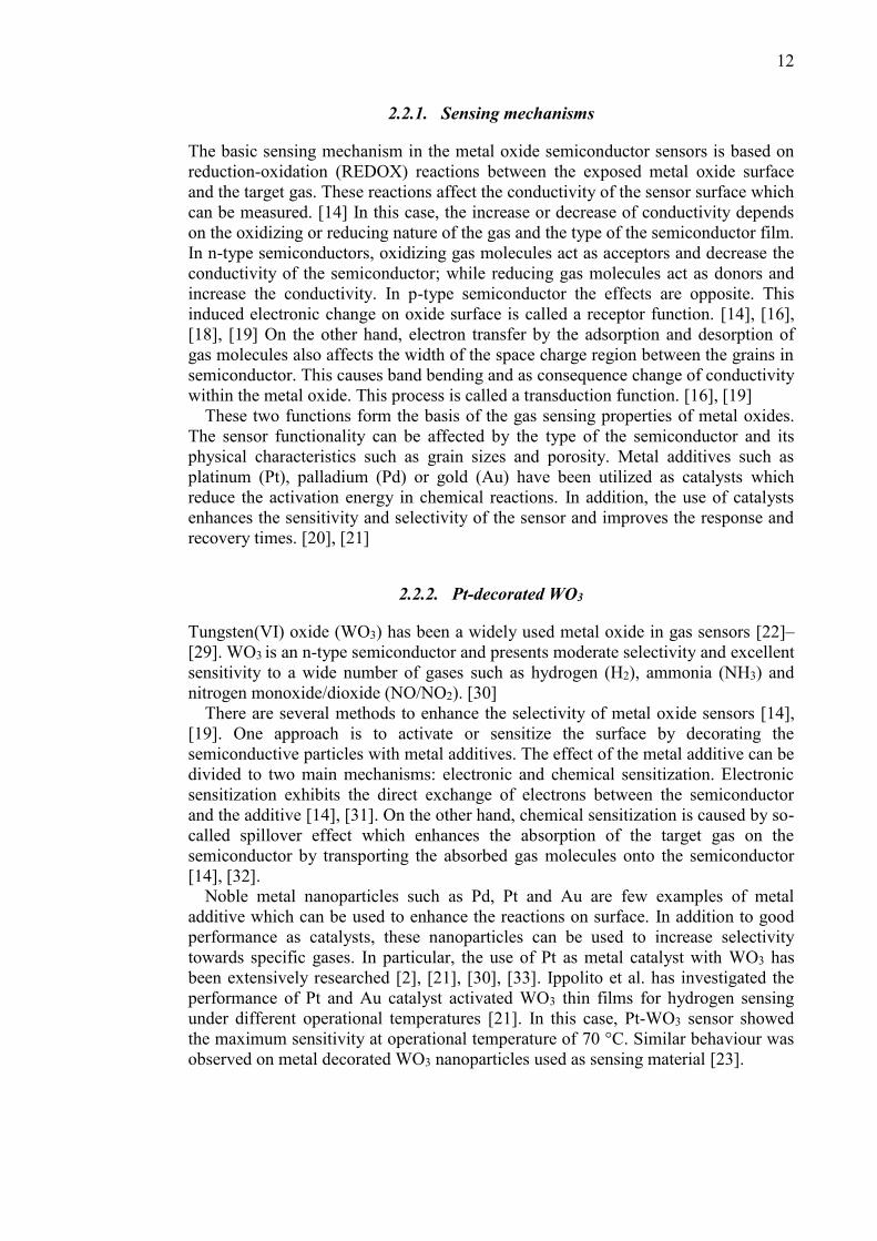
2.2.2. Pt-decorated WO3

Tungsten(VI) oxide (WO3) has been a widely used metal oxide in gas sensors [22]–

[29]. WO3 is an n-type semiconductor and presents moderate selectivity and excellent

sensitivity to a wide number of gases such as hydrogen (H2), ammonia (NH3) and

nitrogen monoxide/dioxide (NO/NO2). [30]

There are several methods to enhance the selectivity of metal oxide sensors [14],

[19]. One approach is to activate or sensitize the surface by decorating the

semiconductive particles with metal additives. The effect of the metal additive can be

divided to two main mechanisms: electronic and chemical sensitization. Electronic

sensitization exhibits the direct exchange of electrons between the semiconductor

and the additive [14], [31]. On the other hand, chemical sensitization is caused by so-

called spillover effect which enhances the absorption of the target gas on the

semiconductor by transporting the absorbed gas molecules onto the semiconductor

[14], [32].

Noble metal nanoparticles such as Pd, Pt and Au are few examples of metal

additive which can be used to enhance the reactions on surface. In addition to good

performance as catalysts, these nanoparticles can be used to increase selectivity

towards specific gases. In particular, the use of Pt as metal catalyst with WO3 has

been extensively researched [2], [21], [30], [33]. Ippolito et al. has investigated the

performance of Pt and Au catalyst activated WO3 thin films for hydrogen sensing

under different operational temperatures [21]. In this case, Pt-WO3 sensor showed

the maximum sensitivity at operational temperature of 70 °C. Similar behaviour was

observed on metal decorated WO3 nanoparticles used as sensing material [23].

13

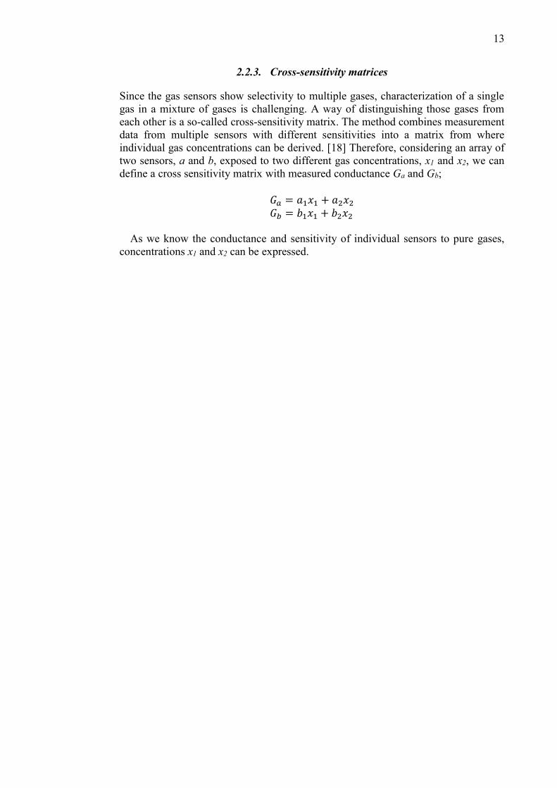
2.2.3. Cross-sensitivity matrices

Since the gas sensors show selectivity to multiple gases, characterization of a single

gas in a mixture of gases is challenging. A way of distinguishing those gases from

each other is a so-called cross-sensitivity matrix. The method combines measurement

data from multiple sensors with different sensitivities into a matrix from where

individual gas concentrations can be derived. [18] Therefore, considering an array of

two sensors, a and b, exposed to two different gas concentrations, x1 and x2, we can

define a cross sensitivity matrix with measured conductance Ga and Gb;

𝐺𝑎 = 𝑎1𝑥1 + 𝑎2𝑥2 𝐺𝑏 = 𝑏1𝑥1 + 𝑏2𝑥2

As we know the conductance and sensitivity of individual sensors to pure gases,

concentrations x1 and x2 can be expressed.

14

2.3. Hardware Specifications

The measurement device design was divided into two different systems. The two

systems and relationships between components are described in Figure 3. One

system utilises the Arduino YÚN board and is to be used in laboratory environment

plugged into the mains. An emergency backup battery was considered to be a future

add-on. The other system uses a Raspberry Pi 2 and it is designed to act as an

independent and portable unit so it contains also a built-in battery.

Much similar to so-called shield interfaces, interposer printed circuit boards were

manufactured to be able to connect the sensor board to microcontrollers via standard

pin header spacing and arrangements. These interface boards include power

regulators from 12-18 V direct current (DC) source as well. The sensor board is not

integrated in any of the systems and it was designed to be compatible to both of

them. The sensor board consists of gas sensors, heater components, temperature and

humidity sensors as well as an ADC. In addition, the sensor board has two kinds of

connector interfaces: a 2x8 pin header for YÚN system and a serial DB-15 connector

for the Raspberry Pi (RPi) system. Furthermore, both systems include a display for

observing the measured values. Other required functionality was the ability to store

and send the measurement data. Finally, tailored enclosures are 3D printed and

devices are assembled to be fully working. Besides the basic operation, the system

performance was evaluated for gas sensing using a custom-made test chamber.

Sensor board

YÚN interface

board

Rpi interface board

DC power

Arduino YÚN Raspberry Pi 2

Battery DC power

Display

microSD card

Display

YÚN system Raspberry Pi system

InternetInternet

microSD card

Figure 3: The hierarchy of systems.

15

2.3.1. Microcontroller units

The microcontrollers were chosen considering the available community support and

the high level of integration (e.g. on-board Wi-Fi chip). To unify the syntax of the

software code and interfaces with sensor boards, an Atmel ATMEGA328P-PU

microcontroller was added to the Raspberry Pi interface board, acting between RPi

and the ADC on the sensor board.

2.3.1.1. Arduino YÚN

Arduino YÚN (Arduino LLC) is one of the most versatile platforms in Arduino line

of products (Picture 1). Besides the basic functionality shared by all Arduino boards,

it accompanies a Wi-Fi chip and a microSD card reader. YÚN is based on

ATmega32u4 microcontroller. [34] In this work, we programmed in the Arduino

integrated development interface (IDE) (version 1.6.4) with embedded C. YÚN

device is shown in Picture 1.

Picture 1: Arduino YÚN.

16

2.3.1.2. Raspberry Pi 2

Raspberry Pi 2 Model B (Raspberry Pi Foundation) was chosen because its wide

support of peripherals and software (Picture 2). RPi 2 Model B has a Quad-core

Advanced RISC Machine (ARM) processor running at 800 MHz, 1GB of DDR2

RAM and 27 general purpose input/output (GPIO) pins. OS, which can be a variety

of different embedded Linux distributions, is run from a microSD card. In addition,

RPi 2 presents 4 Universal Serial Bus (USB) ports, a High-Definition Media

Interface (HDMI) port and a RJ-45 connector available for peripherals. [35]

Raspberry Pi 2 is a competent system for its form factor and presents quite

extensive software capabilities since it runs an ARM distribution of Linux. The

system is running on Raspbian free operating system, which is a custom-made

distribution for the RPi based on Debian 8. The version used in this work was

released on 2015-09-24 and had Kernel version 4.1. The graphical user interface

(GUI) and connectivity with the microcontroller unit (MCU) on interface board is

written with Python (version 2.7) and the interposing MCU is programmed with

embedded C in Arduino IDE.

Picture 2: Raspberry Pi 2.

17

2.3.2. Sensor board

The sensor board includes four sensor sockets, trimmer potentiometers for adjusting

the sensitivity of sensors, four metal-oxide-semiconductor field-effect transistors

(MOSFET) with flywheel diodes for regulating the heater voltage, MCP3008 ADC

[36] and a DB-15 serial connector providing connectivity with RPi system and

calibration setup. (Picture 3) ADC and digital logic use 3.3 V as their operating

voltage which is compatible with both YÚN and RPi. Heater voltage is regulated by

pulse-width modulation (PWM) between 0-5 V.

Picture 3: The sensor board.

2.3.2.1. Sensors

In order to verify the compatibility of the wide-used Taguchi-type commercial

sensors with the developed systems, two different kinds of Taguchi sensors were

chosen with strong selectivity to certain gases (Picture 4). MQ-4 acted as a

selectivity reference sensor and MQ-8 was particularly suitable for comparisons with

the WO3 sensors. The former is especially sensitive to methane (CH4) and latter to

hydrogen (H2) [37], [38]. These sensors are attached to the sensor board via

corresponding sockets, which enables switching sensors without the need of re-

soldering.

Picture 4: Various Taguchi sensors and a sensor socket on the right.

18

Aside from these commercial sensors, custom sensors based on Pt-decorated WO3

nanoparticles were designed and fabricated. These inkjet-printed sensors were wire

bonded to a chip carrier. A 24-pin dual-inline package (DIP) chip carrier from

Kyocera was chosen once presents adequate footprint to fit the sensor chips and the

DIP standard is widely used (Picture 5). Sockets were again used to ensure solderless

swapping of sensors.

Picture 5: A Kyocera chip carrier and respective DIP socket.

2.3.2.2. Temperature and humidity sensor

As the resistance curves of gas sensor varies according to the temperature and

humidity of test environment, a separate temperature / humidity sensor was added to

sensor board to calibrate measures according to the conditions (Picture 6). For this

purpose, a fairly accurate sensor, DHT22 was chosen [39] and connected to 3.3 V

operating voltage.

Picture 6: DHT22 temperature and humidity sensor.

19

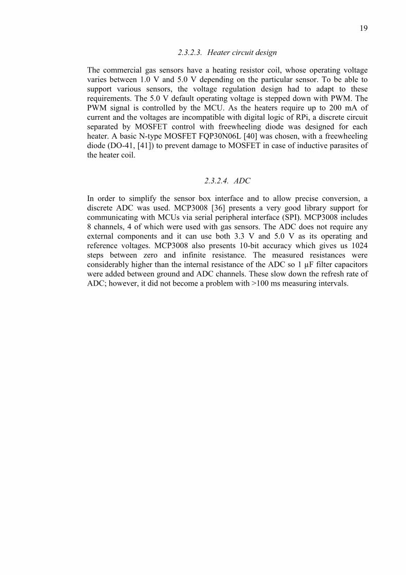
2.3.2.3. Heater circuit design

The commercial gas sensors have a heating resistor coil, whose operating voltage

varies between 1.0 V and 5.0 V depending on the particular sensor. To be able to

support various sensors, the voltage regulation design had to adapt to these

requirements. The 5.0 V default operating voltage is stepped down with PWM. The

PWM signal is controlled by the MCU. As the heaters require up to 200 mA of

current and the voltages are incompatible with digital logic of RPi, a discrete circuit

separated by MOSFET control with freewheeling diode was designed for each

heater. A basic N-type MOSFET FQP30N06L [40] was chosen, with a freewheeling

diode (DO-41, [41]) to prevent damage to MOSFET in case of inductive parasites of

the heater coil.

2.3.2.4. ADC

In order to simplify the sensor box interface and to allow precise conversion, a

discrete ADC was used. MCP3008 [36] presents a very good library support for

communicating with MCUs via serial peripheral interface (SPI). MCP3008 includes

8 channels, 4 of which were used with gas sensors. The ADC does not require any

external components and it can use both 3.3 V and 5.0 V as its operating and

reference voltages. MCP3008 also presents 10-bit accuracy which gives us 1024

steps between zero and infinite resistance. The measured resistances were

considerably higher than the internal resistance of the ADC so 1 µF filter capacitors

were added between ground and ADC channels. These slow down the refresh rate of

ADC; however, it did not become a problem with >100 ms measuring intervals.

20

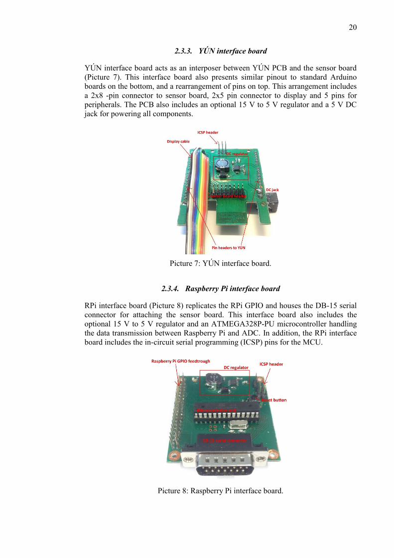
2.3.3. YÚN interface board

YÚN interface board acts as an interposer between YÚN PCB and the sensor board

(Picture 7). This interface board also presents similar pinout to standard Arduino

boards on the bottom, and a rearrangement of pins on top. This arrangement includes

a 2x8 -pin connector to sensor board, 2x5 pin connector to display and 5 pins for

peripherals. The PCB also includes an optional 15 V to 5 V regulator and a 5 V DC

jack for powering all components.

Picture 7: YÚN interface board.

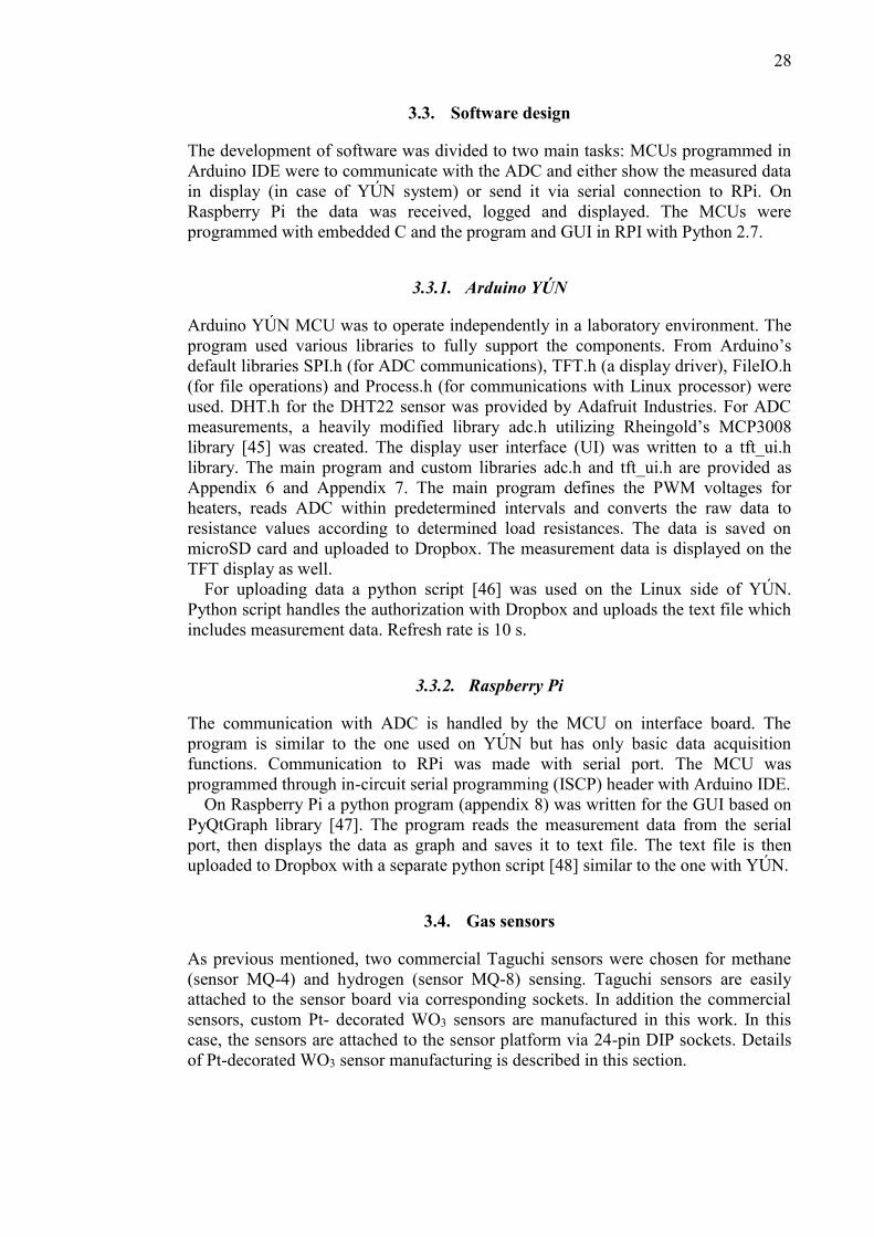
2.3.4. Raspberry Pi interface board

RPi interface board (Picture 8) replicates the RPi GPIO and houses the DB-15 serial

connector for attaching the sensor board. This interface board also includes the

optional 15 V to 5 V regulator and an ATMEGA328P-PU microcontroller handling

the data transmission between Raspberry Pi and ADC. In addition, the RPi interface

board includes the in-circuit serial programming (ICSP) pins for the MCU.

Picture 8: Raspberry Pi interface board.

21

2.3.5. Power supplies

For the portable system, a battery was needed to ensure on-the-go operation.

Simultaneous charging of the battery while operating was also a requirement for the

continuous measurements. In order to simplify the design, an existing power bank

was used (Xiaomi Mi, 10000 mAh) which supplies 2.1 A at 5.1 V.

For the Arduino YÚN based system, a power regulator circuit which could convert

12 V to 15 V input voltage to the 5 V was designed. An ADP2303 ([42], Analog

Devices, Inc.) regulator supplying 3 A was chosen to the regulator circuit. At first a

separate regulator PCB was made to verify the desired performance. Then the design

was implemented on the interface boards.

2.3.6. Displays

Arduino YÚN based system uses a standard Arduino LCD display shield, which

presents a 1.77” 160x128 pixel display area [43]. The display is connected to the

interface board. On the other hand, the Raspberry Pi based system uses a standard

display unit from Adafruit, which has a 2.8” resistive touch screen with 320x240

resolution TFT display [44]. In this case, the display is connected to the standard

GPIO pins on interface board which are replicated from the RPi below. The display

units are shown in Picture 9.

Picture 9: Display units. Arduino YÚN’s display on the left and Raspberry Pi's

display on the right.

22

2.3.7. Test chamber

A test chamber was manufactured in order to evaluate the sensors performance.

(Picture 10) The chamber includes 3 KF40 -type flanges and volume of 1500 cm3.

This chamber was used to calibrate the system and test the inkjet-printed sensors.

The computer-aided design (CAD) drawing of the chamber is presented in Appendix

4. To enhance the distribution of gas flow, a fan (50mm, 12 V default voltage, driven

at 5 V, Titan Computer Co. Ltd.) was added to the chamber. A 50 x 50 mm, 40W

Kapton® foil heater (317-KAPH-2/2-V2, Allectra) was used to heat the chamber up

to 75 °C (maximum temperature provided by the heater).

Picture 10: Test chamber.

2.4. Software specifications

The basic functionality of the software is to read the ADC channels, store and upload

the data and graphically show the sensor response. These functions are implemented

on several software levels. Microcontrollers monitor resistance values from the ADC

via SPI bus as well as the temperature and humidity data from the DHT22 sensor. In

addition, they control the voltage of the heater circuits with PWM.

Arduino YÚN -platform carries out the basic processing of data and uploads it to

cloud service (Dropbox, Dropbox Inc.). Values are also shown on a TFT screen. This

platform is also used to calibrate the sensors. In calibration, only the sensor board is

in the test chamber. A serial cable connects the sensor board to the YÚN, outside the

chamber. During calibration, measurement data is saved to a microSD card. All

programming is done with the Arduino IDE, version 1.6.4.

On RPi -platform, MCU handles only the data acquisition. Raw data is then sent to

RPi via serial port to be processed onward. Raspberry Pi stores the data to a txt file,

uploads the file to cloud and shows the raw ADC data on a LCD screen in real time.

This graphical user interface is written with Python.

23

3. MANUFACTURING DEVICES

3.1. PCBs’ design flow

As the specifications and requirements changed during the initial development

process, the layout designs were iterated a couple of times. Main tasks with iterations

were introducing new functions, optimizing board layout and wiring and correcting

occasional layout mistakes. The fundamental features of the platform are naturally

preserved and designed to allow easy alterations to the implementation.

The schematics and layout designs were made with open-source electronic

computer-aided design (ECAD) software, KiCad (version 3.0.2). KiCad presents

comprehensive features for schematic drawing, footprints creation, management and

layout design. Although lacking some advanced options of commercial product

suites, KiCad has powerful basic tools far exceeding the requirements of this

master’s thesis. Reference design for ADP2303 [42] was utilized with the regulator

design.

3.1.1. Sensor board

The sensor board PCBs first draft was 93 x 92 mm, which was later optimized to 63

x 70 mm. The final sensor board layout is shown in Figure 4. The schematic for the

sensor board is presented as Appendix 1. The sensor board arranges the 4 sensors and

the temperature/humidity sensor in a ring with ADC and connectors on bottom part

of the layout. Adjustable load resistances and test points are located in the centre. In

order to reduce the footprint of the board some components, such as heater

assemblies were located on underside. The board connects to YÚN interface board

with a standard 2x8 pin header. In addition, this board includes four mounting holes

with identical layout to Arduino boards.

24

Figure 4: Layout of the finalized sensor board.

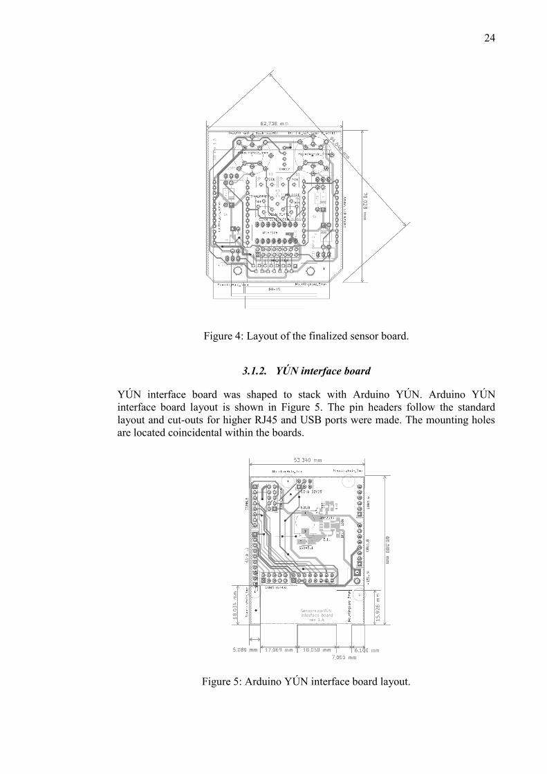
3.1.2. YÚN interface board

YÚN interface board was shaped to stack with Arduino YÚN. Arduino YÚN

interface board layout is shown in Figure 5. The pin headers follow the standard

layout and cut-outs for higher RJ45 and USB ports were made. The mounting holes

are located coincidental within the boards.

Figure 5: Arduino YÚN interface board layout.

25

3.1.3. Raspberry Pi interface board

Instead of a cut-out RPi interface board was made to be shorter than the RPi. The RPi

interface board layout is presented in Figure 6. This interface board extends the

GPIO header from RPi to the display panel on the top of the stack. In addition, the

board includes a male DB-15 serial connector for connecting the sensor board to the

system.

Figure 6: Raspberry Pi 2 interface board layout.

3.2. Assembly

Besides soldering the components to circuit boards, complete assembly process

included also stacking the boards, enclosing them to 3D printed cases and testing the

operation.

3.2.1. PCB assembly

Most surface-mount technology (SMT) components were soldered by hand (Weller®

WS 81 soldering station with WSP 80 soldering iron, Henkel Multicore® solder,

60/40 % Sn/Pb alloy, 0,32 and 0,7 mm diameters), only the small outline integrated

circuit (SOIC) packaging of the ADP2303 regulator required reflow soldering. In this

particular case, a reflow oven (LPKF ProtoFlow, LPKF Laser Electronics AG) was

used. Spacer nuts (M3/6 mm, brass) were used to support stacking the boards

alongside the supports in cases.

26

3.2.2. 3D printed cases

The 3D printed cases were designed with Autodesk Inventor Professional 2016

(Autodesk Inc.) and exported to a .stl (STereoLithography) format. The enclosures

were then printed with Makerbot Replicator X2 (MakerBot Industries) using fused

filament fabrication technology (Picture 11 and Picture 12), where acrylonitrile

butadiene styrene (ABS) filament was used as printing material.

Picture 11: Printing in process.

Picture 12: MakerBot Replicator 2X.

27

The 3D printed cases have openings for all ports and have clasps for securing the

lids. The empty cases with their lids can be seen in Picture 13. Complete assembly

and exploded view for Raspberry Pi system is shown in Figure 7.

Picture 13: 3D printed cases.

Figure 7: Complete assembly of the Raspberry Pi system.

28

3.3. Software design

The development of software was divided to two main tasks: MCUs programmed in

Arduino IDE were to communicate with the ADC and either show the measured data

in display (in case of YÚN system) or send it via serial connection to RPi. On

Raspberry Pi the data was received, logged and displayed. The MCUs were

programmed with embedded C and the program and GUI in RPI with Python 2.7.

3.3.1. Arduino YÚN

Arduino YÚN MCU was to operate independently in a laboratory environment. The

program used various libraries to fully support the components. From Arduino’s

default libraries SPI.h (for ADC communications), TFT.h (a display driver), FileIO.h

(for file operations) and Process.h (for communications with Linux processor) were

used. DHT.h for the DHT22 sensor was provided by Adafruit Industries. For ADC

measurements, a heavily modified library adc.h utilizing Rheingold’s MCP3008

library [45] was created. The display user interface (UI) was written to a tft_ui.h

library. The main program and custom libraries adc.h and tft_ui.h are provided as

Appendix 6 and Appendix 7. The main program defines the PWM voltages for

heaters, reads ADC within predetermined intervals and converts the raw data to

resistance values according to determined load resistances. The data is saved on

microSD card and uploaded to Dropbox. The measurement data is displayed on the

TFT display as well.

For uploading data a python script [46] was used on the Linux side of YÚN.

Python script handles the authorization with Dropbox and uploads the text file which

includes measurement data. Refresh rate is 10 s.

3.3.2. Raspberry Pi

The communication with ADC is handled by the MCU on interface board. The

program is similar to the one used on YÚN but has only basic data acquisition

functions. Communication to RPi was made with serial port. The MCU was

programmed through in-circuit serial programming (ISCP) header with Arduino IDE.

On Raspberry Pi a python program (appendix 8) was written for the GUI based on

PyQtGraph library [47]. The program reads the measurement data from the serial

port, then displays the data as graph and saves it to text file. The text file is then

uploaded to Dropbox with a separate python script [48] similar to the one with YÚN.

3.4. Gas sensors

As previous mentioned, two commercial Taguchi sensors were chosen for methane

(sensor MQ-4) and hydrogen (sensor MQ-8) sensing. Taguchi sensors are easily

attached to the sensor board via corresponding sockets. In addition the commercial

sensors, custom Pt- decorated WO3 sensors are manufactured in this work. In this

case, the sensors are attached to the sensor platform via 24-pin DIP sockets. Details

of Pt-decorated WO3 sensor manufacturing is described in this section.

29

3.4.1. Materials

The Pt-decorated WO3 nanoparticles were prepared as previously described in [2].

In order to prepare 1 wt.% Pt / WO3 mixture (named ARHR-AC15), 18 mg of

platinum(II) acetylacetonate (Pt(acac)2) were dissolved in 175 ml of acetone and

mixed with 0.875 g WO3 nanoparticles (550086, Aldrich) by sonicating for 2 hours,

followed by stirring at room temperature for 4 hours. Remaining acetone was

evaporated using stirring plate at 150 °C, and leaving the mixture overnight in oven

at 80 °C. The powder was then calcinated for 2 hours at 300 °C, with heating rate of

5 °C/min and reduced for 3 hours in 200 °C, with similar heating rate. Similarly, a

second batch was prepared but not reduced (named OTJ-AA3). The nanoparticles

were analysed with high-resolution transmission electron microscopy (HRTEM, FEI

Tecnai G2 20 X-TWIN, 200 kV accelerating voltage) in collaboration with

University of Szeged (Figure 8 and Figure 9).

Figure 8: HRTEM micrograph of Pt-decorated WO3 nanoparticles (sample ARHR-

AC15). Inset: Pt nanoparticles can be seen as smaller and darker areas.

30

Figure 9: HRTEM micrograph of Pt-decorated WO3 nanoparticles (sample OTJ-

AA3). Inset: Pt nanoparticles can be seen as smaller and darker areas.

In order to inkjet print the Pt-decorated WO3 nanoparticles, inks were initially

prepared with a 50/50 wt. % 2,3-butanediol/deionized water which proved to be

easily printable. However, this preparation produced poor results with

distinguishable coffee ring effects, probably caused by the slow solvent evaporation.

In addition, this first attempted showed a very low conductance. A subsequent batch

of inks were prepared with 100 % distilled H2O. The water-based inks produced

significantly better results, although jetting from cartridges provided to be more

difficult. In future works, optimization on suspension rheology will be necessary.

Based on these results, two types of inks were prepared: OTJ-AA4 using reduced Pt-

decorated WO3 nanoparticles (ARHR-AC15, Figure 8) and OTJ-AA5 using a non-

reduced Pt-decorated WO3 nanoparticles (OTJ-AA3, Figure 9). For both cases, 20

mg of nanoparticles powder was mixed with 20 g of distilled H2O via sonication for

3 hours.

The solutions were left to sediment overnight in room temperature. The

sedimentation of suspensions consisted of three parts: clear topmost layer (about 5

31

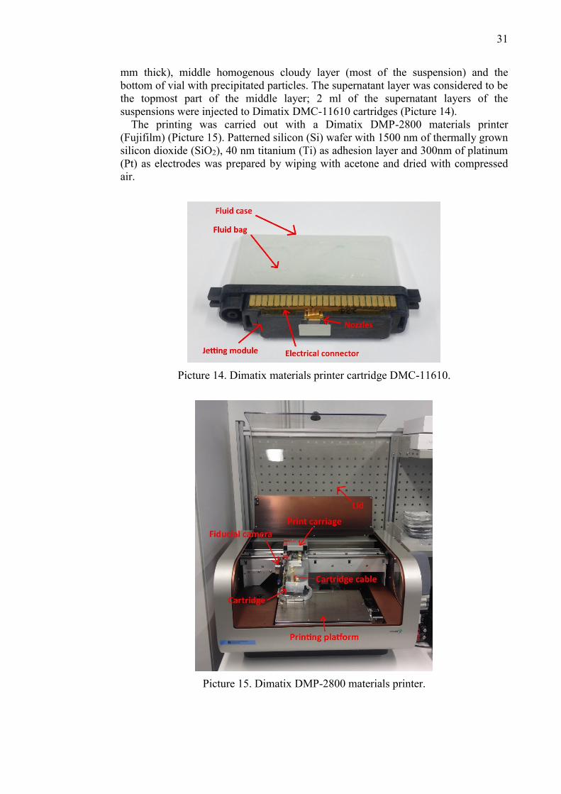
mm thick), middle homogenous cloudy layer (most of the suspension) and the

bottom of vial with precipitated particles. The supernatant layer was considered to be

the topmost part of the middle layer; 2 ml of the supernatant layers of the

suspensions were injected to Dimatix DMC-11610 cartridges (Picture 14).

The printing was carried out with a Dimatix DMP-2800 materials printer

(Fujifilm) (Picture 15). Patterned silicon (Si) wafer with 1500 nm of thermally grown

silicon dioxide (SiO2), 40 nm titanium (Ti) as adhesion layer and 300nm of platinum

(Pt) as electrodes was prepared by wiping with acetone and dried with compressed

air.

Picture 14. Dimatix materials printer cartridge DMC-11610.

Picture 15. Dimatix DMP-2800 materials printer.

32

3.4.2. Printing

Printing platform was heated to 35 °C which provided best printing results with

the cartridge kept at 30 °C. This temperature provided optimal jetting from nozzles.

The printing pattern used was 10 drops in a vertical line with 20 microns spacing

between each drop. 20 layers with 5 s pause between layers were printed with single

nozzle (from the maximum number of 16) to cover the electrodes. Drop pattern

quality depended on the speed of deposition which was affected by firing voltage.

Lowest possible voltage which achieved jetting from nozzle was searched for each

cartridge. Although printing with water-based ink proved to be difficult, two samples

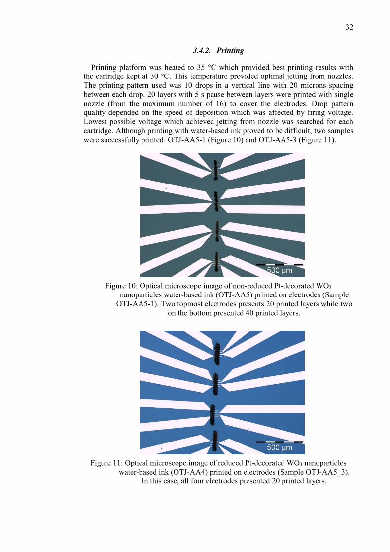
were successfully printed: OTJ-AA5-1 (Figure 10) and OTJ-AA5-3 (Figure 11).

Figure 10: Optical microscope image of non-reduced Pt-decorated WO3

nanoparticles water-based ink (OTJ-AA5) printed on electrodes (Sample

OTJ-AA5-1). Two topmost electrodes presents 20 printed layers while two

on the bottom presented 40 printed layers.

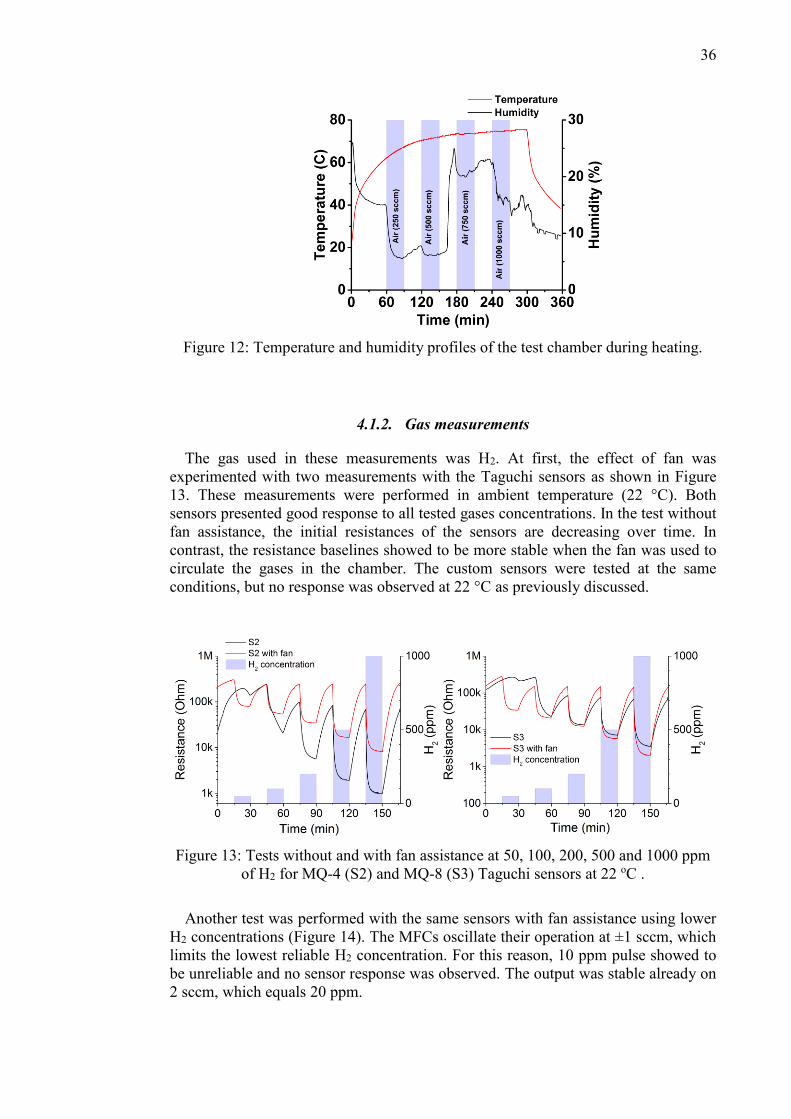
Figure 11: Optical microscope image of reduced Pt-decorated WO3 nanoparticles

water-based ink (OTJ-AA4) printed on electrodes (Sample OTJ-AA5_3).

In this case, all four electrodes presented 20 printed layers.

33

3.4.3. Wire bonding

Due to the inherited design, the chip carrier had contacts for connecting three of the

four electrodes. Therefore, three with lowest resistance values were selected for wire

bonding. In addition, our PCB design ultimately connects them together, so three

sensor structures were connected in parallel hence lowering the initial resistance. The

bonding was made using wire bonding machine (Kulicke & Soffa MODEL 4532)

using 20 µm gold wire. (Kulicke & Soffa) (Picture 16) Picture 17 shows wire

bonding in process.

Picture 16. K&S MODEL 4543 wire bonding machine.

Picture 17: Wire bonding in process.

34

3.5. Test chamber

The body and the ports of the acid-proof stainless steel chamber was welded

together with tungsten inert gas (TIG) welding and a polytetrafluoroethylene (PFTE)

ring was made to seal the chamber at normal pressure conditions. The chamber was

connected to gas flow system with 6 mm pipes. A 15-pin serial feedthrough from

Allectra was used to transmit data. A heater block was constructed using 40 W

Kapton® heater foil between aluminium heat sinks and the attached fan. Heater

resistor and fan were powered with the serial cable. The heater block assembly is

shown in Picture 18. Complete assembly of the calibration setup is shown in Picture

19.

Picture 18: Heater block with fan.

Picture 19: An operational calibration measurement setup in test chamber before

fastening the lid.

35

4. RESULTS

4.1. Measurements

The test chamber was attached to a gas measurement system which has multiple

gases available. For measurements synthetic air (AGA, 80% nitrogen (N2), 20%

oxygen (O2)) and hydrogen (AGA, 99 % N2, 1% H2) was used. Gas flow was

regulated by an array of mass flow controllers (MFC), (MKS Instruments 1179A

Mass-Flo®, 1-1000 sccm flow rate) attached to a PC. The gas flow profiles and the

measurement system were controlled with a custom LabVIEW program. The sensor

board was inserted inside the chamber with the heater block. The DB15 serial

feedthrough flange was used to transmit data and power to the measurement system,

heater and fan. The YÚN system was connected to the serial cable and it logged the

measurements to a microSD card. The load resistances were adjusted with trimmer

potentiometers as close as possible to 50 kΩ for Taguchi sensors and 5 MΩ for

custom fabricated sensors in order to ensure optimal range for ADC operation. Exact

resistance values were inserted in the calibration program to calculate accurate sensor

resistances from raw ADC data.

Commercial methane (CH4) sensitive MQ-4 and a hydrogen (H2) sensitive MQ-8

Taguchi-type sensors were chosen as reference sensors. According to their positions

on the board sensor they were denominated as S2 and S3, respectively. Also the two

inkjet-printed sensors, OTJ-AA5-1 (S1) and OTJ-AA5-3 (S4) were measured.

4.1.1. Thermal profiling

The initial measurements at ambient temperature of 22 °C showed no response from

custom sensors which was expectable result since most of the studies utilizing WO3

as gas sensor described response at temperatures from 70 to 300 °C [2], [21], [23],

[30]. For this reason, a heater block was attached to the system to enhance

sensitivity. The maximum specified power was achieved with a power supply

(EL302 power supply, 30 V / 2 A, Thurlby-Thandar Instruments Ltd.) providing 1.41

A at 28.4 V resulting in 40 W. After pre-heating the chamber, synthetic air was

vented through with various flows (250, 500, 750, 1000 sccm).

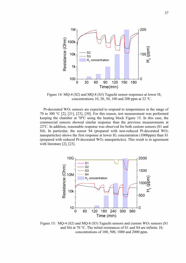
The chamber reaches 60 °C in approximately one hour and 70 °C in two hours as

shown in Figure 12. In addition, once the inner temperature is reached no significant

changes were observed. This result indicates that the air flow does not affect the

temperature during the sensor measurements. The humidity variation is mostly due to

the low humidity (< 10 %) of the synthetic air. There might be also some degassing

and humidity from the inserted components.

36

Figure 12: Temperature and humidity profiles of the test chamber during heating.

4.1.2. Gas measurements

The gas used in these measurements was H2. At first, the effect of fan was

experimented with two measurements with the Taguchi sensors as shown in Figure

13. These measurements were performed in ambient temperature (22 °C). Both

sensors presented good response to all tested gases concentrations. In the test without

fan assistance, the initial resistances of the sensors are decreasing over time. In

contrast, the resistance baselines showed to be more stable when the fan was used to

circulate the gases in the chamber. The custom sensors were tested at the same

conditions, but no response was observed at 22 °C as previously discussed.

Figure 13: Tests without and with fan assistance at 50, 100, 200, 500 and 1000 ppm

of H2 for MQ-4 (S2) and MQ-8 (S3) Taguchi sensors at 22 oC .

Another test was performed with the same sensors with fan assistance using lower

H2 concentrations (Figure 14). The MFCs oscillate their operation at ±1 sccm, which

limits the lowest reliable H2 concentration. For this reason, 10 ppm pulse showed to

be unreliable and no sensor response was observed. The output was stable already on

2 sccm, which equals 20 ppm.

37

Figure 14: MQ-4 (S2) and MQ-8 (S3) Taguchi sensor responses at lower H2

concentrations 10, 20, 50, 100 and 200 ppm at 22 oC.

Pt-decorated WO3 sensors are expected to respond to temperatures in the range of

70 to 300 °C [2], [21], [23], [30]. For this reason, test measurement was performed

keeping the chamber at 70oC using the heating block Figure 15. In this case, the

commercial sensors showed similar response than the previous measurements at

22oC. In addition, reasonable response was observed for both custom sensors (S1 and

S4). In particular, the sensor S4 (prepared with non-reduced Pt-decorated WO3

nanoparticles) shows the first response at lower H2 concentration (1000ppm) than S1

(prepared with reduced Pt-decorated WO3 nanoparticles). This result is in agreement

with literature [2], [23].

Figure 15: MQ-4 (S2) and MQ-8 (S3) Taguchi sensors and custom WO3 sensors (S1

and S4) at 70 °C. The initial resistances of S1 and S4 are infinite. H2

concentrations of 100, 500, 1000 and 2000 ppm.

38

4.2. Device operation

The measuring functionality of the devices was validated by the calibration

measurements as the data was saved to a memory card to be later processed in

Origin. A 2 s refresh rate was used in the calibration measurements. The temperature

values proved to be inaccurate due to a design flaw which placed the sensor too close

to gas sensor’s heater coil.

Besides the calibration measurements performed using Taguchi sensors, the

devices were kept in ambient temperature conditions and operated on several

occasions to validate the data logging and uploading. The sensor data was

successfully logged to the memory cards and shown with digits on YÚN system and

graphically on RPi system.

Cloud functionality was tested by setting up a Dropbox applications for both

systems. A python script ran on the Linux side of YÚN to upload the measurement

file to Dropbox. On Raspberry Pi the python code responsible of the graphical

representation was modified to include the same uploading functionality.

The battery used in RPi system supplied sufficient power to run all the components

including sensor board and display. Contrary to the battery bank’s specifications it

could not power the system up while recharging the battery. In the scope of this

thesis work, the regulators were not used and YÚN system was powered with 5 V

DC supply.

The final weight of the YÙN system is 190 g and 415 g for the RPi system. The

dimensions of the YÚN system are 113x76x60 mm. Total dimensions for RPi system

are 176x75x68 mm with sensor board attached.

The practical side of the design worked as intended. The switching of sensors and

adjusting load resistances was straightforward due to the measurements points on the

middle of sensor board. The stacking and fitting of the boards went as intended. The

operational systems are shown in Picture 20 (YÚN system) and Picture 21 (RPi

system).

39

Picture 20: YÚN system in operation.

Picture 21: Raspberry Pi system in operation.

40

5. CONCLUSIONS

The scope of the thesis was relatively broad, but the subject can be thought to be

comprised of two main focuses: the entity of device, its manufacturing processes and

the fabrication of representative metal oxide gas sensors used to test the system.

Two systems were specified, designed and manufactured. Design flow included

application mapping, schematic and layout drawing, PCB manufacturing and reflow

soldering, manual assembly and 3D-printing of the enclosures. The devices were

programmed to support the components in the system and provide the required

functionality.

In addition, reduced and non-reduced Pt-decorated WO3 nanoparticles were

synthesized. These nanoparticle powders were used in the preparation of water-

based inks for further inkjet printing. A set of sensor chips were fabricated by inkjet

printing onto an electrode structure and wire bonding those chips to chip carriers.

In order to test the device operation, the sensors were tested using H2 in the

manufactured test chamber. Commercial Taguchi sensors showed good response at

22 oC and 70 oC as well as to lower H2 concentrations. In agreement to the literature

[2],[23], custom made Pt-WO3 sensors showed response only at 70 oC and higher H2

concentrations. The device operated as expected and ADC noise was insignificant.

The inaccurate readings of temperature sensor could be easily corrected by

improving the layout design. As one of the motivations for thesis work was to enable

measurements for sample sensors without sophisticated test equipment in laboratory

conditions, a better responding sensor material in room temperatures could have been

chosen. Nonetheless, the functionality of the features could be verified.

The work flows of the thesis were comprehensive overviews of the design

challenges in electrical engineering; both in microelectronics and conventional

electronics design as well as in embedded programming. Starting from the physical

and chemical composition of materials, microelectronics fabrication methods were

discussed. The principles of measurement devices were studied, a CAD -based PCB

design flow was presented and finally the system was programmed from lower level

embedded functions to a GUI running on Linux system and cloud functionality.

The entity of these interlinked design tasks could be considered as a simplified

representation of the value chain endeavoured by the department of electrical

engineering in its entirety. Although superficial on certain aspects, the thesis work

introduced lots of design considerations and interactions between different layers of

the system. As the engineering process of a CPS is unquestionably diverse subject,

it’s beneficial for all participants to have some knowledge from every other segment.

The systems could be further developed to utilize the heater circuits in custom

circuits and adding a low-pass filter to the PWM output. The 10-bit ADC used in the

system could be upgraded to more accurate 12-bit one with only slight modifications

to driver libraries. The system could be used with other kind of sensors besides gas

sensors. The software fulfils the basic requirements and could be improved further.

Although portability requirement was achieved, further miniaturizing and

integrating the system and sensor design could allow it to be equipped on a drone.

This could achieve 3D –plotting of the sensor data in large environments.

41

6. REFERENCES

[1] J. Kukkola, “Gas sensors based on nanostructured tungsten oxides,” The

University of Oulu, 2013.

[2] J. Kukkola, M. Mohl, A.-R. Leino, G. Tóth, M.-C. Wu, A. Shchukarev, A.

Popov, J.-P. Mikkola, J. Lauri, M. Riihimäki, J. Lappalainen, H. Jantunen, and

K. Kordás, “Inkjet-printed gas sensors: metal decorated WO3 nanoparticles

and their gas sensing properties,” J. Mater. Chem., vol. 22, no. 34, p. 17878,

Aug. 2012.

[3] R. Rajkumar, I. Lee, L. Sha, and J. Stankovic, “Cyber-physical systems: the

next computing revolution,” Proc. 47th …, 2010.

[4] P. Marwedel, “Embedded and cyber-physical systems in a nutshell,” DAC.

COM Knowl. Cent. Artic., 2010.

[5] A. Usman and H. Mukhtar, “Design Time Considerations for Cyber Physical

Systems,” in 2012 IEEE International Conference on Green Computing and

Communications, 2012, pp. 442–445.

[6] J. Singh and O. Hussain, “Cyber-Physical Systems as an Enabler for Next

Generation Applications,” in 2012 15th International Conference on Network-

Based Information Systems, 2012, pp. 417–422.

[7] R. Baheti and H. Gill, “Cyber-physical systems,” impact Control Technol.,

2011.

[8] E. A. Lee, “Introducing embedded systems: a cyber-physical approach,” in

Proceedings of the 2009 Workshop on Embedded Systems Education - WESS

’09, 2009, pp. 1–2.

[9] P. Marwedel, Embedded System Design: Embedded Systems Foundations of

Cyber-Physical Systems, vol. 16. Springer Science & Business Media, 2010.

[10] G. Heiland, “Zum Einfluß von adsorbiertem Sauerstoff auf die elektrische

Leitfähigkeit von Zinkoxydkristallen,” Zeitschrift für Phys., 1954.

[11] A. Bielanski, J. Deren, and J. Haber, “Electric conductivity and catalytic

activity of semiconducting oxide catalysts,” Nature, 1957.

[12] T. Siyama and A. Kato, “A new detector for gaseous components using

semiconductor thin film,” Anal. Chem, 1962.

[13] N. BARSAN, D. KOZIEJ, and U. WEIMAR, “Metal oxide-based gas sensor

research: How to?,” Sensors Actuators B Chem., vol. 121, no. 1, pp. 18–35,

Jan. 2007.

[14] P. Shankar and J. Rayappan, “Gas sensing mechanism of metal oxides: The

role of ambient atmosphere, type of semiconductor and gases-A review,”

ScienceJet, 2015.

[15] H. Meixner and U. Lampe, “Metal oxide sensors,” Sensors Actuators B

Chem., vol. 33, no. 1–3, pp. 198–202, Jul. 1996.

[16] C. Wang, L. Yin, L. Zhang, D. Xiang, and R. Gao, “Metal oxide gas sensors:

42

sensitivity and influencing factors.,” Sensors (Basel)., vol. 10, no. 3, pp. 2088–

106, Jan. 2010.

[17] N. Taguchi, “A metal oxide gas sensor,” Japanese Pat., 1962.

[18] S. R. Morrison, “Semiconducting-oxide chemical sensors,” IEEE Circuits

Devices Mag., vol. 7, no. 2, pp. 32–35, Mar. 1991.

[19] N. Yamazoe, G. Sakai, and K. Shimanoe, “Oxide Semiconductor Gas

Sensors,” Catal. Surv. from Asia, vol. 7, no. 1, pp. 63–75.

[20] J. . Solis, S. Saukko, L. Kish, C. . Granqvist, and V. Lantto, “Semiconductor

gas sensors based on nanostructured tungsten oxide,” Thin Solid Films, vol.

391, no. 2, pp. 255–260, Jul. 2001.

[21] S. J. Ippolito, S. Kandasamy, K. Kalantar-zadeh, and W. Wlodarski,

“Hydrogen sensing characteristics of WO3 thin film conductometric sensors

activated by Pt and Au catalysts,” Sensors Actuators B Chem., vol. 108, no. 1–

2, pp. 154–158, Jul. 2005.

[22] M. Takács, C. Dücső, and A. E. Pap, “Fine-tuning of gas sensitivity by

modification of nano-crystalline WO3 layer morphology,” Sensors Actuators

B Chem., vol. 221, pp. 281–289, Dec. 2015.

[23] J. Kukkola, M. Mohl, A.-R. Leino, J. Mäklin, N. Halonen, A. Shchukarev, Z.

Konya, H. Jantunen, and K. Kordas, “Room temperature hydrogen sensors

based on metal decorated WO3 nanowires,” Sensors Actuators B Chem., vol.

186, pp. 90–95, Sep. 2013.

[24] C.-C. Chan, W.-C. Hsu, C.-C. Chang, and C.-S. Hsu, “Preparation and

characterization of gasochromic Pt/WO3 hydrogen sensor by using the

Taguchi design method,” Sensors Actuators B Chem., vol. 145, no. 2, pp. 691–

697, Mar. 2010.

[25] D. Lee, “Nitrogen oxides-sensing characteristics of WO3-based

nanocrystalline thick film gas sensor,” Sensors Actuators B Chem., vol. 60, no.

1, pp. 57–63, Nov. 1999.

[26] W.-C. Hsu, C.-C. Chan, C.-H. Peng, and C.-C. Chang, “Hydrogen sensing

characteristics of an electrodeposited WO3 thin film gasochromic sensor

activated by Pt catalyst,” Thin Solid Films, vol. 516, no. 2–4, pp. 407–411,

Dec. 2007.

[27] P. J. Shaver, “ACTIVATED TUNGSTEN OXIDE GAS DETECTORS,”

Appl. Phys. Lett., vol. 11, no. 8, p. 255, 1967.

[28] J. Kukkola, J. Mäklin, N. Halonen, T. Kyllönen, G. Tóth, M. Szabó, A.

Shchukarev, J.-P. Mikkola, H. Jantunen, and K. Kordás, “Gas sensors based

on anodic tungsten oxide,” Sensors Actuators B Chem., vol. 153, no. 2, pp.

293–300, Apr. 2011.

[29] X.-L. Li, T.-J. Lou, X.-M. Sun, and Y.-D. Li, “Highly Sensitive WO 3

Hollow-Sphere Gas Sensors,” Inorg. Chem., vol. 43, no. 17, pp. 5442–5449,

Aug. 2004.

[30] M. Penza, C. Martucci, and G. Cassano, “NOx gas sensing characteristics of

43

WO3 thin films activated by noble metals (Pd, Pt, Au) layers,” Sensors

Actuators B Chem., vol. 50, no. 1, pp. 52–59, Jul. 1998.

[31] I. Kocemba and T. Paryjczak, “Metal films on a SnO2 surface as selective gas

sensors,” Thin Solid Films, vol. 272, no. 1, pp. 15–17, Jan. 1996.

[32] K. Fujimoto, M. Uchijima, M. Masai, and T. Inui, New Aspects of Spillover

Effect in Catalysis. 1993.

[33] J. Mizsei, P. Sipilä, and V. Lantto, “Structural studies of sputtered noble metal

catalysts on oxide surfaces,” Sensors Actuators B Chem., vol. 47, no. 1–3, pp.

139–144, Apr. 1998.

[34] “Arduino Yun.” Arduino LLC, 2013.

[35] “Raspberry Pi 2 Model B | Raspberry Pi.” Raspberry Pi Foundation, 2015.

[36] Microchip, “2.7V 4-Channel/8-Channel 10-Bit A/D Converters with SPI

Serial Interface.” Microchip, pp. 1–40, 2008.

[37] “MQ-4.” Zhengzhou Winsen Electronic Technology Co., Ltd.

[38] “Flammable Gas Sensor MQ-8.” Zhengzhou Winsen Electronics Technology

Co., Ltd, p. 7, 2014.

[39] T. Liu, “AM2302/DHT22,” pp. 1–5.

[40] Fairchild Semiconductor, “FQP30N06L,” no. November. Fairchild

Semiconductor, pp. 1–9, 2013.

[41] Multicomp, “Power Diodes Power Diodes Ultra-Fast Recovery.” multicomp,

pp. 1–3, 2012.

[42] “ADP2303.” [Online]. Available: http://www.analog.com/media/en/technical-

documentation/data-sheets/ADP2302_2303.pdf. [Accessed: 09-Nov-2015].

[43] “Specification for LCD module.” Huanan Electronic Technology Co., Ltd,

2012.

[44] “LCD Module Specification.” Multi-Inno Technology Co., Ltd, p. 33, 2012.

[45] “MCP3008 Tutorial 02: Sampling DC Voltage - Rheingold HeavyRheingold

Heavy.” [Online]. Available: https://rheingoldheavy.com/mcp3008-tutorial-

02-sampling-dc-voltage/. [Accessed: 23-Sep-2015].

[46] A. Daftery, “Ankit D’s Space -> Dropbox Datalogger,” 2014. [Online].

Available: http://ankitdaf.com/projects/DropboxDatalogger/. [Accessed: 26-

Feb-2016].

[47] “PyQtGraph - Scientific Graphics and GUI Library for Python.” [Online].

Available: http://pyqtgraph.org/. [Accessed: 26-Feb-2016].

[48] A. Fabrizi, “BASH Dropbox Uploader.” [Online]. Available:

https://www.andreafabrizi.it/?dropbox_uploader. [Accessed: 26-Feb-2016].

44

7. APPENDICES

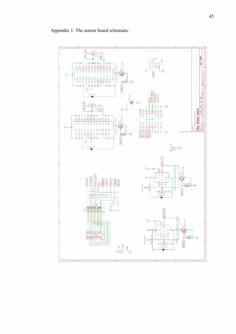
Appendix 1: The sensor board schematic

Appendix 2: Arduino YÚN interface board schematic

Appendix 3: Raspberry Pi interface board schematic

Appendix 4: Test chamber design drawing

Appendix 5: YÚN main program (YUN_final.ino)

Appendix 6: adc.h library (adc.h and adc.cpp)

Appendix 7: tft_ui.h library (tft_ui.h and tft_ui.cpp)

Appendix 8: Python program for Raspberry Pi (sgs5.py)

45

Appendix 1: The sensor board schematic

46

Appendix 2: Arduino YÚN interface board schematic

47

Appendix 3: Raspberry Pi interface board schematic

48

Appendix 4: Test chamber design drawing

49

Appendix 5: YÚN main program (YUN_final.ino)

// Main program for the YUN system. ADC and TFT control are included as libraries. Python script and timestamp function from // https://github.com/ankitdaf/yun-datalogger-dropbox/blob/master/LogToDropbox/LogToDropbox.ino // tft_ui.h written by me. // Topias Jarvinen 2016-02-23 #include <SPI.h> // Include the SPI library #include <TFT.h> // Arduino LCD library #include <DHT.h> // DHT temp/humidity sensor library #include <adc.h> // ADC conversion library #include <tft_ui.h> // TFT draw library #include <FileIO.h> // File operations library #include <Process.h> // Process library for Linux side communication #define DHTPIN 8 // DHT sensor pin #define DHTTYPE DHT22 // DHT sensor type long previousMillis = 0; // Millisecond variable for timing temperature readings long interval = 10000; // Temperature reading interval float temp = 0; // Temperature variable float humidity = 0; // Humidity variable float corr = 0; // Resistance correction factor float VH1_to_4[4] = 0, 5000, 5000, 0; // Sensors 1-4 heater voltages in mV float RL1_to_4[4] = 5000000, 50000, 50000, 5000000; // Sensors 1-4 load resistance in Ohms const int CS_MCP3008 = 4; // ADC Chip Select pin const int CS_TFT = 7; // TFT Chip Select pin tft_ui tft_ui(CS_TFT); // TFT library initialization DHT dht(DHTPIN, DHTTYPE); // DHT library uinitialization adc adc(CS_MCP3008); // ADC library initialization float CH0_to_3 [4]; // Array for ADC values float RS1_to_4 [4]; // Array for resistance values void setup() Bridge.begin(); // Linux-side bridge SPI.begin (); // SPI bus dht.begin (); // DHT sensor Serial.begin(9600); // Serial tft_ui.init(); // TFT initialization FileSystem.begin(); // SD card filesystem init //PWM PINS SETUP pinMode(3, OUTPUT); // PWM_S1 initialization pinMode(5, OUTPUT); // PWM_S2 initialization pinMode(9, OUTPUT); // PWM_S3 initialization pinMode(10, OUTPUT); // PWM_S4 initialization //pinMode(2, OUTPUT); // Beeper for (int i = 0; i < 4; i++) // Get PWM value from defined heater voltages VH1_to_4[i] = (VH1_to_4[i] / 5000) * 255; analogWrite(3, VH1_to_4[0]); // PWM_S1 voltage analogWrite(5, VH1_to_4[1]); // PWM_S2 voltage analogWrite(9, VH1_to_4[2]); // PWM_S3 voltage analogWrite(10, VH1_to_4[3]); // PWM_S4 voltage Serial.println("copy"); // initialization copy message for debugging purposes

50

void loop() int adc_channel; // For selecting ADC channel int adc_reading; // For storing current ADC reading String dataString; // All writing data as string // Read ADC, temperature and humidity data according to refresh rate unsigned long currentMillis = millis(); if (currentMillis - previousMillis > interval) previousMillis = currentMillis; dataString += getTimeStamp(); dataString += ": "; //Loop all ADC channels and save values to array CH0_to_3 for (adc_channel = 0; adc_channel < 4; adc_channel++) adc_reading = adc.readADC(adc_channel); CH0_to_3 [adc_channel] = adc_reading; dataString += (" Sensor resistances (S1-S4): "); for (int i = 0; i < 4; i++) RS1_to_4[i] = (RL1_to_4[i] * ((1023 / CH0_to_3[i]) - 1)); dataString += (RS1_to_4[i]); dataString += (" "); //Read DHT22 temp = dht.readTemperature(); humidity = dht.readHumidity(); dataString += (" T (C): "); dataString += (temp); dataString += (" H (%): "); dataString += (humidity); // Correction factor debugging corr = THcomp(temp, humidity); dataString += (" Correction factor: "); dataString += (corr); File dataFile = FileSystem.open("/mnt/sd/datalog.txt", FILE_APPEND); dataFile.println(dataString); Serial.println(dataString); dataFile.close(); Process upload; upload.runShellCommand("python /mnt/sda1/arduino/log.py /mnt/sda1/datalog.txt"); // Run the Python script for file upload // Update values on TFT tft_ui.draw(RS1_to_4, temp, humidity); // Optional warning buzzer operation //if (RS1_to_4[1] > 50000) // digitalWrite(2, HIGH); //else // digitalWrite(2, LOW); //delay(3000); // This function calculates the correction factor according to temperature and humidity float THcomp(float temp, float humidity)

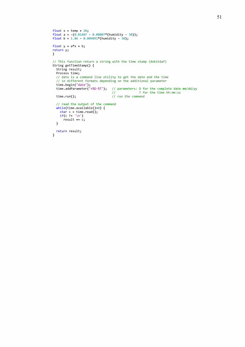
51

float x = temp + 20; float a = -(0.01407 - 0.00007*(humidity - 30)); float b = 1.86 - 0.009091*(humidity - 30); float y = a*x + b; return y; // This function return a string with the time stamp (Ankitdaf) String getTimeStamp() String result; Process time; // date is a command line utility to get the date and the time // in different formats depending on the additional parameter time.begin("date"); time.addParameter("+%D-%T"); // parameters: D for the complete date mm/dd/yy // T for the time hh:mm:ss time.run(); // run the command // read the output of the command while(time.available()>0) char c = time.read(); if(c != '\n') result += c; return result;

52

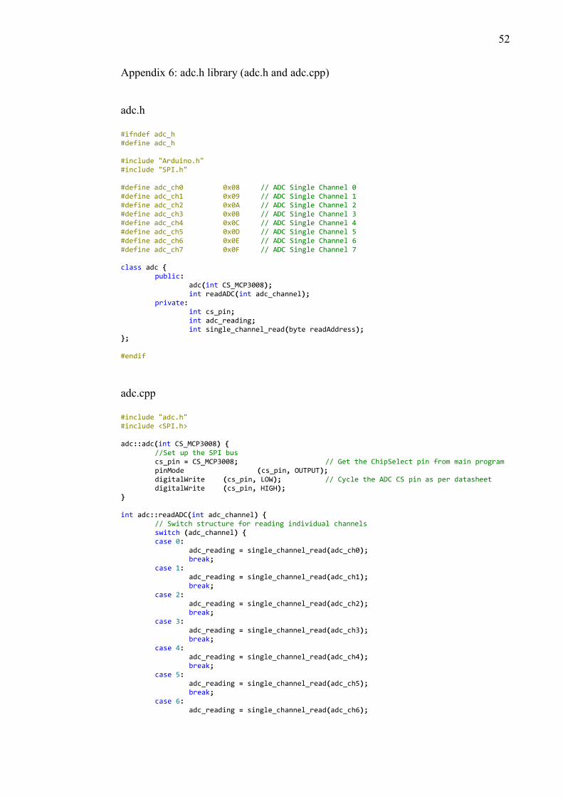
Appendix 6: adc.h library (adc.h and adc.cpp)

adc.h

#ifndef adc_h #define adc_h #include "Arduino.h" #include "SPI.h" #define adc_ch0 0x08 // ADC Single Channel 0 #define adc_ch1 0x09 // ADC Single Channel 1 #define adc_ch2 0x0A // ADC Single Channel 2 #define adc_ch3 0x0B // ADC Single Channel 3 #define adc_ch4 0x0C // ADC Single Channel 4 #define adc_ch5 0x0D // ADC Single Channel 5 #define adc_ch6 0x0E // ADC Single Channel 6 #define adc_ch7 0x0F // ADC Single Channel 7 class adc public: adc(int CS_MCP3008); int readADC(int adc_channel); private: int cs_pin; int adc_reading; int single_channel_read(byte readAddress); ; #endif

adc.cpp

#include "adc.h" #include <SPI.h> adc::adc(int CS_MCP3008) //Set up the SPI bus cs_pin = CS_MCP3008; // Get the ChipSelect pin from main program pinMode (cs_pin, OUTPUT); digitalWrite (cs_pin, LOW); // Cycle the ADC CS pin as per datasheet digitalWrite (cs_pin, HIGH); int adc::readADC(int adc_channel) // Switch structure for reading individual channels switch (adc_channel) case 0: adc_reading = single_channel_read(adc_ch0); break; case 1: adc_reading = single_channel_read(adc_ch1); break; case 2: adc_reading = single_channel_read(adc_ch2); break; case 3: adc_reading = single_channel_read(adc_ch3); break; case 4: adc_reading = single_channel_read(adc_ch4); break; case 5: adc_reading = single_channel_read(adc_ch5); break; case 6: adc_reading = single_channel_read(adc_ch6);

53

break; case 7: adc_reading = single_channel_read(adc_ch7); break; return adc_reading; int adc::single_channel_read(byte readAddress) //Function for reading a single channel byte dataMSB = 0; byte dataLSB = 0; byte JUNK = 0x00; SPI.beginTransaction (SPISettings(2000000, MSBFIRST, SPI_MODE0)); digitalWrite (cs_pin, LOW); SPI.transfer (0x01); // Start Bit dataMSB = SPI.transfer(readAddress << 4) & 0x03; // Send readAddress and receive MSB data, masked to two bits dataLSB = SPI.transfer(JUNK); // Push junk data and get LSB byte return digitalWrite (cs_pin, HIGH); SPI.endTransaction (); return dataMSB << 8 | dataLSB;

54

Appendix 7: tft_ui.h library (tft_ui.h and tft_ui.cpp)

tft_ui.h

#ifndef tft_ui_h #define tft_ui_h #include "Arduino.h" #include "SPI.h" #include "TFT.h" // Define TFT pins. #define cs 7 #define dc 12 #define rst 13 class tft_ui // Define variables public: tft_ui(int CS_TFT); void init(); void draw(float adc_array[], float t, float h); private: float temp; float humidity; float sensorVal_old[4]; float temp_old; float humidity_old; char sensor1Printout[6]; char sensor2Printout[6]; char sensor3Printout[6]; char sensor4Printout[6]; char tempValPrintout[6]; char humidityValPrintout[6]; String sensor1Val; String sensor2Val; String sensor3Val; String sensor4Val; String tempVal; String humidityVal; int xPos; int cs_pin; long value; ; #endif

tft_ui.cpp

#include <TFT.h> #include <SPI.h> #include <tft_ui.h> TFT TFTscreen = TFT(cs, dc, rst); tft_ui::tft_ui(int CS_TFT) cs_pin = CS_TFT; TFT TFTscreen = TFT(cs_pin, dc, rst); void tft_ui::init() TFTscreen.begin(); // initialize tft

55

TFTscreen.background(0, 0, 0); // clear the screen with a black background TFTscreen.stroke(255, 255, 255); // set the font color to white TFTscreen.setTextSize(1); // Write tft texts TFTscreen.text("Sensor Values:\n ", 0, 0); TFTscreen.setTextSize(2); TFTscreen.text(" Ohms", 80, 15); TFTscreen.text(" Ohms", 80, 35); TFTscreen.text(" Ohms", 80, 55); TFTscreen.text(" Ohms", 80, 75); TFTscreen.text(" C", 80, 95); TFTscreen.text(" %RH", 80, 115); void tft_ui::draw(float adc_array[], float temp, float humidity) if(adc_array[0] != sensorVal_old[0]) //If value changes, TFTscreen.stroke(0, 0, 0); //set text color to black, sensor1Val.toCharArray(sensor1Printout, 6); //Read old value to chararray, TFTscreen.text(sensor1Printout, 0, 15); //Print old value in black, sensor1Val = String(adc_array[0]); //Read new value from main program, sensor1Val.toCharArray(sensor1Printout, 6); //send it to chararray, TFTscreen.stroke(255, 255, 255); //set color to white, TFTscreen.text(sensor1Printout, 0, 15); //Print new value. sensorVal_old[0] = adc_array[0]; //Set new value as old if(adc_array[1] != sensorVal_old[1]) TFTscreen.stroke(0, 0, 0); sensor2Val.toCharArray(sensor2Printout, 6); TFTscreen.text(sensor2Printout, 0, 35); sensor2Val = String(adc_array[1]); sensor2Val.toCharArray(sensor2Printout, 6); TFTscreen.stroke(255, 255, 255); TFTscreen.text(sensor2Printout, 0, 35); sensorVal_old[1] = adc_array[1]; if(adc_array[2] != sensorVal_old[2]) TFTscreen.stroke(0, 0, 0); sensor3Val.toCharArray(sensor3Printout, 6); TFTscreen.text(sensor3Printout, 0, 55); sensor3Val = String(adc_array[2]); sensor3Val.toCharArray(sensor3Printout, 6); TFTscreen.stroke(255, 255, 255); TFTscreen.text(sensor3Printout, 0, 55); sensorVal_old[2] = adc_array[2]; if(adc_array[3] != sensorVal_old[3]) TFTscreen.stroke(0, 0, 0); sensor4Val.toCharArray(sensor4Printout, 6); TFTscreen.text(sensor4Printout, 0, 75); sensor4Val = String(adc_array[3]); sensor4Val.toCharArray(sensor4Printout, 6); TFTscreen.stroke(255, 255, 255); TFTscreen.text(sensor4Printout, 0, 75); sensorVal_old[3] = adc_array[3]; if(temp != temp_old) TFTscreen.stroke(0, 0, 0); tempVal.toCharArray(tempValPrintout, 6); TFTscreen.text(tempValPrintout, 0, 95); tempVal = String(temp); tempVal.toCharArray(tempValPrintout, 6); TFTscreen.stroke(255, 255, 255); TFTscreen.text(tempValPrintout, 0, 95); temp_old = temp; if(humidity != humidity_old) TFTscreen.stroke(0, 0, 0); humidityVal.toCharArray(humidityValPrintout, 6); TFTscreen.text(humidityValPrintout, 0, 115); humidityVal = String(humidity);

56

humidityVal.toCharArray(humidityValPrintout, 6); TFTscreen.stroke(255, 255, 255); TFTscreen.text(humidityValPrintout, 0, 115); humidity_old = humidity;

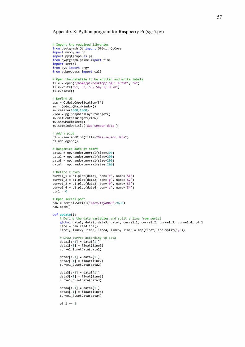
57

Appendix 8: Python program for Raspberry Pi (sgs5.py)

# Import the required libraries from pyqtgraph.Qt import QtGui, QtCore import numpy as np import pyqtgraph as pg from pyqtgraph.ptime import time import serial from sys import argv from subprocess import call # Open the datafile to be written and write labels file = open("/home/pi/Desktop/logfile.txt", "w") file.write("S1, S2, S3, S4, T, H \n") file.close() # Define UI app = QtGui.QApplication([]) mw = QtGui.QMainWindow() mw.resize(1000,1000) view = pg.GraphicsLayoutWidget() mw.setCentralWidget(view) mw.showMaximized() mw.setWindowTitle('Gas sensor data') # Add a plot p1 = view.addPlot(title="Gas sensor data") p1.addLegend() # Randomize data at start data1 = np.random.normal(size=200) data2 = np.random.normal(size=200) data3 = np.random.normal(size=200) data4 = np.random.normal(size=200) # Define curves curve1_1 = p1.plot(data1, pen='r', name='S1') curve1_2 = p1.plot(data2, pen='g', name='S2') curve1_3 = p1.plot(data3, pen='b', name='S3') curve1_4 = p1.plot(data4, pen='c', name='S4') ptr1 = 0 # Open serial port raw = serial.Serial("/dev/ttyAMA0",9600) raw.open() def update(): # Define the data variables and split a line from serial global data1, data2, data3, data4, curve1_1, curve1_2, curve1_3, curve1_4, ptr1 line = raw.readline() line1, line2, line3, line4, line5, line6 = map(float,line.split(",")) # Draw curves according to data data1[:-1] = data1[1:] data1[-1] = float(line1) curve1_1.setData(data1) data2[:-1] = data2[1:] data2[-1] = float(line2) curve1_2.setData(data2) data3[:-1] = data3[1:] data3[-1] = float(line3) curve1_3.setData(data3) data4[:-1] = data4[1:] data4[-1] = float(line4) curve1_4.setData(data4) ptr1 += 1

58

# Open file for appending data file = open("/home/pi/Desktop/logfile.txt", "a") file.write(line) file.close() # Upload the datafile to Dropbox with the dropbox_uploader script ufile = "/home/pi/Dropbox-Uploader/dropbox_uploader.sh upload /home/pi/Desktop/logfile.txt logfile.txt" call ([ufile], shell=True) # Timer for refresh rate timer = QtCore.QTimer() timer.timeout.connect(update) timer.start(5000) if __name__ == '__main__': import sys if (sys.flags.interactive != 1) or not hasattr(QtCore, 'PYQT_VERSION'): QtGui.QApplication.instance().exec_()