Master’s Thesis Extracting Information on Trafﬁc Changes ...

Master’s Thesis

Title

Extracting Information on Traffic Changes from Social Media Data

for Predictive Traffic Engineering

Supervisor

Professor Masayuki Murata

Author

Kota Kawashima

February 6th, 2017

Department of Information Networking

Graduate School of Information Science and Technology

Osaka University

Master’s Thesis

Extracting Information on Traffic Changes from Social Media Data for Predictive Traffic

Engineering

Kota Kawashima

Abstract

The amount of traffic through networks is increasing both in quantity and in fluctuation as

the mobile terminals such as smartphones and tablets become popular. The network must accom-

modate such fluctuating traffic without degrading the network performance. We have proposed a

predictive traffic engineering (TE), based on Model Predictive Control (MPC). MPC is a method

of process control using the prediction of the dynamics of the system. Our predictive TE method

gradually changes the placements of the VNFs, considering the predicted future traffic. By grad-

ually changing the placements, this method allocates required resources in advance based on the

predicted traffic. As a result, the degradation of the network performance is avoided. However,

the accuracy of the predicted traffic has the large impacts on the predictive network control; if the

prediction is inaccurate, our method cannot allocate the network resources in advance. The events

in the real world may cause such traffic changes; during the event in the real world, many partic-

ipants may concentrate at the area, which leads to the increase of the network demands from the

area. As the sophisticated mobile terminals become popular, the impacts of the events in the real

world on the network traffic become large. Therefore, detecting the sign of such traffic changes

and predicting them caused by events in the real world are important problems.

In this thesis, we investigate the signs of traffic changes caused by events in the real world

included in the social media data. We use tweets obtained from Twitter API as the social media

data. We first propose a method that extracts the words related to real-word events from tweets.

Then, we hypothesized that the increase of the number of tweets including extracted words is one

of the signs of the unusual traffic changes. Based on this hypothesis, we propose a method that

forecasts the unusual traffic increase caused by the real-world events from tweets. Our method

forecasts the unusual traffic increase by the following steps; (1) our method extracts the words

1

from tweets, (2) counts the number of tweets including the extracted words in the current and

previous time, (3) predicts the number of the tweets including the words at the next time from

the number of tweets including in the current and previous time and (4) forecasts based on the

predicted number of tweets.

We investigate the accuracy of the forecast. The results show that the method based on the

social media data forecasts the future unusual traffic change accurately; the method based on the

social media data achieves the false negative rate less than 0.1 with the false positive rate less

than 0.49. The results indicate that the words related to the real-world events are the signs of the

unusual traffic changes, and are useful as the input of the future traffic prediction.

Keywords

Traffic Engineering

Traffic Prediction

Forecasting Unusual Traffic Changes

Social Media Data

Twitter

2

Contents

1 Introduction 7

2 Related Work 10

2.1 Dynamic Network Control . . . . . . . . . . . . . . . . . . . . . . . . . . . . . 10

2.2 Traffic Prediction . . . . . . . . . . . . . . . . . . . . . . . . . . . . . . . . . . 11

2.3 Data Mining for Social Media . . . . . . . . . . . . . . . . . . . . . . . . . . . 12

3 Predictive Traffic Engineering 13

3.1 Network Function Virtualization . . . . . . . . . . . . . . . . . . . . . . . . . . 13

3.2 Predictive Traffic Engineering to Place Virtual Network Functions . . . . . . . . 13

3.2.1 Network Model . . . . . . . . . . . . . . . . . . . . . . . . . . . . . . . 14

3.2.2 Overview of Model Predictive Control . . . . . . . . . . . . . . . . . . . 16

3.2.3 Placement of Virtual Network Functions based on Model Predictive Control 16

3.3 Effectiveness of Predictive Traffic Engineering . . . . . . . . . . . . . . . . . . 17

4 Extracting Information on Traffic Changes from Social Media Data 20

4.1 Overview of Social Media Data . . . . . . . . . . . . . . . . . . . . . . . . . . 20

4.2 Extracting Words related to Real-World Events . . . . . . . . . . . . . . . . . . 20

4.2.1 Overview of Term Frequency Inverse Document Frequency . . . . . . . 21

4.2.2 Applying TFIDF to Social Media Data . . . . . . . . . . . . . . . . . . 21

4.3 Forecasting Unusual Traffic Changes based on Extracted Words . . . . . . . . . 23

5 Evaluation 25

5.1 Evaluation Methodology . . . . . . . . . . . . . . . . . . . . . . . . . . . . . . 25

5.1.1 Definition of Unusual Traffic Changes . . . . . . . . . . . . . . . . . . . 25

5.1.2 Parameter Setting . . . . . . . . . . . . . . . . . . . . . . . . . . . . . . 26

5.1.3 Datasets . . . . . . . . . . . . . . . . . . . . . . . . . . . . . . . . . . . 26

5.1.4 Compared Method . . . . . . . . . . . . . . . . . . . . . . . . . . . . . 27

5.1.5 Metrics . . . . . . . . . . . . . . . . . . . . . . . . . . . . . . . . . . . 30

5.2 Evaluation Result . . . . . . . . . . . . . . . . . . . . . . . . . . . . . . . . . . 30

5.3 Discussion . . . . . . . . . . . . . . . . . . . . . . . . . . . . . . . . . . . . . . 35

3

6 Conclusion 36

Acknowledgements 37

References 38

Appendix A Optimization Problem of MPC-VNF-P 41

4

List of Figures

1 Physical network . . . . . . . . . . . . . . . . . . . . . . . . . . . . . . . . . . 14

2 Service chain . . . . . . . . . . . . . . . . . . . . . . . . . . . . . . . . . . . . 15

3 Overview of MPC. . . . . . . . . . . . . . . . . . . . . . . . . . . . . . . . . . 16

4 Overview of MPC-VNF-P. . . . . . . . . . . . . . . . . . . . . . . . . . . . . . 16

5 The network topology . . . . . . . . . . . . . . . . . . . . . . . . . . . . . . . . 18

6 Maximum Accommodation Rate . . . . . . . . . . . . . . . . . . . . . . . . . . 19

7 FNR and FPR (ϵ = 80, Shibuya station) . . . . . . . . . . . . . . . . . . . . . . 30




11 FNR and FPR (ϵ = 60, Namba station) . . . . . . . . . . . . . . . . . . . . . . . 34

12 FNR and FPR (ϵ = 50, Namba station) . . . . . . . . . . . . . . . . . . . . . . . 35

5

List of Tables

1 Average of tweets at time of day (Shibuya station) . . . . . . . . . . . . . . . . . 28

2 Average of tweets at time of day (Namba station) . . . . . . . . . . . . . . . . . 29

6

1 Introduction

As the terminals such as smartphones and tables become popular, the amount of traffic through

the network is increasing both in quantity and in fluctuation. Network service providers require

to handle such large traffic fluctuations without degrading communication quality. So far, this

problem is addressed by preparing redundant resources to accommodate not only the average

traffic but also traffic surge. However, this method requires higher costs, as the traffic fluctuation

becomes large.

Therefore, methods to control networks dynamically have been proposed [1–3]. These meth-

ods dynamically allocate the network resources, following to the traffic changes. The network

function virtualization (NFV) [4] enables the dynamic placement of the network functions such as

routers, firewall and so on. Therefore, the methods to control the locations of the network func-

tions following to the traffic changes have also been proposed. By dynamically controlling the

locations of the network functions and allocating more resources to the network functions whose

demands are large, these methods handle traffic changes without degrading the performance.

Most of the methods that dynamically control network resources use the observed network

traffic. However, the control based on the observed traffic has the following problems. (1) The

configured resource allocation does not suit the actual traffic when significant traffic change oc-

curs, but the configured resource allocation is not changed until the next control cycle. (2) The

necessity of reconfiguration of the resource allocation may not be detected before the problem

occurs. As a result, significant changes of resource allocations may be required.

Therefore, we have proposed a predictive traffic engineering method [5]. This method grad-

ually changes the placements of the VNFs, considering the predicted future traffic. By gradually

changing the placements, this method handles the traffic changes without requiring the significant

changes of the placements. In addition, this method allocates required resources in advance based

on the predicted traffic. As a result, the degradation of the network performance is avoided. How-

ever, the accuracy of the predicted traffic has the large impacts on the predictive network control;

if the prediction is inaccurate, the predictive network control cannot allocate the network resources

in advance.

Many methods to predict network traffic have been proposed [6–8]. These methods model

the traffic changes, and their parameters are estimated from the previously observed traffic. Then,

7

the future traffic is predicted from the model. However, these methods cannot follow the traffic

changes whose signs are not included in the previously observed traffic. The events in the real

world may cause such traffic changes; during the event in the real world, many participants may

concentrate at the area, which leads to the increase of the network demands from the area. As

the sophisticated mobile terminals become popular, the impacts of events in the real world on the

network traffic become large. Therefore, detecting the sign of such traffic changes and predicting

them caused by events in the real world are important problems.

The signs of the events in the real world may be included in social media data. Along with the

popularization of sophisticated mobile terminals, social media service has grown remarkably, and

stores various data on behaviors of people. In recent years, many studies using the data obtained

from the social media are being conducted in the filed such as traffic event detection [9] and

unusual crowd detection [10].

In this thesis, we investigate the signs of traffic changes caused by events in the real world

included in the social media data. We use tweets obtained from Twitter API as the social media

data. We first propose a method that extracts the words related to real-word events from tweets.

Then, we hypothesized that the increase of the number of tweets including extracted words is one

of the signs of the unusual traffic changes. Based on this hypothesis, we propose a method that

forecasts the unusual traffic increase caused by the real-world events from tweets. Our method

forecasts the unusual traffic increase by the following steps; (1) our method extracts the words

from tweets, (2) counts the number of tweets including the extracted words in the current and

previous time, (3) predicts the number of the tweets including the words at the next time from

the number of tweets including in the current and previous time and (4) forecasts based on the

predicted number of tweets.

We investigate the accuracy of the forecast by our method, and demonstrate that method ana-

lyzing the tweets accurately forecast the unusual traffic increases, compared with the method using

only the past traffic rates. Finally, based on the results, we discuss the signs of the traffic changes

caused by events in the real world. The results indicate that the signs of the unusual traffic changes

are included in social media data.

The rest of this thesis is organized as follows. Section 2 explains the related work. Section

3 introduces the predictive traffic engineering that we have proposed. Section 4 describes our

method to forecast the unusual traffic changes. Section 5 evaluates our method to forecast the

8

unusual traffic changes, and discusses the sings of the unusual traffic changes included in the

social media data. Section 6 concludes this thesis.

9

2 Related Work

2.1 Dynamic Network Control

The time variation of the Internet traffic has been increasing. Backbone networks must accom-

modate such time-varying traffic. Methods to control network dynamically have been studied as

approach to handling such time variations efficiently. These methods dynamically allocate the

network resources, following to the traffic changes without degrading the communication quality.

Jiang et al. proposed a network control method to improve resource utilization in data centers’

networks [1]. This method solves the optimization problem considering both of the location of

virtual machines (VMs) which processes traffic and the route which traffic flows.

Dynamic network control to reduce the energy consumption has also been proposed. Abou-

zeid et al. proposed a network control method that reduces the power consumption without violat-

ing the communication quality required by the users [2]. This method calculates the base stations

that must be turned on, based on the predicted traffic demands. Then, by turning off the unneces-

sary base stations, this method reduces the power consumption. Beloglazov et al. also proposed

a method that reduces the power consumption [3]. In this method, the VMs that are hosted by a

server are migrated to another server to reduce the power consumption if the migration enables to

sleep the server.

In recent years, the network virtualization technologies enable the dynamic control of the

placement of the network functions [4]. In the network function virtualization (NFV), the network

functions such as routers and firewalls are virtualized. The virtual network functions (VNFs)

are hosted by ordinary server computers. The network services are provided through the virtual

network constructed of the VNFs. By dynamically placing the VNFs to the suitable server, the

network services are provided without wasting the resources; the VNFs are hosted by a small

number of servers when the demand is small and each VNF requires only small resources. If the

demand increases and more resources become required, the VNFs are migrated to new servers

[11].

Several methods to control the placement of VNFs have been proposed [11–13]. Most of them

are reactive control. That is, they change the placement of VNFs based on the monitored traffic.

However, the control based on the observed traffic has the following problems. (1) The configured

resource allocation does not suit the actual traffic when significant traffic change occurs, but the

10

configured resource allocation is not changed until the next control cycle. (2) The necessity of

reconfiguration of the resource allocation may not be detected before the problem occurs. As a

result, significant changes of resource allocations may be required.

Therefore, we have proposed predictive traffic engineering methods [5]. This method gradu-

ally changes the placements of the VNFs, considering the predicted future traffic. By gradually

changing the placements, this method handles the traffic changes without requiring the significant

changes of the placements. In addition, this method allocates required resources in advance based

on the predicted traffic. As a result, the degradation of the network performance is avoided. The

details of the method are described in Section 3

2.2 Traffic Prediction

The predictive network control requires the prediction of the network traffic. In this subsection,

we introduce the existing methods to predict the network traffic.

Many methods to predict network traffic have been proposed [6–8]. These methods model the

traffic changes, and their parameters are estimated from the previously observed traffic. Then, the

future traffic is predicted from the model.

Liu et al. proposed a traffic prediction method which decomposes the traffic into trend part

and fluctuation part independently [6]. The trend part is predicted by a method with principal

component analysis. The fluctuation part is predicted by ARIMA. Hag et al. clarified that time

series analysis model such as ARIMA is inadequate to apply to traffic prediction due to the Internet

traffic characteristics such as self-similarity and long-range dependence [7]. As a method to solve

the problem, Hag et al. proposed a new prediction model based on ARIMA model that can predict

the traffic at millisecond time scales. Krithikaivasan et al. also proposed an ARCH-based traffic

prediction which can predict the traffic at second time scales [8].

However, these methods cannot follow the traffic changes whose signs are not included in the

previously observed traffic. As a result, predictive network control cannot allocate the required

resources due to the prediction errors. The events in the real world may cause such traffic changes;

during the event in the real world, many participants may concentrate at the area, which leads to

the increase of the network demands from the area. As the sophisticated mobile terminals become

popular, the impacts of events in the real world on the network traffic become large. Therefore,

the prediction of such traffic changes caused by real-world events is one of the important problem.

11

Traffic changes caused by real-world events are difficult to be predicted from only the previ-

ously monitored traffic rates. Therefore, we need another information used to predict such traffic

changes. In this thesis, we discuss the signs of such traffic changes included in the social media

data.

2.3 Data Mining for Social Media

As the sophisticated mobile terminals such as smartphones and tablets become popular, social

media services such as Twitter and Google+ are also become popular. Through social media, in-

dividuals can easily disseminate information. Therefore, the information on the real-world events

is included in the social media data.

In recent years, many studies using the data obtained from the social media are being con-

ducted. Andrea et al. [9] proposed a method to detect the traffic events such as congestion and

accidents based on the data obtained from Twitter. This method obtains the tweets including the

keywords that are possible to be related to the traffic events. Then, this method assigns the labels

to the tweets. Finally the traffic events are detected by analyzing the labeled tweets.

A method to detect crowds using social media data has also been proposed. Khalifa et al. [10]

indicated that it is possible to detect the presence and size of the crowd by clustering the location

information attached to tweets. Furthermore, they also proposed a method to detect an unusual

crowd by comparing the current crowd with the crowd pattern of normal day.

As demonstrated by these studies, the social media data includes the information on the real-

world events. The unusual changes of the network traffic may be caused by the real-world events.

That is, the social media data may include the sings of the unusual traffic changes caused by the

real-world events, which is investigated in this thesis.

12

3 Predictive Traffic Engineering

We have proposed a predictive traffic engineering method [5]. This method is based on the Net-

work Function Virtualization (NFV). Thus, we explain the overview of the NFV. Then, we explain

the predictive traffic engineering method, and its performance.

3.1 Network Function Virtualization

The network function virtualization (NFV) is one of the promising approaches to accommodat-

ing fluctuating traffic [4]. In the NFV, the network functions such as routers and firewalls are

virtualized. The virtual network functions (VNFs) are hosted by ordinary server computers. The

network services are provided through the virtual network constructed of the VNFs. By dynami-

cally placing the VNFs to the suitable server, the network services are provided without wasting

the resources and energy consumption; the VNFs are hosted by a small number of servers when

the demand is small and each VNF requires only small resources. If the demand increases and

more resources become required, the VNFs are migrated to new servers [11].

Traffic must be processed by the VNFs in an appropriate order. Service chaining is a tech-

nology that controls the order of the VNFs. In service chaining, the VNFs are connected in the

required order, and a chain is created. We call the chain consisted of the VNFs service chain.

The service chain is placed on the physical network. When the traffic which is required to be

handled by the service chain increases, the placement of the VNF is dynamically changed. The

VNFs should be placed considering the required network performance, the power consumption

and the cost. The problem to obtain the suitable place hosting the VNFs can be formulated as the

virtual network embedding problem, and has been investigated in many papers [14–16].

3.2 Predictive Traffic Engineering to Place Virtual Network Functions

In our predictive traffic engineering, we apply the Model Predictive Control (MPC) [17] to the

network control. In this subsection, we explain the network model, the overview of MPC and our

method to place the VNFs based on MPC.

13

3.2.1 Network Model

In our method, we place the service chains on the physical network. This subsection explains the

network model used by the method.

𝑛"resource

𝑈*+, = {100}

𝐵34, = 100

𝑁, = {𝑛6, 𝑛", 𝑛8, 𝑛9}𝐿, = {𝑙6, 𝑙", 𝑙8, 𝑙9, 𝑙<}

𝑅 = 1

𝐵3+, = 100

𝐵3>, = 100

𝐵3?, = 100

𝐵3@, = 100

𝑛6resource𝑈*4, = {0}

𝑛8resource

𝑈*>, = {100}

𝑛9resource𝑈*?, = {0}

Figure 1: Physical network

Physical Network Figure 1 shows a physical network. The physical network is constructed

of physical nodes and physical links. We denote the set of physical nodes by Np, and the set

of physical links by Lp. The physical network is modeled by a weighted directed graph Gp =

(Np, Lp). The bandwidth of the physical link lp ∈ Lp is denoted by Bplp . The resource of the

physical node np ∈ Np is denoted by a vector Upnp , whose number of elements corresponds to

the number of kinds of resources such as CPU and memory. We denote the number of kinds of

resources by R, and ith element of Upnp by upnp,i.

Traffic from users is identified at the ingress of the network, and is relayed to the corresponding

service chain.

Service Chain Figure 2 shows a service chain. The service chain is constructed of the virtual

nodes and virtual links. We denote the set of virtual nodes by Nv, and the set of virtual links by

Lv. The virtual network is modeled by a weighted directed graph Gv = (Nv, Lv).

14

𝑛#Egress

VM𝑟𝑒𝑞𝑢𝑖𝑟𝑒𝑑resource𝑈123 (𝑡) + 𝐷

𝑣:𝑈123 (𝑡) = {40}𝑛:

Ingress

𝐵A2B1 (𝑡)

= 100

𝑁1 = {𝑣:, 𝑣F}𝐿1 = {𝑙:1, 𝑙F1, 𝑙I1}

𝑅 = 1𝐷 = {10}

𝐵AKB1 (𝑡)

= 100𝐵ALB1 (𝑡)

= 100

VM𝑟𝑒𝑞𝑢𝑖𝑟𝑒𝑑𝑟𝑒𝑠𝑜𝑢𝑟𝑐𝑒:𝑈1K3 (𝑡) + 𝐷

𝑣F𝑈1K3 (𝑡) = {40}

Figure 2: Service chain

Each virtual node corresponds to a VNF, and must be mapped to the physical node that has

sufficient resource to run the VNF. We assume that the virtual nodes are placed on the VMs and

the VMs are placed on the physical nodes in the physical network.

Each virtual node nv ∈ Nv requires the resources of the physical node. The required resources

change in time. We denote the resource required by nv at the time slot t by a vector Uvnv(t).

The VMs are placed on the physical nodes. Therefore, as shown in Figure 2, the VM having

the required resources Uvnv(t) requires the resource of the physical node. In addition, each VM

requires the resources of the physical node to place itself. We denote the resources required by a

VM by a vector D, whose number of elements is R. We denote the ith element of D by di.

The virtual link requires the bandwidth. The required bandwidth changes in time. We denote

the bandwidth required by l ∈ Lv at the time slot t by Bvl (t).

nstartl and nend

l indicate the source and destination nodes of the virtual link l ∈ Lv.

A virtual node can be allocated to multiple physical nodes. For example, at time slot t, a

certain virtual node is hosted by a VM running on the physical node n1. At the next time slot

t + 1, the traffic processed by the VM increases and n1 does not have the sufficient resources to

handle the increased traffic. In this case, a new VM which performs the process of the virtual node

can be placed to another physical node n2.

Figure 2 shows a service chain constructed of two virtual nodes and three virtual links. The

ingress and egress nodes of the chain are the physical node. In this example, the ingress and egress

nodes are n1 and n4 in Figure 1.

15

Prediction Optimization System

Feedback : 𝑦 𝑡 + 1

Output𝑦(𝑡 + 1)

Input𝑢(𝑡 + 1)

Calculate inputs 𝑢 𝑡 + 1 ~𝑢 𝑡 + 𝐻

Predicted value𝑏, 𝑡 + 1 ~𝑏,(𝑡 + 𝐻)

MPC controller

Figure 3: Overview of MPC.

PredictionCalculation by a optimization problem

Physical network

Observed value : X 𝑡 + 1

Y(𝑡 + 1)

Calculate the placement of VNFs 𝑌 𝑡 + 1 ~𝑌 𝑡 +𝐻

Predicted value𝑋- 𝑡 + 1 ~𝑋-(𝑡 +𝐻)

MPC-‐‑‒VNF-‐‑‒P controller • The present time slot is 𝑡• 𝐻 is the predictive horizon

Figure 4: Overview of MPC-VNF-P.

3.2.2 Overview of Model Predictive Control

Figure 3 shows a overview of MPC [17]. The MPC controller predicts the operation of system

for the future time slots [t + 1, ...t + H] called predictive horizon where H is the length of the

predictive horizon. Based on the prediction, the controller calculates the inputs for the predictive

horizon. However, the controller implements only the calculated inputs for the next time slots

[t + 1]. Then, the controller observes the output and corrects the prediction, using the output

value. After the correction, the controller recalculates the inputs for the next time slot with the

corrected prediction. Thus, the MPC controller modifies the prediction by using feedback. By

using and modifying the prediction, the MPC achieves a prediction–based control that is robust to

prediction errors.

3.2.3 Placement of Virtual Network Functions based on Model Predictive Control

We apply the MPC to the dynamical placement of the VNFs. We call this method MPC-VNF-P. In

this method, we consider the predicted future values of the required resources. By considering the

16

predicted future values, we can start migration of VMs in advance of the changes of the required

resources. As a result, we can follow the time variation of the required resources at each time slot.

Figure 4 shows an overview of MPC-VNF-P. The MPC-VNF-P controller (1) predicts the

required resources of VNFs and virtual links for each time slot t+k(1 ≤ k ≤ H), (2) calculates the

physical servers hosting the VMs for future H time slots, and (3) places the VNFs and configures

the routes according to the calculated results for the next time slot. Then, at the next time slot,

the controller obtains the new information on the required resources, and performs the above steps

again. By continuing these steps, the MPC-VNF-P controls the locations of the VNFs considering

the future required resources. In addition, even if the prediction errors are included in the predicted

future required resources, the impact of the prediction errors is avoided by correcting the prediction

at each step.

In the MPC-VNF-P, the controller solves the optimization problem to calculates the physical

servers hosting the VMs. The optimization problem is described in Appendix A.

3.3 Effectiveness of Predictive Traffic Engineering

By applying the MPC to the dynamic placement of the VNFs, our method starts migration of VMs

in advance by considering the predicted future demands. As a result, our method allocates suffi-

cient resources to the VNFs even when traffic variation occurs. In this subsection, we demonstrate

that our method handles the time variation of the demands adequately at any time slot.

We use the topology shown in Figure 5 which is based on the backbone network of the Inter-

net 2 [18] . In this topology, only two physical nodes, which are n1 and n2, have the sufficient

resources to place the VNFs. We set the bandwidth of each link to a sufficiently large value to

focus on the impact of the time variation of the resources required by the VNFs. In this simu-

lation, each Origin-Destination flow from the ingress node to the egress node is processed by a

service chain. There is seventy two OD flows in the network of the Internet 2. Therefore, we

accommodate 72 service chains on the above topology. We set the demands of each OD flow

based on the traffic trace which is collected from 12 November 2011 to 18 November 2011 at the

Internet 2 [19].

In the MPC-VNF-P, the network administrator can limit the number of VMs that can be mi-

grated at each time slot. In this subsection, the upper limit of the number of migrated VMs δ is

set to 1 in the simulation, to demonstrate that our method can work properly even if only a small

17

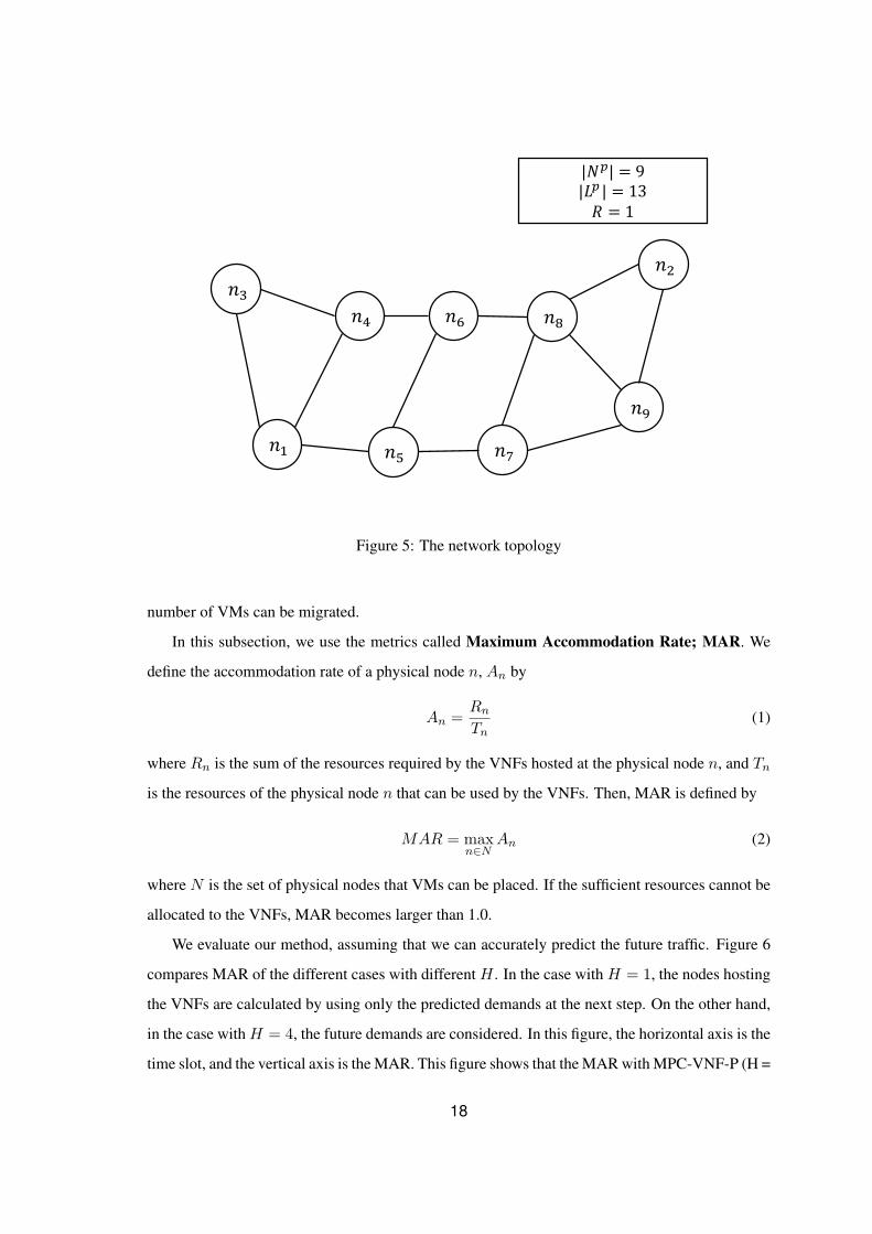
|𝑁#| = 9|𝐿#| = 13𝑅 = 1

𝑛,

𝑛-

𝑛.𝑛/

𝑛0

𝑛1

𝑛2

𝑛3

𝑛4

Figure 5: The network topology

number of VMs can be migrated.

In this subsection, we use the metrics called Maximum Accommodation Rate; MAR. We

define the accommodation rate of a physical node n, An by

An =Rn

Tn(1)

where Rn is the sum of the resources required by the VNFs hosted at the physical node n, and Tn

is the resources of the physical node n that can be used by the VNFs. Then, MAR is defined by

MAR = maxn∈N

An (2)

where N is the set of physical nodes that VMs can be placed. If the sufficient resources cannot be

allocated to the VNFs, MAR becomes larger than 1.0.

We evaluate our method, assuming that we can accurately predict the future traffic. Figure 6

compares MAR of the different cases with different H . In the case with H = 1, the nodes hosting

the VNFs are calculated by using only the predicted demands at the next step. On the other hand,

in the case with H = 4, the future demands are considered. In this figure, the horizontal axis is the

time slot, and the vertical axis is the MAR. This figure shows that the MAR with MPC-VNF-P (H =

18

0 20 40 60 80 100 120 140 160Timeslot

0.5

0.6

0.7

0.8

0.9

1.0

1.1

1.2

1.3

MA

R

MPC-VNF-P(H=1)MPC-VNF-P(H=2)MPC-VNF-P(H=3)MPC-VNF-P(H=4)

Figure 6: Maximum Accommodation Rate

1) is the largest and becomes much larger than 1.0. This is because MPC-VNF-P(H=1) considers

only the demands at the next step. As a result, MPC-VNF-P(H=1) does not start migration in

advance of change of demands. On the other hand, as the predictive horizon increases, MAR

decreases. In the case of MPC-VNF-P(H=4), MAR is kept lower than 1.0 except two time slots,

89 and 91. That is, TE using the predicted future demands avoids the lack of resources.

In the above comparison, we assume that the future demands are accurately predicted. Though

there are many methods to predict future traffic, the predicted traffic includes prediction errors.

Especially, when some real-world events occur and they cause the increase of the traffic from a

certain area, such increase cannot be predicted, and causes large prediction errors. Such large

prediction errors degrade the performance of the predictive TE. Such large prediction errors are

caused by that the signs of the increases of the traffic are not included in the past traffic changes,

which is used by the prediction methods. Therefore, detecting the sign of such traffic changes and

predicting them caused by the events in the real world are important problems.

19

4 Extracting Information on Traffic Changes from Social Media Data

In this section, we discuss a method to extract information related to the signs of unusual traffic

changes caused by the real-world events. If the extracted information is the sings of unusual traffic

changes, we can forecast the unusual traffic changes accurately from the extracted information.

Therefore, we also introduce the method to forecast unusual traffic changes from the extracted in-

formation. The method to forecast the traffic changes is used to evaluate the extracted information

in Section 5.

4.1 Overview of Social Media Data

In this thesis, we use tweets obtained via Twitter Streaming API [20]. Twitter is one of the most

popular social media in Japan, and stores short sentences called tweets. Tweets can be easily

posted by the users. Thus, there are many tweets related to the users’ current situation. Therefore,

the tweets are useful to detect events occurring in the real world.

The location information of a user can be attached to the tweet. In this thesis, we focus on

the real-world events occurring in a specific area, which causes the concentration of the users.

The location information attached to the tweets is useful for the analysis of the real-world events

occurring in a specific area; if some words become suddenly popular in an area, we can guess that

the real-world events related to the words occur in the area. Therefore, we analyze the tweets with

location information, which are called geo-tagged tweets.

4.2 Extracting Words related to Real-World Events

The text of the tweet may contain words related to real-world events that occur now or in the

future. That is, the text of the tweet may include the sings of the unusual traffic changes caused

by the real-world events. In this subsection, we extract the words related to the real-world events

from the tweets. Hereafter, we call the word related to the real-world E-word.

In this thesis, E-words are extracted by the following steps.

1. Extract nouns from the tweet by morphological analysis

2. Extract E-words from nouns by using the Term Frequency Inverse Document Frequency

(TFIDF) [21]

20

The rest of this subsection explains the details of the TFIDF, and how we apply the TFIDF to

extracting E-words.

4.2.1 Overview of Term Frequency Inverse Document Frequency

TFIDF is a metric to evaluate the importance of a word in a document. TFIDF of the word t in the

document d, F (t, d) is defined by

F (t, d) = tf(t, d) · idf(t) (3)

where tf(t, d) is the term frequency of the word t in the document d, and idf(t) is the inverse

document frequency of the word t. tf(t, d) is defined by

tf(t, d) =nt,d∑

s∈Wdns,d

(4)

where nt,d is the number of appearances of the word t in the document d, Wd is the set of words

included in the document d.∑

s∈Wdns,d indicates the sum of the number of appearances of all

the words belongs to the Wd. idf(t) is also defined by

idf(t) = logN

df(t)(5)

where N is the total number of documents, and df(t) indicates the number of documents in which

the word t appears. idf(t) decreases as the number of documents in which the word t appears

increases. That is, idf(t) represents the importance of the word t.

F (t, d) increases as the number of appearances of the word t increases. In addition, F (t, d)

increases, as the number of documents including the word t decreases. That is, the word with a

large F (t, d) is the representative word of the document d.

4.2.2 Applying TFIDF to Social Media Data

E-word, which is related to the real-world event, should be the word that was not frequently used,

but becomes popular during the event. That is, the E-word is the representative word of the time

during the event.

Therefore, we apply TFIDF to tweets to extract E-words. To apply the TFIDF to tweets, we

need to define the documents. Each tweet is too short to be a document; a tweet includes at most

140 characters. Therefore, instead of using each tweet as a document, we create a document

21

constructed of nouns included in all the tweets during the predefined time slot, and calculate the

TFIDFs by using the created documents. Finally, we regard the nouns with the large TFIDFs as

E-words.

The rest of this subsection, we explain the details of how to apply TFIDF to tweets.

We denote the set of tweets during the T th time slot in the day D as GT,D. That is GT,D is

defined by

GT,D = {vt|ST,D ≤ t < ST+1,D} (6)

where vt is a tweet posted at time t and ST,D is the start time of the T th time slot in the day D.

We also denote the set of nouns included in the tweet during the time slot T in the day D as

NT,D. That is, NT,D is defined by

NT,D = {w|w ∈ N(v), v ∈ GT,D} (7)

where N(v) is the set of the nouns included in the tweet v.

If a real-world event, which has a large impact of the network traffic, there exist many tweets

related to the event. That is, the number of appearances of the E-words is large. Therefore, we

focus on the words, whose number of appearances is large. We define the set of nouns, NT,D,z ⊂

NT,D by

NT,D,z = {w1, w2, . . . , wz ∈ NT,D} (8)

where wi is the noun included in NT,D and their index is set so that FT,D(wi) ≥ FT,D(wi+1)

where FT,D(w) is the number of appearances of the word w in the tweets during the T th time slot

in the day D.

In this thesis, we construct the documents for the T th time slot in the day D, dT,D is created

by the concatenating all tweets during the time slot, and removing words w ∈ NT,D,z .

Then, we calculate the metric for the word w ∈ NT,D,z based on the TFIDF. We use the metric

Mw,T,D defined by

Mw,T,D =FT,D(w)∑

s∈NT,D,zFT,D(s)

· log|BT,D||Bw,T,D|

(9)

where BT,D is the set of time slots compared with the T th time slot in the day D, and Bw,T,D is

the set of time slots which is a subset of BT,D and has tweets with the word w.

In this thesis, we compare the T th time slot in the day D with the time slot of the same time

of day, to mitigate the impact of the words depending on time of day, such as“ Good morning”

22

and so on. We define BT,D by

BT,D = {(T,D)}x∪

i=1

BT,D−i,y (10)

where BT,D,y is the set of time slots from T − yth time slot to T + yth time slot in the day D.

The word with the large Mw,T,D may be the representative words of the T th time slot in the

day D. However, the words that are frequently tweeted also have the large Mw,T,D. In this thesis,

we eliminate the words that are frequently tweeted from the candidates of E-words. That is, we

select u words from NT,D,z that have the largest Mw,T,D and satisfy the following condition

|Bw,T,D| ≤ α (11)

where α is a parameter.

4.3 Forecasting Unusual Traffic Changes based on Extracted Words

In this thesis, we discuss the sign of the unusual traffic changes. The sign of unusual traffic changes

may be included in the E-words, and the number of tweets including E-words. To discuss the sign

of unusual traffic changes, we propose a method to forecast unusual traffic changes based on the E-

words, and evaluate the accuracy of the forecast. This subsection explains the method to forecast

unusual traffic changes. Hereafter, we call the forecast method based on E-words CbFmethod

(Contents based Forecasting method).

If a real-world event causing the concentration of the users and the increase of the network

traffic occurs, the words related to the event becomes popular. As the number of the users joining

the event is large, more tweets including the words related to the events are tweeted. Therefore,

we focus on the increase of the number of tweets including the E-words.

The CbFmethod performs the following steps.

1. Extract E-words for the current time slot.

2. Count the number of the tweets including E-words in the current and previous time slots

3. Predict the number of the tweets including E-words at the next time slot from the number of

tweets including in the current and previous time slots

4. Forecast based on the predicted number of tweets.

23

In the above steps, we use s time slots to predict the future number of tweets including the E-

words. We denote WT as the set of E-words at the time slot T . We also denote xi,WTas the number

of tweets including WT at the time slot i. We predict xT+1,WTfrom xT−s+1,WT

, xT−s+2,WT. . . , xT,WT

.

We can use any method to predict the future number of tweets. In this thesis, we use a simple

method using the linear model. In this method, xi,WTis modeled by xi,WT

= ai + b. a and b

are calculated so as to minimize the squared errors for xT−s+1,WT, xT−s+2,WT

, . . . , xT,WT. Then,

xT+1,WTis obtained by a(T + 1) + b.

Finally, the CbFmethod forecasts the unusual traffic changes at the next time slot based on

the predicted xT+1,WT. xT+1,WT

becomes large at the beginning of the real-world events, which

causes the unusual traffic changes. During the events, xT+1,WTmay become small, but the traffic

rate becomes large, compared with the usual traffic changes. When the event ends, the traffic rate

decreases.

Therefore, the CbFmethod forecasts that the traffic rate will be much larger than the usual

traffic changes at the next time slot, if one of the following conditions is satisfied.

• The predicted xT+1,WTequals or is larger than the threshold β. That is

xT+1,WT≥ β (12)

• The unusual traffic changes are forecasted at the previous time slot, and the traffic rate

monitored at the current time slot.

The first condition is related to the beginning of the real-world event; the beginning of the un-

usual traffic change is forecasted from xT+1,WT. The second condition is satisfied in the case

that the unusual traffic change forecasted in the previous time slots continues. If the traffic rate

becomes small, the end of the unusual traffic change is detected and the second condition becomes

unsatisfied.

24

5 Evaluation

In this section, we evaluate the accuracy of the CbFmethod. Then, we discuss the signs of the

unusual traffic changes caused by the real-world events, based on the results.

5.1 Evaluation Methodology

5.1.1 Definition of Unusual Traffic Changes

We define the time slots where unusual traffic changes occur by using the traffic data. However,

there are no open data on the time series of the traffic rates from the specific area.

In this thesis, we define the unusual traffic changes by using the total number of tweets from

the target area. Yang et al. [22] demonstrates that there is a high correlation between the number

of geo-tagged tweets and the amount of traffic from the area. Therefore, in this evaluation, we use

the total number of geo-tagged tweets as the value indicating the traffic rate from the area.

In this evaluation, we regard the T th time slot in the day D as the time slot where the unusual

traffic changes occur, if the following condition is satisfied.

xT,D ≥ xusualT,D + ϵ (13)

where xT,D is the total number of geo-tagged tweets from the target area at the T th time slot in

the day D, xusualT,D is the total number of geo-tagged tweets from the target area in the usual traffic

changes, and ϵ is parameter.

We define xusualT,D for three cases; holidays, the days before holidays, and the other days. That

is,

xusualT,D =

1

|Dh|∑

d∈Dh xT,d (D is a holiday)

1|Deve|

∑d∈Deve xT,d (D is a day before holiday)

1|Do|

∑d∈Do xT,d (otherwise)

where Dh is the set of holidays included in the data set, Deve is the set of days before holidays,

and Do is the set of the other days.

In this evaluation, we set the length of the time slot to 1 hour.

25

5.1.2 Parameter Setting

The CbFmethod has the parameters u, x, y, z and α. In this evaluation, we set u to 5, x to 10, y to

2, z to 50 and α to 6.

5.1.3 Datasets

We use the geo-tagged tweets posted from a specific area as datasets. Data is collected by using

Twitter Streaming API [20].

By using Twitter Streaming API, tweets that match the defined filter can be collected in real

time. We can define the filter by using the following fields.

follow: Tweets posted by users specified by the parameter are collected.

track: Tweets including the words specified by the parameter are collected.

location: Geo-tagged tweets posted from the rectangular area specified by the parameter are col-

lected. The rectangular area should be specified as a pair of longitude and latitude pairs.

In order to collect geo-tagged tweets posted in Japan, we set the location parameter to the coordi-

nates indicating the rectangular area where Japan fits. Hereafter, the geo-tagged tweet is described

as tweet.

The location information includes the four coordinates of latitude and longitude, which in-

dicate the vertex of the rectangle containing the location that the tweet is posted. The location

information also includes the name of the area covered by the rectangle.

In this thesis, we use two datasets of the geo-tagged tweets. The first one is the set of the

tweets posted near Shibuya station, and the other one is the set of the tweets posted near Namba

station. Both datasets include a large number of tweets, compared with the data sets of the other

area in Japan. In this thesis, the tweets posted near the target station are obtained by extracting

(1) the tweets with the location name corresponding to the ward of the target station, and (2) the

tweets whose attached location information is within the 1-km2 area whose center is the target

station.

We use the tweets collected from October 4, 2016 to December 23, 2016. However, we lost

the tweets posted in the following period due to the disconnection caused by errors.

• From November 7, 2016 14:00 to November 7, 2016 17:59

26



• From December 1, 2016 20:00 to December 2, 2016 11:59

In the CbFmethod, E-words are extracted by comparing the current number of appearances of

the words with that of the previous x days. In this evaluation, x is set to 10. Therefore, we cannot

evaluate the accuracy of the CbFmethod unless there exist continuous data of the previous x days.

In this thesis, among the above data set, we use the following period to evaluate the accuracy of

the forecast.

• From October 14, 2016 00:00 to November 6, 2016 23:59

• From December 13, 2016 00:00 to December 23, 2016 23:59

In this evaluation, we define the unusual traffic change based on the usual traffic change defined

by averaging the number of tweets at time of day. Table 1 shows the average number of tweets

in dataset of Shibuya station, and Table 2 shows that of Namba station. The average number of

tweets is calculated by using all tweets collected from October 4, 2016 to December 23, 2016.

5.1.4 Compared Method

In this evaluation, we compare the CbFmethod with the method using only the total traffic rate.

Hereafter, we call this method VbFmethod (Volume based Forecasting method). By this compari-

son, we demonstrate the impact of focusing on the number of tweets including E-words.

VbFmethod predicts future traffic from the past traffic data. In this evaluation, we use the same

method to predict the future traffic rate as the method used in CbFmethod. Then, VbFmethod

forecasts that the unusual traffic changes occur, if the following condition is satisfied.

xT,D ≥ xusualT,D + ρ (14)

where xT,D is the predicted total number of tweets, and ρ is a parameter.

In this evaluation, both of CbFmethod and VbFmethod are performed by setting s to 2.

27

Table 1: Average of tweets at time of day (Shibuya station)

Other dayDay before

holiday Holiday

TimeAverage of

tweetsCollected

daysAverage of

tweetsCollected

daysAverage of

tweetsCollected

days

00:00 153.15 41 161.31 13 207.65 26

01:00 83.46 41 76.69 13 107.96 26

02:00 46.07 41 47.69 13 65.27 26

03:00 28.61 41 32.77 13 52.15 26

04:00 21.58 40 28.31 13 40.42 26

05:00 27.88 40 24.69 13 54.15 26

06:00 37.73 40 39.42 12 56.27 26

07:00 81.58 40 81.42 12 75.23 26

08:00 117.98 40 118.50 12 97.88 26

09:00 136.55 40 136.92 12 155.50 26

10:00 124.00 40 122.17 12 211.23 26

11:00 151.00 40 163.67 12 288.81 26

12:00 225.63 40 246.62 13 341.62 26

13:00 214.03 40 228.14 14 356.73 26

14:00 196.59 39 208.57 14 364.65 26

15:00 202.03 40 208.86 14 395.69 26

16:00 217.63 40 245.64 14 413.12 26

17:00 268.73 40 300.86 14 436.46 26

18:00 325.80 41 366.14 14 393.38 26

19:00 317.20 41 361.64 14 345.38 26

20:00 285.45 40 314.79 14 339.00 26

21:00 279.03 40 317.07 14 329.31 26

22:00 264.95 40 308.36 14 290.81 26

23:00 227.50 40 273.07 14 257.62 26

28

Table 2: Average of tweets at time of day (Namba station)

Other dayDay before

holiday Holiday

TimeAverage of

tweetsCollected

daysAverage of

tweetsCollected

daysAverage of

tweetsCollected

days

00:00:00 64.80 41 63.77 13 78.08 26

01:00:00 45.68 41 34.77 13 53.50 26

02:00:00 28.71 41 23.69 13 36.54 26

03:00:00 23.78 41 24.85 13 26.88 26

04:00:00 16.85 40 17.31 13 21.85 26

05:00:00 17.05 40 18.15 13 23.15 26

06:00:00 17.68 40 18.67 12 25.23 26

07:00:00 28.88 40 31.08 12 34.04 26

08:00:00 45.40 40 43.00 12 50.42 26

09:00:00 39.28 40 42.08 12 64.15 26

10:00:00 49.78 40 49.75 12 79.00 26

11:00:00 53.75 40 58.17 12 98.85 26

12:00:00 87.40 40 89.08 13 126.62 26

13:00:00 69.05 40 72.29 14 128.69 26

14:00:00 72.23 39 80.79 14 127.50 26

15:00:00 69.03 40 80.49 14 135.19 26

16:00:00 81.05 40 82.29 14 129.58 26

17:00:00 100.33 40 107.43 14 145.35 26

18:00:00 114.39 41 116.79 14 138.62 26

19:00:00 108.80 41 107.79 14 133.31 26

20:00:00 104.05 40 112.36 14 131.54 26

21:00:00 101.33 40 120.57 14 131.23 26

22:00:00 104.35 40 112.36 14 125.62 26

23:00:00 90.48 40 99.50 14 102.19 26

29

-100 -80 -60 -40 -20 0 20 40 60 80

ρ

0.0

0.2

0.4

0.6

0.8

1.0

Rate

FPR

FNR

(a) VbFmethod

10 20 30 40 50 60 70 80

β

0.0

0.2

0.4

0.6

0.8

1.0

Rate

FPR

FNR

(b) CbFmethod

Figure 7: FNR and FPR (ϵ = 80, Shibuya station)

5.1.5 Metrics

In this evaluation, we use two kinds of metric; False Negative Rate (FNR) and False Positive Rate

(FPR), which are defined as follows.

FNR =mn

rp(15)

where rp is the number of time slots that satisfy Eq. (13), and mn is the number of time slots that

satisfy Eq. (13) but whose unusual traffic changes were not forecasted.

FPR =mp

rn(16)

where rn is the number of time slots that do not satisfy Eq. (13), and mp is the number of time

slots that do not satisfy Eq. (13) but whose unusual traffic changes were wrongly forecasted.

In the traffic engineering, the underestimation of the traffic amount has a crucial impact on

the network performance; the lack of resources degrades the performance of the network. On the

other hand, the overestimation has little impact, compared with the case of the underestimation.

That is, all the unusual traffic changes should be forecasted, while some false positives may be

acceptable. Therefore, we focus on the parameter setting where FNR becomes 0.

5.2 Evaluation Result

Figure 7 shows FNR and FPR when ϵ is set to 80 using the dataset of Shibuya station. Figure 7(a)

shows the results of the VbFmethod with different ρ in Eq. (14). Figure 7(b) shows the result of

30

-100 -80 -60 -40 -20 0 20 40 60

ρ

0.0

0.2

0.4

0.6

0.8

1.0

Rate

FPR

FNR

(a) VbFmethod

10 20 30 40 50 60 70 80

β

0.0

0.2

0.4

0.6

0.8

1.0

Rate

FPR

FNR

(b) CbFmethod


-100 -80 -60 -40 -20 0 20 40 60

ρ

0.0

0.2

0.4

0.6

0.8

1.0

Rate

FPR

FNR

(a) VbFmethod

10 20 30 40 50 60 70 80

β

0.0

0.2

0.4

0.6

0.8

1.0

Rate

FPR

FNR

(b) CbFmethod


31

-100 -80 -60 -40 -20 0 20 40

ρ

0.0

0.2

0.4

0.6

0.8

1.0

Rate

FPR

FNR

(a) VbFmethod

10 20 30 40 50 60 70 80

β

0.0

0.2

0.4

0.6

0.8

1.0

Rate

FPR

FNR

(b) CbFmethod


the CbFmethod with different β.

From Figure 7(a) FNR is 0 and FPR is 0.9616 at ρ = −91. That is, VbFmethod mistakenly

forecasts 96% of time slots without unusual traffic changes as the time slots with unusual traffic

changes. On the other hand, Figure 7(b) shows that FNR is 0 and FPR is 0.2958 at β = 36. That

is, the CbFmethod forecasts the unusual traffic changes accurately compared with the VbFmethod.

This is because that CbFmethod forecasts unusual traffic changes by using the number of tweets

including the E-words. For example, the E-word, ”国立代々木競技場” (Yoyogi National Gymna-

sium) is extracted at 16:00, October 14, 2016. As a result, CbFmethod detects the traffic increases

caused by the people joining the events held at the Yoyogi National Gymnasium.

We also evaluate the method by changing ϵ. Figures 8, 9 and 10 show FNR and FPR when

ϵ is set to 70, 60 and 50 using the dataset of Shibuya station, respectively. All figures indicate the

similar results that CbFmethod forecasts the unusual traffic change accurately compared with the

VbFmethod, though FNR increases as ϵ decreases, because the unusual traffic change with small

ϵ is caused by the relatively small events and is difficult to be forecasted.

We also investigate the cause of the False Negatives (FNs) and the False Positives (FPs). First,

we discuss the cause of the FN. We investigate the time slots where the FN occurs. If we set β to

40, three FNs occur for the unusual traffic changes defined by ϵ = 70. We investigate the E-words

extracted during FNs. As a result, we find that there are three kinds of causes of FNs.

Cause of FN 1 The traffic change occurs immediately, and the signs of the traffic change are not

32

included in the words in the previous time slot.

Cause of FN 2 The traffic changes are caused by the other reason than the real-world events

whose related words are included in the tweets.

Cause of FN 3 The E-words are correctly extracted, but the increase of the tweets including the

E-words is small.

The example of the Cause of FN 1 is the FN that occurred on 13:00 October 15. The E-words

related to the real-world event are correctly extracted after 13:00 October 15, but the E-words are

not extracted before 13:00 October 15. This is caused by the traffic increases immediately after

the event occurs.

The example of the Cause of FN2 is the FN that occurred on 13:00 October 22. We cannot

find the E-words related to the real-world events in the time slot. We find that about 80% of FNs

caused by this reason occurs in holidays or days before holidays. The active users of the twitter

may increase in these days. This increase of the active users may cause the traffic changes that

cannot be forecasted.

Finally, the example of the Cause of FN3 is the FN that occurred on 20:00 October 30. In

this time slots the E-words related to the Halloween are extracted. Due to the events related to the

Halloween, there were more people than usual, which causes the unusual traffic changes. However,

the predicted increase of the tweets including the E-words is small. This is caused by the multiple

events that occurred near Shibuya station. In this time slots, multiple events are held near Shibuya

station, related to Halloween. However, the extracted E-words does not include the words related

to such specific events. Instead, more general words like Halloween are extracted. As a result, the

impact of the specific events is not forecasted.

Hereafter, we discuss the cause of the FPs. There are fourteen FPs when β is set to 80. We

investigate the reason of the FPs and find that there are three kinds of causes of the FPs.

Cause of FP 1 The end of the unusual traffic changes are not detected yet.

Cause of FP 2 The real-world event occurs, but the increase of the traffic caused by the event is

small.

Cause of FP 3 The words included in Spams are mistakenly extracted.

33

-100 -80 -60 -40 -20 0 20 40 60

ρ

0.0

0.2

0.4

0.6

0.8

1.0

Rate

FPR

FNR

(a) VbFmethod

10 20 30 40 50 60 70 80

β

0.0

0.2

0.4

0.6

0.8

1.0

Rate

FPR

FNR

(b) CbFmethod

Figure 11: FNR and FPR (ϵ = 60, Namba station)

In the CbFmethod, once the unusual traffic change is forecasted by Eq. (12), it forecasts that the

unusual traffic change continues at the next time slot, until the end of the unusual traffic changes

is detected. Therefore, the Cause of FP 1 is difficult to be avoided. However, this types of the FPs

does not indicates the inaccuracy of the forecast.

60% of the FPs are caused by the Cause of FP 3, when β is set to 40. When a large number

of spam tweets are tweeted, the number of appearances of the words included in the spam such

as ”New Arrival” increases. As a result, CbFmethod mistakenly forecasts that some real-world

events occur. This type of the FPs can be reduced by using more sophisticated analysis of the

tweets that detects the spam tweets. After eliminating the spam tweets from the tweets analyzed

by CbFmethod, CbFmethod forecast the unusual traffic changes more accurately.

Figures 11 and 12 also show FNR and FPR in the case of Namba station. Figure 11(b) shows

that FNR is 0.1 and FPR is 0.4940 at β = 18. The dataset of Namba station includes the sudden

increase, whose related words are not included at the previous time slot. As a result, one FN

occurs. However, the other traffic changes are forecasted by the CbFmethod similar to the result

of Shibuya station, while the VbFmethod cannot forecast the traffic changes without avoiding the

FPR larger than 0.9.

34

-100 -80 -60 -40 -20 0 20 40

ρ

0.0

0.2

0.4

0.6

0.8

1.0

Rate

FPR

FNR

(a) VbFmethod

10 20 30 40 50 60 70 80

β

0.0

0.2

0.4

0.6

0.8

1.0

Rate

FPR

FNR

(b) CbFmethod

Figure 12: FNR and FPR (ϵ = 50, Namba station)

5.3 Discussion

　 In this subsection, we discuss the signs of the unusual traffic changes caused by the real-world

events. Our hypothesis is that the increase of the number of tweets related to the real-world events

is one of the signs of the unusual traffic changes. Based on this hypothesis, we proposed the

CbFmethod to forecast the unusual traffic change. The evaluation results discussed in the previ-

ous subsection demonstrates that the CbFmethod forecasts the unusual traffic changes accurately,

compared with the method using the previous traffic volumes. This indicates that the increase

of the number of tweets related to the real-world events is one of the signs of the unusual traffic

changes.

In this thesis, we extract the words related to the real-world events by using the number of

appearances of the words. However, this method cannot distinguish the tweets related to the real-

world events from the spam tweets. Therefore, more sophisticated analysis is required to extract

the signs of the unusual traffic changes accurately.

35

6 Conclusion

In this thesis, we investigated the signs of traffic changes caused by events in the real world in-

cluded in the social media data. To investigate them, we proposed a method that forecasts the

unusual traffic changes using information contained in tweets. Our method performs the follow-

ing steps; (1) our method extracts words from the document consisted of tweets for the current

time slot, (2) predicts the number of tweets including the extracted words, and (3) forecasts the

unusual traffic increase based on the predicted number of tweets.

Then, we evaluated our method in terms of the accuracy of the forecast, compared with the

method using the total number of tweets at each time slot. The results show that the method based

on the social media data forecasts the future unusual traffic change accurately; the method based

on the social media data achieves the false negative rate less than 0.1 with the false positive rate

less than 0.49. The results indicate that the words related to the real-world events are the signs of

the unusual traffic changes, and are useful as the input of the future traffic prediction.

Our future work includes the application of the extracted signs of the unusual traffic changes

to the traffic prediction.

36

Acknowledgements

This thesis would not accomplish without a lot of great supports of many people. First, I would

like to express my deepest gratitude to Professor Masayuki Murata of Osaka University, for his

valuable comments, insights and continuous encouragement. Furthermore, I would like to show

my greatest appreciation to Assistant Professor Yuichi Ohsita of Osaka University. He devoted a

great deal of time for me and gave me a lot of advices about my research. Without his support,

all results in my research life so far could not be achieved. Moreover, I would like to show my

appreciation to Associate Professor Shin’ichi Arakawa, Assistant Professor Daichi Kominami and

Specially Appointed Assistant Professor Naomi Kuze of Osaka University. In addition, I sincerely

thank Mr. Otoshi. Discussion with him gave me a lot of knowledge useful for research. Finally,

I would like to thank all the members of Advanced Network Architecture Research Laboratory at

the Graduate School of Information Science and Technology, Osaka University, for their support

and advices.

37

References

[1] J. W. Jiang, T. Lan, S. Ha, M. Chen, and M. Chiang, “Joint vm placement and routing for

data center traffic engineering,” in Proceedings of 2012 IEEE INFOCOM, pp. 2876–2880,

Mar. 2012.

[2] H. Abou-zeid, H. S. Hassanein, and S. Valentin, “Energy-efficient adaptive video transmis-

sion: Exploiting rate predictions in wireless networks,” IEEE Transactions on Vehicular

Technology, vol. 63, pp. 2013–2026, June 2014.

[3] A. Beloglazov, J. Abawajy, and R. Buyya, “Energy-aware resource allocation heuristics for

efficient management of data centers for cloud computing,” Future Generation Computer

Systems, vol. 28, pp. 755–768, May 2012.

[4] R. Mijumbi, J. Serrat, J. Gorricho, N. Bouten, F. D. Turck, and R. Boutaba, “Network func-

tion virtualization: State-of-the-art and research challenges,” IEEE Communications Surveys

& Tutorials, vol. 18, pp. 236–262, First Quarter 2016.

[5] K. Kawashima, T. Otoshi, Y. Ohsita, and M. Murata, “Dynamic placement of virtual net-

work functions based on model predictive control,” in Proceedings of IEEE/IFIP NOMS

2016 Workshop: International Workshop on Analytics for Network and Service Management

(AnNet 2016), pp. 1037–1042, Apr. 2016.

[6] W. Liu, A. Hong, L. Ou, W. Ding, and G. Zhang, “Prediction and correction of traffic matrix

in an IP backbone network,” in Proceedings of The 33rd IEEE International Performance,

Computing, and Communication Conference (IPCCC) 2014, pp. 1–9, Dec. 2014.

[7] H. E. Hag and S. M. Sharif, “An adjusted ARIMA model for Internet traffic,” in Proceedings

of AFRICON 2007, pp. 1–6, Sept. 2007.

[8] B. Krithikaivasan, Y. Zeng, K. Deka, and D. Medhi, “Arch-based traffic forecasting and dy-

namic bandwidth provisioning for periodically measured nonstationary traffic,” IEEE/ACM

TRANSACTIONS ON NETWORKING, vol. 15, pp. 683–696, June 2007.

38

[9] E. D’Andrea, P. Ducange, B. Lazzerini, and F. Marcelloni, “Real-time detection of traffic

from Twitter stream analysis,” IEEE Transactions on Intelligent Transportation Systems,

vol. 16, pp. 2269–2283, Aug. 2015.

[10] M. ben Khalifa, R. P. D. Redondo, A. F. Vilas, and S. S. Rodrıguez, “Identifying urban

crowds using geo-located social media data: a Twitter experiment in New York City,” Jour-

nal of Intelligent Information Systems, pp. 1–22, 2017.

[11] H. Moens and F. D. Turck, “Vnf-p: A model for efficient placement of virtualized network

functions,” in Proceedings of 10th International Conference on Network and Service Man-

agement (CNSM) and Workshop, pp. 418–423, Nov. 2014.

[12] M. Xia, M. Shirazipour, Y. Zhang, H. Green, and A. Takacs, “Network function placement

for nfv chaining in packet/optical datacenters,” Journal of Lightwave Technology, vol. 33,

pp. 1565–1570, Apr. 2015.

[13] S. Clayman, E. Maini, A. Galis, A. Manzalini, and N. Mazzocca, “The dynamic placement

of virtual network functions,” in Proceedings of 2014 IEEE Network Operations and Man-

agement Symposium (NOMS), pp. 1–9, May 2014.

[14] A. Fischer, J. F. Botero, M. T. Beck, H. de Meer, and X. Hesselbach, “Virtual network

embedding: A survey,” IEEE Communications Surveys & Tutorials, vol. 15, pp. 1888–1906,

Fourth Quarter 2013.

[15] Z. Shun-li and Q. Xue-song, “A novel virtual network mapping algorithm for cost mini-

mizing,” Cyber Journals: Journal of Selected Areas in Telecommunications (JSAT), vol. 2,

pp. 1–9, Jan. 2011.

[16] G. Schaffrath, S. Schmid, and A. Feldmann, “Optimizing Long-Lived CloudNets with Mi-

grations,” in Proceedings of the 2012 IEEE/ACM Fifth International Conference on Utility

and Cloud Computing, 2012.

[17] S. J. Qin and T. A. Badgwell, “A survey of industrial model predictive control technology,”

Control Engineering Practice, vol. 11, pp. 733–764, July 2003.

[18] “Internet2 Network NOC.” http://noc.net.internet2.edu/i2network/

index.html.

39

[19] “Internet2 data.” available from http://internet2.edu/observatory/

archive/data-collections.html.

[20] “Streaming API.” https://dev.twitter.com/streaming/overview.

[21] G. Salton and C. Buckley, “Term-weighting approaches in automatic text retrieval,” Infor-

mation Processing and Management, vol. 24, no. 5, pp. 513–523, 1988.

[22] B. Yang, W. Guo, B. Chen, G. Yang, and J. Zhang, “Estimating mobile traffic demand using

Twitter,” IEEE Wireless Communications Letters, vol. 5, pp. 380–383, Aug. 2016.

40

Appendix A Optimization Problem of MPC-VNF-P

Input The physical network information is given as SN = (Gp, Bplp , U

pnp). In the physical

network, multiple paths exist between two physical nodes. Among them, we consider k shortest

paths. We denote the set of the all k shortest paths between all node pairs by P p. Each path p ∈ P p

is defined by the set of physical links on the path. nstartp and nend

p indicate the first and last nodes

on the path p, respectively. We denote the set of paths that nstartp is the physical node n by P start

n ,

and the set of paths that nendp is the physical node n by P end

n

We also define a matrix Ap whose element api,j is 1 when path i goes through link j; otherwise,

0.

The service chain information is given as SCj = (Gvj , B

vj,lv(t), U

vj,nv(t))j . Multiple service

chains are placed on the physical network. We denote the jth service chain by SCj . The number

of service chains to be placed is J . nstartj,lv and nend

j,lv indicate the source and destination nodes of

the virtual link lv ∈ Lvj .

The MPC-VNF-P uses the predicted values of the required resources for the time slots [t +

1, ..., t + H] as input. The predicted value of resource required by nv ∈ Nvj at time slot t is

Uvj,nv(t). The predicted value of required bandwidth of the virtual link lv ∈ Lv

j at the time slot t is

Bvj,lv(t).

Variable

• MNodej,v,n (t) : The ratio of the virtual node v of jth service chain hosted by the physical node

n.

• MNoden (t) : A binary variable, which is 1 if at least one virtual node is hosted by the physical

node n; otherwise, 0.

• MLinkj,l,p (t) : The ratio of the traffic amount on the virtual link l of jth service chain accom-

modated by the physical path p.

• Fj,v,n(t) : A binary variable, which is 1 if a new VM of the virtual node v of jth service

chain is started on the physical node n at the time slot t; otherwise, 0.

• PNodej,v,n (t) : A binary variable, which is 1 if a VM of the virtual node v of jth service chain

is hosted by the physical node n ; otherwise, 0.

41

• CCPU (t) : A variable representing the amount of the lacked resources of the physical nodes

• CLink(t) : A variable representing the amount of the lacked resources of the links

Objective and Constrains In this thesis, we minimize the number of active physical nodes that

host the VNFs, though there may be other objective functions. By minimizing the number of

active physical nodes and sleeping the servers on the other physical nodes, we can reduce the

energy consumption. The number of active physical nodes at the time slot t is denoted by J1(t).

J1(t) is represented as

J1(t) =∑n∈Np

MNoden (t) (17)

When placing the service chain to the physical network, the cost of starting a new VM should

be considered. Therefore, we also minimize the number of the newly started VMs in addition to

the number of active physical node. The number of the newly started VM at the time slot t is

denoted by J2(t). J2(t) is represented as

J2(t) =∑

0<j≤J

∑v∈Nv

j

∑n∈Np

Fj,v,n(t) (18)

When using resources on the physical network, the cost such as power consumption should be

considered. Therefore, we define the cost function which is given for each physical node, and also

minimize the sum of costs. The cost function of the physical node n ∈ Np is denoted by Cprin ,

and the sum of costs is denoted by J3(t). J3(t) is represented as

J3(t) =∑

0<j≤J

∑v∈Nv

j

∑n∈Np

Cprin ·MNode

j,v,n (t) ·∑

0<i≤Ruvj,v,i(t) (19)

The placement of the service chain can be calculated by the following optimization problem.

minimize :∑

0<t≤HJ1(t) +

∑0<t≤H

J2(t) +∑

0<t≤HJ3(t)

+∑

0<t≤HCCPU (t) +

∑0<t≤H

CLink(t) (20)

subject to :

42

0<t≤H, ∀n∈Np,1∑

0<j≤J|Nv

j |

∑0<j≤J

∑v∈Nv

j

PNodej,v,n (t)≤MNode

n (t) (21)

0<t≤H, 0<j≤J,∀v∈Nvj ,

∑n∈Np

MNodej,v,n (t)=1 (22)

0<t≤H, 0<j≤J,∀l∈Lvj ,

∑p∈P p

MLinkj,l,p (t) = 1 (23)

0<t≤H, 0<j≤J,∀l∈Lvj , ∀n∈Np,∑

p∈P startn

MLinkj,l,p (t) · Bv

j,l(t) = MNodej,nstart

j,l ,n(t) ·∑

0<i≤Runstart

j,l ,i(t) (24)

0<t≤H, 0<j≤J,∀l∈Lvj , ∀n∈Np,∑

p∈P endn

MLinkj,l,p (t) · Bv

j,l(t) = MNodej,nend

j,l ,n(t) ·

∑0<i≤R

unendj,l ,i(t) (25)

0<t≤H, ∀n∈Np, ∀uvj,v,i(t) ∈ Uvj,v(t),∑

0<j≤J

∑v∈Nv

j

(MNodej,v,n (t) · uvj,v,i(t)+ di · PNode

j,v,n (t)) ≤upn,i + CCPU (t) (26)

0<t≤H, ∀lp∈Lp,∑

0<j≤J

∑l∈Lv

j

∑p∈P p

app,l ·MLinkj,l,p (t) · Bv

j,l(t)≤Bplp + CLink(t) (27)

0 < t ≤ H,∑

0<j≤J

∑v∈Nv

j

∑n∈Np

Fj,v,n(t) ≤ δ (28)

0<t≤H, 0<j≤J,∀v ∈ Nvj , ∀n ∈ Np, Fj,v,n(t) ≥ PNode

j,v,n (t)− PNodej,v,n (t− 1) (29)

0 < t ≤ H, 0<j≤J,∀v ∈ Nvj , ∀n ∈ Np,MNode

j,v,n (t) ≤ PNodej,v,n (t) (30)

where δ is a parameter. In the above optimization problems, Eq. (21) defines the relation between

PNodej,v,n (t) and MNode

n (t). Eq. (22) ensures that each virtual node must be placed by the physical

nodes. Eqs. (23) ,(24) and (25) ensure that each virtual link must be accommodated by the paths

whose source and destination nodes are the nodes placing the virtual nodes at the both edges of

the virtual link. Eq. (26) ensures that the the physical nodes have the sufficient resources to host

the VMs. Similarly Eq. (27) ensures that the physical links have the sufficient bandwidths to

accommodate the virtual links. Eq. (28) ensures that the maximum number of starting VMs at

each time slot is δ. Eq. (29) defines the relation between Fj,v,n(t) and PNodej,v,n (t). Eq. (30) defines

the relation between MNodej,v,n (t) and PNode

j,v,n (t).

43

Master’s Thesis Extracting Information on Trafﬁc Changes ...

Documents

Transcript of Master’s Thesis Extracting Information on Trafﬁc Changes ...