MASTER'S THESIS - CORE

FACULTY OF SCIENCE AND TECHNOLOGY

MASTER'S THESIS

Study program/specialization:

Spring semester, 2009

Open / Confidential

Author: UYIOMENDO, Efosa Emmanuel

…………………………………………

(signature author)

Instructor:

Supervisor(s): Tore Markeset, Associate Professor, Industrial Asset Mgt.

Torgils Skaar, Subsea Construction Manager

Title of Master's Thesis: Factors Influencing On-Schedule Delivery of IMR Subsea Services

Norwegian title:

ECTS:30

Subject headings:

Pages: …………………

+ attachments/other: …………

Stavanger, ………………..

Date/year

Factors Influencing On-Schedule Delivery of IMR Subsea Services Efosa Emmanuel Uyiomendo.

2

This page is intentionally left blank


3

ACKNOWLEDGEMENT

I would like to express my deepest gratitude to the gentlemen who provided this cross-discipline challenge and guided me in its pursuit: Torgils Skaar (Subsea Construction Manager) and Tore Markeset (Associate Professor);

I am also indebted to colleagues who supported, assisted and encouraged me throughout the project especially the good people of the host company: Jan Erik, Marius, David, Bjørn, Sonja, Rolf, Tommy, Anne Lise and Arthur Jan. There are many others whose support and contribution I recall more vividly than their names.

I would also like to thank Airindy and our marine professor O.T Gudmestad for providing me access to themes and literature that were immensely helpful. Mrs. Emem Andrew, a colleague way back in Nigeria, assisted me with the proof-reading.

Above all, I could not say enough thanks to the women in my life that endured long and repeated periods of absence and welcomed me back each time with smiles and unrelenting support: Audra, Zinia and my wife, Mrs. Mercy Uyiomendo.

Efosa Emmanuel Uyiomendo

June 2009.


4

DEFINITIONS

The following definitions were taken from CEN PR-EN 13306 (1998).

Maintenance: The combination of technical administrative and managerial actions during the life cycle of an item, intended to retain it in, or restore to a state where it can perform its intended function.

Dependability: The collective term used to describe availability and its influencing factors; reliability, availability and maintenance supportability. (A non quantitative measure).

Availability: The ability of an item to be in a state to perform a required function under given conditions at a given instant of time, or for a given interval, assuming that the required external resources are provided.

Reliability: The ability of an item to perform a required function for under given conditions for a given time interval. (It can be expressed as a probability).

Maintainability: The ability of an item, under given conditions of use, to be retained in, or restored to a state where it can perform a required function, when maintenance is performed under given conditions and using stated procedures and resources.

Failure: The termination of the ability of an item to perform a required function. (After a failure, the item has a FAULT. Failure is an event.)

Failure Rate: The number of failures of an item in a given time interval divided by that time interval.

Failure Cause: The circumstances associated with design, manufacture, installation, use and maintenance, which have led to failure.

Preventive Maintenance: Maintenance carried out at predetermined intervals or according to prescribed criteria and intended to reduce the probability of failure or reduce the degradation of the functioning of an item.

Corrective Maintenance: Maintenance carried out after fault recognition and intended to put an item into a state in which it can perform its required function.

Predictive Maintenance: Condition based maintenance carried out following a forecast derived from the analysis and evaluation of the significant parameters of the degradation of the item.

Scheduled Maintenance: Preventive maintenance carried out in accordance with an established time schedule or established number of units of use.

Inspection: Check for conformity by measuring, observing, testing or gauging the relevant parameters of an item. (Generally carried out without dismantling)

Monitoring: Activity performed manually or automatically intended to observe the actual state of an item. (Used to evaluate changes in parameters with time).

Repair: That part of corrective maintenance in which physical actions are taken to restore the required function of an item.

Improvement: The combination of all technical, administrative and managerial actions taken to ameliorate the dependability of an item, without changing its required function.

Modification: The combination of all technical, administrative and managerial actions intended to change an item. (It is often a task for the maintenance organization. It changes the required function).


5

ABBREVIATIONS

AHC Active Heave Compensation AMV Annulus Master Valve BS Blind Stab BSC Balanced Scorecard CM Condition Monitoring CPI Company Provided Item CPRT Control Pod Running Tool CR Company Representatives CT Constant Tension CVI Closed Visual Inspection DMA Dead Man Anchor DP Dynamic Positioning (also DP operator) DP Dynamic Positioning DPR Daily progress reports ECT Electrical Connector Stab-in Tool EFQM European Excellence Model for Quality Management FAT Factory Acceptance Test FBF Foundation Base Frame FF Fault Finding FHR First Hand Reports Fig Figure FMD Flooded Member Detection GVI General Visual Inspection GW Guide Wire HAZOP Hazard Operability Study HIRA Hazard Identification and Risk Assessment HS Hot Stab Hs Significant Wave Height (average of the highest one-third) HSE Health Safety and Environment IMR Inspection, Maintenance and Repair LARS Launch and Recovery Systems LC Light Construction LJ Levelling Jack M&M Maintenance & Modification MCM Manifold Control Module MH Module Handling MHS Module Handling System MOC Management of Change MODU Mobile Offshore Drilling Unit MP Moon Pool MRB Manufacturing Record Book MSW Meters of Seawater MTTR Mean Time To Repair MVA Multi-Variable Analyses NAV Navigation NCS Norwegian Continental Shelf NDT Non-Destructive Testing OEM Original Equipment Manufacturer OR Offshore Report (job completion report)


6

PBO Performance Based Operation (a type of contract) PC Protective Cover PLEM Pipeline End Manifold PLET Pipeline End Termination PLM Pig Launcher Module PMV Production Master Valve PO Pigging Operations PPE Personal Protection Equipment PRC Pig Receiver Cradle PTW Permission To Work RLWI Riserless Well Intervention Unit ROMV Remotely Operated Motorised Vehicle ROV Remotely Operated Vehicle SCM Subsea Control Module SCMRT Subsea Control Module Running Tool SIG Significant SPI Schedule Performance Index SPC Sealine Protection Covers SPS Subsea Production Systems TMS Tender Management System UER Undesirable Event Report UTH Umbilical Termination Head VO Valve Operations WHPS Wellhead Protection Structure WOW Waiting on Weather


7

TABLE OF CONTENTS

MASTER'S THESIS 1 Acknowledgement 3 Definitions 4 Abbreviations 5 Table of Contents 7 Abstract 9 1.0 Introduction 10

1.1 Industry challenges 10 1.1.1 Problem formulation 10 1.1.2 Objectives 10 1.1.3 Methodology 11 1.1.4 Research limitations 11

1.2 Subsea technology trends 11 1.2.1 Subsea system dependability 14 1.2.2 The meaning of IMR 16 1.2.3 Industry structure 18 1.2.4 Project being studied 18

1.3 Project IMR vessel 19 1.3.1 Operational limitations 19

1.4 Typical work location 21 1.4.1 Design considerations 21 1.4.2 Standardization of subsea control systems 22 1.4.3 Common failure modes in subsea systems 22 1.4.4 Operations experience and best practice 23 1.4.5 Life cycle considerations 24

1.5 Description of typical IMR jobs 24 1.5.1 Inspection 24 1.5.2 Maintenance replacement of control module 25 1.5.3 Light construction 25 1.5.4 Innovative operation 26

2. Literature review 27 2.1 Regulations relating to inspection 27

2.1.1 Benefits of Inspection 28 2.2 Work performance is dynamic and complex 28

2.3 Organizational and job level complexity 29 2.3.1 Organizational complexity and high-technology firms 29 2.3.2 Forms of job level complexity 30 2.3.3 Uncertainty in jobs 32

2.4 Service innovation in high technology firms 33 2.4.1 Factors influencing service innovation 35

2.5 Maintenance project performance measurement 35 2.5.1 IMR contract forms and structure 36 2.5.2 Measures for project performance 37

2.6 Environmental factors 38

2.7 Mapping of influence factors and Development of hypotheses 38 2.7.1 Influence of water depth on operations 38 2.7.2 Influence of weather disruption 39 2.7.3 Influence of equipment availability 39 2.7.4 Influence of job complexity 40 2.7.5 Influence of job uncertainty 40 2.7.6 Influence of complexity mix 41 2.7.7 Is the Project getting more innovative 41 2.7.8 Is the Project getting more efficient? 42


8

3. Modelling and prediction 43 3.1 Multi-variable regression analyses 43

3.1.1 Regression analysis assumptions 43 3.1.2 Reviewing multivariable analyses results 44

3.2 Bayesian inference for weather operability 45

3.3 Investigation model 48 3.3.1 Influence of Water depth 48 3.3.2 Influence of Equipment disruption 48 3.3.3 Influence of Weather disruption 49 3.3.4 Work complexity assessment 51 3.3.5 Measures of work uncertainty 53

3.4 Assessment method 54 3.4.1 Assessment consolidation and review 55 3.4.2 Plans and schedules 55

4. Results 57 4.1 Bulk analysis results 57

4.1.1 Overview of bulk analyses results 57 4.1.2 Depth trend 58 4.1.3 Season trend 58 4.1.4 Effects of disruption 59 4.1.5 Efficiency trend over time 60

4.2 Multivariable analyses of schedule performance 61 5. Discussion of results 64

5.1 Model for predicting schedule performance 64 5.1.1 Verdict on hypotheses 64

5.2 Evaluation of influence factors 66

5.3 How to improve the model 67

5.4 Methods for managing schedule risk factors 69 5.4.1 Coping with weather disruption 69 5.4.2 Adjustments required for Water depth 69 5.4.3 Managing Complexity in IMR projects 69 5.4.4 Managing Uncertainty 70 5.4.5 Noise terms 70

6. Concluding remarks 71 7. References 74 8. Appendix 79

8.1 Module replacement procedure 79

8.2 Spool pool back operation 81

8.3 Desander replacement 82


9

ABSTRACT

This Masters Thesis covers the Subsea Services industry in Norway. Its objective is to identify and evaluate the factors that influence compliance with agreed services delivery schedules. The focus is in on services collectively known as “IMR”, a non-standard industry acronym for Inspection, Maintenance and Repair. Each refers to groups of remote or non-intrusive services, of increasing complexity, that are undertaken on subsea production systems, or around them, without taking over control of the well. Similar studies could be found in Parts Assembly but not in Subsea Services.

This 20 years old industry has been growing, driven by the increasing application of subsea technology for small to moderate oil-fields, satellite tie-backs and shallow reservoirs with physical dimensions longer than the reach of horizontal wells. The North Sea leads the world in terms of existing subsea wells and ongoing projects. Maintaining the dependability of these assets will become increasingly critical as the proportion of hydrocarbons recovered from aging subsea assets increase.

Each job is normally organised as a short-duration maintenance project involving representatives of the Client (the service receiver), OEM vendors, and sub-contracted service providers. The IMR Project plans, integrates and supervises the execution of these services. It also provides the offshore vessel to access the well. Each of the main operators in NCS has between one to three such IMR vessels on long-term hire. The smaller operators share vessels. The scarce vessel time is shared between competing jobs with different priorities and operating conditions. Delays in service delivery increase service costs and reduce regularity and revenues.

This Master Thesis will attempt to model these delays to provide a basis for the increase service efficiency. Their influence factors will be mapped and evaluated, and the methods for coping with these factors will be elaborated. The investigation scope covers IMR jobs executed between 2006 and 2008. These influence factors are identified and developed through interviews, reviews of literature, standards & practices, procedures and job completion reports. The most obvious factors are weather disruption and water depth. In addition, the associated complexity and uncertainty are described and measured. These factors are validated, analysed and evaluated with a multivariable statistical technique, from which a predictive model is proposed. The model explains 53% of the variations in schedule performance, points to water depth and weather disruption as the most significant influence factors and allows a positive conclusion to be reached in six of the eight hypotheses proposed.

It is expected that an improved understanding of these factors would not only enable higher efficiency, but would also free more resources for the increasing service work load. These new jobs are increasingly more complex. With the next rounds of IMR contracts due for award in the next few years, a better understanding of the current status might contribute to a more robust contracting structure, an even more adaptive planning framework and the sustenance of the healthy contractual relationships between parties to the service contract. Finally, as new these projects are being delivered in deeper waters, an improved understanding of the complex system can inform the direction of innovation and investments to serve these assets to the same level of performance.


10

1.0 INTRODUCTION

Subsea production relies on the on-time delivery of maintenance services on subsea assets using ROVs (remotely operated vehicles) and other specialised tools. These services are normally outsourced to specialist companies which have the expertise as well as specialist tools and methods. These maintenance activities are undertaken on subsea production systems (well heads, manifolds, flowline, risers, etc.) to preserve or restore their integrity. They are quick response and of relatively short duration. They cover light construction activities such as tie-ins and leak clamps. The industry categorises these activities into three groups: Inspections, Maintenance and Repair. Inspections are executed with ROV carrying appropriate NDT tools. These are statutory and run on a five year cycle. Maintenance activities include the replacement of items such as control modules as well as the regular cleaning and clearing of subsea assets. These are recurring, standardised and provide information for the program of repairs. Such Repair job-types tend to be job-specific and include restorations and modifications. They require substantial Engineering input. The industry acronym of IMR (or the equivalent IRM) appears to be an attempt to integrate these service lines on one vessel (these terminologies are reconciled with standard definitions in section 1.2.2).

Oil and Gas companies with a sizeable number of subsea assets would need a readily available access to an IMR vessel to quickly restore the production flow-path. Spot-hiring is possible, but would be more expensive in terms of day-rates and deferments. Thus, big operators tend to retain at least one IMR vessel under a long-term contract. Smaller operators tend to pool their IMR requirements onto a shared vessel. Both arrangements are common in the North Sea and other busy offshore shelves like the Gulf of Mexico (GoM), West Africa and Brazil (Interviews with employees of the Main Service Provider, a project within a major Subsea Engineering firm, herein after referred to as “Project”).

1.1 INDUSTRY CHALLENGES Broadly speaking, the core service challenges of the subsea industry include project delivery lead times, project and service costs, innovating to meet increasing water depths, higher pressures and temperatures (HPHT), longer tie-backs, flow assurance and handling corrosive fluids.

1.1.1 Problem formulation The focus of this Masters Thesis is on efficiency of service delivery. Many internal and external factors can influence the on-time delivery of IMR services. Furthermore, their relative influence will be expected to vary from project to project. Some of these factors can be predicted and others less so. Regardless of their causes, delays in execution incur additional deferments and service charges. To this extent, modelling these factors will be a significant contribution to lifecycle regularity management and good basis for managing service efficiency.

1.1.2 Objectives The main objective of this Masters Thesis is to provide a basis for the increase in the efficiency of IMR services through improved planning and scheduling.

The associated sub-objectives are

• To describe the range of IMR subsea services provided, • To review the IMR jobs delivered in 2006, 2007 and 2008 to provide data for

statistical multivariable analyses.


11

• To map the influence factors acting on IMR schedule performance; • To analyse historical data with statistical multivariable analyses and deliver a model

for the prediction of schedule performance of IMR subsea services. • To evaluate the significance of these influence factors and explore the methods for

managing them. A better understanding of the current status might contribute to a more robust contracting structure, an even more adaptive planning framework and the sustenance of the healthy relationships between all the interested parties. Finally, modelling the complex system can inform the direction of innovation and investments to serve these assets. Other measures that could have strategic or competitive value to Client or Project will be highlighted, if any. Finally, the opportunities for improving the study will be discussed.

1.1.3 Methodology Historical data on IMR jobs executed in the three years between 2006 and 2008 is collected, collated, coded and reviewed. It will serve as the basis of this research study. A number of statistical multi-factor studies are available, but none is readily accessible in the area of subsea IMR industry. Thus, a method for coding factors such as complexity and uncertainty is developed specifically for this Masters Thesis. Interviews, related literature, job reports and procedures provided much guidance. Using MS Excel multi-variable regression analyses, these factors will be evaluated for significance, contribution and sensitivity. The procedures, plans and processes (hereinafter referred to as “methods”) for managing the statistically relevant factors are further explored.

1.1.4 Research limitations This approach assumes a linear regression model. Thus, some important dynamic or random terms may not be properly represented. This Master Thesis’ focus is on compliance with project schedules and the range of task-related and environmental factors that could influence them. Service content is not considered and is assumed acceptable for each job. Service costs are also outside the scope of the investigation even though these tend to be driven by time spent on jobs. Complexity is viewed in five dimensions and uncertainty three. It is possible that other important variables may have been excluded. The final sections of the report consider how these might be introduced in future studies.

1.2 SUBSEA TECHNOLOGY TRENDS Developments over the last two decades have had increasing proportion of subsea technology. Experts believe that large O&G fields that can justify their own fixed platforms are few these days; and the giant fields of the size of Troll and Gullfaks have all been found. Medium-sized satellite fields are quite amenable to subsea concepts. They can easily and cheaply be tied to existing processing capacities in older host platforms (e.g. Fram, Tordis, Vilje etc); and can be brought on stream very quickly (Nergaard, 2007). Another driver is the increasing water depths at which reservoirs are being exploited. For a given reserve size, below a certain depth, it becomes increasing uneconomic to use fixed platforms, in favour of subsea wells flowing to floating structures. Even shallow fields with a very broad reservoir extent, i.e. longer than the reach of horizontal wells, could be developed with subsea technology to improve the well drainage (Odland, 2007). Thus, the number of subsea wells in the North Sea as well as worldwide has been growing rapidly, as shown in Figure 1.0.


12

Figure 1.0: Expected growth in subsea wells (Dreischler, 2007)

200

881

121

379

129

376

1210

381

538

168

0

200

400

600

800

1000

1200

1400

Gulf of Mexico

Northern Europe

West Africa

Brazil Asia

Num

ber o

f Subsea W

ells

Subsea Operating Regions

Subsea Wells > 5years old

2008

Subsea Wells > 5years old in

2013

Northern Europe (NE) has the highest number of subsea wells in operation and this is expected to remain so in the next five years. StatoilHydro is the biggest subsea well operator in the world (Dreichsler, 2008). Not surprisingly, projects under construction also show a similar trend: Europe is developing a higher number of subsea projects (Youngson, 2007). Figure 1.1 shows the number of projects. Each project could have as few as 8 wells and as many as 48 wells.

A well completed on the surface of a platform (called “dry” completion) can deliver a higher recovery rate than one completed subsea. To compete favourably in terms of ultimate recovery, the subsea well requires quite a lot of intervention and IOR services (Nergaard, 2007; Odland, 1996). As the wells age, service requirements increase substantially. The range of services includes inspection and repair activities on the wellhead, around the well and inside the tubing. Unlike problems inside the tubing, the generic inspection and survey activities are usually not associated with production deferments. However, many wellhead failures may require the interruption of production until a suitable maintenance solution is found and implemented. Examples of these include problems with electrical and hydraulic jumpers, the subsea control modules, manifold control modules and choke modules (together, these are called modules).

Depending on the task, there are several methods for subsea well maintenance and through tubing intervention. Through tubing activities are executed with the tubing in place. They can be achieved with the aid of Mobile Offshore Drilling Units (MODU the most expensive, but there are different sizes), or with Riser less Well Intervention (RLWI) Units. In both cases, the vessel takes control of the well and sends tools through the tubing to undertake maintenance. These may range from simple sand cleanout to tubing replacement. The industry categorizes these into A, B and C as shown in Figure 1.2 (Drechsler, 2008).


13

7

19

12

47

3

36 36

2728

16

6

0

5

10

15

20

25

30

35

40

2007 2008 2009

Num

ber of Pro

ject

s

Projected Installation Year

West

AfricaBrazil

Northern

EuropeGulf of

Mexico

Figure 1.1: Reported subsea installation

projects per region (Youngson, 2007)

Fig 1.3: Options for Subsea Well InterventionFigure 1.2: Options for subsea well intervention( Dreischsler, 2008)

The IMR Industry is another level below these Well Intervention categories. The core of their activities is the use of Remotely Operated Vehicles (ROVs) to execute light activities around the well (but not inside it). The size and capability of the support vessel is also smaller than the RLWI vessel. A typical IMR Vessel is shown below in Figure 1.3.


14

Fig 1.3: Project IMR vessel

1.2.1 Subsea system dependability Dependability is the collective term used to describe availability and its influencing factors; reliability, availability and maintenance supportability (CEN, PR-EN 13306, 1998, see Definitions). Availability improvements can be achieved by making failures less likely (i.e. reliability) and by making the subsequent restorations very prompt. The latter is the focus of this study.

As shown in Figure 1.4, Roberts (2001) expects rates of failure in installed subsea assets to follow the well known Bath-tube curve (Aven, 1991). This is also the experience of employees of the Project (Interviews). Early-life failure rates are usually quite high. Some of these can be identified by testing, before installation and during the commissioning (many are covered under warranties). Adequate pre-installation testing is the preferred option. However, due to their complex and time varying nature, a complete and accurate simulation of actual subsea operating conditions can be a challenge. There are several factors that would need to be represented e.g. pressure, flow, third-party activities, subsea forces, waves, currents, temperature, expansion, etc (ISO Standard 13628-1). Roberts (2001) expects that when design and testing improves, we will see a flatter early-life failure rate (see Figure 1.4). Such extensive testing is already available today. For instance, K-Lab has been testing the Subsea Compressor for Åsgard and Ormen Lange under representative conditions (Tendre, 2008).


15

Useful life

Figure 1.4: Typical failure pattern of subsea

facilities – Bath-tub curve ( Roberts et al, 2001)

As the water depth at which subsea production systems are installed increase, and as the proportion of hydrocarbons produced from these assets increase, their maintenance criticality would increase (Norse Z-008), and reliability would become even more important for regularity (Roberts et al., 2001). The first generation of subsea assets had far higher reliability problems than the ones of today. For example the Oil & Gas company BP experience with failures and their consequences up to 2001 is shown in Table 1.0 (Roberts et al., 2001)

Table 1.0: BP early experience of subsea failures (Roberts et al, 2001).

Project Failure Mode Direct Cost Downtime

Foinaven Super Duplex (Steel Pipe) Cracking $55m 10 months

Foinaven (Valve) Stem seal leakage $30m 4 months

Schiehallion 13 SCM subsea control modules suffering hydraulic

fluid leakage; 9 modules changed out.

$9m

Troika Replacement of 8 connectors. Deferred production

and minor leakage.

$20m

Subsea wells have a lower level of oil recovery compared to dry trees (Odland, 1996). Thus, the potential gain for an effective subsea maintenance and intervention is substantial. The quantity and proportion of oil tied to the availability of an effective and prompt subsea intervention would increase even more as the proportion of wells that are installed subsea increases with time.

In the 365 jobs reviewed as part of this Thesis, there were at least 50 module replacements with failures which are similar to the ones shown in Table 1.0. Each change normally takes around 2 to three days, using standardised procedures. The OEM running and retrieving tools are accessible. The personnel from OEM plus a replacement module can be taken on board quickly. Thus, the associated downtime for each replacement has improved significantly from months to weeks and days. Given that, where can further efficiencies be derived from? Are they even necessary?

Control modules are replaced on failure or incipient failure. The equipment performance is monitored (directly or indirectly) but their condition is not. Their typical lifetime is between 3 to 5 years. When a module performance is observed to have degraded the unit


16

is isolated and intervention requested. The well is often interrupted so the job would carry a high priority. The entire module is eventually replaced using the IMR Vessel. The modules have complex electrical, electronic and hydraulic internal components. Specialised diagnostics must be done to detect the fault. Thus, compared to repairing the offshore, modular replacement minimises the MTTF. The replacement modules are kept in stock. If possible, the degraded module is also repaired by the OEM and returned to stock.

A run-to-failure philosophy suggests that there is no benefit to be gained from preventive maintenance e.g. replacing the units before actual failure (based on condition or expected lifetime). Indeed, from Z-008 (generic maintenance program), that approach means that each individual control module failure is considered to be low-risk. Of the three replacement models available, choosing to replace on failure indicates a strong belief that “a new module is only as good as an old one”. That is the module failure rate is following an exponential distribution with a constant failure rate. This is represented by the flat portion of the Bath-tub curve in Figure 1.4 (Aven, 1991). This has at least two implications.

First, it is possible to calculate the number of modules that is required to be retained in stock, based on the installed inventory and the constant failure rate plus a safety factor. This is not within the scope of this Masters Thesis. Second, given a stable operation, an installed base and known failure rate, two possible options are available for reducing the production loss due to the subsea failures (a) improve the reliability of the modules through partnerships with the OEM (b) improve the efficiency of their replacement on failure. Reliability improvements are not within the scope of this Masters Thesis but ensuring efficient maintenance intervention is.

Finally, even if each unit failure may be considered low risk, the overall dependability of the entire subsea production system is very important for the regularity of production. Norsok Z-016 recommends that this must be managed as a lifecycle project. This Masters Thesis is a contribution to that.

1.2.2 The meaning of IMR IMR stands for Inspection, Maintenance and Repair. It is unclear how the industry acronym came into use. In the 7th Underwater Technology Conference of 1992, the earlier and equivalent version of it (IRM) was already in use (Sørheim, 1992). It seems that the Project and the industry switched to IMR around 2000 onwards. The acronym does capture the essence of the business of the Project. However, it is not consistent with the standard definition of maintenance “technical administrative actions intended to retain or restore the equipment or system to a functional state”. (CEN Pr-13306, 1998). This definition would include all the offshore activities of IMR. It would also include the engineering support tasks as well as the project management and scheduling. The study Project as well as similar ones in the industry is aware of the standard definition. Thus, it is intriguing, at least, to consider why this particular combination was adopted and what it signifies.

Let us consider the range of activities the IMR industry classifies under the headings of I-type, M-type and R-type. Inspection or I-type activities normally covers scheduled condition monitoring activities such as Structural Inspection, Pipeline Inspection, Corrosion Monitoring, Visual (GVI and CVI, general visual and close visual inspection respectively) etc. Equipment requirement is often limited to the ROV and NDT (non-destructive testing) tools. Most of these are statutorily required for the retention of the platform certificate. Thus, they are fairly routine, highly-standardized and are planned so


17

that the required volume of inspection is completed within the certification cycle of, say, five years (Bayliss, 1988). An IMR vessel could combine these with more the more difficult R-type an M-type activities, or simply focus on routine inspections.

On the other hand, activities falling under M-type tend to be scheduled restorations or interventions arising from earlier condition monitoring activities or performance degradation reported by the asset owners. These would include the replacements of anodes, modules (SCM/MCM or Choke), jumpers and Subsea pump. Also included here is the clearing of debris, fishing nets etc., left by third parties. With the exception of these latter house-keeping activities, the replacement of modules categorised under M-type are consistent with the standard definition of Corrective Maintenance (NORSOK Z-008, CEN Pr-13306, 1998). They are also more difficult to undertake than I-type activities at least in three respects. Firstly, they require more equipment, such as running tools, for the removal and replacement of the modules. Secondly, they have a stricter weather limitation due to the heavier lifting requirements. Thirdly, they tend to take longer to execute because they involve more procedural steps and require more placement precision. For instance, the MCM must be placed at a particular receptacle, with a particular orientation and under certain favourable sea conditions.

The distinction between R-type and M-type activities is less clear. Under R-type, one might find the repair of broken caisson or conductor; repair of riser guides, template hatches, locks and hinges; replacement of corroded caissons; arrest of propagating cracks and clamping of leaking pipes. These activities are clearly Repair activities but are also considered Corrective Maintenance by NORSOK Z-008. What sets them apart from M-type is the fact that R-type activities “often require custom-made solutions and tooling”. For instance, to change each type of module, there are standardised procedures and running tools. These tools are pre-manufactured and supplied by OEM at field development. The Client retains the OEM for the operation and maintenance of these running tools. Thus, the running tools should be readily available. This does not apply to the clamping of leaks or the replacement of guideposts. For such R-type activities, considerable engineering input is required to develop very job-specific methods, select the most appropriate tool-type and customise them to the job. These make R-type activities more difficult to plan and more difficult to execute. They also require more planning lead-times.

In summary, it would appear that whereas the maintenance standards base the definition of the term “maintenance” on the totality of activities required to retain or restore the functioning of an item, the IMR industry has distinguished these activities into I, M and R types based on the difficulty, effort, lead time, customization etc., required to undertake them. In subsequent sections, we will link these to job complexity.

Recurring Special Clean&Clear Modules Clamping Replace

Scheduled

Unscheduled

Opportunistic

Figure 1.6 Reconciliation of Norsok definition of "Maintenance" & IMR terminology

NORSOK

(Maintenance

covers all)

Basic tools and

procedures

I-type M-type R-type

Inspection Restoration & Replacement

Engineered tools and

procedures

Standardized tools &

procedures

Increasing Difficulty

Increasing

Frequency


18

1.2.3 Industry structure A long-term IMR contract is a guaranteed source of steady revenue for a service provider. Thus the evolving business has attracted traditional Subsea Construction firms (Subsea 7, Acergy, Technip); Subsea Services firms (e.g. DOF Subsea, Deep Ocean); Equipment and Package suppliers (Aker Solutions and more recently FMC through Schilling ROV); traditional Survey & Diving Companies (SouthSeas, Neptune Diving).

Each Contract provides three groups of competences and requirements. The first is the marine intervention equipment, tools and staff. This is usually concretized through an offshore capable vessel complete with, manning, a suitable AHC crane, MHS, ROVs and standard tools specified on the contract.

The second is Project Management and Engineering Support. This is required to integrate a wide range of service disciplines effectively, efficiently and safely to get the job done. A very broad range of activities are executed under the IMR roof. These include asset integrity, structure construction, civil dredging, electrical trouble shooting etc. To optimise vessel time on wells and facilities, these activities are integrated into a series of multi-discipline projects than can be executed under one campaign.

The nature of the business increasingly favours firms with subsea facility construction and / or integration experience. This is even more so as we move from the routine jobs to the more demanding repair jobs (M-type and R-type). Traditional survey companies must bring in this technical competence to be competitive in the repair category. In addition, knowledge of the Client facilities is often very useful. As there are wide range of packages installed on the Norwegian Continental Shelf (Aker, FMC, Vetco Gray) OEM support is often required for module handling.

The third group of competence required is that of survey and NDT. These cover a broad range of recurring activities such a structure and pipeline inspection and corrosion protection checks. Before the growth of the subsea industry, these were the main occupation of the survey companies. Thus competence in this area is widely available. Even then, some specialised tools can be hired in e.g. Welaptega for in-service chain and rope monitoring (see Figure 1.8).

The study Project is an integrated one. The Project supplies all the three requirements (Marine Vessel, Project Management and Engineering Support as well as Inspection & Survey capability). This is the common approach in the North Sea, but it is not always the approach adopted worldwide. Instead, some Clients may prefer to retain the PMS (Project Management Service) & Engineering support in-house. The marine equipment & tools which may represent up to 90% of the total value would then be outsourced. This arrangement is just as common as the integrated option and has the advantage of Client retention the engineering skills in-house. A leading offshore operator in South America, with decades of subsea experience, adopts this type.

1.2.4 Project being studied The Project has been providing IMR Services for the Client under this current contract for nearly ten years. The Project activities cover Engineering Support, Project Management and Offshore Execution of the jobs using a dedicated vessel. This vessel is one of the three the Client has on her operation. The other two are owned by other IMR service providers. The Client retains control over the schedule of each of the vessels. Jobs are sent to the Projects well in advance. These are then planned by in-house, resources from engineering, OEM, Client and subcontractors that may be required. The estimated budget and other resources are included with a proposed procedure, and then forwarded to the Client for review and approval.


19

Recurring inspections require little or no engineering input. Non-routine and unique jobs require extensive engineering support. They are then taken through the HAZOP (Hazard and Operability Studies) process. Then the Approved for Construction (AFC) procedure is sent to the Vessel for execution. Daily operations are supervised on location by a team including a Senior Project Engineer, a Project Engineer, the Offshore Manager and Client representatives. Jobs requiring installation of modules and use of specialised equipment will also include OEM representatives. The Project Managers review daily operations with the team every morning, and help them resolve difficulties and conflicts. They provide resources for the process and quality-check the entire operation on an ongoing basis.

1.3 PROJECT IMR VESSEL The Project IMR vessel is fitted AHC (Active Heave Compensated) cranes. The main AHC crane is rated to 50T in normal operation but can be operated to 100T in close boom and without AHC.

There are two ROVs (one work-class ROV and one observation ROV). To ensure high vessel utilisation, each of these units are deigned to be deployable at maximum significant wave height (Hs) of 5m. The workROV is a 100HP hydraulically powered autonomous underwater vehicle equipped with 5 & 7 function manipulators with hydraulic, electrical, mechanical and electronic interfaces. It can accept a skid (related equipment on same foundation) of up to 2500Kg. It is fitted with 7 thrusters, 6 real time video cameras and automatic control for heading (1degree), depth and altitude (60mm). The obsROV is a scaled down version of the workROV equipped with 6 thrusters, 4 video channels. Both ROVs have enough umbilical to be launched to a depth of 1500m. They have up to 200m Tether Management System (TMS).

The Module Handling System (MHS) guides modules through the splash zone. They can safely launch and land modules (max weight 34T and size 5 x 3.7 x 7.6m) at subsea locations at 3.5m Hs and a wave period of 8 seconds. The system is able to recover same at up to 4.5m Hs. It allows operation down to 400m water depth with a winch capacity of 760m. It has 3 guide wire winches rated 5T each, a deck skidding system, and a vertical tower.

In the past seven years, there has been a gradual, but significant improvement in the area of vessel weather tolerability. Many of these have been implemented in the Project vessel. Included here are moonpools for ROV launch and retrieval, DP (dynamic positioning), Damping Systems and AHC (Hovland, 2007).

Moonpools usage can be extended to ROV deployment. In the Project vessel, a dedicated side deployment system is used for the ROVs. Moonpools are normally positioned at the least wave prone area of the vessel i.e. the middle. Special designs use air bubble to lighten water column and reduce waves etc. This avoids splashing which can interrupt operations in high waves. Structurally, moonpools increase resistance of ships to waves, removes buoyancy, but increase stability (Hovland, 2007).

1.3.1 Operational limitations As IMR vessels operate in an offshore environment, they are exposed to wave, wind, icing and temperature extremes. These events are not always easy to predict (e.g. due to polar lows, weather forecasting accuracy and their sheer stochastic nature). Each vessel is given a set of operational limit. Their operation must be planned and executed within these.


20

Wave height is the most important in the North Sea whereas wind speed tends to be the main concern in the Barents Sea (Hovland, 2007). Considering wave heights, we find that in practice, there are several limits depending on the tool and equipment required for the operation.

Table 1.1: Weather Limitation of Project Vessel (source job procedure)

Handling of item Allowable seastate

Notes/Limiting criteria

General ROV operation Hs = 4.5 m* Contract

General MHS Operation Hs = 3.5 m** Structural strength

General Deck Handling Hs = 3.5 m Safety of personnel & equipment

*) Can be increased to Hs = 5.0m on free heading and otherwise favourable conditions

**) Can be increased to Hs = 4.0m on free heading and otherwise favourable conditions

As shown in Table 1.1, the Project vessel has maximum operational Hs of 4.5m – 5.0m for the most general ROV operations such as Conditioning Monitoring, Fault Finding and Valve Operations. These operations are relatively easy to schedule as the areas of Operation (North Sea and Norwegian Sea) have high probabilities of having the seastate below 5m (see Table 1.2). When the seastate approaches this realm, one would expect that these operations would be prioritised. Operations requiring Module Handling (3.5m) and Foundation Base Frame (2.5m) are less tolerant. Their required windows are also harder to find.

% of Yr Seastate Below

Hs (m) Tp (s) 5m Hs 3m Hs

Southern North Sea 8.8 9.8 98 83

Northern North Sea 10.8 circ 14.0 91 64

Norwegian Sea 11.5 circ 15.5 91 67

Grand Banks 10.5 13.5 93 65

Southern Barents Sea 10.0 14.7 95 75

Eastern Barents Sea circ 9.4 14.1 96 80

One Year Return

Table 1.2: Average statistics for wave height and wave period (Hovland, 2007)

The industry has been gradually increasing the weather tolerability of IMR vessels. In the 2005 round of contracts (Statoil and Shell), this was increased to 5m Hs. Hovland (2007) reports that diminishing returns sets in for investments in ROV higher weather tolerability (through installation of AHC LARS) at about 6m, using 2007 technology. As shown in Figure 1.7, the annual probabilities of exceedance flatten out from around 6m levels.

A very good description of LARS is available on http://www.seaeye.com/lars.html


21

HovelandE., 2007

Annual Probability of Exceedanceof Sig. Wave HeightsFig 1.7

HovelandE., 2007

Annual Probability of Exceedanceof Sig. Wave HeightsFig 1.7

Figure 1.7: Annual probability of exceedance of

significant wave heights (Hovland, 2007)

1.4 TYPICAL WORK LOCATION

1.4.1 Design considerations Bruset (1992) outlined the important considerations for unmanned underwater intervention in the Norwegian Continental Shelf. He defined interventions to mean IMR (inspection, maintenance and repair) activities requiring ROVs, ROT (remotely operated tool) that are wire suspended and wire-guided for, say, replacement of control modules. Such operations will also include complimentary systems such as hatch operations tools, guide wires, hydraulic valve operation tools mounted on ROV, water jets for cleaning and extended manipulator arms for debris removal etc. The design requirements for successful underwater interventions include:

Replaceability: production-critical components with relatively high failure rates should be designed for easy, independent replacement e.g. through modularisation. Thus control module with fragile electronics and hydraulics are designed for easy ROT retrieval using a mono-hull vessel. Similarly, guide posts are designed for easy operation of their locking mechanisms using ROV. Electrical and hydraulic distribution systems are designed with ROV operated connectors. Structural elements such as hatches are also replaceable and operable with guide wires, assisted by ROVs.

Access: this must be sufficient for all reasonable operations and association manoeuvring. Required access is usually evaluated against the type of work, the tool required, ROV type, distance to task site and conditions at site. The need for manipulators, waterjets and torque tools increases space requirement. Workclass ROV is much bigger than observation ROV. And availability of snagging points, proximity to seabed and reduced visibility would all increase space requirements. These assessments and considerations need to be done as part of overall system analysis so that adequate space is provided during design.

Colour and marking system: this is of utmost importance for safe and efficient operation. They guide navigation through: (i) structure identification & orientation (ii) equipment


22

mounted thereon (iii) relative position of parts of structure (iv) components and intervention interfaces (v) equipment status e.g. valves open or close. Much time can be spent verifying these in the absence of clear and unambiguous markings. The preferred colour is yellow.

Status indicators: these should be provided for all valves and connectors in a manner that is easily readable by pilot camera.

Work platforms and grabber bars: these should be provided for workROV in locations where manipulative tasks may be expected to be done.

Snagging points: these must be minimized for umbilical, tethers and wires. Bridges should be built across opening to avoid traps.

The forgoing implies that the conditions of site should be amenable to execution of maintenance activities. If this assumption holds, differences in the levels of difficulty of executed activities would depend on the activity types, the tools & procedures deployed and not the site conditions. This assumption is important because jobs executed across dozens of different subsea production systems will be analysed.

1.4.2 Standardization of subsea control systems The industry recognised very early the need for the standardization of the Subsea Control Systems (SCS) at least on the following areas:

(a) Physical dimensions: SCM diameter is critical to Christmas tree layout. The maximum total height will influence guide-post dimensions and could determine the profile of the rather short horizontal trees. Weight had to be low to allow ROV intervention.

(b) Christmas tree interface: Landing base, lock-down connector and running tool interface including ROV interface for running tool operation. The applicable running tool and its interface can be very module-specific.

(c) Component level standardization based on functional requirements from Clients.

(d) Control and monitoring requirements optimized for system surveillance and fault diagnostics, including signal and power interface to the more accurate quartz sensors. External sensors monitored at SCM include Xmas Tree wellhead P &T, downhole P &T, Choke downstream P&T, Xmas Tree sand detector, leak detector and multiphase flowmeter. Standardisation of these meant the industry had to specify a communication protocol for modules.

(e) Shock and vibration tolerance.

The supplier need for market protection and the pool of existing installation was also recognised as a hindrance. However where this is a concern, the author proposed that at the very least, each supplier should standardise within its own range things like locking mechanisms and running tools. Clients tend to specify the same OEM for each field which allows one running tool to be used field wide (Polden, 1994). A quick overview of the industry today indicates that that there has been little or no standardisation beyond Xmas Tree interfaces. OEMs use vendor specific standards to defend their market share.

1.4.3 Common failure modes in subsea systems Along with water depth, the chosen intervention philosophy can play a large role in the design of subsea control system. Intervention refers to the planned or unplanned removal of subsea equipment from its normal operating position and its re-installation and hook-up.


23

There are five common forms of subsea control system (Nergaard, 2007). :

Direct hydraulic system: hydraulic power and power control from surface Pilot operated hydraulic system: with hydraulic power from Surface, hydraulic control signals from surface Electro-hydraulic System: where hydraulic power and electric control from surface or host platform Mux-Electro-Hydraulic System: Both hydraulic power and electric control signals from surface or host platform, distributed from a control module subsea. All-Electric control system: where all power and signal is electric, valve actuation and control is electric and there is local hydraulic power generation

The North Sea has favoured the electro-hydraulic system (not shown) followed by the Mux-electro-hydraulic control system (Nergaard, 2007). For such subsea control systems the most common failure modes are related to the hydraulic and electrical distribution systems. These are often as the results of mechanical damage of hoses and cables e.g. by fishing trawlers, other impact or water ingress. Failure of the subsea electronics is extremely rare with lifetimes at least four times the prediction (Trett, 1994).

1.4.4 Operations experience and best practice Bruset (1992) lists some operations and developments experience in unmanned underwater operations. These include:

Protective covers: From experience with Gullfaks drill string operated protective covers (PC), the Operator decided to use covers operable with indirect wire pull. This had been recognised to have several merits: isolates vessel heave motion, ROV operable, no direct transfer of wire tension which protects the PC, flexible pull positions. Taken together, these reduce opening and closing operations from hours to around 20minutes.

Guidewire operations: Several guide wire anchors were developed by Statoil, all of which can be established & transferred by a free flying ROV without coming to the surface, saving operational time. This technique has been extended from their use for PC operations to the handing and running operations. The module running and retrieval system still in use to this date is based on this.

ROV valve operations: Low torque valve operations (<50Nm and single turn) is done with valve handle. Higher torque or turns is done with torque tool which must first be calibrated to the valve and ROV. Low torque safety precautions include use of ROV platforms and valve panel. These isolate valve from damaging forces and mechanical stops. The torque tool is quite complex. In addition to calibration requirements, the valve itself must have damage torque greater than 30% of maximum torque of the torque tool, or twice for small torque ranges i.e. 50Nm or less.

Electrical & hydraulic systems: These have been the most vulnerable. Thus, early development efforts ensured that a broad range of connections can be done with ROV, especially in multi-well templates. These ROV based system offers the advantages of (i) improved reliability due to fewer connectors’ count (ii) reduced tolerance requirements (iii) reduced cost (iv) reduced installation cost as workROV can be used to mate connectors during idle time (v) efficient fault finding on a single line can be carried out using ROV (vi) efficient line replacement (vii) flexible, lines can be re-arranged in the future.


24

Table 1.3: Requirements for Subsea Intervention (Adapted from Trett, 1994).

No Intervention Type Required Access

Implication

1 Component replacement e.g. control module

Vertical Subsea structure & guide post design

2 Hydraulic / electric distribution connections

Horizontal Edge location for easy access

3 Valve operations (e.g. choke valve, isolation valve)

Horizontal Edge location for easy access

4 Umbilical pull-in and connection Horizontal + Heavy Lift

ROV connector design

Corrosion Problems: These are less frequent than electro-hydraulic faults. They arise only when the protective anode clamps or earth bonding are not well secured and not as a result of material selection.

Hydraulic component failure is just as rare as electronic component failure. Should either happen, retrieval of entire module would be necessary. To facilitate in-situ interventions for, say, hydraulic and electric cable replacements, ROV access is crucial. Typical tasks and the type of access required are shown in table 1.3.

1.4.5 Life cycle considerations Operators or Clients must balance the capital and operating costs of their installations. The majority of the subsea completed wells in the Norwegian Continental Shelf lie around the upper end of the 70m to 350m (Bruset, 1992). The UK sector is shallower and has favoured the simpler diver installed and retrieved equipment. This type is possible for very reliable systems installed not more than 80meters of water depth. They are cheap to install but expensive to run due to the requirement for a specialised diving vessel. Most fields in the Norwegian sector are deeper than the diving limit and have favoured the diver-less installations. These are more expensive to install but require a less specialised vessel. Even in 1994, Life cycle considerations were already influencing choices as the frontier moved into deeper waters. This was necessary because in deep waters reliability, availability, capital and operating costs are much more difficult to trade-off. Each of them becomes too important (Trett, 1994).

1.5 DESCRIPTION OF TYPICAL IMR JOBS

1.5.1 Inspection The Vessel Work-Class ROV is configured to deliver all types of inspection and survey normally undertaken offshore, using various tools such as GVI/CVI, Sonar, Gyro, MRU, Altimeter, NAV, Bathymetry, Pipe Tracker, Side Scan, Survey, Multi-beam, Cathodic Protection, Flooded Member Detection (FMD), Crack detection/measurement with Eddy current, MPI, X-ray (Project Technical Specification).

The Work-Class ROV can also deploy special tools such as the Welaptega Chain Monitoring System (see Figure 1.7). This is a DNV approved Condition Monitoring System that can the executed for anchor chains and anchor ropes in service. It is deployed by a workROV. The frame-held tool is positioned by the 5-function


25

manipulator. The tool consists of 4 video cameras positioned at calibrated locations by the 7-function manipulator. Together they acquire high resolution, synchronous and calibrated digital images of the chains. These images are corrected for spatial geometry and used to generate statistically reliable measurements of chain dimensions. The chain must be cleaned to a certain extent before deployment. http://welaptega.com/cms.php

Fig 1.8: Waleptega Chain Monitoring

Figure 1.8: Waleptega chain monitoring system

1.5.2 Maintenance replacement of control module The “pod” is the general term for subsea control module (SCM), manifold control module (MCM) and flow control module (FCM). Other modules inside the wellhead template such as the choke module and subsea accumulator module are less typically referred to as “pod”. We shall refer to all of them as “control module” or simply “module”. However, they are all retrievable by IMR Vessel using the MHS and the standardised procedures that have now become well practised. Usually, the OEM of the particular module installed would be available for the operation of the module-specific running tool and the quality control of the operation. Three types of modules are common in the Client installation: FMC, Aker Solutions and Vetco Gray. Thus, the typical procedure would need to be adjusted to suit the module type installed as well as the actual type of protective cover (PC) on the wellhead template.

1.5.3 Light construction An example of a Light Construction activity is now described. The objective was to relocate a spool along the seabed to relieve tension on the hubs. This was the first time such operation was performed with Project vessel. A survey had been done to map out spool profile on the seabed during installation of the spool. Because of the very high level of accuracy required to determine the spool offset, its accurate position was re-measured before the spool was relocated.


26

1.5.4 Innovative operation The Client would like to recover a 71.3Te Desander from a 200feet deep subsea production system from time to time. Normally the sand from this well would be pumped into an injection well but this option had become unavailable. The Project was requested to check the feasibility of recovering a filled de-sander and installing another one. Normally the Project Vessel would be limited to a maximum load of 35Te (for MH job types). To accommodate this unusual operation some modifications were proposed for consideration (see appendix).


27

2. LITERATURE REVIEW

2.1 REGULATIONS RELATING TO INSPECTION There has been an increase in Inspection Regulations since 1965, as table 2.1 shows. Up to 1988, Legislation concerning inspection focused more on underwater structures and pipelines. They are more expensive to do and could potentially cause more safety, environmental and marine impact. On the other hand, the operators had far more incentive to inspect topside production equipment because of the revenue objective Bayliss et al., 1988).

Table 2.1: History of offshore Inspection Regulations (Adapted from Bayliss et al., 1988)

Year Sector Regulation Objective

1965 UK Mineral Workings (Offshore Installations)

Authority of State to regulate safety of offshore facilities

1974 UK Offshore Installations (Construction & Survey)

Regulations on standards for platform design, construction & survey to maintain certification

1977 UK Guide on technical standards for certification.

Appointed 6 Certifying organisations including DNV, Bureau Veritas, Lloyds, Amer Bureau of Shipping

1976 Norway Royal Decree legislating underwater inspection

This requires underwater inspection for offshore facilities

1977 Norway Petroleum Directorate guideline on inspection

Appointed DNV to undertake surveys and recertification on behalf of the state.

As shown in Table 2.1, the state nominated certifying bodies normally publish the guidelines for managing the inspection process. To retain its certificate the structure must be inspected periodically and operated according to pre-approved manual. This requires prior notification of all changes, conditions and plans that could inform a special survey. The periodic surveys are optimised through a risk-based selection of portions of the underwater structures for inspection. These are rotated each time so that the structure is covered in 5 years to align with the 5yearly recertification.

Even then, when compared to UK equivalent, the survey requirements for DNV can be very extensive. It includes:

• Structure: General Visual Inspection (GVI) of selected parts of to determine general condition and inform selection of areas for detailed inspection. This is normally followed by a detailed inspection and non-destructive testing (NDT) of selected portions of the Structure

• Corrosion Protection: Detailed inspection, NDT and testing to determine the condition of the system.

• Foundation and Scour Protection System: general condition monitoring • Structure: inspection to check and control the incidence of marine growth and

other debris. Should this occur, cleaning and debris removal is done. • Special surveys i.e. those triggered by an accidental damage, or deterioration that

has or could have impact on functioning or HSE.


28

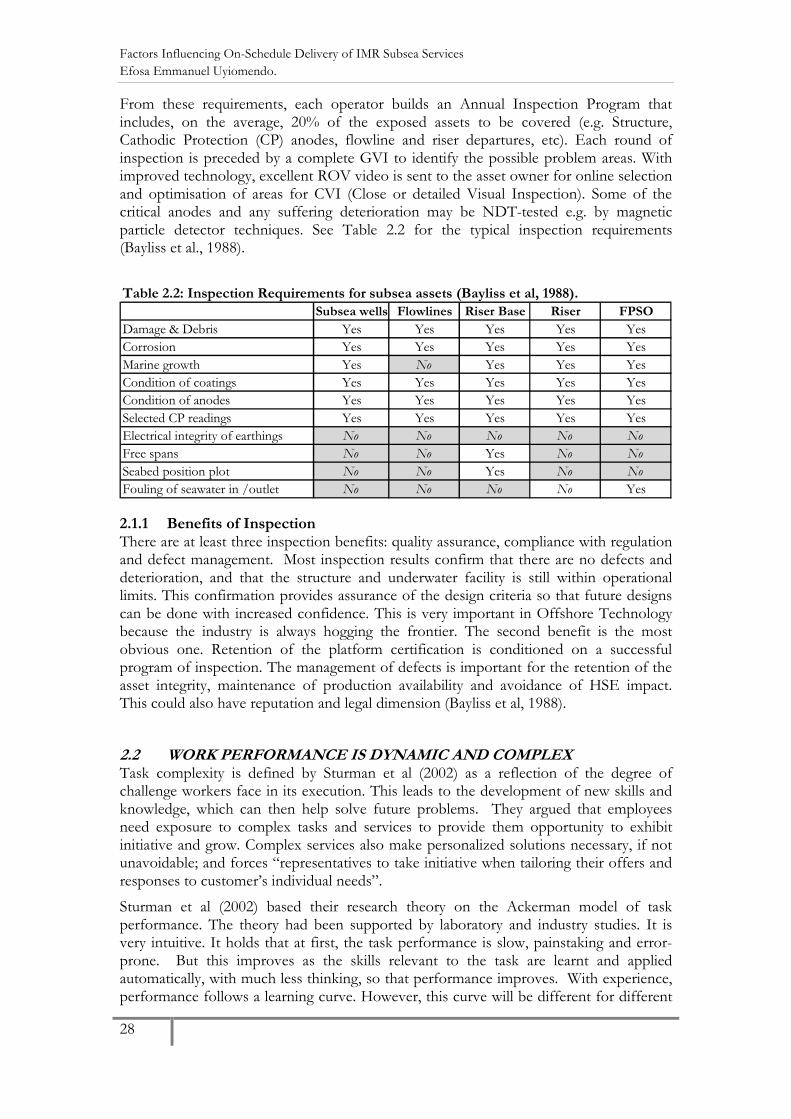
From these requirements, each operator builds an Annual Inspection Program that includes, on the average, 20% of the exposed assets to be covered (e.g. Structure, Cathodic Protection (CP) anodes, flowline and riser departures, etc). Each round of inspection is preceded by a complete GVI to identify the possible problem areas. With improved technology, excellent ROV video is sent to the asset owner for online selection and optimisation of areas for CVI (Close or detailed Visual Inspection). Some of the critical anodes and any suffering deterioration may be NDT-tested e.g. by magnetic particle detector techniques. See Table 2.2 for the typical inspection requirements (Bayliss et al., 1988).

Table 2.2: Inspection Requirements for subsea assets (Bayliss et al, 1988).

Subsea wells Flowlines Riser Base Riser FPSO

Damage & Debris Yes Yes Yes Yes YesCorrosion Yes Yes Yes Yes YesMarine growth Yes No Yes Yes YesCondition of coatings Yes Yes Yes Yes YesCondition of anodes Yes Yes Yes Yes YesSelected CP readings Yes Yes Yes Yes YesElectrical integrity of earthings No No No No No

Free spans No No Yes No No

Seabed position plot No No Yes No No

Fouling of seawater in /outlet No No No No Yes

2.1.1 Benefits of Inspection There are at least three inspection benefits: quality assurance, compliance with regulation and defect management. Most inspection results confirm that there are no defects and deterioration, and that the structure and underwater facility is still within operational limits. This confirmation provides assurance of the design criteria so that future designs can be done with increased confidence. This is very important in Offshore Technology because the industry is always hogging the frontier. The second benefit is the most obvious one. Retention of the platform certification is conditioned on a successful program of inspection. The management of defects is important for the retention of the asset integrity, maintenance of production availability and avoidance of HSE impact. This could also have reputation and legal dimension (Bayliss et al, 1988).

2.2 WORK PERFORMANCE IS DYNAMIC AND COMPLEX Task complexity is defined by Sturman et al (2002) as a reflection of the degree of challenge workers face in its execution. This leads to the development of new skills and knowledge, which can then help solve future problems. They argued that employees need exposure to complex tasks and services to provide them opportunity to exhibit initiative and grow. Complex services also make personalized solutions necessary, if not unavoidable; and forces “representatives to take initiative when tailoring their offers and responses to customer’s individual needs”.

Sturman et al (2002) based their research theory on the Ackerman model of task performance. The theory had been supported by laboratory and industry studies. It is very intuitive. It holds that at first, the task performance is slow, painstaking and error-prone. But this improves as the skills relevant to the task are learnt and applied automatically, with much less thinking, so that performance improves. With experience, performance follows a learning curve. However, this curve will be different for different


29

individuals as we have different “abilities, motivation and opportunities”. The dynamics in performance can be of two forms. They could arise from changes in the people executing the tasks or providing the services e.g. through training or motivation. This is known as the Changing Subjects Model. They could also result from changes in the “determinants of performance” i.e. Changing Tasks Model.

In this Masters Thesis, our focus is on the task-related factors that determine performance variability. This does not mean that motivation and knowledge are less important. We have taken the view that data on the task factors that might influence performance would be cheaper and easier to gather. The Project has an extensive record going back 9 years on such parameters as the job location, water depth, equipment performance, elements that influence task difficulty, procedures adopted, detailed job reports and so on. On the other hand, records of motivation and knowledge levels of staff are not that rigorously kept. Arguably, this could have been measured. It is true that the knowledge of crew would be important. The contract specifies a minimum experience, qualification and job category of the personnel that must be on the vessel (Offshore Manager, Senior Project Engineer and Project Engineer, etc), and these requirements are always complied with, sometimes even exceeded. Also the Client representatives are always on board the vessel. Then there are very capable specialists in the operation of the ROVs, Cranes and Module Handling Systems. Together, the operation crew of circa ten per shift have over 100 years of experience as well as industry based certification. This was the case over the period of the study i.e. 2006 to 2008.

Thus, it can be assumed that the only Subject Model variable of relevance would be the motivation level of the employees of the Project. However, as earlier observed, this is not recorded. Projects are usually highly resulted-oriented (Gardiner, 2005). The author has witnessed several sessions of focused and dedicated application of knowledge and expertise in a team based environment. We have assumed in this Masters Thesis that motivation was not an issue (i.e. held adequate and constant).

2.3 ORGANIZATIONAL AND JOB LEVEL COMPLEXITY Complexity can occur at all levels of on organisation and at their work processes. It can also be viewed at the level of jobs and tasks i.e. the difficulty involved in executing them.

2.3.1 Organizational complexity and high-technology firms Von Glinow and Mohrman (1990) proposed the following four intuitive identifiers for high technology firms:

• Employs large proportion of scientist, engineers and technologists. • High percentage of research and development spend (twice the industry average). • Emergence of new technology renders old technology obsolete. • Potential for extremely rapid growth.

People in these organisations are valued by their technical expertise which they must maintain up-to-date to remain relevant. Valuable expertise is derived from different disciplines and specialities. They are combined to solve complex, “ill-defined and elaborate” projects with “multiple puzzles” whose solutions must be mutually compatible in a workable system of tasks. In addition, the complex system of tasks and people exist in an environment that is constantly changing and therefore uncertain.

The foregoing is a sound description of the study Project. Each IMR job or “maintenance project” is usually loosely defined. The Project must integrate a range of


30

in-house and external expertise to deliver the IMR service to the Client specifications and within the capabilities of the IMR; using own & hired equipment, and executing these safely, efficiently and effectively.

2.3.2 Forms of job level complexity At the level of jobs and tasks, Complexity may be seen in terms of the difficulty of solving a problem – measured in time and in space i.e. memory requirements (Barringer, 2008). The approach adopted for the modelling of the associated complexity was inspired by literature such as these, own experience, reviews of previous job reports and interviews with Project Leaders.

Richardson et al (2004) investigated the relevance of seven task variables to assembly operation complexity. The variables were hypothesized through task analyses and then studied using statistical multivariable analysis. From these, they proposed a prediction model for assembly complexity. It took the form of a model of complexity or the level of difficulty based on (a) the number of components; (b) the symmetrical planes; (c) novel assemblies; (d) the number of fastenings; and (e) the number of component groups. Together, these five valid variables had an R of 0.76 and R2 of 0.56. This implies that 56% of the variations in the level of difficulty were explained by the modelled factors.

DNV-RP-H101 (2002) “Risk management in marine and subsea operations” lists seven assessment parameters, including:

• Marine operation method (novelty, feasibility, robustness, type, previous experience) • Personnel exposure (qualification, experience, required presence, shift arrangement) • Equipment used (margins robustness, condition maintenance, previous experience, suitability, experience with operators or contractors);

• Operational aspects (language barriers, season environment conditions, local marine traffic, shore proximity);

• Existing field infrastructure (surface and sub-surface); • Handled object (value, structural strength / robustness); • Overall project particulars (delay, replacement time / cost, repair possibilities, number of contractors’ interfaces, project development period).

The last parameter is an outcome in the context of this Master Thesis. The penultimate two relate to the physical infrastructure and can also be ignored. As discussed earlier, we decided to exclude personnel factors for pragmatic and practical data availability reasons. The remaining three parameters (marine, equipment and operational aspects) have important issues that were corroborated during interviews with the Project. These include novelty of the job, equipment condition, experience with the tool, and environmental conditions (or seastate which is often measured by significant wave height).

The difficulty with physical complexity is that there are several possible formulations. Edmonds collated up to 40 different such formulations. Some of these are shown on Table 2.3. Many of them have wide applicability and can be extended to IMR subsea services.


31

Some Formulations of Complexity (Edmonds B., 1999)Formulation Credit Definition Strengths & Limits

1 Abstract Computational

Complexity

Blum, M. A.,1967 Set of decidable computation functions in time and

space.

Influential. Too broad, sub functions

maybe more complex.

2 Algorithmic Information

Complexity

Solomonoff R.J., 1964;

Kolmogorov A.N., 1965;

Chaitin G.J., 1966

Length of shortest program to produce in a Turing

machine. Ordering reduces complexity

Influential. Skewed towards

Information theory

3 Arithmetic Complexity Girard, J.Y., 1987 Min. no of arithmetic operations required to complete a

task

Practical & encourages efficiency.

4 Cognitive Complexity Kelly, G.A., 1955 Dimensions of inferred mental mode in discuss of

personal constructions

1D cognitive Simple, 2D more

complex.

5 Connectivity various; e.g. Winograd

S., 1963.

Level of interconnections between system components. Reliability, chemical rxns,

competition networks, ecosystems

etc.6 Cyclomatic Number various: e.g. Temperly

H.N.V, 1981; Hops JM et

al 1995.

No. of independent loops in a graph. n(G) = m - n + p,

where m = # arcs, n # vertices, p # disjoint partitions the

graph divides into

Captures interconnectedness. Army

heirachy reduces complexity.

Committee max. comms channels

allows unpredictable to happen.

7 Descriptive/

Interpretative

Loofgen, L., 1974. Difficulty of encoding realisation (building blocks, e.g.

DNA) into a descriptive whole and decoding back.

Uses Kolmogorov for description &

Logical depth for interpretation.

8 Dimension Attractor Baker, G.L., 1990. The extent a process can be modeled, its attractor in

state space, forms a system of converging dimensions

Fractal with chaotic processes.

9 Dimensions Lugosi G., Zeger K., 1996 The no. of irreducible or unique dimensions in a system

guides its complexity

Applied to concept learning

10 Ease of Decomposition various: e.g. Conant

R.C., 1972

Ease of decomposing the system into it sub-components Extensively applied.

11 Economic Complexity various, e.g. Arthur B.,

1994

Where some or economics simplifiying assumptions do

not hold, complexity results.

Agent Theory is one example.

12 Entropy various e.g. Cornachio,

J.V., 1977

The more disorder (entropy) a system has the more

description information required and more complexity

Essentially probabilistic

13 Goodman's Complexity Goodman, N., 1966. Complexity of a system is the sum of the complexity of its

predicates

14 Horn Complexity Aanderaa S.O. & Boorger

E., 1979.

Min. length of a Horn formula that defines a function. Related to network complexity

15 Inequivalent Models Mikulecky D.C. 1995 Presence of multiple inequivalent models describing the

same system.

16 Info. Gain in Heirarchical

Approx. & Scaling

Grassberger, P., 1989. A system is complex if it reveals different laws

(interactions) at different resolution levels.

Captures information increase with

increasing scale.

17 Information Klir, G.J. 1984 Amount information a system encodes or is required to

describe it.

Deterministicall equiv to AIC and

probabilistically eqiv. to Entropy

18 Irreducibility Nelson,R.J., 1976. That which is irreducible. like Decomposition

19 Logical Depth Bennett, C.H., 1988. Run time to generate object by incompressible program.

Random & simple programs have least depths.

Long computation or slow to

simulate dynamic process are deep

logically.20 Organised and

Disorganised Complexity

Weaver, W. 1948. Organised compl. occurs when a limited set of factors

affect the whole. Disorganised complexity occurs with

many ind. variables

Disorganised examples is accident

statistics, organised include

economic flucntuations

21 Size various: Carneilo, R.L. No. of parts increases potential for complexity Necessary but not sufficient

22 Symbols Jaskowski, S. 1948 No. of sysmbols is a guide to complexity. Necessary but not sufficient

23 Variables Diamond A.H. &

Mckinsey J.C., 1947

The no. of variables and its structure affects complexity. Necessary but not sufficient

24 Variety various: Bak P. &

Paczuski M., 1995

Likely to exhibit greater variety in behaviour Easily counted (types, sudden

changes etc)

For instance, the job of providing IMR service has a high degree of abstraction although the ROV-held cameras help to provide some context. Also, there are several dimensions to it, including marine operations, structure deployment analyses, material science, weather and hydrodynamics, maintenance engineering, etc. Jobs come in different levels of difficulty and thus require different levels of procedure steps to analyse and describe. The task plans of the most difficult jobs have several elaborate pictures to assist their visualisation, and others have no pictures whatsoever (there are no animations). This is akin to symbol formulation of complexity. In addition, the most complex jobs are broken into a series of standardised sub-tasks to increase their ordering and thus reduce complexity.

According to Goodman's formulation of complexity, a system’s complexity is related to the sum of the complexity of its parts. We know that the hydrodynamic response of irregularly shaped objects in water, The North Sea weather and ROV flight pattern (to


32

name only three) all require multiple variables for their description. Thus, each of these is potentially complex in theory. In reality, they are very much so. Each is a specialist discipline on its own. As IMR operations include or involve them, it can be inferred from Goodman's formulation of complexity that IMR services are complex.

Predicting the performance of such a complex operation will require multiple variables. One of the most frustrating properties of complex systems is that they are difficult to decompose (Edmonds, 1999). It could take a dozen variables to describe weather alone. For simplicity and convenience, the industry adopts significant wave height and wave length as key operability measures. Richardson’s works on task complexity is consistent with this simplification. We can not measure everything and remain efficient. In any case, the redundancy in the range of possible measures encourages us to limit the variables as much as possible.

Other measures considered for representing complexity include: (a) number of pictures in the procedure; (b) number of procedure steps; and (c) number of hold-points. The last measure is so important that sometimes independent witnessing is required (DNV, June 2004). Hold-points are “points in the procedure beyond which operation must not progress unless and until the authority is given by a specified person or organisation”. It is less common (or evident) in valve operations, and more common in module handling (MH) and light construction (LC) job types. In addition, this could be a good measure because it captures the number of intermediate outcomes that could influence how the job might progress, an indication of dis-organised complexity.

There tends to be more pictures in the more complex jobs. However, the number of pictures can increase because equipment is hired in, and not necessarily because the job is more difficult. Some job steps that are executed by OEM (e.g. module running tool operation) are not clearly described in the procedures. The number of procedure steps would have been problematic for this reason.

2.3.3 Uncertainty in jobs Through interviews and reviews of job reports, it became clear that, in addition complexity, another measurable reason why a job might be delayed is its inherent uncertainty. Whereas complexity relates to the difficulty or challenge the job requires, the uncertainty refers to our inability to completely specify a subsea intervention activity beforehand. This is not always a bad thing. Sometimes a job being executed correctly and on schedule is interrupted on the request of the Client in order to attend to a higher priority job. On returning to the original job to complete the remaining tasks, often the Project found that the level of efficiency achieved before the interruption was not immediately attained. Also, certain set-up and placement tasks for ROV and tooling have to be repeated. In essence, extra time would be required. We have decided to call this type of uncertainty Phasing. It is similar to setup losses that the Overall Equipment Effectives (OEE) measures seek to minimize in order to increase equipment availability (Liyanage, 2007, Sharma et al 2002+). Phasing is assessed from the completed job reports

Another uncertainty measure is Scope Change. Changes in job scope can occur on occasions when the some of the assumptions held about the job during its planning phase are found to be incomplete or incorrect on site. Access to the critical modules may be restricted and needs to be improved or created. The tool may not match even if the correct type had been selected. It would need to be modified quickly and effectively. All of these would take time which could lead to slippages. Scope changes are also assessed from completed job reports.


33

Finally, a third aspect of uncertainty is the Management of Change (MOC). This is the controlled process of adjusting the prescribed procedure for executing a job. The need for this could arise if the Senior Project Engineer finds that this original procedure can not be adopted due to miss-match, access, unavailability of tools and equipment, or for some other reason. The MOC is documented according to the Project Guidelines. It is suitably approved and included in the Offshore Report. The complete MOC records are kept on the vessel so it was more efficient to access this information directly.

The distinction between MOC and Scope Change is subtle. Scope Change is normally requested by the Client, whereas MOC is a control process implemented by Project over a change considered risky or significant. The most common form of SC is when an agreed and ongoing sequence of work is interrupted and a new stream of activities executed before the original stream is resumed at the original point of interruption. If all these activities are low risk or generic (e.g. inspection, anchor assistance and valve operation) a well developed task plan and HIRA could be enough to control the change process. Sometimes, the Client requires not only the addition of new activities, but also a complete change in the sequence of existing activities. MOC process is always done these types of changes, as a control. The same event could lead to both MOC and Scope Change. Some only cause a Scope Change.

2.4 SERVICE INNOVATION IN HIGH TECHNOLOGY FIRMS As noted in section 2.3.1, IMR processes are inherently innovative because of the unique service contents delivered in each job. Now, service innovation is generally more demanding than product innovation. The former also involves changes in the delivery process, interface, relationships and performance (Gerbauer et al, 2008). The history of innovation models (Table 2.4) reflects these increasing linkages and the increasingly more complex contexts in which service innovation must occur. An example of such a collaborative environment is depicted in Figure 2.1. It features a production facility which is the focus and beneficiary of applied resources from the operator and a range of service providers (Panesar & Markeset, 2007). This is not unlike what happens in IMR service delivery. The degree of innovativeness may be described as (a) Radical, i.e. new to the world; (b) “Me Too”; or (c) Incremental. Companies that have formal service innovation processes are more likely to have successful innovations (Oke, 2007).

Table 2.4: Innovation Models (summarised from Panesar and Markeset, 2008)

Year Generation Theme Strengths

1950s First Linear Sequential model Technology driven

1960s Second Market Pull model Market driven

1970s? Third Coupling model Market, technology & scientic progress feedbacks.

1980s Fourth Integrative model Cross-functional integration across disciplines & companies

1990s Fifth Strategic linkages Strategic links with suppliers/ Customers, employees and speed


34

Fig 2.1: Service Collaboration for Production Facility

(taken from Kumar and Markeset, 2007)

Authors agree that the initiation or idea generation stage is the first-step of all innovations (Gebuar et al, 2008; Panesar and Markeset, 2007; Oke, 2007). This proposes a method to improve the customer offering or the processes for delivering them. It can be internally or externally driven, or even from a special R&D department. Each of these ideas is then evaluated against the organisation’s decision making factors, and the best ones are selected for implementation. Decision making factors include: (a) return on investments, (b) availability of raw materials, (c) innovation costs, risk of failure (d) availability of external competence (Panesar & Markeset, 2007).

Even when the work context (Figure 2.1) emphasises resource flow, there are technology (new technical requirements), market (customer or facility needs) and integrative pulls in the process which can all encourage innovation. The cross-functional teams provide ongoing input and feedback. These “pulls” was observed in IMR study Project. Each specific requirement is discussed widely by experts until the most optimal solutions are short-listed. There are several levels of interaction (management, project manager level, technical manager, Project Engineers and Offshore between Project and Client reps). Formal multi-discipline meetings are also held to review the solutions options, risks and schedules.

In another paper, Parnesar and Markeset (2007) propose an alternate taxonomy including operational needs, return on investment, market position, contractual relationships, service gaps, service relationships and organizational environment. These are very relevant to a competitive situation. Perceived gaps in product market position can be a strong incentive to invest in innovation, irrespective of the risks or investment required. For instance, in 2007 the IMR Project vessel was taken to dry dock in the middle of the contract. The resulting upgrade raised the vessel’s weather tolerability for ROV operations to 5m (among other things). This had become the Industry standard from the new contracts awarded in that year. Thus this was a “me-too” investment in innovation (higher ROV operability) necessary to remain competitive in their target market.

In most cases however, each job aims at delivering pre-agreed results on an existing installation. If innovative solutions are proposed they are reviewed and integrated. Right up to job execution, the Project has procedures for considering and approving changes to task plans (e.g. Management of Change). Sometimes, the Project is specifically required to develop a feasible solution for an innovative or a very new job.


35

2.4.1 Factors influencing service innovation Panesar and Markeset (2007) validated five key drivers of innovation in the Oil & Gas Industry of Norway. Others include (a) customer initiatives and feedback; (b) new or improved technology; (c) employee initiatives & feedback; (d) Government regulation; and (e) lateral learning from similar services.

Their surveys and analyses show that market needs and customer feedback are the most important drivers of innovation. Service providers such as Aker Solutions, Acergy and Seadrill collaborate with Operators such as StatoilHydro, BP and ConocoPhillips to develop new solutions, which can improve the overall effectiveness and efficiency of their business processes. The other factors are no less important. Firstly, they tend to drive market needs & Client feedback. Secondly, regulation can be very prescriptive (e.g. CO2 sequestering).

In another study of Contractual Relationships’ influence on innovation, the same authors concluded that “the development of appropriate contracts is essential to creating an environment for service innovations and continuous improvements”. Gerbauer et al (2008) and Oke (2007) found that healthy (i.e. creative and open) internal organisations foster more fruitful innovations. These can be demonstrated by a clear strategy and the level of resource provided.

IMR jobs are inherently innovative. New underwater barriers are constantly being broken. New tools and procedures are frequently introduced. Some jobs are generic (see Figure 2.2) i.e. recurring quite frequently, but most jobs have several sets of an appropriately modified “solution” that serves the current requirement. Solutions are defined as: “A defined group of components (equipment, tools, procedures and services) which when integrated together will resolve a customer’s complex problem” (adapted from Shepherd & Ahmed, 2000).

2.5 MAINTENANCE PROJECT PERFORMANCE MEASUREMENT Each IMR job is organised as a maintenance project (for a discussion see Coetzee, 1997). It has a unique goal e.g. “Replace SCM at Troll BCD”, it is temporary and resources are assigned to it for these specific tasks (Gardiner, 2005). Depending on the job type, the Project may hire in other resources from third parties at agreed rates.

Thus, 3 groups of resources are mobilised for the project execution: Project (the provider of Ship), Client (owner of facility) and Hired- in Resources (third parties, including OEMs). The Client maintains a rolling schedule of the jobs. These are updated each week (duration, sequence of execution, and, occasionally, objectives). As the Ship and each of the resources are charged per unit time, the planned and actual schedule drives budgeted cost and actual cost performance, respectively.

In addition, a large proportion of these jobs have hydrocarbon tied to them. Thus, the speed at which the services are delivered also influences the Client’s revenue. This is an incentive to progress jobs quickly through the planning phase to Offshore for execution (see IMR Work Process Figure 2.2).

This is almost always possible for routine jobs like Valve Operations and Condition Monitoring. To a lesser degree, jobs with standardised solutions like Module Handling can also be planned fairly quickly. However, some jobs are so unique and / or complex

Fig 2.2: IMR Work Process


36

that sufficient time is required for the development of unique solutions for them. For instance, the planning phase of tie-in and light Construction projects could take months, as unique tools and solutions need to be developed. They are also more likely to require more vessel time for execution.

2.5.1 IMR contract forms and structure There are two common forms of major contracts in the Norwegian Industry: Maintenance and Modifications (M&M) and Performance Based Operation (PBO). M&M contracts pay a fixed sum for a fixed scope of work that is defined by the service receiver. In PBO contracts, some portions of the payments depend on the service performance. The scope of work is flexible: the possible options, changes and variations are specified by the Client. Actual payments are linked to the quantity and quality of service delivered (Kumar & Markeset, 2007). Thus, there is a profit incentive for the service provider to deliver high quality services from the start.

IMR contract is a mixture of both of these types. There is a fixed day rate for the vessel and for each of the items on board. However, the actual delivery schedule is not fixed. If the job takes a little longer than planned due to increased difficulty or “scope creep,” the extra scope is executed and the Project is compensated. If there are weather delays the Project receives a lower day rate. Lost time due to equipment breakdown is charged at progressively lower rates, depending on degree of operability. Thus, there are sufficient incentives for the Project to specify very high reliability for the equipment used.

However, the incentive for efficiency is less clear-cut. There is at least one Client Rep aboard the vessel at all times. The Client manages the schedule and determines its priorities. The Client also approves and supervises the job procedure. There are several hold-points where the Client checks and approves progress. One can thus conclude that the Client is partly responsible for efficiency in the short-term. In the longer term, the Client is in the position to review the numbers of jobs executed with her annual budget, and obtain an idea of the overall efficiency of service delivery. It is likely that the Client would embark on this sort of review during contracts renewals and extensions. Thus efficiency is important in the longer term.

Kumar and Markeset (2007) identify five types of maintenance contracts as shown on Table 2.5. IMR services for subsea assets can be described as Type 3 i.e. Product + Total Service. The Operators buys in all the routine and non-routine maintenance (including repairs) that is required to retain the reliability and availability of the subsea assets.

Table 2.5: Types of maintenance contracts (Adapted from Kumar, R., Markeset, T. and Kumar, U. 2004)

Types Owner Process Perf Routine

Maintenance

Specialised

Maintenance

Spares /

Tools

Remarks

Product

1 Traditional Opco Opco Opco OEM OEM

2 Product +

maintenance bundle

Opco Opco Opco or OEM OEM OEM

3 Product + total

service

Opco Opco & OEM OEM OEM OEM Availability &

reliability onlyProduct

Solutions

4 Solutions selling Opco Opco & OEM OEM OEM OEM Sells performance

and function

5 Total care OEM OEM OEM OEM OEM Helps Opco realise

visionSolutions


37

2.5.2 Measures for project performance The reasons for performance measurement and management are to “check position”, “communicate position”, “confirm priorities” and “compel progress” (Amarantunga, 2002). In addition to the scale and scope economies that defined the industrial age, companies are developing intangible assets. These include developing customer relationship and knowledge workers, the introduction of innovative products, and deployment of IT. To enhance capture over the longer-term and harder-to-measure competitive measures, models such as (a) Balanced Scorecard (BSC), (b) EFQM and (c) Scandia Navigator have evolved. Each model measures results and its enablers, over the long-term and against the company strategy. They all recommend the development of people and relationships to drive innovation. However, only EFQM is inherently scaleable (applicable to businesses of all sizes). Just like BSC perspectives, Scandia’s mission statement is difficult to define for business groups or away from the very top of the firm. EFQM and Scandia have much better coverage over intellectual capital and stakeholders than BSC (Liyanage, 2008; Marr and Adams, 2007; Neely et al, 2000; Uyiomendo, 2008 unpublished).

Thus, EFQM kind of model could be used for the performance management of IMR projects. This is a nine criteria model that was jointly developed by European industry in 1988. The first five criteria are enabling i.e. describing how organisations should undertake her activities; the last four criteria describe the actual results. Excellence in performance, customers, people and society are achieved through leadership driving policy and strategy that is delivered through people, partnerships and resources / processes. It is the only model that requires a self-assessment.

However, experts consider this scaleable model even too top-level and extensive for project performance management (it is also considered too extensive for this Masters Thesis). Projects are temporary, the products are different each time and the concept of customer is dispersed and changing (e.g. see Gardiner, 2005). To choose an appropriate measure of project performance, the author considered both the literature and the data availability. A very good measure may be impractical because the retrospective data may not allow its computation (Waal et al, 2007). After a review of literature and practice (DOE, USA), the committee setup by DOE proposed a comprehensive list shown in Figure 2.4.

Figure 2.4: Project Management Measures (USA DOE National Reasearch Council

Project-Level

Output/Outcome

Program- and Department-Level

Input/Process Measure

Program- and Department-Level

Output/Outcome Measure

1 Cost growth Project director staffing. Assess project perf. (Green / Yellow/

Red).

2 Schedule growth Project support staffing. Time projects remain yellow or red.

3 Phase cost factors Senior Management involvement. Mission effectiveness.

4 Phase schedule

factors

Commitment to project Green 0.90 to 1.15

5 Preliminary

engineering and

Identification and use of lessons

learned.

Yellow 0.85- 0.90 or 1.15 - 1.25

6 Cost variance Independent reviews & impl of

actions.

Red <0.85 or >1.25

7 Cost performance Number and dollar value of

8 Schedule variance Project performance wrt project

size & contract type.

9 Schedule Use of good project management

10 Safety performance

The singular most appropriate measure is the schedule variance. A measure for this is Schedule Performance Index (SPI) (budgeted cost of work performed/actual cost of


38

work performed). As shown, the Research Council proposed a double-sided grading system for Green (90 - 115%), Yellow (85 – 90% or 115 – 125%) and Red (<85% or >125%). Simplified and applied to the case of IMR, SPI is equivalent to the planned duration/actual duration. This is so because each item on board the vessel has a fixed hourly rate once mobilised and operational.

David Malloy observed that SPI is a lagging measure that is often weeks and months old when computed. In addition, it is likely to be optimistic (as it may not capture reworks and errors). It is also difficult to use as a management lever as it reflects “only known past, problems”. This is a very harsh criticism. In the case of IMR the execution duration includes rework and error correction time, so the calculated SPI is representative. Similar jobs are repeated at different sites. Thus, learning points can be carried to subsequent jobs in terms of adjustments to schedules, tools or procedures. If a pattern exists in a set of projects reviewed, it may point to systematic issues that could be resolved proactively for subsequent campaigns.

Gardiner P.D. (2005) demonstrates how SPI can be used for management reviews. The context was projects of several months and years of duration. The projects undertaken by IMR have durations of days and weeks. In this case, the learning points from reviews would be more useful for future projects in the short-term (in addition to management reviews). This is the case in our retrospective study. Given the data available, this measure is arguably the most appropriate.

Thus, SPI will be used as the dependent variable in our investigation. The aim of this research then reduces to determining the independent variables that influence SPI.

2.6 ENVIRONMENTAL FACTORS The environmental factors which can influence operations in The North Sea include waves, current, wind (speed and direction), ice and snow fall, air temperature, sea temperature (Gudmestand, 2008; Norsok N-003, 2007). Given the common operational areas of the vessel, wave height and wave period are the most important measures of operability (Hovland, 2007). See also section 1.3. When the weather is not favourable the operation “waits on weather”. This contributes to delays.

Another environmental element that will be modelled is water depth. The Project IMR vessel was commonly deployed to intervene in subsea production systems installed at between 70m to 1100m. The shallower the operating water depth, the shorter the time that may be required. Although less obvious, the lesser, too, would be the potential for delays because of the reduced running in period.

2.7 MAPPING OF INFLUENCE FACTORS AND DEVELOPMENT OF HYPOTHESES

Based on the foregoing literature survey, a number of hypotheses are hereunder developed for testing. These relate to water depth, weather, complexity and job uncertainty. They are enumerated below.

2.7.1 Influence of water depth on operations A number of tools are used in sequence during IMR operations. Many of these are carried to sea bottom on the tool basket. However, a significant proportion of the tools require tripping to the surface for selection, installation and configuration. These include complex tools, tools requiring calibration to ROV and valves before use, and heavy tools.


39

For these cases, setup and tool changes would take more time in deeper operating conditions are. In addition, the effects of water pressure and the associated resistance increase with water depth. Longer ROV umbilical and winch crane wires are required for deeper waters, and the risks of entanglement increases with depth (requires slower ROV sailing or “flying” speed). In addition, direction of current varies as depth increases.

Wave interaction with sea bottom reduces visibility, which could potentially slow operations down. The effect of this is strong down to half the wave length. Strong water currents could also constrain operations by causing guide wire “blow” (although this also depends on the location). Another important effect of working in deeper waters relates to breakdowns (discussed below). Repairs of equipment in deep waters would require more time just to retrieve it to the surface.

One could argue that IMR equipment has been designed for 1500m, and so should not be constrained at all operations within these depths. In addition, the use of techniques such “Constant Tension” should limit GW blow. The “design” argument is also a possible counter for visibility (ROVs have at least six very powerful underwater lights) and water pressure (there are six or seven power thrusters for movement in all directions). It is true that specification of high reliability equipment avoids breakdowns. But equipment breakdowns do occur, and when they do, there is no short-cut method to retrieve them to the surface for repairs.

H1: Does SPI increase with an increase in water depth?

2.7.2 Influence of weather disruption Some IMR operations are highly sensitive to weather (weather limitation of circa 3m Hs). In this group includes Module Handling and Light Intervention. Valve Operations and Condition Monitoring can be executed at Hs of circa 5m. The Project has access to online weather forecasts which are reliable. However, these are not infallible. Once an operation is planned, the least weather tolerant item can stall it. The project copes with this by breaking the job into portions with different weather tolerability. The sub-tasks could then be phased but their sequence must be in an acceptable order. Different jobs (VO, CMM and MH etc) with differing tolerability would allow flexibility to select jobs more appropriate to the weather forecast, provided there is no fixed succession relationships prescribed by the Client.

Even within the weather tolerability limit, equipment lifts and transfers; personnel movement, motivation and sharpness could all dip in a terrible weather. The Offshore team is empowered to cease operations when it is considered unsafe to continue. The Project treasures her very impressive safety performance.

H2: Does SPI increase as weather becomes less favourable?

2.7.3 Influence of equipment availability Besides weather, another possible operational disruption is equipment breakdown. The vessel runs a very tight operation and with very little sparing. For now, the vessel and crane can be assumed to have 100% reliability. Nothing works without the vessel and the more complex operations require the crane. In this Thesis, reliability discussions are centred on the ROVs. The Project ROV reliability reports show 97% average performance for both hired and owned ROVs. Now Condition Monitoring and Valve Operations can be done with a single ROV (with some stretch, either ROV if the required torque is low). Both ROVs are required simultaneously for MH and LC jobs. So a failure in any one would delay these more complex jobs. Thus CM and VO could be disrupted or interrupted by simultaneous failures on the two ROVs i.e. (1 – 0.032) =


40

99.91%. MH and LC requires at least one failure i.e. both must be working = 0.972=94.09% (See Aven, 1991)

The running tools and MHS have even more specific roles. Spares and competence for repairs are retained on the vessel but down time causes loss of revenue for both Client and Project. Potentially, each breakdown could cause delays whose duration depends on how quickly repairs can be carried out. If we assume spares and competence are always available, this is a function of working conditions i.e. weather, as the vessel is a 24hour work place. A breakdown during a precious weather window could cause a longer delay i.e. the “butterfly effect”.

Hired-in equipment deserves a special mention. These are used for peak shaving and the more specialised jobs. Hired-in ROV reliability performance and expectation is high (4.5%) but not quite as high at the 2-3% set for Project owned ROVs. At least in one case, work was delayed after a failure on a hired-in ROV because the spare could only be located in another country. As a significant proportion of equipment is hired-in this risk is considerable. Overall, the breakdown records for ROVs are very good.

A less obvious issue relates to MH jobs executed with some degree of urgency. These require a ready OEM running tool plus a new module for replacement. Modular replacement policy can limit deferment from the well through rapid response. The readiness of such Client Provided Items (CPI) can delay "rapid response" jobs.

H3: Does SPI increase with increasing equipment unavailability?

2.7.4 Influence of job complexity Complexity relates to degree of difficulty (in time or space) required to do things. The more complex an activity is, the higher the potential for errors, rework and hence delays in specified time (Barringer, 2008). As discussed in section 2.3.2, we can recognise complex jobs from their lengthy procedures, elaborate pictures, new or exotic tools, very heavy lifts and prescribed vessel interactions, etc. The more novel a tool or procedure is, the longer the time that is required to learn and perfect it. The less perfectly an operation is understood, the more prone it would be to surprises and errors. Thus, we expect usage of novel tools to potentially lead to more delays, when compared to generic tools. In practice, such new tools are subjected to FAT (factory acceptance test) and trial runs at the workshops. These simulate operational conditions for the Project Engineers.

In the same vein, the most difficult lifts are potentially slower to execute and prone to more disruptions. It is not unusual for these awkward and heavy lifts to have deployment analyses specifying very narrow windows (in terms of wave height, water currents and wind speeds) for the operation. These require precision, a lucky gift from nature and lots of patience. They could also create potential for delays.

A less obvious dimension for complexity is the number of contractor interfaces. This often correlates with the different types of OEM tools on board the vessel. A clear communication protocol is laid down for managing these interfaces. In addition, the procedure for the most complex jobs has “hold-points” prescribed to confirm and record conditions before the job continues.

H4: Does SPI increase with an increase in job complexity?

2.7.5 Influence of job uncertainty Each job starts and closes with a site survey. Even then, site assumptions can be quite different from reality on arrival. This could be due to, say, the activities of third parties,


41

incorrect labelling or an active sea bed. Before the job can proceed, the procedure would have to be amended in some way. This is a different kind of disruption.

Even when all is well, the Client priorities could change. The work scope can change with new information. Extra time would then be required to propose, analyse and approve changes. The job procedures usually specify precautionary tests on guide wires and protective covers (and other exposed items) to reveal any weakness(s) under safer conditions. Should any be revealed, they must be corrected before work can progress. It is difficult to allow time for these on the schedule because one does not know if any or how much would be required.

Some procedures do have contingency built in. These are clear steps that maybe required as a course of action should something else occur. These alternative steps that could lengthen or shorten the average duration. The scheduled time would be based on the base procedure (and not the contingency).

H5: Does SPI increase with increase in job uncertainty?

2.7.6 Influence of complexity mix Here we want to investigate if the availability of jobs with different levels of weather sensitivity would facilitate optimisation of vessel time, reduction of disruption and improvement of efficiency. In theory, this should be the case as between 3m and 5m Hs,, Valve Operations and Condition Monitoring type jobs can be executed. Such simple, short duration jobs are easier to fit into a narrow weather window. However, the tool requirements for these jobs are different and sourced differently. Once a running tool is picked from an OEM it has to be paid for. And these running tools are very job and template specific. Thus vessel time might be saved, but OEM equipment & personnel time might still be incurred. In addition, wells with production shutdown could loose huge revenues. The lack of standardisation in modules and running tools exacerbates this.

The overall schedule does show a mixed flow of job types. It is unclear the extent that this is accidental and the extent that it is intended. What is clear is that as the Client owns the schedule, the Project has only an advisory influence.

H6: Does SPI depend on job complexity mix?

2.7.7 Is the Project getting more innovative This hypothesis must be considered in relative terms over time. As noted earlier, innovativeness can be radical, “me-too” or incremental. In this case, we are more interested in whether there is more innovation now than in the past. The subsea industry has witnessed substantial technology-based innovation. The industry is always pushing depth & completion boundaries for subsea installations, especially in the North Sea. In IMR service in particular, there is a general drive for the improved procedures and safe practices, which can extends weight, weather and equipment limits. Given the above, is the Project in tune with these developments? Could it be ahead of the game?

We know that that since 2007 it has focused on maintenance and repair job types. Each of these is potentially complex and provides an opportunity to innovate. The Project has the critical mass of engineering skills and total knowledge to innovate across the technical interfaces required for IMR. The meetings and team style encourage this. Project leadership recognise that, with increasing competition, both innovation and efficiency may be required to retain market share.


42

On the other hand, a ten year contract with fixed hourly terms provides very little incentive for innovation in an inflationary market. The options in the contract did encourage some vessel upgrade but they were of the “me-too” type. The cautious culture of preferring only tried and tested solutions with minimal extensions also serves to control the pace of innovations. The wide range of mutually compatible tools, methods and equipment could not have been very helpful.

H7: Is Project getting more Innovative?

2.7.8 Is the Project getting more efficient? Cost is never the only issue but it is hardly a non-issue. The Client budget has ceilings so if jobs are not efficient, the number of jobs executed falls off, and revenue from oil receipts could drop (depending on the extent to which oil-sensitive jobs can be prioritised). The culture of applying learning from previous jobs aids innovation as well as efficiency. The Project Engineers and Client Engineers will review the procedures for effectiveness first but also for efficiency. This continues offshore. It is not unlikely that top level reviews are conducted between Project and Client to see if there are opportunities for efficiency gains. The fact that the Client owns the schedule means changes to it could potentially be less responsive than desired in certain situations. It can be argued that as the project executes deeper water projects (e.g. Barents Sea) efficiency could fall off with increasing water depth. By a similar argument, older facilities, more complex tooling and field-life extensions could potentially impact on efficiency.

H8: Is the Project getting more efficient?


43

3. MODELLING AND PREDICTION

In this chapter, we will review the tools and techniques that will be used for modelling and analyses. Included are multi-variable regression and Bayesian inference.

3.1 MULTI-VARIABLE REGRESSION ANALYSES Events of all types (medical, political, social, dynamic etc) have multiple causes or risk factors. Multivariable Analysis (MVA) is a statistical tool for determining the relative contributions of different causes to a single event or outcome. For example, a MVA on disease prognosis might consider factors such as the pathogen(s), strain virulence, exposure route, exposure intensity and immune response. For example, risk factors associated with premature mortality includes notably smoking, a sedentary lifestyle, obesity, elevated cholesterol, and hypertension (Katz, 2006).

Such a relationship could be described as linear combination of factors in the form

ii XbXbXbXbXbaY ++++++= .......44332211 3.1

Y is the value of the dependent variable, what is being predicted or explained. The constant "a" is the intercept, and bi are the slope (beta coefficients) for Xi, etc.

In longitudinal data analysis, the important aspects of several subjects are measured repeatedly over a period of time. In cross-sectional studies a single aspect is tracked for a given subject. The former is more powerful because it allows changes with time and differences across people to be separated. It can detect changes within the same subject or individual over time (known as ageing effects), and distinguish these from baseline differences across the subjects (Diggle et al, 1996).

Taris (2000) distinguished between mere association (termed co-variation) and causal links between variables. Relationships of associations can only support conclusions of the type “if X is the case, Y is usually the case as well” and “members of group a have on average more of the property X than members of group B”. Correlation coefficient (ordinal) or chi/square (qualitative) value would indicate the degree of association (Taris, 2000). Statistics can only prove association and not cause (Katz, 2006). Causal relationships allow one to reach conclusions such as “Y is affected by X” which is more powerful for the understanding of the phenomenon and prediction of future changes. Three criteria need to be satisfied for causality to be assumed:

a) Co-variation: there must be statistically significant association between the two variables of interest (co-variation);

b) Non-spuriousness: the association must not be due to effect of other variables i.e. by ruling out alternative explanations and

c) Temporal order: the “causal” variable must precede the “effect” variable. (Taris, 2000).

3.1.1 Regression analysis assumptions The assumptions of linear regression analysis include the following (Brace et al, 2006; Brown, 2004; Miles, 2001):

• The sample must be representative of the population. • The independent variables are error-free.


44

• The independent variables must be linearly independent, i.e. it must not be possible to express any independent variable as a linear combination of the others.

• The errors are uncorrelated, and the variance of the error is constant across observations.

Our aim is to conduct a multivariable analysis on a set of existing data about IMR jobs executed between 2006 and 2008. For each job category, we have between 30 and 60 jobs (206 in total). Only the set of jobs for which we have complete data was included. All these jobs would be analysed to determine the regression coefficients.

We assume that the jobs that were excluded (i.e. for which there is no detailed Offshore Report) are random i.e. these cut across job types. In reality most of them are annual inspections. In any case, these jobs are executed by the same vessel using what is effectively a near constant “tool box”. The crew may change but the crew competence is constantly at, or above, the level required for the job undertaken. We assume that each job is sufficiently planned and the organizational knowledge available for the Project is brought to bear before and during execution. In effect, we hold the organisational complexity constant and assume that schedule variance depends only on task complexity. This is a huge assumption.

Taris (2000) explored the range of possible errors possible in retrospective study. Included are memory errors and reporting errors. By providing appropriate cues in the assessment templates, memory errors can be minimised. The extremely detailed reporting system available also aids the error-free recall of the details of the job execution. Jobs with insufficient detail were excluded from the analyses for this reason. Reporting errors are generic to all forms of research. The use of several levels of reviews should limit these to a negligible level.

3.1.2 Reviewing multivariable analyses results Three key results from MVA that are often used to check the quality of the MVA output are as follows (Miles, 2001; Brown, 2004).

• R2 value of the entire analyses: this indicates the proportion of the variations of the independent variable explained by variations in the dependent variable. This value can vary between 0 and 1. The adjusted R2 value relates this to the number of variable used.

• Standard error of the estimate (SEE) is a representation of the standard deviation of dependent values around the regression line.

• P-value of the coefficients: these have to be below 0.05. Any that is not is regarded as not significant.

• Standardised coefficients are used to rank the relative influence of the factors.

Miles (2001) provides a clear and pictorial description on how to conduct MVA with MS Excel. The process mirrors the reality including the MS Excel dialogue boxes quite well. Unlike professional statistical packages such as SPSS, MS Excel has some MVA limitations (Miles, 2001):

• No standardised coefficients. These are required to rank the raw coefficients. • Limited range of diagnostic graphs e.g. the normality plot of the residuals. • Lack of diagnostic statistics e.g. no co-linearity diagnostics. • Limited of features. There is no hierarchical regression, no weighting cases, etc,


45

• Inflexibility: running a slightly different analysis must be done manually.

Although the author could have accessed SPSS through the Project or University of Stavanger, MS Excel was far more readily available. Only the first, third and last of these short-comings were applicable to this particular study. Standardised errors would be treated as described http://en.wikipedia.org/wiki/Standardized_coefficient. Before the analysis run, each variable (all X and Y) is standardized by subtracting their mean and dividing by their standard deviation. Then the resulting MVA beta coefficients indicate the relative influence of the predictor variables directly. Co-linearity checks and scenario changes were carried out separately.

3.2 BAYESIAN INFERENCE FOR WEATHER OPERABILITY Historical data on favourable weather probabilities are shown in Figure 3.1 for different North Sea regions and months of the year. They were reported by Hovland. Bayesian inference can be used to update the original average probability of a 24hour weather window (in the month and location of interest), with recent weather evidence on an ongoing basis. As we get nearer to the job execution date, degree of assurance that there would be an appropriate weather for the job would improve. With enough evidence, a sharper decision can be reached to progress the job or defer. http://en.wikipedia.org/wiki/Bayesian_inference.

SNS 3m Hs NNS 3m HsSNS/NNS/N

S 5m Hs

Jan 48 38 62

Feb 55 42 65

Mar 62 50 78

Apr 85 68 87

May 97 87 93

Jun 98 89 99

Jul 98 92 99

Aug 92 90 95

Sep 84 70 90

Oct 77 50 85

Nov 72 44 75

Dec 50 37 68

average 76.5 63.1 83.0

SNS = South South Sea NNS = North North Sea NS = North Sea

Figure 3.1: Available time in a month (operability) that can be used for a 24hour operation with

limiting seastate of 3m Hs (Hovland, 2007)

0

20

40

60

80

100

120

Jan

Feb

Mar

Apr

May

Jun

Jul

Aug

Sep

Oct

Nov

Dec

Percent

Month

SNS 3m Hs

NNS 3m Hs

SNS/NNS/NS 5m Hs

As Figure 3.2 (Buzza, 2001) shows, the uncertainty improves with data gathering, the nearer the date the higher the accuracy. One-day forecasts are much better than 3-day forecasts. Gudmestad et al (1999) agrees that proximate forecasts are better but their uncertainties are stochastic. A 7-day forecast could be quite reliable if there are stable high-pressure atmospheric effects. Using a real life case, the authors demonstrated that even with on-site meteorologists, complex projects are at the mercy of unpredictable weather.

To be able to apply MVA to a partly random data, we will need to make certain assumptions. Let the data on Figure 3.1 be the original inference, W. Nearer the actual date of operation, newer forecasts are collected. T probability of a NEW correct Forecast for the weather is designated as "F". Bayes theorem adjusts probabilities given new evidence in the following way:


46

)(

)(*)/()/(

FP

WPWFPFWP =

3.2

Where

W represents a the original inference i.e. Weather Window and P (W) is called the prior probability of W that was inferred before new evidence, i.e. forecast F, became available. We take this as the average probability of having a specified weather window at the specified location in a given month.

P (F / W) is called the conditional probability of seeing the forecast F if the inference W happens to be true. It is also called a likelihood function when it is considered as a function of W (weather window) for fixed F (forecast).

P(W / F) is called the posterior probability of W given F. It represents the updated probability of finding a desired weather window, with the benefit of new forecast.

P (F) is called the marginal probability of F: the a priori probability of witnessing the new evidence F under all possible inferences. For a set of mutually exclusive forecasts it is given by:

∑= )(*)/()( ii WPWFPFP

)(*)/()(*)/( WPWFPWPWFP += 3.3

P(F) is called the normalizing constant that is based on the data only. http://en.wikipedia.org/wiki/Bayesian_probability. Considering this way simplifies the computations greatly as we can write P(W/F)= K*P(F/W)*P(W). In general though, we say:

)(*)/()(*)/(

)(*)/()/(

WPWFPWPWFP

WPWFPFWP

+=

Here, we have considered two possible cases for weather, good or bad for operation.

The factor P(F | W) / P(F) measures the impact that the evidence has on the belief in the inference. This should be a positive impact in the sense that the sensing of the window should improve with newer forecast evidence. In reality the one-day forecasts are more reliable than the three-day forecasts (Buzza, 2001).

Fig 3.2: Reliability of Weather Forecasts (taken from Buzza, 2001)


47

According to Buzza (2001), weather forecasts are not perfect because of “growth of errors in the initial conditions” and uncertainties in numerical models. Errors also depend on “rate of flow” of atmospheric effects. To account for these, “ensemble forecasts” based on probabilities of precipitation, wind speeds etc have become common. From the trend of reliability (comparison of actual versus predicted) weather forecasting has been improving over the years. As at 2000, the last year reported, the reliability of three-days-forecasts (TDF) was 94%. For the case of one day forecasts, it is actually close to 99.5%!

However, the actual weather window (WW) duration would not increase. It is the correct sensing or forecasting of the window that would affect operations. The operation itself has no control on the weather window. It can respond to it by changing location, adjusting sequence of operations or waiting on weather (WOW). The extent to which it can do these without disruption depends how well the WW was forecasted.

Berry (1996) used an example of Cancer testing to illustrate this (see Figure 3.3). Suppose the incidence of cancer is 1 in 1000. If one has cancer, it would be correctly detected 90% of the time. If one does NOT have cancer, the test will show that correctly 95% of the time. Berry uses Bayesian method to show that, as the uncertainty in the testing is much higher than that in the rarer cases, if someone reports a positive cancer test, he may actually only have it 1.7% of the time. On the other hand, if someone reports a negative test, 99.99% of the time, we can rely on that test verdict. A similar “false positive test results” example is presented by Fenton and Neil (2007). This illustrates the huge incentive to invest in very reliable testing equipment.

Cancer

Not

Cancer

0.999

0.0001

0.09

0.01

0.095

0.005

+ve 0.00009

-ve 0.00009

+ve 0. 94905

-ve 0.04995

•Incidence of Cancer = 1/1000

•Sensitivity of actual Cancer= 1 – FNR = 90%

•Specificity of Not Cancer = 1- FPR = 95%

P(Cancer /+ve) = 0.009

0.009 + 0.04995= 0.0177

P(Not Cancer /- ve) = 0.94905

0.94905 + 0.0001

= 0.9999

Fig 3.3: Cancer screening’s Bayesian inference (Berry, 1996)

Fortunately, the uncertainty in the measurement of weather is already very good. Measurement accuracy was already better than 99.5% for one day forecasts. It only needs to be higher than the incidence of the rarer of the two possible events i.e. good weather and bad weather. In the summer, incidence of bad weather can be 2% or less. This is the worst case. In other months it is in double digits. Thus, the requirement that the measuring system should not have higher uncertainties is satisfied easily in all seasons of the year, the exception being the summer, when they are in the same order. Even then the measuring uncertainty is better by a factor of 4. Thus, we make the assumption that the forecasting system has much lower uncertainties throughout the year.


48

Alternate Formulation The following alternate version of Bayes formula illustrates the foregoing discussion (Berry, 1996).

)(*)/()(*)/( WPWFPWPWFP +=

)(*)/(

)(*)/(1

1

)(*)/()(*)/(

)(*)/()/(

WPWFP

WPWFPWPWFPWPWFP

WPWFPFWP

+

=+

=

The last result is obtained by dividing through by the numerator. Similarly, we can write an expression of the form below for posterior bad weather.

)(*)/(

)(*)/(1

1

)(*)/()(*)/(

)(*)/()/(

WPWFP

WPWFPWPWFPWPWFP

WPWFPFWP

+

=+

=

Dividing the first equation by the second

)(

)(*

)/(

)/(

)/(

)/(

WP

WP

WFP

WFP

FWP

FWP= 3.4

Thus, posterior odds for weather = Likelihood ratio x Prior odds (Berry, 1996).

If the forecasting of weather is equally accurate for both cases, it means that their likelihood is similar and would cancel out. Then the posterior odd would mirror the prior odds. This means the variations in the actual weather would mirror variations in the forecasted weather very closely. The comparisons between forecasts and actually measurement presented in Buzza (2001) indicate that this is so in reality.

3.3 INVESTIGATION MODEL Using the modelling tools just described, we will now attempt to model the factors acting on schedule.

3.3.1 Influence of Water depth This was the easiest to represent. The jobs are executed at, or close to, the installation depths of the subsea facilities. These data are unchanging and was easily retrieved from NPD websites for the fields involved. We expect the activities to be more difficult as we operate deeper. Thus we should model SPI with the actual water depth (not the reciprocal).

3.3.2 Influence of Equipment disruption The hours spent on equipment breakdown (ROV or vessel) is recorded. However, these could not be directly used for simulation because they are also included in total operational hours. Total hours divided by the planned hours is the SPI, which we aim to predict. A different measure predicting disruption was required. One option considered is to use a Yes or No rating for equipment breakdown. Such a nominal predictor is allowed provided there are only two possibilities. To capture two separate ROVs, we would need two different nominal variables. This would be good for understanding the past but would have limited forecasting value as the ROV failures are random.


49

A more rigorous option is to use a random variable that has a value 1 exactly 97% of the time for each ROV. This could then be modelled by Monte Carlo means. This method is a better representation of reality of incidence of breakdowns provided the failure distributions are known (Aven, 1991). However the incidence of breakdowns alone does not capture associated length of delays. Instead, as we noted in section 2.7.3, repair times depend more on spares availability (assumed), competence (assumed) and working conditions (effectively weather). Thus if we could model weather disruption, the effect of equipment could be forecasted by overlaying this by a random variable that is true 3% of the time for each ROV. We have seen in section 2.7.3 that this would have escalated weather disruption of VO & CMM by a mere 0.09% due to ROV flexibility. MH and LC could have been further disrupted by an additional 6%, which is more significant, especially in the summer.

Thus, the variables that would help the understanding of equipment breakdown would not help their forecasting. As the failures are random and quite low (due to high reliabilities) a decision was reached NOT to include equipment breakdowns in the set of initial MVA analyses. A further justification of this approach is the fact that the ROV crew on the vessel is dedicated. Thus the high ROV reliability is not accidental and is sustainable. A way would be found to compensate for the shortfall later.

Thus, we have assumed the following: If there is a failure rapid response or careful planning ensures that it does not cause much delay, unless unfavourable condition prevents this. Thus equipment related delays (MTTR) would tend to follow weather probability. The reality is that delays due to equipment breakdown can escalate due to bad weather. Fortunately, weather is more easily modelled.

A way must be found to introduce the effect of equipment breakdown. This is imperative because, in terms of numbers of disruption, the equipment-related ones are at least as common as weather-related ones (see appendix).

3.3.3 Influence of Weather disruption Hovland’s (2007) record of the probability of finding a 24 hour weather window for each of the operational limits provided the inspiration and data for modelling of weather disruption potential.

The delay associated with this D1 is related to ((1 – P(W/F)) i.e.

)(*)/()(*)/(

)(*)/(1

WPWFPWPWFP

WPWFPD

+−= 3.1

)/(

)(*)/(

)(*)/(1

1

)(*)/(

)(*)/(1

)(*)/(

)(*)/(

FWP

WPWFP

WPWFP

WPWFP

WPWFP

WPWFP

WPWFP

=

+

=

+

One could argue that these iterations are done already in the weather forecasts. Thousands of initial condition data are gathered and analysed every 12hours by the numerical models (Buzza, 2001). Secondly, reported one-day reliability of the weather forecasts was already at or above 99.5%. This means that actual weather would follow forecasts 99.5% of the time, good or bad. Thus, we can actually model the disruption potential or delays to the operation by (1 –W) where W is the average probability of having required weather window.


50

The error due to the reliability assumption is not likely to be much. It is possible that the error of taking the monthly average for each of the 30 or 31days in a month is even more significant. These numbers are based on years of operating data refined with experience. They should be reasonably representative. They are adequate for our needs.

Note that there could be disruption from

(a) Forecasting bad weather only to receive a good weather

(b) Forecasting good weather only to receive bad weather

(c) Forecasting bad weather and actually receiving bad weather.

If the forecast reliability is excellent, then delays type (a) would be low and insignificant compared to delay types (b) and (c). Only these two should actually cause delay. They are equivalent to P(notW/F) + P(notW/notF) = P(notW) i.e. actual probability of bad weather.

Thus, for simplicity the disruption was associated with 1 – W for the MVA. This simplification is decent provided that the reliability of the forecasts is excellent. It is at least 99.5% as explained above. Once the uncertainty in the measurement system is better than the rarity of the bad weather (NotW), the assumption becomes very sound indeed.

Long Duration Tasks: Tasks, extending over several days, deserve special mention. The probability of having x successive weather windows operations for a long duration operation in TANDEM would be Wx. In this case, total disruption would be related to (1 - Wx). For a job over 7days, finding a convenient window (say of 3m Hs) in the winter would be very difficult.

In practice, these jobs are sectionalised so that each section fits into a given weather window. So the total disruption is the sum of disruptions over all the sections. In this practical case, the SPI would not depend on the number of sections as it is just a ratio of hours.

The assumption being that each section requires the same weather limitation. For MH that could be the case but for LC it is not always so. Assuming the worst case weather limitation makes for a conservative model.

Model Weaknesses: Modelling it this way, we are actually trend the potential for disruption rather than actual disruption. This is partly due to the fact that we are using probabilities of finding 24 hour WW for operation. Out there in the field the month by month average maybe different.


51

Water Depth

Facility depth

(m)

Operability

Location

Month

Prob

Number of Separate Tasks

Complexity

Job Novelty

Tool Novelty

Lift Difficulty

Vessel /ROV

Interfaces

Uncertainty

Scope Change

Job Phasing

SPI

Factors Influencing Schedule Variance

Proposed Investigation Model

Fig 4.5

Water Depth

Facility depth

(m)

Operability

Location

Month

Probability of 24hr. Weather window

Complexity

Job Novelty

Tool Novelty

Lift Difficulty

Vessel /ROV

Interfaces

Uncertainty

Scope Change

Job Phasing

SPI



Water Depth

Facility depth

(m)

Operability

Location

Month

Weather Sensitivity

Complexity

Job Novelty

Tool Novelty

Lift Difficulty

Vessel /ROV Movements

Interfaces

Uncertainty

Management of Change

Scope Change

Job Phasing

SPI



Fig 4.5

Fig 3.3

Fig 3.3: Factors Influencing Schedule Variance

(Proposed Investigation Model)

In addition, the model would be hash on jobs that, on the average, are completed within 24hours. It would also be more lenient on sectioned jobs as it does not consider the time lost for setup etc.

Finally, when the variables for modelling becomes too large and the computations too many, the model could loose its practical value. The planning horizon for IMR is several weeks. Anything that would require extensive administration may not be considered very useful.

3.3.4 Work complexity assessment For the following discussion, refer to Table 3.1.

Table 3.1: Summary of Ratings

Rating Job Tool Diff Lifts V Movmt Subcontr MOC Scope Chg Phases

10 100% New Special Design >30Te Re-routing =>5 =>5 =>3 3

Ackward

7 Done in Coy Similar Used >20Te Precise psn 3-4 3-4 2

in Coy Oddly shaped

5 Done once/yr Used yearly >10Te Rough psn 2 2 1 2

irregular

3 Done 6mnthly Used often Nearby 1 1

0 Generic >6/y No Sp tool reqd Regular Min Restiction 0 0 0 1

Work UncertaintyWork Complexity

Job Novelty: Generic jobs are the least likely to suffer overruns because they are well understood and they are often repeated quite frequently. These include annual inspections, Valve Operations and Basic tool runs (rated 0). In the same vein, completely new jobs are the most likely to suffer delays (highest rating of 10). Jobs that the Projects had executed before, (7) and within the past year (3) are rated as shown. A job would be considered generic if executed more than 6 times per year.


52

Tool Novelty: Specially designed tools have the highest score of 10. A Job with no particular tool requirement had the lowest score of 0. If the tool has been used before by the Project it was scored 7; used in the last one year scored 5 or used often e.g. monthly, score 3.

Difficult Lifts: This was assessed in terms of weight and awkwardness. Weights above 60% of the main crane SWL or 30Te; or 50% of maximum dimension of moonpool; or are irregularly shaped, received the highest rating. Medium ratings of 7 and 5 were reserved for weights over 20Te and 10Te respectively. A score of 0 was reserved for normal loads.

Vessel Movement: This complexity here relates to the precision required in their co-ordination with weather windows, proper tool placement and the avoidance of objects. Lack of adequate precision could cause slippages. The highest rating was given to a job requiring re-routing of underwater equipment (e.g. gas line or umbilical) over considerable distances and / or deployment of several vessels (10). A medium rating was given to jobs requiring a very precise location of equipment such as mating of wellhead and Xmas tree (7); a score of 5 for a rough placement and lowest score of 0 for DPS or stationary operations.

Multiple Subcontractors: This increases the number of interfaces. Due to the well developed means of communication, the effect of this is on SPI maybe low. If there are 0, 1 and 2 subcontractors, these were rated 0, 3 and 5 respectively. Between 3 or 4 subcontractors were rated a medium score of 7. Above 5 subcontractors was given the highest score (10).

Aggregation: To aggregate the task-related complexity, we note that both tool and job measurements are related to the understanding of procedure for the task. They are localised and act at the work place. Thus, they maybe correlated in many cases. The maximum of these two values may be a better measure than either of them alone. Similarly, the maximum rating of vessel movement and lift difficulty could also be a better measure. When the vessel is carrying heavy weight, it tends to be stationary i.e. on DP. When it is doing a lot of pipeline tracing, it tends to be load-free and rely on the assistance of ROV flights.

Thus the following were considered as possible models for Complexity:

InterLiftDifVesselMMaxToolNovJobNovMaxComplexity ++= ),(),(

InterLiftDifVesselMToolNovJobNovMaxComplexity +++= ),(

),(),( InterVesMaxLiftDifToolNovJobNovMaxComplexity ++=

LiftDifVesselMToolNovJobNovMaxComplexity ++= ),(

),,,,( InterLiftDifVesselMToolNovJobNovMaxComplexity =

)( InterLiftDifVesselMToolNovJobNovComplexity ++++=

),(),( LiftDifVesselMMaxToolNovJobNovMaxComplexity +=

Using the maximum function to combine the measurement areas recognises that they are not completely unrelated. A complex job tends to have a new tool or less well understood tools. Increasingly, these tend to be heavy or require heavily articulated platforms to rest on for access. Most of these are vendor -specific, so for each running tool or tie-in-tool mobilised, there will be at least one vendor, which links it to the number of interfaces on the ship. Although we did not check this, it may also have correlated with number of pictures on the procedure, or the number of hold-points.


53

To determine the best model, these options would be tested by trial MVA runs to find the ones that represents the data best. This would be the model that describes the schedule variation best (i.e. highest R2 value), and has the most proportion of significant number of variables. If two models are equally good, the one with fewer variables would be preferred.

3.3.5 Measures of work uncertainty Management of Change: Some information about the job may reveal itself during operations e.g. stuck cover, broken bolts, etc. These often require a change of procedure to progress. For such cases, a Management of Change process has been established by the Project. This defines the degree of Change based on risk and their approval level. Simple changes can be approved offshore by the Offshore Manager. The more extensive changes will need re-engineering and Project Manager’s approval. To preserve the maximum rating scales of 10, the following rating was adopted: A maximum rating of 10 was reserved for 5 or more MOCs. A score of 7 was given to between 3 & 4 MOCs, 5 for 2, 3 for 1 and 0 for nil MOC.

Scope Change: The key difference between Scope Change and Management of Change is that Scope Change is requested by the Client and MOC is a control process implemented by the Project over changes considered risky or significant (see section 2.7.5). The adopted rating is as follows: a maximum score of 10 for 3 or more scope changes; and 5 for a single scope change and 0 for no scope changes.

Phasing: This refers to interruption of execution for reasons that may or may not be related to the job. The job is usually re-started under the same sequence. Sometimes, the main concern is the significant re-shuffling of the order of the job, in addition to the interruption. For the first type an offshore HIRA may be sufficient. This would be prepared for each additional tasks or sub-tasks. For the second type, a MOC is required. The job is then re-started and completed at another time under the same job number. Thus Phasing could influence the total hours expended on the job. A maximum score of 10 is for 2 interrupts and 3 phases; score 5 for 1 interrupt and 2 phases, and 0 for straight execution.

To combine the Uncertainty rating we follow the same argument above for Complexity and explore the following:

gPhaScopChMOCMaxyUncerta sin),(int +=

gPhaScopChMOCyUncerta sinint ++=

)sin,,(int gPhaScopChMOCMaxyUncerta =

gPhaScopChMOCAverageyUncerta sin),(int +=


54

3.4 ASSESSMENT METHOD The initial assessments were done by the author. Each job has a record of its unique job numbers, planned and actual hours and the daily progress reports (DPR) on the Project server. First the list of jobs executed for the year under review would be compiled. These were collated from the DPR website. Sufficient columns were then provided for the database for the required assessments.

Each job is formally reported with an Offshore Report (OR) after completion. These ORs detail the activities carried out, their timelines, the equipment used and challenges faced. If there was a Management of Change, it is a requirement that this is detailed in the report. Also, if the job was executed in phases, it was almost always clear from the timeline, from mobilisations to work end. Thus, it was an efficient source of information for most of the ratings related to work complexity and especially work uncertainty. Where a job had UERs (Undesirable Event Report) it would point to some disruption but this was not rated.

Reference was made to the detailed job procedures additional details about the intentions of the jobs, pictures of the tools deployed, the weather allowances, the number of sub-contractors etc. These are usually prepared and approved well before the execution date. They also incorporate one or more Task Plans; at least one for the different sub-tasks the job would require. For example: hatch opening, module retrieval, module replacement, hatch closing would all have separate task plans

Problems Encountered There were three types difficulties faced with the initial rating process just described. The first was the consistency of detail available on the Offshore Reports (OR). When a job was executed without problems, it is not unusual for the Project Engineer to be very succinct in the OR. Conversely, jobs for which problems were encountered tended to have more detail. As problems do not necessarily reflect work complexity (often closer to work uncertainty), it was always necessary to get familiar with the job procedure (at least in generic terms) to be able to assess the job initially. For this reason, unique jobs and complex jobs required far more reading and review.

Similarly, there were also stylistic and systematic differences in the ORs. The reports called FHR (First Hand Reports) had very little detail. Some of these differences were probably due to different individual’s way of presenting facts and the value he / she attach to information. For the first kind i.e. FHR, the problem was resolved by the decision to exclude Annual Inspections from the range of analyses. This category of inspections, as per requirement, was almost exclusively reported by FHR. For the second kind, the problem was ameliorated by pre-reading detailed generic procedures, and the subsequent review of assessments carried out for each case.

The final and most important challenge encountered during those initial assessments was that of language. A large proportion of the Offshore Reports were written in Norwegian. This proportion increased the further we go back in time. Given the very busy nature of the Project Engineers, it was not feasible to expect them to undertake the initial assessments or help with translations. Instead, the decision was taken very early to limit the scope of analysis to years 2008, 2007 and 2006. Around 30%, 60% and 80% respectively of these reports were in Norwegian. Without exception, their job procedures were in English. The ORs were translated with the aid of Google translate. They were then cross-referenced with their job procedures. The Project checked the process and considered it to have an acceptable accuracy for the work intended.


55

3.4.1 Assessment consolidation and review Each of the responsible Project Engineers was invited to review the initial assessments for 2008 jobs. Their subsequent reviews were used as a guide for the 2007 and 2006 assessments. The process adopted is now described.

In most cases, two Project Engineers are involved at the offshore execution. And at least two (not necessarily the same) are also involved at the planning phase at the office. Preference was given to the team that actually executed the jobs as the procedure intention is not always the site reality.

Where the reviews done by site Project Engineer is within an assessment step of the one done by the author, it is carried on board after some discussion to understand the areas of difference. When the reviewed assessment is two or more steps removed from the author’s assessment, effort was made to reconcile the difference. This involved mutual review of the OR until an agreement was reached. Sometimes the difference in the assessment was due to new information. An example of this is when it became clear that some Valve Operations require very high torque (VHT) tools. These are more complex than the basic ROV tools, and they are handled more carefully to protect the valve, equipment and personnel. They are always pre-calibrated to the ROV and the valve to be operated. This sort of clarification was applied to all similar assessments where such tools are used, if not already made clear by another PE.

Another example is when it was brought to the author’s notice that, besides the complexity associated with vessel movement, ROV movements may also be complex. This was the case when the template on which it was deployed was very compacted and dense with facilities. Thus ROV movement was also considered in the assessment of vessel movement dimension of complexity.

In terms of consolidation, a problem arose when two or more Project Engineers had different review submissions. When these were in the same order (one step removed) the highest rating was accepted for each dimension. Otherwise it was discussed further with at least one of them. When this was not possible, the assessment closest to the author’s was accepted for low risk or well understood jobs; whereas the highest relevant rating was accepted for unique or new jobs. These cases were very few.

3.4.2 Plans and schedules The following are the observations during the assessment process.

Float usage: Proposed duration is initially generous. Over time, this is made more realistic as the details of the execution conditions and job procedure becomes more definite. Thus, the proposed schedule during the week of execution is the most realistic. This allows new or urgent jobs to be planned within the float.

Rolling plan: The MS Project is always rolling several weeks ahead. The jobs that had not been executed by the next weekly update are re-prioritized.

Urgent jobs: These are sometimes completely planned offshore. Included are Module Handling Jobs, Valve Operations and Condition Monitoring. Their solutions are standardised. It is possible for some of these jobs to be received, planned and completed before the next plan update. This means that some jobs may not even appear on the plan at all. This reflects the degree of responsiveness of the operation to urgent jobs.

Constraints: The on board space available on the vessel constrains the amount of equipment that can be mobilised at once. Control modules and running tools are quite bulky. Only two or three can be mobilised at once on the vessel. There are three types of


56

control modules normally installed on the Client facilities: FMC, Vetco and Aker Solutions. Each of these requires its own specialized running tool that is not interchangeable. Thus, trips to the jetty for the purpose of mobilisation of equipment can be required in between seemingly similar jobs.

Running tool readiness: Sometimes, running tools may not be readily available when required. Vessel time may be spent waiting for the overhaul and testing of the RT to readiness levels. Such times are not always captured on the daily reports and are not included in these analyses.

Parallel operations: This is quite positive. It was observed that when long duration operations such as pigging and umbilical flushing are ongoing, it is possible to plan and execute short and straightforward operations within them.

Work prioritization: Some jobs have to be executed on a fixed date. This is the highest priority and other jobs must be stopped or other vessel found to do them. Other jobs are very urgent and will be executed at the most convenient point once the planning is completed. Such jobs are often on top of the schedule and “floated” along. A larger proportion of the jobs on the sequence appear to be scheduled by efficiency considerations (deferments, readiness, nearest site, similar jobs and weather considerations). Finally, a handful of jobs are considered not priority and appear to be used to enhance vessel utilization. This last category is the first to be moved when an urgent job comes up.

Crew change: Project operational personnel stay two weeks at a time on the vessel. Marine crew spend 4 weeks before rotation. Tour duration was doubled recently (one to two, two to four respectively). The vessel has a helipad but time is always provided for crew change because of stricter vessel motion requirements for chopper landing. Thus each crew change requires a port call. Time spent will depend on the location the vessel was working at. It could be as low as 4 hours of sailing or as much as 12 hours of sailing.


57

4. RESULTS

In this chapter, the results of the analyses are discussed. Two sets of analyses were carried out. First was Bulk analyses of the data. This involves clustering of the data in various forms. Secondly, MVA of the data was carried out. They were aimed at arriving at a reasonable response to the each of the proposed Hypothesis. Due to their nature, each type has different level of applicability.

4.1 BULK ANALYSES RESULTS

4.1.1 Overview of bulk analyses results In total, 365 jobs were reviewed and considered for analyses. From these, 65 jobs were removed because they were basic inspections with insufficient data to support the assessments of the sub-elements complexity and uncertainty. In addition, 59 other jobs were excluded because they were stand-by related (e.g. crane or ROV-assisted anchor handling). Another 35 jobs were discounted because their schedule plans were not available, making it impossible to compute the SPI. Eventually, 206 jobs were available for analyses.

Table 4.1 Breakdown of Jobs

jobs % jobs % jobs %

Condition Monitoring & Fault Finding CM & FF 16 14.4 23 18.9 33 25.0

Valve Operations & Commissioning VO 10 9.0 12 9.8 38 28.8

Module Handling MH 11 9.9 12 9.8 15 11.4

Light Constr/ Repair Works/Pigging RW/LC/PO 27 24.3 18 14.8 26 19.7

Excluded (Annual Inspections) 27 24.3 38 31.1 0 0.0

Excluded (Std By, No OR) 20 18.0 19 15.6 20 15.2

Total Jobs Available 111 122 132

Total Included 64 57.7 65 53.3 112 84.8

Jobs with Non-retrievable Plans 12 7 16

Total Jobs with complete data 52 58 96

200820072006Job or Operation Type

Overall activity level is evenly spread across the four groups of jobs.

• Condition Monitoring and Fault Finding (CM & FF) • Valve Operations (VO) • Module Handling (MH) • Light Construction (LC i.e. repairs, construction and pigging operations, etc).

On closer examination (see Figure 4.1) there is a discernable increase in the number of jobs and hours for valve operations across these three years. A possible explanation for this is the fact that overtime, the need for manual ROV opening of subsea valves increases for the facilities with remote operations. Their remote actuators may fail or the valves may become too stiff for them. In these cases, their actuator would be overridden and operated manually with ROV.

From a mid 2007, the Project Vessel focused away from regular inspections in favour of jobs requiring some prior planning (Module Handling & Light Construction). This is more evident in the job number trend than in the hours worked trend (Figure 4.1). The 2007 hours was somewhat low because the vessel was away for dry-docking for about 45days.


58

0

20

40

60

80

100

120

2006 2007 2008

Nu

mb

er

of

Job

s

Year of Execution

Total Number of Non-Inspection

Jobs Captured

RW/LC/PO

MH

VO

CM & FF

Fig 4.1: Trend over years 2006 to 2008

0

1,000

2,000

3,000

4,000

5,000

6,000

7,000

8,000

9,000

CM & FF VO MH RW/LC/PO

Ho

urs

Job Types

Share of Operational Hours

2008

2007

2006

Fig 4.1: Trend over years 2006 to 2008

(left) Operational Hours (right) Number of JobsFigure 4.1: Trends over years 2006 to 2008

(left) Operational hours; (right) Number of jobs

4.1.2 Depth trend Shown in figs 4.2 below is the trend of number of jobs and accumulated hours for four different ranges of operating water depths. Fewest hours is spent at facilities below 480m. There vast majority of facilities are in the 180 – 330m range. The Tampen area, arguably the most active, lies between 300m and 350m. The Project facilities are rated for 1500m.

Hours Worked at Different Water Depth

2006 - 2008

0

1000

2000

3000

4000

5000

6000

0 - 180m 180 -330m

330 -480m

480m+

Water Depth

Actu

al

Op

era

tin

g

Ho

urs

RW/LC/PO

MH

VO

CM & FF

Spread of Captured Jobs Over Water Depth

2006 - 2008

0

10

20

30

40

50

60

70

80

90

100


Job Type

No

of

Jo

bs

480m+

330 - 480m

180 - 330m

180 - 330m

0 - 180m

Fig 4.2. Trends Operating Water DepthFig 4.2: Trends with Operating Water DepthFigure 4.2: Trends with operating water depth

Thus, as discussed earlier, the depth trend is expected to be mild. None is revealed clearly here. This is possibly due to the masking effects of other variables such as weather and complexity. The MVA should be able to discern such “hidden” patterns because up to 16 variables would be analysed at the same time.

4.1.3 Season trend Shown in Figure 4.3 below is the trend of the overall jobs with SPI. The independent variable in the first case is schedule variance and for the second case is the proportion of


59

jobs experiencing delays i.e. slipped beyond 110% of the original planned schedule. A screening level of 110% SPI was selected. The US DOE study recommended a range of 90% - 115% for “Green” performance. This is a double-sided rating. The multi-variable analyses would also double-sided as schedule performance below and above plan are equally modelled. However, to discern patterns in bulked or clustered data on a chart, it is considered sufficiently prudent to set a realistic but challenging screening level. This could have been any level within the upper bound of “Green”, as challenging over-consumption of resources is more interesting. The level of 110% was because only the based on the author’s experience and Industry practice. Lost hours are paid for at a lower rate, so the burden is shared. Thus it is the interest of the Industry to challenge the operation at least in the upper bound. This would certainly be the view of the Clients. The project wants to be more efficient and this is clearly symbolised by commissioning this project. It is clear that the Project is taking the proactive step of seeking measures for enhancing efficiency whilst the penalties for slippages are still very mild.

On-Schedule Performance of 2006 - 2008 Jobs

Across Seasons

0.00

0.50

1.00

1.50

2.00

2.50

Summer Autumn Winter Spring

Seasons of the Year

SPI (A

ctual Hours / Planned

Hours)

VO

CM & FF

MH

Light Int

Proportion of 2006-2008 Jobs Delayed

(Actual>110% Plan) With Seasons

0.00

0.10

0.20

0.30

0.40

0.50

0.60

0.70

0.80

Summer Autumn Winter Spring

Seasons of the Year

Proportion Delayed / Slipped

VO

CM & FF

MH

Light Int

Fig 4.3. Trends with Four SeasonsFig 4.3: Trend over Four Seasons (left) Average SPI

(right) Proportion of jobs Delayed i.e. SPI > 110%

Figure 4.3: Trend over four seasons :(Left) Average SPI;

(Right) Proportion of jobs delayed i.e. SPI > 110%

The MVA will not have any ceiling or screening level. The calculated SPI would be used for the analysis directly. Thus its result would be even-handed.

Based on the 110% level, it is clear from Figure 4.3 that autumn and winter seasons were the most challenged by schedules. The winter case is understandable and expected. The slippages in autumn could be due to optimistic schedules. Many of the autumn jobs are carried over from the summer. The other reason adduced by the project managers is that, traditionally, a huge number of jobs are reserved for the summer months. Together with breakdown and urgent jobs, several of these jobs eventually slip into the autumn when the probability of disruption is higher. The planned scheduled for the summer months are also tighter for the same reason.

Summer jobs pack is also a possible explanation for the deterioration in VO schedule variance in those normally forgiving months.

4.1.4 Effects of disruption Figure 4.4 supports the assumption that disruption causes loss of efficiency (i.e. H2). This is to be expected. Disruption causes more set-up changes, consumes precious weather windows and generally leads to several starts and stops.


60

Proportion Delayed & SPI for

Clean & Disrupted Jobs

0.0

0.2

0.4

0.6

0.8

1.0

1.2

1.4

1.6

1.8


Job Types

SP

I &

Slip

(S

PI>

11

0%

)

SPI_Disrpt_J

Slip_Disrpt_J

SPI_Cln_J

Slip_Cln_J

Comparison of No of Jobs Hours WorkedClean vs Disrupted Jobs

0

20

40

60

80

100

120

140

160

180

Jobs and Hours Worked

Jo

bs (

No

) /

Actu

al

Ope

rati

ng

Ho

urs

X

100

RW/LC/PO

MH

VO

CM & FF

Fig 4.4 Effects of DisruptionFigure 4.4: Effects of Disruption

4.1.5 Efficiency trend over time Three years data is rather inadequate for justifying a trend. The strong seasonal weather effects could also mask any other variation whose frequency is lower than the annual cycle. With these constraints in mind, we have plotted the average SPI for each activity on an annual basis in Figure 4.5.

This trend is very important for gleaning the existence or otherwise of the competitive factors of efficiency and innovation. This is particularly important because MVA does not reveal it directly (unless we repeat the data on an annual basis). From Figure 4.5, there is a slight but definite increase in SPI from 2006 to 2008 for three of the job types (VO, MH and LC&RW). CMM&F show a slight drop over those years. The change is almost imperceptible (so the raw data will be included in the appendix). Overall, we cannot argue that there has been a defined increase in efficiency over these years. This conclusion can also be reached from the year-to-date Figure shown in the last column.

Now MH & LC/RW types of jobs (the most complex) contributed 78%, 81% and 68% respectively of 2006, 2007 and 2008 actual working hours. All of these show a very slight increase in SPI. If VO is included, the total percent of hours showing efficiency decrease would be 84, 88 and 81% respectively for the same years. The balance was CMM/FF which showed a slight improvement in efficiency. Thus we can infer that whereas there has been a very noticeable increase in the proportion of difficult job being undertaken over the years 2006 - 2008, their efficiency has been somewhat stable or slightly worse off.


61

Variation of Average SPI with Job Type

0.00

0.20

0.40

0.60

0.80

1.00

1.20

1.40

1.60


Job Type

SP

I (A

ct H

rs /

Pla

Hrs

)

SPI-06

SPI-07

SPI-08

SPI-Total

Trend -line

Fig 4.5: Variation of SPI with Job Types (plus trend line)

Variation of SPI with Job Types

Figure 4.5: Variation of SPI with Job Types (plus trend line)

Finally the trend-line on Figure 4.5 shows a clear increase of SPI with job complexity. The more complex jobs tend to have higher SPI. Since the proportion of hours worked on complex jobs is increasing, how do we discern the portion of SPI variation due to complexity changes and the proportion due to efficiency gains (or losses)? Hopefully the MVA can provide some assistance.

4.2 MULTIVARIABLE ANALYSES OF SCHEDULE PERFORMANCE The summary of results obtained from the MVA analyses is shown on Table 4.2 and the actual results for the best two are shown in Tables 4.3 and 4.4. These analyses were done with the complete 182 samples of jobs with the outliers removed. In all but the last analysis, the number of independent variables was four: Water Depth (Km), Disruption Potential (i.e. 1 – W the probability of 24hr operation in the appropriate limiting Hs in 2 decimal places), Complexity and Uncertainty. The last analysis modelled each of the sub-variables of Complexity and Uncertainty separately. Its results were sub-optimal and rejected.

Table 4.2: Summary of MVA Results

Model Complexity Uncertainty # Variables# Significant

Variables

Proportion

SignificantR Square

Adjusted

R SquareAll Variables

Insignifcant

Variables

Best Max(J, T, L, V, I) Avg(M, S) + P 4 4 100% 53.90% 52.56%WD, DisPot,

Compl, Uncerty

None

Alternate 1 Max(J, T, L, V, I) Max (M, S, P) 4 3 75% 53.21% 51.86% Ditto Uncerty

Alternate 2 SUM(J+T+L+V+I) Max(M, S) + P 4 3 75% 52.72% 51.36% Ditto Compl

Alternate 3 SUM(J+T+L+V+I) SUM(M+S+P) 4 3 75% 52.59% 51.23% Ditto Compl

Alternate 4 Max(J, T)+L+V Max(M, S) + P 4 3 75% 52.35% 50.98% Ditto Compl

Alternate 5 Max(J, T) +Max(L, V, I) Max(M, S) + P 4 3 75% 52.33% 50.96% Ditto Compl

Alternate 6 Max(J, T) Max(M, S) + P 4 3 75% 52.27% 50.91% Ditto Compl

Rejected Max(J, T) +Max(L,V) Max(M, S) + P 4 2 50% 52.72% 51.36%Ditto Compl &

Uncerty

RejectedSeparate modeling (J,

L,T,V,I)

Separate (M, S, P)

modeling10 3 30% 42.01% 38.82%

WD, DisPot, J, T,

L, V, I, M, S, P

J, T, L, V, I,

M, S

J = Job, T = Tool, L = Lifting, V =Vessel, I = Interface.

M = Management of Change, S = Scope Change, P = Phasing


62

Table 4.3: Summary output of the Best model

Regression Statistics

Multiple R 0.7342 Complexity Max(Job,Tool, Lift, Vessel, Interface)

R Square 0.5390 Uncertainty Average(MOC, Scope Change) + Phasing

Adjusted R Square 0.5256

Standard Error 1.1721

Observations 182

ANOVA

df SS MS F Significance F

Regression 4 285.906116 71.476529 52.0270732 6.45933E-29

Residual 178 244.542339 1.37383336

Total 182 530.448454

Coefficients Standard Error t Stat P-value Lower 95% Upper 95% Lower 95.0% Upper 95.0%

Intercept 0 #N/A #N/A #N/A #N/A #N/A #N/A #N/A

Water Depth 1.4134 0.4466 3.1647 0.0018 0.5321 2.2947 0.5321 2.2947

Disruption Potential 1.2723 0.4115 3.0923 0.0023 0.4604 2.0843 0.4604 2.0843

Complexity 0.0713 0.0349 2.0468 0.0422 0.0026 0.1401 0.0026 0.1401

Uncertainty 0.0773 0.0306 2.5249 0.0124 0.0169 0.1377 0.0169 0.1377

The columns for Complexity and Uncertainty show how their elemental ratings criteria were combined for each case. The Best model i.e. the recommended model has all the four independent variables significant (p-value <0.05) and has and has the highest R2 value of 53.9%. This means that 53.9% of the variations in SPI are explained by the variations in the independent variables.

Each of the next five alternatives has a similar R2 value (between 52 and 53%). As an example, Table 4.4 shows the result for the first alternative. Like most of the rest, only 3 of its 4 independent variables met the test for significance. This fact alone makes each of the other options less attractive. Only the Best-case model had all its variables significant.

An example of rejected model is show in Table 4.4. Only two of the independent variables are significant. Because of this, we ignored the fact that its R2 value was relatively high at 55%.

Table 4.4: Summary output of Rejected model.


Multiple R 0.742812347 Model Complexity & Uncertainty Variable Separately

R Square 0.551770183



Observations 182

ANOVA


Regression 10 292.6856 29.2686 21.17317229 2.9458E-25

Residual 172 237.7628 1.3823

Total 182 530.4485



WatDepth, m 0.0014 0.0005 3.1508 0.0019 0.0005 0.0023 0.0005 0.0023

DisrupPot 1.7913 0.4432 4.0418 0.0001 0.9165 2.6661 0.9165 2.6661

Job 0.0387 0.0637 0.6077 0.5442 -0.0870 0.1645 -0.0870 0.1645

Tool 0.1048 0.0566 1.8504 0.0660 -0.0070 0.2166 -0.0070 0.2166

Diffct Lifts 0.0250 0.0546 0.4586 0.6471 -0.0827 0.1328 -0.0827 0.1328

V Mvmnt -0.0597 0.0475 -1.2557 0.2109 -0.1535 0.0341 -0.1535 0.0341

MSbcont -0.0338 0.0669 -0.5058 0.6136 -0.1659 0.0982 -0.1659 0.0982

MOC -0.0113 0.0718 -0.1569 0.8755 -0.1529 0.1304 -0.1529 0.1304

Scope Chg -0.0024 0.0461 -0.0525 0.9582 -0.0935 0.0886 -0.0935 0.0886

Phasing 0.1154 0.0425 2.7129 0.0073 0.0314 0.1993 0.0314 0.1993


63

To exclude the possibility of power law, a similar MVA was carried out for the logarithm of each of the separate variables (results not show). Only one of the four independent variables was significant. In addition the R2 value was only 7%. Without further analyses, we inferred that power law is better.

Similarly, we confirmed our assumption that the intercept has to be zero by running a similar MVA to the Best Case without the requirement that the intercept be zero. The results (not show) were much worse. The R2 value dropped to 7.5% and only uncertainty an intercept were significant.

Finally, Table 4.5 shows the correlation matrix for the best case model. It is clear that the highest correlation between the variables is 0.31 (between disruption potential & complexity; and between complexity and uncertainty). As the r values are all well below 1, we can accept that the independent variables are sufficiently unrelated.

Table 4.5: Correlation Matrix for Best Case Model

Water

Depth

Disruption

PotentialComplexity Uncertainty

Water Depth 1

Disruption Potential -0.0332 1.0000

Complexity 0.2193 0.3151 1.0000

Uncertainty 0.1752 0.1353 0.3097 1.0000


64

5. DISCUSSION OF RESULTS

5.1 MODEL FOR PREDICTING SCHEDULE PERFORMANCE Table 4.3 shows the MS Excel MVA Results for the recommended model. From this, we can propose the following for the prediction of SPI:

[ ])),(077.0),,,,(071.0)1(273.1413.1 PSMAvgIVLTJMaxWWDepthSPI +++−+=

Where,

WDepth = Water Depth (Km),

W = 1 – DisrPot = Probability of having a 24Hour weather window at the appropriate limiting Seastate (for the job, location and month see Figure 3.1),

Max(J,T,L,V,I) = Effective Complexity and

Average (M,S) +P = Effective Uncertainty.

5m Hs 62 65 78 87 93 99 99 95 90 85 75 68

3m Hs 38 42 50 68 87 89 92 90 70 50 44 37

Job Type DurationComplexity Uncertainty Jan Feb Mar Apr May Jun Jul Aug Sep Oct Nov Dec

VO 24 3 0 1.12 1.09 0.92 0.81 0.73 0.65 0.65 0.70 0.77 0.83 0.96 1.05

CMM & FF 24 5 0 1.27 1.23 1.06 0.95 0.87 0.80 0.80 0.85 0.91 0.97 1.10 1.19

MH 48 7 2.5 1.91 1.86 1.75 1.52 1.28 1.26 1.22 1.24 1.50 1.75 1.83 1.92

LC 72 10 5 2.31 2.26 2.16 1.93 1.69 1.66 1.62 1.65 1.91 2.16 2.24 2.33

Table 5.1: Typical IMR

Jobs at 303m Water DepthPREDICTED SPI VALUES

Shown in Table 5.1 are the SPI predicted by this model for four typical jobs undertaken at 303m. The values for Complexity and Uncertainty are typical for those kinds of jobs. Figure 5.1 shows a plot of the predicted SPI against month of operation. It is clear that SPI is lowest in the summer months because of better weather. The differences in SPI between simple and more complex operations are increased during the winter months.

5.1.1 Verdict on hypotheses From the model equation alone, we can reach conclusions on following hypothesis. SPI depends on water depth. The deeper the operation the more likely that it would be delayed (i.e. H1 is True). SPI does depend on weather disruptions or disruption generally. Higher disruption potential causes longer delays. From the discussions in section 2.7.3 and 3.3.2, we can reach the same conclusions about equipment breakdowns (i.e. H3 is potentially true). However, these effects are likely to be felt more for MH and LC operations. This can be checked by a separate analysis.

As expected, the hypotheses about complexity and uncertainty are also true. Higher levels of complexity and uncertainty are associated with higher levels of SPI (longer delays). Thus, H4 and H5 are also true.

A decision cannot be directly reached for H6, H7 and H8 from the model alone but a reasonable verdict can be reached in conjunction with Figure 5.1. Overlaid with the predicted values of SPI for each operation is the inverse operability for each month (3m and 5m). Now, if the Vessel were to focus everyday in the month on a particular 3m operation, if we ignore all other possible sources of disruption, the downtime would be strictly be WOW or (1-W) and operations time would be W. Thus, the pseudo-SPI in this


65

case would be I/W or inverse operability. These are plotted besides the predicted values discussed earlier.

0.00

0.50

1.00

1.50

2.00

2.50

3.00

Jan

Fe

b

Ma

r

Ap

r

Ma

y

Jun

Jul

Au

g

Se

p

Oct

No

v

De

c

SP

I

Fig 5.1: Predicted SPI overlaid with Inverse

Operability

VO

CMM & FF

MH

LC

3m_Ops

5m_Ops

Fig 5.1: Predicted SPI overlaid with Inverse OperabilityFig 5.1: Predicted SPI overlaid with Inverse OperabilityFigure 5.1: Predicted SPI overlaid with inverse operability

It is clear that in the summer months, the weather operability is excellent for both types of operations but punishes the 3m severely during the winter. Compared to the prediction, the 3m and 5m operations are a lot closer during the summer and slightly closer in the winter. Even then, the general pattern is the same as the predictive model involving all the four variables. In the winter months, where there is a much greater difference in the operability for 3m and 5m jobs, there is a sound argument for a balanced mix of jobs. (In the summer months, there is less to be gained). This means that H6 has to be true.

This model is simple as it has only four variables. It would be quick and practical because the data for water depth and W are easily available. The assessment of Complexity and Uncertainty are interesting in different ways. First consider Complexity. From the model expression only the maximum rated value for any of the five elements (job, tool, lift, vessel, interfaces) is required. So, only variables that are most likely to present the most difficulty need be considered in great detail. This would make it more practical indeed. So for light construction, the tooling and lifting would be the most interesting. For Module Handling jobs at older wellheads, it could be any of them. Any of the tools, interfaces and lifts could be the most complex.

Uncertainty is very different. By their very nature, NONE of its 3 elements can be assessed until after the job is started. On the one hand this greatly limits the potential for its use for prediction. On the other hand it also aids the understanding of the variations in SPI.

If we ignore the inherent uncertainty completely (i.e. take the coefficient as zero) and model with only three variables, we would end with an unrealistic model. If we keep it on, we would be forced to adopt some average level of Uncertainty level. This would be open challenged by planning purists. If the basis for the average values are sound and representative (e.g. age of template, last operation, previous experience etc), such a challenge could be avoided.


66

5.2 EVALUATION OF INFLUENCE FACTORS Next, let us rank the variables. Table 4.5 shows the Best-case MVA model done with standardised variables for the purpose of ranking. Focus on the coefficients of the variables.

Table 5.2: Standardised Regression for Best Model


Multiple R 0.2740

R Square 0.0751



Observations 182

ANOVA


Regression 4 13.58753998 3.39688499 3.61170979 0.007406877

Residual 178 167.4125452 0.94051992

Total 182 181.0000851



Wdepth-Std -0.0299 0.0749 -0.3990 0.6904 -0.1777 0.1179 -0.1777 0.1179

DisrupPot-Std 0.0494 0.0765 0.6457 0.5193 -0.1016 0.2005 -0.1016 0.2005

Complex-Std 0.0946 0.0809 1.1697 0.2437 -0.0650 0.2542 -0.0650 0.2542

Uncertain-Std 0.2181 0.0764 2.8530 0.0048 0.0672 0.3689 0.0672 0.3689

Table 5.3: Standardised coefficients ranking

Standardised Variable Coefficient Relative* Rank Average Std Dev

Wdepth-Std -0.02988 1.00 1 0.27km 0.16km

DisrupPot-Std 0.04942 -1.65 2 0.28 0.20

Complex-Std 0.09462 -3.17 3 3.63 2.75

Uncertain-Std 0.21809 -7.30 4 1.64 3.02

SPI 1.27 1.14

*relative is computed wrt Wdepth i.e water depth.

The standardised results adjust these independent variables to units of their standard deviations. These allow the relative sensitivity of SPI to each of the variables to be compared on an equal basis. Table 4.6 shows that a change of 0.03 standard deviations in Water Depth could cause a change of one standard deviation in SPI. Similarly, a change of 0.049 standard deviations in Disruption Potential would cause a change of one standard deviation in SPI. The corresponding value for Complexity and Uncertainty are 0.095 and 0.22.

Thus, the ranking in terms of sensitivity should be Water Depth > Disruption Potential > Complexity > Uncertainty.

Clearly, the most sensitive variable seems to be water depth. A change of one standard deviation in water depth is equivalent to a change of 0.16Km, or 160m, in operating water depth. This is enough to swing the SPI by 1.14. However the Project has no control over depths of operations.

Next, SPI is most-sensitive to weather disruption potential. A change in 1 standard deviation in SPI (i.e. a swing of 1.14) can be driven by any 0.20 change in probability of W. Referring to Figure 3.1, this kind of swing in probability of having a 24hour weather window is possible in the following scenarios:


67

• Re-scheduling a 3m Hs NNS Operation from August to September • Re-scheduling a 3m Hs NNS Operation from September to October • Re-scheduling a 3m Hs SNS Operation from July to October • Re-scheduling a 5m Hs NNS/SNS/NS Operation from July to November • Re-scheduling a 5m Hs NNS/SNS/NS Operation from September to December

Each of these scenarios is possible because of tighter scheduling, increasing number of competing jobs, resource availability, vessel maintenance and changes in relative priorities. So, when any of these happen, a swing of 1 SD in SPI or 1.14 is possible. Fortunately, in association with the Client, this can also be used to a good effect. The Project & Client can plan certain jobs for certain periods because they consider them less risky, less likely to slip in schedule or more profitable overall, all things considered.

SPI is least sensitive to Complexity and Uncertainty. It is 2 times less sensitive to Complexity than it is to Disruption Potential; and compared with Water Depth it is 3.2 times less sensitive. Similarly, SPI is around 4 times less sensitive to Uncertainty than it is to Disruption Potential, and 7.3 times less sensitive, when compared with Water Depth (see table 4.6).

These may appear good but may be counter-intuitive. The Project’s meteorologists have a means of forecasting weather and reducing its impact on operations. It cannot change the weather but it can ensure that the most critical parts of the operations are executed under the best conditions. In the same vein, complex jobs reveal themselves during planning.

Unfortunately, there is no easy look-ahead for Uncertainty. They just happen. And when they do, the job is likely to feel their impact. In many cases, the more sensitive variables may partly mask them, but their effects are unmistakable.

5.3 HOW TO IMPROVE THE MODEL There could be linearization errors in regression model. A significant portion of the interaction between the factors is dynamic, unstable and random. The crew could choose to use adverse weather condition to do proactive maintenance on equipment, to sail to a different location or undertake crew change. A more advanced technique would be required for analysing such relationships. In addition, it is possible that some variables would have been omitted and this would join the noise term (Sykes, 1988).

Given the adopted model, there may have been some measurement errors introduced as a result of data quality, language problems and inadequate opportunities for reviews with field based personnel. The review process had to be adapted to the availability of the Senior Project Engineers. To allow for a more efficient and potentially more robust study in the future, the data capture should not only be more formalised, it should also be automated. In particular, we have assumed that the weather operability data reported by Hovland (2007) is sufficient and accurate. The 5m Hs weather limitation for the relevant operating window was extrapolated from the 3m figure and their relative annual average. The availability of actual figures would improve the accuracy.

There is no full agreement yet on the best way to model complexity (Edmonds, 1999). Each approach would probably leave something out. Other possible complexity variables that should be considered for future investigation include the number of procedure steps, the number of hold points, the number of pictures, and some combination of these. It is also possible model the cognitive requirement for each job.


68

Offshore personnel are all very competent. However, they are NOT always interchangeable. Even then, personnel variability was not coded. It would have been distracting and, in any case, there was no data. The issue of personnel temporal factors like fatigue, stress, length of stay offshore, night operations, can also be important. Parkes and Swash (2000) and Miles (2001) found that injuries statistics on offshore platforms depend on them. These temporal effects are also likely to be significant for an offshore vessel because of the greater vessel motions.

The urgency of job can force the selection of the most readily available tools and solutions. These may not always be the most optimal. The most urgent jobs would not have appeared on the plan. Thus excluding this category of jobs compensated for the random effects of urgency. Data was not available for verifying these.

00.10.20.30.40.50.60.70.80.9

1

Per

cent

Additional Equipment Assumed Available

Fig 5.2: Effect of Equipment Availability on Weather

Operability

Wave Constrd (%)

Equipt Constrd (%)

Operable (%)

Fig 5.2: Effect of Equipment Availability Weather OperabilityFigure 5.2: Contribution of equipment availability and

weather disruption on total operability

Fortunately, we do have data for verifying the possible contribution of equipment breakdown that was effectively excluded from the analyses. A Monte Carlo simulation was carried out to check the contribution of equipment availabilities (see appendix for 200-2008 average) on the effective operability. These were Vessel (97%), ObsROV (91%) and Work ROV (96%). The results are shown in Figure 5.2. The 3m Hs job types are more sensitive to equipment availabilities because it requires both ROV to proceed. It was assumed that the 5m operations could be undertaken with either ROV. The first set of simulations was done with the actual average availabilities of the equipment mentioned above. Then for each repeat simulation, it was assumed that the Vessel is 100% available, then Vessel+ObsROV and so on. As expected, the best results were returned when all the equipment is available (operability of 89%, from a base case of 50%). Equipment availability is potentially as significant as weather in terms of operability. Being more random than weather, and more difficult to predict, its operational disruption effects might actually be higher.


69

5.4 METHODS FOR MANAGING SCHEDULE RISK FACTORS The project adopts several methods for coping with the factors influencing schedule performance. These are listed below.

5.4.1 Coping with weather disruption The crew changed can be delayed of brought forward. The plans can be changed in order to bring forward planned or required logistics and perform this during a bad weather window. It is possible to plan for weather limited jobs days and even weeks ahead and be ready to interrupt other jobs when the opportunity arises. It helps if the Vessel is working in the area. Another measure is the early launch, wet storing and late recovery of equipment strict weather tolerability.

To determine the latest weather forecast, on-board links (internet, telephone & email) to meteorologists can also aid planning. Though it is possible to change location, in practice it is not always feasible because the jobs are in the same weather cell, the patterns tend to the similar and the jobs schedule follow Client priorities.

5.4.2 Managing the challenge of Water depth It is possible to allow for longer launch and deployment times, and take advantage of longer weather windows (especially aiming to start in the falling period). The Project would avoid mid winter in planning for the most complex job if it can. During the operation, required tools are often deployed at once in a basket and wet-stored. Similarly, deploying all the equipment, covers and aids required for wet-storing helps to manage adverse weather conditions.

Offshore personnel look ahead several steps in the operation and take advantage of suitable weather windows to undertake the more limited steps. They can use heave dampers for the awkward loads as AHC do not work very well in greater depths. Dampers have circa 2.5m stroke and should be suitable up to 1.5m Hs. Guide wires can also be used to make tool and light equipment trips from the sea bottom to surface as these can be faster than ROVs.

Exposure to entanglement is higher in deeper waters. One reason for this higher is the greater risk of criss-crossing water current. Usually transponders are launched along with the tool or equipment to provide a continuous fix on its location and minimise if not eliminate the risk of loss or entanglement.

The risk of equipment failures (seals, ingress of water, cable earth faults) is higher at deep water operations. Pre-launch checks are usually done and proactive repairs are completed to avoid their getting worse at less auspicious conditions.

Stress cycles are higher in deeper waters for at least two reasons. There is higher pressure exposure. Even more important, there is a higher risk that the ROVs would be withdrawn closer to the operating limits because of the longer trip times. The associated snap loads can stress the weakest parts of the ROV.

5.4.3 Managing Complexity in IMR projects Usually the most interesting issue is new tools. The jobs tend to be variations of previous ones. New tools are subjected to FATs, test runs and design reviews. There is risk of miss-match of both ROV and subsea wellhead interfaces. ROV interface is easier to get before the operation. Subsea installations can be customised to the particular requirement of the installation. Then, they could be modified after initial installation. Thus there is more risk of subsea interface miss-match. This can be controlled by undertaking a real survey of the site well before the planning of the job. Pictures,


70

measurements and actual configurations would help to minimise the risk of miss-match. A very good example is the use of dummy diver to check adequate diving access. It is also possible to undertake site modifications (cutting, grinding and welding).

Lifting complexity requires good engineering planning (rigging, spreader design, procedures and risks analyses, etc). Each lifting job is preceded by a dedicated lifting plan approved at an appropriate level. Deployment analyses complete with animation and hydrodynamic simulation of the Vessel loads and various possible wave heights and wind speeds.

Risk Assessments or more specifically: HIRA 1 (office), HIRA 2 (offshore) and HIRA 3 (at tool box talks) help identify the risks and implement measures for the job. The risk assessment matrix follows the industry standard of frequency and severity.

5.4.4 Managing Uncertainty Be prepared for the unknown. Having a modern workshop and workforce with multiple skills facilitates quick modifications. The presence of Client Reps, online links to managers at the office aids quick decision making. Access to previous jobs reports in the planning process helps to avoid it in the first place.

5.4.5 Noise terms There are some “variables” that may not be accounted for and would enter the noise terms.

Range of depths: Especially in the statutory inspections, operations could span over a wide area of depth rather than one particular depth

Fill-in jobs: Before merger there were more fill-in jobs and greater willingness to use Inspections for situations of adverse weather. Recently, Valve operations and similar 5m Hs jobs have served this role. However, they are fewer in number and require more prior planning than annual inspections.

Crew changes: Before March 2008, crew changes for Project’s operational crew were undertaken every week. Now operational crew change every fortnight, and the marine crew 14 days. Contractually, crew change could be done a day early or a day later than Wednesday. Less regular crew changes provides less opportunity for coping with adverse weather with these port calls. Although the vessel is designed for helicopter landing, this is less favoured because of vessel motions and the fact that every other crew change, when the marine personnel are also rotated, the chopper requirements would be more than one. Thus, most crew changes are done with port calls. As Operations have extended over a wider area than the Tampen area, the sailing time is often longer than the 4hours it used to take from say, Troll, to Bergen.

Wind: Sometimes, wind speed and direction could be the limitation. It is required that on DP not more than 50% of vessel power is expended on keeping station. Sometimes high wind forces make it is necessary to suspend or delay an operation because of wind for one hour or more.


71

CONCLUDING REMARKS

The number of subsea oil and gas wells has been growing rapidly. Securing production from these wells require effective and efficient subsea maintenance services. The IMR industry provides these maintenance services for subsea assets. They use ROVs, deployed and supported by a mono-haul vessel, to execute light activities around the well (but not inside it). The acronym IMR is a non-standard attempt to categorise and group these activities based on their complexity.

One of the most important activity types is control module replacements. These are replaced on failure, an indication of an indication of low criticality assessment for unit failures and an assumption constant failure rate i.e. the flat portion of the Bath-tube curve. Dependability is assured through (a) stocking of modules (b) improving modules reliability through partnerships with the OEM (c) improving the efficiency of their replacement on failure. The last measure was the subject of this investigation.

To be efficient, the vessel’s operational limit must be suitable for the North Sea conditions. Time spent waiting on favourable weather is lost. Modern vessels can operate at 5m Hs, and after 6m diminishing returns set in. Subsea production systems are designed and installed for easy replacement, adequate access, colours & marking, work platforms and snagging points. Each location is assumed amenable to execution of maintenance activities. If this assumption holds, difference in the levels of difficulty of each activity would depend on the activity type, the tools & procedures deployed, but not the site conditions. This assumption allowed the analysis and comparison of jobs executed across dozens of different subsea production systems. Each activity type is designed for standardised access (vertical or horizontal) and lifting requirements. Job types include inspections, valve operations, module handling and light construction.

There are at least three inspection benefits: quality assurance, compliance with regulation and defect management. Most inspection results confirm that the structure has no defects and deterioration, and is still within operational limits. This provides assurance of the design criteria. Retention of the platform certification is conditioned on a successful program of inspection. The management of defects is important for the retention of the asset integrity, maintenance of production availability and avoidance of HSE impact. This could also have reputation and legal dimension.

Up to 1988, Legislation concerning inspection focused more on the more expensive and risky underwater structures and pipelines. To retain its certificate the structure must be inspected periodically and operated according to pre-approved manual. This requires prior notification of all changes, conditions and plans that could inform a special survey. The periodic surveys are optimised through a risk-based selection of portions of the underwater structures for inspection. These are rotated each time so that the structure is covered in 5 years to align with the 5yearly recertification.

Performance improves as the skills relevant tasks are learnt and applied automatically. Individual improvement or learning curve depends on his abilities, motivation and as well as opportunities made available. Dynamics in performance can arise from changes in the people executing the tasks or providing the services e.g. through training or motivation (Changing Subjects Model) or result from changes in the “determinants of performance” i.e. Changing Tasks Model.

We have focused on the task factors that determine performance variability. Data on the task factors that might influence performance was more readily available. The required minimum experience, qualification for each operational specialist and marine job position are always complied with. The ROV crew is dedicated. From the author’s own


72

experience the Project is results oriented and focused. The key identifiers of high technology firms applies: employing high proportion of scientist & technical staff, high RD spend, rapid obsolescence, rapid growth and expertise derived from different disciplines used to solve ill-defined & elaborate problems.

Complexity may be seen in terms of the difficulty of solving a problem – measured in time and in space i.e. memory requirements. IMR projects have a high degree of abstraction, several dimensions, co-opt many disciplines, to at different levels of difficulty which are analysed and ordered in procedures groups into task plans. The most difficult jobs have visualisation aids. Predicting the performance of such a complex operation will require multiple variables. For convenience, these simplified to a handful of variables. Five measures of complexity were adopted for this Masters Thesis (job novelty, tool novelty, lifting, vessel movements and interfaces). Whereas complexity relates to the difficulty or challenge the job requires, the uncertainty refers to our inability to completely specify a subsea intervention beforehand. This is not always a bad thing.

IMR services contract is a mix of M&M and PBO types of contracts. There is a fixed day rate for the Vessel and equipment. The initial scope of work is flexible. IMR Services for Subsea assets can be described as Type 3 i.e. Product + Total Service. The Operators buys in all the routine and non-routine maintenance (including repairs) required to retain the reliability and availability of the subsea assets. Each of the three performance management models: Balanced Scorecard, (b) EFQM and (c) Scandia Navigator measure results and its enablers, over the long-term and in line with the company strategy. They all recommend people and relationships development to fire innovation. However, only EFQM is BOTH inherently scaleable and easily applicable to intellectual capital. Even EFQM could not used as IMR projects are temporary, with different products and dispersed customer. Given the data available, the appropriate KPI is the schedule variance, measured by SPI which simplifies to Planned Duration/Actual Duration. This was calculated for each of the job reviewed.

Eight hypotheses were developed for investigation: SPI dependence on water depth, weather, complexity, uncertainty, complexity mix; as well as Project trend in efficiency and innovativeness. Water depth was taken as the installation depth of the SPS in kilometres. Weather disruption potential was related to the operability for the job type for the location and month of the year. Five and three measures, respectively, were developed for complexity and uncertainty. These were coded for the entire job inventory.

The SPI data was first analysed in bulk. This indicated that depth, complexity and season of the year maybe important, but not how much so. It also pointed to the fact more than three variables would be required to represent the variation in SPI. The MVA analyses demonstrated that a linear model is reasonable and a power law is not. The best linear model used the maximum score for the complexity sub-terms and average of MOC & Scope Change. It returned an R2 of 53.9% with all the four variables significant; and correlation matrix of 0.31 maximum value.

A predictive model based on the MVA was proposed. This suggested that SPI is lowest in the summer months with more conducive operability, for all job types. The differences in SPI between simple and more complex operations are increased during the winter months. A change of 160m in water depth or 0.20 weather operability can swing SPI by 1.14 even when the ideal SPI is 1.0. These are realistic occurrences.

From the model alone, we conclude that SPI increases with increase in water depth, disruptions (weather & equipment), complexity and uncertainty (H1, H2 H3, H4, H5 respectively). It can also be inferred from the model that H6 is true i.e. SPI depends on


73

mix of complexity, especially in the winter months. A decision on H7 & H8 (efficiency and innovativeness) cannot be reached from the model. The number of jobs available form each of 2006, 2007 & 2008 is not sufficient for separate MVA studies.

The model is simple and easy to use, as it has only four variables. Operability and water depth data is easily available. Complexity assessment is simplified by the requirement for the maximum only. However, none of the three uncertainty terms can be known before the job commences, which reduces its predictive value.

MVA analyses carried out show that water depth is the most influential variable followed by disruption potential, then complexity and uncertainty. A change of 160m in operating water depth is enough to swing the SPI by 1.14. It would require a change in 0.2 in disruption potential to achieve the same performance swing, equivalent to re-scheduling of an operation by a couple of months. Complexity and Uncertainty are 4 and 2 times less influential on SPI respectively, when compared to Disruption Potential; 3.2 and 7.3 times less influential when compared with Water Depth.

To allow for a potentially more robust study in the future, the data capture should not only be more formalised, it should also be automated. A significant portion of the interaction between the factors is dynamic, unstable and random, which increases the noise terms in the linear model. Potential errors due to data quality, language problems could be resolved through extensive reviews and investigator with Norwegian skill. This would allow the data prior to 2006 to be accessed. The availability of actual operability Figure for 5m operations would improve accuracy of modelling.

Personnel competence and motivation levels cannot be easily coded and need not be. Temporal issues of day & night operations, tour durations etc may have more value especially as shift has increased to 14 operational days. A method for representing urgency of jobs would also allow them to be incorporated in the analyses. Such a code should be implemented in the planning system.

The effect of equipment availability is a significant contributor to overall disruption potential. Ignoring this random effect simplified the model. Including it in future attempts could improve Operability from 50% (worst case) to 89% (best case). We have assumed the best case in the model.


74

6. REFERENCES

Amaratunga, D. and Baldry, D. (2002) Moving from performance measurement to performance management. Volume 20 No 5/6 2002, pp217-223. MCB UP Limited.

Aven T (1991) Reliability and Risk Analysis, October 1992. Module Text, Reliability Analyses, University of Stavanger, autumn 2008.

Barringer H. (2008) Algorithmic Complexity: Introduction to Complexity. University of Manchester.

Bayliss, M., Short, D. and Bax, M. “Underwater Inspection” (1988) Plymouth Ocean Projects Ltd, St Edmundsbury Press Ltd Great Britain

Berry D. (1996) “Bayesian Statistics” Institute of Statistics & Decision Sciences Duke University. Downloaded from http://www.stat.duke.edu

Bjørnsson G., (2007): How Effects Depends on Their Causes, Why Causal Transitivity Fails, and Why We Care About Causation. Philosophical Studies (2007) 133:349–390, Springer.

Brace N., Kemp R. and Snelgar R. (2006) SPSS for Psychologists 3rd Edition: Chapter Seven Multiple Regression. An introduction to Performing a Multiple regression on SPSS. Downloaded from http://www.palgrave.com/pdfs/0333734718.pdf on 10/04/09

Brown J (2004) Techniques For Multivariable Data Analyses: A Student Reader (internet download). http://www.iejs.com/Statistics/PDF/MDA.pdf

Bruset O. (1992): Unmanned Subsea Intervention Technology in Staoil. Paper presented in Underwater Technology Conference March 30 to April 1 1992, Bergen. Edited by Hans Roar Sørheim.

Buzza R. (2001) “Chaos and Weather Prediction”. European Centre for Medium Range Weather Forecasts. http://www.ecmwf.int Downloaded 6/04/09 from http://www.ecmwf.int/staff/roberto_buizza/Work/Lectures/Confs_WSs_Sems/IoP_CWP_18jan01.pdf

CEN (1998) European Committee for Standardisation PR-EN 13306 Maintenance Definitions.

Coetzee J. L. (1997) “Maintenance”. Maintenance Publishers, South Africa.

DET NORSKE VERITAS (1985): Safety and Reliability of Subsea Systems. Recommended Practice No RP O401, April 1985.

DET NORSKE VERITAS (2003): Risk Management in Marine and Subsea Operations. Recommended Practice No. DNV-RP-H101, January 2003.

DET NORSKE VERITAS (2004): Verification of Subsea Facilities. Recommended Practice No. DNV-OSS-306, June 2004.

Diggle P., Liang K. and Zeger, S. L. (1996). Analysis of Longitudinal Data. Oxford Statistical Science Series.

Dreichsler J. R. (2008) “The future`s Technology needs in Wireline Operations” StatoilHydro an SPE Presentation on 2Nov2008. http://www.spe.no/stavanger/doc/Presentasjoner/Statoil%20Hydro%20The%20futures%20technology%20needs%20in%20wireline%20ops.pdf


75

Edmonds B. (1999) Syntactic Measures of Complexity. PhD Thesis, University of Manchester Downloaded from (29/03/2009) http://cfpm.org/pub/users/bruce/thesis/all.pdfle

Esbensen K., Schønkopf S. and Midtgaard T. (1994). Mutivariate Analysis in Practice: A Training Package. Computer-Aided Modelling AS, Trondheim, Norway.

Fenton N. and Neil M. (2007) “Applications of Bayesian Networks: A Knowledge Transfer Report”. London Mathematical Society De Morgan House, 57/58 Russell Square London WC1B 4HS November 2007. Downloaded from reference list of Wikipedia “Bayesian Inference” 6/04/2009.

Gardiner P. D. (2005) “Project Management: A Strategic Planning Approach”. Perlgrave Macmillian.

Gebauer H., Krempl R., Fleisch E. and Friedli T. (2008) “Innovation of product-related services”. Institute of Technology Management, University of St Gallen, St Gallen, Switzerland. Managing Service Quality Vol. 18 No. 4, 2008 pp. 387-404

Gudmestad O. T. and Bjerke P. E. (1999) Uncertainties in Weather Forecasting, a Risk to Offshore Operations. Proceedings of ISOPE Conference, Vol 2 pp 375 – 380, Brest, France, June 1999.

Gudmestad O. T. (2008) Lecture notes on Marine technology and Marine Operations University of Stavanger, Faculty of Science and Technology, Stavanger, 2008.

Hovland Erlend (2007): Evaluation of Vessel Concepts for Subsea Operations in Northern Seas. Doctoral Thesis Faculty of Science and Technology, University of Stavanger.

ISO 13628-1 (2005) Design and Operation of Subsea Production Systems: Part 1 General Requirements and Recommendations

Katz M. H. (2006) “Multivariable Analysis: A Practical Guide for Clinicians” 2nd Edition. University of California, San Francisco, USA. Feb 2006. Download 04/04/09 http://assets.cambridge.org/97805218/40514/excerpt/9780521840514_excerpt.pdf

Kumar, R. and Kumar, U. (2004), “A Conceptual Framework for the Development of a Service Delivery Strategy for Industrial Systems and Products”, Journal of Business and Industrial Marketing, Vol. 19 Issue - 5, pp. 310-319.

Kumar, R. and Markeset, T. (2007). “Development of Performance-based Service Strategies for the O&G Industry: a Case Study”, Journal of Business and Industrial Marketing, 22/4, pp. 272-280.

Kumar, R. and Markeset, T. (2007). “Development of Performance-based Service Strategies for the O&G Industry: a Case Study”, Journal of Business and Industrial Marketing, 22/4, pp. 272-280.

Kumar, R., Markeset, T. and Kumar, U. (2004), “Maintenance of Machinery, Negotiating Service Contracts in Business-to-Business Marketing”, International Journal of Service Industry Management, Vol. 15 No. 4, pp. 400-413.

Liyanage J. P., (2008): “Performance Measurement and Management: Lecture Notes”. University of Stavanger, Autumn 2008.

Malloy D. (2005+) “Leading and Lagging Indicators of Project Schedule Problems” Deloitte Consulting, LLP [email protected]. Downloaded on 28th March 2009 from http://www.pmicos.org/topics/dec2006tom.pdf


76

Marr B and Adams C (2007): The Balanced Scorecard and Intangible Assets: Similar Ideas and Unaligned Concepts.

Miles J. (2001): “Regression Analyses with MS Excel and Multiple Regression Analyses with MS Excel”. An appendix in his book: Applying Regression and Correlation: A Guide for Students and Researchers (Paperback). Downloaded 04/04/09 from http://www.jeremymiles.co.uk/regressionbook/extras/appendix2/excel/

Miles Robert (2001): “Shift working offshore, roll-over versus permanent nights”, Major Hazards London, November 2001. Downloaded from http://www.raes-hfg.com/reports/24oct02-fatigue/BP5b-Bob_Miles_paper.pdf

Neely A., Mills J. and Huw R., Gregory M., Bourne M., Keneerley Mike (2000): “Performance measurement system design: developing and testing a process-based approach” International Journal of Operations & Production Management,Vol. 20 No. 10, 2000, pp. 1119-1145.

Nergaard A (2007): Subsea Production Systems, Module Compendium, Offshore Technology Masters Program, University of Stavanger.

Norwegian Technology Centre (2001) NORSOK Standard Z-008, Revision 2: Criticality Analysis for Maintenance Purposes.

Norwegian Technology Centre (1998) NORSOK Standard Z-016, Revision 1: Regularity Management & Reliability Technology.

Norwegian Technology Centre (2007) NORSOK Standard N-003, Edition 2: Action and its Effects

Oke, A. (2007) “Industrial types and innovation management practices in service companies Service Innovation”. School of Global Management and Leadership, Arizona State University, Glendale, Arizona, USA. International Journal of Operations & Production Management Vol. 27 No. 6, 2007.

Odland J. (1996): Offshore Field Development Volume 2. Module Text, University of Stavanger, Norway.

Panesar, S.S. and Markeset, T. (2007): “Industrial service innovation through improved contractual relationship: A Case Study in Maintenance”, Journal of Quality in Maintenance Engineering, Vol. 14, No. 3, pp 290-305.

Panesar, S.S. and Markeset, T. (2007). “Industrial service innovation through improved contractual relationship: A Case Study in Maintenance”, Journal of Quality in Maintenance Engineering, Vol. 14, No. 3, pp 290-305.

Panesar. S. S., Markeset T (2008) “Development of a framework for industrial service innovation management and coordination” Journal of Quality in Maintenance Engineering Vol. 14 No. 2, 2008 pp. 177-193 q Emerald Group Publishing Limited 1355-2511.

Parkes K.R. and Swash S. (2000) “Injuries in Offshore Oil and Gas Installations: Analysis of Temporal and Occupational factors” University of Oxford. Downloaded from http://psyweb.psy.ox.ac.uk/stressgroup/newinj03.pdf

Polden Inge (1994): Standardization of Subsea Control Systems. Aker Subsea a.s. Proceedings of 8th Underwater Technology Conference, March 14th to 16th 1994, Bergen. Edited by George Telle.


77

Project Managers (2009): Interviews with Project Leadership Team in the course of the Masters Thesis.

Rank J., Carsten J. M., Unger J. M. and Spector P. E. (2007): Proactive Customer Service Performance: Relationships With Individual, Task, and Leadership Variables HUMAN PERFORMANCE, 20(4), 363–390 Copyright © 2007, Lawrence Erlbaum Associates, Inc.

Richardson M., Jones G. and Torrance M. (2004) “Identifying the task variables that influence perceived object assembly complexity”. Ergonomics 15 JULY, 2004, VOL. 47, NO. 9, 945 – 964

Roberts C., Strutt J. and Eriksen C (2001): The Case for Sector Wide Subsea Reliability Strategy. A paper presented at the International Conference for Long Distance Tie-back System Amsterdam 26th – 28th November 2001.

Sharma P., Bhave V., Khurasia H., B. and Shikari., B (2002+) “Enhancing Overall Equipment Effectiveness Through TPM” downloaded from http://www.maintenanceworld.com/Articles/Sharmaa/ENHANCING-OVERALL-EQUIPMENT-EFFECTIVENESS.pdf

Shepherd C. and Ahmed P. K. (2000) “From product innovation to solutions innovation: a new paradigm for competitive advantage” European Journal of Innovation Management Volume 3. Number 2. 2000. pp. 100±106 # MCB University Press . ISSN 1460-1060

Sørheim Hans Roar (1992) Seventh Underwater Technology Conference: Subsea Production Technology From Operational Experience to New Challenges, Bergen March – April 1992.

Sturman M. C., Cheramie R. A. and Cashen R. H. (2005): The Impact of Job Complexity and Performance Measurement on the Temporal Consistency, Stability, and Test–Retest Reliability of Employee Job Performance Ratings. Journal of Applied Psychology Copyright 2005 by the American Psychological Association 2005, Vol. 90, No. 2, 269–283

Sykes A. O., (1988+): An Introduction to Regression Analysis. University of Chicago Working Paper on Law and Economics

Taris T. W. (2000): A Primer in Longitudinal Data Analysis. Sage Publications

Tendre N (2008): Offshore Magazine ‘Subsea Compression under review to safeguard Åsgard Flow Assurance’ Published 2008.

Trett Roger (1994): Cost Effective Intervention for Subsea Control Systems. Sales Manager, FSSL Limited, London. Paper presented at Proceedings of 8th Underwater Technology Conference, March 14th to 16th 1994, Bergen. Edited by George Telle.

USA National Research Council “Measuring Performance and Benchmarking Project Management at the Department of Energy”

Uyiomendo E.E. (2008) “Performance Measurement and Management” end of course project, University of Stavanger, Norway, December 2008.

Waal de A. A. and Coevert V. (2007) “The effect of performance management on the organizational results of a bank”. International Journal of Productivity and Performance Management Vol. 56 No. 5/6, 2007 pp. 397-416 q Emerald Group Publishing Limited.


78

Von Glinow M. A. and Mohrman S. A. (1990) editors: Managing Complexity in High Technology Organisations. Oxford University Press, New York 1990.

Welatega Marine Limited (2007): Welaptega Chain Monitoring System Equipment Operating Procedures, January 2007. www.welaptega.com

Youngson Billy (2007) “Subsea Activity Rises with Oil Prices” published Energy Current. http://www.energycurrent.com/index.php?print=6575


79

7. APPENDIX

7.1 MODULE REPLACEMENT PROCEDURE

• Precautions, approvals & permit • Rig guide wire GW is to open Protection Cover (C-Hook with 1Te Weaklink) • Weather forecast for the operation period is acceptable • Set up SCM Running Tool and replacement SCM according to OEM procedure • Prepare GW, Torque Tool and Work Class ROV with TT waterjet and

manipulate camera • Launch ROV and Obtain Clearance for PC opening • Lower GW to 20m above seabed, locate with ROV and connect with hatch • Gently lift PC open checking water current direction, tension etc • Disconnect and repeat for other covers • Perform As found Survey. Use ROV + waterjet to clean relevant area • Hold Point. Get clearance for hydraulic disconnections. Disconnect hydraulics. • Hold Point. Get clearance for electrical disconnections. Disconnect electrical

jumpers. • Inspect Mini Guide Posts (MGP). Use GW to perform a tension test to max op

tension • Vessel to 50m offset. OEM to confirm operation can go ahead. • Skid the SCMRT to MHS, connect to crane lift via the ROV hook. • Lower the cursor frame prongs into the SCMRT funnels • Lift SCMRT and skid the pallet out of the moonpool area. Open moonpool

doors.

• Verify SCMRT “soft landing” dampers are fully extended – approx. 300 mm • Deploy first GW (nearest template) to approx. 20 m above the template. • Lower GW to guidepost receptacle and latch into anchor. Ensure fully latched.

• Repeat last two steps for second GW

• Deploy SCMRT & lower to 20m above template while moving vessel into

position.

• Activate AHC mode on crane as vessel enters final position above template.

• Position vessel above landing area while taking up slack on the GW’s.

• Engage the GW winch into CT mode.

• Connect the GW runners / taglines from the main wire to the GW’ers. • Land the SCMRT observing the engagement of the MGP into the guide

funnels.

• Disconnect & Lift the main wire approx. 20m above SCMRT.

• Set crane into normal lift mode


80

o

Fig 1.9: Module Handling

• Operate the SCMRT according to OEM procedure. • OEM Rep to declare the SCMRT / SCM ready for recovery • Lower Crane wire down to SCMRT and connect ROV hook to SCMRT. • Lift the SCMRT / SCM to 20 m above the template. Disconnect the taglines. • Offset vessel 50m. Pay out on GWs as required. ROV to monitor wires on

MGPs. • Lower cursor into moonpool.

• Recover the SCMRT back into the cursor and up on deck.

• Disconnect the closest GW & recover. Disconnect the second GW and

recover.

• Close the moonpool doors.

• Skid pallet with SCMRT transport skid into moonpool and land SCM onto the

vacant guideposts.

• Disconnect recovered SCM from SCMRT, according to OEM procedures.

• Prepare new SCM.

• Repeat last 27 steps to install new SCM etc.

• Reconnect hydraulic and electrical jumpers.

• Commission in accordance with the Client’s written instructions.

• Perform as-left survey of the SCM, MCM and Valve Panels.

• ROV to survey the locking hinge and interfaces.

• Reverse PC opening procedures


81

Fig 1.10: Umbilical & Module Cabling

7.2 SPOOL POOL BACK OPERATION

This was the first time such operation was performed with Project vessel. The objective was to relocate a spool along the seabed to relieve tension on the hubs. A survey had been done to map out spool profile on the seabed during installation of the spool. Because of the very high level of accuracy required to determine the spool offset, its accurate position was re-measured before the spool was relocated.

Concrete cylinders are traditionally piled along the pipeline profile and the pipe is sprung around it. In this case the cylinder was applied to provide permanent support for the spool leaving the spool resting against the cylinder.

The spool needed to be pulled back and restrained into another profile. As shown, a spacer was provided between the spool and the concrete cylinder to act as a bumper between the spool and the cylinder during installation. The material and size had to be designed by Engineering department. Then, a chain hoist the pulling tool which is regularly used on the surface had to adapted and tested for subsea operations to pull the spool into position before the concrete cylinder was installed. The ROV operable chain hoist was connected to a pipeline initiation pile located approx 30m north of spool before it was tensioned and the spool moved. Replacing the handle with a standard


82

ROV handle and retrofitting some seals to preserve its working life underwater was done to modify the chain hoist. Once the spool was pulled back to the required profile, new concrete cylinder where installed to restrain it. The Project Engineer’s role is to manage this process, QA/QC the subcontractors and resolve conflicts that may arise in the interfaces

7.3 DESANDER REPLACEMENT The Client would like to recover a 71.3Te Desander from a 200feet deep subsea production system from time to time. Normally the sand from this well would be pumped into an injection well but this option had become unavailable. The Project was requested to check the feasibility of recovering a filled de-sander and installing another one. Normally the Project Vessel would be limited to a maximum load of 35Te (for MH job types). To accommodate this unusual operation the following modifications were proposed for consideration

a) Reconfigure crane for 100Te AHC with OEM support. This requires a software upgrade.

b) Remove a portion of cargo rail (1m, temporarily) to provide sufficient clearance for the 7.2m high module

c) Build a skidding system for new and old module or optionally allow for a port call in between retrieval and re-installation

d) Upgrade the Vessel anti-heeling system to cope with the heavier weight. Project Vessel was considered very attractive for this operation because the Client owns the schedule and thus could maximize the uptime of the desander between retrieval and minimize the downtime when filled. As Vessel was optimised for IMR activities, it needed to be verified for this operation.

To this end, a deployment analysis was carried out. This showed that the operation could be done with a limitation of around 2m Hs (with a DAF of 1.3). This is stringent but achievable even in the winter. Maximum installation duration of 3days is expected. A slightly longer period would be required for mobilisation, following modifications.

At the time of this Masters Thesis other options were still being considered. Included was the use of other Vessels (with similar and larger crane sizes), or even a rig. Whilst a decision had not been reached, it is clear that it is an attractive and innovative project. Similar projects are likely to become available in the future. So a demonstration of competence and capability in this 100Te area would position the Project and Vessel very well competitively.

Table 8.4: Overview of Jobs analysed

Jobs Plan Actual SPI Jobs Plan Actual SPI Jobs Plan Actual SPI Jobs Plan Actual SPI

Condn Montrg & Fault Finding CM & FF 10 1036 680.3 0.66 21 960 474.7 0.49 29 1694 1050.6 0.62 60 3690 2205.57 0.60

Valve Ops & Comm VO 6 234 233.2 1.00 11 288 302.7 1.05 27 764 786.1 1.03 44 1286 1321.99 1.03

Module Handling MH 11 984 1138.1 1.16 9 660 478.1 0.72 15 870 1058.5 1.22 35 2514 2674.68 1.06

Light Inter (Repairs, Constr, Pigging) RW/LC/PO 25 2256 2189.9 0.97 17 2088 2869.7 1.37 25 2300 2686.3 1.17 67 6644 7745.94 1.17

Total for the year 52 4510 4241.5 0.94 58 3996 4125.2 1.03 96 5628 5581.5 0.99 206 14134 13948.2 0.99

Total 2006 - 2008

2006 20082007


83

Table 8.5: Summary Output for Power Law check


Multiple R 0.26268 Model Logarithm of the Variables

R Square 0.06900 Add 1 to each assessment to remove zeros

Adjusted R Square 0.04769 Model Complexity & Uncertainty Variable Separately


Observations 182

ANOVA


Regression 4 1.5752 0.3938 3.297988959 0.012323514

Residual 178 21.2539 0.1194

Total 182 22.8291



Water Depth -0.0395 0.0299 -1.3192 0.1888 -0.0985 0.0196 -0.0985 0.0196

Disruption Potential 0.0505 0.0635 0.7950 0.4277 -0.0748 0.1758 -0.0748 0.1758

Complexity 0.1294 0.0520 2.4896 0.0137 0.0268 0.2321 0.0268 0.2321

Uncertainty 0.1898 0.1546 1.2282 0.2210 -0.1152 0.4948 -0.1152 0.4948

Occurrence of Disruption Across Jobs

2008 Jobs (133 with disruption data)

Ship/CraneObsROV WorkROVWeather

# Jobs 13 9 1 25

Probability 0.10 0.07 0.01 0.19


Total Ship/Crane ObsROV WorkROV Weather

# Jobs 107 18 18 3 2

Probability 0.17 0.17 0.03 0.02

Days 263.05 4.14 5.00 1.49 0.70

Hours 6313.2 99.3 120.1 35.8 16.8

Percent 100.00 1.57 1.90 0.57 0.27


Total Ship/Crane ObsROV WorkROV Weather

# Jobs 87 10 4 7 4

Probability 0.11 0.05 0.08 0.05

Days 193.77 7.68 0.55 2.76 7.97

Hours 4650.6 184.3 13.2 66.2 191.2

Percent 100.00 3.96 0.28 1.42 4.11

average 0.13 0.09 0.04 0.08

0.87 0.91 0.96 0.92

Table 8.6: Causes of disruptions in jobs

MASTER'S THESIS - CORE

Documents

Transcript of MASTER'S THESIS - CORE