Master’s thesis:

Approach to and departure from local isotropy in

Lattice Boltzmann simulations

Tobias Mohrmann, tobias.mohrmann(at)uni-bielefeld.de

at Bielefeld UniversityFaculty of Physics

GermanySeptember 4 2015

Supervisor and 1st corrector: Prof. Dr. Nicolas Borghini2nd corrector: Christian Lang

1

Contents

1 Introduction: Approach to and departure from isotropy and itsdescription 4

2 Concept of a Lattice Boltzmann simulation 62.1 Discussion on Bravais lattices . . . . . . . . . . . . . . . . . . . . 6

2.1.1 Discussion on three dimensional Bravais lattices . . . . . 62.1.2 Discussion on two dimensional Bravais lattices . . . . . . 8

2.2 Velocity vectors . . . . . . . . . . . . . . . . . . . . . . . . . . . . 92.3 Pauli exclusion principle . . . . . . . . . . . . . . . . . . . . . . . 102.4 Observables . . . . . . . . . . . . . . . . . . . . . . . . . . . . . . 10

2.4.1 Example 1: particle number . . . . . . . . . . . . . . . . . 102.4.2 Example 2: classical momentum . . . . . . . . . . . . . . 102.4.3 Example 3: classical kinetic energy . . . . . . . . . . . . . 11

2.5 Propagation on the lattice . . . . . . . . . . . . . . . . . . . . . . 112.6 Collisions . . . . . . . . . . . . . . . . . . . . . . . . . . . . . . . 11

2.6.1 Microscopic properties during the collision . . . . . . . . . 112.6.2 Collisions in the FHP models . . . . . . . . . . . . . . . . 132.6.3 The FHP-1 model . . . . . . . . . . . . . . . . . . . . . . 132.6.4 Modification of the FHP-1 model . . . . . . . . . . . . . . 132.6.5 The FHP-2 model . . . . . . . . . . . . . . . . . . . . . . 142.6.6 The FHP-3 model . . . . . . . . . . . . . . . . . . . . . . 142.6.7 Collisions on square lattices . . . . . . . . . . . . . . . . . 152.6.8 Boundary collisions . . . . . . . . . . . . . . . . . . . . . . 17

2.7 Sources/sinks of observables . . . . . . . . . . . . . . . . . . . . . 182.8 Defintion of lattice units and conversion from and to physical units 19

3 Conceptional problems of the Lattice Boltzmann simulation 203.1 Fluid cells on a lattice . . . . . . . . . . . . . . . . . . . . . . . . 203.2 Smooth boundaries in discrete space . . . . . . . . . . . . . . . . 203.3 Equipartition theorem in the FHP-1 model . . . . . . . . . . . . 213.4 Energy conservation in FHP-2 and FHP-3 . . . . . . . . . . . . . 21

4 Implementation of a Lattice Boltzmann simulation 234.1 Storing the lattice configuaration . . . . . . . . . . . . . . . . . . 234.2 Initialization of the lattice . . . . . . . . . . . . . . . . . . . . . . 244.3 Evolution of the lattice . . . . . . . . . . . . . . . . . . . . . . . . 254.4 The post-processing . . . . . . . . . . . . . . . . . . . . . . . . . 25

4.4.1 Raw lattice data extraction . . . . . . . . . . . . . . . . . 254.4.1.1 Ensemble-averaging extraction . . . . . . . . . . 254.4.1.2 Space- and time-averaging extraction . . . . . . 264.4.1.3 Averaging over fluid cells . . . . . . . . . . . . . 26

4.4.2 Computation of observables . . . . . . . . . . . . . . . . . 26

5 Results of the simulations using modified FHP-1 and 8NSLmodels 275.1 The FHP-1 model: radial expansion of a circle shaped fluid in

vacuum . . . . . . . . . . . . . . . . . . . . . . . . . . . . . . . . 27

2

5.2 The 8NSL model: radial expansion of a circle shaped fluid invacuum . . . . . . . . . . . . . . . . . . . . . . . . . . . . . . . . 285.2.1 Time evolution of the particle distribution . . . . . . . . . 315.2.2 Time evolution of the temperature field . . . . . . . . . . 335.2.3 Comparison with continuum simulation . . . . . . . . . . 34

5.3 Prospects of Lattice Boltzmann simulation with anisotropic tem-peratures . . . . . . . . . . . . . . . . . . . . . . . . . . . . . . . 36

3

1 Introduction: Approach to and departure fromisotropy and its description

Fluids in thermodynamic equilibrium always have an isotropic velocity distribu-tion in the local rest frame. If the velocity distribution is anisotropic, the fluidmust be out of equilibrium. Those non-equilibrium states are important in manyapplication, e.g.in high-energy heavy ion collisions where many particles at rela-tivistic velocities are created and undergo collisions that produce new particles.It is common to describe these particles as a relativistic fluid. As the fireball ofproduced particles expands it cools down. From on the freeze-out temperaturethe particles start to fly freely without collisions and the fluid description col-lapses. If the ions collide peripherally the produced particles are emitted withanisotropic momenta. The emergence of the fluid is consequential anisotropic.This initial anisotropy does not last for long as the process of isotropizationis over before the fluid expansion starts. Anisotropic particle distributions areregained during the expansion along the streamlines and orthogonal to them.In the local rest frame anisotropic distributions can be expressed Romatschke-Strickland-like[5] by

f(~x, ~p,Λ, ξ) =1

exp

(√m2+~p2+ξ(~x)p2⊥

Λ

)∓ 1

(1)

Here Λ contains the temperature and ξ controls the anisotropy. The simula-tion of an anisotropic relativistic fluid is a complex problem. As a prestagewe are going to simulate a non-relativistic fluid of identical particles. A non-relativistic alternative to the model (eq (1)) is the definition of different tem-peratures Tx, Ty, Tz on different axes. When these temperatures have differentvalues they represent the local anisotropy of the initial state and during theexpansion. In the case of isotropy identical temperatures are used. With thesetemperatures we can rewrite the usual distributions for non-relativistic fluids,e.g. Bose-Einstein/Fermi-Dirac distribution:

f(~v) =1

exp(

mv2x2kBTx

+mv2y

2kBTy+

mv2z2kBTz

)∓ 1

(2)

Neglecting all interactions except the elastic collisions we can use an anisotropicMaxwell distribution

f(~v) = NNorm exp

(− mv2

x

2kBTx−

mv2y

2kBTy− mv2

z

2kBTz

)(3)

In the limes of Tx = Ty = Tz = T we recover the isotropic Maxwell distributionso the anisotropic form can be used universally. Other equations of fluid dy-namics and thermo dynamics have to be rewritten for anisotropic temperatureswith the same universal applicability, e.g. the equipartition theorem becomes

1

2kBTa =

1

2m 〈v2

a〉LRF ∀a ∈ x, y, z (4)

With all the introduced simplifications the fireball from the heavy ion colli-sion becomes a non-relativistic expanding ball of elastically colliding identical

4

particles. This problem has been simulated e.g. by G.A. Bird. He put 3000identical particles with different velocities in continuous space (in the limits ofthe numerical precision of a computer) and simulated their movement usingclassical mechanics. This requires a large amount of computational resourcesand time, especially by 1960s standards. But even with modern computers alarger number of particles would still be a complex, time consuming and expen-sive. For isotropic fluids Lattice Boltzmann simulations have provided a quickapproximation. In this work we are going to investigate the feasibility of LatticeBoltzmann simulations on anisotropic scenarios and search for concrete modelswith easy implementation, fast computation and good results.

5

2 Concept of a Lattice Boltzmann simulation

Lattice gas hydrodynamics is a massively simplified model to describe the evolu-tion of a fluid of identical particles. A lattice gas consists of point-like particlesin a discrete space ~r and in discrete time t in a finite volume. This means aparticle moves from one discrete position to another one in a time step. Thosediscrete time and space result in discrete velocities ~v and momenta ~p. The dis-crete space is defined by the lattice chosen. Particles exists only at points on thelattice called knots. If a knot is occupied by multiple particles at once, an elasticcollision is calculated. Such a model is a highly non-realistic description of afluid as it neglects the continuous nature of time and space. Furthermore, theelaborate physics of particle interaction and scattering is reduced to momentumand energy conservation and the symmetry of the lattice used.

2.1 Discussion on Bravais lattices

It is convenient to use Bravais’ categorization of lattices as it is common insolid-state physics. A Bravais lattice in n-dimensional space is an infinite set ofdiscrete vectors ~r generated by

~r(l1, l2, ..., ln) =

n∑i=1

li ~ai (5)

with a set of n linear independent vectors ~ai and li ∈ Z ∀1 ≤ i ≤ n. A Bravaislattice is closed under addition of a lattice vector by construction. This charac-terizes a discrete translation invariance. For each lattice vector ~r(l1, ..., ln) onedefines a set of neighbor vectors Mℵ(l1, ..., ln). The latter always contains byconstruction the vectors ~r(l1 ± 1, l2, ...ln), ~r(l1, l2 ± 1, ...ln) etc. and for somelattices additional vectors e.g. ~r(l1 ± 1, l2 ∓ 1, ..., ln) in some oblique lattices.To shorten we will number the neighbors. For Nℵ neighbor points start with~ℵ0(~r(l1, l2, ...)) = ~ℵ0(l1, l2, ...) := ~r(l1 + 1, l2, ...)

1 in the way so ~ℵn is point sym-

metric to ~ℵn+Nℵ/2 with periodic indices ~ℵi+Nℵ := ~ℵi.

A lattice has to satisfy two requirements to be suitable for a Lattice Boltzmannsimulation:

1. Directions in space are isotropic so they should be on the lattice. Theangle between two neighbors has to be isotropic e.g. in two dimensions^(~ℵn, ~r, ~ℵn+1) = 2π

Nℵ.

2. Because of discrete velocities and timesteps, the distances between a pointand its neighbors have to be uniform.

One can weaken requirement two by dividing Mℵ in subsets each of which meetsboth requirements. Requirement one is obligatory for the whole set Mℵ.

2.1.1 Discussion on three dimensional Bravais lattices

In three dimensions there are 14 Bravais lattices.

1The enumeration starting with zero introduced here will become handy later on for theimplementation of the simlation.

6

The triclinic, the monoclinic, the orthorhombic, the tetragonal and the hexag-onal lattices do not satisfy angular isotropy (requirement one).

Figure 1: triclinic1

Figure 2: monoclinic-primitive

Figure 3: monoclinic-base-centered1

Figure 4:orthorhombic-primitive1

Figure 5:orthorhombic-base-centered1

Figure 6:orthorhombic-body-centered1

Figure 7:orthorhombic-face-centered1

Figure 8: tetragonal-prinitive1

Figure 9: tetragonal-body-centered1

Figure 10: hexagonal1

The cubic lattices meet the requirements though the angular isotropy is limited

7

to π/2 angles. An exception is the cubic face-centered lattice that has π/4angles. But the π/4-isotropy holds just on three orthogonal planes so the latticehas no three dimensional isotropy. A rhombohedral lattice 14 has in general noangular isotropy, except the case α = β = γ = π/3. In this lattice the vector~r(l1, l2, l3) has additional neighbors: ~r(l1±1, l2∓1, l3), ~r(l1, l2±1, l3∓1), ~r(l1±1, l2, l3∓1). It is the best choice for a three dimensional lattice but the isotropyholds on four planes which are not satisfying for a good isotropy.

Figure 11: cubic-primitive1

Figure 12: cubic-body-centered1

Figure 13: cubic-face-centered1

Figure 14: rhom-bohedral1

2.1.2 Discussion on two dimensional Bravais lattices

As seen the three dimensional lattices do not satisfy the need for isotropy. Onecould now proceed with four or two dimensional lattices. Whereas this workwants to find an easy and efficient simulation, a two dimensional lattice will bechosen. There exist five Bravais lattices in two dimensions. The oblique, therectangular and the centered rectangular lattices (fig. 15, 1-3) have differentdistances to the neighbor points so they do not satisfy requirement two. There-for, the hexagonal (fig. 15, 4) and the square lattices (fig. 15, 5) meet bothrequirements with a π/3 resp. π/2 angular isotropy. Because the π/2 isotropydirectly reproduces the spatial structure of Tx and Ty, it is not isotropic enoughand the hexagonal lattice turn out to be the best choice. This lattice was usedby Frisch, Hasslacher and Pomeau for their FHP models [6, p. 39]. One canimprove the square lattice by adding the diagonal points as neighbors on thecost of now two characteristic distances a and a

√2 and resulting two velocities

v and v√

2. Even though the lattice has a good π/4 isotropy it is second choicedue to its increased complexity.

1source: Original PNGs by DrBob, traced in Inkscape by User:Stannered -Crystal stucture. Licensed under CC BY-SA 3.0 via Wikimedia Commons -https://en.wikipedia.org/wiki/Bravais lattice

8

Figure 15: Bravais lattices in two dimensions2

2.2 Velocity vectors

The movement of particles on the lattice to a neighbor point within a time step∆t defines a set of Nℵ velocity vectors ~vi ∀i = 0, ..., Nℵ−1 by writing the kineticequation for one particle

~r(t+ ∆t) = ~r(t) + ~vi∆t = ~ℵi(~r(t)) (6)

Using the coordinate representation in equation 5 the velocity vectors become

~vi =

∑nj=1 ∆lj,i ~aj

∆t(7)

with ∆lj,i the difference between the lj coordinate of ~ℵi and ~r.

Some lattice gas models include particles at rest. Those are formally realized bydefining an additional velocity vector ~v0 = ~0 and extending Mℵ by ~r as a newneighbor point. So each knot stores the number of particles for each of the Nℵdirections a particle with ~vi will fly away. The particle number of an direction iat point ~r will be noted si(~r), These si(~r) are the lattice equivalent of a state inparticle physics. More advanced, QCD-based models distinguish between stateswith different colors and use sci (~r). The same notation can be used for fluids ofdifferent particle types or states.

2”2d-bravais” by Prolineserver. Licensed under CC BY-SA 3.0 via Wikimedia Commons -https://commons.wikimedia.org/wiki/File:2d-bravais.svg#/media/File:2d-bravais.svg

9

2.3 Pauli exclusion principle

In 1925 Wolfgang Pauli formulated his exclusion principal. Multiple indistin-guishable fermions cannot occupy the same state in a quantum system. Fora Fermi gas on a lattice this means at each knot each direction can just holdzero or one particle so si(~r) ∈ 0, 1 can be implemented as a boolean variable.Because there exist only 2Nℵ states S(~r) of a knot, the number of possible colli-sions (cmp. 2.6) is strongly limited. For simplification we are assuming a Fermigas in this simulation.

2.4 Observables

As particles get lost as physical objects in these models and are reduced to aset of states si of each knot the physical particle properties (e.g. mass, velocity,energy) become properties of the knots and their states. Because of the exclusionprinciple a state is occupied by not more than one particle so the properties ofan occupied state can be transfered directly from the particle properties whilethe properties of unoccupied states are trivial. To establish a relation betweenthe abstract automate here and a physical gas observables on the lattice will bedefined. Usually the amount of an observable O a particle carries is independentof the particles position. On the lattice a state si carries oi of the observable ifoccupied. The observable density (per knot) ρo is

ρo(~r) =

Nℵ−1∑i=0

oisi(~r) (8)

A physical density can be obtained by dividing by the volume of the unit cellof ~r. The unit cell of a knot contains all space that is nearer to the knot thanto any other (neighbor) knot.

Analogically the flux density ~jo of an observable is defined:

~jo(~r) =

Nℵ−1∑i=0

~vioisi(~r) (9)

2.4.1 Example 1: particle number

The collection oi = (1, 1, 1, ...) defines the particle number density per knot alsoreferred to as ”particle distribution” ρN :

ρN (~r) =

Nℵ−1∑i=0

si(~r) (10)

2.4.2 Example 2: classical momentum

In this simulation the indistinguishable particles of mass m have approxima-tive non-relativistic velocities. They carry momentum m~vi each so the totalmomentum density is

~ρp(~r) = m

Nℵ−1∑i=0

~visi(~r) (11)

10

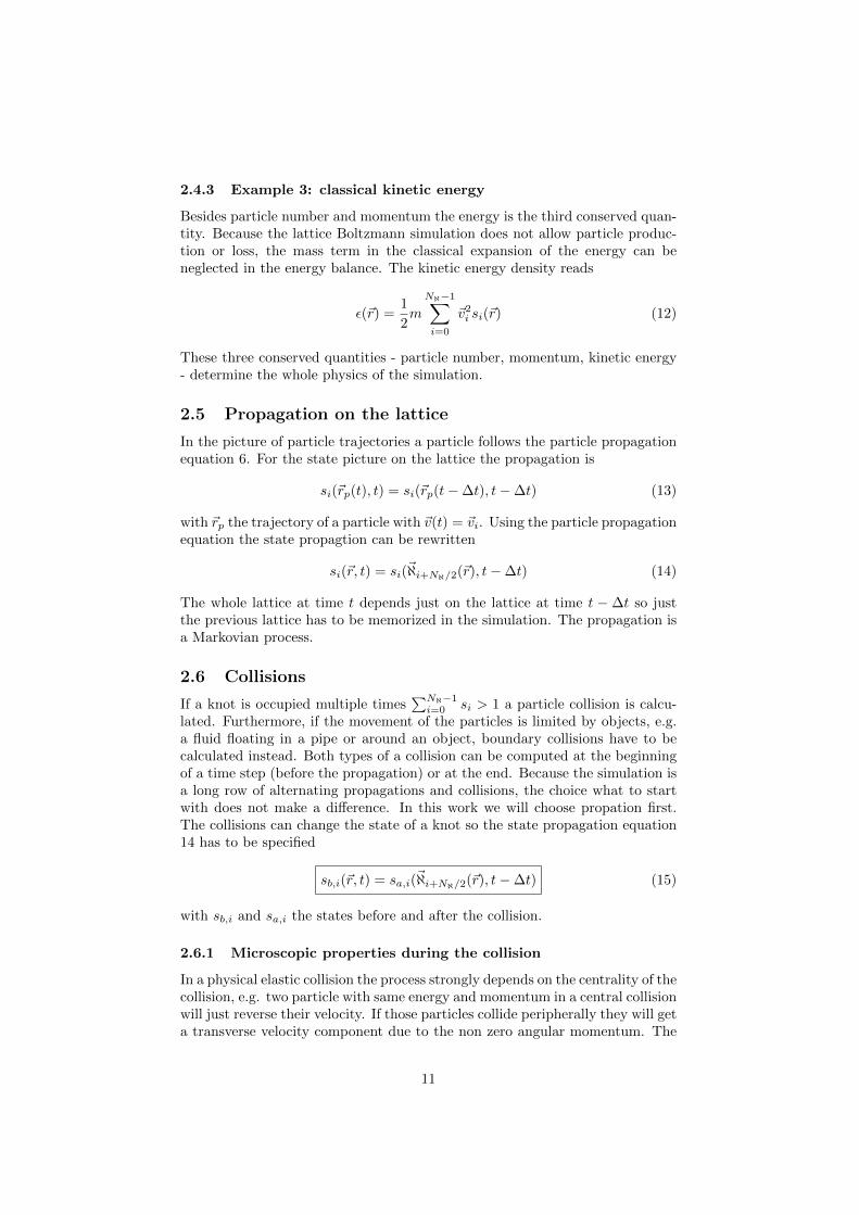
2.4.3 Example 3: classical kinetic energy

Besides particle number and momentum the energy is the third conserved quan-tity. Because the lattice Boltzmann simulation does not allow particle produc-tion or loss, the mass term in the classical expansion of the energy can beneglected in the energy balance. The kinetic energy density reads

ε(~r) =1

2m

Nℵ−1∑i=0

~v2i si(~r) (12)

These three conserved quantities - particle number, momentum, kinetic energy- determine the whole physics of the simulation.

2.5 Propagation on the lattice

In the picture of particle trajectories a particle follows the particle propagationequation 6. For the state picture on the lattice the propagation is

si(~rp(t), t) = si(~rp(t−∆t), t−∆t) (13)

with ~rp the trajectory of a particle with ~v(t) = ~vi. Using the particle propagationequation the state propagtion can be rewritten

si(~r, t) = si(~ℵi+Nℵ/2(~r), t−∆t) (14)

The whole lattice at time t depends just on the lattice at time t − ∆t so justthe previous lattice has to be memorized in the simulation. The propagation isa Markovian process.

2.6 Collisions

If a knot is occupied multiple times∑Nℵ−1i=0 si > 1 a particle collision is calcu-

lated. Furthermore, if the movement of the particles is limited by objects, e.g.a fluid floating in a pipe or around an object, boundary collisions have to becalculated instead. Both types of a collision can be computed at the beginningof a time step (before the propagation) or at the end. Because the simulation isa long row of alternating propagations and collisions, the choice what to startwith does not make a difference. In this work we will choose propation first.The collisions can change the state of a knot so the state propagation equation14 has to be specified

sb,i(~r, t) = sa,i(~ℵi+Nℵ/2(~r), t−∆t) (15)

with sb,i and sa,i the states before and after the collision.

2.6.1 Microscopic properties during the collision

In a physical elastic collision the process strongly depends on the centrality of thecollision, e.g. two particle with same energy and momentum in a central collisionwill just reverse their velocity. If those particles collide peripherally they will geta transverse velocity component due to the non zero angular momentum. The

11

lattice gas model does not contain information on the centrality of collisions.Instead, the Lattice Boltzmann simulation randomly chooses an outgoing state.In reference to section 2.3 there are 2Nℵ states S of a knot. The transfer fromstate S to state S′ in a collision can be described by a 2Nℵ × 2Nℵ probabilitymatrix A(S → S′). As the probability for S′ only depends on the S, the collisionis a Markovian process. Because after a collision the knot must be in any stateS′, the matrix fulfills ∑

S′

A(S → S′) = 1 ∀S (16)

If A(S → S′) ∈ 0, 1 ∀S, S′ the collision is deterministic and the whole develop-ment of the lattice gas is determined by its initial conditions. On a microscopicscale the simulation is chaotic so the deterministic case might be interesting tostudy for different initializations. But even for simple lattices that are used inthis work there is more than one outgoing state for an ingoing state in collision.These non-deterministic processes require deeper studying.

Collisions in a Lattice Boltzmann simulation usually obey the symmetry condi-tion called ”detailed balance”

A(S → S′) = A(S′ → S) ∀S, S′ (17)

Collisions with detailed balance are microreversible. The reversibility holds juston a microscopy scale; macroscopic processes e.g. gas expansion, can not bereverted. A weaker symmetry is ”semi-detailed balance”∑

S

A(S → S′) =∑S

A(S′ → S) ∀S′ (18)

The LHS can be interpreted as the total creation of S′ while the RHS expressesthe loss of S′, so probabilities for creation and loss are equal. Using equation16 the semi-detailed balance becomes∑

S

A(S → S′) = 1 ∀S′ (19)

which is the more common form.

The dual state S of a state S is defined be exchanging occupied and unoc-cupied directions in S (si → 1−si). As occupied directions represent a particle,an unoccupied state can be interpreted as a hole. The Lattice Boltzmann simu-lations is ”self-dual” if holes move like particles. The propagation equation (15)moves occupied and unoccupied states the same way and is thus self-dual. Thecollision is self-dual if

A(S → S′) = A(S → S′) ∀S, S′ (20)

With the detailed balanced condition the collision properbilities matrix A(S →S′) is symmetric and there are NA = 2Nℵ∗2Nℵ

2 + 2Nℵ

2 = 2 ∗ 4Nℵ−1 + 2Nℵ−1

matrix elements to determine. With the isotropy of the lattice previously dis-cussed there comes an invariance of the collision under rotation by angle 2π

N Nwith N ≥ 4 for a good isotropy and with self-duality the number od independent

12

matrix elements decreases even more.

Using equation 8 the conservation of collisional invariant O can be generalizedas

A(S → S′)

Nℵ−1∑i=0

oi(s′i − si) = 0 ∀S, S′ (21)

which means the probability is zero for a collision not conserving O and can be≥ 0 if conservation is satisfied. Such a possible state has to conserve particlenumber, momentum and energy. A simplification in the Lattice Boltzmannsimulation done is to assume an equal distribution of the probability among allpossible outgoing states S′ in a collision.

2.6.2 Collisions in the FHP models

In section 2.1.2 we found the two dimensional hexagonal lattice to be best suit-able for the simulation. Every knot has 6 neighbors and the states representparticles with these velocities (in lattice units)

~v0 =

(10

)~v1 =

(1/2

−√

3/2

)~v2 =

(−1/2

−√

3/2

)~v3 =

(−10

)~v4 =

(−1/2√

3/2

)~v5 =

(1/2√3/2

)In lattice units all particles have momentum ~pi = ~vi and energy ε = 0.5, soall particles can do in a collision is to change their direction i. The lattice hasa 2π

6 angular symmetry so the possible collisions can be rotated by 2π6 Z.

2.6.3 The FHP-1 model

The FHP-1 model contains 2 → 2 and 3 → 3 collisions as seen in figure 16 a)& b). The collisions conserve particle number, momentum and energy. TheFHP-1 model has this properties:

1. It is non-deterministic in 2→ 2 collisions.

2. The collision satisfies detailed balance.

3. It is not self-dual. The dual state of a 2→ 2 collision is a 4→ 4 collisionwhich is not included in the collision rules.

2.6.4 Modification of the FHP-1 model

The FHP-1 model can be improved to be more realistic by two modifications:The 4→ 4 collisions are added and A(S → S) 6= 0 is taken for all the collisions.The latter may look like no collision had happen but it should not be ignored. Ina real 2→ 2 collision with identical particles of same velocity a central collisionwill just invert the particle direction (cmp. fig. 16 a). In a 3 → 3 collisionthe process fig.16 b) just happens in a sufficient central collision. In a moreperipheral collision the ingoing particle state is obtained again. In the modifiedFHP-1 model the probabilities for the 2 → 2 and 3 → 3 transitions sink to1/3 resp 1/2. By including the S → S collisions and equally distributing theprobabilities for the different final states we obtain isotropy for the cross sections

13

as the probabilities are not depending on the direction of the outgoing particlesanymore. This model has following properties:

1. It is non-deterministic in all collisions.

2. The collision satisfies detailed balance.

3. It is self-dual.

Because the modified FHP-1 model is easy and efficient to handle with its 26 =64 states and small number of collisions, it is used in this work.

2.6.5 The FHP-2 model

The FHP-2 model is the FHP-1 model extended by a particle at rest withvanishing energy and momentum. The number of states per knot increases to128. The considered collisions are shown in figure 16.

Figure 16: Collision rules for the FHP-2 model with black dot as a particle atrest; figure taken from [6, p 45]

2.6.6 The FHP-3 model

If the FHP-2 model is extended by all possible collisions (except S → S) theFHP-3 model is obtained. The collisions are shown in figure 17

14

Figure 17: Collision rules for the FHP-3 model with black dot as a particle atrest. For all collision rules apply self-duality. Figure taken from [6, p 49]

The FPH-3 model has following properties

1. It is non-deterministic in most collisions.

2. The collision satisfies detailed balance.

3. It is self-dual. This is the major improvement to FHP-1 and FHP-2.

2.6.7 Collisions on square lattices

The simplest model on a square lattice is the HPP model as shown in figure 19a) with just four neighbors per knot and the velocity vectors

15

~v0 =

(10

)~v1 =

(0−1

)~v2 =

(−10

)~v3 =

(01

)Only head on head two particle collisions are possible (cmp. fig. 18).

Figure 18: Collision rules of the HPP model reduced by rotational symmetryfigure taken from [6, p. 36]

The HPP model has the handy properties

1. It is deterministic.

2. The collision satisfies detailed balance.

3. It is self-dual.

On the downside this model has an insufficient π/2 isotropy discussed in 2.1.2,so we have to introduce more neighbors. A good compromise between the sim-ple HPP and the complex model in figure 19 b) is the eight neighbors squarelattice model (8NSL model) introduced in section 2.1.2. It has eight velocities

~v0 =

(10

)~v1 =

(1−1

)~v2 =

(0−1

)~v3 =

(−1−1

)~v4 =

(−10

)~v5 =

(−11

)~v6 =

(01

)~v7 =

(11

)

16

Figure 19: a) HPP model, b) more complex square model; figure taken from[6, p. 25]

Though this model has the same π2 rotational symmetry as the HPP, it has a

π4 angular isotropy. The states can be divided into classes of absolute velocity

1 (velocities in x or y direction, even direction index i) and√

2 (diagonal veloc-ities, odd direction index i). Each class can perform the head on head collisionknown from HPP with the S → S process for central collisions. Furthermore, theclasses can interact in many different collisions. If we denote S = (s0, s1, ..., s7)than 2 particle collisions such as (1, 0, 0, 1, 0, 0, 0, 0) → (0, 1, 0, 0, 1, 0, 0, 0) or 3particle collisions (1, 0, 1, 0, 0, 1, 0, 0)→ (0, 0, 1, 0, 1, 0, 0, 1) and others are possi-ble. The collisions must satisfy

1. The model is non-deterministic in all collisions.

2. The collisions satisfy detailed balance.

3. It is self-dual.

2.6.8 Boundary collisions

In order to simulate walls, borders and solid, not traversable objects a reflectionof particles must be integrated into the models. For this we define a specialboundary collision that is performed at knots that define the surface of the ob-ject instead of the ordinary particle collision. These collisions must guaranteethat no particle gets inside the object so the inside knots remain empty. In aphysical collision with a boundary at rest some momentum is transfered to theboundary to keep the total momentum conserved resulting in a slowly movingboundary. As we take the knots for fixed in space in the Lattice Boltzmannsimulation, the momentum is not conserved in boundary collisions. Particlenumber and energy are conserved. Figure 20 shows three of the several existingreflection models.

17

The bounce-back reflection inverts the momentum of an incoming particle (px, py)→(−px,−py). This reflections works locally as in the state picture we can use thepoint-symmetry of direction indexes to write

si → si+Nℵ/2 (22)

The specular reflection reflects particles like a perfect mirror reflects light. Themomentum parallel to the surface is conserved while the orthogonal componentis inverted (p⊥, p‖) → (−p⊥, p‖). Because this boundary collision model needsto know the orientation of the surface, it can not be calculated locally but theknot needs information of its neighbors. To make this problem pseudo-local wecan give the orientation of the surface at a knot as additional information tothe knot.

The diffusive reflection is a combination of bounce-back and specular reflec-tion. For every collision randomly one of these reflection models is chosen.

Figure 20: Three simple reflection models; figure taken from [6, p. 31]

2.7 Sources/sinks of observables

In some scenarios one wants to include sources or sinks, where the amount of anobservable quantity is increased or decreased. This can be realized by definingsource/sink collision that replace the ordinary collisions at the desired place.The source/sink collision is basically determined by the observables conservedand the ones to in-/decrease. An example is a local heating that conservesparticle number and momentum but increases the energy. The latter requiresdifferent velocities. In the 8NSL model a heating is realized by by transferringv = 1 particle to v =

√2 ones. In head on head collisions this is e.g. S =

18

(1, 0, 0, 0, 1, 0, 0, 0) → S′ = (0, 1, 0, 0, 0, 1, 0, 0). The intensity of the heating isadjusted by tuning the collision probabilities for energy increasing processes.

2.8 Defintion of lattice units and conversion from and tophysical units

The physical input quantities, such as mass m , measures of the lattice, Boltz-mann constant kB , and quantities derived from them, e.g. duration of a timestep ∆t, velocities ~v , knot distances ∆~l, are needed for the probability com-putation in initialization and or the post-processing but not for the evolution.For simplicity we can introduce lattice units. At the beginning we convert therelevant quantities to lattice units and at the end of the post-processing backto physical units. For the velocities we define a value vtyp, e.g. the smallestabsolute velocity and express velocities in term of vtyp. A physical velocity ~vcan then be expressed with the dimensionless lattice velocity ~vl as ~v = vtyp~v

l.

With ∆~l = ~v∆t we can express knot distances in units of vtyp∆t so ∆~ll = ~vl

The temperature appears in the equipartition theorem and in distribution, e.g.Maxwell-Boltzmann or Dirac, so it is handy to define the temperature T l inlattice units

T l = TkB

mv2typ

(23)

Furthermore, we can set ml = ∆tl = 1. The equipartition theorem simplifies inlattice units to

Tx = 〈v2x〉 − 〈vx〉

2(24)

with the lattice units index l dropped.

19

3 Conceptional problems of the Lattice Boltz-mann simulation

3.1 Fluid cells on a lattice

In hydrodynamic modeling a fluid is split in fluid cells each of which charac-terized by the densities of thermodynamic quantities. Those cells meets tworequirements

1. Each cell has to contain enough particles for proper statistics so localthermodynamic quantities can be defined.

2. Each cell has to be small enough to ensure approximate homogeneity sothe thermodynamic quantities do not vary too much inside a cell.

In real physics, even for a gas with typically a O(107/µm3) particle density,these requirements are no problem. In the simulation one knot is ways toosmall for a fluid cell; round about a thousand (at least once occupied) knotsper cell are necessary for a sufficient statistical basis. On e.g. an 1000 × 1000lattice quantities show significant variation on 10 to 20 knot distances whichis why good statistics can not be obtained on the lattice fluid cells. Anotherproblem is the spacial resolution of the lattice e.g. with cells of 20×20 knots ona 1000×1000 lattice one would get the equivalent to a picture of the observabledistribution with just 50 × 50 pixels. The latter problem can by solved bydropping the concept of splitting the fluid in cells. Instead a cell can be definedaround every knot. With those overlapping fluid cells the resolution of thesimulation is simply the number of knots used. But the overlapping fluid cellsstill have to be small so we expect low precision in the observables. An errorcomputation is obligatory. To obtain valuable results one has to average overmultiple lattice simulations.

3.2 Smooth boundaries in discrete space

The specular reflection is the physical most correct model but it depends onthe orientation of the surface which is not obvious. The knots are discretein space so smooth surfaces can often not be realized with the very limitednumber of directions i the model offers so the position of surface knots has tobe approximated. In these cases the a vector ~R‖ parallel to the surface can becalculated as

~R‖ = ∆t∑

~vi(~r)∈Ω

~vi(~r) (25)

with Ω containing all velocity vectors ~vi(~r) from one surface knot to the nextone. An alternative is to define a set of reflection planes, e.g. parallel to ~viand to approximate a smooth surface with these planes. This method requiresevery knot to know its reflection plane. Even with these methods we can notalways define a reflection plane, e.g. for a knot at the corner of an object thereexists no clear reflection plane. In this case the bounce-back reflection is thebest choice.

20

3.3 Equipartition theorem in the FHP-1 model

The FHP-1 model has only one value v for the velocity what becomes a problemduring the simulation. If we have a point-symmetric initial temperature distri-bution with respect to some knot (the ”center” of the fluid), we automaticallyget a point symmetric particle and velocity distribution with 〈~v(t = 0)〉 = ~0.For symmetry reasons we expect 〈~v(t > 0)〉 = ~0 so the lattice is always the lo-cal rest frame for the particles at the center. With isotropic temperatures theequipartition theorem simplifies to

kBT =1

2m 〈~v2〉 =

1

2mv2 (26)

As v is a constant during the whole simulation the temperature is fix in contrastto the physical reality.In the anisotropic case we obtain two equipartition equations

1

2kBTx =

1

2m 〈~v2〉x =

1

2mv2Nx + cos2(π/3)Nd

Nx +Nd

1

2kBTy =

1

2m 〈~v2〉y =

1

2mv2 sin2(π/3)Nd

Nx +Nd

(27)

withNx andNd the number of particles with horizontal resp. diagonal velocities.The equations depend linear on each other:

1

2kBTx =

1

2mv2

(1− sin2(π/3)Nd

Nx +Nd

)=

1

2mv2 − 1

2kBTy (28)

The linearity is, per se, an unrealistic phenomenon. In addition we expect thetemperatures to align over time and Tx → Ty reproduces the isotropic concep-tional problem again. In the FHP-1 model we have to declare the equipartitiontheorem invalid for t > 0. After the initialization at t = 0 the used distribution(e.g. Maxwell, Fermi, Bose-Einstein distribution) remains the only valid defi-nition of the temperatures. In the hexagonal model the distribution ρN,03 ofparticles in pure x direction (with velocity ~v0 or ~v3)only depends on Tx and noton Ty so it can be used to calculate a value for Tx. With Tx fixed (for the knotand time step) the distribution ρN,1245 of particles with diagonal velocities hasjust the temperature in y direction as unknown variable and can be solved forTy.

3.4 Energy conservation in FHP-2 and FHP-3

In the FHP-2 model the collisions e) and f) on figure 16 change energy by ∆ε =0.5 resp. ∆ε = −0.5. Even though on the microscopic scale the energy is notconserved, the collisons can be used if energy is conserved macroscopically. For asimulation with isotroic temperatures that might least if e) and f) hold balance.For anisotropic temperatures the collisions are not in balance what can easily beseen on a lattice with Tx > Ty: The thermodynamically most expected particlesare resting; there is a medium amount of particles in ±x-direction (horizontal)and particles with diagonal velocities are more rare. Because collision f) alwaysneeds at least one of the rare diagonal particles while collision e) works with thevery common resting paricles and any ~v 6= ~0, collision e) happens more often

21

than collision f). The total energy on the lattice increases so these collisions cannot be used here.Collisions c) and d) are the equivalent of a) and b) with a resting particle thatdoes not move or influence the process. In conclusion the resting particles andthe moving ones are decoupled and can be seen as two lattices: One works likeFHP-1 and the one with the resting particles is static and contributes to thesimulation as constants added to the observables.In the FHP-3 model collisions b)to g) in figure 17 do not conserve energy onthe microscopic scale. With an argumentation simular to the one for FHP-2 wefind that total macroscopic energy conservation is violated again.Only the (modified) FHP-1 model can be used for anisotropic temperatures. Tofind other usable models the one can introduce more neighbor relations (andmore velocities) on the hexagonal lattice (e.g. the GBL model) or use anotherlattice.

22

4 Implementation of a Lattice Boltzmann sim-ulation

A Lattice Boltzmann simulation can be implemented with no need for object-orientation or analytic functionality. A programming language with efficientnumerics, e.g. c or Fortran, is the best choice. For initialization and collisionsa good random number generator is needed; in this work the Mersenne Twisterby Takuji Nishimura and Makoto Matsumoto, Hiroshima-University, is used.For the calculation a normal PC is enough. Depending on the precision andthe lattice size 0.5GB free RAM is needed for a 1000 × 1000 lattice, 2GB for2000× 2000 etc.

4.1 Storing the lattice configuaration

To store the boolean states si(~r) of a lattice configuration arrays can be used intwo ways: A bitwise storage scheme stores the states of different knots in onearray per direction i. Alternatively one can create an array per knot that storesstates of all directions. Modern programming languages support multidimen-sional arrays so there is no more need to number the knots. Instead one canrecall the definition of Bravais lattices (5) to project any lattice on the squarelattice that is usually implied by an multidimensional array: In n-dimensionalspace each knot is stored in a n-dimensional array entry accessible by the coor-dinates li. To store the different states for the si an extra dimension is needed.As the neighbor relations can be more complicated (as discussed in section 2.1)it is recommended to write a function giveNeighbor : (i, l1, l2, ...) → (l′1, l

′2, ...)

that gives the coordinates l′i of a knots neighbor in direction i. While a Bravaislattice in infinitely large, a simulated lattice has to be finite. There are threecommon ways to threat the borders:

1. Boundary borders: If the borders of the lattice are defined as boundariesthe particles are reflectet back towards the inner of the lattice. Particlenumber and energy are conserved but not the momentum as previouslydiscussed. This model correspond to a fluid in a box.

2. Periodic borders: To describe the physics on a torus, one has to rewritethe giveNeighbor function so it includes knot at one end of the latticeas neighbors of the other end. This way particle number, energy andmomentum are conserved.

3. Open borders: If the borders are left open, particles can leave the simula-tion. The idea is that the interesting processes happen in the center. Theparticles far away have little influence on the center because their chanceto come back to the center is low so they can be removed. In an opensystem the global conservation laws become invalid.

The states can be stored like this in the simulation. For precise results one hasto average over multiple Lattice Boltzmann simulations; Nsim = 20 simulationsturn out to be enough to get smooth diagrams. The easiest and most flexible(concerning post processing) way is to simulate and store all lattice configura-tions in parallel. To save memory one can alternatively perform the simulationsone after the other and store the extracted observables separately. In order to

23

enhance the memory access to the lattice storage array elements one should beaware of the array index order:

l a t t i c e S t o r a g e A r r a y [ N sim ] [ l 1 ] [ l 2 ] . . . [ d i r e c t i o n i ]

This array is needed twice: for the lattice of the time step t and for the previouslattice at t− 1.

The simulation consists of three parts: initialization, the evolution and thepost processing.

4.2 Initialization of the lattice

With the lattice size, the knot number, the temperatures, the particle mass andthe particle number/density given the lattice is completely determined. Theinitialization has four steps:

1. Calculation of the typical velocity vtyp

2. Calculation of the distribution with the typical velocity

3. Normalization of the distribution

4. Filling the lattice with particles according to normalized distribution

Denote the used distribution (here: Maxwell-Boltzmann distribution) asf(m, vtyp, ~vi, Tx, Ty) with ~vi the velocity in lattice units. The equipartitiontheorem can be rewritten as

1

2kBTx =

1

2mv2

typ

∑Nℵi=0(~vi~ex)2f(m, vtyp, ~vi, Tx, Ty)∑Nℵ

i=0 f(m, vtyp, ~vi, Tx, Ty)(29)

The (~vi~ex)2 projects the velocity at the x direction. The denominator is neededbecause f is a spatial distribution and not normalized yet. The equation cannot be solved analytically for vtyp but numerically. With the value for vtypthe distribution terms can be evaluated. The probability Pi for state si to beoccupied is

Pi(~r) = NNorm(~r)f(m, vtyp, ~vi, Tx, Ty) (30)

Because we want to obtain a given particle density ρN (~r) (per knot) as expec-tation value, the condition

ρN (~r) =

Nℵ∑i=0

Pi(~r)

⇒ NNorm(~r) =ρN (~r)∑Nℵ

i=0 f(m, vtyp, ~vi, Tx, Ty)

(31)

holds. From this equation one can see the particle density ρN has to be smallerthan Nℵ in order to obtain Pi < 1. The Maxwell-Boltzmann-Distribution onlyworks for low particle densities so we just have ρN Nℵ.With the probabilities calculated we can loop over the simulations, coordinatesand directions and use a random number generator uniform in [0, 1] to set si.

24

4.3 Evolution of the lattice

The evolution takes place in a time loop of propagation and collisions that bothhave been discussed previously. The collisions can be implemented in two ways:Using if statements in simple models such as FHP and HPP the collisions canprogrammed by hand. For more complex models it is more efficient to use thecollision probability matrix A(S → S′) as a look-up table. The latter can beautomatically created. Because the conditions for allowed collisions (conserva-tion of particle number, energy, momentum) are simple sums and differencesand can be computed quickly, one can calculate the upper triangular matrixwithout using self-duality and rotational invariance.

4.4 The post-processing

During the initialization we went from the macroscopic thermodynamical de-scription of the fluid to the microscopic simulation on the lattice. The post-processing is the reverse process at a later time. The post-processing happensin two steps:

1. raw lattice data extraction

2. computation of observables

As we do not store the complete time evolution of the lattice, the raw dataextraction has to happen at the right time step and position during the evolutionof the lattice. The computation of the observables can happen whenever afterthat, but if it is done right after the extraction we can save the memory wewould otherwise need to store the raw data.

4.4.1 Raw lattice data extraction

In thermodynamics the macroscopic relevant quantities are obtained by an aver-aging process. Because of statistical deviations the quantities are a little noisy.On the lattice averaging can be done in basically two ways:

4.4.1.1 Ensemble-averaging extractionThe method of ensemble-averaging can be used if the simulation is run multipletimes with the same macroscopic conditions (same initial probabilities etc.). Byaveraging at one selected knot and time step over all the simulations the requireddata can be extracted with high precision. The advantage of this method is thehigh resolution in time and space - data is exactly extracted at one point andone time. On the downside this method consumes much computing power as itneeds to run hundreds of simulations.An useful value to extract is the ratio of particles nvi with velocity ~vi to allparticles at the knot. In ensemble-average it is

nvi (~r) =1

Nsim

Nsim∑lbs=1

si(~r, lbs)∑Nℵj=0 sj(~r, lbs)

(32)

with si(~r, lbs) the state si(~r) in Lattice Boltzmann simulation number lbs.

25

4.4.1.2 Space- and time-averaging extractionOn just one lattice we can define a small region V in space-time containing NVknots. When averaging over V the resolution decreases but the extracted valuesget less noisy. One must be aware that the system might undergo significantchanges within V if it is chosen too large. E.g. the particle ratio in space-/time-averaging is

nvi (~r) =1

NV

∑(t,~r)∈V

si(t, ~r)∑Nℵj=0 sj(t, ~r)

(33)

4.4.1.3 Averaging over fluid cellsOverlapping fluid cells introduced in section 3.1 are a combination of ensemble-and space-averaging. On a 1000×1000 lattice a 50×50 fluid cells 20 times sim-ulated is a good compromise between spacial resolution and low computationalcosts.

nvi (~r) =1

NsimNV

Nsim∑lbs=1

∑(t,~r)∈V

si(t, ~r, lbs)∑Nℵj=0 sj(t, ~r, lbs)

(34)

We receive similar terms for other ratios. The other important raw quantity weextract is 〈si(~r)〉.

4.4.2 Computation of observables

With the extracted ratios average values for quantities can be calculated, e.g.

〈vx〉 =

Nℵ∑i=0

(~vi~ex)nvi

〈v2x〉 =

Nℵ∑i=0

(~vi~ex)2nvi

(35)

In lattice units the temperature reads

Tx =

Nℵ∑i=0

(~vi~ex)2nvi −

(Nℵ∑i=0

(~vi~ex)nvi

)2

(36)

The extracted average occupations 〈si〉 can be used to calculate observables inequation(8). The calculated observables can now be stored for further process-ing, e.g. plotting with external software like gnuplot or Origin.

26

5 Results of the simulations using modified FHP-1 and 8NSL models

5.1 The FHP-1 model: radial expansion of a circle shapedfluid in vacuum

As a test for the implemented FHP-1 model a uniform fluid was initialized withina circle of size 122.718 GeV−2 = 4.778fm2 around the center of the 1000×1000lattice that covers an area of 50 GeV−1× 50 GeV−1. With initial temperaturesTx = 0.01 GeV, Ty = 0.05 GeV and a mass m = 1.8 GeV. The development ofthe temperature in the center is shown in figure 21:

0

0.01

0.02

0.03

0.04

0.05

0.06

0 500 1000 1500 2000 2500 3000 3500 4000

tem

pera

ture

[G

eV

]

time [GeV-1]

centre: Txcentre: Ty

Figure 21: Temperatures at the center of the initial volume

The development over the whole time shown looks quite realistic; for the simu-lation of isotropic temperatures the FHP-1 model is a fast and efficient approx-imation. But the alignment of Tx and Ty happens in just one time step. Toincrease the time resolution we can increase the number of knot on the latticebecause ∆t = |∆~li|

|~vi| . Figures 22 and 23 showing the first five time steps on a

1000× 1000 resp 2000× 2000 lattice (with linear interpolation) have lost all in-formation on anisotropy within the first time step. With only one velocity valuethe FHP-1 model turns out to be too simple for a Lattice Boltzmann simulationwith anisotropic temperatures.

27

0

0.01

0.02

0.03

0.04

0.05

0.06

0 0.2 0.4 0.6 0.8 1 1.2

tem

pera

ture

[G

eV

]

time [GeV-1]

centre: Txcentre: Ty

Figure 22: Temperatures at the center of a 1000× 1000 lattice

0

0.01

0.02

0.03

0.04

0.05

0.06

0 0.1 0.2 0.3 0.4 0.5 0.6

tem

pera

ture

[G

eV

]

time [GeV-1]

centre: Txcentre: Ty

Figure 23: Temperatures at the center of a 2000× 2000 lattice

5.2 The 8NSL model: radial expansion of a circle shapedfluid in vacuum

As the FHP-1 model loses information on anisotropy too fast, another modelhas to be implemented to achieve a realistic approach to isotropy. To test theimplemented eight neighbor square lattice model a uniform fluid was initializedwithin a circle of size as discussed for the FHP-1 model. The 8NSL model isprecise enough to simulate the alignment process of Tx and Ty.

28

0

0.002

0.004

0.006

0.008

0.01

0.012

0.014

0.016

0.018

0.02

0 20 40 60 80 100 120

tem

pera

ture

[G

eV

]

time [GeV-1]

center: Txcenter: Ty

Figure 24: Temperature development in the center of a 1000× 1000 lattice

For later times the particle density at the center decreases too low for goodstatistics that is shown in figure 24 with large error bars. With larger latticeswe obtain even better time resolution for the alignment but the 1000 × 1000lattice can be seen as sufficient precise for further simulation.

0

0.002

0.004

0.006

0.008

0.01

0.012

0.014

0.016

0 5 10 15 20

tem

pera

ture

[G

eV

]

time [GeV-1]

center: Txcenter: Ty

Figure 25: Temperature development in the center of a 2000× 2000 lattice

The distribution profile along the horizontal line element from the center (25, 25) GeV−1

to the edge at x = 50 GeV−1 in figure 26 shows an artifact of the measurement

29

0

0.1

0.2

0.3

0.4

0.5

0.6

0.7

25 30 35 40 45 50

part

icle

dis

trib

uti

on [

per

knot]

x-position [GeV-1]

xDistributionyDistribution

xyDistribution

Figure 26: distribution profile at t = 0

method: As the fluid is initialized uniform within the initialization circle withvacuum outside, the profile at t = 0 should make a step at x = 31.25 GeV−1.The linear decrease is caused by the spacial averaging (cmp. section 4.4.1.3)as latter contains initial and non-initial volume for knots near the edges. Att = 120 shown in figure 27 only particles in x direction have propagated in theprofile. Within the initial volume some particles with other velocities are left.The particles outside linearly propagate without collisions. They form a shockwave with its maximum/front at x = 35.5GeV−1.

0

0.05

0.1

0.15

0.2

0.25

0.3

0.35

0.4

25 30 35 40 45 50

part

icle

dis

trib

uti

on [

per

knot]

x-position [GeV-1]

xDistributionyDistribution

xyDistribution

Figure 27: distribution profile at t = 120

30

5.2.1 Time evolution of the particle distribution

To examine the particle movement over time, the particle number density in2D space is plotted for different time steps. In figure 28 the fluid has radiallyexpanded. But first breaks of radial isotropy can be seen. As time goes by thoseisotropy breaks get extreme as seen in figure 29. This distribution is unphysicaland a pure artifact of the model used.

0

5

10

15

20

25

30

35

40

45

50

0 5 10 15 20 25 30 35 40 45 50

y-p

osi

tion [

GeV-1

]

x-position [GeV-1]

particleDistribution

0

0.2

0.4

0.6

0.8

1

1.2

1.4

1.6

1.8

part

icle

dis

trib

uti

on [

per

knot]

Figure 28: particle distribution at t = 60

0

5

10

15

20

25

30

35

40

45

50

0 5 10 15 20 25 30 35 40 45 50

y-p

osi

tion [

GeV-1

]

x-position [GeV-1]

particleDistribution

0

0.05

0.1

0.15

0.2

0.25

0.3

0.35

0.4

0.45

0.5

part

icle

dis

trib

uti

on [

per

knot]

Figure 29: particle distribution at t = 200

31

Figures 30 and 31 show particles leaving the initialization circle (with radiusr = 6.25 GeV−1). Around the x axis there are only particles with velocityin ±x-direction, analogically for y and diagonals. Those free flying particlesundergo no collision due to the model that only has one velocity value for eachdirection. This causes the eight directions characterizing the 8NSL-model todominate the particle distribution for large times (fig 29).

0

5

10

15

20

25

30

35

40

45

50

0 5 10 15 20 25 30 35 40 45 50

y-p

osi

tion [

GeV-1

]

x-position [GeV-1]

X particle Distribution

0

0.1

0.2

0.3

0.4

0.5

0.6

0.7

0.8

part

icle

dis

trib

uti

on [

per

knot]

Figure 30: Distribution of particles with velocity in x direction at t = 60

0

5

10

15

20

25

30

35

40

45

50

0 5 10 15 20 25 30 35 40 45 50

y-p

osi

tion [

GeV-1

]

x-position [GeV-1]

diagonal particle Distribution

0

0.02

0.04

0.06

0.08

0.1

0.12

part

icle

dis

trib

uti

on [

per

knot]

Figure 31: Distribution of particles with velocity in diagonal direction at t =60

32

5.2.2 Time evolution of the temperature field

The radial isotropy breaks seen in the particle distribution appear in the tem-perature field again.

0

5

10

15

20

25

30

35

40

45

50

0 5 10 15 20 25 30 35 40 45 50

y-p

osi

tion [

GeV-1

]

x-position [GeV-1]

0

0.001

0.002

0.003

0.004

0.005

0.006

0.007

0.008

0.009

tem

pera

ture

[G

eV

]

Figure 32: Maximum of Tx and Ty at t = 60

0

5

10

15

20

25

30

35

40

45

50

0 5 10 15 20 25 30 35 40 45 50

y-p

osi

tion [

GeV-1

]

x-position [GeV-1]

0

0.001

0.002

0.003

0.004

0.005

0.006

0.007

0.008

0.009

tem

pera

ture

[G

eV

]

Figure 33: Maximum of Tx and Ty at t = 120

33

0

5

10

15

20

25

30

35

40

45

50

0 5 10 15 20 25 30 35 40 45 50

y-p

osi

tion [

GeV-1

]

x-position [GeV-1]

0

0.001

0.002

0.003

0.004

0.005

0.006

0.007

0.008

0.009

tem

pera

ture

[G

eV

]

Figure 34: Maximum of Tx and Ty at t = 200

The T = 0 in horizontal and vertical direction from the center are an artifact ofthe free particle flow. The latter have not temperature due to 〈v2〉 = 〈v〉2. Asthe particles in diagonal direction are flying freely they cannot contribute to thesmall temperatures in the diagonal directions. Figures 30 and 31 that particlesdistributions from different axes slightly overlap so a small amount of particlesfrom another axis can cause collisions and create a small finite contribution to〈v2〉 − 〈v〉2. As the particle density in horizontal and vertical directions is afactor 10 larger than in diagonal direction, the contributions have a smallereffect on horizontal/vertical than on diagonal temperature field.

5.2.3 Comparison with continuum simulation

To compare the results of the Lattice Boltzmann simulation to the simulationby G.A. Bird, the temperature profile along the horizontal axis from the centerhas been plotted in figure 35 and 36. The parallel temperature Tx outside theinitialization circle quickly declines to 0 as an effect of the free particle flight.The orthogonal temperature Ty has two stages: The one far from the center isexpected as the simulated scenario is a shock wave emission. The other stagestarts just outside the initialization circle and is an unphysical artifact. Forlarge times the latter stage develops the form of a curve.

34

0

0.001

0.002

0.003

0.004

0.005

0.006

0.007

0.008

0 5 10 15 20 25

tem

pera

ture

[G

eV

]

x-position [GeV-1]

x temperatureorthogonal temperature

Figure 35: Temperature profile along horizontal axis at t = 60

0

0.0002

0.0004

0.0006

0.0008

0.001

0.0012

0 5 10 15 20 25

tem

pera

ture

[G

eV

]

x-position [GeV-1]

x temperatureorthogonal temperature

Figure 36: Temperature profile along horizontal axis at t = 200

G.A. Bird’s simulation of the same problem leads to plot 37. Before the firststage in the center (where the particle density is high and the scaled mean freepath length P small) both diagrams correspond with Tx/Ty ≈ 1. At the firststage the ratio jumps to Tx/Ty ≈ 2. At the second stage of Ty the particlesin horizontal direction have reached free flight (P → ∞) so the temperaturevalue Tx = 0 loses physical meaning. These two artifacts make it hard todo a meaningful comparison but broadly approximated the diagrams of both

35

Figure 37: temperature ratio Tx/Ty profile depending on the scaled mean freepath length P [2]

continuous simulation and the Lattice Boltzmann simulation correspond as theyshow the same trend for Tx/Ty.

5.3 Prospects of Lattice Boltzmann simulation with anisotropictemperatures

The FHP-1 model turns out to be too simple to be sufficiently precise for thesimulation of anisotropic temperature development. More advanced models onthe hexagonal lattice, e.g. the GBL model [6, p. 53] with 3 velocitiy values,might work but will increase complexity and needed computation power as adownside.The 8NSL model provides a good time resolution of the isotropization processbut the discussed artifacts dominate the outer regions of the temperature field.The model can approximate the real fluid within twice the initialization radiusri. As we do not need to simulate r > 2ri the initialization radius can beenlarged (concerning the number of knots inside ri) to obtain a finer discretizedspace. Contrary to the expectations simulations show that a larger initializationcircle (by factor four) does not dampen the development of artifacts. For preciseresults a more complex model (e.g. figure 19 b) is needed at the price of highercomputation duration. A model with more than one velocity value in eachdirection would suppress the free stream of particles outside the initialization

36

circle by producing collisions there and avoid the zero temperature problem aswell as the anisotropic particle distribution in the expanding fluid. Nevertheless,the 8NSL model provides a acceptable approximation for anisotropic fluids andcan be applied in other scenarios than expanding gas balls. But this is work foranother thesis.

37

References

[1] A. Miffre, M. Jacquey, M. Buchner, G. Trenec , J. Vigue. Parallel tempera-tures in supersonic beams: Ultra cooling of light atoms seeded in a heaviercarrier gas. 2008. http://arxiv.org/abs/physics/0406124v3.pdf; ac-cessed 20-August-2015.

[2] G.A. Bird. Breakdown of translational and rotational equilibrium in gaseousexpansions. AIAA journal, 8:1998, 1969.

[3] N. Borghini. Elements of Hydrodynamics. Bielefeld University,2015. http://www.physik.uni-bielefeld.de/~borghini/Teaching/

Hydrodynamics/Hydrodynamics.pdf; accessed 22-July-2015.

[4] Czycholl. Theoretische Festkorperphysik. Springer, third edition, 2008.

[5] Nicolas Borghini, Steffen Feld, Christian Lang. Kinetic freeze-out from ananisotropic fluid in high-energy heavy-ion collisions: particle spectra, han-bury browntwiss radii, and anisotropic flow. The European physical journal,75:275, 2015.

[6] Rivet and Boon. Lattice Gas Hydrodynamics. Cambridge University Press,2001.

38

Eigenstandigkeitserklarung

Ich versichere hiermit, dass ich die vorstehende Masterarbeit mit dem Titel:

”Approach to and departure from local isotropy in Lattice Boltzmann simu-lations”

selbststandig verfasst und keine anderen als die im Literaturverzeichnis angegebe-nen Hilfsmittel benutzt habe. Die Quellen der benutzten Grafiken habe ichangegeben.

(Unterschrift Tobias Mohrmann)

39