Master Thesis Neighbor Discovery and ... - pub.tik.ee.ethz.ch · Acknowledgments The master’s...
116
Spring Semester 2009 Prof. Dr. Lothar Thiele Master Thesis Neighbor Discovery and Topology Construction of Wireless Sensor Networks Aldo Bazzi Supervisors: Dr. Simon K¨ unzli (Siemens BT) Dr. Andreas Meier (ETH) Dr. Jan Beutel (ETH)
Transcript of Master Thesis Neighbor Discovery and ... - pub.tik.ee.ethz.ch · Acknowledgments The master’s...

Spring Semester 2009 Prof. Dr. Lothar Thiele
Master Thesis
Neighbor Discovery and Topology
Construction of Wireless Sensor Networks
Aldo Bazzi
Supervisors:
Dr. Simon Kunzli (Siemens BT)
Dr. Andreas Meier (ETH)
Dr. Jan Beutel (ETH)


Acknowledgments
The master’s thesis presented in this report was made in response of a thesis
proposal from the Computer Engineering and Networks Laboratory (TIK)
at the Swiss Federal Institute of Technology (ETH) Zurich in collaboration
with the Communication and Wireless Group (CWL Group) of Siemens
Building Technologies (BT) in Zug.
I would like to thank my advisors Dr. Simon Kunzli, Senior Engineer
at Siemens BT Zug, Dr. Andreas Meier, research assistant at ETH Zurich,
and Dr. Jan Beutel, senior researcher at ETH Zurich for supervising my
work and for their great and helpful support during my master’s thesis.
I would also like to thank Siemens BT for the opportunity to pursue my
master’s thesis in the interesting area of wireless fire detection systems and
the whole CWL Group for their support and the comfortable atmosphere
during my work.
Zug, 20 October 2009
Aldo Bazzi
III

IV

Abstract
In this thesis the new procedure Mesh Construct for neighbor discovery
and mesh topology construction of radio alarm systems based on multihop
wireless sensor networks (WSNs) is presented.
The detectors of such a system are equipped with a radio transceiver
and a pack of batteries in order to report detected dangers wirelessly over
possibly multiple hops to a central node of the underlying multihop WSN.
To ensure a reliable alarm message transmission several node-disjoint multi
hop routing paths from each detector to the central station are required.
A connectivity state is defined to determine whether the constructed mesh
network fulfills this requirement.
The Mesh Construct procedure constructs a mesh network topology by
initiating neighborhood discoveries on each node starting from the central
station and proceeding outwards hop by hop. During the neighborhood
discoveries nodes are chosen as neighbors depending on the link quality and
a possible connectivity state improvement.
After the completion of the Mesh Construct procedure the operation of
the radio alarm system including a topology control procedure is started.
Removals of inappropriate neighbors by the topology control can cause in-
stabilities in the connectivity state of the network and increase energy con-
sumption.
The objective of the Mesh Construct is to discover neighbors and con-
struct a stable mesh network topology in terms of connectivity in a fast and
energy-efficient way.
The evaluation of performed Mesh Construct tests showed promising re-
sults. Compared to an existing solution with the Mesh Construct procedure
the energy consumption, the duration, and the network instability could be
reduced.

VI
Master’s Thesis CONTENTS
Contents
List of Figures X
List of Tables XIII
1 Introduction 1
1.1 Setup . . . . . . . . . . . . . . . . . . . . . . . . . . . . . . . 2
1.1.1 Definitions . . . . . . . . . . . . . . . . . . . . . . . . 2
1.1.2 Multihop Wireless Fire Detection Sensor Network at
Siemens BT . . . . . . . . . . . . . . . . . . . . . . . . 6
1.2 Problem Description . . . . . . . . . . . . . . . . . . . . . . . 7
1.2.1 Neighbor Discovery and Topology Construction . . . . 7
1.2.2 Requirements and Assumptions . . . . . . . . . . . . . 9
1.2.3 Quality Metrics and Objectives . . . . . . . . . . . . . 10
1.3 Chapters Overview . . . . . . . . . . . . . . . . . . . . . . . . 12
2 Background and Related Work 14
2.1 Analysis of Existing Solution - Mesh Admin . . . . . . . . . . 14
2.1.1 Connectivity State Update . . . . . . . . . . . . . . . 15
2.1.2 Testing and Evaluation . . . . . . . . . . . . . . . . . 16
2.2 Related Work . . . . . . . . . . . . . . . . . . . . . . . . . . . 27
2.2.1 NoSE: Neighbor Search and Estimation . . . . . . . . 27
2.2.2 Birthday Protocols . . . . . . . . . . . . . . . . . . . . 28
2.2.3 XTC . . . . . . . . . . . . . . . . . . . . . . . . . . . . 28
2.2.4 A Simple Algorithm . . . . . . . . . . . . . . . . . . . 29
2.2.5 Link Quality Estimation . . . . . . . . . . . . . . . . . 29
3 Conceptual Design 30
3.1 Basic Idea of Mesh Construct . . . . . . . . . . . . . . . . . . 30
VII
CONTENTS Master’s Thesis
3.1.1 Mesh Construct . . . . . . . . . . . . . . . . . . . . . . 33
3.1.2 Neighborhood Discovery . . . . . . . . . . . . . . . . . 36
3.1.3 Choose Neighbors . . . . . . . . . . . . . . . . . . . . 38
3.2 Node Functions and Fields . . . . . . . . . . . . . . . . . . . . 42
3.2.1 Gateway . . . . . . . . . . . . . . . . . . . . . . . . . . 42
3.2.2 Discoverer . . . . . . . . . . . . . . . . . . . . . . . . . 44
3.2.3 Node . . . . . . . . . . . . . . . . . . . . . . . . . . . . 44
3.3 Message Types . . . . . . . . . . . . . . . . . . . . . . . . . . 46
3.3.1 Direct Messages . . . . . . . . . . . . . . . . . . . . . 47
3.3.2 DWARF Messages . . . . . . . . . . . . . . . . . . . . 50
3.3.3 DSR Messages . . . . . . . . . . . . . . . . . . . . . . 51
3.4 Timers . . . . . . . . . . . . . . . . . . . . . . . . . . . . . . . 53
3.4.1 Timeout receive broadcasts t rx bcasts . . . . . . . . 55
3.4.2 Timeout receive broadcast-received t rx bcast rx . . 56
3.4.3 Timeout receive ack-notification t rx ack not . . . . 57
3.4.4 Timeout receive ack-start-discovery t rx ack start . 58
3.4.5 Timeout receive neighbor-table t rx nhtbl . . . . . . 58
3.4.6 Timeout receive requested-neighbor-table t rq nhtbl 59
3.5 Parameters . . . . . . . . . . . . . . . . . . . . . . . . . . . . 60
3.6 Pseudocodes . . . . . . . . . . . . . . . . . . . . . . . . . . . . 61
3.6.1 Mesh Construct . . . . . . . . . . . . . . . . . . . . . . 61
3.6.2 Neighborhood Discovery . . . . . . . . . . . . . . . . . 62
3.6.3 Choose Neighbors . . . . . . . . . . . . . . . . . . . . 63
3.6.4 Implementation . . . . . . . . . . . . . . . . . . . . . . 64
3.7 Theoretical Upper Bound for the Duration of the Mesh Con-
struct . . . . . . . . . . . . . . . . . . . . . . . . . . . . . . . 65
4 Testing and Evaluation 67
4.1 Test Setup . . . . . . . . . . . . . . . . . . . . . . . . . . . . . 67
4.2 Parameters . . . . . . . . . . . . . . . . . . . . . . . . . . . . 68
4.3 Timing Analysis . . . . . . . . . . . . . . . . . . . . . . . . . 69
4.3.1 Timeout receive broadcasts t rx bcasts . . . . . . . . 70
4.3.2 Timeout receive broadcast-received t rx bcast rx . . 70
4.3.3 Timeout receive ack-notification t rx ack not . . . . 71
4.3.4 Timeout receive ack-start-discovery t rx ack start . 73
4.3.5 Timeout receive neighbor-table t rx nhtbl and re-
quested neighbor table t rq nhtbl . . . . . . . . . . . 75
VIII

Master’s Thesis CONTENTS
4.3.6 Maximal Duration of the Mesh Construct . . . . . . . 75
4.4 Test Results . . . . . . . . . . . . . . . . . . . . . . . . . . . . 76
4.4.1 Mesh Construct Test A . . . . . . . . . . . . . . . . . 77
4.4.2 Mesh Construct Test B . . . . . . . . . . . . . . . . . 82
4.4.3 Mesh Construct Test C . . . . . . . . . . . . . . . . . 88
4.5 Comparison with the Existing Solution . . . . . . . . . . . . . 92
5 Conclusions 94
5.1 Summary . . . . . . . . . . . . . . . . . . . . . . . . . . . . . 94
5.2 Contributions . . . . . . . . . . . . . . . . . . . . . . . . . . . 96
5.3 Outlook . . . . . . . . . . . . . . . . . . . . . . . . . . . . . . 96
A Testbed 98
Bibliography 99
IX
LIST OF FIGURES Master’s Thesis
List of Figures
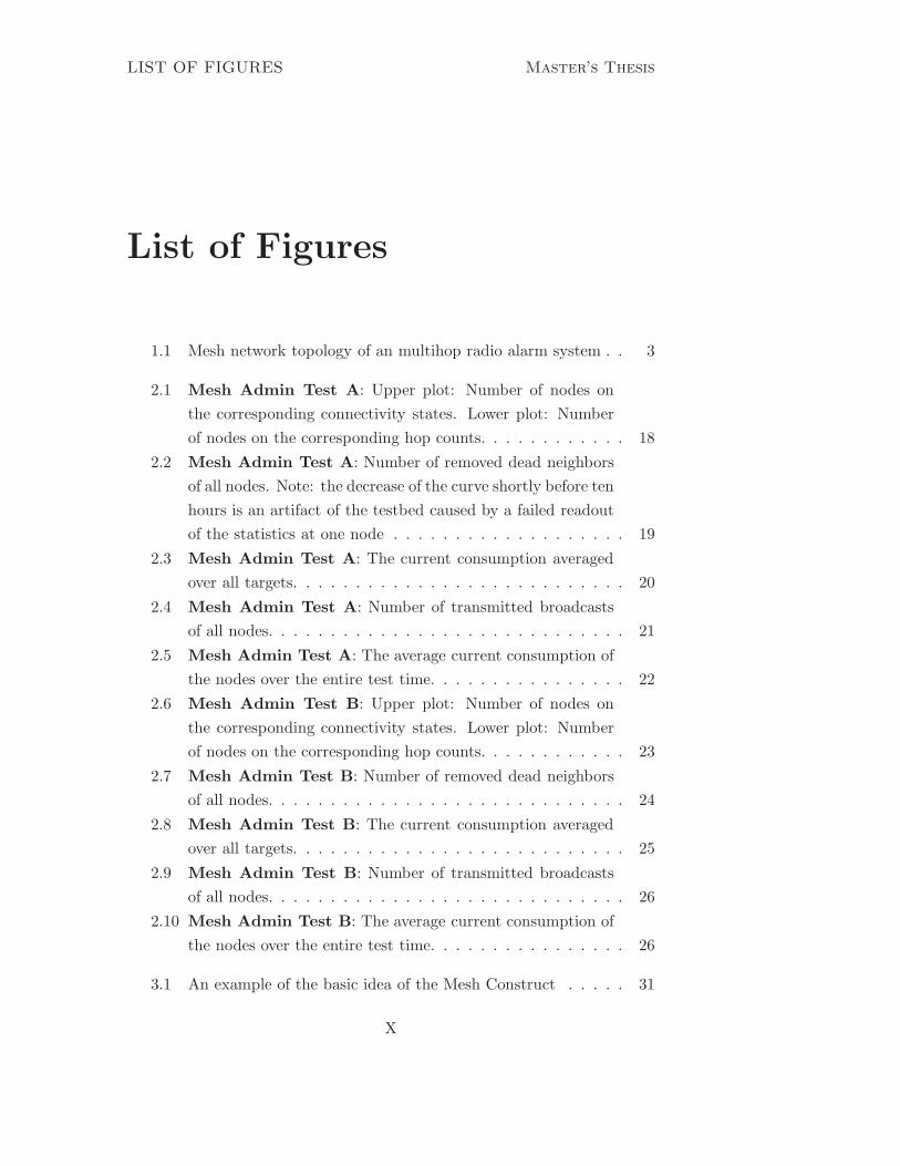
1.1 Mesh network topology of an multihop radio alarm system . . 3
2.1 Mesh Admin Test A: Upper plot: Number of nodes on
the corresponding connectivity states. Lower plot: Number
of nodes on the corresponding hop counts. . . . . . . . . . . . 18
2.2 Mesh Admin Test A: Number of removed dead neighbors
of all nodes. Note: the decrease of the curve shortly before ten
hours is an artifact of the testbed caused by a failed readout
of the statistics at one node . . . . . . . . . . . . . . . . . . . 19
2.3 Mesh Admin Test A: The current consumption averaged
over all targets. . . . . . . . . . . . . . . . . . . . . . . . . . . 20
2.4 Mesh Admin Test A: Number of transmitted broadcasts
of all nodes. . . . . . . . . . . . . . . . . . . . . . . . . . . . . 21
2.5 Mesh Admin Test A: The average current consumption of
the nodes over the entire test time. . . . . . . . . . . . . . . . 22
2.6 Mesh Admin Test B: Upper plot: Number of nodes on
the corresponding connectivity states. Lower plot: Number
of nodes on the corresponding hop counts. . . . . . . . . . . . 23
2.7 Mesh Admin Test B: Number of removed dead neighbors
of all nodes. . . . . . . . . . . . . . . . . . . . . . . . . . . . . 24
2.8 Mesh Admin Test B: The current consumption averaged
over all targets. . . . . . . . . . . . . . . . . . . . . . . . . . . 25
2.9 Mesh Admin Test B: Number of transmitted broadcasts
of all nodes. . . . . . . . . . . . . . . . . . . . . . . . . . . . . 26
2.10 Mesh Admin Test B: The average current consumption of
the nodes over the entire test time. . . . . . . . . . . . . . . . 26
3.1 An example of the basic idea of the Mesh Construct . . . . . 31
X

Master’s Thesis LIST OF FIGURES
3.2 Mesh Construct: Communication scheme of the gateway and
an arbitrary other discoverer . . . . . . . . . . . . . . . . . . 34
3.3 Neighborhood discovery of a single node: Communication
scheme of the discoverer and an arbitrary other node . . . . . 37
3.4 linear increasing txpower . . . . . . . . . . . . . . . . . . . . . 40
3.5 Scheme for transmitting a direct message . . . . . . . . . . . 54
3.6 Scheme for the duration of the timer t rx bcast . . . . . . . 56
3.7 Scheme for the duration of the timer t rx bcast rx . . . . . 57
4.1 Mesh Construct Test B: Timer t rx bcasts, discoverer
0002000D . . . . . . . . . . . . . . . . . . . . . . . . . . . . . 71
4.2 Mesh Construct Test B: Timer t rx bcast rx, discoverer
0002000D . . . . . . . . . . . . . . . . . . . . . . . . . . . . . 72
4.3 Mesh Construct Test B: Timer t rxack not, discoverer
0002000D . . . . . . . . . . . . . . . . . . . . . . . . . . . . . 72
4.4 Mesh Construct Test B: Timer t rxack not, discoverer
00020019 . . . . . . . . . . . . . . . . . . . . . . . . . . . . . 73
4.5 Mesh Construct Test B: Timer t rx ack start . . . . . . 74
4.6 Mesh Construct Test B: Timers t rx nhtbl and t rq nhtbl 76
4.7 Mesh Construct Test A: Upper plot: Number of nodes on
the corresponding connectivity states. Lower plot: Number
of nodes on the corresponding hop counts. . . . . . . . . . . . 78
4.8 Mesh Construct Test A: (non-operational phase) Upper
plot: Number of nodes on the corresponding connectivity
states. Lower plot: Number of nodes on the corresponding
hop counts. . . . . . . . . . . . . . . . . . . . . . . . . . . . . 79
4.9 Mesh Construct Test A: Number of removed dead neigh-
bors of all nodes. . . . . . . . . . . . . . . . . . . . . . . . . . 80
4.10 Mesh Construct Test A: The current consumption aver-
aged over all targets. . . . . . . . . . . . . . . . . . . . . . . . 80
4.11 Mesh Construct Test A: Number of transmitted broad-
casts of all nodes. . . . . . . . . . . . . . . . . . . . . . . . . . 81
4.12 Mesh Construct Test A: The average current consumption
of the nodes over the entire test time. . . . . . . . . . . . . . 82
4.13 Mesh Construct Test B: Upper plot: Number of nodes on
the corresponding connectivity states. Lower plot: Number
of nodes on the corresponding hop counts. . . . . . . . . . . . 83
XI
LIST OF FIGURES Master’s Thesis
4.14 Mesh Construct Test A: (non-operational phase) Upper
plot: Number of nodes on the corresponding connectivity
states. Lower plot: Number of nodes on the corresponding
hop counts. . . . . . . . . . . . . . . . . . . . . . . . . . . . . 84
4.15 Mesh Construct Test B: Number of removed dead neigh-
bors of all nodes. . . . . . . . . . . . . . . . . . . . . . . . . . 85
4.16 Mesh Construct Test B: The current consumption aver-
aged over all targets. . . . . . . . . . . . . . . . . . . . . . . . 86
4.17 Mesh Construct Test B: Number of transmitted broad-
casts of all nodes. . . . . . . . . . . . . . . . . . . . . . . . . . 87
4.18 Mesh Construct Test B: The average current consumption
of the nodes over the entire test time. . . . . . . . . . . . . . 87
4.19 Mesh Construct Test C: (non-operational phase) Upper
plot: Number of nodes on the corresponding connectivity
states. Lower plot: Number of nodes on the corresponding
hop counts. . . . . . . . . . . . . . . . . . . . . . . . . . . . . 89
4.20 Mesh Construct Test C: The current consumption aver-
aged over all targets. . . . . . . . . . . . . . . . . . . . . . . . 90
4.21 Mesh Construct Test C: The average current consumption
of the nodes during the Mesh Construct procedure. . . . . . . 91
XII

Master’s Thesis LIST OF TABLES
List of Tables
2.1 Mesh Admin variables for each entry of the neighbor table . . 15
2.2 Test parameters . . . . . . . . . . . . . . . . . . . . . . . . . . 16
2.3 Mesh Admin parameters . . . . . . . . . . . . . . . . . . . . . 17
3.1 Variables of the gateway . . . . . . . . . . . . . . . . . . . . . 43
3.2 Variables for each discoverer entry of the discvoerer table . . 43
3.3 Variables of a discoverer . . . . . . . . . . . . . . . . . . . . . 45
3.4 Variables for each node entry of the node table . . . . . . . . 45
3.5 Variables of a node . . . . . . . . . . . . . . . . . . . . . . . . 46
3.6 Variables for each neighbor entry of the neighbor table . . . . 47
3.7 Message fields of a broadcast . . . . . . . . . . . . . . . . . . . 47
3.8 Message fields of a broadcast received . . . . . . . . . . . . . . 48
3.9 Message fields of a notification . . . . . . . . . . . . . . . . . 49
3.10 Message fields of a ack notification . . . . . . . . . . . . . . . 49
3.11 Message fields of a neighbor table . . . . . . . . . . . . . . . . 50
3.12 Message fields of a ack start discovery . . . . . . . . . . . . . 51
3.13 Message fields of a ack completed . . . . . . . . . . . . . . . . 51
3.14 Message fields of a start discovery . . . . . . . . . . . . . . . 52
3.15 Message fields of a request neighbor table . . . . . . . . . . . . 52
3.16 Message fields of a completed . . . . . . . . . . . . . . . . . . 53
3.17 Parameters of Mesh Construct . . . . . . . . . . . . . . . . . 60
4.1 Test setup . . . . . . . . . . . . . . . . . . . . . . . . . . . . . 68
4.2 Parameters of the Mesh Construct tests . . . . . . . . . . . . 69
4.3 Energy consumption during the Mesh Construct procedure . 91
4.4 Comparison between the existing Solution (eS) and the Mesh
Construct (MC). (*: The maximal value after the network is
connected the first time until the test end is considered.) . . . 92
XIII

Introduction Chapter 1
Chapter 1
Introduction
A wireless sensor network (WSN) consists of a set of autonomous nodes,
each equipped with one or more sensors and a radio transceiver. The sensor
nodes can be deployed at distributed locations over an area in order to
jointly monitor various environmental conditions. The gained informations
from the sensors are processed and exchanged within the network by radio
communication.
Alarm systems require sensors to detect a possible danger, e.g. a thermal
or optical sensor for fire, or a motion sensor for intrusion. Detected dangers
are reported to a central station in order to raise alarm. For alarm systems,
often sensors are equipped with a radio transceiver and a pack of batteries
to save laborious and expensive wiring of detectors. A larger region than
the communication range of one single sensor can be monitored by deploying
several sensors in a WSN. The monitored area of a WSN alarm system can
additionally be increased with a mesh network topology. In a mesh network
alarms can be forwarded over multiple sensor nodes to the central station.
To ensure a reliable alarm reporting more than one multi hop routing path
from a sensor node to the central station is demanded in the network.
When a WSN alarm system has been installed, the individual sensor
nodes have no apriori knowledge about other existing nodes in the system.
Therefore, each node has to discover nodes in the vicinity to construct the
network topology. Discovered nodes are stored in a neighbor table. Through
the informations in the neighbor tables the multi hop communcation paths
from a sensor node to the central station can be deduced.
In this master thesis the algorithm Mesh Construct is presented. Mesh
Construct is a new procedure to perform a neighbor discovery and topology
1
Chapter 1 Introduction
construction with certain characteristics for an WSN alarm system. In the
special case of a wireless fire detection sensor network the mesh topology
requires at least two node-disjoint communication paths from a detector to
the central station to ensure a reliable alarm reporting also in case of a
detector failure.
In this report several parts have been removed due to confidentiality
reasons.
1.1 Setup
The underlying systems considered in this thesis is are radio alarm systems
based on a wireless sensor networks. However, the investigations in this
thesis are mostly focused on a wireless fire detection sensor network but
could also be generalized on an arbitrary radio alarm system.
1.1.1 Definitions
In the following some primary definitions of an radio alarm system are stated.
In Figure 1.1 the mesh topology of an exemplary radio alarm system is
shown.
• An alarm system consists of at least one gateway and one or more
detectors. The detectors are equipped with sensors which can detect
a danger event. In the case of a fire detection system the sensors are
thermal or optical and are able to detect a fire. If a danger emerges
and is detected the detectors report it to the gateway. The gateway
is connected with a central unit which processes the alarm messages.
The detectors and the gateway are also denoted as nodes.
• A radio alarm system is an alarm system where each node is equipped
with a radio transceiver.
• For the communcation within the network each node has a table of
nodes located in the vicinity, which are reachable by radio communi-
cation. The nodes listed in this table are called neighbors, the table is
denoted as neighbor table (Note: Not each node in the vicinity is nec-
essarily contained in the neighbor table!). Two nodes are neighboring,
if both are contained in the neighbor table of each other. The radio
connection between a node and one of its neighbors is denoted as link.
2

1.1 Setup Chapter 1
In Figure 1.1 for example node A and B are neighboring, but A and
C are not. The lines between the nodes symbolize the links.
Figure 1.1: Mesh network topology of an multihop radio alarm system
• A communication path is a sequence of consecutive links between two
nodes. For example in Figure 1.1 between the node M and the gateway
there are the communication paths (M, G, B, gateway) or (M, H, C,
gateway).
• A radio alarm system is denoted as linked if there exists a communi-
cation path between each pair of nodes. For example in Figure 1.1 the
alarm system without the node P is linked.
• A multihop radio alarm system is a radio alarm system in which the
3
Chapter 1 Introduction
gateway is not a neighbor of at least one detector. In Figure 1.1 a
multihop radio alarm system is shown.
In the following definitions the term ”system” is always used interchangeable
with the term ”linked multihop radio alarm system”.
• The hop count of a specific node denotes the minimal number of links,
which lie on the communication path from the node to the gateway
(Note: In the case of an asymmetric neighbor relation, i.e. a node
has added another node to its neighbor table but not vice versa, it is
crucial to start the communication path from the node and count the
links up to the gateway). In Figure 1.1 the gateway has hop count 0,
the nodes A, B, C, D, E, and F have hop count 1, the nodes G, H, I,
J, K, and L have hop count 2 and the nodes M, N, O, and P have hop
count 3.
• The neighbors of a specific node, that have a lower hop count as the
node itself, are called parents of this node.
• The neighbors of a specific node, that have the same hop count as the
node itself, are called peers of this node.
• The neighbors of a specific node, that have a higher hop count as the
node itself, are called children of this node.
For example in Figure 1.1 the node H has the parents C and D, the
peer G, and the child M.
• Two communication paths are denoted as independent if the commu-
nication paths between these two nodes contain no common nodes. In
Figure 1.1 the communication paths (M, G, B, gateway) and (M, H,
C, gateway) are independent.
• The number of connectivity paths of a detector denotes the number
of independent communication paths between this detector and the
gateway. The number of connectivity paths of the node M in Figure
1.1 is 2.
In a multihop radio alarm system, usually there is a number of connectiv-
ity paths, which is at least required in order to ensure reliable reporting of
alarms, e.g. in case of broken communication paths due to detector failures
4
1.1 Setup Chapter 1
or interference. The minimal required number of connectivity paths is a pa-
rameter of an alarm system (see Section 3.5) and in the following is denoted
as nb con paths min. To indicate the current number of connectivitiy paths
of a detector a connectivity state is introduced. The state of a detector can
be red, yellow, green, or green+.
• State red : The detector has no communication path to the gateway.
• State yellow : The detector has at least one communication path to
the gateway.
• State green: The detector has at least nb con paths min independent
communication paths to the gateway.
• State green+: This is an internal system state, which indicates that
the detector has at least nb con paths min independent communica-
tion paths to the gateway using only parents as next hops. Such a
detector may offer an additional independent communication path to
the gateway to peers with less than nb con paths min parents. The
connectivity state of a gateway is defined as green+.
In Figure 1.1 the parameter nb con paths min is set to 2. The connec-
tivity states of the nodes are indicated with the corresponding color,
whereas nodes with a green+ connectivity state have the color blue.
Additionally, a connectivity state for the entire network can be defined
analogously.
• The network connectivity state is green, if all detectors are at least
green.
• The network connectivity state is yellow, if each detector is at least
yellow.
• The network connectivity state is red, if at least one detector is red.
The alarm system shown in Figure 1.1 has a red network connectiv-
ity state. A network or a node is also denoted as connected, if the
connectivity state is at least green, and unconnected otherwise.
5
Chapter 1 Introduction
1.1.2 Multihop Wireless Fire Detection Sensor Network at
Siemens BT
Siemens BT Zug and the Swiss Federal Institute of Technology Zurich are
working together on a research project in the area of fire detection. The
objective of this project is to investigate the potentialities and capabilities
in the application of multihop wireless sensor networks for fire detection
systems. The multihop wireless fire detection sensor network investigated
at Siemens BT is an example of a radio alarm system.
The alarm system consists of at least one gateway and several fire de-
tectors, which together form a mesh network and communicate by radio on
the 433 MHz or 868 MHz industrial, scientific and medical (ISM) frequency
bands [1].
Each gateway is connected through a wire with an alarm-processing cen-
tral unit. The wired gateways have an additonal wireless interface, the
detectors are all wireless. On the one hand, ommitting wires eminently fa-
cilitates the installation of the fire detection system, but on the other hand,
requires the detectors to be powered by batteries. The battery supply limits
the lifetime of the detectors. Since the fire detection system is designed to
operate over several years, an energy consumption in the order of µW is
required.
To increase the system lifetime and reduce the maintenance costs of
changing batteries, the media access control is implemented through an low
power listening (LPL) protocol [2]. Since the radio transceiver is the com-
ponent of a node which consumes the most energy, with LPL the transceiver
is switched off the most time. The nodes with a switched off transceiver are
in an energy-efficient sleep mode and wake up only periodically for a short
carrier sense. If a signal is detected during the carrier sense, the node stays
awake and a message can possibly be received. Otherwise, the node returns
to the energy-efficient sleep mode. The nodes wake up independently of each
other with a periodic time interval t w. The wake up times of the indiviual
nodes are not synchronized to each other. In order to be sure to reach a
node a long preamble with the duration of one complete sleep interval t w
has to be prepended to the true message.
A further enhancement in terms of energy consumption is achieved with
the use of the WiseMAC [3] protocol. With WiseMAC, the wake up time
schedule is enclosed in the message header and is stored in the neighbor
6

1.2 Problem Description Chapter 1
table after each successful message reception. The knowledge of the wake
up times of neighbors allows a transmitting node to use an energy-efficient
short preamble and sending a message just before the destinated neighbor
wakes up. Only when the wake up time of a destination node is unknown a
long preamble has to be prepended to the message.
The longer the wake up period t w, the less energy is consumed for carrier
sense on average, but the more increased is the disbalance between messages
using a short and messages using a long preamble concerning energy con-
sumption.
For the communication between nodes of the network different message
types are used (see also Section 3.3). Two different direct messages are used
for the communication over the distance of one hop. A unicast message is
transmitted between a pair of nodes and uses a short preamble once the wake
up schedule of the destination is knwon. A broadcast message is transmitted
from a node to all reachable nodes in the vincinity. The broadcast message
uses always the long preamble in order to be sure that all nodes in the
vicinity wake up during the transmission and receive the message. Hence,
the transmission of a broadcast message causes a high energy consumption.
Two different message types for the communication over the distance of one
or more hops are transmitted. Dynamic source routing (DSR) messages are
used for the communication between a pair of nodes over possibly several
hops. Alarms are always transmitted from a detector to the gateway with
delay-aware robust forwarding (DWARF) messages [4].
The network initialization and topology control of the fire detection sys-
tem currently in use is accomplished by an individual protocol, which is
described and analyzed in Section 2.1.
1.2 Problem Description
1.2.1 Neighbor Discovery and Topology Construction
When a multihop wireless fire detection sensor network as described in Sec-
tion 1.1.2 shall be commissioned, all nodes have to be installed at distributed
locations over the entire area which has to be monitored. The gateway is
connected to the central unit and afterwards all detectors are sequentially
mounted and switched on. However, after the physical deployment the fire
detection system is not yet ready for operation because first, the network
7

Chapter 1 Introduction
topology has to be constructed in order to be able to forward and process
alarms.
When a node is powered on, the neighbor table is empty and no apriori
knowledge about other installed nodes in vicinity exists. Therefore, each
node has to perform a neighbor discovery in order to add nodes to the
neighbor table and construct the network topology. The network connec-
tivity state is green as soon as each installed detector is discovered and has
the minimum required number of connectivity paths to the gateway. From
then on, alarms can be forwarded reliably to the gateway and the operation
of the fire detection system can be started.
After the switch-on of the last detector, technicians which install the
system have to wait for the validation of the required green network connec-
tivity state and the approval of the proper operation of the alarm system.
Thus, the neighbor discovery and topology construction should be completed
in a reasonable time to ease the installation of the system.
During the operation in each node the topology control is performed
by the application described in 2.1. The application exchanges messages
between neighbors in a round robin way to monitor the network connec-
tivity state. When no more messages are received from a neighbor within
a certain period (e.g. due to collisions or a detector failure), the neighbor
appears to be dead and is removed from the neighbor table. Such a re-
moved neighbor is denoted as dead neighbor. Besides the topology control,
a link quality manager adapts the transmission power to save energy and
removes nodes from the neighbor table with poor link quality. If as a result
of removing a dead neighbor or a neighbor with poor link quality a node
loses the green/green+ connectivity state, new nodes have to be discovered
and added to the neighbor table. Certainly, nodes with a non-green connec-
tivity state are unwanted during operation because important connetivity
paths for alarm forwarding are missing. Additionaly, the discovering of new
neighbors requires to transmit broadcast messages which consume a lot of
energy.
Depending on the way which nodes are initially added to the neighbor
tables, the network topology eventually has to be adapted and is unstable
during the operation. In general, nodes which have a good link quality and
can improve the own connectivity state are prefered as neighbors. A lot of
energy wasting message retransmissions can be caused by a neighbor due to
8

1.2 Problem Description Chapter 1
a poor link quality. Additionally, more neighbors than are required to ensure
the green connectivity state are desired in the neighbor table to prevent a
connectivity state change due to a single neighbor removal. Therefore, the
initial choice of the neighbors is crucial for the construction of an energy-
efficient and stable network topology.
The Mesh Construct algorithm introduced in this thesis is implemented
as an additional protocol. The Mesh Construct shall perform neighbor dis-
covery and topology construction which is fast, energy-efficient and achieves
a connected and stable mesh network topology. After the Mesh Construct is
completed the operation is started and the existing application 2.1 accom-
plishes the topology control.
1.2.2 Requirements and Assumptions
Several requirements for the neighbor discovery and topology construction
of a fire alarm system are imposed by Siemens BT as well as by regulatory
norms.
• The fire detection system shall ensure the capability of alarming also
in case of a detector failure. Hence, each detector must have at least
more than one independent communication path to the gateway. In
particular, the paramteter nb con paths min of the minimal number
of required connectivity paths is set to 2. The neighbor discovery
and topology construction has to be completed in a green network
connectivity state. Exception is a system consisting of one gateway
and only one detector [5, 4.3].
• The mesh network of the fire detection system has maximal three hops.
• The neighbor discovery and topology construction procedure has to
be completed in a finite duration, at longest one hour after switching
on the last installed node. Nevertheless, the duration of the commis-
sioning shall be as short as possible to provide an easy installation of
the fire alarm system.
• The memory resources of a detector are limited and are insufficient
to store the informations of the entire network. Thus, the own con-
nectivity state has to be identified by local available informations and
informations from the direct, immediate neighborhood.
9

Chapter 1 Introduction
• The Mesh Construct procedure for neighbor discovery and topology
construction shall be implemented as new protocol in the existing soft-
ware.
In the scope of this thesis several assumptions are made, which are stated
in the following:
• Only one gateway is contained in the wireless fire detection sensor
network.
• When a node is installed and switched on, no topology and neighbor-
hood information about other network nodes is known a priori in the
node.
1.2.3 Quality Metrics and Objectives
The neighbor discovery and topology construction is a multi objective opt-
miziation problem. In this section the various objectives of the new proce-
dure for the neighbor discovery and topology construction are stated. Ad-
ditionally, metrics to assess the quality of the procedure are defined.
Duration
An important quality is the duration which is required to achieve a green
/green+ network connectivity state. The objective is that the technicians
installing the alarm system can approve the required network connectivity
state as fast as possible. Therefore, the following metric is defined to assess
the procedure quality concerning the duration.
• The duration t connected from the last switch on of a node until all
installed nodes have a green/green+ connectivity state is a metric for
the tempo of the procedure. The objective is to achieve a t connected
as short as possible.
Connectivity
The essential property a procedure for neighbor discovery and topology con-
struction must feature, is to initialize the alarm system for the proper oper-
ation. The requirement for the start of the operation is determined by the
connectivity state. The objective of the procedure in terms of connectivity is
10
1.2 Problem Description Chapter 1
that, all installed nodes are discovered and achieve the required connectivity
state, which is at least green or green+. This ensures the reliable forwarding
of raised alarms to the central unit during the operation.
The following two metrics are defined to determine if all installed nodes
are discovered on the one side and on the other side have the required
connectivity state.
• The number of nodes with a red connectivity state nb red nds is a
metric for the discovering state of the network. The lower nb red nds,
the better discovered are the installed nodes. The objetive is to achieve
nb red nds = 0.
• The number of nodes with a red or yellow connectivity state nb red-
yellow nds is a metric for the connectivity of the network. The
lower nb redyellow nds, the more nodes have the required number
of connectivity paths to the gateway. The objective is to achieve
nb redyellow nds = 0.
Stability
Besides the connectivity and the duration of the procedure for neighbor
discovery and topology construction, it is essential that the network remains
connected during operation. The removal of dead appearing neighbors by
the topology control algorithm can cause a change of the connectivity state
to yellow or red. Subsequently, nodes start to broadcast and to discover
new neighbors. For that reason, the network topology can change over
time. Certainly, this is unwanted since the adaption of the network topology
consumes additional energy to get connected again. Hence, the objective
of a neighbor discovery and topology construction is to provide a network
topology which is stable during the operation with enabled topology control
application. The following two metrics are defined to assess the procedure
quality concerning the stability.
• The number of removed dead neighbors nb rem dead nhs is a metric
for the stability. The lower the nb rem dead nhs is, the more stable is
the network topology. The objective is to achieve nb rem dead nhs =
0.
• Additionally, the change of the node connectivity states over time is a
metric for the stability (Note: Although this is a metric to assess the
11

Chapter 1 Introduction
procedure in a rather qualitative way, it allows to make very meaning-
ful statements for individual test results. To analyze a large number
of tests a metric representing a numeric value should be defined). The
objective is to achieve connectivity states which are constant over time.
The number of neighbors removed by the link quality manager is not
tracked in the statistic tool used for the tests in Section 2.1.2 and Chapter
4. Therefore, the number of neighbors removed by the link quality manager
is excluded from the quality metrics but is sometimes mentioned in the
stability evaluation.
Energy Consumption
The energy consumption is also an essential aspect of a neighbor discovery
and topology construction procedure. Since the detectors are powered by
batteries, the energy budget and therefore the lifetime of the alarm system
is limited. The objective is to minimize the energy consumption to increase
the system lifetime and reduce the maintenance costs. The following two
metrics are defined to assess the procedure quality concerning the energy
consumption.
• The total current i total averaged over time and the number of nodes
is a metric for the energy consumption.
• Additionally, the number of transmitted broadcasts nb tx bcasts is
a metric for the energy consumption. The transmission of broadcast
messages contributes substantially to the energy consumption.
The gateway is excluded from the energy considerations since it is wired
and not powered by batteries.
1.3 Chapters Overview
The thesis is structured in 5 chapters. In Chapter 2 the existing solution
for the network initialization and topology control and related work is in-
vestigated. In Chapter 3 the conceptual design of the new procedure for
neighbor discovery and topology construction is presented. Moreover, a few
implementation details are indicated. In Chapter 4 the new procedure is
tested and evaluated. In addition, the new procedure is compared to the
12

1.3 Chapters Overview Chapter 1
existing solution described in Chapter 2 in terms of the metrics defined in
Section 1.2.3. In Chapter 5 the obtained conclusions of the evaluation in
Chapter 4 are stated and an outlook on possible future work is given.
13

Chapter 2 Background and Related Work
Chapter 2
Background and Related
Work
In the first section of this chapter the existing solution for the network
initialization and the topology control of the fire detection system presented
in section 1.1.2 is explained, tested, and evaluated.
In the second section related work in the area of neighbor discovery and
topology construction as well as link quality estimation is outlined.
2.1 Analysis of Existing Solution - Mesh Admin
Mesh Admin is the name of the existing protocol for neighbor discovery and
topology control in the wireless fire detection sensor network of Siemens BT.
The Mesh Admin is a random procedure, where each node after be-
ing switched on autonomously discovers neighbors in the vicinity through
the transmission of HELLO-broadcast messages. Other nodes receiving a
HELLO-broadcast message add the source to the neighbor table and period-
ically transmit direct hello-unicast messages to all its neighbors in a round
robin way. Among other things, each message contains information about
the source node, e.g. the hop count and connectivity state. Successively,
information about neighboring nodes is collected through this message ex-
change and updated in the neighbor table. The table has up to eight entries
for discovered and added neighbors. For each listed neighbor the following
informations are stored as fields in the neighbor table:
Each node is able to determine its own hop count and connectivity state
14

2.1 Analysis of Existing Solution - Mesh Admin Chapter 2
Neighbor table Neighbor table variable description
nd add Node address of the neighbor
hop count Hop count
con state Connectivity state
check timer flag Indicates if a message from the neighbor is
received within the last check timer period
Table 2.1: Mesh Admin variables for each entry of the neighbor table
through the informations provided in the neighbor table (see also Algorithm
1). The nodes communicate periodically with its neighbors and exchange
informations of the neighbor table such that the nodes can update their own
connectivity state. If the own connectivity state is insufficient, periodically
further broadcasts are transmitted in order to discover new neighbors which
can lend the desired connectivity state. Changes in the topology are only
propagated through the hello-unicasts. Adjustements can take some time
when several hops need to be adjusted. By this means, the whole network
topology is constructed and maintained. In a node the protocol is started
with the swith-on and runs infinitely long.
2.1.1 Connectivity State Update
A procedure will be presented, which allows to determine the connectivity
state of a detector only with local available information in the neighbor table,
that is, the hop count and the connectivity state of neighboring nodes. First,
the own hop count is identified by searching for the minimal hop count in
the neighbor table, then the own hop count is one higher. Through the own
hop count each neighbor can be identified either as parent, peer, or child.
In the following the procedure to determine the own connectivity state is
indicated in Algorithm 1.
Note: The Algorithm 1 has only available local network information
from the neighbor table. The procedure ensures that with a resulting
green/green+ connectivity state there are at least nb con paths min con-
nectivity paths, with a resulting yellow connectivity state there is at least
one connectivity path. The reverse is not necessarily true. For example
for node I in Figure 1.1 the Algorithm 1 returns a yellow connectivity state
although there are two connectivity paths in the network.
15

Chapter 2 Background and Related Work
Important neighbors, which causes the node to achieve or maintain a
green/green+ connectivity state, are locked to avoid beeing deleted if a
neighbor should be added to a full neighbor table. In the following the
procedure to lock important neighbors is indicated in Algorithm 2. The
detailed communcation procedure among nodes is described in the next
section.
2.1.2 Testing and Evaluation
The performance of the Mesh Admin algorithm is assessed through longterm
tests on an experimental setup. The used testbed is described in Appendix
A. Through a statistic tool and logs on the nodes various informations for
an evaluation are collected during the test runtime. The number of nodes
nb nds of the testbed is 32. The test setup consists of one gateway and 31
detectors. At the beginning of the test first, the gateway is switched on
and afterwards sequentially all detectors in a random order. Before a node
is enabled, a time delay is inserted to simulate the installation time. The
time delay between the startup of two succeding nodes is uniform random
distributed in the interval [t min, t max]. The time delay due to the installa-
tion is set to be between one and five minutes. The test runtime t test starts
after the last switch-on and is set to twelve hours. The test parameters are
listed in Table 2.2.
Test Parameters Value
nb nds 32
t test 43200 s
t min 60 s
t max 300 s
Table 2.2: Test parameters
The set values of the Mesh Admin parameters are listed in Table 2.3.
Many longterm Mesh Admin tests have been run on the testbed. How-
ever, the number of performed tests does not claim to be statistical relevant
and therefore in the following only two typical test examples thereof are
shown and evaluated.
Mesh Admin Test A
16

2.1 Analysis of Existing Solution - Mesh Admin Chapter 2
Algorithm 1 Connectivity State Update1: if hop count == 1 then
2: if number of peers ≥ nb con paths min then
3: own con state = green+
4: else
5: own con state = yellow
6: end if
7: end if
8:
9: if hop count > 1 then
10: if number of green/green+ parents ≥ nb con paths min - 1 then
11: own con state = green+
12: else
13: if number of green/green+ parents and green+ peers ≥ nb con paths min then
14: own con state = green
15: else
16: if number of parents > 0 then
17: own con state = yellow
18: else
19: own con state = red
20: end if
21: end if
22: end if
23: end if
Algorithm 2 Lock Neighbors1: if hop count == 1 then
2: lock the gateway and one arbitrary peer
3: end if
4:
5: if hop count > 1 then
6: lock green/green+ parents, at most nb con paths min
7: lock green+ peers at most nb con paths min neighbors in total
8: lock other parents, until a total number of locked neighbors is nb con paths min neighbors
in total
9: if no neighbors have been locked so far, lock at leat 1 parent.
10: end if
Mesh Admin Parameters Value
t w 1.5 s
nb con paths min 2
hello timer 240 s
check timer 16 · 240 s = 3840 s
happpy timer 20 · 240 s = 4800 s
Table 2.3: Mesh Admin parameters
17

Chapter 2 Background and Related Work
0 2 4 6 8 10 12hours
0
5
10
15
20
25
30
35
40
num
ber
of
nodes
on c
onnect
ivit
y s
tate
green+greenyellow
redlast switch-onconnected
0 2 4 6 8 10 12hours
0
5
10
15
20
25
30
35
40
num
ber
of
nodes
wit
h h
op c
ount
hc 0hc 1hc 2hc 3hc > 3last switch-onconnected
Figure 2.1: Mesh Admin Test A: Upper plot: Number of nodes on the
corresponding connectivity states. Lower plot: Number of nodes on the
corresponding hop counts.
18
2.1 Analysis of Existing Solution - Mesh Admin Chapter 2
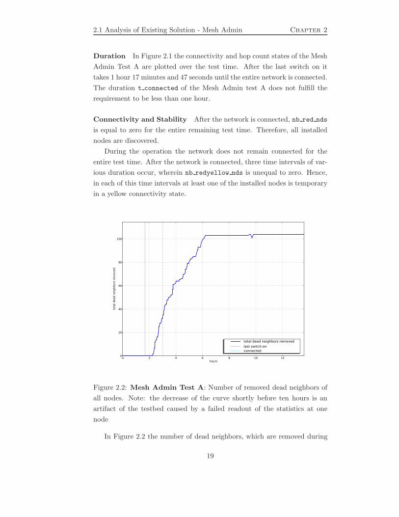
Duration In Figure 2.1 the connectivity and hop count states of the Mesh
Admin Test A are plotted over the test time. After the last switch on it
takes 1 hour 17 minutes and 47 seconds until the entire network is connected.
The duration t connected of the Mesh Admin test A does not fulfill the
requirement to be less than one hour.
Connectivity and Stability After the network is connected, nb red nds
is equal to zero for the entire remaining test time. Therefore, all installed
nodes are discovered.
During the operation the network does not remain connected for the
entire test time. After the network is connected, three time intervals of var-
ious duration occur, wherein nb redyellow nds is unequal to zero. Hence,
in each of this time intervals at least one of the installed nodes is temporary
in a yellow connectivity state.
0 2 4 6 8 10 12hours
0
20
40
60
80
100
tota
l dead n
eig
hbors
rem
oved
total dead neighbors removed
last switch-onconnected
Figure 2.2: Mesh Admin Test A: Number of removed dead neighbors of
all nodes. Note: the decrease of the curve shortly before ten hours is an
artifact of the testbed caused by a failed readout of the statistics at one
node
In Figure 2.2 the number of dead neighbors, which are removed during
19

Chapter 2 Background and Related Work
the test, is plotted over the test time. In total nb rem dead nhs = 104
dead neighbors are removed during the test, all of them in the first six
hours. Thus, the two time intervals with yellow network connectivity states
towards the end of the test are caused by neighbor removals of the link
quality manager. A causality between the removal of dead neighbors in the
first six hours and the corresponding unstable time course of the connectivity
states in Figure 2.1 can be recognized. Between the neighbor removals the
network reaches an intermediate, almost stable and connected state.
0 2 4 6 8 10 12 14time [h]
0
50
100
150
200
250
300
350
400
450
curr
ent
[uA
]
average current consumption of all targets:
I_sleep
I_carriersense
I_overhear
I_rx
I_tx
last switch-onconnected
Figure 2.3: Mesh Admin Test A: The current consumption averaged over
all targets.
Energy Consumption In Figure 2.3 the current consumtpion averaged
over all targets is plotted over the test time. The total consumed current
of the Mesh Admin Test A is divided into the five contributions I sleep,
I carriersense, I overhear, I rx, and I tx. I sleep is the current con-
sumed in the energy-efficient sleep state. I carriersense is the current
required for the periodic wake up and carrier sense. I overhear is the cur-
rent consumed for receiving messages which originally are transmitted to a
different destination. I rx, and I tx are the currents consumed for receiving
and transmitting messages.
Until the network is connected the most energy is consumed, in particu-
lar due to the transmissions of the energy expensive broadcasts. The number
of transmitted broadcasts is plotted in Figure 2.4 over the testtime. The
20

2.1 Analysis of Existing Solution - Mesh Admin Chapter 2
total number of transmitted broadcasts nb tx bcasts during the test is 37.
Thus, several nodes had to transmit more than one broadcast. By compar-
0 2 4 6 8 10 12hours
0
5
10
15
20
25
30
35
40
tota
l tr
ansm
itte
d b
roadca
sts
total transmitted broadcastslast switch-onconnected
Figure 2.4: Mesh Admin Test A: Number of transmitted broadcasts of
all nodes.
ing the time course of the current consumption with the time course of the
connectivity states in Figure 2.1, a relation between the energy consump-
tion and the stability of the connecivity states can be observed. The energy
consumption in the network is higher in time intervals of unstable connec-
tivity. In Figure 2.5 the current consumption of each individual detector
averaged over the entire test time is shown. Again, the current consump-
tion is divided into its five contributions. Although there are some nodes
with a higher total current, overall the current consumption of the nodes is
rather balanced. The total current consumption averaged over the time and
number of nodes i total is 144.090 µA.
Mesh Admin Test B
Duration In Figure 2.6 the connectivity and hop count states of the Mesh
Admin Test B are plotted over the test time. In contrast to the Mesh Admin
21

Chapter 2 Background and Related Work
00020044
00020005
00020014
00020022
0002003b
0002001d
0002000c
00020021
00020003
00020015
00020008
00020013
0002000e
00020018
0002001e
0002001a
0002000b
0002000d
0002000f
00020001
0002000a
00020046
00020020
00020012
00020010
00020017
00020043
00020009
00020045
0002001f
000200190
100
200
300
400
500cu
rrent
[uA
]
average current consumption of the targets
I_sleepI_carriersenseI_overhearI_rxI_tx
Figure 2.5: Mesh Admin Test A: The average current consumption of
the nodes over the entire test time.
Test A, after the last switch on it takes only 17 minutes and 22 seconds until
the entire network is connected. The duration t connected of the Mesh
Admin test B clearly fulfills the requirement to be less than one hour.
Connectivity and Stability In Figure 2.6 the connectivity and hop
count states of the Mesh Admin Test B are plotted over the test time.
After the network is connected, nb red nds is equal to zero for the entire
remaining test time. Therefore, all installed nodes are discovered.
Like in the Mesh Admin Test A, during the operation the network does
not remain connected for the entire test time. After the network is con-
nected, five time intervals of various duration occur, wherein nb redyellow-
nds = 1, 2. Hence, each time one or two of the installed nodes are tempo-
rary in a yellow connectivity state.
In Figure 2.7 the number of dead neighbors, which are removed during
the operation, is plotted over the test time. In total nb rem dead nhs = 89
dead neighbors are removed during the test, all of them in the first six
hours. Thus, the last three time intervals with yellow network connectivity
states are caused by neighbor removals of the link quality manager. A
causality between the removal of dead neighbors in the first six hours and the
corresponding unstable time course of the connectivity states in Figure 2.6
22

2.1 Analysis of Existing Solution - Mesh Admin Chapter 2
0 2 4 6 8 10 12hours
0
5
10
15
20
25
30
35
40
num
ber
of
nodes
on c
onnect
ivit
y s
tate
green+greenyellow
redlast switch-onconnected
0 2 4 6 8 10 12hours
0
5
10
15
20
25
num
ber
of
nodes
wit
h h
op c
ount
hc 0hc 1hc 2hc 3hc > 3last switch-onconnected
Figure 2.6: Mesh Admin Test B: Upper plot: Number of nodes on the
corresponding connectivity states. Lower plot: Number of nodes on the
corresponding hop counts.
23

Chapter 2 Background and Related Work
0 2 4 6 8 10 12hours
0
20
40
60
80
tota
l dead n
eig
hbors
rem
oved
total dead neighbors removed
last switch-onconnected
Figure 2.7: Mesh Admin Test B: Number of removed dead neighbors of
all nodes.
24

2.1 Analysis of Existing Solution - Mesh Admin Chapter 2
can be recognized. However, not each neighbor removal necessarily causes
a connectivity state change, e.g. when a child is removed from the neighbor
table. Therefore, in contrast to the Mesh Admin Test A the last dead
neighbor removals did not affect the connectivity state of the nodes. Between
the neighbor removals the network reaches short, intermediate, almost stable
and connected states.
0 2 4 6 8 10 12 14time [h]
0
100
200
300
400
500
600
curr
ent
[uA
]
average current consumption of all targets:
I_sleep
I_carriersense
I_overhear
I_rx
I_tx
last switch-onconnected
Figure 2.8: Mesh Admin Test B: The current consumption averaged over
all targets.
Energy Consumption In Figure 2.8 the current consumtpion averaged
over all targets is plotted over the test time. The total consumed current of
the Mesh Admin Test B is again divided into its five contributions.
Analogous to the Mesh Admin Test A, the most energy is consumed by
the transmissions of the energy expensive broadcasts during the neighbor
discovery and topology control. The number of transmitted broadcasts is
plotted in Figure 2.9 over the testtime. The total number of transmitted
broadcasts nb tx bcasts during the test is 36. Thus, several nodes had to
transmit more than one broadcast.
By comparing the time course of the current consumption with the time
course of the connectivity states in Figure 2.6, again a higher energy con-
sumption during time intervals of unstable connectivity can be observed.
In Figure 2.10 the current consumption of each individual detector av-
eraged over the entire test time is shown. In contrast to the Mesh Admin
25

Chapter 2 Background and Related Work
0 2 4 6 8 10 12hours
0
5
10
15
20
25
30
35
tota
l tr
ansm
itte
d b
roadca
sts
total transmitted broadcastslast switch-onconnected
Figure 2.9: Mesh Admin Test B: Number of transmitted broadcasts of
all nodes.
0002000c
00020005
0002000b
00020001
00020008
0002001a
00020020
00020018
0002000a
00020022
0002001f
00020003
00020013
00020009
00020019
0002001e
00020021
00020043
00020045
00020012
0002001d
00020015
00020010
0002000e
00020017
00020014
00020044
0002000f
00020046
0002003b
0002000d0
100
200
300
400
500
curr
ent
[uA
]
average current consumption of the targets
I_sleepI_carriersenseI_overhearI_rxI_tx
Figure 2.10: Mesh Admin Test B: The average current consumption of
the nodes over the entire test time.
26
2.2 Related Work Chapter 2
Test A, there are two nodes with a total current consumption which is about
three times higher than the one of the other nodes. The operation of these
detectors is eminently endangered by an early depletion of the batteries.
The total current consumption averaged over the time and number of nodes
i total is 123.536 µA.
Conclusions
The individual Mesh Admin test results do not reveal a homogenous be-
haviour. The randomness of the Mesh Admin procedure is clearly recog-
nizable in the plots. For example the duration t connected is eminently
variable. Additionally, there is no finite deterministic upper bound for the
duration of the neighbor discovery and topology control.
The main observation of the longterm tests is the unstable time course
of the connectivity and hop count states. As registered in the last sections
the removal of neighbors, which ensure the required connectivity state, is
responsible for the instability. The removals can consist of both, dead neigh-
bors or neighbors with a poor link quality.
Moreover, the instability of the network connectivity state causes the
unconnected nodes to transmit further messages to discover new neighbors,
in particular energy expensive broadcasts. By this, the energy consumption
on the battery powered detectors is additionally increased.
Therefore, the initial choice of neighbors is crucial for the stability and
the energy consumption during the future operation of the alarm system.
2.2 Related Work
In this section an overview of previous work in the area of neighbor discovery
and topology construction as well as link quality estimation is given.
2.2.1 NoSE: Neighbor Search and Estimation
Meier et al. in [6] and [7] propose with NoSE a time and energy-efficient
initialization of a WSN. A wake up call functionality is included for switching
the network from an energy-efficient sleep state through a neighbor discovery
to an operational state where the topology can be set up. The wake up call
can be flooded into the network by an external trigger and initiates with
a timer mechanism the simultaneous start of a discovery phase with finite
27

Chapter 2 Background and Related Work
duration. During the discovery all nodes transmit a predefined number of
discovery packets. Moreover, the nodes track the number of received packets
and the corresponding RSSI to assess the link quality providing a basis for
the topology set up. Energy is saved by the simultaneous discovery start
and the appropiate adjusting of the wake up period of the MAC protocol
for the different operational states.
2.2.2 Birthday Protocols
A popular approach for initializing WSNs is proposed in the Birthday Pro-
tocols [8] by McGlynn and Borbash. The neighbor discovery is started by an
external trigger. The time is slotted and each node decides independently
and randomly at the beginning of each timeslot for a sleep, listen, or trans-
mit state. A neighbor is added when a node in the listen state receives a
broadcast discovery message from another node in the transmit state. The
discovery period has a finite duration after which neighbors have either been
discovered or never will be.
The birthay protocols provide no information about the link quality of
discovered neighbors. The size of the neighbor table is not limited, which is
not given in the implementation on a practical setup. Additionally, a MAC
protocol with synchronized wake ups is required to enable the slotted time.
2.2.3 XTC
Wattenhofer and Zollinger proposed XTC [9], a practical topology control
algorithm for ad-hoc networks. The algorithm has three main contributions.
The algorithm choses neighbors solely based on local information by com-
municating only twice with nodes, works for general network graphs, and
does not require node position information. The algorithm orders neighbors
according to the link qualities, exchanges the neighbor orders and selects
topology control neighbors. If the algorithm is applied to a unit disk graph,
the resulting network topology has a bounded degree of at most 6, i.e. the
size of the neighbor table is limited to 6 neighbors.
Since the memory on sensor nodes usually is very scarce, the limited
neighbor table property of the topology control algorithm is interesting.
However, the unit disk graph assumes uniform radio propagation as in the
vacuum, which is not practical.
28

2.2 Related Work Chapter 2
2.2.4 A Simple Algorithm
Angelosanto et al. in [10] present a simple algorithm for neighbor discovery
in wireless networks. The algorithm assumes slotted time and a neighbor
discovery of limited duration. Nodes are indentified by a signature and ran-
domly either transmit or receive during a time slot under constant probabili-
ties. The neighbor discovery is solved by adding a neighbor if the correlation
between the receive signal and the signatur of the node exceeds an discovery
threshold. Collisions are avoided by using orthogonal signatures.
Analogously to the Birthday Protocols, the simple algorithm requires a
MAC protocol supporting synchronized wake ups. Additionally, the nodes
have to keep an apriori known list with all signatures of the network.
2.2.5 Link Quality Estimation
Meier et al. in [11] showed that the deployment of a typical multihop WSN
based on low power radios results in a network with a large percentage of
very poor link characteristics. A pattern based link estimation scheme is
presented which allows to rate the link quality in an energy-efficient way
during the initialization phase in order to construct optimal neighbor tables
from the beginning.
Srinivasan and Levis in [12] showed that for new transceivers the RSSI
above the sensitivity threshold is a promising link quality indicator. A RSSI
above the sensitivity threshold results in a packet reception rate (PRR) of
at least 85%, whereas around the sensitivity threshold the RSSI does not
have a good correlation with the PRR.
29
Chapter 3 Conceptual Design
Chapter 3
Conceptual Design
In this chapter the conceptual design of the Mesh Construct is presented.
The first section outlines the basic idea of the Mesh Construct. In the
following sections the details of the procedure concerning the different node
functions, messages, timers, and parameters are explained in more depth.
In the subsequent section pseudocodes of the three main components of the
procedure are indicated. In the last section the maximal duration of the
Mesh Construct procedure is theoretically derived.
In this chapter various variables and fields, messages, and parameters
are introduced. For a better visualization variable and field names are
written in typewriter font, message names are written as emphasized text,
and parameter names are typeset as sans serif.
3.1 Basic Idea of Mesh Construct
The Mesh Construct algorithm is a deterministic procedure to construct
a mesh network topology for a wireless fire detection sensor network. The
Mesh Construct differs in several essential aspects from the existing solution
(see Section 2.1). The existing solution is a random procedure with an
infinite duration, which is running completely autonomously on each node.
In contrast to that, the Mesh Construct is a deterministic procedure which
is finished after a finite duration. Additionally, the procedure is no longer
running completely autonomously on each node but is controlled centrally
by the gateway.
In the Mesh Construct algorithm there are three different functions a
network node can fullfil, either gateway, discoverer, or, just a neighboring
30
3.1 Basic Idea of Mesh Construct Chapter 3
Figure 3.1: An example of the basic idea of the Mesh Construct
31
Chapter 3 Conceptual Design
node. The gateway functionality is contained only in one single node in
the whole network. The discoverer and node functionality is contained in
each node, also in the gateway. The node with the gateway functionality
acts like a choirmaster who conducts the construction of the mesh network
and arranges the time periods where the discoverers are allowed to discover
potential neighbors. A node in the discoverer function performs a neigh-
borhood discovery in order to find other nodes in mutual radio range. The
discoverer chooses the most suitable nodes for the purpose of the network
as neighbors and transmits its choice in form of a neighbor table message to
the gateway. The gateway successiveley stores and maintains the received
neighbor tables to gain information about the whole mesh network topology.
The functionality of a neighboring node denotes a node interacting with a
discoverer. The three different node functions are described in Section 3.2.
The different messages used for the communication between the nodes are
described in Section 3.3.
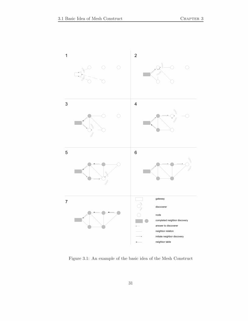
An easy example of the Mesh Construct procedure for a small num-
ber of nodes is illustrated in Figure 3.1. The underlying idea of the Mesh
Construct is to start from the network center at the gateway and construct
the mesh network through neighborhood discoveries by proceeding outwards
hop by hop. First, the gateway self performs a neighborhood discovery as
a discoverer to find neighbors with hop count 1 (number 1 in Figure 3.1).
Not all discovered nodes are necessarily chosen as neighbors. Next, further
neighborhood discoveries are sequentially initiated by the gateway on each
node with hop count 1 (number 2 and 3 in Figure 3.1). After the comple-
tion of these neighborhood discoveries a network consisting of nodes with
hop count 1 and 2 is constructed. Through the received neighbor tables of
nodes with hop count 1 the gateway has obtained informations about the
children of the nodes with hop count 1, which are nodes with hop count
2. In this manner the gateway succesively continues to sequentially arrange
neighborhood discoveries on the next hop to find new nodes and construct
the mesh network (number 4, 5 and 6 in Figure 3.1). The Mesh Construct
algorithm stops if the neighbor tables of all installed nodes are received or
the maximal number of allowed hops is attained (number 7 in Figure 3.1).
After the Mesh Construct is completed the installed nodes are part of a
constructed mesh network and the primary scheduled operation (e.g. fire
detection) with network topology control can be started.
32

3.1 Basic Idea of Mesh Construct Chapter 3
The whole Mesh Construct procedure is described more detailed in Sec-
tion 3.1.1. The neighborhood discovery is an component of the Mesh Con-
struct algorithm and is described in Section 3.1.2. The choice of the neighbor
nodes is a component of the neighborhood discovery algorithm and is de-
scribed in Section 3.1.3.
3.1.1 Mesh Construct
The Mesh Construct is the basic procedure and can be started by a trigger
mechanism at the gateway after the last detector of a wireless fire detection
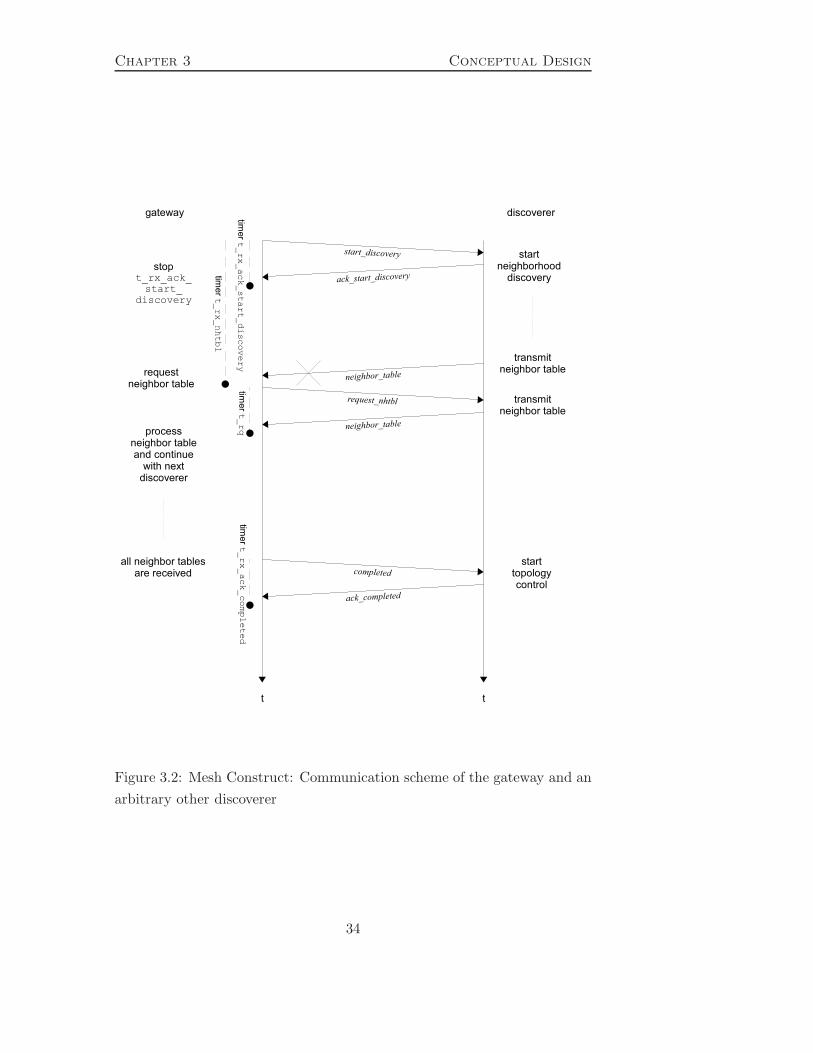
sensor network is physically installed. The communication scheme of the
gateway and an arbitrary discoverer during the Mesh Construct is shown
in the Figure 3.2. The Mesh Construct procedure is also described in the
pseudocode of algorithm 3 in Section 3.6. All message types exchanged
between the gateway and the discoverer are described in Section 3.3.
Due to the fact that the transmission medium is wireless, it can always
be assumed that a message is not received at the destination because of a
collision or any type of interference. Therefore, the whole procedure must
be able to cope with missing messages at any time. Timers and retry mecha-
nisms with thresholds for the number of retries are introduced to prevent the
algorithm from stopping. The different applied timers are described more
detailed in Section 3.4.
Once the Mesh Construct is started by the trigger, the gateway per-
forms a complete neighborhood discovery. Afterwards, the gateway stores
its added neighbors with hop count 1 as future discoverers in a discoverer
table discoverer tbl. All variables and fields of the Mesh Construct pro-
cedure are defined in Section 3.2. In the following the gateway sequentially
initiates the procedure shown in the Figure 3.2 on each discoverer in the
discoverer table in order to allow temporal non-overlapping neighborhood
discoveries. The hop count of the discoverer performing the current neigh-
borhood discovery is denoted as the Mesh Construct state mc state.
The gateway transmits a start discovery message to the first discoverer in
discoverer tbl and starts the two timers t rx ack start and t rx nhtbl
simultaneously. As a reaction on receiving a start discovery the first discov-
erer starts the neighborhood discovery procedure and transmits an ack start-
discovery back to the gateway. If an ack start discovery is received at the
gateway, the timer t rx ack start is stopped. When t rx ack start ex-
33
Chapter 3 Conceptual Design
Figure 3.2: Mesh Construct: Communication scheme of the gateway and an
arbitrary other discoverer
34

3.1 Basic Idea of Mesh Construct Chapter 3
pires and the number of retries rtr start has not already exceeded the
threshold rtr start max, another start discovery is transmitted and the two
timers are restarted. Otherwise the start of the neighborhood discovery
failed, and the procedure continues with the next discoverer.
As soon as a neighborhood discovery is completed, the discoverer node
transmits its neighbor tbl in a neighbor table message to the gateway. If
the timer t rx nhtbl at the gateway expires without having received the
expected neighbor table and the number of retries rtr request has not ex-
ceeded the threshold rtr request max, then a request nhtbl message is trans-
mitted to the discoverer. When the timer t rx nhtbl expires, it implies that
the timer t rx ack start has been stopped and an ack start is already re-
ceived. Therefore, the neighborhood discovery should already be completed
and an other, shorter timer t rq is started for the requesting of the neighbor
table. When the timer t rq expires another request nhtbl is transmitted if
the retries have not exceeded the threshold rtr request max, otherwise the
transmission of the neighbor table failed and the procedure continues with
the next discoverer.
When a neighbor table is received at the gateway, the timers t rx nhtbl
and t rq are stopped. Additionally, the gateway processes the information
of the neighbor table. In particular, neighbors of the discoverer which have
a hop count that is one higher than the current mc state are stored in
the discoverer tbl. By this means, with each received neighbor table the
gateway successively adds new discoverer on the next hop to the discoverer
table. When all neighbor tables of the current mc state are received at the
gateway, the Mesh Construct procedure continues on the next mc state.
The Mesh Construct procedure terminates if all nodes in the discoverer
table have performed their neighborhood discovery and the following trans-
mission of the neighbor table or otherwise no more nodes with a hop count
less or equal than the maximal number of allowed hops nb hops max are in
the discovery tbl.
After the Mesh Construct procedure is completed, the operation of the
alarm system including the topology control is started by the sequential
transmission of completed messages to each discoverer in discovery tbl.
A discoverer receiving a completed starts the operation and transmits an
ack completed back to the gateway. The timer t rx ack completed waiting
for the reception of the ack completed is started at each transmission of a
35
Chapter 3 Conceptual Design
completed and ensures with a retry mechanism that each discoverer starts
the operation. As last node the gateway starts the operation.
3.1.2 Neighborhood Discovery
The neighborhood discovery is a component of the Mesh Construct algo-
rithm. During the Mesh Construct each node in the network performs at
least one neighborhood discovery. The objective of the neighborhood dis-
covery is to collect as much information as possible about other nodes in
the vicinity in order to provide a good basis of decisionmaking for choosing
neighbors (see Section 3.1.3 and algorithm 5). For that reason, messages of
different types have to be exchanged between the discoverer and neighboring
nodes to transmit informations and to notify the chosen neighbors. Finally,
the neighborhood discovery ends with the construction of a neighbor table.
The communication scheme of a neighborhood discovery ist illustrated in the
Figure 3.3. The neighborhood discovery is also described in the pseudocode
of algorithm 4 in Section 3.6.2.
At the beginning of the neighborhood discovery the discoverer transmits
a sequence of nb tx bcast numbered broadcast messages. The different mes-
sages are described in Section 3.3. All paramteters of the Mesh Construct
are listed in Section 3.5. All variables and fields are defined in Section 3.2.
The transmit power tx power of each broadcast is linear increasing and pro-
portional to the broadcast sequence number bcast nb. Among others, this
feature is used to assess the link quality to discovered nodes and is described
in Section 3.1.3.
When a neighboring node receives the first broadcast from a discoverer,
the sequence number bcast nb is stored as first rx bcast and the timer
t rx bcasts depending on first rx bcast is started. The different timers
are described in Section 3.4. While this timer is running the node waits
for the reception of the remaining broadcasts from the discoverer. At the
expiration of t rx bcasts the node transmits a broadcast received message
back to the discoverer. The broadcast received contains several informations
about the discovered node, in particular the field first rx bcast.
By this manner the discoverer collects informations about nodes in mu-
tual radio range and stores it into a node table node tbl. By the time the
discoverer transmits the first broadcast, a timer t rx bcast rx is started
simultaneously. While the timer is running, the gateway waits for broad-
36
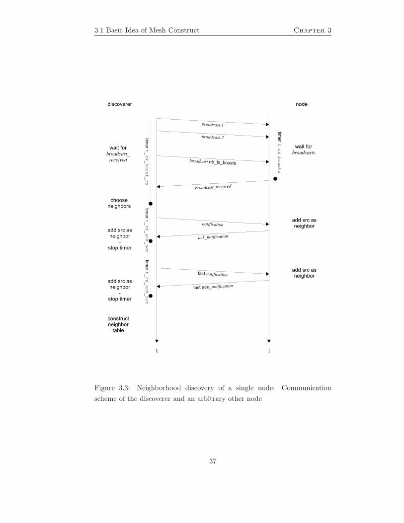
3.1 Basic Idea of Mesh Construct Chapter 3
Figure 3.3: Neighborhood discovery of a single node: Communication
scheme of the discoverer and an arbitrary other node
37

Chapter 3 Conceptual Design
cast received messages. When the timer t rx bcast rx expires, the dis-
coverer chooses the best nodes from the node tbl according to the choose
neighbors algorithm 5. The output of the algorithm is a list of chosen nodes.
Subsequently, the discoverer transmits a notification message to the the first
chosen node. Simultaneously, a timer t rx ack not is started at the discov-
erer. A node receiving a notification adds the source as neighbor to the
neighbor tbl and transmits an ack notification back to the discoverer. As
reaction on receiving an ack notification the discoverer adds the source as
neighbor as well, restarts t rx ack not and transmits a notification to the
next chosen node. Upon having received all ack notifications, the discoverer
constructs a neighbor table and thus the neighborhood discovery is com-
pleted.
Like in the Mesh Construct procedure timers and retry mechanisms with
thresholds for the number of retries are introduced to prevent the algorithm
from stopping in case of a lost message. E.g. while the timer t rx bcast rx
is running the discoverer waits for receiving broadcast received messages.
When t rx bcast rx expires and not a single broadcast received is received,
the discoverer transmits again a sequence of broadcasts if the number of re-
tries rtr bcast has not already exceeded the threshold rtr bcast max. If so,
no neighbors could be found with the neighborhood discovery. Analogously,
while the timer t rx ack not is running the discoverer waits for a particular
ack notification. When t rx ack not expires the discoverer retransmits the
notification if the number of retries rtr not for this node has not already
exeeded the threshold rtr not max. If so, new nodes are chosen if the number
of retries rtr choose has not already exceeded the threshold rtr choose max,
otherwise no additional neighbors could be found.
The neighborhood discovery is completed with the construction of the
neighbor table, whether it could be filled up with neighbors or remains
empty.
3.1.3 Choose Neighbors
The choose neighbors procedure is a component of the neighborhood discov-
ery. The procedure chooses neighbors among all nodes which are discovered
during the neighborhood discovery. The objective of the choose neighbors
procedure is to make the best choice for the purpose of the whole wireless
sensor network. The choose neighbors procedure is also described in the
38
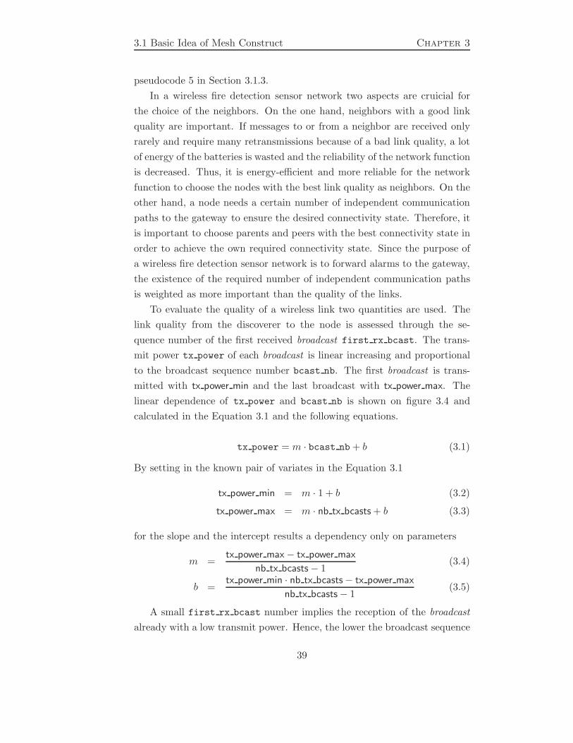
3.1 Basic Idea of Mesh Construct Chapter 3
pseudocode 5 in Section 3.1.3.
In a wireless fire detection sensor network two aspects are cruicial for
the choice of the neighbors. On the one hand, neighbors with a good link
quality are important. If messages to or from a neighbor are received only
rarely and require many retransmissions because of a bad link quality, a lot
of energy of the batteries is wasted and the reliability of the network function
is decreased. Thus, it is energy-efficient and more reliable for the network
function to choose the nodes with the best link quality as neighbors. On the
other hand, a node needs a certain number of independent communication
paths to the gateway to ensure the desired connectivity state. Therefore, it
is important to choose parents and peers with the best connectivity state in
order to achieve the own required connectivity state. Since the purpose of
a wireless fire detection sensor network is to forward alarms to the gateway,
the existence of the required number of independent communication paths
is weighted as more important than the quality of the links.
To evaluate the quality of a wireless link two quantities are used. The
link quality from the discoverer to the node is assessed through the se-
quence number of the first received broadcast first rx bcast. The trans-
mit power tx power of each broadcast is linear increasing and proportional
to the broadcast sequence number bcast nb. The first broadcast is trans-
mitted with tx power min and the last broadcast with tx power max. The
linear dependence of tx power and bcast nb is shown on figure 3.4 and
calculated in the Equation 3.1 and the following equations.
tx power = m · bcast nb + b (3.1)
By setting in the known pair of variates in the Equation 3.1
tx power min = m · 1 + b (3.2)
tx power max = m · nb tx bcasts + b (3.3)
for the slope and the intercept results a dependency only on parameters
m =tx power max − tx power max
nb tx bcasts − 1(3.4)
b =tx power min · nb tx bcasts − tx power max
nb tx bcasts − 1(3.5)
A small first rx bcast number implies the reception of the broadcast
already with a low transmit power. Hence, the lower the broadcast sequence
39

Chapter 3 Conceptual Design
Figure 3.4: linear increasing txpower
number the better is the link quality. To assess the link quality from the
node to the discoverer the received signal strength is measured and stored
in the variable rssi. By considering the link quality in both directions, the
choice of neighbors with an unsymmetric link quality shall be prevented.
The first rx bcast and rssi are message fields of the broadcast received
and are stored for each discovered node in the node table.
To make the best choice concerning the connectivity state the following
items from the node table are required for each node: number of peers nb pe,
connectivity state con state, hop count hop count, number of neighbors
nb nhs, and number of retries to transmit a notification rtr not. Addi-
tionaly, for the discoverer the following fields are required: own hop count
own hop count, own number of parents own nb pa, own number of peers
own nb pe, and own number of children own nb ch.
The choose neighbor procedure starts with a check of the node table.
Nodes which have already exceeded the threshold for the notification retries
(rtr not ≥ rtr not max) or have already a full neighbor table (nb nhs ≥
nb nhs max) are removed from the node table. Subsequently all nodes are
40

3.1 Basic Idea of Mesh Construct Chapter 3
sorted for the minimal first rx bcast and the maximal rssi. Thereby,
always the node with the better link quality is chosen, when two nodes
have the same ranking concerning the connectivity state. The discoverer
always tries to meet the requirements of the parameters concerning the
minimal number of parents, peers, or children on the corresponding hop
counts (pe hc1 min, pa hc2 min, ...). Moreover, the discoverer always checks
and only chooses a node if the own number of parents own nb pa, the own
number of peers own nb pe, and the own number of children own nb ch does
not already meet the requirements. In the following the choose neighbor
procedure distinguishs 4 different cases:
• own hop count = 0:
There is no connectivity state information at disposal of the gateway
at the start. The gateway choses the first nb nhs max nodes with the
best link quality from the node table.
• own hop count = 1:
The discoverer chooses the first pe hc1 min peers with minimal nb pe
to prevent that each discoverer with hop count 1 chooses the same
peers. Additionally, the required connectivity state is ensured. Then,
ch hc1 min children with a minimal con state are chosen in order to
add new nodes to the network and improve their connectivity state.
• own hop count = 2:
The discoverer chooses the first pa hc2 min parents with maximal con-
state to ensure the own required connectivity state. If not enough
parents can be chosen, additonal peers to the pe hc2 min with a maxi-
mal con state are chosen instead to ensure the own required connec-
tivity state. Then, ch hc2 min children with a minimal con state are
chosen in order to add new nodes to the network and improve their
connectivity state.
• own hop count = 3:
The discoverer chooses the first pa hc3 min parents with maximal con-
state to ensure the own required connectivity state. If not enough
parents can be chosen, additonal peers to the pe hc3 min with a maxi-
mal con state are chosen instead to ensure the own required connec-
tivity state. If not already chosen, pe hc3 min children with a minimal
con state are chosen in order to improve their connectivity state.
41

Chapter 3 Conceptual Design
At the end of the procedure the list of the chosen nodes is truncated to
the number of neighbors which can maximally be added. For that reason,
only the first (nb nhs max - own nb nhs) nodes are returned as the list of
chosen neighbors.
3.2 Node Functions and Fields
In this section the three different node functions and their corresponding
fields are described in more detail. The three different node types are de-
noted as gateway, discoverer, and node functionality.
3.2.1 Gateway
It is assumed that only one node with the gateway functionality exists in
the entire network. More gateways in one single network are conceivable but
in the scope of this thesis only networks with one gateway are investigated.
However, the gateway implements also the discoverer and node functionality.
The gateway controls and monitors the whole Mesh Construct procedure.
In particular, the start, the proceeding temporal non-overlapping neighbor-
hood discoveries, and the termination i. e. the start of the topology control
are initiated by the gateway. Besides, the gateway constructs and maintains
a discoverer table, wherein informations about each node in the network are
stored. For that reason, several additional variables and fields are required
in the gateway and listed in the Table 3.1 and Table 3.2.
The discoverer table discoverer tbl contains the node address nd add
and the connectivity state con state. The node address indentifies the
different discoverers and the connectivity state is required to track the con-
nectivity state of the entire network. Besides, nd add and con state in the
discoverer table for each discoverer the hop count and a trace are stored.
For example these informations are required to initiate a neighborhood dis-
covery. In a trace the addresses of the nodes on the communication path
between the gateway and the discoverer are stored. The combination of
the trace and the hop count allows to transmit a DSR message from the
gateway to the discoverer over more than one hop. The DSR messages are
described more detailed in Section 3.3.3.
The discoverer index discoverer ind indicates the discoverer in the
discoverer tbl, which is currently performing a neighborhood discovery.
42

3.2 Node Functions and Fields Chapter 3
Gateway Gateway variable description
discoverer tbl Discoverer table with informations of all
discoverer nodes (see Table 3.2)
discoverer ind Indicates the current discoverer node
mc state The Mesh Construct state indicates on which
hop count the current discoverer is performing
the neighborhood discovery
nb nds on hc Number of discovered nodes on
the current mc state
nb rx nhtbl Number of received neighbor tables on the
current mc state (see Table 3.6)
rtr start Number of retries for transmitting a start discovery
to the current discoverer
rtr request Number of retries for transmitting a
request neighbor table to the current discoverer
rtr completed Number of retries for transmitting a
completed to the current discoverer
Table 3.1: Variables of the gateway
discoverer tbl discoverer tbl variable description
nd add Node address of the discoverer
con state Connectivity state of the discoverer
hop count Hopcount of the discoverer
trace The list of node addresses of one communication
path from the gateway to the discoverer
Table 3.2: Variables for each discoverer entry of the discvoerer table
43
Chapter 3 Conceptual Design
The Mesh Construct state mc state indicates the hop count of the cur-
rent discoverer discoverer ind. The number of nodes nb nds on hc on the
current Mesh Construct state is set each time the mc state is incremented
according the hop count informations in the discoverer table. The num-
ber of received neighbor tables nb rx nhtbl is incremented if the expected
neighbor table is received. The variables rtr start and rtr request are
required to count the corresponding retries.
3.2.2 Discoverer
The discoverer functionality is contained in each node of the network, since
each node has to perform at least one neighborhood discovery. The task
of a discoverer consists of discovering and choosing neighbors. The chosen
neighbors are notified and subsequently added to the neighbor table in case
an ack notification is received. The neighbor table is transmitted to the
gateway to deliver the information about the mesh network topology. The
variables and fields required in the discoverer are listed in the Table 3.3 and
Table 3.4.
For deciding which neighboring nodes to choose as neighbors the dis-
coverer for each discovered node stores information contained in the broad-
cast received messages in a node table node tbl. How a discoverer chooses
nodes depending on the values of the fields in the node table is described in
Section 3.1.3.
The number of received broadcast received messages nb rx bcast rx is
incremented at the reception of a broadcast received and is required to de-
termine if no nodes at all are beeing discovered. After neighbors have been
chosen the number of notifications to transmit nb tx notifications is set
in order to be able to decide wether all expected ack notifications are re-
ceived. The variables rtr bcast and rtr choose are required to count the
corresponding retries.
3.2.3 Node
The node functionality is the basic functionality contained in each node of
the mesh network. A node is only reacting on certain events: broadcasts are
answered with broadcast received, notifications are answered with notifica-
tions, and DSR messages are forwarded if required. Nodes are passive as
44
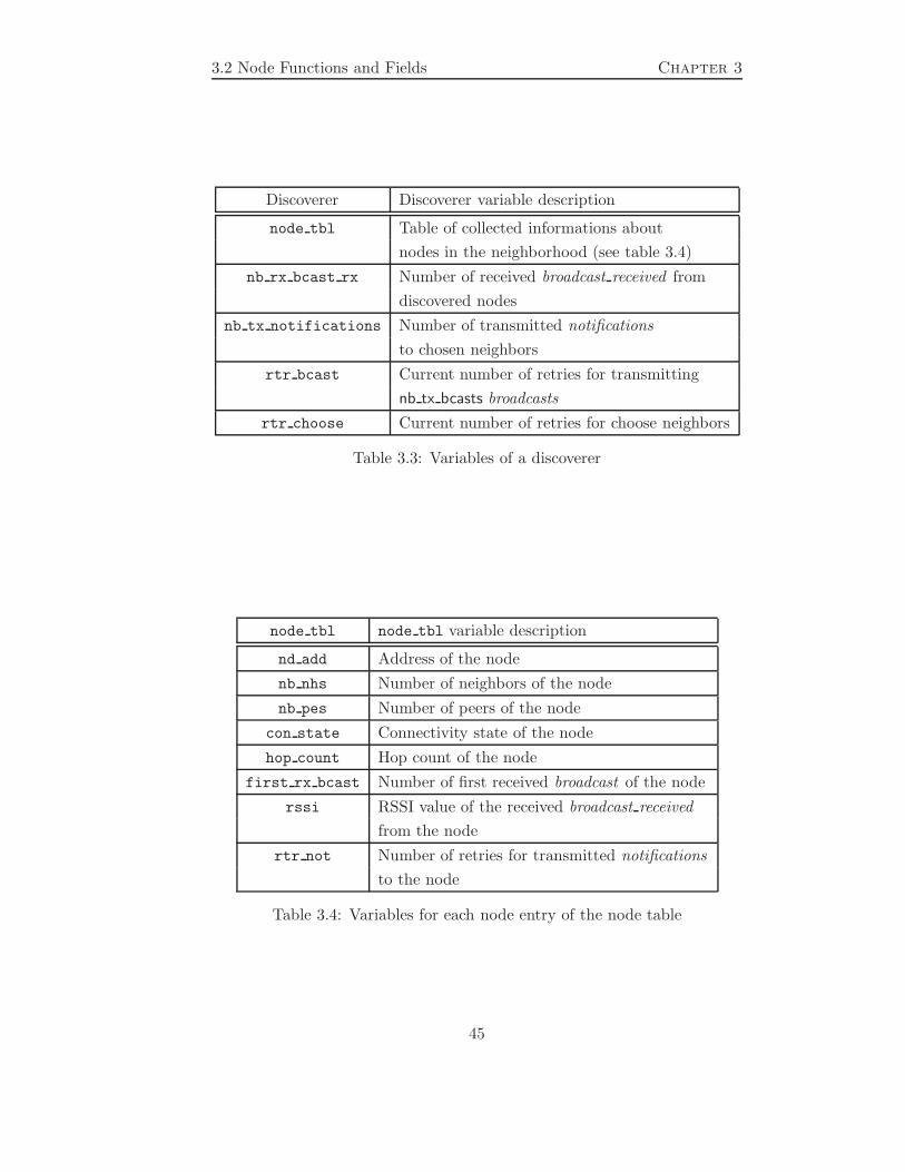
3.2 Node Functions and Fields Chapter 3
Discoverer Discoverer variable description
node tbl Table of collected informations about
nodes in the neighborhood (see table 3.4)
nb rx bcast rx Number of received broadcast received from
discovered nodes
nb tx notifications Number of transmitted notifications
to chosen neighbors
rtr bcast Current number of retries for transmitting
nb tx bcasts broadcasts
rtr choose Current number of retries for choose neighbors
Table 3.3: Variables of a discoverer
node tbl node tbl variable description
nd add Address of the node
nb nhs Number of neighbors of the node
nb pes Number of peers of the node
con state Connectivity state of the node
hop count Hop count of the node
first rx bcast Number of first received broadcast of the node
rssi RSSI value of the received broadcast received
from the node
rtr not Number of retries for transmitted notifications
to the node
Table 3.4: Variables for each node entry of the node table
45
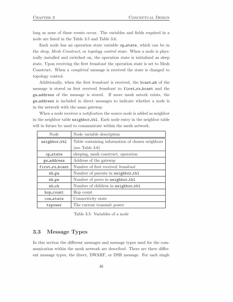
Chapter 3 Conceptual Design
long as none of these events occur. The variables and fields required in a
node are listed in the Table 3.5 and Table 3.6.
Each node has an operation state variable op state, which can be in
the sleep, Mesh Construct, or topology control state. When a node is phys-
ically installed and switched on, the operation state is initialized as sleep
state. Upon receiving the first broadcast the operation state is set to Mesh
Construct. When a completed message is received the state is changed to
topology control.
Additionally, when the first broadcast is received, the bcast nb of the
message is stored as first received broadcast to first rx bcast and the
gw address of the message is stored. If more mesh netork exists, the
gw address is included in direct messages to indicate whether a node is
in the network with the same gateway.
When a node receives a notification the source node is added as neighbor
in the neighbor table neighbor tbl. Each node entry in the neighbor table
will in future be used to communicate within the mesh network.
Node Node variable description
neighbor tbl Table containing information of chosen neighbors
(see Table 3.6)
op state sleeping, mesh construct, operation
gw address Address of the gateway
first rx bcast Number of first received broadcast
nb pa Number of parents in neighbor tbl
nb pe Number of peers in neighbor tbl
nb ch Number of children in neighbor tbl
hop count Hop count
con state Connectivity state
txpower The current transmit power
Table 3.5: Variables of a node
3.3 Message Types
In this section the different messages and message types used for the com-
munication within the mesh network are described. There are three differ-
ent message types, the direct, DWARF, or DSR message. For each single
46

3.3 Message Types Chapter 3
neighbor tbl neighbor tbl variable description
nd add Node address of the neighbor
con state Connectivity state of the neighbor
hop count Hop count of the neighbor
Table 3.6: Variables for each neighbor entry of the neighbor table
message it is indicated between which node types it is transmitted, which
information is contained, in which situations the message is sent, and which
actions are performed when the message is received. Each message con-
tains the message type, the destination address, and the source address as
message fields.
3.3.1 Direct Messages
Direct messages are exchanged over a distance of one hop. There are unicast
messages from one node to another or a broadcast message from one node
to all nodes in communcation range.
broadcast
A broadcast is transmitted from a discoverer to all nodes in communication
range. The information fields contained in a broadcast are listed in the Table
3.7.
broadcast broadcast field description
msg type Identifier indicating the message type broadcast
dest bcast Destination address
src bcast Source address
bcast nb Sequence number of the broadcast
gw address Gateway address
Table 3.7: Message fields of a broadcast
The broadcast message is transmitted nb tx bcast times with linear in-
creasing transmit power at the beginning of a neighborhood discovery. The
broadcast sequence number is incremented after each transmission.
When a node receives the first broadcast from a discoverer, the broad-
cast sequence number bcast nb is stored to first rx bcast and the timer
47
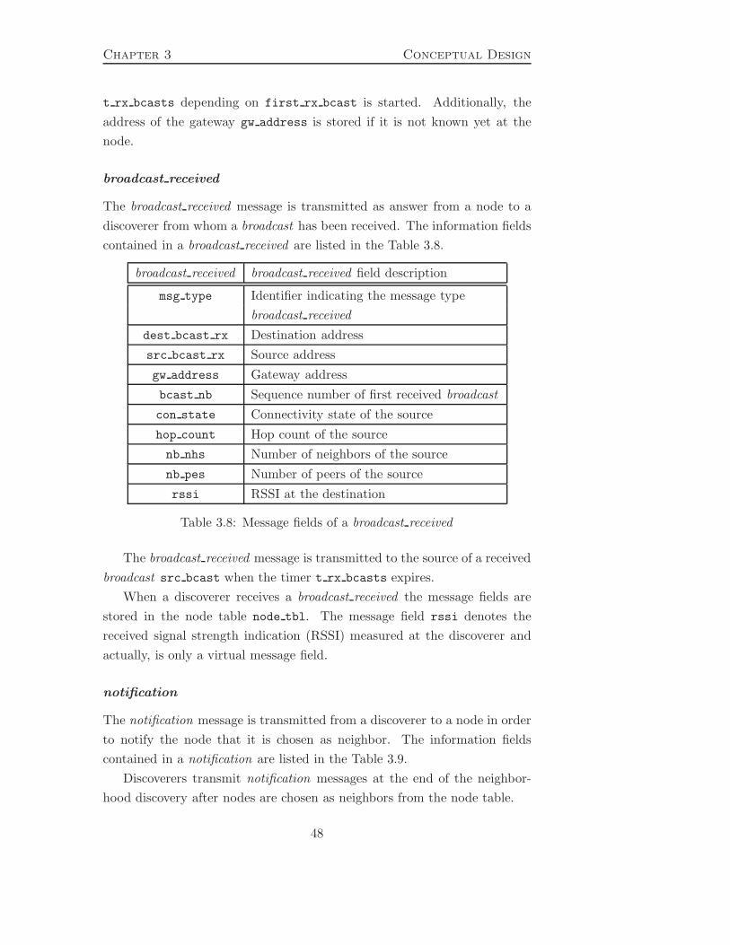
Chapter 3 Conceptual Design
t rx bcasts depending on first rx bcast is started. Additionally, the
address of the gateway gw address is stored if it is not known yet at the
node.
broadcast received
The broadcast received message is transmitted as answer from a node to a
discoverer from whom a broadcast has been received. The information fields
contained in a broadcast received are listed in the Table 3.8.
broadcast received broadcast received field description
msg type Identifier indicating the message type
broadcast received
dest bcast rx Destination address
src bcast rx Source address
gw address Gateway address
bcast nb Sequence number of first received broadcast
con state Connectivity state of the source
hop count Hop count of the source
nb nhs Number of neighbors of the source
nb pes Number of peers of the source
rssi RSSI at the destination
Table 3.8: Message fields of a broadcast received
The broadcast received message is transmitted to the source of a received
broadcast src bcast when the timer t rx bcasts expires.
When a discoverer receives a broadcast received the message fields are
stored in the node table node tbl. The message field rssi denotes the
received signal strength indication (RSSI) measured at the discoverer and
actually, is only a virtual message field.
notification
The notification message is transmitted from a discoverer to a node in order
to notify the node that it is chosen as neighbor. The information fields
contained in a notification are listed in the Table 3.9.
Discoverers transmit notification messages at the end of the neighbor-
hood discovery after nodes are chosen as neighbors from the node table.
48
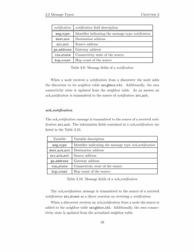
3.3 Message Types Chapter 3
notification notification field description
msg type Identifier indicating the message type notification
dest not Destination address
src not Source address
gw address Gateway address
con state Connectivity state of the source
hop count Hop count of the source
Table 3.9: Message fields of a notification
When a node receives a notification from a discoverer the node adds
the discoverer to its neighbor table neighbor tbl. Additionally, the own
connectivity state is updated from the neighbor table. As an answer an
ack notification is transmitted to the source of notification src not.
ack notification
The ack notification message is transmitted to the source of a received noti-
fication src not. The information fields contained in a ack notification are
listed in the Table 3.10.
Variable Variable description
msg type Identifier indicating the message type ack notification
dest ack not Destination address
src ack not Source address
gw address Gateway address
con state Connectivity state of the source
hop count Hop count of the source
Table 3.10: Message fields of a ack notification
The ack notification message is transmitted to the source of a received
notification src bcast as a direct reaction on receiving a notification.
When a discoverer receives an ack notification from a node the source is
added to the neighbor table neighbor tbl. Additionally, the own connec-
tivity state is updated from the actualized neighbor table.
49
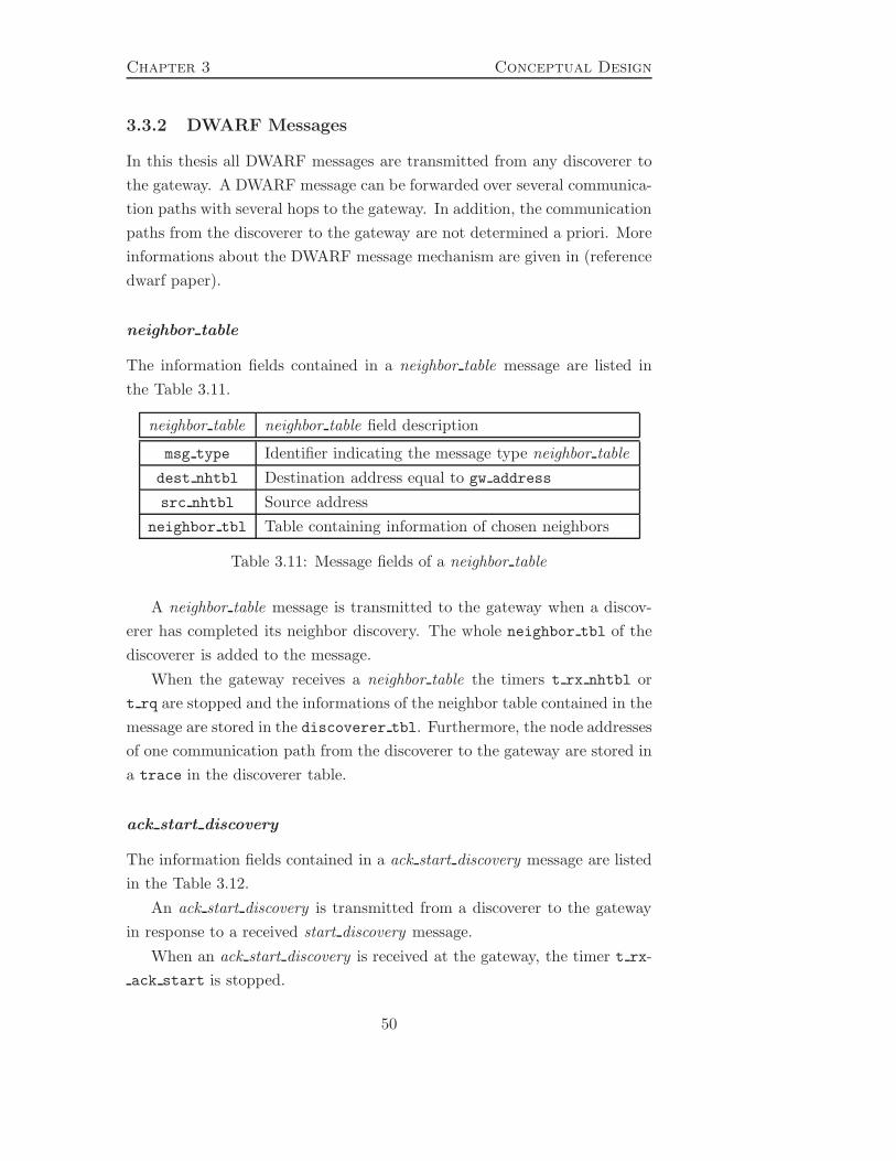
Chapter 3 Conceptual Design
3.3.2 DWARF Messages
In this thesis all DWARF messages are transmitted from any discoverer to
the gateway. A DWARF message can be forwarded over several communica-
tion paths with several hops to the gateway. In addition, the communication
paths from the discoverer to the gateway are not determined a priori. More
informations about the DWARF message mechanism are given in (reference
dwarf paper).
neighbor table
The information fields contained in a neighbor table message are listed in
the Table 3.11.
neighbor table neighbor table field description
msg type Identifier indicating the message type neighbor table
dest nhtbl Destination address equal to gw address
src nhtbl Source address
neighbor tbl Table containing information of chosen neighbors
Table 3.11: Message fields of a neighbor table
A neighbor table message is transmitted to the gateway when a discov-
erer has completed its neighbor discovery. The whole neighbor tbl of the
discoverer is added to the message.
When the gateway receives a neighbor table the timers t rx nhtbl or
t rq are stopped and the informations of the neighbor table contained in the
message are stored in the discoverer tbl. Furthermore, the node addresses
of one communication path from the discoverer to the gateway are stored in
a trace in the discoverer table.
ack start discovery
The information fields contained in a ack start discovery message are listed
in the Table 3.12.
An ack start discovery is transmitted from a discoverer to the gateway
in response to a received start discovery message.
When an ack start discovery is received at the gateway, the timer t rx-
ack start is stopped.
50
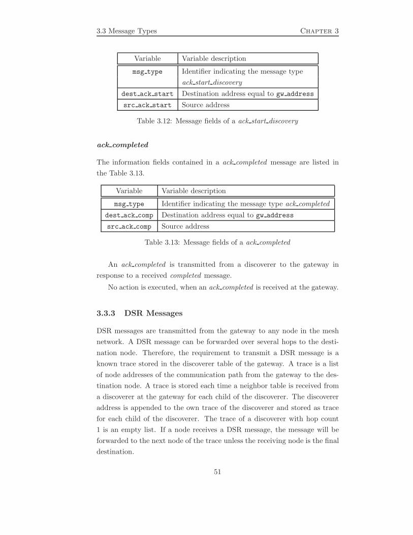
3.3 Message Types Chapter 3
Variable Variable description
msg type Identifier indicating the message type
ack start discovery
dest ack start Destination address equal to gw address
src ack start Source address
Table 3.12: Message fields of a ack start discovery
ack completed
The information fields contained in a ack completed message are listed in
the Table 3.13.
Variable Variable description
msg type Identifier indicating the message type ack completed
dest ack comp Destination address equal to gw address
src ack comp Source address
Table 3.13: Message fields of a ack completed
An ack completed is transmitted from a discoverer to the gateway in
response to a received completed message.
No action is executed, when an ack completed is received at the gateway.
3.3.3 DSR Messages
DSR messages are transmitted from the gateway to any node in the mesh
network. A DSR message can be forwarded over several hops to the desti-
nation node. Therefore, the requirement to transmit a DSR message is a
known trace stored in the discoverer table of the gateway. A trace is a list
of node addresses of the communication path from the gateway to the des-
tination node. A trace is stored each time a neighbor table is received from
a discoverer at the gateway for each child of the discoverer. The discoverer
address is appended to the own trace of the discoverer and stored as trace
for each child of the discoverer. The trace of a discoverer with hop count
1 is an empty list. If a node receives a DSR message, the message will be
forwarded to the next node of the trace unless the receiving node is the final
destination.
51

Chapter 3 Conceptual Design
start discovery
The information fields contained in a start discovery message are listed in
the Table 3.14.
Variable Variable description
msg type Identifier indicating the message type start discovery
dest start Destination address equal to gw address
trace Node addresses to the destination node
src start Source address
Table 3.14: Message fields of a start discovery
A start discovery message is transmitted from the gateway to a discov-
erer to initiate the start of a neighborhood discovery.
When a start discovery message is received at a discoverer, an ack start-
discovery message is transmitted to the gateway to confirm the reception.
Subsequently, the neighborhood discovery procedure is started.
request neighbor table
The information fields contained in a request neighbor table message are
listed in the Table 3.15.
Variable Variable description
msg type Identifier indicating the message type
request neighbor table
dest rq nhtbl Destination address equal to gw address
trace Node addresses to the destination node
src rq nhtl Source address
Table 3.15: Message fields of a request neighbor table
A request neighbor table message is transmitted from the gateway to a
discover when the timer t rx nhtbl or t rq is expired before a neighbor
table is received from the discoverer at the gateway.
In response of receiving a request neighbor table a discoverer transmits
the requested neighbor table message to the gateway.
52
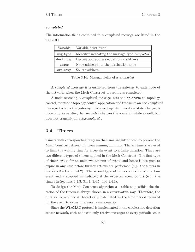
3.4 Timers Chapter 3
completed
The information fields contained in a completed message are listed in the
Table 3.16.
Variable Variable description
msg type Identifier indicating the message type completed
dest comp Destination address equal to gw address
trace Node addresses to the destination node
src comp Source address
Table 3.16: Message fields of a completed
A completed message is transmitted from the gateway to each node of
the network, when the Mesh Construct procedure is completed.
A node receiving a completed message, sets the op state to topology
control, starts the topology control application and transmits an ack completed
message back to the gateway. To speed up the operation state change, a
node only forwarding the completed changes the operation state as well, but
does not transmit an ack completed .
3.4 Timers
Timers with corresponding retry mechanisms are introduced to prevent the
Mesh Construct Algorithm from running infinitely. The set timers are used
to limit the waiting time for a certain event to a finite duration. There are
two different types of timers applied in the Mesh Construct. The first type
of timers waits for an unknown amount of events and hence is designed to
expire in any case before further actions are performed (e.g. the timers in
Sections 3.4.1 and 3.4.2). The second type of timers waits for one certain
event and is stopped immediately if the expected event occurs (e.g. the
timers in Sections 3.4.3, 3.4.4, 3.4.5, and 3.4.6).
To design the Mesh Construct algorithm as stable as possible, the du-
ration of the timers is always chosen in a conservative way. Therefore, the
duration of a timer is theoretically calculated as the time period required
for the event to occur in a worst case scenario.
Since the WiseMAC protocol is implemented in the wireless fire detection
sensor network, each node can only receive messages at every periodic wake
53

Chapter 3 Conceptual Design
up point. The constant time period between these wake up points is denoted
as the wake up period t w. Thus, the duration of each timer is determined
by a number of time slots t w. For further informations about the WiseMAC
protocol see (ref wisemac).
Figure 3.5: Scheme for transmitting a direct message
To determine the duration of certain timers, the duration for the trans-
mission of one direct message is required. The possible worst case situation
of a direct transmission is illustrated in the Figure 3.5. A message is en-
queued in a node for transmission an infinitesimal time after the wake up
point of the destination node. The transmitting node has to wait the re-
maining time for its own wake up point t s plus the time difference between
the wake up patterns of both nodes t d until the transmission of the message
can be started. Depending on the length of the message t m the total dura-
tion t total from the point where the message is enqueued for transmission
until it is entirely received at the destination node is possibly longer than
one wake up period t w.
t total = t s + t d + t m > t w (3.6)
Therefore, the assumed time duration for transmitting a direct message is
54

3.4 Timers Chapter 3
rounded up to two wake up periods.
t direct = 2 · t w (3.7)
As a consequence of equation 3.7 the maximal duration for the transmission
of a DWARF oder DSR message is given by the maximal number of hops.
t dwarf = nb hops max · t direct
= 2 · nb hops max · t w (3.8)
t dsr = nb hops max · t direct
= 2 · nb hops max · t w (3.9)
In the following sections for each timer the derivation of the duration is
described. Moreover, for each timer the starting point, the event the timer
waits for, and the actions which will be performed at the timer stop or
expiration are indicated.
3.4.1 Timeout receive broadcasts t rx bcasts
The timer t rx bcasts is started when the first broadcast of a discov-
erer is completely received at a node. While the timer t rx bcasts is
running, the node waits for the reception of the remaining (nb tx bcasts
- first rx bcast) broadcasts of the discoverer. When the timer expires the
node transmits a broadcast received to the discoverer.
Due to a technical restriction it is not possible to transmit broadcasts in
consecutive time slots. A number of idle slots has to be inserted between the
transmission of two broadcasts. During the transmission of the broadcast se-
quence the reception of a broadcast received at the discoverer is complicated
or not possible. Thus, the node transmits the broadcast received message
only after the last broadcast is received. Since each node in communica-
tion range receives the last broadcast approximately at the same time, a
simultaneous transmission of the broadcast received to the gateway leads to
numerous collisions at the gateway. For that reason a random number of
time slots t w is added to the timer duration in order to decrease the num-
ber of collisions. The random number is uniformly distributed over the set
{0, nb nds}. The scheme for the duration of the timer t rx bcasts is shown
in the Figure 3.6.
55

Chapter 3 Conceptual Design
t rx bcast (first rx bcast) = [(nb tx bcasts − first rx bcast)
· (idle slots + 1)
+ random(0, nb nds)] · t w (3.10)
Figure 3.6: Scheme for the duration of the timer t rx bcast
3.4.2 Timeout receive broadcast-received t rx bcast rx
The timer t rx bcast rx is started when the discoverer starts the transmis-
sion of the first broadcast of the sequence. While the timer t rx bcast rx
is running, the discoverer waits for the reception of broadcast received mes-
sages. When the timer expires the discoverer starts the choose neighbors
algorithm.
The scheme for the duration of the timer t rx bcast rx is shown in
the Figure 3.7. The duration of the timer t rx bcast rx is composed of
the time required for transmitting the broadcast sequence t bcast seq and
the random time waited of the nodes t wait to reduce collisons. From the
Figure 3.7 the duration of the t bcast seq results
t bcast seq = [1 + (nb tx bcasts − 1) · (idle slots + 1)] · t w (3.11)
56

3.4 Timers Chapter 3
If the worst case is assumed the t wait is equal to the maximal waiting time
slots
t wait = nb nds · t w (3.12)
The total duration of the timer t rx bcast rx results as
t rx bcast rx = t bcast seq+ t wait (3.13)
= [(nb tx bcasts − 1) · (idle slots + 1)
+1 + nb nds] · t w (3.14)
Figure 3.7: Scheme for the duration of the timer t rx bcast rx
3.4.3 Timeout receive ack-notification t rx ack not
The timer t rx ack not is started when a discoverer transmits a notification
to a chosen node. While the timer t rx ack not is running, the discoverer
waits for an ack notification from the chosen node. When an ack notification
is received at the discoverer, the timer is stopped. If the timer expires,
another notification is transmitted to the node unless the number of retries
57

Chapter 3 Conceptual Design
rtr not has not exceeded the threshold rtr not max. If the threshold is
exceeded, new neighbors are chosen an notified with a notification.
Since notifications and ack notifications are transmitted only over one
hop, the duration of the timer t rx ack not is equal to the time required
to transmit two direct messages.
t rx ack not = 2 · t direct (3.15)
= 4 · t w (3.16)
3.4.4 Timeout receive ack-start-discovery t rx ack start
The timer t rx ack start is started when the gateway transmits a start-
discovery to a discoverer. While the timer t rx ack not is running, the
gateway waits for an ack start message from the discoverer. When an
ack start is received at the gateway, the timer is stopped. If the timer
expires, another start discovery is transmitted to the discoverer unless the
number of retries rtr start has not exceeded the threshold rtr start max. If
the threshold is exceeded, the start of the discovery failed and a start discovery
is transmitted to the next discoverer.
Start discovery and ack start messages are transmitted over several hops.
The start discovery is a DSR message and the ack start is a DWARF mes-
sage. Therefore, the duration of the timer t rx ack start is equal to the
time required to transmit a DSR and a DWARF message.
t rx ack start = t dsr+ t dwarf (3.17)
= 2 · nb hops max · t direct (3.18)
= 4 · nb hops max · t w (3.19)
3.4.5 Timeout receive neighbor-table t rx nhtbl
The timer t rx nhtbl is started when the gateway transmits a start discovery
to a discoverer. While the timer t rx nhtbl is running, the gateway waits
for a neighbor table message from the discoverer. When a neighbor table
is received at the gateway, the timer is stopped. If the timer expires,
a request nhtbl is transmitted to the discoverer unless the number of re-
tries rtr request has not exceeded the threshold rtr request max. If the
58
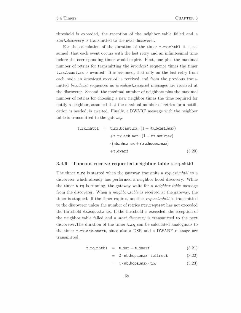
3.4 Timers Chapter 3
threshold is exceeded, the reception of the neighbor table failed and a
start discovery is transmitted to the next discoverer.
For the calculation of the duration of the timer t rx nhtbl it is as-
sumed, that each event occurs with the last retry and an infinitesimal time
before the corresponding timer would expire. First, one plus the maximal
number of retries for transmitting the broadcast sequence times the timer
t rx bcast rx is awaited. It is assumed, that only on the last retry from
each node an broadcast received is received and from the previous trans-
mitted broadcast sequences no broadcast receiced messages are received at
the discoverer. Second, the maximal number of neighbors plus the maximal
number of retries for choosing a new neighbor times the time required for
notify a neighbor, assumed that the maximal number of retries for a notifi-
cation is needed, is awaited. Finally, a DWARF message with the neighbor
table is transmitted to the gateway.
t rx nhtbl = t rx bcast rx · (1 + rtr bcast max)
+t rx ack not · (1 + rtr not max)
· (nb nhs max + rtr choose max)
+t dwarf (3.20)
3.4.6 Timeout receive requested-neighbor-table t rq nhtbl
The timer t rq is started when the gateway transmits a request nhtbl to a
discoverer which already has performed a neighbor hood discovery. While
the timer t rq is running, the gateway waits for a neighbor table message
from the discoverer. When a neighbor table is received at the gateway, the
timer is stopped. If the timer expires, another request nhtbl is transmitted
to the discoverer unless the number of retries rtr request has not exceeded
the threshold rtr request max. If the threshold is exceeded, the reception of
the neighbor table failed and a start discovery is transmitted to the next
discoverer.The duration of the timer t rq can be calculated analoguous to
the timer t rx ack start, since also a DSR and a DWARF message are
transmitted.
t rq nhtbl = t dsr + t dwarf (3.21)
= 2 · nb hops max · t direct (3.22)
= 4 · nb hops max · t w (3.23)
59

Chapter 3 Conceptual Design
3.5 Parameters
Paramter Parameter description
nb nds Total number of nodes
nb nhs max Maximal number of neighbors per node
nb hops max Maximal number of hops in the network
nb con paths min Minimal number of independent communication
paths from a detector to the gateway
nb tx bcasts Number of broadcasts a discoverer transmits
t w Wake up period of the Wisemac
idle slots Technical required idle time between
transmitting a message
tx power min Minimal transmit power
tx power max Maximal transmit power
rtr bcast max Maximal number of retries for transmitting
nb tx bcasts broadcasts
rtr choose max Maximal number of retries for choose neighbors
rtr not max Maximal number of retries for
transmitting a notification to a particular node
rtr start max Maximal number of retries for
transmitting a start
rtr request max Maximal number for transmitting
an request neighbor table
pe hc1 min Minimal number of peers on hopcount 1
ch hc1 min Minimal number of children on hopcount 1
pa hc2 min Minimal number of parents on hopcount 2
pe hc2 min Minimal number of peers on hopcount 2
ch hc2 min Minimal number of children on hopcount 2
pa hc3 min Minimal number of parents on hopcount 3
pe hc3 min Minimal number of peers on hopcount 3
Table 3.17: Parameters of Mesh Construct
60
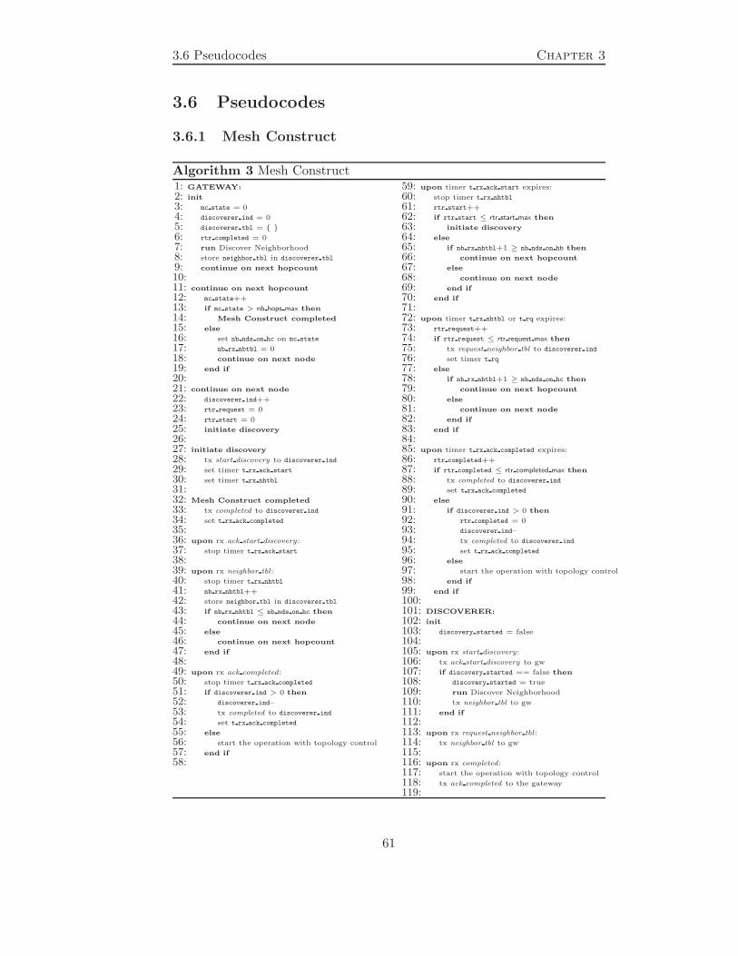
3.6 Pseudocodes Chapter 3
3.6 Pseudocodes
3.6.1 Mesh Construct
Algorithm 3 Mesh Construct1: GATEWAY:
2: init
3: mc state = 0
4: discoverer ind = 0
5: discoverer tbl = { }
6: rtr completed = 0
7: run Discover Neighborhood
8: store neighbor tbl in discoverer tbl
9: continue on next hopcount
10:
11: continue on next hopcount
12: mc state++
13: if mc state > nb hops max then
14: Mesh Construct completed
15: else
16: set nb nds on hc on mc state
17: nb rx nbtbl = 0
18: continue on next node
19: end if
20:
21: continue on next node
22: discoverer ind++
23: rtr request = 0
24: rtr start = 0
25: initiate discovery
26:
27: initiate discovery
28: tx start discovery to discoverer ind
29: set timer t rx ack start
30: set timer t rx nhtbl
31:
32: Mesh Construct completed
33: tx completed to discoverer ind
34: set t rx ack completed
35:
36: upon rx ack start discovery:
37: stop timer t rx ack start
38:
39: upon rx neighbor tbl:
40: stop timer t rx nhtbl
41: nb rx nhtbl++
42: store neighbor tbl in discoverer tbl
43: if nb rx nhtbl ≤ nb nds on hc then
44: continue on next node
45: else
46: continue on next hopcount
47: end if
48:
49: upon rx ack completed:
50: stop timer t rx ack completed
51: if discoverer ind > 0 then
52: discoverer ind–
53: tx completed to discoverer ind
54: set t rx ack completed
55: else
56: start the operation with topology control
57: end if
58:
59: upon timer t rx ack start expires:
60: stop timer t rx nhtbl
61: rtr start++
62: if rtr start ≤ rtr start max then
63: initiate discovery
64: else
65: if nb rx nhtbl+1 ≥ nb nds on hb then
66: continue on next hopcount
67: else
68: continue on next node
69: end if
70: end if
71:
72: upon timer t rx nhtbl or t rq expires:
73: rtr request++
74: if rtr request ≤ rtr request max then
75: tx request neighbor tbl to discoverer ind
76: set timer t rq
77: else
78: if nb rx nhtbl+1 ≥ nb nds on hc then
79: continue on next hopcount
80: else
81: continue on next node
82: end if
83: end if
84:
85: upon timer t rx ack completed expires:
86: rtr completed++
87: if rtr completed ≤ rtr completed max then
88: tx completed to discoverer ind
89: set t rx ack completed
90: else
91: if discoverer ind > 0 then
92: rtr completed = 0
93: discoverer ind–
94: tx completed to discoverer ind
95: set t rx ack completed
96: else
97: start the operation with topology control
98: end if
99: end if
100:
101: DISCOVERER:
102: init
103: discovery started = false
104:
105: upon rx start discovery:
106: tx ack start discovery to gw
107: if discovery started == false then
108: discovery started = true
109: run Discover Neighborhood
110: tx neighbor tbl to gw
111: end if
112:
113: upon rx request neighbor tbl:
114: tx neighbor tbl to gw
115:
116: upon rx completed:
117: start the operation with topology control
118: tx ack completed to the gateway
119:
61

Chapter 3 Conceptual Design
3.6.2 Neighborhood Discovery
Algorithm 4 Neighborhood Discovery1: DISCOVERER:
2: init
3: nb rx bcast rx = 0
4: node tbl = {}
5: NbRxAckNot = 0
6: rtr bcast = 0
7: rtr choose = 0
8: start
9:
10: start
11: set timer t rx bcast rx
12: for bcastnb = 1 to nb tx bcast do
13: txpower = m · bcastnb + b
14: tx broadcast(txpower,bcastnb)
15: wait idle slots
16: end for
17:
18: upon rx broadcast received:
19: nb rx bcast rx++
20: add src bcast rx to node tbl
21:
22: upon rx ack notification:
23: add src ack not to neighbor tbl
24: stop timer t rx ack not
25: NbRxAckNot++
26: if NbRxAckNot ≥ nb tx notifications then
27: //neighborhood discovery completed
28: return neighbor tbl
29: else
30: chosen node++
31: tx notification
32: end if
33:
34: upon timer t rx bcast rx expires:
35: if nb rx bcast rx == 0 then
36: rtr bcast++
37: if rtr bcast ≤ rtr bcast max then
38: //restart discovery
39: go to start
40: else
41: //No neighbors found
42: return neighbor tbl
43: end if
44: else
45: run Choose Neighbors
46: set nb tx notifications
47: tx notification
48: end if
49:
50: upon timer t rx ack not expires:
51: chosen node.rtr not++
52: if chosen node.rtr not ≤ rtr not max then
53: tx notification
54: else
55: rtr choose++
56: if rtr choose ≤ rtr choose max then
57: run Choose Neighbors
58: NbRxAckNot = 0
59: set nb tx notifications
60: if nb tx notifications == 0 then
61: //No neighbors are chosen
62: return neighbor tbl
63: else
64: tx notification
65: end if
66: else
67: //No additional neighbors found
68: return neighbor tbl
69: end if
70: end if
71:
72: tx notification
73: tx notification to chosen node
74: set timer t rx ack not
75:
76: NODE:
77: init
78: first rx bcast = 0
79: neighbor tbl ={}
80:
81: upon rx broadcast(bcast nb):
82: if first rx bcast == 0 then
83: first rx bcast = bcast nb
84: discoverer add = src bcast
85: set timer t rx bcast(first rx bcast)
86: end if
87:
88: upon rx notification:
89: add src not to neighbor tbl
90: tx ack notification to src not
91:
92: upon timer t rx bcast expires:
93: tx broadcast received(first rx bcast) to
discoverer add
94: first rx bcast = 0
95:
62
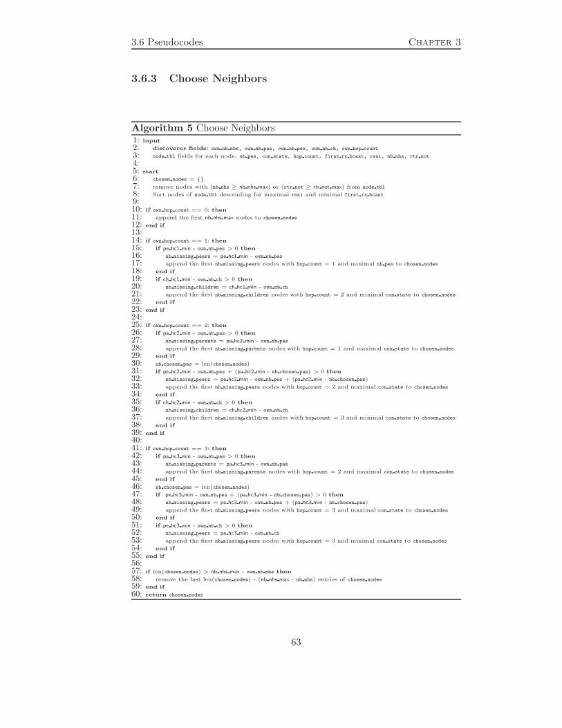
3.6 Pseudocodes Chapter 3
3.6.3 Choose Neighbors
Algorithm 5 Choose Neighbors1: input
2: discoverer fields: own nb nbs, own nb pas, own nb pes, own nb ch, own hop count
3: node tbl fields for each node: nb pes, con state, hop count, first rx bcast, rssi, nb nhs, rtr not
4:
5: start
6: chosen nodes = {}
7: remove nodes with (nb nhs ≥ nb nhs max) or (rtr not ≥ rtr not max) from node tbl
8: Sort nodes of node tbl descending for maximal rssi and minimal first rx bcast
9:
10: if own hop count == 0: then
11: append the first nb nhs max nodes to chosen nodes
12: end if
13:
14: if own hop count == 1: then
15: if pe hc1 min - own nb pes > 0 then
16: nb missing peers = pe hc1 min - own nb pes
17: append the first nb missing peers nodes with hop count = 1 and minimal nb pes to chosen nodes
18: end if
19: if ch hc1 min - own nb ch > 0 then
20: nb missing children = ch hc1 min - own nb ch
21: append the first nb missing children nodes with hop count = 2 and minimal con state to chosen nodes
22: end if
23: end if
24:
25: if own hop count == 2: then
26: if pa hc2 min - own nb pas > 0 then
27: nb missing parents = pa hc2 min - own nb pas
28: append the first nb missing parents nodes with hop count = 1 and maximal con state to chosen nodes
29: end if
30: nb chosen pas = len(chosen nodes)
31: if pe hc2 min - own nb pes + (pa hc2 min - nb chosen pas) > 0 then
32: nb missing peers = pe hc2 min - own nb pes + (pa hc2 min - nb chosen pas)
33: append the first nb missing peers nodes with hop count = 2 and maximal con state to chosen nodes
34: end if
35: if ch hc2 min - own nb ch > 0 then
36: nb missing children = ch hc2 min - own nb ch
37: append the first nb missing children nodes with hop count = 3 and minimal con state to chosen nodes
38: end if
39: end if
40:
41: if own hop count == 3: then
42: if pa hc3 min - own nb pas > 0 then
43: nb missing parents = pa hc3 min - own nb pas
44: append the first nb missing parents nodes with hop count = 2 and maximal con state to chosen nodes
45: end if
46: nb chosen pas = len(chosen nodes)
47: if pe hc3 min - own nb pes + (pa hc3 min - nb chosen pas) > 0 then
48: nb missing peers = pe hc3 min - own nb pes + (pa hc3 min - nb chosen pas)
49: append the first nb missing peers nodes with hop count = 3 and maximal con state to chosen nodes
50: end if
51: if pe hc3 min - own nb ch > 0 then
52: nb missing peers = pe hc3 min - own nb ch
53: append the first nb missing peers nodes with hop count = 3 and minimal con state to chosen nodes
54: end if
55: end if
56:
57: if len(chosen nodes) > nb nhs max - own nb nhs then
58: remove the last len(chosen nodes) - (nb nhs max - nb nhs) entries of chosen nodes
59: end if
60: return chosen nodes
63

Chapter 3 Conceptual Design
3.6.4 Implementation
In this section a few remarks concerning the implementation of the Mesh
Construct procedure in an embedded system are stated.
Control Functions
The Mesh Construct Algorithm 3 and the Neighborhood Discovery Algo-
rithm 4 are implemented slightly different than presented in the pseudocodes
of the last section. The algorithms are implemented as control functions,
which are invoked each time a corresponding event occurs or a timer ex-
pires. A decision tree determines the actions which have to be executed in
the current state of the procedure. For that reason, a few addional variables
are introduced.
RAM Optimization
The memory on the microprocessor applied in the nodes of the used testbed
(see also Appendix A) is very scarce. The available random access memory
(RAM) is only 4 kilobytes. The required RAM for the variables presented
in the last sections is much higher than the RAM provided in the micropro-
cessor. Therefore, the variables of the Mesh Construct procedure have to
be optimized to reduce the required RAM. Several optimizations have been
realized and listed in the following.
• The addresses of the nodes are 32 bit MAC addresses. Because they
appear very often in the variables of the Mesh Construct, a look-up
table is introduced. The nodes store each unknown MAC address
in the look-up table and use only the corresponding index for the
intern storage of the neighbor and node table (in the gateway also the
discoverer table).
• Timers require 64 bits RAM. To reduce RAM usage different timers,
which never can overlap due to the conceptual design, are summarized
to one timer.
• Various boolean variables are unified to bit fields (flags) of a 8 bit
unsinged integer variable.
64

3.7 Theoretical Upper Bound for the Duration of the Mesh ConstructChapter 3
3.7 Theoretical Upper Bound for the Duration of
the Mesh Construct
The maximal duration of the Mesh Construct t mc max is composed of differ-
ent contributions. First the maximal time to initiate a neighborhood discov-
ery in each detector t init disc is derived. There are (nb nds - 1) detectors
which can require (rtr start max + 1) attempts to transmit a start discovery
message to. Therefore, for t init disc results
t init disc = (nb nds − 1) · (rtr start max + 1)
·t rx ack start (3.24)
The maximal time required for each node (including the gateway) to
perform the neighborhood discovery t disc is given by
t idisc = nb nds · t rx nhtbl (3.25)
The maximal time required to receive the neighbor table message from
each detector t rx neighbor table is given by the maximal retries for re-
questing the neighbor table and the timer duration t rq nhtbl
t rx neighbor table = (nb nds − 1) · rtr request max
·t rx rq nhtbl (3.26)
Finally the DSR message completed has to be transmitted to each node
to start the topology control
t tx completed = (nb nds − 1) · t dsr (3.27)
By combining all these equations for the maximal duration of the Mesh
Construct procedure results
65

Chapter 3 Conceptual Design
t mc max = t init disc+ t idisc
+t rx neighbor table+ t tx completed (3.28)
= (nb nds − 1) ·
[(rtr start max + 1) · t rx ack start+ t rx nhtbl
+rtr request max · t rx rq nhtbl+ t dsr]
+t rx nhtbl (3.29)
66

Testing and Evaluation Chapter 4
Chapter 4
Testing and Evaluation
In this chapter the Mesh Construct procedure is tested and evaluated. In
the first section the test setup and the test parameters are described. In the
second section the values of the the Mesh Construct parameters described
in Section 3.5 are set. In the third section a timing analysis of the timers
introduced in Section 3.4 is carried out. In Section 4.4 the Mesh Construct
procedure is assessed by the quality metrics defined in Section 1.2.3. In the
last section of this chapter the Mesh Construct procedure is compared to
the existing solution described in Section 2.1.
Although many Mesh Construct tests have been run on the testbed, the
number of performed tests does not claim to be statistical relevant and there-
fore in this chapter only three examples thereof are shown and evaluated.
However, the evaluation of the Mesh Construct exhibits some promising
results.
4.1 Test Setup
The performance of the Mesh Construct procedure is assessed through tests
on an experimental setup analogously to Section 2.1.2. The used testbed is
described more detailed in Appendix A. The number of nodes nb nds of the
testbed is 32. The test setup consists of one gateway and 31 detectors. At
the beginning of the test first, the gateway is switched on and afterwards
sequentially all detectors in a random order. Before a node is enabled, a
time delay is inserted to simulate the installation time. The time delay
between the startup of two succeding nodes is uniform random distributed
in the interval [t min, t max]. The time delay due to the installation is set
67

Chapter 4 Testing and Evaluation
to be between one and five minutes. The test runtime t test starts after the
last switch-on and is set to twelve hours. The test parameters are listed in
Table 2.2.
Test Parameters Value
nb nds 32
t test 43200 s
t min 60 s
t max 300 s
Table 4.1: Test setup
4.2 Parameters
In Table 4.2 the set parameters of the Mesh Construct tests are listed. The
parameters nb nds, idle slots, tx power min, tx power max are determined by
the testbed. The paramteter nb nhs max is set to be one smaller than in the
alarm system described in Section 1.1.2, where the last entry of the neigh-
bor table is used as an overwrite slot for the MAC layer. The parameters
nb hops max and nb con paths min are determined by the requirements given
in Section 1.2.2. The parameter t w is adopted also from the alarm system
described in 1.1.2. However, for the evaluation of the network initialization
also tests with a wake up period of 0.5 s are run. The retry parameters are
determined empirically.
The parameters used in the choose neighbor algorithm are set with the
objective to construct a mesh network with redundancy concerning the con-
nectivity states. Each node tries to choose two parents and an additional
peer with maximal connectivity states as neighbors in order to have three
connectivity paths to the gateway (Except nodes with hop count 1, which
instead choose two additional peers, because these nodes have with the gate-
way only one possible parent). Nodes with hop count 1 or 2 additionally try
to add two children with minimal connectivity state. By this, new nodes
are added to mesh network, and the connectivity state of the added nodes
can be improved. Finally, two of the maximal seven neighbor table entries
are not filled with neighbors in order to give nodes with a higher hop count
the possibility to add a second parent during its neighbor discovery.
68

4.3 Timing Analysis Chapter 4
Depending on the purpose and the requirements of the alarm system,
mesh network topologies with different characterictics can be constructed
with appropriate choices of the parameters of the choose neighbor algorithm.
Paramter Value
nb nds 32
nb nhs max 7
nb hops max 3
nb con paths min 2
nb tx bcasts 3
t w 1.5 s (Mesh Construct test A and B)
0.5 s (Mesh Construct test C)
idle slots 2
tx power min -16 dBm
tx power max +13 dBm
rtr bcast max 1
rtr choose max 3
rtr not max 2
rtr start max 5
rtr request max 5
pe hc1 min 2
ch hc1 min 2
pa hc2 min 2
pe hc2 min 1
ch hc2 min 2
pa hc3 min 2
pe hc3 min 1
Table 4.2: Parameters of the Mesh Construct tests
4.3 Timing Analysis
In this section the Mesh Construct timers introduced in Section 3.4 are
investigated. For each timer the duration is calculated with the paramteres
set in Section 4.2 and plots are generated to visualize the temporal behavior
of the relevant occuring events. In the following sections several examples
69
Chapter 4 Testing and Evaluation
thereof are shown.
4.3.1 Timeout receive broadcasts t rx bcasts
The duration of the timer t rx bcasts is not deterministic. However, if the
parameters of Table 4.2 are set into Equation 3.10, the following durations
result.
t rx bcast (1) = [(3 − 1) · (2 + 1) + random(0, 32)] · 1.5 s (4.1)
= 9 s + random (0, 32) · 1.5 s (4.2)
t rx bcast (2) = [(3 − 2) · (2 + 1) + random(0, 32)] · 1.5 s (4.3)
= 4.5 s + random(0, 32) · 1.5 s (4.4)
t rx bcast (3) = [(3 − 3) · (2 + 1) + random(0, 32)] · 1.5 s (4.5)
= random(0, 32) · 1.5 s (4.6)
In Figure 4.1 the occuring events for the discoverer 0002000D concern-
ing the timer t rx bcasts are plotted over the test time. The timer is
started with the reception of the first broadcast. All nodes, except of three,
received already the broadcast with sequence number 1, which is transmit-
ted with minimal power. When the timer expires the broadcast received is
transmitted. The random duration of the timer t rx bcasts scatters the
transmission of the broadcast received messages in time. The necessity of
randomness to decrease collisions at the discoverer unfortunately extends
the average idle time between the reception of the first broadcast and the
transmission of the broadcast received, which in this example is 22.671 s.
4.3.2 Timeout receive broadcast-received t rx bcast rx
By setting the parameters of Table 4.2 into Equation 3.14 for the duration
of the timer t rx bcast rx results
t rx bcast rx = [(3 − 1) · (2 + 1) + 1 + 32] · 1.5 s (4.7)
= 58.5 s (4.8)
In Figure 4.2 the occuring events for the discoverer 0002000D concern-
ing the timer t rx bcast rx are plotted over the test time. The timer is
70

4.3 Timing Analysis Chapter 4
560 580 600 620 640time [s]
0002000B0002000C0002000A0002000F0002000E00020019000200180002001500020014000200170002001000020013000200120002003B0002001E0002001D0002001F0002001A00020008000200090002000300020001000200050002002000020021000200220002004600020044000200450002004200020043
timer t_rx_bcasts - discoverer 0002000D
rx broadcast 1(timer started)rx broadcast 2(timer started)rx broadcast 3(timer started)tx broadcast_received (timer expired)
Figure 4.1: Mesh Construct Test B: Timer t rx bcasts, discoverer
0002000D
started with the transmission of the first broadcast and expires after 58.5 s.
When the timer expires, the choose neighbor algorithm is started and the
chosen nodes are notified. The expiration of the timer, is indicated in the
figure by a red vertical line. In this example only one broadcast received
is received after the timer expired and is not considered for the subsequent
choice of neighbors. During the whole Mesh Construct test B only 26 (4.3%)
of the broadcast received are received after the timer expiration, i.e. less than
one broadcast received per discoverer is not considered. These omissions are
minor and therefore the duration of the timer t rx bcast rx can be con-
sidered as appropriate. A shortening of the timer duration could probably
lead to collisions at the discoverer between broadcast received messages re-
ceived after timer expiration and received answers to already transmitted
notifications.
4.3.3 Timeout receive ack-notification t rx ack not
By setting the parameters of Table 4.2 into Equation 3.16 for the duration
of the timer t rx ack not results
t rx ack not = 4 · 1.5 s (4.9)
= 6 s (4.10)
71

Chapter 4 Testing and Evaluation
620 630 640 650 660time [s]
0002000B
0002000C
0002000A
0002000E
00020019
00020018
00020015
00020013
00020012
0002003B
0002001E
0002001F
0002001A
00020008
00020009
00020005
00020020
00020021
00020046
00020042
00020043
timer t_rx_bcast_rx - discoverer 0002000D number of rx broadcast_received after timer expiration = 1
rx broadcast_receivedt_choose_neighbors (timer expired)
Figure 4.2: Mesh Construct Test B: Timer t rx bcast rx, discoverer
0002000D
654 656 658 660 662 664 666 668time [s]
0002001A
00020018
timer t_rx_ack_not - discoverer 0002000D
tx notification (timer started)rx ack_notification (timer stopped)
Figure 4.3: Mesh Construct Test B: Timer t rxack not, discoverer
0002000D
72

4.3 Timing Analysis Chapter 4
2035 2040 2045 2050 2055 2060 2065 2070 2075time [s]
00020015
0002000F
00020018
00020012
timer t_rx_ack_not - discoverer 00020019
tx notification (timer started)rx ack_notification (timer stopped)missing ack_notification / tx notification (timer expired)
Figure 4.4: Mesh Construct Test B: Timer t rxack not, discoverer
00020019
In Figure 4.3 and 4.4 the occuring events for the discoverer 0002000D
and 00020019 concerning the timer t rx ack not are plotted over the test
time. The timer is started with the transmission of a notification and is
stopped with the reception of an ack notification. Only 4 (3.8%) of the
timers t rx ack not expired and a further notification had to be transmit-
ted, one such example is shown in Figure 4.4.
4.3.4 Timeout receive ack-start-discovery t rx ack start
By setting the parameters of Table 4.2 into Equation 3.19 for the duration
of the timer t rx ack start results
t rx ack start = 4 · 3 · 1.5 s (4.11)
= 18 s (4.12)
In Figure 4.5 the occuring events for all discoverers concerning the timer
t rx ack start are plotted over the time relative to the timer start. The
timer t rx ack start starts with the transmission of a start discovery and
stops with the reception of an ack start discovery. When the timer ex-
pires another start discovery is transmitted. For example, for the discov-
erers 0002001D, 00020017, and 0002000E a retry is required to receive
73
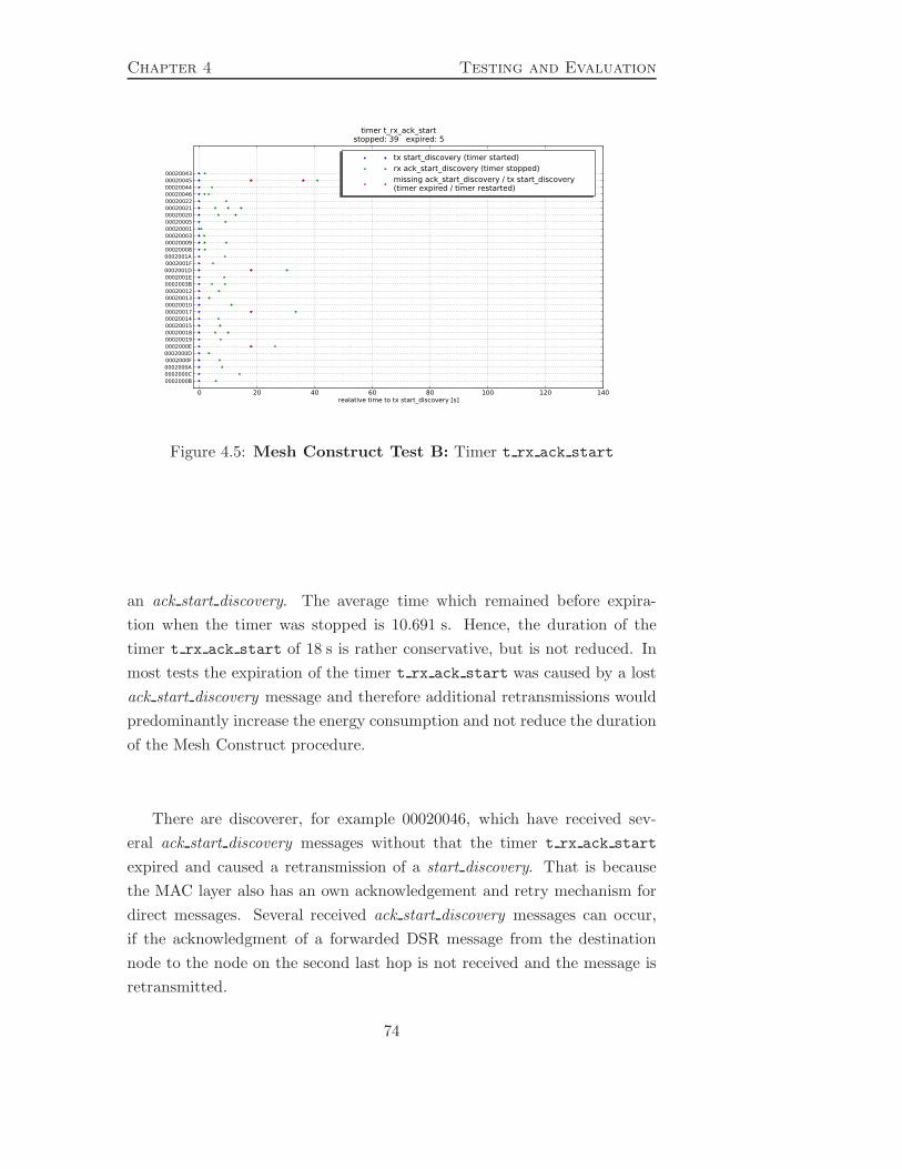
Chapter 4 Testing and Evaluation
0 20 40 60 80 100 120 140realative time to tx start_discovery [s]
0002000B0002000C0002000A0002000F0002000D0002000E00020019000200180002001500020014000200170002001000020013000200120002003B0002001E0002001D0002001F0002001A000200080002000900020003000200010002000500020020000200210002002200020046000200440002004500020043
timer t_rx_ack_startstopped: 39 expired: 5
tx start_discovery (timer started)rx ack_start_discovery (timer stopped)missing ack_start_discovery / tx start_discovery (timer expired / timer restarted)
Figure 4.5: Mesh Construct Test B: Timer t rx ack start
an ack start discovery. The average time which remained before expira-
tion when the timer was stopped is 10.691 s. Hence, the duration of the
timer t rx ack start of 18 s is rather conservative, but is not reduced. In
most tests the expiration of the timer t rx ack start was caused by a lost
ack start discovery message and therefore additional retransmissions would
predominantly increase the energy consumption and not reduce the duration
of the Mesh Construct procedure.
There are discoverer, for example 00020046, which have received sev-
eral ack start discovery messages without that the timer t rx ack start
expired and caused a retransmission of a start discovery. That is because
the MAC layer also has an own acknowledgement and retry mechanism for
direct messages. Several received ack start discovery messages can occur,
if the acknowledgment of a forwarded DSR message from the destination
node to the node on the second last hop is not received and the message is
retransmitted.
74

4.3 Timing Analysis Chapter 4
4.3.5 Timeout receive neighbor-table t rx nhtbl and requested
neighbor table t rq nhtbl
By setting the parameters of Table 4.2 into Equation 3.20 and 3.23 for the
duration of the timer t rx nhtbl and t rq nhtbl results
t rx nhtbl = 58.5 s · (1 + 1) + 6 s · (1 + 1) · (7 + 2) + 9 s (4.13)
= 288 s (4.14)
t rq nhtbl = 4 · 3 · 1.5 s (4.15)
= 18 s (4.16)
In Figure 4.6 the occuring events for all discoverers concerning the timers
t rx nhtbl and t rq nhtbl are plotted over the time relative to the start of
the timer t rx nhtbl. The timer t rx nhtbl starts with the transmission
of a start discovery and is stopped with the reception of a neighbor table.
When the timer t rx nhtbl expires a request nhtbl is transmitted and the
timer t rq nhtbl is started. When the timer t rq nhtbl expires another
request nhtbl is transmitted.
Most of the neighbor table messages are received much earlier as the
timer t rx nhtbl would expired. Therefore, to reduce the duration of the
Mesh Construct procedure in case of a lost neighbor table message the timer
t rx nhtbl is empirically set to 120 s. By this, the idle times of the dis-
coverers 0002001E, 0002003B, 00020018, and 0002000B are reduced about
three minutes each.
4.3.6 Maximal Duration of the Mesh Construct
By setting the parameters of Table 4.2 and the duration of the timers com-
puted in this section into Equation 3.29 for the maximal duration of the
Mesh Construct procedure t mc max results
t mc max = (32 − 1) ·
[(5 + 1) · 18 s + 120 s
+5 · 18 s + 9 s]
+120 s (4.17)
= 10257 s (4.18)
75
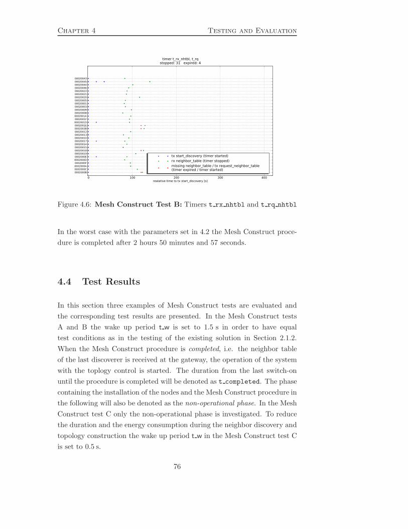
Chapter 4 Testing and Evaluation
0 100 200 300 400realative time to tx start_discovery [s]
0002000B0002000C0002000A0002000F0002000D0002000E00020019000200180002001500020014000200170002001000020013000200120002003B0002001E0002001D0002001F0002001A000200080002000900020003000200010002000500020020000200210002002200020046000200440002004500020043
timer t_rx_nhtbl, t_rqstopped: 31 expired: 4
tx start_discovery (timer started)rx neighbor_table (timer stopped)missing neighbor_table / tx request_neighbor_table (timer expired / timer started)
Figure 4.6: Mesh Construct Test B: Timers t rx nhtbl and t rq nhtbl
In the worst case with the parameters set in 4.2 the Mesh Construct proce-
dure is completed after 2 hours 50 minutes and 57 seconds.
4.4 Test Results
In this section three examples of Mesh Construct tests are evaluated and
the corresponding test results are presented. In the Mesh Construct tests
A and B the wake up period t w is set to 1.5 s in order to have equal
test conditions as in the testing of the existing solution in Section 2.1.2.
When the Mesh Construct procedure is completed, i.e. the neighbor table
of the last discoverer is received at the gateway, the operation of the system
with the toplogy control is started. The duration from the last switch-on
until the procedure is completed will be denoted as t completed. The phase
containing the installation of the nodes and the Mesh Construct procedure in
the following will also be denoted as the non-operational phase. In the Mesh
Construct test C only the non-operational phase is investigated. To reduce
the duration and the energy consumption during the neighbor discovery and
topology construction the wake up period t w in the Mesh Construct test C
is set to 0.5 s.
76

4.4 Test Results Chapter 4
4.4.1 Mesh Construct Test A
Duration
In Figure 4.7 the connectivity and hop count states of the Mesh Construct
Test A are plotted over the test time. In Figure 4.8 the same is plotted
over the non-operational phase containing the installation and the Mesh
Construct procedure. The Mesh Construct procedure is only started when
the last node is installed and powered on. After the last switch-on it takes 37
minutes and 35 seconds until the entire network is connected. The duration
t connected of the Mesh Construct test A clearly fulfills the requirement
to be less than one hour. The Mesh Construct procedure is completed after
52 minutes and 2 seconds.
Connectivity and Stability
After the network is connected, nb red nds is equal to zero for the entire
remaining test time. Therefore, all installed nodes are discovered.
After the network is connected and the Mesh Construct is completed
the operation starts and nb redyellow nds is equal to zero for the entire
remaining test time. Thus, the network remains connected during the oper-
ation.
In Figure 4.9 the number of dead neighbors, which are removed during
the test, is plotted over the test time. In total nb rem dead nhs = 1 dead
neighbors are removed during the test. In Figure 4.7 it can be observed that
the removal of one dead neighbor causes a connectivity state change at four
nodes from green+ to green. Since the mesh network topology constructed
by the Mesh Construct has a redundancy concerning the connectivity states,
the removal of one dead neighbor does not evoke yellow or red connectivity
states. During the test, except from a single dead neighbor removal, the
connectivity states are stable over the entire operation.
Energy Consumption
In Figure 4.10 the current consumtpion averaged over all targets is plotted
over the test time. The total consumed current of the Mesh Admin Test A is
divided into the five contributions I sleep, I carriersense, I overhear,
I rx, and I tx. I sleep is the current consumed in the energy-efficient sleep
state. I carriersense is the current required for the periodic wake up and
77

Chapter 4 Testing and Evaluation
0 2 4 6 8 10hours
0
10
20
30
40
50
num
ber
of
nodes
on c
onnect
ivit
y s
tate
green+greenyellow
redlast switch-onconnectedcompleted
0 2 4 6 8 10hours
0
10
20
30
40
50
num
ber
of
nodes
wit
h h
op c
ount
hc 0hc 1hc 2hc 3hc > 3last switch-onconnectedcompleted
Figure 4.7: Mesh Construct Test A: Upper plot: Number of nodes on
the corresponding connectivity states. Lower plot: Number of nodes on the
corresponding hop counts.
78
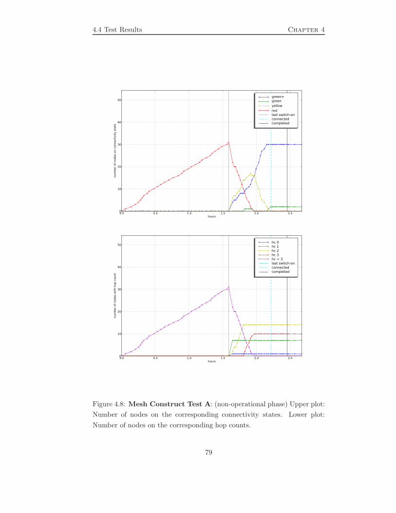
4.4 Test Results Chapter 4
0.0 0.5 1.0 1.5 2.0 2.5hours
0
10
20
30
40
50
num
ber
of
nodes
on c
onnect
ivit
y s
tate
green+greenyellow
redlast switch-onconnectedcompleted
0.0 0.5 1.0 1.5 2.0 2.5hours
0
10
20
30
40
50
num
ber
of
nodes
wit
h h
op c
ount
hc 0hc 1hc 2hc 3hc > 3last switch-onconnectedcompleted
Figure 4.8: Mesh Construct Test A: (non-operational phase) Upper plot:
Number of nodes on the corresponding connectivity states. Lower plot:
Number of nodes on the corresponding hop counts.
79

Chapter 4 Testing and Evaluation
0 2 4 6 8 10hours
0.0
0.2
0.4
0.6
0.8
1.0
tota
l dead n
eig
hbors
rem
oved
total dead neighbors removed
last switch-onconnectedcompleted
Figure 4.9: Mesh Construct Test A: Number of removed dead neighbors
of all nodes.
0 2 4 6 8 10 12time [h]
0
50
100
150
200
250
300
350
400
curr
ent
[uA
]
average current consumption of all targets:
I_sleep
I_carriersense
I_overhear
I_rx
I_tx
last switch-onconnectedcompleted
Figure 4.10: Mesh Construct Test A: The current consumption averaged
over all targets.
80

4.4 Test Results Chapter 4
carrier sense. I overhear is the current consumed for receiving messages
which originally are transmitted to a different destination. I rx, and I tx
are the currents consumed for receiving and transmitting messages.
The most energy is consumed during the Mesh Construct procedure,
in particular due to the transmissions of the energy expensive broadcasts.
The number of transmitted broadcasts is plotted in Figure 4.11 over the
test time. The total number of transmitted broadcasts nb tx bcasts dur-
ing the test is 96. Thus, each of the 32 nodes exactly transmitted the 3
scheduled broadcasts during the neighborhood discovery. No broadcasts are
transmitted during the operation.
0 2 4 6 8 10hours
0
20
40
60
80
100
tota
l tr
ansm
itte
d b
roadca
sts
total transmitted broadcastslast switch-onconnectedcompleted
Figure 4.11: Mesh Construct Test A: Number of transmitted broadcasts
of all nodes.
By comparing the time course of the current consumption with the time
course of the connectivity states in Figure 4.7, it can be observed, that the
current consumption is uniform during the operation if the network remains
connected.
In Figure 4.12 the current consumption of each individual detector aver-
aged over the entire test time is shown. Again, the current consumption is
divided into its five contributions. Overall, the current consumption of the
81

Chapter 4 Testing and Evaluation
0002000e
00020009
00020022
00020012
00020019
0002000d
0002000a
00020021
00020014
0002001d
00020015
00020017
0002003b
00020013
0002001e
00020008
00020043
0002000f
00020003
00020044
00020018
00020045
0002001f
0002000c
00020010
00020046
0002000b
0002001a
00020001
00020020
000200050
100
200
300
400
500cu
rrent
[uA
]
average current consumption of the targets after
I_sleepI_carriersenseI_overhearI_rxI_tx
Figure 4.12: Mesh Construct Test A: The average current consumption
of the nodes over the entire test time.
nodes is balanced. The total current consumption averaged over the time
and number of nodes i total is 89.328 µA.
4.4.2 Mesh Construct Test B
Duration
In Figure 4.13 the connectivity and hop count states of the Mesh Construct
Test B are plotted over the test time. In Figure 4.14 the same is plotted
over the non-operational phase containing the installation and the Mesh
Construct procedure. Again, the Mesh Construct procedure is only started
when the last node is installed and powered on. After the last switch-on
it takes 35 minutes and 50 seconds until the entire network is connected.
The duration t connected of the Mesh Construct test B clearly fulfills the
requirement to be less than one hour. The Mesh Construct procedure is
completed after 48 minutes and 47 seconds.
Connectivity and Stability
After the network is connected, nb red nds is equal to zero for the entire
remaining test time. Therefore, all installed nodes are discovered.
82

4.4 Test Results Chapter 4
0 2 4 6 8 10hours
0
10
20
30
40
50
num
ber
of
nodes
on c
onnect
ivit
y s
tate
green+greenyellow
redlast switch-onconnectedcompleted
0 2 4 6 8 10hours
0
10
20
30
40
50
num
ber
of
nodes
wit
h h
op c
ount
hc 0hc 1hc 2hc 3hc > 3last switch-onconnectedcompleted
Figure 4.13: Mesh Construct Test B: Upper plot: Number of nodes on
the corresponding connectivity states. Lower plot: Number of nodes on the
corresponding hop counts.
83

Chapter 4 Testing and Evaluation
0.0 0.5 1.0 1.5 2.0 2.5hours
0
10
20
30
40
50
num
ber
of
nodes
on c
onnect
ivit
y s
tate
green+greenyellow
redlast switch-onconnectedcompleted
0.0 0.5 1.0 1.5 2.0 2.5hours
0
10
20
30
40
50
num
ber
of
nodes
wit
h h
op c
ount
hc 0hc 1hc 2hc 3hc > 3last switch-onconnectedcompleted
Figure 4.14: Mesh Construct Test A: (non-operational phase) Upper
plot: Number of nodes on the corresponding connectivity states. Lower
plot: Number of nodes on the corresponding hop counts.
84

4.4 Test Results Chapter 4
0 2 4 6 8 10hours
�0.0010
�0.0005
0.0000
0.0005
0.0010
tota
l dead n
eig
hbors
rem
oved
total dead neighbors removed
last switch-onconnectedcompleted
Figure 4.15: Mesh Construct Test B: Number of removed dead neighbors
of all nodes.
85

Chapter 4 Testing and Evaluation
After the network is connected and the Mesh Construct is completed,
the operation starts and nb redyellow nds is equal to zero for the entire
remaining test time. Thus, the network remains connected during the oper-
ation.
In Figure 4.15 the number of dead neighbors, which are removed during
the test, is plotted over the test time. In total nb rem dead nhs = 0 dead
neighbors are removed during the test. In the Mesh Construct Test B the
connectivity states are constant and stable during the operation.
Energy Consumption
0 2 4 6 8 10 12 14time [h]
0
50
100
150
200
250
300
350
400
450
curr
ent
[uA
]
average current consumption of all targets:
I_sleep
I_carriersense
I_overhear
I_rx
I_tx
last switch-onconnectedcompleted
Figure 4.16: Mesh Construct Test B: The current consumption averaged
over all targets.
In Figure 4.16 the current consumtpion averaged over all targets is plot-
ted over the test time. Again, the total consumed current of the Mesh
Construct Test B is divided into the five contributions.
During the Mesh Construct procedure the most energy is consumed, in
particular due to the transmissions of the energy expensive broadcasts. The
number of transmitted broadcasts is plotted in Figure 4.17 over the test
time. The total number of transmitted broadcasts nb tx bcasts during the
test is 96. Thus, each of the 32 nodes exactly transmitted the 3 scheduled
broadcasts during neighborhood discovery. No broadcasts are transmitted
during the operation.
By comparing the time course of the current consumption with the time
86

4.4 Test Results Chapter 4
0 2 4 6 8 10hours
0
20
40
60
80
100
tota
l tr
ansm
itte
d b
roadca
sts
total transmitted broadcastslast switch-onconnectedcompleted
Figure 4.17: Mesh Construct Test B: Number of transmitted broadcasts
of all nodes.
00020022
0002000b
00020005
00020043
00020003
00020017
00020019
00020020
00020014
0002000f
0002000e
00020001
0002000a
0002001e
0002001f
00020044
00020018
00020010
00020013
0002001a
00020021
00020012
0002000d
00020046
0002003b
00020009
00020015
00020045
0002001d
00020008
0002000c0
100
200
300
400
500
curr
ent
[uA
]
average current consumption of the targets after
I_sleepI_carriersenseI_overhearI_rxI_tx
Figure 4.18: Mesh Construct Test B: The average current consumption
of the nodes over the entire test time.
87
Chapter 4 Testing and Evaluation
course of the connectivity states in Figure 4.7, it can be observed, that the
current consumption is uniform during the operation if the network remains
connected.
In Figure 4.18 the current consumption of each individual detector aver-
aged over the entire test time is shown. Again, the current consumption is
divided into its five contributions. Overall, the current consumption of the
nodes is balanced. The total current consumption averaged over the time
and number of nodes i total is 87.245 µA.
4.4.3 Mesh Construct Test C
The Mesh Construct procedure is initiated by a trigger mechanism at the
gateway and has a finite and determined duration after which the operation
is started. Therefore, it is theoretically possible to adjust paramteters at
the operation state changes, in particular when the neighbor discovery and
topology construction is started (The operation state changes from sleep to
discovery) and completed (The operation state changes from discovery to
operation).
The use of LPL in WSNs introduces a trade-off between energy-efficiency
and the latency, e.g. for transmissions of messages [13]. The shortening of
the wake up period on the one hand increases the wake up frequency and
hence the energy comsumption for carrier sensing but on the other hand,
increases the rate at which messages can be transmitted and additionally de-
creases the duration and thus the energy consumption of broadcasts. There-
fore, it is obvious that appropriately adapting the t w during the neighbor
discovery and topology control can reduce the duration and the energy con-
sumption of the Mesh Construct procedure.
Since the change of the parameter t w is not yet implemented in the
software, in the Mesh Construct Test C only the start up is investigated with
a t w set to 0.5 s. The operation and hence the stability of the procedure
are not considered.
Duration
In Figure 4.19 the connectivity and hop count states of the Mesh Construct
test C are plotted over the test time. After the last switch-on it takes 13
minutes and 5 seconds until the entire network is connected. The duration
t connected of the Mesh Construct test B clearly fulfills the requirement to
88
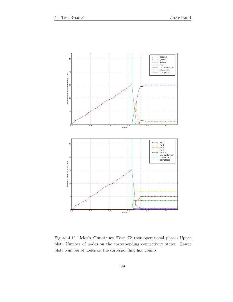
4.4 Test Results Chapter 4
0.0 0.5 1.0 1.5 2.0 2.5hours
0
10
20
30
40
50
num
ber
of
nodes
on c
onnect
ivit
y s
tate
green+greenyellow
redlast switch-onconnectedcompleted
0.0 0.5 1.0 1.5 2.0 2.5hours
0
10
20
30
40
50
num
ber
of
nodes
wit
h h
op c
ount
hc 0hc 1hc 2hc 3hc > 3last switch-onconnectedcompleted
Figure 4.19: Mesh Construct Test C: (non-operational phase) Upper
plot: Number of nodes on the corresponding connectivity states. Lower
plot: Number of nodes on the corresponding hop counts.
89
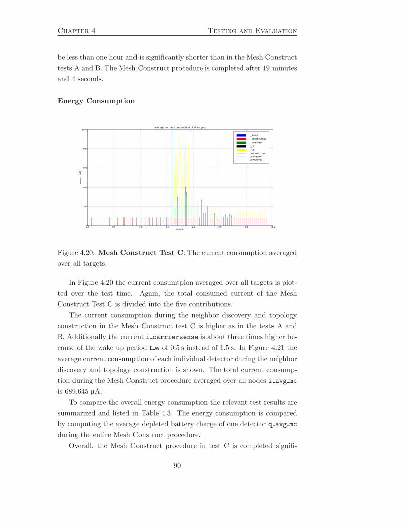
Chapter 4 Testing and Evaluation
be less than one hour and is significantly shorter than in the Mesh Construct
tests A and B. The Mesh Construct procedure is completed after 19 minutes
and 4 seconds.
Energy Consumption
0.0 0.5 1.0 1.5 2.0 2.5 3.0 3.5time [h]
0
200
400
600
800
1000
curr
ent
[uA
]
average current consumption of all targets:
I_sleep
I_carriersense
I_overhear
I_rx
I_tx
last switch-onconnectedcompleted
Figure 4.20: Mesh Construct Test C: The current consumption averaged
over all targets.
In Figure 4.20 the current consumtpion averaged over all targets is plot-
ted over the test time. Again, the total consumed current of the Mesh
Construct Test C is divided into the five contributions.
The current consumption during the neighbor discovery and topology
construction in the Mesh Construct test C is higher as in the tests A and
B. Additionally the current i carriersense is about three times higher be-
cause of the wake up period t w of 0.5 s instead of 1.5 s. In Figure 4.21 the
average current consumption of each individual detector during the neighbor
discovery and topology construction is shown. The total current consump-
tion during the Mesh Construct procedure averaged over all nodes i avg mc
is 689.645 µA.
To compare the overall energy consumption the relevant test results are
summarized and listed in Table 4.3. The energy consumption is compared
by computing the average depleted battery charge of one detector q avg mc
during the entire Mesh Construct procedure.
Overall, the Mesh Construct procedure in test C is completed signifi-
90

4.4 Test Results Chapter 4
00020017
00020044
0002003b
0002000c
00020008
00020009
00020015
00020012
00020013
00020001
00020045
00020021
0002001f
0002000a
00020019
0002001d
0002000e
00020043
00020005
0002000d
0002001e
0002000b
00020022
00020014
00020010
00020003
0002001a
0002000f
00020020
00020018
000200460
100
200
300
400
500
600
700
800
900
curr
ent
[uA
]
average current consumption of the targets after
I_sleepI_carriersenseI_overhearI_rxI_tx
Figure 4.21: Mesh Construct Test C: The average current consumption
of the nodes during the Mesh Construct procedure.
Test A Test B Test C
t completed 3122 s 2927 s 1144 s
i avg mc 295.830 µA 291.390 µA 689.645 µA
q avg mc 0.924 As 0.853 As 0.789 As
Table 4.3: Energy consumption during the Mesh Construct procedure
91

Chapter 4 Testing and Evaluation
cantly faster than in Test A and B and less energy is consumed as assessed
by the depletion of the battery charge.
4.5 Comparison with the Existing Solution
In this section the test results of the Mesh Construct tests are compared
to the test results obtained with the existing solution. The values of the
defined quality metrics are summarized and listed in Table 4.4.
eS test A eS test B MC test A MC test B
t connected 1 h 17 min 47 s 17 min 22 s 37 min 35 s 35 min 50 s
max(nb red nds) * 0 0 0 0
max(nb redyellow nds) * 4 2 0 0
nb rem dead nhs 104 89 1 0
nb tx bcasts 37 36 96 96
i total 144.090 µA 123.536 µA 89.328 µA 87.245 µA
Table 4.4: Comparison between the existing Solution (eS) and the Mesh
Construct (MC). (*: The maximal value after the network is connected the
first time until the test end is considered.)
In general, the results of the Mesh Construct test are more homogeneous
than the results of the existing solution, especially the duration t connect.
It can be assumed that, the heterogeneous nature of the results obtained
with the existing solution arises from the fact that the existing solution is a
random procedure, whereas the Mesh Construct is deterministic. In partic-
ular, depending on the random order of the node switch-ons a completely
different network topology is constructed with the existing solution. For ex-
ample this can be observed by comparing the different compositions of the
hop counts in the Figures 2.1 and 2.1. In the Mesh Construct tests, indepen-
dent of the random order of the switch-ons, exactly the same composition
of hop counts can be observed after the network is connected.
Duration
In constrast to the existing solution, in each Mesh Construct test the du-
ration t connect is less than one hour. However, there are test examples,
where the existing solution is connected faster than the Mesh Construct.
Connectivity and Stability
With both, the Mesh Construct or the existing solution all nodes are discov-
92

4.5 Comparison with the Existing Solution Chapter 4
ered. During the operation the network constructed by the existing solution
attains several times a yellow network connectivity state whereas with the
Mesh Construct the network remains connected. By considering the plots
of the connectivity states and the number of removed dead neighbors, the
Mesh Construct procedure results in a more stable network topology than
the existing solution.
Energy Consumption
Although the number of transmitted broadcasts of the Mesh Construct is
sharply higher, the overall average current consumption per node is lower
than in the existing solution. That is because energy can be saved by a
stable network topology in terms of connectivity.
93

Chapter 5 Conclusions
Chapter 5
Conclusions
In the first section of this chapter the work presented in this thesis is sum-
marized. The achieved contributions are indicated in the second section. In
the last section an outlook on possible future work in the area of this thesis
is given.
5.1 Summary
In this thesis the new procedure Mesh Construct for the neighbor discovery
and topology construction of a multihop WSN is presented. The objective
of the procedure is to be fast and energy-efficient. In addition, a stable and
constant mesh network topology with certain characteristics for the purpose
of the operational phase of the WSN shall be constructed.
A fire alarm system based on a multihop WSN is the underlying system
investigated in this thesis. Due to the safety-critical function of a fire alarm
system a mesh network topology with at least two node-disjoint multihop
communication paths from each detector to the gateway is required to ensure
reliable alarm forwarding in case of detector failures. A network connectivity
state is defined in order to indicate whether the mesh network topology
fulfills this requirement.
The Mesh Construct procedure is controlled by the gateway and con-
structs the mesh network topology through initiating sequentially neighor-
hood discoveries on each discovered node starting from the gateway and
proceeding outwards hop by hop. Nodes performing a neighborhood dis-
covery choose the best discovered nodes for the purpose of the network as
neighbors. In case of the fire alarm system, neighbors which can improve
94

5.1 Summary Chapter 5
the network connectivity state and have a good link quality are prefered.
After the neighborhood discovery, the choice is stored in a neighbor table
and transmitted to the gateway, which maintains and updates the network
informations in order to be able to initiate the next neighborhood discov-
eries. The Mesh Construct is completed when the neighbor table of each
discoverer is received at the gateway and the operation of the WSN including
a topology control can be started.
Tests and evaluations of the existing solution for the network initializa-
tion and topology control revealed several results: First, there is no finite
deterministic upper bound for the duration of the network initialization.
Second, during the operation the mesh network topology is unstable and
sometimes the required network connectivity state is not ensured, due to re-
movals of inappropriate neighbors by the topology control. Third, the neigh-
bor removals cause unconnected nodes to discover new neighbors, which
significantly increases the energy consumption.
Through the insights gained from the evaluation of the existing solution
the choice of the neighbors during the neighborhood discovery and the hop
by hop construction of the mesh network topology are crucial elements in
the conceptual design of the Mesh Construct to improve the performance of
the neighbor discovery and topology construction.
Although the amount of performed Mesh Construct tests is not staticsti-
cal relevant, the examples of test evaluations show promising results. First,
the duration of the Mesh Construct procedure is finite and fast enough to
fulfill the requirements. Second, the appropriate choice of neighbors and the
hop by hop construction reduce neighbor removals during the operation and
lead to a more stable and better connected mesh network topology com-
pared to the tests with the existing solution. Third, through the stable and
connected network topology the total energy consumption during the tests
is reduced compared to the tests with the existing solution.
Moreover, the triggered start and the finite duration of the procedure
allow to adjust parameters at operation state changes. A Mesh Construct
test with a shorter wake up time period of the WiseMAC, showed that the
duration and the energy consumption can be further reduced during the
neighbor discovery and topology construction.
95
Chapter 5 Conclusions
5.2 Contributions
In the following the main achievements and contributions of this thesis are
stated.
• The presented Mesh Construct is a procedure with the objective to
discover neighbors and construct a stable and connected mesh network
toplogy in a fast and energy-efficient way. In particular, the Mesh
Construct is suited for an alarm system based on a multihop WSN.
• The Mesh Construct procedure has a triggered start and a finite dura-
tion. A deterministic upper bound for the duration can be computed.
The triggered start and finite duration theoretically allow to appro-
priately adjust parameters for the different operation states, before,
during and after the Mesh Construct prodecure.
• With appropriate parameter choices the possiblity to rate and choose
neighbors depending on the link quality or the resulting connectivity
state improvement is provided. For an alarm system a good choice
can decrease the instability and introduce redundancy on the network
connectivity state in order to prevent the network from getting uncon-
nected in case of limited neighbor removals by the topology control
during operation.
• With the informations about the network topology at the gateway,
installed nodes which are not discovered can be identified and possibly
placed in an more appropriate location for the network.
• The Mesh Construct applied to the fire alarm system described in
Section 1.1.2 can reduce energy consumption, duration, and instability
in the mesh network topology.
5.3 Outlook
In this section proposals for possible future work in the area of this thesis
are indicated:
• To achieve a statistical relevance of the evaluation results more tests
in series could be performed and evaluated.
96

5.3 Outlook Chapter 5
• By running more tests with systematic choices of all the possible pa-
rameter constellations the performance of the Mesh Construct for a
particular application could be optimized.
• The possiblity of the Mesh Construct to adapt parameters at oper-
ation state changes could be implemented in practice to improve the
performance during the neighbor discovery and topology construction.
For example, as showed with the Mesh Construct test C, the energy
consumption and the duration of the Mesh Construct procedure can
be decreased by shortening the WiseMAC wake up period t w. In ad-
dition, a longer t w could reduce the energy consumed for the periodic
carrier sense in the operation state before the Mesh Construct actually
is started.
97

Appendix A Testbed
Appendix A
Testbed
In this section of the appendix the testbed used in the tests documented in
Section 2.1.2 and Chapter 4 is described. Several parts of the testbed were
developed during the master’s thesis of Florian Betschart [14].
The testbed consists of 32 nodes, which can be used either for the gate-
way or for the detectors. The radio module on the nodes is based on a
MSP430 microprocessor [15] and uses an ADF7021 low power narrow-band
transceiver for wireless communication in the sub-gigahertz frequency band.
The MSP430 has 4 kilobytes random access memory (RAM) and 56 kilobytes
read only memory (ROM).
A Deployment Support Network (DSN) [16] is applied to the nodes of
the testbed. The DSN is a second network laid out above the actual WSN in
order to monitor, configure and reprogram the sensor nodes using a remote
procedure call protocol. The DSN applied to the testbed is based on a hybrid
solution of USB-interfaced DSN nodes and an Ethernet platform. Each
sensor node is attached to an adapterboard equipped with an USB-interface.
The adaptorboards are connected via USB to an Ethernet gateway, which
uses a TCP/IP stack to communicate with a DSN-server. The DSN-server
provides an interface to access the DSN and initiate several different tasks,
which can be accomplished through the DSN:
• New compiled software code can be downloaded to the microprocessor
of the sensor nodes.
• Sensor nodes can be enabled and disabled.
• Tests can be started.
98

Testbed Appendix
• Debug, warn, and error logs of the nodes can be read out.
• Collected statistics of the sensor nodes can be read out.
The read out statistics during tests are directly stored in a MySQL
database [17]. Over the logs of the nodes and the MySQL database test
results can be evaluated and analyzed.
99

Appendix BIBLIOGRAPHY
Bibliography
[1] International Frequency Management: International Telecommunica-
tion Union, http://www.itu.int/itu-r/terrestrial/faq/index.html, Okto-
ber 2009.
[2] JasonL. Hill and DavidE. Culler. Mica: A wireless platform for deeply
embedded networks. IEEE Micro, 22(6):12–24, 2002.
[3] A. El-Hoiydi and J. D. Decotignie. Wisemac: an ultra low power mac
protocol for the downlink of infrastructure wireless sensor networks.
volume 1, pages 244–251 Vol.1, 2004.
[4] Mario Strasser, Andreas Meier, Koen Langendoen, and Philipp Blum.
Dwarf: Delay-aware robust forwarding for energy-constrained wireless
sensor networks. In Proceedings of the 3rd IEEE International Con-
ference on Distributed Computing in Sensor Systems (DCOSS 2007),
pages 64–81, June 2007.
[5] DIN VDE 0833-2: Gefahrenmeldeanlagen fur Brand, Einbruch und
Uberfall Teil 2: Festlegungen fur Brandmeldeanlagen (BMA), Februar
2004.
[6] Andreas Meier, Matthias Woehrle, Mischa Weise, Jan Beutel, and
Lothar Thiele. Nose: Efficient maintenance and initialization of wireless
sensor networks. In Proc. Sixth Annual IEEE Communications Society
Conference on Sensor, Mesh, and Ad Hoc Communications and Net-
works (SECON 2009), pages 1–9, Rome, Italy, June 2009. IEEE.
[7] Andreas Meier, Mischa Weise, Jan Beutel, and Lothar Thiele. Poster
abstract: NoSE: Neighbor search and link estimation for a fast and
energy efficient initialization of wsns. In Proc. 6th ACM Conf. Embed-
100
BIBLIOGRAPHY Appendix
ded Networked Sensor Systems (SenSys 2008), pages 397–398, Raleigh,
North Carolina, USA, November 2008. ACM.
[8] Michael J. Mcglynn and Steven A. Borbash. Birthday protocols for low
energy deployment and flexible neighbor discovery in ad hoc wireless
networks. In MobiHoc ’01: Proceedings of the 2nd ACM international
symposium on Mobile ad hoc networking & computing, pages 137–
145, New York, NY, USA, 2001. ACM.
[9] Roger Wattenhofer and Aaron Zollinger. XTC: A Practical Topology
Control Algorithm for Ad-Hoc Networks. In 4th International Work-
shop on Algorithms for Wireless, Mobile, Ad Hoc and Sensor Networks
(WMAN), Santa Fe, New Mexico, April 2004.
[10] D.Angelosante, E.Biglieri, and M.Lops. A simple algorithm for neigh-
bor discovery in wireless networks. In Acoustics, Speech and Signal
Processing, 2007. ICASSP 2007. IEEE International Conference on,
volume 3, pages III–169–III–172, 2007.
[11] Andreas Meier, Tobias Rein, Jan Beutel, and Lothar Thiele. Coping
with unreliable channels: Efficient link estimation for low-power wire-
less sensor networks. In Proc. 5th Intl Conf. Networked Sensing Systems
(INSS 2008), pages 19–26, Kanazawa, Japan, June 2008. IEEE.
[12] Kannan Srinivasan and Philip Levis. RSSI is under appreciated. In
Proc. 3rd Workshop on Embedded Networked Sensors (EmNets 2006),
May 2006.
[13] Thomas Moscibroda, Pascal von Rickenbach, and Roger Wattenhofer.
Analyzing the energy-latency trade-off during the deployment of sensor
networks. In 25th Annual Joint Conference of the IEEE Computer and
Communications Societies (INFOCOM), Barcelona, Spain, April 2006.
[14] Betschart Florain. Ethernet-based deployment support network. Mas-
ter’s thesis, Swiss Federal Institute of Technology, Zurich, Switzerland,
2008. Under the supervision of Prof. Dr. Lothar Thiele.
[15] Texas Instruments, Microcontroller MSP430, http://focus.ti.com/mcu/
docs/mcuprodoverview.tsp?sectionid=95&tabid=140&familyid=342,
Oktober 2009.
101

Appendix BIBLIOGRAPHY
[16] Matthias Dyer, Jan Beutel, Lothar Thiele, Thomas Kalt, Patrice Oe-
hen, Kevin Martin, and Philipp Blum. Deployment support network
- a toolkit for the development of wsns. In Proc. 4th European Conf.
on Wireless Sensor Networks (EWSN 2007), pages 195–211. Springer,
Berlin, January 2007.
[17] Sun Microsystems, MySQL database, www.mysql.com, Oktober 2009.
102