MASTER THESIS - MOnAMi | MOnAMi - Publication … function candidate and showing negative...
41
MASTER THESIS Herr Grigory Devadze Analysis of control system stability under algorithmic uncertainty 2016
-
Upload
trinhkhanh -
Category
Documents
-
view
218 -
download
0
Transcript of MASTER THESIS - MOnAMi | MOnAMi - Publication … function candidate and showing negative...

MASTER THESIS
HerrGrigory Devadze
Analysis of control systemstability under algorithmic
uncertainty
2016


Fakultät Angewandte Computer- undBiowissenschaften
MASTER THESIS
Analysis of control systemstability under algorithmic
uncertainty
Autor:Grigory Devadze
Studiengang:Applied Mathematics in Digital Media
Seminargruppe:MA14w1
Erstprüfer:Prof. Dr.-Ing. Alexander Lampe
Zweitprüfer:Dr.-Ing. Pavel Osinenko
Mittweida, Dezember 2016


Bibliografische Angaben
Devadze, Grigory: Analysis of control system stability under algorithmic uncertainty, 29 Seiten,5 Abbildungen, Hochschule Mittweida, University of Applied Sciences, Fakultät AngewandteComputer- und Biowissenschaften
Master Thesis, 2016
Dieses Werk ist urheberrechtlich geschützt.
Referat
Stability of control systems is one of the central subjects in control theory. The classical asymp-totic stability theorem states that the norm of the residual between the state trajectory and theequilibrium is zero in limit. Unfortunately, it does not in general allow computing a concrete rateof convergence particularly due to algorithmic uncertainty which is related to numerical imper-fections of floating-point arithmetic. This work proposes to revisit the asymptotic stability theorywith the aim of computation of convergence rates using constructive analysis which is a math-ematical tool that realizes equivalence between certain theorems and computation algorithms.Consequently, it also offers a framework which allows controlling numerical imperfections in acoherent and formal way. The overall goal of the current study also matches with the trend ofintroducing formal verification tools into the control theory. Besides existing approaches, con-structive analysis, suggested within this work, can also be considered for formal verification ofcontrol systems. A computational example is provided that demonstrates extraction of a conver-gence certificate for example dynamical systems.


I
I. Contents
Contents . . . . . . . . . . . . . . . . . . . . . . . . . . . . . . . . . . . . . . . . . . . . . . . . . . . . . . . . . . . . . . . . . . . . . . . . . . . . . . . . . . . . . . . . . . I
List of Figures . . . . . . . . . . . . . . . . . . . . . . . . . . . . . . . . . . . . . . . . . . . . . . . . . . . . . . . . . . . . . . . . . . . . . . . . . . . . . . . . . . . . . II
Preface . . . . . . . . . . . . . . . . . . . . . . . . . . . . . . . . . . . . . . . . . . . . . . . . . . . . . . . . . . . . . . . . . . . . . . . . . . . . . . . . . . . . . . . . . . . . III
1 Introduction . . . . . . . . . . . . . . . . . . . . . . . . . . . . . . . . . . . . . . . . . . . . . . . . . . . . . . . . . . . . . . . . . . . . . . . . . . . . . . . . . . . 1
1.1 Problem Statement . . . . . . . . . . . . . . . . . . . . . . . . . . . . . . . . . . . . . . . . . . . . . . . . . . . . . . . . . . . . . . . . . . . . . . . . . . 1
1.2 Selected approaches to formal verification of control systems . . . . . . . . . . . . . . . . . . . . . . . . . . . . 2
2 Mathematical frameworks for formal stability analysis . . . . . . . . . . . . . . . . . . . . . . . . . . . . . . . . . . . . . 5
2.1 Brief overview of constructive analysis and selected notions . . . . . . . . . . . . . . . . . . . . . . . . . . . . . . 6
2.2 Brief overview of Lyapunov stability theory . . . . . . . . . . . . . . . . . . . . . . . . . . . . . . . . . . . . . . . . . . . . . . . . . 12
2.3 Constructive stability analysis . . . . . . . . . . . . . . . . . . . . . . . . . . . . . . . . . . . . . . . . . . . . . . . . . . . . . . . . . . . . . . . 14
2.4 Algorithmic realization . . . . . . . . . . . . . . . . . . . . . . . . . . . . . . . . . . . . . . . . . . . . . . . . . . . . . . . . . . . . . . . . . . . . . . . 18
2.5 Case study and discussion . . . . . . . . . . . . . . . . . . . . . . . . . . . . . . . . . . . . . . . . . . . . . . . . . . . . . . . . . . . . . . . . . . 20
3 Conclusion . . . . . . . . . . . . . . . . . . . . . . . . . . . . . . . . . . . . . . . . . . . . . . . . . . . . . . . . . . . . . . . . . . . . . . . . . . . . . . . . . . . 23

II
II. List of Figures
2.1 Consistency of BISH with CLASS, INT and RUSS. [1] . . . . . . . . . . . . . . . . . . . . . . . . . . . . . . . . . . . . 7
2.2 Function w3 – upper bound on the derivative of the Lyapunov function . . . . . . . . . . . . . . . . . . . 20
2.3 Convergence certificate and example system trajectories . . . . . . . . . . . . . . . . . . . . . . . . . . . . . . . . . 21
2.4 Three-dimensional illustration of the convergence certificate and example system tra-
jectories . . . . . . . . . . . . . . . . . . . . . . . . . . . . . . . . . . . . . . . . . . . . . . . . . . . . . . . . . . . . . . . . . . . . . . . . . . . . . . . . . . . . . . 21
2.5 Levels sets of the convergence certificate and example system trajectories . . . . . . . . . . . . . 22


III
III. Preface
Algorithmic uncertainty within the current work is understood as discrepancy betweenidealized mathematical algorithms and their numerical realizations. Algorithmic uncer-tainty may result, for example, from discretization and numerical approximation. Infloating-point approximations, unexpected errors due to roundoff may occur. In con-trast to the floating-point arithmetic, there exist so-called exact real number arithmetics,some of which use algorithmic representation of real numbers which potentially allowarbitrarily approximation of the given real number. Exact real number arithmetic is oftenused in automated theorem proving software [2–6]. An example of an automated andformalized proof is the proof of Kepler’s conjecture [7]. The present thesis is focused onthe issues of algorithmic uncertainty with regards to system stability.
System stability has been among the most crucial subjects of control theory. Tradi-tionally, stability of control systems is analyzed within the Lyapunov theory [8] first intro-duced in 1892. The Lyapunov function method (also called second method of Lyapunov)lies in the heart of numerous controller designs found in literature. To certain extent, itgeneralizes the concept of mechanical energy to abstract systems. Dealing with thenumerical uncertainty in connection with the proving of stability properties is a certaindifficulty. Heuristics and post-processing are often required to quantify and to eliminatethe uncertainties. Depending on the application’s goal, numerical methods sometimeshave to be adapted in order to fulfill requirements on the accuracy and robustness.
There is a relatively new but important framework, the so-called formal verification, thatwas suggested to address formal correctness of software and systems. Formal verifica-tion, i. e., verification of system’s properties within some formal logical system, recentlystarted attracting much attention of the control engineering community [9–16]. Formalcorrectness may be seen as a formal certificate ensuring that the behavior of the systemmatches with the designed one for the whole space of possible input conditions. As forthe stability theory, it means providing a formal certificate, i. e., a certain mathematicalconstruct, that assures boundedness or convergence of the system trajectories to theequilibrium. Incorrect functioning may drive the behavior away from the expected one.Consequences of failures may be as bad as damage to the devices and human health,not just deteriorated performance. In investigation of correctness of system’s stability,one may be interested in answering the following questions: “What is a bound on themagnitude of a system trajectory starting from so or so initial condition?”, “How fastdoes the trajectory converge to the equilibrium?”. The classical Lyapunov theory doesnot in general provide answers to these questions. For example, finding an appropriateLyapunov function candidate and showing negative definiteness of its time derivativeensures “energy decay” in the system and, consequently, convergence. However, thetheory in general does not provide a rate of convergence. Even though it shows that the

III
limit of the metric between the system trajectory and the equilibrium is zero as time goesto infinity, it does not say how fast the said metric decays. It is so due to the classicaldefinition of a limit. The definition merely states what the “value at infinity” is, but doesnot provide any information on the rate of convergence. To deal with this problem, theconcept of exponential stability is sometimes used instead, but it is harder to verify thanasymptotic stability. Perhaps, using a different notion of a limit, which would necessarily“encode” a rate of convergence and address algorithmic uncertainty, might provide apractically useful framework for formal verification of control system stability. This is thecentral question of the current study. In other words, what is necessary information tobe provided within a Lyapunov function that allows “computing” the rate of convergenceof the state trajectories up to any given precision thus having algorithmic uncertaintyunder control?

Chapter 1: Introduction 1
1 Introduction
1.1 Problem Statement
The current work proposes to revisit the control system stability theory with the aim ofconvergence rates under algorithmic uncertainty. The key ingredient of the proposalis the constructive analysis which is a mathematical tool that realizes equivalence be-tween certain theorems and computation algorithms. The classical asymptotic stabilitytheorem merely states that the norm of the residual between the state trajectory and theequilibrium is zero in limit. It does not in general allow computing the concrete rate ofconvergence. The stability theorem is revisited constructively which allows computingthe convergence rates, also called convergence certificates in the current framework.The result requires, however, certain additional conditions on the Lyapunov function.Nevertheless, these conditions can be met in practice without a large extra design ef-fort. The overall goal of the current study matches with the trend for introducing formalverification tools into the control theory. It is suggested that the constructive analysismight serve as one of the good starting points to this end. The computational exampleis provided that demonstrates extraction of a convergence certificate for a sample dy-namical system. A formal stability certificate is, within the current study, a function oftime, which may in general depend on the initial condition, which puts an upper boundon the metric between the system trajectory and the equilibrium.
The current work starts with a review of selected existing approaches to formal verifi-cation of control systems in Section 1.2 followed by a brief description of mathematicalframeworks which may help address the stated problem (Section 2). In particular, abrief history and selected notions of constructive analysis, which is in the focus of thecurrent work, are presented, in Section 2.1. A brief review of Lyapunov stability theoryis given in Section 2.2. Section 2.3 is concerned with analysis of asymptotic stabilitywith the goal of computing formal certificates of asymptotic stability whereas Section2.4 presents a concrete algorithmic realization. Section 2.5 presents case studies.
2 Chapter 1: Introduction
1.2 Selected approaches to formal verification ofcontrol systems
Formal verification methods have been attracting attention of the control engineeringcommunity in the recent years and the proposed approaches are diverse. To demon-strate this, some selected ones are briefly reviewed in this section. They can be trackedto as early as the work of Livadas [17] where he addressed formal verification for col-lision avoidance in hybrid systems. The major apparatus used was hybrid input-outputautomata. The work suggested a special abstract notion – called protector – to guaran-tee compliance with safety requirement. Correctness proof of the protector was estab-lished within the theory of hybrid input-output automata. Similar issues were addressedby Franzle [18] where he investigated formal logics of hybrid automata and the relatedreachability issues. Later, Mysore et al. [19] applied formal logic of hybrid automatato systems biology. An important property of these two formal logic approaches wasquantifier elimination, i. e., deriving formally true quantifier-free logical formulas.
In their project dedicated to formal verification methods to the European Train ControlSystem (ETCS), Platzer et al. [20] also suggested to use quantifier elimination. Thebackground formal system was differential dynamic logic.This is a first-order system forformalization of hybrid systems which can be generalized to formalize also differentialequations. The ETCS was formalized and verified within the differential dynamic logicthroughout an iterative process including the so-called controllability discovery, controlrefinement, safety convergence and liveness check steps. A more generalized and sub-stantial description of the framework of differential dynamic logic applied to dynamicalsystems with an extensive set of examples was given in [9]. It is important to noticetheir background number field – the real closed field – that enables quantifier elimina-tion [21]. Another firm application of differential dynamic logic can be found in Looset al. [22] where they addressed safety of distributed aircraft systems. The works byPlatzer et al. also offer a good literature review on the subject matter for an interestedreader. Hybrid Hoare logic was used by Zou et al. [23] to formally verify a control sys-tem within the Chinese train network. They claimed to better address parallelism andcommunication issues within their approach than the one based on differential dynamiclogic.
Automated theorem proving – performed by special software called proof assistants– also plays an important role in formal verification of control systems. For instance,Platzer et al. [24] developed automated theorem proving methods within their differ-ential dynamic logic. Description of their software tool – KeYmaera – cay be foundin [25]. Zou et al. [23] used Isabelle for implementation of their control system for-mal verification based on Hybrid Hoare logic. A tool called Why3 coupled with MAT-LAB/Simulink was used in more recent works by Araiza et al. [10,26] to perform simplestability checks of linear discrete systems with quadratic Lyapunov functions. Their

Chapter 1: Introduction 3
method may be considered complimentary to the available model verifiers availablewithin MATLAB/Simulink. [13] mentioned several automated theorem proving softwaretools to be considered for implementation of formal verification of control systems –Coq, HOL Light, Isabelle, Lean. His work also indicated the importance of the questionraised within the current study. He suggested to address formal analysis of the theo-ries like stability, including Lyapunov theory, observability, controllability, optimal, robust,and adaptive control. As a logical frameworks for computations, he suggested to usethe Type Two Theory of Effectivity developed by Weihrauch (see, for example, [27–29]).This theory will be briefly reviewed in Section 2. Gao [13] also reviewed a solver calleddReal for solving logical formulas in nonlinear dynamical systems theory. Siddique etal. [15] used HOL Light in their formalization of photonic systems. Among other aspects,they formalized difference equations and z-transform within the proof assistant. A re-cent work by Bernardeschi et al. [30] proposed to use the Prototype Verification Systemas the proof assistant for verification of a water level controller. Formalization of thebehavior and safety requirement verification were carried out. The Munich project onformal verification of cyber-physical systems is another representative example. Withinit, Althoff et al. [11, 12] extensively used reachability analysis with zonotopes for ver-ification of power system stability and automated road vehicles respectively. Kong etal. [14] investigated applications of reachable sets to semi-algebraic dynamical systemswith polynomial approximators of sets in Euclidean space as their central concept. Theyfocused on inductive invariants which are certain properties of dynamical systems thathold from the initial state throughout the system trajectories. Chan et al. [16] recentlyalso addressed formal verification of cyber-physical systems using Coq proof assistant.In their work, they addressed formal verification within the Lyapunov stability theory.
An ongoing European research project on formal verification of stability of embeddedcontrol systems (see description under cordis.europa.eu/project/rcn/
/187016_en.html) is dedicated to algorithmic methods of correctness check andalso demonstrates the importance of the questions raised within the current study.
To summarize, the given review clearly indicates that application of different formal me-thods has certain merits for control theory, especially regarding tackling algorithmic un-certainty. The software tools and logical foundations are diverse. However, a certain ef-fort is required for a control systems engineer to start working with the mentioned tech-niques since they are loaded with background in pure logic that is not usually largelyrepresented within engineering education. This also concerns the Weihrauch’s com-putable analysis suggested as the major framework by Gao [13]. In the next section, abrief description of computable analysis is provided. On the other hand, the next sectionalso proposes another background mathematical foundation for formal analysis of con-trol systems under algorithmic uncertainty – constructive analysis – and it will be shownsuch an approach might have a certain merit. It is believed that constructive analysismight better match with the mathematical education a control engineer usually receives.The details are given in the second part of the next section.

4

Chapter 2: Mathematical frameworks for formal stability analysis 5
2 Mathematical frameworks for formalstability analysis
As was seen in the previous section, mathematical frameworks and logical systems forformal verification of control systems are diverse. Some of them, such as differential dy-namic logic, might require certain background in formal logic to start using this approach.In this section, however, the focus is set on the Weihrauch’s computable analysis andconstructive analysis as developed by Bishop [31]. The Weihrauch’s computable anal-ysis has a notion of a computable mathematical object as the central concept. “Com-putable” in this context means effectively computable. That is, an algorithm computingthe mathematical object in question must consist only of finitely many exact instruc-tions, it needs to always terminate and produce a correct answer. The Weihrauch’scomputable analysis formalizes this concept and defines precisely what computablenumbers, computable functions and other computable objects are. It relies on the no-tion of a Turing machine – an abstract device performs certain actions on a strip of tape– first formalized by Turing [32]. The real numbers are represented as infinite binarysequences produced by Turing machines. A function on real numbers is in turn calledcomputable whenever there is a Turing machine which computes each infinite binarysequence representing a real number into some sequence representing the value of thefunction.
Roughly speaking, the Weihrauch’s computable analysis mostly works with the saidrepresentations and shows that so or so mapping is computable. Even though, such aframework attracted some attention in the control engineering community, two subtletiesneed to be indicated. First, the background logic of the Type Two Theory of Effectivityis classical. Without going into detail so far, it means the following: the computationsmerely need to terminate, but there is no way to calculate the bound on the maximumnumber of iterations after which the computation finishes. This idea can be illustratedon the example of BlooP and FlooP programming languages introduced by Hofstadter[33] to illustrate certain logical derivations. Essentially, BlooP is a simple programminglanguages that allows only bounded loops – the “for ... do” loop. On contrary, FlooPallows unbounded loops such as “while ... do” loops. Unlike FlooP, BlooP is not Turing-complete in that one cannot program every computable function in it.
Another subtlety is the framework of the Weihrauch’s computable analysis itself whichis heavily formal and might be unusual for an engineer. Instead of numbers and func-tions, there are representations and Turing machines. Perhaps, it may be appropriate forcertain formal verification problems, but the current study is concerned with mathemat-ical framework for adressing algorithmic uncertainty and formal analysis – constructiveanalysis – which is briefly described further.

6 Chapter 2: Mathematical frameworks for formal stability analysis
2.1 Brief overview of constructive analysis andselected notions
The history of constructive analysis began in 1907. The Dutch mathematician Brouwercriticized in his doctoral thesis several concepts of classical mathematics (further de-noted by CLASS) and suggested the so-called intuitionistic mathematics (INT) as analternative [34].
One of its interpretations is due to Brouwer, Heyting and Kolmogorov (sometimes calledBHK interpretation or realizability interpretation) which states the fundamental logicalrules for what can be interpreted as a mathematical proof [35]. Let P and Q be somearbitrary formulas. One of the most important rules in BHK are:
1. Proving the implication P⇒Q means finding an algorithm that transforms a proofof P into a proof of Q
2. To prove ∃a.P[a], an algorithm computing a and the proof that P[a] holds arerequired.
3. To prove ∀a ∈ A.P[a], an algorithm is required that converts a ∈ A into a proof ofP[a].
One of the key difference to CLASS is: to prove ∃a.P[a] classically, it suffices to showthat ¬∀¬P[x] whereas in INT such a proof is not allowed in general. In other words,impossibility of nonexistence is not equivalent to existence in general.
In 1948-1949 A. A. Markov introduced the so-called Russian school of constructivemathematics (RUSS) based on the Church-Markov-Thesis that states that all com-putable functions from the natural numbers to the natural numbers are computable .The logical principles of RUSS are widespread in complexity theory of computer sci-ence and its applications [36].
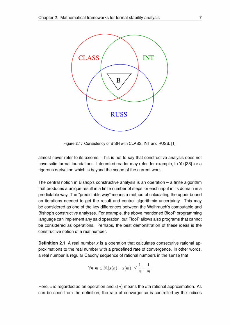
In 1967, E. Bishop published a monograph called "Foundations of Constructive Analy-sis" [37] where he revisited INT and developed a new kind of constructive mathematicsthat will be denoted by BISH here. BISH has the property that every proof in BISH is avalid proof in CLASS, INT and RUSS. Fig. 2.1 illustrates schematically this fact.
BISH can be described as mathematics with intuitionistic logical background along withcertain set-theoretical principles. Keeping the intuitionistic logical background and mak-ing sure that the set-theoretic principles would not imply non-constructive claims leadto a framework in which every proof could be interpreted as an algorithm. The goalof Bishop [37] was to develop an analysis that would, on one hand, implement theconstructive logic and be less formal so that anyone could use it without a strong back-ground in logic just like most of the engineers tacitly work in the classical set theory, but
Chapter 2: Mathematical frameworks for formal stability analysis 7
Figure 2.1: Consistency of BISH with CLASS, INT and RUSS. [1]
almost never refer to its axioms. This is not to say that constructive analysis does nothave solid formal foundations. Interested reader may refer, for example, to Ye [38] for arigorous derivation which is beyond the scope of the current work.
The central notion in Bishop’s constructive analysis is an operation – a finite algorithmthat produces a unique result in a finite number of steps for each input in its domain in apredictable way. The “predictable way” means a method of calculating the upper boundon iterations needed to get the result and control algorithmic uncertainty. This maybe considered as one of the key differences between the Weihrauch’s computable andBishop’s constructive analyses. For example, the above mentioned BlooP programminglanguage can implement any said operation, but FlooP allows also programs that cannotbe considered as operations. Perhaps, the best demonstration of these ideas is theconstructive notion of a real number.
Definition 2.1 A real number x is a operation that calculates consecutive rational ap-proximations to the real number with a predefined rate of convergence. In other words,a real number is regular Cauchy sequence of rational numbers in the sense that
∀n,m ∈ N.|x(n)− x(m)| ≤ 1n+
1m.
Here, x is regarded as an operation and x(n) means the nth rational approximation. Ascan be seen from the definition, the rate of convergence is controlled by the indices

8 Chapter 2: Mathematical frameworks for formal stability analysis
n and m themselves. Equality of two arbitrary real numbers is in general undecidablesince there is no algorithm that can decide whether x = y or x 6= y for x,y ∈ R. Such analgorithm would be equivalent to solving the problem of deciding whether an arbitrarycomputer program terminates or not – which is impossible as shown by Turing [32].Tosay, for example, that x < y means providing a witness or a certificate, a natural numbern∗ such that:
x(n∗)< y(n∗)− 1n∗
.
Further, a set is a pair of operations: ∈ determines that a given object is a member of theset, and = determines whenever two given set members are equal. Such a techniqueis common in constructive analysis – every statement comes together with a certificatethat verifies it. In turn, a proof means constructing a certificate. Treatment of logicalformulas is performed in this spirit.
For example, proving a formula ∃x∈ A.ϕ [x] means deriving an operation that constructsan instance x along with a proof that x ∈ A and a proof of the logical formula ϕ [x]. Thisoperation with the said proof is called a certificate of ∃x ∈ A.ϕ [x]. Proving a formula∀x ∈ A.ϕ [x] means proving a quantifier-free formula ϕ [x] with x being a free variableprovided with a certificate for x∈A. Working in constructive analysis is somewhat similarto programming which may be seen more appropriate for a certain group of controlsystem engineers than working in heavily abstract formal systems. On the other hand,any proof of a theorem in constructive analysis is (or can be made to) an algorithmwhose correctness proof is the proof of the theorem itself. As an important consequenceof constructive interpretation of analysis, the rule of excluded middle and in turn proofby contradiction is generally rejected.
The notion of a real number can generalized to the notion of a point in Euclidean spaceRn in a straightforward manner. Euclidean space Rn is a normed space with the norm
‖x‖,(
∑ni=1 (xi)
2) 1
2where xi is the ith coordinate of x.The metric is defined as ‖x− y‖
for any x,y ∈ Rn.
Particular attention is paid to those sets in Euclidean space which are called totallybounded:
Definition 2.2 A set X ⊂ Rn is called totally bounded if there is an operation that forany given positive rational number ε constructs a finite set {xi}N
i=1 of distinct points in Xsuch that any x ∈ X lies within an ε-ball centered at some xi.
An important property of totally bounded sets of the real number line is that their infimaand suprema exist constructively. Another important notion in constructive analysis isthe notion of a function:
Definition 2.3 A function f : Rn→ Rm is a pair of operations: one operation computes
Chapter 2: Mathematical frameworks for formal stability analysis 9
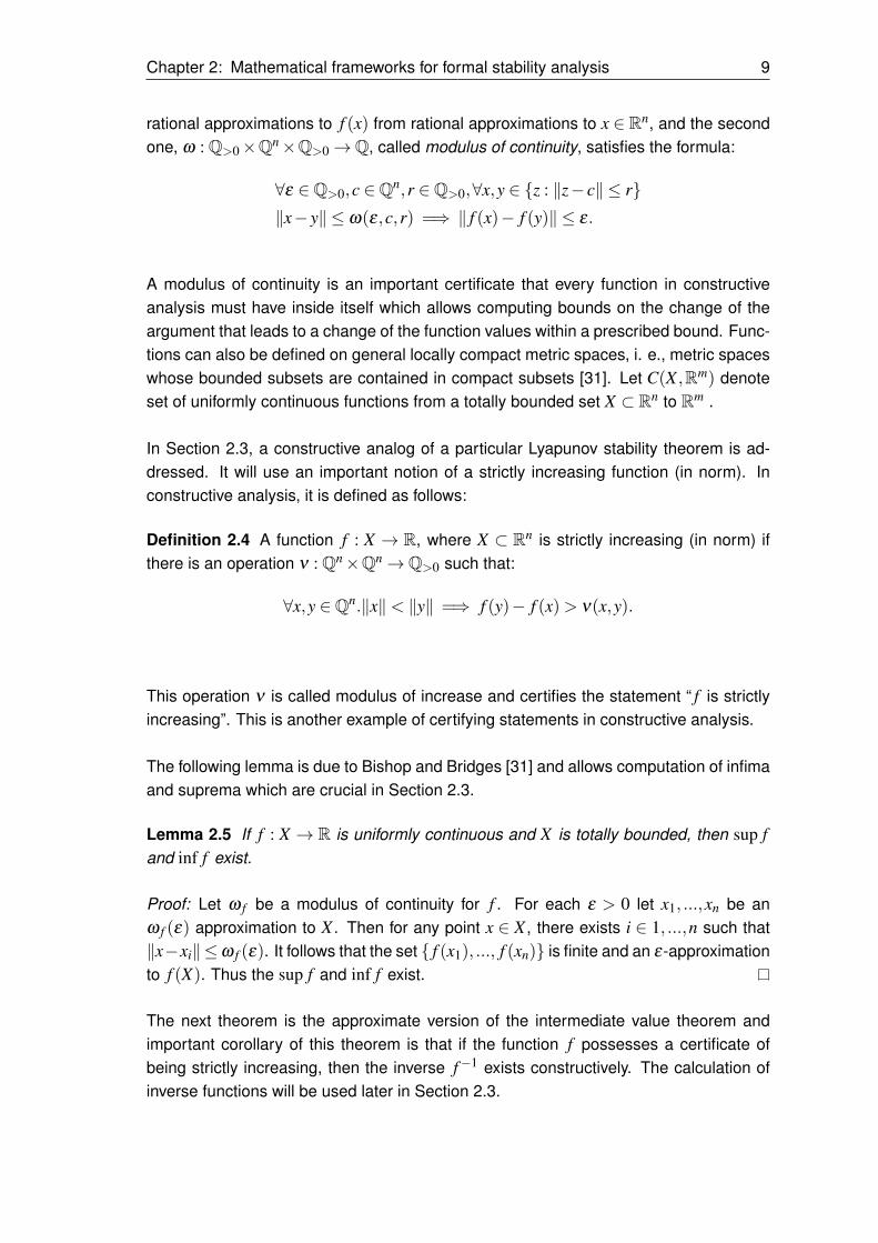
rational approximations to f (x) from rational approximations to x ∈ Rn, and the secondone, ω : Q>0×Qn×Q>0→Q, called modulus of continuity, satisfies the formula:
∀ε ∈Q>0,c ∈Qn,r ∈Q>0,∀x,y ∈ {z : ‖z− c‖ ≤ r}‖x− y‖ ≤ ω(ε,c,r) =⇒ ‖ f (x)− f (y)‖ ≤ ε.
A modulus of continuity is an important certificate that every function in constructiveanalysis must have inside itself which allows computing bounds on the change of theargument that leads to a change of the function values within a prescribed bound. Func-tions can also be defined on general locally compact metric spaces, i. e., metric spaceswhose bounded subsets are contained in compact subsets [31]. Let C(X ,Rm) denoteset of uniformly continuous functions from a totally bounded set X ⊂ Rn to Rm .
In Section 2.3, a constructive analog of a particular Lyapunov stability theorem is ad-dressed. It will use an important notion of a strictly increasing function (in norm). Inconstructive analysis, it is defined as follows:
Definition 2.4 A function f : X → R, where X ⊂ Rn is strictly increasing (in norm) ifthere is an operation ν : Qn×Qn→Q>0 such that:
∀x,y ∈Qn.‖x‖< ‖y‖ =⇒ f (y)− f (x)> ν(x,y).
This operation ν is called modulus of increase and certifies the statement “ f is strictlyincreasing”. This is another example of certifying statements in constructive analysis.
The following lemma is due to Bishop and Bridges [31] and allows computation of infimaand suprema which are crucial in Section 2.3.
Lemma 2.5 If f : X → R is uniformly continuous and X is totally bounded, then sup fand inf f exist.
Proof: Let ω f be a modulus of continuity for f . For each ε > 0 let x1, ...,xn be anω f (ε) approximation to X . Then for any point x ∈ X , there exists i ∈ 1, ...,n such that‖x−xi‖≤ω f (ε). It follows that the set { f (x1), ..., f (xn)} is finite and an ε-approximationto f (X). Thus the sup f and inf f exist.
The next theorem is the approximate version of the intermediate value theorem andimportant corollary of this theorem is that if the function f possesses a certificate ofbeing strictly increasing, then the inverse f−1 exists constructively. The calculation ofinverse functions will be used later in Section 2.3.

10 Chapter 2: Mathematical frameworks for formal stability analysis
Theorem 2.6 (Ye, [38]) If f ∈ C([a,b],R) and f (a) < f (b), then for any y such thatf (a) ≤ y ≤ f (b), and for any ε > 0, there exists x ∈ [a,b] such that | f (x)− y| < ε .Moreover if f is strictly increasing, then there exists x ∈ [a,b] such that f (x) = y.
Proof: Assume that ε > 0 is a rational number. Divide [a,b] into small intervals p0 =
a, ..., pN = b such that p1, ..., pN−1 are rational numbers and pi+1− pi≤ω f (ε/7), whereω f is a modulus of continuity for f . Therefore, | f (pi+1− f (pi))| ≤ ε/6. For each pi,we can choose a rational number qi such that | f (pi)−qi|< ε/6 and let q be a rationalsuch that |y− q| < ε/6. Then , |qi+1− qi| < ε/2. Since f (a) ≤ y ≤ f (b), we haveq0− ε/3 ≤ q ≤ qN + ε/3. By comparing q with q0, ...,qN , we can find qk such that|qk−q|< ε/2. Since | f (pk)−qk|< ε/6 and |y−q|< ε/6, we have | f (pk)−y|< ε .Forthe second half, note that f being strictly increasing implies that we have a term τ sothat for rational number p,q ∈ [a,b], if p < q, then t(p,q) is a positive rational numbersuch that f (q)− f (p) > t(p,q). That is, t(p,q) certificates that f (p) < f (q) for q > p.Then to estimate x such that f (x) = y up to the precision ε , we can divide [a,b] intosmall rational intervals each of length < ε/2 , and then for each interval [pi, pi+1] , wecan approach y up to the precision of t(pi, pi+1)/2 to decide if f (pi)< y or y < f (pi+1).The estimate of x will be pi+1 with pi the last one such that f (pi)< y.
Corollary 1 If f ∈C([a,b],R) and f is strictly increasing, then there exists the inversefunction g∈C([ f (a), f (b)],R), such that f (g(y)) = y for y∈ [ f (a), f (b)] and g( f (x)) = xfor x ∈ [a,b].
The next lemma allows extending functions on rational numbers to function of real num-bers. It will be used in Section 2.3.
Lemma 2.7 (Extension Lemma, Bishop and Bridges, [31]) Let Y be a dense subset ofa metric space X , and f : Y → Z a uniformly continuous function from Y to a completemetric space Z, with modulus of continuity ω f . Then there exists a uniformly continuousfunction g : X → Z with modulus of continuity 1
2ω f such that f (y) = g(y) for all y ∈ Y .
The next theorem is due to Ye [38] and adresses the initial value problems for the first-order ordinary differential equations which will also be used in Section 2.3 .
First, let a,b > 0, (t0,x0) ∈ R2,
D = [t0−a, t0 +a]× [x0−b,x0 +b]⊂ R2, (2.1)
Let f ∈C(D,R). The goal is to find a function χ(t) such that χ is differentiable on aninterval I = [t0− c, t0 + c],c≤ a, and (t,χ(t)) ∈ D for t ∈ I and
χ(t0) = x0, χ = f (t,χ(t)) (2.2)

Chapter 2: Mathematical frameworks for formal stability analysis 11
for x ∈ I. Such a function is called a solution of the initial value problem x(t0) = x0, x =f (t,x(t)). Function f (t,x) is called to satisfy the Lipschitz condition for x on D, if thereexists L such that
| f (t,x1)− f (t,x2)| ≤ L|x1− x2| (2.3)
Theorem 2.8 Suppose that f (t,x) is continuous on the rectangle D : |t− t0| ≤ a, |x−x0| ≤ b, and suppose that f (t,x) satisfies the Lipschitz condition for x on the rectangle.Let M = max{ f (t,x) : (x, t) ∈ D} and α = min(a,b/M). Then, there exists a uniquefunction χ differentiable on an interval I = [t0−α, t0 +α], such that χ(t0) = x0 andχ0(x) = χ(t,χ(t)) for t ∈ I. Moreover, χ depends on its initial value x0 uniformly contin-uously.
In the next section, a fragment of the Lyapunov stability theory relevant for the currentstudy is briefly described.

12 Chapter 2: Mathematical frameworks for formal stability analysis
2.2 Brief overview of Lyapunov stability theory
The following section describes briefly the Lyapunov stability theory relevant to the cur-rent study and is mainly based on Khalil, [39].
Consider the following dynamical system:
x = f (x, t),x ∈ Rn, t ∈ R≥0. (2.4)
Assume that xe = 0 is an equilibrium point of (2.4).
Definition 2.9 The equilibrium point x = 0 of (2.4) is ,
• stable if, for each ε > 0, there is δ = δ (ε, t0)> 0 such that
‖x(t0)‖< δ ⇒‖x(t)‖< ε,∀t ≥ t0 ≥ 0 (2.5)
• uniformly stable if, for each ε > 0, there is δ = δ (ε), independent of t0, such thatis satisfied.
• asymptotically stable if it is stable and there is c = c(t0)> 0 such that x(t)→ 0 ast→ ∞ for all ‖x(t0)‖ ≤ c.
• uniformly asymptotically stable if it is uniformly stable and there is c > 0, indepen-dent of t0, such that for all ‖x(t0)‖< c,x(t)→ 0 as t→ ∞.
In this study, attention is restricted to the concept of the uniform asymptotic stability.Stability properties of the equilibrium point may dependent in general on starting time t0(Khalil, [39]). For example, consider the following system:
x =− x1+ t
(2.6)
which has the closed-form solution
x(t) = x(t0)1+ t01+ t
(2.7)
The solutions are bounded via the condition ‖x(t)‖ ≤ ‖x(t0)‖. Here, the constant cdepends on t0. The concept of uniform stability with respect to the initial time makes cindependent from the starting time and is in the focus of the current work.
The following theorem states the necessary conditions for the equilibrium of (2.4) to beasymptotically stable [39, p. 100]:
Theorem 2.10 Let X ⊂ Rn contain the origin and V : X → R≥0 be a continuously dif-ferentiable function such that V (x) = 0⇔ x = 0 and V (x)< 0,x ∈ X \{0}. Then, xe = 0

Chapter 2: Mathematical frameworks for formal stability analysis 13
is asymptotically stable.
Proof: (Sketch) The theorem implies that xe = 0 is stable in the sense that for any ε
there exists a δ such that ‖x(0)‖ ≤ δ implies ‖x(t)‖ ≤ ε for all t ≥ 0. Fix an r ≤ ε . Itsuffices to show that for every χ , there exists τ such that ‖x(t)‖ ≤ χ for all t ≥ τ . SinceV (x(t)) is strictly decreasing and bounded below by zero, it follows that
limt→∞
V (x(t)) = v.
The fact that v = 0 can be shown by contradiction. Suppose that v > 0. Since V iscontinuous, there exists a d > 0 such that the closed ball Bd = {x : ‖x‖ ≤ d} ⊂ X iscontained in the set {x : V (x) ≤ v}. The condition v > 0 implies that the trajectory x(t)lies outside the ball Bd for all t ≥ 0. Define θ =de f −supd≤‖x‖≤r V (x). This assignmentis well-defined since the set {x : d ≤ ‖x‖ ≤ r} is compact and V is continuous. But
V (x(t)) =V (x(0))+t∫
0
V (x(τ))dτ ≤V (x(0))−θ · t.
The right-hand side must eventually become negative which contradicts the assumptionthat v > 0.
As was mentioned in Section 2, proof by contradiction is in general forbidden in con-structive analysis. The consequence for Theorem 2.10 is that although the limit of thenorm of the system trajectory is zero, there is no computable way to predict the rateof convergence. In fact, the very notion of a limit in classical analysis does not requirea computable rate of convergence. In the proof of the theorem, one might notice thatfor every χ , there exists a time τ after which the norm of the trajectory lies within χ ,but there is unfortunately no way to actually calculate this τ . This is a usual conse-quence of proof by contradiction: some object is claimed to exist, but no concrete wayof computing it is given. In contrast to this, every claim in constructive analysis comeswith a certificate. As for Definition 2.9, to say that limt→∞ ‖x(t)‖ = 0 means providinga certificate that allows computing a rate of convergence. Such a certificate may be apositive-definite strictly decreasing function defined in a way analogous to that in Defini-tion 2.4. This function then should serve as an upper bound on the norm of the systemtrajectory.
In the next section, the Lyapunov asymptotic stability theorem is revisited construc-tively.

14 Chapter 2: Mathematical frameworks for formal stability analysis
2.3 Constructive stability analysis
In this section, the Lyapunov asymptotic stability theorem is addressed from the stand-point of constructive analysis as per Section 2. The goal is to obtain a constructivecounterpart that would allow computation of the convergence certificates described inthe previous section. First some basics of theorem proving tactics in constructive anal-ysis are described. Then, Proposition 2.3.1 is stated and proven constructively followedby a particular algorithmic realization.
Two basics tactics in developing constructive counterparts of classical theorems arepossible in constructive analysis. Sometimes, but rarely, the theorem can be provenconstructively as it stands. But if not, there are two ways: one is to relax the claim ofthe theorem, e. g., prove an approximate version of the theorem, whereas the second isto strengthen the assumptions. In this section, the second way is chosen. As was dis-cussed in Section 2, the classical Lyapunov stability theorem does not allow computinga convergence certificate. The goal of this section is to investigate the computationalcontent of the stability theorem and to extract a particular algorithmic realization thatcalculates the rate of convergence of the system trajectories in norm. The followingproposition is based on Theorem 3.8 of [39] and is the core of the current study:
Proposition 2.3.1 ( See [40]) Let X be the closed unit ball in Rn centered at the originand x = f (x, t),x ∈ X be a dynamical system with the equilibrium point xe = 0, such thatf (x, t) is Lipschitz-continuous in x. Suppose that there exists a continuously differen-tiable function V : X× [0,∞)→ R with the following properties:
1. There exists a strictly increasing function w1 : X → R such that
∀t ≥ 0.∀x ∈ X .w1(x)≤V (x, t)
w1(0) = 0.
2. There exists a function w2 : X → R,w2(0) = 0, a positive rational number ξ suchthat
∀‖x‖ ≥ ‖y‖.w2(x)−w2(y)≥ ξ (‖x‖−‖y‖),
and ∀t ≥ 0.∀x ∈ X .V (x, t)≤ w2(x).
3. There exists a Lipschitz-continuous strictly increasing function w3 : X→R,w3(0)=0 such that
∀t ≥ 0.∀x ∈ X .V (x, t)≤−w3(x)
Then, xe = 0 is asymptotically stable for any x(0) ∈ X .

Chapter 2: Mathematical frameworks for formal stability analysis 15
Proof: Define the following functions:
α1(s) =de f infs≤‖x‖≤1
w1(x)
α2(s) =de f sup‖x‖≤s
w2(x)
α3(s) =de f infs≤‖x‖≤1
w3(x)
for any rational s ∈ [0,1]. First, observe that a sphere Sr =de f {x : ‖x‖= r},r ∈Q is atotally bounded set since a sequence of points with pure rational coordinates on S canbe constructed that ε-approximates any point on S for any given ε . Consequently, theset A =de f {x : s≤‖x‖≤ r}⊂Rn,s,r ∈Q is also totally bounded. The certificate of totalboundedness can be constructed by appropriately choosing radii of concentric spheresand approximating each one including Ss and Sr. Since the functions w1,w2 and w3 arecontinuous, the functions α1, α2, α3 are constructively well-defined by Lemma 2.5. ByLemma 2.7 , α1, α2, α3 can be extended to the entire unit interval. Denote the extensionsby α1,α2,α3 respectively. By Theorem 2.6, it follows that the inverse function α
−12 can
be constructed since α2 is a continuous strictly monotonic function on a compact set.Moreover, α
−12 is strictly increasing and Lipschitz-continuous, since α2 by construction
satisfies the following condition:
∀s≥ r.α2(s)−α2(r)≥ ξ (s− r)
To see this, observe that s = α−12 (s′) and r = α
−12 (r′) for some s′,r′ in the respective
domains. Then, the condition implies that
α2(α−12 (s′))−α2(α
−12 (r′))≥ ξ (α−1
2 (s′)−α−12 (r′))
which yields
(α−12 (s′)−α
−12 (r′))≤ 1
ξ(s′− r′).
The following conditions evidently hold:
α1(‖x‖)≤V (x, t)≤ α2(‖x‖),V (x, t)≤ α3(‖x‖)
for any t ≥ 0 and x ∈ X . Further,by Theorem 2.8, since f is Lipschitz-continuous andX is compact, system trajectories starting from all x0 ∈ X exist. The next step is toshow boundedness of the system trajectories. To this end, notice that since w1 is strictlyincreasing, it follows that α1 is a strictly increasing continuous function on a compactset and α
−11 in turn exists and is also strictly increasing. It follows that α
−11 (V0)≥ ‖x0‖.
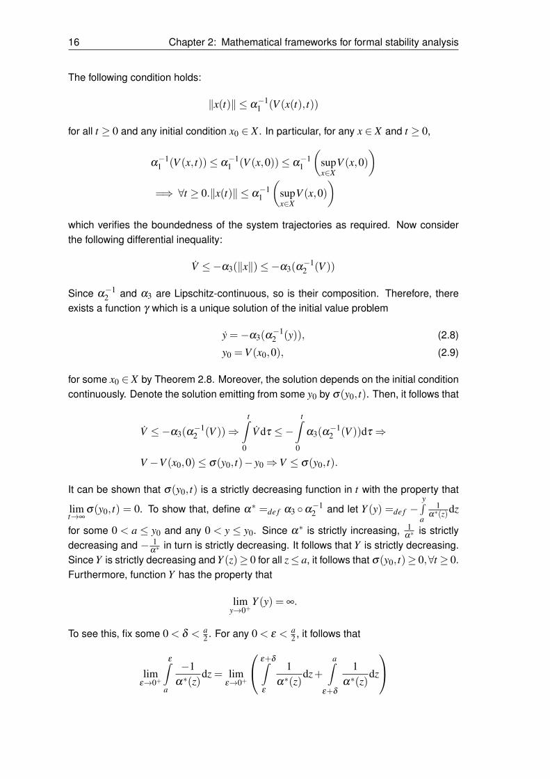
16 Chapter 2: Mathematical frameworks for formal stability analysis
The following condition holds:
‖x(t)‖ ≤ α−11 (V (x(t), t))
for all t ≥ 0 and any initial condition x0 ∈ X . In particular, for any x ∈ X and t ≥ 0,
α−11 (V (x, t))≤ α
−11 (V (x,0))≤ α
−11
(supx∈X
V (x,0))
=⇒ ∀t ≥ 0.‖x(t)‖ ≤ α−11
(supx∈X
V (x,0))
which verifies the boundedness of the system trajectories as required. Now considerthe following differential inequality:
V ≤−α3(‖x‖)≤−α3(α−12 (V ))
Since α−12 and α3 are Lipschitz-continuous, so is their composition. Therefore, there
exists a function γ which is a unique solution of the initial value problem
y =−α3(α−12 (y)), (2.8)
y0 =V (x0,0), (2.9)
for some x0 ∈ X by Theorem 2.8. Moreover, the solution depends on the initial conditioncontinuously. Denote the solution emitting from some y0 by σ(y0, t). Then, it follows that
V ≤−α3(α−12 (V ))⇒
t∫0
V dτ ≤−t∫
0
α3(α−12 (V ))dτ ⇒
V −V (x0,0)≤ σ(y0, t)− y0⇒V ≤ σ(y0, t).
It can be shown that σ(y0, t) is a strictly decreasing function in t with the property that
limt→∞
σ(y0, t) = 0. To show that, define α∗ =de f α3 ◦α−12 and let Y (y) =de f −
y∫a
1α∗(z)dz
for some 0 < a ≤ y0 and any 0 < y ≤ y0. Since α∗ is strictly increasing, 1α∗ is strictly
decreasing and − 1α∗ in turn is strictly decreasing. It follows that Y is strictly decreasing.
Since Y is strictly decreasing and Y (z)≥ 0 for all z≤ a, it follows that σ(y0, t)≥ 0,∀t ≥ 0.Furthermore, function Y has the property that
limy→0+
Y (y) = ∞.
To see this, fix some 0 < δ < a2 . For any 0 < ε < a
2 , it follows that
limε→0+
ε∫a
−1α∗(z)
dz = limε→0+
ε+δ∫ε
1α∗(z)
dz+a∫
ε+δ
1α∗(z)
dz

Chapter 2: Mathematical frameworks for formal stability analysis 17
≥ limε→0+
δ
α∗(ε +δ )+
a∫ε+δ
1α∗(z)
= ∞
since α∗(0) = 0. On any compact set [ε,y0],ε > 0, Y−1 exists and for any t ≤ t∗ =de f
Y (ε)+Y (y0) it follows that
σ(y0, t) = Y−1(Y (y0)+ t)≤ ε
due to the fact thatY (σ(y0, t))−Y (y0) = t
and because Y is strictly decreasing. For any ε1 > ε , it follows that for all t∗≤ t ≤ t∗1 =de f
Y (ε1)+Y (y0),σ(y0, t)< σ(y0, t∗)≤ ε.
Therefore, for any ε > 0 there exists a t∗ such that σ(y0, t)≤ ε for all t ≥ t∗ which means
limt→∞
σ(y0, t) = 0.
Since ‖x(t)‖ ≤ α−11 (σ(y0, t)) =de f γ(y0, t) for all t ≥ 0 and any initial condition x0 ∈ X ,
it follows that limt→∞‖x(t)‖= 0 for any x0 in X .
Proposition 2.3.1 can be seen as a possible constructive counterpart of Theorem 2.10of Section 2.2. According to the requirement that an asymptotically stable equilibriumneeds to possess a convergence certificate, the strictly decreasing function γ(y0, t) canbe seen as a convergence certificate. It can be used to assess how fast the systemtrajectories decay to zero in norm. Setting supx∈X V (x,0) as the initial condition in theproblem (2.9), a particular certificate γ(t) can be computed which indicates the “worst”bound on the norm of the system trajectories for the given functions w1,w2,w3. Such a“worst” convergence certificate will be in the focus of the case study in Section 2.5.

18 Chapter 2: Mathematical frameworks for formal stability analysis
2.4 Algorithmic realization
Further, Proposition 2.3.1 can be realized in the following simple algorithms. The firstone, Algorithm 1, certifies the fact that the annuli {x : s ≤ ‖x‖r},s,r ∈ Q used in theproof are totally bounded.
Algorithm 1 Construction of a total boundedness certificate for {x : s ≤ ‖x‖ ≤ r} ⊂R2,s,r ∈QRequire: ε ∈Q and s,r ∈Q,0≤ s≤ r ≤ 1
Initialize S =de f /0if r = 0 then
Add point (0,0) to Sfor a ∈ {s,s+ ε, . . . ,r} do
θa =de f 2arcsin( ε
2a)for θ ∈ {0,θa,2θa, . . . ,2π} do
Add point (acos(θ),asin(θ)) to Sreturn S
For demonstration purposes, the two-dimensional case is considered. For the casex ∈ Rn,n > 2, this algorithm would require a modification, but it is beyond the scope ofthe current study. In Algorithm 1, sin,cos,arcsin need to be approximated sufficiently.The second one, Algorithm 2, computes the function infr≤‖x‖≤1 f for a scalar-valuedfunction f on the unit ball of R2.
Algorithm 2 Construction of infr≤‖x‖≤1 fRequire: ε ∈Q,r ∈Q,0≤ r ≤ 1 and a function f
Set δ such that ∀x,y.‖x− y‖ ≤ δ =⇒ | f (x)− f (y)| ≤ ε
Call Algorithm 1 with the parameters (δ ,r,1) and get a total boundedness certificateSreturn minS f (S)
An algorithm for computing sup0≤‖x‖≤r f ,r ≤ 1 is analogous to Algorithm 2.

Chapter 2: Mathematical frameworks for formal stability analysis 19
The next algorithm, Algorithm 3, computes the inverse of a strictly increasing function.
Algorithm 3 Construction of f−1 for a function f : I→R where I is a non-trivial intervalRequire: ε,y ∈ range( f ) and a function f
Set P to be a partition of I into subintervals of length less than ε
2Decide for each subinterval [pi, pi+1] ∈ P whether f (pi)< y or y < f (pi+1)return pi+1 such that f (pi)< y
In Algorithm 3, the second step is constructively valid since there is a modulus of in-crease within f that allows the case distinction f (pi) < y or y < f (pi+1). Solutions ofinitial value problems can be computed by Picard iteration provided that the subject func-tion satisfies the Lipschitz condition in the domain of interest [41]. Constructive proof ofthe Picard-Lindelöf theorem and details of the algorithm may be found in [38]. The cur-rent section was concerned with development of a constructive counterpart of Theorem2.10 on asymptotic stability which resulted in Proposition 2.3.1. A particular algorith-mic realization was provided. The next section demonstrates a particular application ofthese algorithms to investigating stability of a sample dynamical system.

20 Chapter 2: Mathematical frameworks for formal stability analysis
2.5 Case study and discussion
Application of Proposition 2.3.1 is demonstrated for the following nonlinear dynamicalsystem:
x1 =− x1 + x1e−x2
1
1+ x21− x2 tanh(t),
x2 =− x2 + x2e−t2
1+ x22+ x1 tanh(t).
(2.10)
It can be shown that V (x, t)≡ v‖x‖2 is a Lyapunov function for the system (2.10) for anypositive number v. By setting
w1(x) :=v‖x‖2,
w2(x) :=
{vχ‖x‖,‖x‖ ≤ χ,
vχ‖x‖2,‖x‖ ≥ χ
w3(x) :=2v
(‖x‖2− x2
1e−x2
1
1+ x21−
x22
1+ x22
),
for any rational number 0 < χ < 1 the conditions of Proposition 2.3.1 are satisfied andthe convergence certificate can be thus computed. In the current study, χ was set to0.1. Fig. 2.2 illustrates the function w3 for the case v = 1
2 which is commonly used instability analyses.
0
1 1
1
Figure 2.2: Function w3 – upper bound on the derivative of the Lyapunov function

Chapter 2: Mathematical frameworks for formal stability analysis 21
5 10 15
0.5
0
1
Figure 2.3: Convergence certificate and example system trajectories
The certificate γ as per Proposition 2.3.1 was computed. As can bee seen in Fig.2.3, which illustrates the norm of several example system trajectories, the certificate forv = 1
2 is relatively conservative. For testing purposes, another certificate – for v = 120 –
is illustrated as well.
Fig. 2.4 illustrates how the certificate for v = 120 bounds some example system trajecto-
ries.
1
1
15
Figure 2.4: Three-dimensional illustration of the convergence certificate and example systemtrajectories
22 Chapter 2: Mathematical frameworks for formal stability analysis
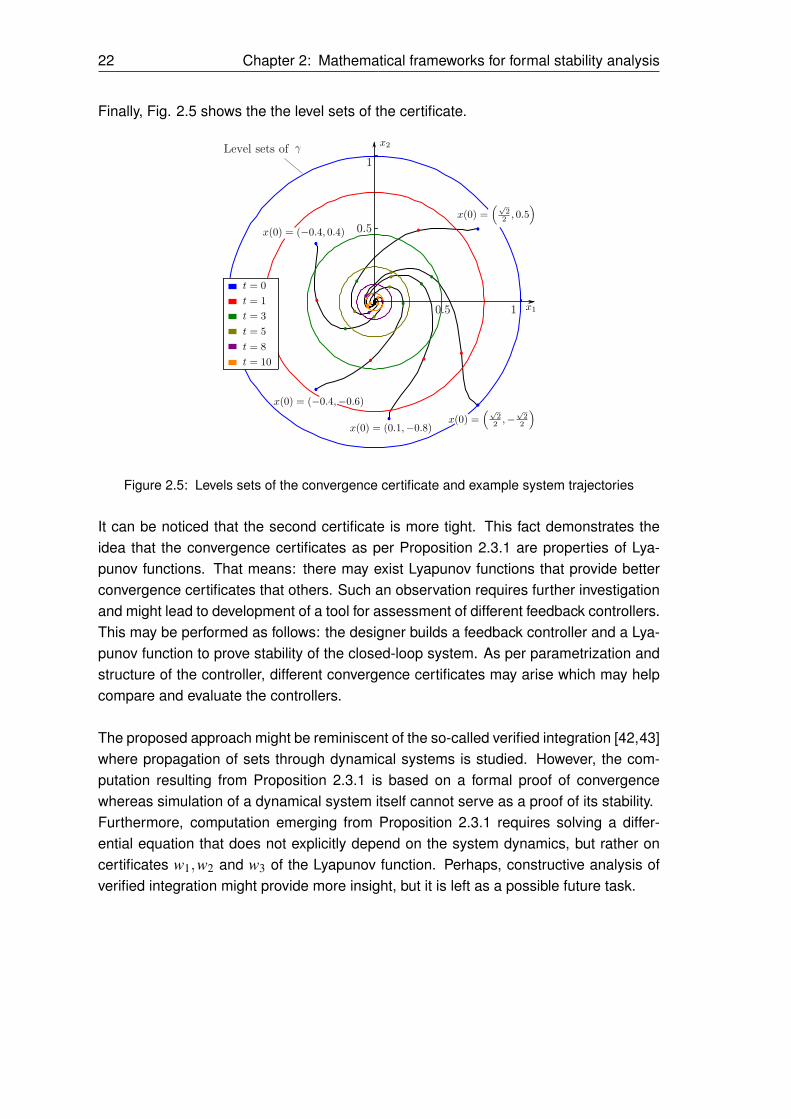
Finally, Fig. 2.5 shows the the level sets of the certificate.
0.5
1
0.5 1
Level sets of
Figure 2.5: Levels sets of the convergence certificate and example system trajectories
It can be noticed that the second certificate is more tight. This fact demonstrates theidea that the convergence certificates as per Proposition 2.3.1 are properties of Lya-punov functions. That means: there may exist Lyapunov functions that provide betterconvergence certificates that others. Such an observation requires further investigationand might lead to development of a tool for assessment of different feedback controllers.This may be performed as follows: the designer builds a feedback controller and a Lya-punov function to prove stability of the closed-loop system. As per parametrization andstructure of the controller, different convergence certificates may arise which may helpcompare and evaluate the controllers.
The proposed approach might be reminiscent of the so-called verified integration [42,43]where propagation of sets through dynamical systems is studied. However, the com-putation resulting from Proposition 2.3.1 is based on a formal proof of convergencewhereas simulation of a dynamical system itself cannot serve as a proof of its stability.Furthermore, computation emerging from Proposition 2.3.1 requires solving a differ-ential equation that does not explicitly depend on the system dynamics, but rather oncertificates w1,w2 and w3 of the Lyapunov function. Perhaps, constructive analysis ofverified integration might provide more insight, but it is left as a possible future task.

Chapter 3: Conclusion 23
3 Conclusion
This work suggested to formally study a fragment of the Lyapunov stability theory withthe goal of addressing algorithmic uncertainty. As the foundation, constructive analysiswas proposed. Unlike several existing formal approaches, constructive analysis is lessloaded with abstract logical derivations and is closer to the usual classical analysis thata control systems engineer is familiar with. It is believed that such an approach mayhave its merit for control theory. It was indicated which parts of the classical asymptoticstability theorem did not provide computable results, and in contrast to it, a constructivecounterpart was proven which was based on so called certificates. Algorithm extractionwas demonstrated for calculating the convergence certificates. A case study showedresults of computation convergence certificates for an example dynamical system.

24

25
Bibliography
[1] D. S. Bridges and I. Loeb. Glueing continuous functions constructively. Archive forMathematical Logic, 49(5):603–616, 2010.
[2] O. Russell. Certified exact transcendental real number computation in coq. InInternational Conference on Theorem Proving in Higher Order Logics, pages 246–261. Springer, 2008.
[3] S. Boldo, C. Lelay, and G. Melquiond. Formalization of real analysis: A surveyof proof assistants and libraries. Mathematical Structures in Computer Science,pages 1–38.
[4] L. Cruz-Filipe, H. Geuvers, and F. Wiedijk. C-corn, the constructive coq repositoryat nijmegen. In International Conference on Mathematical Knowledge Manage-ment, pages 88–103. Springer, 2004.
[5] B. Akbarpour and L. C. Paulson. Metitarski: An automatic theorem prover for real-valued special functions. Journal of Automated Reasoning, 44(3):175–205, 2010.
[6] N. Julien. Certified Exact Real Arithmetic Using Co-induction in Arbitrary IntegerBase, pages 48–63. Springer Berlin Heidelberg, Berlin, Heidelberg, 2008.
[7] T. C. Hales, J. Harrison, S. McLaughlin, T. Nipkow, S. Obua, and R. Zumkeller.A revision of the proof of the kepler conjecture. In The Kepler Conjecture, pages341–376. Springer, 2011.
[8] A. M. Lyapunov. The General Problem of the Stability of Motion (in Russian). In-ternational Journal of Control, 55(3):531–534, 1992.
[9] A. Platzer. Logics of dynamical systems. In Proceedings of the 2012 27th An-nual IEEE/ACM Symposium on Logic in Computer Science, LICS’12, pages 13–24.IEEE Computer Society, 2012.
[10] D. Araiza-Illan, K. Eder, and A. Richards. Formal verification of control systems’properties with theorem proving. In Control (CONTROL), 2014 UKACC Interna-tional Conference on, pages 244–249, 2014.
[11] M. Althoff and J. M. Dolan. Online verification of automated road vehicles usingreachability analysis. IEEE Transactions on Robotics, 30(4):903–918, 2014.

26
[12] M. Althoff. Formal and compositional analysis of power systems using reachablesets. IEEE Transactions on Power Systems, 29(5), 2014.
[13] S. Gao. Descriptive control theory: A proposal. arXiv preprint arXiv:1409.3560,2014.
[14] H. Kong, F. He, X. Song, M. Gu, H. Tan, and J. Sun. Safety verification of semi-algebraic dynamical systems via inductive invariant. Tsinghua Science and Tech-nology, 19(2):211–222, 2014.
[15] U. Siddique, O. Hasan, and S. Tahar. Formal modeling and verification of integratedphotonic systems. In In Proceedings of the 9th Annual IEEE International SystemsConference (SysCon), pages 562–569, 2015.
[16] M. Chan, D. Ricketts, S. Lerner, and G. Malecha. Formal verification of stabilityproperties of cyber-physical systems. 2016.
[17] C. Livadas. Formal verification of safety-critical hybrid systems. MassachusettsInstitute of Technology, 1997.
[18] M. Fränzle. Analysis of hybrid systems: An ounce of realism can save an infinityof states. In International Workshop on Computer Science Logic, pages 126–139.Springer, 1999.
[19] V. Mysore, C. Piazza, and B. Mishra. Algorithmic algebraic model checking ii: De-cidability of semi-algebraic model checking and its applications to systems biology.In International Symposium on Automated Technology for Verification and Analysis,pages 217–233. Springer, 2005.
[20] A. Platzer and J.-D. Quesel. European train control system: A case study in formalverification. In International Conference on Formal Engineering Methods, pages246–265. Springer, 2009.
[21] A. Tarski. A decision method for elementary algebra and geometry. In Quanti-fier Elimination and Cylindrical Algebraic Decomposition, pages 24–84. Springer,1998.
[22] S. M. Loos, D. Renshaw, and A. Platzer. Formal verification of distributed aircraftcontrollers. In Proceedings of the 16th international conference on Hybrid systems:computation and control, pages 125–130. ACM, 2013.
[23] L. Zou, J. Lv, S. Wang, N. Zhan, T. Tang, L. Yuan, and Y. Liu. Verifying chinesetrain control system under a combined scenario by theorem proving. In Working

27
Conference on Verified Software: Theories, Tools, and Experiments, pages 262–280. Springer, 2013.
[24] A. Platzer. Differential dynamic logics-automated theorem proving for hybrid sys-tems. PhD thesis, Universität Oldenburg, 2008.
[25] A. Platzer and J.-D. Quesel. Keymaera: A hybrid theorem prover for hybrid systems(system description). In International Joint Conference on Automated Reasoning,pages 171–178. Springer, 2008.
[26] D. Araiza-Illan, K. Eder, and A. Richards. Verification of control systems imple-mented in simulink with assertion checks and theorem proving: A case study. In InProceedings of the 2015 European Control Conference (ECC), pages 2670–2675.IEEE, 2015.
[27] K. Weihrauch. Computability, EATCS Monographs in Theoretical Computer Sci-ence. Springer Verlag, 1987.
[28] K. Weihrauch. A foundation for computable analysis. In International Conferenceon Current Trends in Theory and Practice of Computer Science, pages 104–121.Springer, 1997.
[29] K. Weihrauch. Computable Analysis: an Introduction. Springer Science & BusinessMedia, 2012.
[30] C. Bernardeschi and A. Domenici. Verifying safety properties of a nonlinear controlby interactive theorem proving with the prototype verification system. InformationProcessing Letters, 116(6):409–415, 2016.
[31] E. Bishop and D. Bridges. Constructive analysis, volume 279. Springer Science &Business Media, 1985.
[32] A. Turing. On computable numbers, with an application to the entscheidungsprob-lem. J. of Math, 58(345-363):5, 1936.
[33] D. Hofstadter. Gödel, Escher, Bach, 1975.
[34] L.E.J. Brouwer. On the Foundations of Mathematics. Ph.D. thesis, 1907.
[35] R.S. Buss. Handbook of proof theory. volume 137. Elsevier, 1998.
[36] A. S. Troelstra. History of constructivism in the 20th century.

28 Chapter 3: Conclusion
[37] E. Bishop. Foundations of constructive analysis, volume 60. McGraw-Hill NewYork, 1967.
[38] F. Ye. Strict finitism and the logic of mathematical applications. Springer, 2011.
[39] H. Khalil. Nonlinear Systems. Prentice-Hall, 1996.
[40] P. Osinenko, G. Devadze, and S. Steif. Constructive analysis of control sys-tems stability (submitted manuscript). In In Proceedings of the 20th IFAC WorldCongress, 2016.
[41] E. Coddington and N. Levinson. Theory of Ordinary Differential Equations. NewYork: McGraw-Hill, 1955.
[42] M. Berz and K. Makino. Verified integration of odes and flows using differentialalgebraic methods on high-order taylor models. Reliable Computing, 4(4):361–369, 1998.
[43] M. Berz, K. Makino, and J. Hoefkens. Verified integration of dynamics in the so-lar system. Nonlinear Analysis: Theory, Methods & Applications, 47(1):179–190,2001.
Erklärung 29
Erklärung
Hiermit erkläre ich, dass ich meine Arbeit selbstständig verfasst, keine anderen als dieangegebenen Quellen und Hilfsmittel benutzt und die Arbeit noch nicht anderweitig fürPrüfungszwecke vorgelegt habe.
Stellen, die wörtlich oder sinngemäß aus Quellen entnommen wurden, sind als solchekenntlich gemacht.
Mittweida, 14. Dezember 2016
HSMW-Thesis v 2.0