University of Liège

Faculty of Applied Sciences

Master Thesis

Optimisation of a demand-responsive transit system

Author : Corentin Pirson

Supervisors : Mario Cools and Quentin Louveaux

Master thesis submitted for the degree of

MSc in Physical Engineering

Academic year 2016-2017

ii

Remerciements

Je tiens tout d’abord à remercier sincèrement mes promoteurs Messieurs Quentin Louveaux etMario Cools qui m’ont guidé et encouragé dans l’accomplissement de ce travail tout au long del’année. Je remercie également Thibaut Cuvelier de m’avoir fait découvrir l’optimisation dis-crète. Ses conseils dans les premiers pas de ce projet ont été précieux.

Merci à Madame Sabine Limbourg et Monsieur Bertrand Cornélusse d’avoir accepté de fairepartie du jury de ce travail de fin d’études. Je leur souhaite une agréable lecture.

Je désire tout particulièrement remercier Kevin Bulthuis pour la relecture et les conseils avisésqu’il m’a donnés pour parachever ce mémoire. Son aide dans ce cadre ne représente qu’une in-fime partie de ce qu’il a pu m’ apporter durant 10 années de discussions multidisciplinaires dansles transports en commun.

Mes remerciements vont enfin à ma famille qui a largement contribué à ce que mes étudeset ce mémoire puissent être menés à bien dans des conditions optimales.

iii

Optimisation of a demand-responsive transit systemPirson Corentin – Master in physical engineering – 2016-2017

The development of technologies such as GPS, real time operating smartphone applications andautonomous vehicles in a relatively near future allow to think about ways of reinventing publictransport. A way to make it more flexible is to replace classical bus lines by a fleet of publicvehicles that would systematically adapt their route to serve clients. This work aims at studyingsuch a system from an optimisation point of view. The objective is, given origin and destinationpoints of the clients, to optimise the routes of the di�erent vehicles of the fleet. The optimisationis based on the satisfaction of the clients, i.e. on the minimisation of the time spent waitingfor a vehicle and inside this vehicle. The equity of the service among the di�erent clients isalso taken into account. It is established in this work that the problem can be modelled asa Vehicle Routing Problem for which the objective function is adapted. An algorithm basedon the simulated annealing metaheuristic method is developed in order to optimise the routesof the vehicles under di�erent hypotheses. The model is applied in several situations (generaltrips demand in a large area and peak hour situation in an idealised city) in order to assess theperformances of the system. The system appears to be more e�cient in high demand-densityareas such as the centres of big cities. For more general travel demand, the combination of sucha system with more classical mass transport systems should be considered.

Key-words: transport planning, discrete optimisation, Vehicle Routing Problem, simulatedannealing.

iv

Contents

Table of Contents . . . . . . . . . . . . . . . . . . . . . . . . . . . . . . . . . . . . . . . 1

1 Introduction 3

1.1 Related work . . . . . . . . . . . . . . . . . . . . . . . . . . . . . . . . . . . . . . 41.2 Problems to be solved . . . . . . . . . . . . . . . . . . . . . . . . . . . . . . . . . 6

1.2.1 Demand: where and when clients want to go . . . . . . . . . . . . . . . . 71.2.2 Geography: definition of time costs and saturation of roads . . . . . . . . 81.2.3 Objective: definition of the optimisation criteria . . . . . . . . . . . . . . 81.2.4 Fleet: characteristics of the available vehicles . . . . . . . . . . . . . . . . 91.2.5 Limiting the number of taxi stop points . . . . . . . . . . . . . . . . . . . 91.2.6 Structure in the network . . . . . . . . . . . . . . . . . . . . . . . . . . . . 9

2 Mathematical formulation of the optimisation problems 11

2.1 Vehicles with one passenger capacity (car sharing) . . . . . . . . . . . . . . . . . 112.1.1 Problem seen as a task scheduling problem with several machines . . . . . 122.1.2 Inspiration from the Vehicle Programming Problem . . . . . . . . . . . . 14

2.2 Problem seen as a variation of the classical VRP (the MinAvg and the MinMaxproblems) . . . . . . . . . . . . . . . . . . . . . . . . . . . . . . . . . . . . . . . . 17

2.3 Vehicles with capacity of more than one passenger (ride sharing) . . . . . . . . . 202.4 Adding release times . . . . . . . . . . . . . . . . . . . . . . . . . . . . . . . . . . 202.5 Towards more fairness . . . . . . . . . . . . . . . . . . . . . . . . . . . . . . . . . 21

3 Methodology of resolution 23

3.1 Local search and metaheuristics . . . . . . . . . . . . . . . . . . . . . . . . . . . . 233.1.1 Solution space and local search. . . . . . . . . . . . . . . . . . . . . . . . . 233.1.2 Metaheuristics . . . . . . . . . . . . . . . . . . . . . . . . . . . . . . . . . 25

3.2 Simulated annealing . . . . . . . . . . . . . . . . . . . . . . . . . . . . . . . . . . 253.2.1 Principle . . . . . . . . . . . . . . . . . . . . . . . . . . . . . . . . . . . . 253.2.2 The cooling schedule . . . . . . . . . . . . . . . . . . . . . . . . . . . . . . 253.2.3 Summary . . . . . . . . . . . . . . . . . . . . . . . . . . . . . . . . . . . . 26

3.3 Application to the combined MinSum and MinMax VRP . . . . . . . . . . . . . 263.3.1 Car sharing problem: local search for a combined MinSum-Minmax VRP

variation . . . . . . . . . . . . . . . . . . . . . . . . . . . . . . . . . . . . . 263.3.2 Ride sharing problem with maximum arrival times . . . . . . . . . . . . . 313.3.3 Ride sharing with maximum relative arrival time . . . . . . . . . . . . . . 333.3.4 Multi-passengers vehicles with release times . . . . . . . . . . . . . . . . . 34

3.4 Performances of the method . . . . . . . . . . . . . . . . . . . . . . . . . . . . . . 343.4.1 Computation times . . . . . . . . . . . . . . . . . . . . . . . . . . . . . . . 343.4.2 Quality of the solutions . . . . . . . . . . . . . . . . . . . . . . . . . . . . 37

3.5 Avenues of improvement . . . . . . . . . . . . . . . . . . . . . . . . . . . . . . . . 383.5.1 Ameliorations for the simulated annealing process . . . . . . . . . . . . . 403.5.2 Pre-processing of the data (clustering) . . . . . . . . . . . . . . . . . . . . 41

1

4 Results analysis 44

4.1 Solved problems definitions and notations . . . . . . . . . . . . . . . . . . . . . . 444.2 Influence of the weight factors W . . . . . . . . . . . . . . . . . . . . . . . . . . . 46

4.2.1 Evolution of the maximum waiting time with W (Problem 1) . . . . . . . 464.2.2 Penalty factor of Problem 4 . . . . . . . . . . . . . . . . . . . . . . . . . . 474.2.3 Quality of service as a function of the distance from the center . . . . . . 48

4.3 Influence of the demand density on the quality of the service. Modelling withproblems 2 and 4. . . . . . . . . . . . . . . . . . . . . . . . . . . . . . . . . . . . . 504.3.1 Influence of the density of the demand . . . . . . . . . . . . . . . . . . . . 504.3.2 Other considerations . . . . . . . . . . . . . . . . . . . . . . . . . . . . . . 50

4.4 Quality of the service as a function of the available fleet . . . . . . . . . . . . . . 52

5 Conclusions and perspectives 55

2

Chapter 1

Introduction

Nowadays, in order to contribute to the reduction of the number of vehicles on the roads andthe subsequent problems of congestion inside the cities and on the main axes, citizen havemainly two alternatives to the use of their individual car to achieve their daily displacements :classical public transports (bus, train, tramway and underground) and car sharing. Except invery specific cases (living and working next to train stations linked by direct lines, displacementsinside a city along well deserved axes, same place and hours of work as a neighbour), the practiceof these alternatives requires the user to be flexible and to adapt departure and arrival timesconsequently. The time devoted to commuting can be significantly increased.

These flexibility requirements reflect a mismatch between the transport o�er and demand,especially for specific journeys that are performed by a limited number of people. The simpleexample of the bus service of countryside areas (except school services) is self speaking : only afew buses serve the area each day, and only a very low number of people can be flexible enoughto use them. This situation leads to economic and ecological aberrations.

There is thus a huge interest in working at a more refined adaptation of such transportationsystems to the demand in order to make them more e�cient on the user point of view, but alsomore sustainable on economic and ecological aspects. The development of the GPS technologyin the past decades as well as systematisation of fast and easy communication between usersand transport networks more recently (real time operating smartphone applications,...) allowto think about ways of reinventing public transport. The upcoming technology of autonomouscars reinforces the idea of the possibility of an optimised and demand-based transport network.

This thesis focuses on a system that unifies the features of public transport, as it will becomposed of a fleet of public vehicles (e.g. taxis or autonomous cars) and of car sharing, asthese vehicles are expected to take along their routes several users from their own startingpoints and to their destinations. The satisfaction of the users will be used as a depart criterionfor determining possible operation of the system, and the economical and environmental impactof such a system will be deduced and studied in a second time. It is clear that if the circulationconditions are kept as they are, the use of such a system cannot be advantageous in terms oftravel times. However, one of the objective of such a system, as a public transport system, isto lower the number of vehicles on the roads. This is expected to decrease travel times due tocongestion.

In this work, the fact that the mentioned vehicles are autonomous or not is not crucial :the focus is set on the planning of the routes they follow. However, in subsequent works, thedi�erence between classical taxis and autonomous vehicles could be taken into account, theautonomous cars allowing to predict travel times more precisely (if the circulation conditionsare known) and to avoid the drivers mandatory rest times.

The goal of this thesis is to investigate the ways to optimise the behaviour of such a systemof shared self driving vehicles. An optimal behaviour signifies a routing of the available vehicleswhich satisfies quality of service criteria as well as possible. The research for such a routing can

3

be conducted on the basis of specifications of the individual demand of the clients (origin anddestination point, hours,...) known in advance, typically for home - workplace commuting. Ob-taining good routings or good solutions of the problem is the priority of this work. Nevertheless,as the real advantage of the aforementioned technologies lies in their high potential for real-timeapplications, attention will also be devoted to the fast obtaining of solutions throughout thiswork.

The content of this thesis is divided as follows. In the remainder of this introductory chapter,we look at the main conclusions drawn by some recently-conducted theoretical studies on the useof a fleet of shared self driving cars in European cities. We then look at the di�erent problems -and their related hypotheses - that one can address in the framework of the optimisation of theroutes of a such a fleet in order to minimise the losses of times incurred by the users of such acollective transport system with respect to the use of an individual vehicle.

Chapter 2 is devoted to the formal modelling of the optimisation problems to be solved.The formulations are inspired from classical problems of discrete optimisation. Variants of theVehicle Routing Problem are namely studied in order to address the problems described inChapter 1.

In Chapter 3, we present the methods used to solve these variations of the Vehicle RoutingProblem. The simulated annealing meta heuristic method is used in the hope of obtaining goodsolutions, as close as possible to the optima. The technical aspects taken into account in order tocode the method in a way that keeps computational costs as low as possible are also described.Finally, we present approaches to pre-process the data (grouping clients in clusters in order tocut the main problem into smaller ones) in order to render the computations faster.

Chapter 4 presents the solutions to di�erent problems as well as their analyse. When thehypothesis make allow it, these results are compared with the conclusions of the studies describedin Chapter 1. The analyses include the observation of the quality of the service as a functionof the number vehicles and their size and the disparities between the di�erent users regardingtheir geographical situation. Both real data and artificial simple structure of demand randomlygenerated will be used.

The conclusions of these investigations are gathered in Chapter 5, together with prospectivesto enhance the techniques used in this work, and to integrate the obtained tools in a practicalshared self-driven vehicles system.

1.1 Related workSeveral recent studies have already focused on the simulation of the behaviour of a fleet of publictaxicabs and their influence on mobility. A recent case study on the city of Berlin [13] broughtseveral conclusions from the spatio-temporal analysis of the performances of such a service ofautonomous taxis. This study was conducted with the following hypothesis taking as a mainhypothse that the demand of trips with personal car within the city is totally supplied by afleet of autonomous taxis. This amounts to a demand of 2.5 millions of trips to be providedby a fleet of 100 000 taxis. The ratio number of taxis/number of trips is thus equal to 4 %.Besides, the rest of the tra�c, i.e. trips from and towards the interior of the city performedby classical private car and public transport is taken into account in the real time simulation.Concerning the way of assigning routes to the shared cars, a dispatching centers analyses thesituation in real time and either assigns the closest taxi to a customer (in time of oversupply)or the closest customer to an empty vehicle (in times of undersupply). There is no possibilityfor advance booking: the whole demand is treated in real time, as the trip requirements appear.Concerning the unused vehicles, it is supposed that they can park between two services. Thesystem is expected to appear to the clients at least as e�cient as a private car: the waiting timesfor an autonomous vehicle cannot be much longer than the time required to park and unparka private car, and no detour is allowed: a vehicle serves di�erent clients sequentially. We talk

4

in this case of car sharing. In order to validate the obtained routing, the 95 percentile waitingtime should not overcome a given threshold.

The methodology of this study consists thus in a real time simulation following the afore-mentioned rules, that are locally applied by all the vehicles of the system thanks to a centraldispatching system gathering all the information about the positions of the clients and vehiclesin time. The advantage of such a simulation is that it allows to take into account the di�erentphysical aspects of tra�c, to represent for example congestion and allow to compute alternativeroutes.

We present now some of the main conclusions derived from these simulations.The aforementioned 100 000 taxis succeed in satisfying the demand for 2.5 millions daily

trips inside the city with average waiting times reaching between 4 and 5 minutes during thepeak periods, and does not exceed 2 minutes in the rest of the time. The 95 percentile, however,reaches 14 minutes during the peak hours and 7 minutes during the o� hours. There is alsoa spatial distribution of the waiting times: the clients of the periphery encounter on a regularbasis longer waiting times than the others. During the morning peak, the waiting times in someoutskirts zones can reach 20 minutes against less than 100 seconds in central zones.

The large number of clients served with a few vehicles allows to liberate huge amounts ofspace initially devoted to parking. The counterpart is an increase of the tra�c due to emptyrides. In the center of the city, these empty rides are however limited (10 %), but they becomeparticularly significant in the outskirts (45 %). 13 % of the driven distances are achieved byempty vehicles. By contrast with the private cars that are considered as an underused asset, thevehicles are occupied on average during 6.8 hours a day (and are on the road during 7.6 hours).

All in all, the system as it operates in this study seems to be e�cient only in the city center.This fact was not a discovery from these simulations, as [6] et [7] already arrived to the conclusionthat such systems of autonomous vehicles are more e�cient in high density population areas.Then, the authors suggest that if the autonomous taxis system should operate only in suchlimited areas, for example with hub parkings installed around the city in order to perform thechange from and to the private car.

Except during short periods within peak hours, the simulations show that there is always asignificant amount of idle taxis. An intelligent handling of these taxis would allow to managebetter time and space-concentrated demands for example from the peripheral hub parkings.

About the size of the demand taken into account, it has been noticed that when performingthe simulation for 10 % of this demand with 11 % of the 100 000 taxis, very similar results areobtained.

Another study, conducted by the OECD [1], with a case study based on Lisbon this time, wentfurther by distinguishing shared vehicles that drive clients sequentially from their origin pointto their destination point without any (such vehicles are referred as Auto Vots which constitue acar sharing system) and vehicles allowed to pick up several people on a same journey (referred asTaxi Vots, constituting a ride sharing system). Like the precedent research, the investigationsof the OECD are based on the hypothesis that there should not be any flexibility from thepassengers point of view, and that their demand should be exactly satisfied. The goal was toobserve the influence of the use of Taxi Vots or Auto Vots, with or without the presence of high-capacity public transport on the required fleet size, the volume of tra�c and the required parkingareas. High-capacity public transport or high-capacity transit is characterised by carrying alarger volume of passengers using larger vehicles and/or more frequent service than a standardfixed route bus system. The main result of the study also based on real-time simulations, isa significant reduction of the required number of required cars. The number of cars could bedivided by 5 in the case of the use of an AutoVots system without high-capacity public transport(during the peak hours, the number of required cars is reduced by 23 %), and by 10 using aTaxiVots system together with a high-capacity public transport network (reduction of 65% forpeak hours).

5

In the former case, in term of travelled car-km, one observe and augmentation of 6 %. Thisaugmentation is principally due to the fact that the taxis need to replace the buses, which arenot a part of the high-capacity public transports. As expected, this augmentation is by far muchhigher in the second case and reaches 89 %. Beside the service that could have been performedby the high-capacity public transport, a significant part of the kilometres are travelled by emptyvehicles going to their next client origin point or repositioning for waiting for a new demand.

The real-time operation of the system is, as in the case of Berlin, based on a central dis-patching system, taking into account for the routing not only the waiting times, but also thedetours the passengers of Taxi Vots have to encounter.

1.2 Problems to be solvedThe objectives of the present study di�er from the aforementioned ones in several aspects.

First of all, rather than performing a real time simulation with fixed rules for the system(e.g. a free vehicle always picks up the nearest client), we aim at designing a system that canact intelligently with a broader vision of the set of demands. For example, in this system, forchoosing which client a free vehicle will serve next, the position and the demand of the otherclients that could be served subsequently are taken into account. In other words, the goal is,given a set of demands, to optimise the routes of the di�erent vehicles of the fleet according toobjective functions that will be discussed in the following sections. These objective functionswill involve the waiting / arrival times, which are thus not seen as constraints. The idea is thusto solve several optimisation problems with di�erent values of the parameters in order to see forwhich of their values, the objectives are reached.

Secondly, the idea is to see how such a system can manage not only the demand inside acity, but also in the rural areas, between city centres,... . The demand that we should be ableto treat is very general. The quality of the service in the suburban areas will be one of theprincipal concerns of the study.

Treating an a priori given demand and looking for the methods that can lead to the bestsolution possible may be seen as a work taking place in the framework of purely academicresearch. However, such good solutions, if found, could be ultimately concretely implemented,for example in the case of home-work commuting, which are typically trips that can be knownin advance. As a matter of fact, studies have shown that a significant part of the populationwould be ready to communicate about its precise agenda for the use of an demand-based publictransport system: a conclusion from an experiment in Belgium is that the proportion rises 47.54percent of the citizens [17]. Furthermore, 63.43 % of the population would accept that the vehicletransporting them makes a detour if it brings benefits to the community. A reasonable detourshould not overcome 25 % of the initial journey duration. Having the possibility of computingroutes fast could also lead to the possibility of a system that optimises routes taking into accountreal-time incoming data.

For the optimisation, the adopted transport policy defines the criteria on which the researchof the best routes (i.e. the solution) is be based. In this work, it is typically the minimisation ofthe loss of time the users of the system face compared to a situation where they would simplydrive from their starting point to their destination in their private car. These losses arise fromthe time they need to wait for a vehicle to take them in charge, but also from deviations a vehiclecould use in order to serve other clients at the same time. In more structured networks of suchtaxis, it is also possible that a client loses time because of a change of vehicle (e.g. people geto� di�erent cars at a given point and get in a single bus).

6

Figure 1.1: The optimisation process seen as a black box. The red arrows represent inputs, thegreen arrows represent outputs.

The optimisation process that this work aims at designing should be used in the way rep-resented in Figure 1.1.

This optimisation process can be constructed by considering di�erent problems and aspects.The remainder of this section is devoted to the enumeration and description of the challengesthat can come to the mind of someone designing such a process, but only a few of them will betaken throughout the rest of this report.

1.2.1 Demand: where and when clients want to goEach journey request of a user of the system is characterised by an origin and a destinationpoint. The system should also be able to take into account the time by which a client wants tostart travelling and/or the time before which he requires to be arrived, referred as release timeslater in the text. In this report, two cases are studied.

• A simultaneous demand. This situation consists in the worst case in terms of congestionand amount of required vehicles because all the clients want to travel at the same time.However, it is more simple to model and it is interesting to see how many vehicles wouldbe required in such a situation. This situation can be linked to a peak period.

• Clients leaving at di�erent times (release times). This situation is more realisticthan the previous one: it is considered that the clients cannot be taken in charge beforethey are ready to leave their origin point, i.e. before their corresponding release time.This situation could potentially allow to better notice the advantages of the system, withpossibilities that all the clients served by a same car get a similar level of satisfaction,despite some arrive at destination earlier than the others.

Note that we consider here that the agenda of the user are known in advance, i.e. there isno update of the data. The optimisation process is able to impose the initial positions of thevehicles (for example at random origin points of clients) or to let them as an unknown of theproblem. The set of demands that will be used in this work is a sample of about 800 real tripsperformed in Flanders. They all correspond to the first trips of these 800 people in the day.These data originate from a survey conducted by Cornelis et al. [10]. Artificially generated setsof demand will also be used in order to put certain aspects in evidence.

7

1.2.2 Geography: definition of time costs and saturation of roadsAs mentioned in Figure 1.1, it is necessary to specify information about the time it takes to travelbetween all the interest points (origin and destination points of the clients, departure points ofthe vehicles,...). This amounts to describe a graph of which these points are the vertices, and theroutes used to link them are the edges. This information can be gathered in what will be calledthe cost matrix C, such that C

i,j

is the time required to go from node i to node j. Ideally, suchcosts are pre-computed using a route planner in order to take speed limits and roads geometriesinto account.

In the present report, Ci,j

will be computed as via the distance as the crow flies. It isassumed that the vehicles travel at constant speed along straight lines linking two adjacentpoints of their route. Except when explicitly mentioned (clustering methods based on demandorientation and point-straight line distance,...), the use of such a definition of time cost, despiteit largely deforms the reality of the demand, does not involve any loss of generality, and it ispossible, in a further use of the optimisation process, to use a C- matrix that better reflectsreality. The only requirement on the C- matrix to keep a physical sense is that the time costsrespect the triangular inequality, i.e. that going from a point A to a point B via a point C takesis always at least as expensive as going directly from A to B.

Throughout this work, our network of public transport will be considered as completelyindependent of its environment. This means that congestion will not be taken into account inthe model. In other words, the capacity of the roads is considered as infinite. The time costsof passing on a edge is thus constant in time (it does not increase around peak hours becauseof the higher density of private cars) and it does not depend on the number public vehiclesdensity. The latter simplification allows to keep the problem linear: if the flow rate of fullycharged public vehicles going from a point A to point B is multiplied by n, the time required totransport a same number of clients from A to B will simply be divided by n.

1.2.3 Objective: definition of the optimisation criteriaAs it has been mentioned earlier, the optimisation of the routes of the vehicles is based on thee�ciency of the system on a client point of view. The goal of the system is that they all arriveat destination as fast as possible. In the case of a simultaneous demand, the objective is tominimise the arrival times, while in the case involving release times, the objective is to minimisethe time gap between the release time and the arrival time. In the remainder of this paragraph,we will use the term "arrival time" for both the situations. Classically, two approaches are usedto deal with this kind of problems: either the objective is to minimise the average arrival timesor the objective is to minimise the maximum arrival time. Both approaches however presentdrawbacks. If minimising the mean arrival time, it can happen that people with isolated originand destination points are systematically served after the other.

Therefore, in this study, the goal is to minimise both quantities at the same time, and tostudy the di�erence in the resulting routes when modifying the importance credited to eachaspect.

The minimisation of the maximum arrival can sometimes lead to very unfair results. As amatter of fact, vehicles will tend to serve clients with isolated origin and/or destination pointsbefore the others even if these clients need to travel very long distance, to the detriment of othermore centred clients who often have demands for shorter journeys. From this observation, theidea of minimising the relative arrival times (i.e. the ratio between the arrival time) instead ofsimple arrival times arises. A version of the optimisation process is implemented in which boththe average arrival times and the maximum relative arrival time are minimised, in order to avoidthe aforementioned unfairness.

8

1.2.4 Fleet: characteristics of the available vehiclesThe optimisation process represented in Figure 1.1 takes as a parameter the size of the vehiclefleet as well as their capacity, i.e. the number of clients that can occupy a vehicle at the sametime. This number is the same for the whole fleet of vehicles taken into account by the process.Two main cases will be studied:

• Fleet of single-place vehicles (Car sharing): Using only vehicles with a capacity ofonly one passenger trivially leads to an increased number of travelled vehicle kilometres,and thus also to congestion. It is however interesting to see the number of cars that such asystem would require, and to see by how much it could reduce the problematic of parkingin urban areas. As it will be explained in the next chapter, the solutions of such a problemreduced to an ordered list of clients to serve, which renders the problem easier to modeland solve.

• Fleet of shared vehicles (Ride sharing): The most interesting version of the problemconsist in the planning of routes of vehicles that pick up and drop people in any orderprovided that they respect the vehicles capacity. A vehicle could for example pick up twopeople at di�erent points, drop one a it further, pick up another one before dropping thetwo remaining ones. This allow to study whether the capacity of the vehicles has a realimpact on the number of travelled kilometres amongst other things.

1.2.5 Limiting the number of taxi stop pointsInstead of considering as many pairs of origin points and destination points as clients, on canconsider gathering them at a limited number of taxi stops. The locations of such stops can beeasily and optimally chosen as origin or destination points of some clients. This amounts tosolve the well known facility location problem1.

Such an approach could have an impact on the methodology used, and thus the performanceof the optimisation process on one hand, and on the quality of solutions on the other hand. Asa matter of fact, a solution would be given by lists of points to be visited for each vehicle, butthe number of points would be reduced, which tends to simplify the problem. A new unknownhowever, would be a list of the clients that are taken in charge by each vehicles at this point.Such an approach may induce a supplementary cost for the client which needs to travel byhimself to and from the stop points, but one can observe in the subsequent results if there isa significant benefice in terms of e�ciency of the system. The implementation of this specifictechnique is beyond the scope of this work.

1.2.6 Structure in the network• A jungle of cars: In a first approach, one can simply develop the optimisation process

as a solver of one single large problem. However, as it will be depicted in the followingsections, it is impossible for such a problem to find the optimal solution. (Meta)-heuristicsare thus used in the hope to obtain solutions even better when more time is devoted to thecomputations. The required time grows with the size of the problem. This one-problembased approach allows to search for a solution among all the imaginable possibilities, anddoes not take into account the potential structure of the demand (for example, one canexpect that many people travel from a city (e.g. Aalst) to another (e.g. Antwerpen).The knowledge of such a structure could be used to get better solutions and/or to savecomputational time.

1For a review of the Facility Location Problem, see [23].

9

• Grouping travellers (clustering): Better, or at least faster-produced solutions couldbe obtained by grouping the clients with respect to their origins and destinations (andtheir time of departure). In other words, this approach relies on the determination of setspassengers that could possibly travel together in a good solution. For example, clientsstarting and arriving in the same areas and in the same times could be part of a samegroup, but more sophisticated criteria for grouping the clients will also be tested in thisstudy. The "jungle of cars" problem can then be solved with a limited number of vehiclesfor the small number of clients that compose the group, either in order to have cars thatpicks them up in the origin area and then drive them the destination area, or to havesuch cars driving to and from a bus stop in these two areas respectively (see figure 1.2).Such a decoupling of the di�erent groups allows to save computation time by solving thedi�erent sub-problems in parallel, or simply by the fact that the time required to solvesuch problems increases more than linearly with their size. In the present work, clusteringmethods will be presented. They are expected to orient the solutions towards routesappearing as wise. The aforementioned combination of cars and buses is not a part of thiswork.

• Picking people along the road: Beyond this structure of the journeys, one canconsider the people that are not part of a large cluster could be simply be taken by a busor a car passing in their area when it is interesting. In the present work, this aspect will beonly taken into account in the framework of the clustering of the clients: it is interestingto allow a client to travel with other ones if the origin and/or the destination point of thisfirst client is situated along the trajectories of the other ones.

Figure 1.2: A possible use of the optimisation process in the case of the framework of a car-bussystem : ideally, the bus should be able to pick up on its way a client isolated between the

departure and the arrival zone.

10

Chapter 2

Mathematical formulation of theoptimisation problems

In this Chapter, we present some of the aforementioned problems on a more formal way. Math-ematical formulations are shown and links with generic classical optimisation problems are made.These mathematical formulations always correspond to Mixed Integer Linear Problems. The ob-jective functions that will be presented, as well as the related constraints, are thus always linearcombinations of the variables. Such models can thus theoretically be treated with common lin-ear discrete optimisation solvers such as Ceplex or Gurobi. These softwares use the branch andbound algorithm which is designed to find the best feasible solution according to the objective.This approach will unfortunately only work in the case of very small problems. The solutionsof these small problems can be used as a comparison with the approximation method that willbe developed in the next chapter.

As it has been explained earlier, the objective functions used in the di�erent variants of theproblem are always two-fold: the objective is to minimise a combination of both a quantityaveraged among the set of clients (which amounts to minimise this quantity summed over theset of clients) and the maximum value of a quantity. Therefore, the objective function will everytime be presented under the form

ÿ

iœ{1,...,n

p

}p

i

+ W maxiœ{1,...,n

p

}q

i

, (2.1)

where np

denotes the total number of clients (or the total number of requests) taken into accountby the system, and p

i

and qi

both represent a given quantity attributed to the client i, whichcan be the departure time, the relative arrival time,... The W factor, which has to be carefullychosen, illustrates the importance that is accorded to the minimisation of max

iœ{1,...,n

p

}qi

withrespect to

qiœ{1,...,n

p

} pi

. In the remainder of this chapter devoted to the formulation of problemsas MILP, some of the objective function presented will have to be written in a more sophisticatedway, but turn then back to simple forms as (2.1) in the subsequent chapters.

Note that excepted if it is mentioned, we always consider the cases where all the clients wantto leave their origin point at the same time.

2.1 Vehicles with one passenger capacity (car sharing)The problem of the single place vehicles has the advantage to be easy to model. In this case, theclients are served one after another and the goal is simply to establish the best ordered lists ofclients possible for each vehicle. The problem can thus be seen for example as a task schedulingproblem with several machines or as a variant of the vehicle routing problem. The basics abouttask scheduling modelling can be found in [5].

We introduce the following notations used for the specification of the data of this problem:

11

• np

is the number of clients to be served, which is assumed to correspond to the number ofrequired individual trips to perform.

• nv

is the number of vehicles that are supposed to serve the demand.

• dOj,i

is the time required to travel between the depot point of vehicle j and the originpoint of client i.

• DOi,l

is the time required to travel between the destination point of client i and the originpoint of client l.

• ODi

is the time required to travel between the origin and the destination points of clienti. It corresponds thus to commuting time that would be observed with a private car.

2.1.1 Problem seen as a task scheduling problem with several machinesFor this problem, each client can be assimilated to a task to be attributed to one of the availablevehicles, which are assimilated to machines that can perform tasks sequentially. The followingformulation is inspired from the classical the Modeles

Let P denote the set of clients (|P | = np

) and D the set of vehicles (|D| = nv

).The variables used to model this problem are the following for i, l œ P, j œ D and k œ

{1, ..., np

}:

• xi,j,k

,which is equal to 1 if client i is served by vehicle j in kth position and which is equalto 0 in any other case

• tj,k

, the time that the kth passenger of car j needs to wait before being picked up by avehicle.

• startmax: the maximum waiting time.

• zi,j,k≠1,l

: the product of the binary variables xi,j,k≠1

and xl,j,k

for k Ø 2, so that zi,j,k,l

isequal to 1 i� client i is the kth on the list of vehicle j and client l is the k + 1th on thesame list.

The objective function and the constraints corresponding to this model are shown in For-

mulation 2.1

12

Formulation 2.1 (Task scheduling)

minÿ

j,k

tj,k

+ W startmax, (2.2)

s.t.

tj,1

Øÿ

iœP

dOji

xi,j,1

, ’j œ D (2.3)

tj,k

Ø tj,k≠1

+ M

Aÿ

iœP

xi,j,k

≠ 1B

+ÿ

iœP

ODi

xi,j,k≠1

+ÿ

iœP

ÿ

lœP

DOi,l

zi,j,k,l

’j œ D, ’k œ {1, ..., np

} (2.4)

ti,j

Ø 0 ’j œ D, ’k œ {1, ..., np

} (2.5)

ÿ

jœD

n

pÿ

k=1

xi,j,k

= 1, ’i œ P (2.6)

ÿ

iœP

xi,j,k

Æ 1, ’j œ {1, ..., nv

}, ’k œ {1, ..., np

} (2.7)

ÿ

iœP

xi,j,k

Æÿ

iœP

xi,j,k≠1

, ’j œ D, ’k œ {2, ..., np

} (2.8)

startmax Ø tj,k

, ’j œ D, ’k œ {1, ..., np

}. (2.9)

zi,j,k≠1,l

Æ xl,j,k≠1

’i, l œ P, ’j œ D, ’k œ {2, ..., np

} (2.10)

zi,j,k≠1,l

Æ xl,j,k

’i, l œ P, ’j œ D, ’k œ {2, ..., np

} (2.11)

zi,j,k≠1,l

Ø xl,j,k≠1

+ xl,j,k

≠ 1 ’i, l œ P, ’j œ D, ’k œ {2, ..., np

} (2.12)

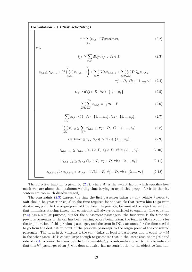
The objective function is given by (2.2), where W is the weight factor which specifies howmuch we care about the maximum waiting time (trying to avoid that people far from the citycenters are too much disadvantaged).

The constraints (2.3) express the time the first passenger taken by any vehicle j needs towait should be greater or equal to the time required for the vehicle that serves him to go fromits starting point to the origin point of this client. In practice, because of the objective functionthat minimises starting times, this constraint will always be satisfied to equality. The equation(2.4) has a similar purpose, but for the subsequent passengers: the first term is the time theprevious passenger of the car has been waiting before being taken, the term in OD

i

accounts forthe trip duration of this previous passenger, and the term in DO

i,l

accounts for the time neededto go from the destination point of the previous passenger to the origin point of the consideredpassenger. The term in M vanishes if the car j takes at least k passengers and is equal to ≠Min the other cases. M is chosen large enough to guarantee that in the latter case, the right handside of (2.4) is lower than zero, so that the variable t

j,k

is automatically set to zero to indicatethat this kth passenger of car j -who does not exist- has no contribution to the objective function.

13

The M -value should however not be too large in order to avoid complications during the linearrelaxation process1. The waiting times are non negative values as specified in (2.5). Constraints(2.6) ensure that every passengers travels one and only one time, and constraints (2.7) specifiesexpresses that each possible trip (j, k) corresponds to no more than one client. The constraints(2.8) state that if a car does not take a kth passenger, it will not take any passenger of superiorrank. Constraints (2.10) to (2.12) ensure that z

i,j,k≠1,l

is the product of the binary variablesx

i,j,k≠1

and xl,j,k

for k Ø 2.This formulation gives an idea of the complexity of the problem and of the number of related

variables (n2

p

n2

v

for the z variables only). In the rest on the report, only the VRP approaches,which are more convenient, will be used.

2.1.2 Inspiration from the Vehicle Programming ProblemInstead of seeing the services to the di�erent clients as tasks, it is tempting to use a representationof the problem that emphases more the geographical aspect. A very classical problem of discreteoptimisation that comes to the mind is the Vehicle Routing Problem, or VRP. The VRP is thegeneralisation of the Traveling Salesman Problem, or TSP with several vehicles are available: thegoal is to find the routes of vehicles (in general the number of used vehicles can be a part of theproblem) starting from one or several depots in order to visit a set of geographically scatteredpoints referred as cities with a minimum total cost (e.g. using a minimum amount of fuel orminimising the sum of the travel times). The cities can be modelled as the nodes of a graph,the routes used to link the cities being represented by the edges. The cost of the use of an edgegoing from city i to city j is represented by a the cost matrix element C

i,j

. The total cost to beminimised is classically defined as the sum of the costs of the edges that have been used by thevehicles.

For the car sharing problem, the definition of the cost matrix has to be modified. In thecase of taxis with on passenger capacity, the approach used does not consist in considering eachorigin or destination point as a city, but rather to assimilate each client to one city.

Note that the capacity of the vehicles in the framework of the VRP (which is linked to thenumber of cities that a vehicle can visit because of restrictions on the amount of merchandiseit can transport to deliver them for example), is di�erent from the capacity of the taxis of ourproblem, which is in this case of one client.

Our problem is thus similar to a VRP with the following specificities

1. The distance matrix is not symmetric: the lapse of time between arriving at the client Aorigin point and then at the client B origin point is di�erent from the time required toserve these clients in the opposite order. One can define the cost for going from client i toclient j as C

i,j

= ODi

+ DOi,j

(see Figure 2.1).

2. Since the time of service of a client is taken into account in the cost matrix, the time spentin each city is zero.

3. The capacities of our vehicles in the VRP meaning is infinite: a same vehicle can serve asmany clients as necessary.

4. The number of vehicles in use is fixed and is thus not a part of the problem.

5. There are as many depots as available vehicles. Their positions represent the initial po-sitions of the di�erent vehicles, which is formally fixed. The clients correspond to nodeswith numbers from 1 to n

p

, and the depots correspond to the nodes np

+ 1 to np

+ nv

.After dropping o� their last clients, the vehicles formally go back to their own depot, butas this last trip is not a part of the problem, one takes C

i,j

= 0 ’i œ {1, ..., np

}andj œ1In a first time, we choose M = max

i

j(dOi,j

) + np

(maxi

(ODi

+ maxi,j

(DOi,j

))

14

{np

+ 1, ..., np

+ nv

}. Besides, Ci,j

with i and j œ {np

+ 1, ..., np

+ nv

} is never used, andthus not defined. In order to simulate free starting points of the vehicles, one can replaceall the C

i,j

values (i > np

, j Æ np

) by zero, and consider that the journey of each vehiclebegins at the origin of its first client, which is then chosen optimally.

(a) Oriented graph with geographicalpoints as vertices

(b) Oriented graph with clients asvertices

Figure 2.1: Illustration of the construction of the asymmetric cost matrix used for the VRPapproach.

It is important to keep in mind that classically, a VRP with infinite capacities reduces toa TSP : if there is a cost for going back to the single depot, the minimum cost routing will beachieved by letting one single vehicle visit all the cities (see Figure 2.2).

However, in the remainder of the work, the use of the whole available fleet will be systematicas the system is expected to serve the clients as fast as possible, requiring the vehicles to servedi�erent clients simultaneously.

As a matter of fact, compared to the VRP described so far, our objective function is bedi�erent, and the fact that we consider the average or the sum of the times at which thedi�erent cities are visited has an impact on the formulation of the constraints of the problem.

For a classical VRP, one can simply define the binary variables xi,j,k

for i, j œ {1, ..., np

+nv

}and k œ {1, ..., n

v

} such that xi,j,k

= 1 i� vehicle k rides along the edge linking cities i and jand impose constraints such as continuity (if a vehicle arrives in a city, it also need to leave it),the fact that every city is visited one and only one time, and the fact that each vehicle passestrough its own depot. Considering depots as cities for which specific constraints are applied (seeconstraints (2.17) and (2.18)), the classical VRP linear integer model would be written as inFormulation2.2.

15

Formulation 2.2 (Classical VRP, 3 index version)

Minn

p

+n

vÿ

i=1

n

p

+n

vÿ

j=1

Ci,j

n

vÿ

k=1

xi,j,k

(2.13)

s.t.

n

p

+n

vÿ

i=1

n

vÿ

k=1

xi,j,k

= 1, ’j œ {1, ..., np

+ nv

} (2.14)

n

p

+n

vÿ

j=1

n

vÿ

k=1

xi,j,k

= 1, ’i œ {1, ..., np

+ nv

} (2.15)

n

p

+n

vÿ

i=1

xi,l,k

=n

p

+n

vÿ

j=1

xl,j,k

, ’l œ {1, ..., np

+ nv

}, and k œ {1, ..., nv

} (2.16)

n

p

+n

vÿ

j=1

xn

p

+k,j,k

= 1, ’k œ {1, ..., nv

} (2.17)

n

p

+n

vÿ

i=1

xi,n

p

+k,k

= 1, ’k œ {1, ..., nv

} (2.18)

xi,i,k

= 0, , ’i œ {1, ..., np

+ nv

}, and k œ {1, ..., nv

} (2.19)

ÿ

iœS

ÿ

jœS

xi,j,k

Æ |S| ≠ 1, ’S µ {1, ..., np

} : |S| Æ 2 and ’k œ {1, ..., nv

}, (2.20)

Formulation2.2,constraints (2.14) and (2.15) ensure that each city is visited one and onlyone time, constraints (2.16) ensure continuity 2 (i.e. if a vehicle k arrives at a city l, it has alsoto leave it), constraints (2.17) and (2.18) specify that each vehicle visits its own depot. Then,(2.18) constraints prevent a vehicle to stay in a city, and constraints (2.20), usually added lazilyin practice, guarantee the absence of subtours in the solution that would not pass to a depot.The VRP as it is presented here has been widely studied, and di�erent methods can be used inorder to compute either the optimal solution or approximations of these solutions. An overviewof the main methods to solve di�erent variations of this problem is presented in [15]. Anotherpossibility to avoid the use of lazy constraints is to modify the formulation by adding variablesrepresenting the times by which the cities are visited and to add constraints on these times sothat they are consistent with the chosen routes. Such a method is applied in the next paragraph,where the objective function (2.13) of the classical VRP is modified to describe the problem thiswork aims at solving.

2Note that constraint (2.16) renders the constraints set (2.14) or (2.15) redudant, as if (2.14) are satisfied,(2.15) will be automatically satisfied via (2.16) ans vice versa.

16

2.2 Problem seen as a variation of the classical VRP (the MinAvgand the MinMax problems)

In our problem however, where the maximum visit times and the average (or equivalently thesum) of these times are taken into account by the objective function, it is necessary to specifyexplicitly the time at which the cities are visited. Let t

i

denote the time after which city i isvisited, i.e. the time after which the client i is picked up by a vehicle. The objective functionreads

Minn

pÿ

i=1

ti

+ WmaxTime, (2.21)

where maxTime = maxiœ{1,...,n

p

}ti

.The variant of the VRP when only the first term of (2.21) is used is referred as a MinSum,

a MinAvg problem, or a Cumulative Capacited Vehicle Routing Problem (CCVRP)3. When theobjective function is given by maxTime only, one talks about a MinMax problem.

These alternatives to the classical VRP have been investigated only quite recently. The mainpaper introducing these two problems, exploring their di�erences with the classical VRP andproposing heuristic algorithms to solve them was written by A.M. Campbell in 2008 [8].

These problems arose in the context of delivering humanitarian aid in large zones touched bynatural disasters. In such situations, the fact that the populations obtain help quickly is moreimportant than the minimisation of the costs induced by the operation. The deliveries haveto be both fast and fair : the waiting times have to be as short as possible on average, but asleaving populations without help for a long time can be extremely damageable (one can guessthe number of causalities does not grow linearly with the waiting time), it can be sometimesinteresting to let the average waiting time slightly increase in order to lower significantly thewaiting times of the populations served in last positions.

For our optimisation of a public transport network based on the satisfaction of the clients,these objective functions are thus interesting.

Note that the concept of a minimisation of the maximum cost and / or average cost doesnot appear only in extensions of VRPs. These notions can also be used, for example, in thecontext of the Facility Location Problem. In general, there exist more sophisticated objectivefunctions than (2.21) in order to obtain fair and e�cient solutions. Ogryczak and Sliwinski [19]proposed for example to enhance the MinMax problems by minimising the average costs for thepart of the demand that su�ers from a service with the worst performances. As in our case ofthe objective function (2.21), they managed to build a set of linear constraints completing theirobjective function.

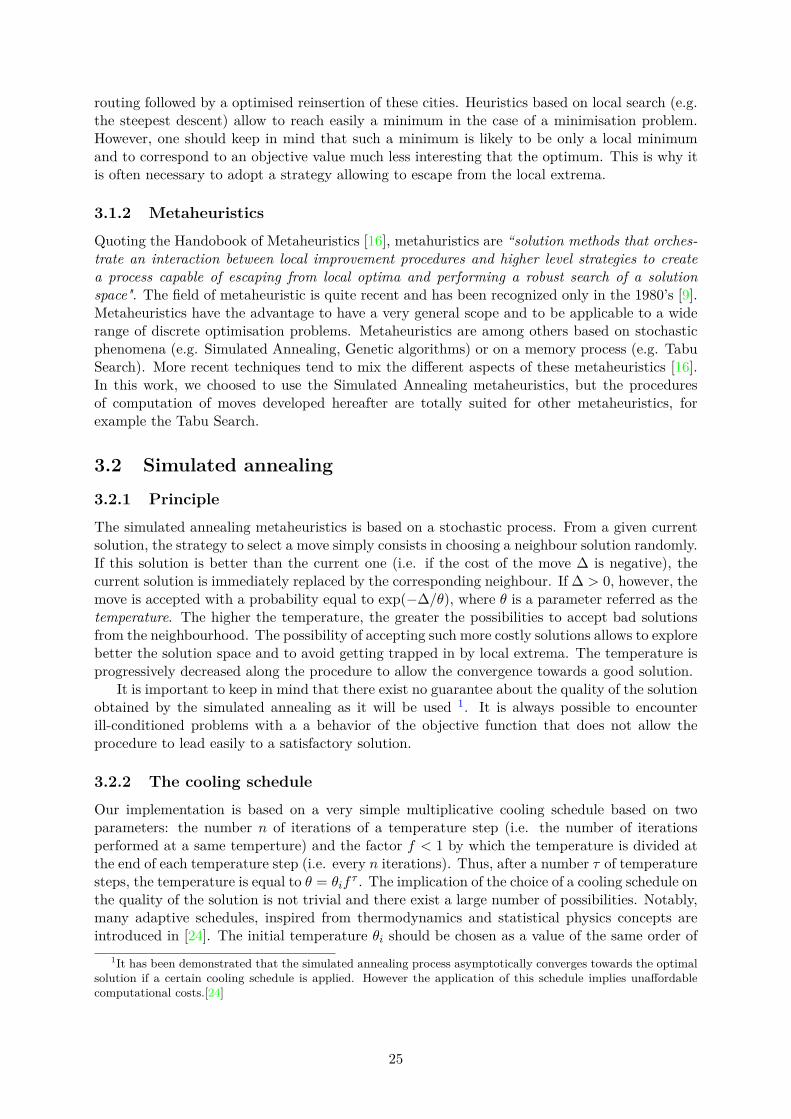
Table 2.1 compares the di�erent characteristics of the classical VRP and the two aforemen-tioned variants: the MinSum and the MinMax problem. TRP is a shorthand for TravellingRepairman Problem. It corresponds to the particular case of the MinSum VRP when only onevehicle is available.

Figure 4 presents an example that illustrates the fact that the optimal solution of a CCVRPcan be fundamentally di�erent from the one of a classical VRP.

3The word capacited is however in this case inappropriate given the infinite capacities of our vehicles in thesense of the VRP, but it is under this name that the general problem is denoted in the literature, and the notationCCVRP will thus still be used in the remainder of this text to refer to the problem with the case of W = 0

17

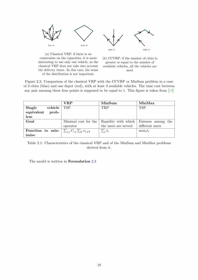
(a) Classical VRP: if there is noconstraints on the capacities, it is more

interesting to use only one vehicle, as theclassical VRP does not take into accountthe delivery times. In this case, the sense

of the distribution is not important.

(b) CCVRP: if the number of cities isgreater or equal to the number of

available vehicles, all the vehicles areused.

Figure 2.2: Comparison of the classical VRP with the CCVRP or MinSum problem in a caseof 3 cities (blue) and one depot (red), with at least 3 available vehicles. The time cost betweenany pair amonng these four points is supposed to be equal to 1. This figure is taken from [18]

VRP MinSum MinMax

Single vehicle

equivalent prob-

lem

TSP TRP TSP

Goal Minimal cost for theoperator

Rapidity with whichthe users are served

Fairness among thedi�erent users

Function to min-

imise

qi,j

Ci,j

qk

xi,j,k

qi

ti

maxi

ti

Table 2.1: Characteristics of the classical VRP and of the MinSum and MinMax problemsderived from it.

The model is written in Formulation 2.3

18

Formulation 2.3 (MinAvg-MinMax version of the VRP)

Minn

pÿ

i=1

ti

+ WmaxTime, (2.22)

s.t.

n

p

+n

vÿ

i=1

n

vÿ

k=1

xi,j,k

= 1, ’j œ {1, ..., np

+ nv

} (2.23)

n

p

+n

vÿ

j=1

n

vÿ

k=1

xi,j,k

= 1, ’i œ {1, ..., np

+ nv

} (2.24)

n

p

+n

vÿ

i=1

xi,l,k

=n

p

+n

vÿ

j=1

xl,j,k

, ’l œ {1, ..., np

+ nv

}, and k œ {1, ..., nv

} (2.25)

n

p

+n

vÿ

j=1

xn

p

+k,j,k

= 1, ’k œ {1, ..., nv

} (2.26)

xi,i,k

= 0, ’i œ {1, ..., np

+ nv

}, and k œ {1, ..., nv

} (2.27)

ti

= 0, ’i œ {np

+ 1, ..., np

+ nv

} (2.28)

tj

Ø ti

+ Ci,j

≠ (1 ≠ xi,j,k

)T, ’j œ {1, ..., np

}, i œ {1, ..., np

+ nv

} (2.29)

MaxTime Ø ti

, i œ {1, ..., np

+ nv

}. (2.30)

This formulation exhibits important di�erences with the previous one for classical VRP.Constraints (2.28) specifies that all the vehicles leave their depot at time t = 0. Constraints(2.29) reflect the fact that if a vehicle arrives at city i at time t

i

, it cannot arrive at city j (whichcannot be a depot) before time t

i

+ Ci,j

. T is a constant large enough so that in any case, ifx

i,j,k

= 0 the constraint reads tj

Ø h, with h = ti

+ Ci,j

≠ T Æ 0. In practice, if no constraintson the minimum times at which client can be served are added, constraints (2.29) are alwayssatisfied to equality because of the objective function. Constraint (2.30) is the definition of themaximum waiting time and this inequality will be tight once again because of the objectivefunction.

The trip from the last city to the depot is no more considered. As matter of fact, sincea time t

i

must be attributed to each city, the routes can no more be represented by a cycle,which is not a problem since the aforementioned trip is artificial and free of cost. This explainswhy constraint (2.18) of the VRP formulation have no equivalent in the present formulation.Furthermore, this formulation does not require subtour elimination since subtours are preventedby constraints (2.29).

19

2.3 Vehicles with capacity of more than one passenger (ridesharing)

In the case where the vehicles are allowed to carry several clients at the same time, and sincewhen a client is picked up he will not necessarily ride directly towards its destination point,there is no point in minimising the waiting time any more. Instead, the objective function isbased on thetextitarrival times, i.e. the time at which the clients are dropped at their destination point.To model once again the problem as a MinMax and MinSum inspired from the VRP, it is nownecessary go back to a graph representation where each vertex corresponds to a geographicalpoint, i.e. an origin, a destination or a depot point. In this situation, one can thus reuse theprecedent formulation with some modifications. First of all, the number of cities is now equal to2n

p

. The number of depots remains unchanged and is equal to nv

. Let us denote by P the setof origin and destination points, so that |P | = 2n

p

, and for all i œ {1, ..., |P |} define naturei

= 1if the point is an origin point, and nature

i

= ≠1 if the point is a destination point. Since onlythe arrival times are taken into account, the objective can be written

Minÿ

iœP

ti

1 ≠ naturei

2 + WmaxiœP

ti

(≠naturei

). (2.31)

Then, it is not possible to visit the di�erent cities in any order because it is always requiredto visit the origin point of a given client before visiting its destination point. Furthermore, thenumber of passengers that can be found at the same time in a same vehicle should not overcomethe vehicle capacity N

max

.If we take as a convention that the ith client with i œ {1, ..., n

p

} has for origin point i andfor destination point i + n

p

, the precedence relation constraints read

ti

Æ ti+n

p

, ’i œ {1, ..., np

}. (2.32)

The fact that a client is dropped o� at its destination point by the same vehicle as the onethat picked him up at its origin point is represented by the constraints

ÿ

jœP

xi,j,k

=ÿ

jœP

xi+n

p

,j,k

, ’i œ {1, ..., np

}, ’k œ {1, ..., nv

} (2.33)

Let now Rl,k

be the lth point visited by vehicle k œ D, except depots. The capacity con-straints can be written

Lÿ

l=1

natureR

l,k

Æ Nmax

, ’L œ {1, ..., NPointsk

}, ’k œ D (2.34)

where NPointsk

is the number of points visited by vehicle k, depot excluded.Note that the latest constraints are not written as linear programming constraints. However,

since the problem will be solved by means of metaheuristics, and not via linear programmingwhich already revealed inappropriate for the precedent problem, obtaining a complete MILPformulation is not crucial.

2.4 Adding release timesSo far, we investigated only the limit case where all the clients wan to leave their origin pointsat the same time. Relaxing this hypothese and introducing READY

i

’i œ {1, ..., np

}, which isa given of the problem denoting the time before which it is forbidden for any car to visit the

20

origin point of client i because this client is simply not ready to start its journey4. The goalis no more to minimise the arrival times of the clients, but rather the laps of time between themoment at which they want to start their journey (referred as release times) and the momentat which they arrive at destination.

The objective then reads

Minÿ

iœP

(ti

≠ READYi

)1 ≠ naturei

2 + WmaxiœP

(ti

≠ READYi

)(≠naturei

). (2.35)

Note that sinceq

iœP

READYi

is a constant, the first term of the objective function can bereduced to

qiœP

ti

1≠nature

i

2

, but it is important to keep in mind that the value of W shouldbe adapted if the same e�ect is to be obtained. The supplementary constraint is simply thatvehicles cannot arrive at origin points in advance:

ti

Ø READYi

, ’i œ {1, ..., np

}. (2.36)

2.5 Towards more fairnessUntil now, the quantities that were systematically minimised for each client were totally in-dependent of the length of the distance between the origin and the destination point of thisclient. The idea is to consider that a situation where a client requiring a short trip and a clientrequiring a long trip encounter similar waiting/arrival times is not fair. Figure 2.3a illustrates acase where the maximum relative arrival times are automatically minimised by solving the carsharing problem with a minimisation of the maximum absolute arrival time, while it is not thecase in the configuration of Figure 2.3b. For this second configuration, the route O

2

, O1

, D1

, D2

gives arrival times of 32 and 62 for clients 1 and 2 respectively, i.e. relative arrival times of16 and 3.1. On the other hand, for the route O

2

, D2

, O1

, D1

, the arrival times are 52 and 20(smaller average and maximum than with the previous route), but there is a prohibitive (more)prohibitive relative arrival time of 26 for client 21. Using the objective function

Minÿ

iœP

ti

1 ≠ naturei

2 + Wrel

maxiœP

ti

Ci,i+n

p

(≠naturei

), (2.37)

with Wrel

chosen consistently, which minimises the maximum relative arrival times in thiscase, allows the system to chose more fair solutions with respect to this length of required journeywhen it is possible.

4The release times are added to the ride sharing problem in this section, but they could without any problembe added to the car sharing problem.

21

(a) The client with a small trip demandis naturally advantaged by objectivefunctions on absolute waiting/arrival

time.

(b) The client with a small trip demandis served after the one with long trip

except if the objective function takes intoaccount relative waiting/arrival times.

Figure 2.3: Illustration of the relevance of the objective functions including relative arrivaltimes.

22

Chapter 3

Methodology of resolution

In this Chapter, we first recall the principles of local search procedure and of metheuristicsthat are used to solve discrete optimisation problems for which it is not possible to obtain theoptimal solution within a reasonable time with an exact algorithm such as the Branch and Boundalgorithm used in most of the linear solvers. We then set the focus on a Simulated Annealingmetaheuristics, and after having described this method and presented its parameters, we describea simple local search procedure suited to the problems described in Chapter 2. This local searchprocedure is then embedded in the Simulated Annealing procedure and measurements of thee�ciency of the obtained algorithm are then performed in terms of both the execution time andthe reached value of the objective function. The last section of this chapter is devoted to avenuesfor improving the performances of the procedure.

3.1 Local search and metaheuristicsIt is well known that solving NP-hard problems as the Travelling Salesman Problem or theclassical Vehicle Routing Problem is very challenging. However, such problems can be solvedto optimality in a reasonable time for moderate instance sizes. For example, a simple linearproblem formulation of the TSP was experimented using the Gurobi solver [2] for an instanceof 50 cities, and the optimal solution was obtained within 3 seconds. On the contrary, for theTRP (Traveling Repairman Problem), which can be modelled with exactly the same formulationas the TSP except that the objective function involves more variables, 67 seconds were necessaryto obtain the optimal solution for an instance of 10 cities only. For solving classical TSP or VRPfor large instances or MinSum and MinMax problems even for small instances, people have toabandon exact algorithms and use heuristic and meta-heuristic approaches instead.

3.1.1 Solution space and local search.The solution space of a problem represents the set of its (feasible) solutions. For the problemsdescribed in Chapter 2, a solution correspond to a valid set of routings for the di�erent vehicles.It is interesting to have an idea of the size of the solution space as a function of the size of ourdemand-based public transit system problem. The considerations that follow are based on thecar-sharing problem (one client per city or point). They could be expanded to the ride sharingproblem by multiplying the number of cities or points by 2, but one should then also take intoaccount the practical restrictions on the routes (visiting the origin point of a client before theirdestination and respecting the vehicles capacity).

In the car-sharing problem, let us consider an ideal situation where the clients are evenlydistributed among the vehicles, i.e. where each vehicle serves an equal number r = n

p

/nv

ofclients. First of all, let us compute the number of possible ways to distribute the di�erentpassengers among the vehicles, without considering the order in which they are served. There

23

np

log10

(—) log10

(“)10.0 0 13.1220.0 3.0103 24.94630.0 7.7815 38.98340.0 13.802 54.47150.0 20.792 71.04360.0 28.573 88.4870.0 37.024 106.6480.0 46.055 125.4190.0 55.598 144.73100.0 65.598 164.53

Table 3.1: Values of the di�erent factors of the number possible solutions function given by(3.1) as a function of n

p

and nv

for the car-sharing problem.

are Cn

p

r

ways of filling a first vehicle with r clients among np

. For each of these possibilities,there are C

n

p

≠r

r

ways to fill a second vehicle, and so on and so forth. If for a group of clientstravelling in the same vehicle, the fact that they are served by a vehicle A or a vehicle B isimportant (e.g. because it is considered that each vehicle starts its route from a di�erent givendepot point), then the number of possible configurations is multiplied by n

v

!. Then, for a givendistribution of the clients among the vehicles, there are (r!)n

v di�erent permutations possible(n

v

! for each vehicle). The total number of possibilities is given by

nsol

(np

, nv

) = nv

!¸˚˙˝–

(r!)n

v

¸ ˚˙ ˝—

n

v

≠1Ÿ

m=0

Cn

p

≠rm

r

¸ ˚˙ ˝“

. (3.1)

Table 3.1 shows some values of the factors that compose nsol

for a couple of np

and nv

values.Naturally, the real size of the solution space is much larger, as only the cases where the clientsare evenly distributed among the vehicles are considered by equation (3.1) in order to give anidea.

Most of the approximation algorithms (heuristics and metaheuristics) are based on the localsearch concept. The basic idea is, starting from a solution, to browse the solution space stepby step, following a given strategy in the hope to converge towards the best solution possible.Naturally, only a small part of the space solution is visited. Practically, from a given solution,it is possible to go to another one if it belongs to the neighbourhood of this solution, i.e. if itis reachable by performing one single move. For a classical VRP problem, the moves proposedby Osman in [20] simply consist in either removing a city from the route of a vehicle and toinsert it somewhere in the route of another (or the same) vehicle or to interchange the positionof two cities in the lists of cities to be visited by the vehicles. This neighbourhood definition andsome variations for the ride sharing problem are used in the implementation of our optimisationsystem described in the next sections.

The idea is to be able to compute the cost related to a move as fast as possible, as thisoperation is to be performed a large number of times in order to get a solution as reliable aspossible. The aforementioned strategies consist in choosing which kind of moves are performed(e.g. browsing the whole neighbourhood and choosing the best move,...) and what is thesubsequent action (e.g. updating the solution according to a move only if it improves theobjectives,...). Note that the notion of move and neighbourhood is very general. For example,Shawn developed for example a large neighbourhood search procedure for the classical VRP[21]. In his procedure, a move consists in the removal of a set of cities from the current solution

24

routing followed by a optimised reinsertion of these cities. Heuristics based on local search (e.g.the steepest descent) allow to reach easily a minimum in the case of a minimisation problem.However, one should keep in mind that such a minimum is likely to be only a local minimumand to correspond to an objective value much less interesting that the optimum. This is why itis often necessary to adopt a strategy allowing to escape from the local extrema.

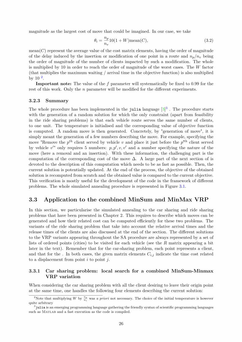
3.1.2 MetaheuristicsQuoting the Handobook of Metaheuristics [16], metahuristics are “solution methods that orches-trate an interaction between local improvement procedures and higher level strategies to createa process capable of escaping from local optima and performing a robust search of a solutionspace". The field of metaheuristic is quite recent and has been recognized only in the 1980’s [9].Metaheuristics have the advantage to have a very general scope and to be applicable to a widerange of discrete optimisation problems. Metaheuristics are among others based on stochasticphenomena (e.g. Simulated Annealing, Genetic algorithms) or on a memory process (e.g. TabuSearch). More recent techniques tend to mix the di�erent aspects of these metaheuristics [16].In this work, we choosed to use the Simulated Annealing metaheuristics, but the proceduresof computation of moves developed hereafter are totally suited for other metaheuristics, forexample the Tabu Search.

3.2 Simulated annealing3.2.1 PrincipleThe simulated annealing metaheuristics is based on a stochastic process. From a given currentsolution, the strategy to select a move simply consists in choosing a neighbour solution randomly.If this solution is better than the current one (i.e. if the cost of the move � is negative), thecurrent solution is immediately replaced by the corresponding neighbour. If � > 0, however, themove is accepted with a probability equal to exp(≠�/◊), where ◊ is a parameter referred as thetemperature. The higher the temperature, the greater the possibilities to accept bad solutionsfrom the neighbourhood. The possibility of accepting such more costly solutions allows to explorebetter the solution space and to avoid getting trapped in by local extrema. The temperature isprogressively decreased along the procedure to allow the convergence towards a good solution.

It is important to keep in mind that there exist no guarantee about the quality of the solutionobtained by the simulated annealing as it will be used 1. It is always possible to encounterill-conditioned problems with a a behavior of the objective function that does not allow theprocedure to lead easily to a satisfactory solution.

3.2.2 The cooling scheduleOur implementation is based on a very simple multiplicative cooling schedule based on twoparameters: the number n of iterations of a temperature step (i.e. the number of iterationsperformed at a same temperture) and the factor f < 1 by which the temperature is divided atthe end of each temperature step (i.e. every n iterations). Thus, after a number · of temperaturesteps, the temperature is equal to ◊ = ◊

i

f · . The implication of the choice of a cooling schedule onthe quality of the solution is not trivial and there exist a large number of possibilities. Notably,many adaptive schedules, inspired from thermodynamics and statistical physics concepts areintroduced in [24]. The initial temperature ◊

i

should be chosen as a value of the same order of1It has been demonstrated that the simulated annealing process asymptotically converges towards the optimal

solution if a certain cooling schedule is applied. However the application of this schedule implies una�ordablecomputational costs.[24]

25

magnitude as the largest cost of move that could be imagined. In our case, we take

◊i

= np

nv

10(1 + W )mean(C), (3.2)

mean(C) represent the average value of the cost matrix elements, having the order of magnitudeof the delay induced by the insertion or modification of one point in a route and n

p

/nv

beingthe order of magnitude of the number of clients impacted by such a modification. The wholeis multiplied by 10 in order to reach the order of magnitude of the worst cases. The W factor(that multiplies the maximum waiting / arrival time in the objective function) is also multipliedby 10 2.

Important note: The value of the f parameter will systematically be fixed to 0.99 for therest of this work. Only the n parameter will be modified for the di�erent experiments.

3.2.3 SummaryThe whole procedure has been implemented in the julia language [3]3 . The procedure startswith the generation of a random solution for which the only constraint (apart from feasibilityin the ride sharing problems) is that each vehicle route serves the same number of clients,to one unit. The temperature is initialised and the corresponding value of objective functionis computed. A random move is then generated. Concretely, by "generation of move", it issimply meant the generation of a few numbers describing the move. For example, specifying themove "Remove the pth client served by vehicle v and place it just before the pÕth client servedby vehicle vÕ" only requires 5 numbers: p, pÕ, v, vÕ and a number specifying the nature of themove (here a removal and an insertion). With these information, the challenging part is thecomputation of the corresponding cost of the move �. A large part of the next section of isdevoted to the description of this computation which needs to be as fast as possible. Then, thecurrent solution is potentially updated. At the end of the process, the objective of the obtainedsolution is recomputed from scratch and the obtained value is compared to the current objective.This verification is mostly useful for the development of the code in the framework of di�erentproblems. The whole simulated annealing procedure is represented in Figure 3.1.

3.3 Application to the combined MinSum and MinMax VRPIn this section, we particularise the simulated annealing to the car sharing and ride sharingproblems that have been presented in Chapter 2. This requires to describe which moves can begenerated and how their related cost can be computed e�ciently for these two problems. Thevariants of the ride sharing problem that take into account the relative arrival times and therelease times of the clients are also discussed at the end of the section. The di�erent solutionsto the VRP variants appearing throughout the SA procedure are always represented by a set oflists of ordered points (cities) to be visited for each vehicle (see the R matrix appearing a bitlater in the text). Remember that for the car-sharing problem, each point represents a client,and that for the . In both cases, the given matrix elements C

i,j

indicate the time cost relatedto a displacement from point i to point j.

3.3.1 Car sharing problem: local search for a combined MinSum-MinmaxVRP variation

When considering the car sharing problem with all the client desiring to leave their origin pointat the same time, one handles the following four elements describing the current solution:

2Note that multiplying W by np

nvwas a priori not necessary. The choice of the initial temperature is however

quite arbitrary3julia is an emerging programming language gathering the friendly syntax of scientific programming languages

such as Matlab and a fast execution as the code is compiled.

26

Figure 3.1: Flow chart representing the adopted simulated annealing procedure. obj representsthe current value of the objective and cpt and iteration counter.

• R, the routes matrix. For nv

= 2 and np

= 5, an example of this matrix is given by

R =A

6 2 3 4 6 0 0 07 1 5 7 0 0 0 0

B

where the numbers 1 to np

refer to client points and the numbers np

+ 1 to np

+ nv

referto depots points (here 6 and 7)

• The times by which these points are visited: tk,i

is the time at which point Rk,i

is visited.The times of visit of the depots are always set to zero. For the aforementioned R matrix,one can have 4

t =A

0 2 6 23 0 0 0 00 2 7 0 0 0 0 0

B

• A vector with the number of clients served by each vehicle. In order to be able to keepthe same notation when considering VRP variations where cities represent geographicalpoints and not clients, this vector is called nb_points. The depots being excluded fromthe counting of visited points, for the mentioned R example, one has

nb_points =13 2

2

.

• The maximum departure times of the clients are given by the vector

maxTimes =123 7

2

4Note that the fact that the elements of the second column of t are di�erent from zero indicates that werepresent a problem where the depots are assumed to be prealably fixed.

27

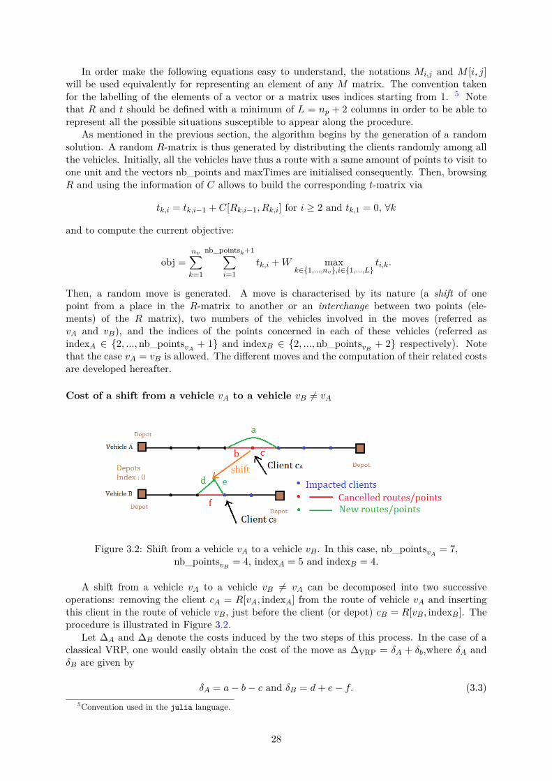
In order make the following equations easy to understand, the notations Mi,j

and M [i, j]will be used equivalently for representing an element of any M matrix. The convention takenfor the labelling of the elements of a vector or a matrix uses indices starting from 1. 5 Notethat R and t should be defined with a minimum of L = n

p

+ 2 columns in order to be able torepresent all the possible situations susceptible to appear along the procedure.

As mentioned in the previous section, the algorithm begins by the generation of a randomsolution. A random R-matrix is thus generated by distributing the clients randomly among allthe vehicles. Initially, all the vehicles have thus a route with a same amount of points to visit toone unit and the vectors nb_points and maxTimes are initialised consequently. Then, browsingR and using the information of C allows to build the corresponding t-matrix via

tk,i

= tk,i≠1

+ C[Rk,i≠1

, Rk,i

] for i Ø 2 and tk,1

= 0, ’k

and to compute the current objective:

obj =n

vÿ

k=1

nb_points

k

+1ÿ

i=1

tk,i

+ W maxkœ{1,...,n

v

},iœ{1,...,L}ti,k

.

Then, a random move is generated. A move is characterised by its nature (a shift of onepoint from a place in the R-matrix to another or an interchange between two points (ele-ments) of the R matrix), two numbers of the vehicles involved in the moves (referred asv

A

and vB

), and the indices of the points concerned in each of these vehicles (referred asindex

A

œ {2, ..., nb_pointsv

A

+ 1} and indexB

œ {2, ..., nb_pointsv

B

+ 2} respectively). Notethat the case v

A

= vB

is allowed. The di�erent moves and the computation of their related costsare developed hereafter.

Cost of a shift from a vehicle vA

to a vehicle vB

”= vA

Figure 3.2: Shift from a vehicle vA

to a vehicle vB

. In this case, nb_pointsv

A

= 7,nb_points

v

B

= 4, indexA

= 5 and indexB

= 4.

A shift from a vehicle vA

to a vehicle vB

”= vA

can be decomposed into two successiveoperations: removing the client c

A

= R[vA

, indexA

] from the route of vehicle vA

and insertingthis client in the route of vehicle v

B

, just before the client (or depot) cB

= R[vB

, indexB

]. Theprocedure is illustrated in Figure 3.2.

Let �A

and �B

denote the costs induced by the two steps of this process. In the case of aclassical VRP, one would easily obtain the cost of the move as �

VRP

= ”A

+ ”b

,where ”A

and”

B

are given by

”A

= a ≠ b ≠ c and ”B

= d + e ≠ f. (3.3)5Convention used in the julia language.

28

In equations (3.3), a, b, c, d, e and f refer to the costs indicated in Figure 3.2 with amongothers a = C[R[v

A

, indexA

≠ 1], R[vA

, indexA

+ 1]] and e = C[R[vA

, indexA

≠ 1], R[vB

, indexB

]].However, given the objective function of the combined MinSum MinMax problem, the modi-

fication of the times at which the clients are served after the shift should be taken into account,and finally, one obtains

�A

= (nb_pointsvA

≠ indexA

+ 1)¸ ˚˙ ˝

number of clients impacted by the removal

”A

≠ t[vA

, indexA

]¸ ˚˙ ˝

waiting time of the removed client

(3.4)

and

�B

= (nb_pointsvB

≠ indexB

+ 2)¸ ˚˙ ˝

number of clients impacted by the insertion

”B

+ t[vB

, indexB

] + C[R[vB

, indexB

≠ 1], R[vA

, indexA

]]¸ ˚˙ ˝

waiting time of the inserted client

.

(3.5)These �

A

and �B

values do not take into account the potential variation of the maximumvisiting time. Defining newMax

A

= maxTimesvA

+ ”A

and newMaxB

= maxTimesvB

+ ”B

, ifnewMax is the maximum value among maxTimes

k

, k œ {1, ..., nv

}\{vA

, vB

},one can write

� = �a

+ �b

+ W (newMax ≠ maxkœ{1,...,n

v

}maxTimes). (3.6)

Cost of a shift inside a vehicle route

Figure 3.3: Shift inside the vehicle vA

= vB

. In this case, nb_pointsv

A

= 7,indexA

= 6 andindex

B

= 4. 4 clients are impacted by the insertion.

When vA

= vB

, it can be trivially found that if indexA

= indexB

or if indexA

= indexB

≠ 1,there is no move to be observed. In the other cases, the cost for removing the client from theirinitial position is computed the same way as previously with equation (3.4). Computing ”

b

thesame way as previously, �

B

can be obtained by multiplying ”B

by the number of clients impactedby the insertion of the client, which is equal to nb_points

B

≠ indexB

+1 if indexB

< indexA

andto nb_points

B

≠ indexB

+ 2 if indexB

> indexA

+ 1. The former case is illustrated in Figure 3.3..

Cost of an interchange between two di�erent vehicles

An interchange move simply consists in switching two points (except depots) from the R matrix.An interchange move can thus either happen for two clients served by di�erent vehicles or twoclients served by the same vehicle.

An interchange between two clients from vehicles vA

and vB

”= vA

is illustrated in Figure3.4. Here, the di�erence in the waiting times of the clients served after the changes are given by

”A

= a + b ≠ c ≠ d and ”B

= e + f ≠ g ≠ h, (3.7)

where a = C[R[vA, indexA

≠ 1], R[vB, indexB

]],etc.

29

Figure 3.4: Interchange between the vehicles vA

andvB

”= vA

. In this case,nb_points

v

A

= nb_pointsv

A

= 5,indexA

= 4 and indexB

= 3.

With a reasoning similar to previously, one gets

�A

= ”A

(nb_pointsv

A

≠ indexA

+ 1) ≠ t[vA

, indexA

] + t[vA

, indexA

≠ 1] + a (3.8)

and

�B

= ”B

(nb_pointsv

B

≠ indexB

+ 1) ≠ t[vB

, indexB

] + t[vB

, indexB

≠ 1] + e. (3.9)

Cost of an interchange inside a vehicle

Figure 3.5: Interchange inside the vehicle vA

. nb_pointsv

A

= 8, indexA

= 3 and indexB

= 7.

The advantage of equations (3.8) and (3.9) is that they are still valid when vA

= vB

, in thecase where |index

A

≠ indexB

| > 1. As shown in the example presented in Figure 3.5, ”A

and ”b

can be computed with equations (3.7) and the number of clients impacted by both the routeschanges is given by nb_points

v

A

≠ indexA or B

+ 1In the case where the clients to be interchanged are neighbour, i.e. if index

B

= indexB

+ 1,one can simply compute

”AB

= ≠C[R[vA

, indexA

≠ 1], R[vA

, indexA

]] ≠ C[R[vA

, indexA

], R[vA

, indexB

]]≠ C[R[v

A

, indexB

], R[vA

, indexB

+ 1]] + C[R[vA

, indexA

≠ 1], R[vA

, indexB

]]+ C[R[v

A

, indexB

], R[vA

, indexA

]] + C[R[vA

, indexA

], R[vA

, indexB

+ 1]] (3.10)

which impacts nb_pointsv

A

≠ indexB

+ 1 clients.The treatment of the maximum times happens exactly as in the case of a shift move (equation

3.6) to obtain �.If any of the moves presented so far is accepted, (i.e. if � < 0 or exp(≠�/◊) > ⁄, ⁄ being

a random parameter with an uniform distribution between 0 and 1), the appropriate lines of Rand t are uploaded, as well as nb_points and maxTimes.

30

3.3.2 Ride sharing problem with maximum arrival timesWhen considering the possibility to put several clients together in a same vehicle, it is necessaryto consider, in the VRP variant problem, a number of cities equal to twice the number of clients(one origin and one destination point by client). In this problem, the clients are still numberedfrom 1 to n

p

, but the number of non-depots points is equal to 2np

. The origin points of a clientc is labelled point c, and his destination point is labelled N

p

+ c. The depot of the kth vehicle isa point that is labelled 2n

p

+ k. However, in order to make the reading of the routes easier, thedestination points of client c will be written as ≠c. An example of a R matrix for this problemwith n

p

= 5 and nv

= 2 is given by

R =A

11 +1 +4 ≠1 +2 ≠4 ≠2 11 0 012 +3 +5 ≠3 ≠5 12 0 0 0 0

B

The t matrix plays the same role as in the previous problem, as well as maxTimes and nb_points,with nb_points

k

representing twice the number of clients on the route of vehicle k. To solve theproblem, it is necessary to introduce some new matrices. Their example values are consistentwith the routes presented in the latest R matrix.

• The Out matrix that shows at which points clients are getting out of a vehicle. It will beuseful when computing the objective variations since only the times by which the clientsget out the vehicle are taken into account in the objective function.

Out =A

0 0 0 1 0 1 1 0 0 00 0 0 1 1 0 0 0 0 0

B

(3.11)

• The INDEX matrix, which contains the information about the positions in the R matrixwhere the origin points (col 1) and the destination points of a client can be found (withoutspecifying the car):

INDEX =

Q

ccccca

2 45 72 43 63 5

R

dddddb(3.12)

• The population matrix: Pop[k, i] denotes the number of clients on board of vehicle k whenit leaves the ith point of its route. It is used in order to check if the proposed moves arefeasible.

Pop =A

0 1 2 1 2 1 0 0 0 00 1 2 1 0 0 0 0 0 0

B

(3.13)

The value of the objective function can be computed as

obj =n

aÿ

k=1

nb_points

k

+1ÿ

i=1

tk,i

Outk,i

+ W maxkœ{1,...,n

p

}t[k, nb_points

k

+ 1] (3.14)

A simulated annealing iteration begins with the choice of a feasible move, i.e. a move thatdoes not lead to a situation where at a given moment, the number of passengers inside a vehicleexceeds the capacity N

max

. For this problem, moving one client corresponds to moving twopoints in the routes of the vehicles: the origin and the destination point of the client. As forthe previous problem, the specification of a move consists in its nature (shift or interchange),the two implicated vehicles v

A

and vB

and the positions of the concerned clients in the vehicleslist of point. For interchanges and for the removal of a client from a vehicle, it is su�cient to

31

chose a random number in {2, ..., nb_pointsk

+ 1} for the considered vehicle k. If this numbercorresponds to an origin (resp. a destination point), the position of the destination (resp.origin)point can be retrieved from the INDEX matrix. The origin and destination indices are referredas index

v

A

,in

and indexv

A

,out

respectively. In the case of an interchange 6, a client should bechosen the same way in the second vehicle. In the case of a shift, in the vehicle where the clientwill be inserted, it is necessary to chose two random numbers: index

v

B

,in

and indexv

B

,out

, whichcorrespond respectively to the positions in vehicle v

B

before which the origin point and thedestination point of the client coming from vehicle v

A

is to be inserted. These two value shouldbe chosen in {1, ..., nb_points

v

B

+ 2} with indexv

B

,in

Æ indexv

B

,out

. If the choice of these twovalue does not lead to a feasible move, they are chosen again until obtaining a valid combination.Once a feasible move is determined, the corresponding move cost � can be computed.

Cost of a shift

As for the former problem, one computes successively the cost due to the removal of the clientfrom the vehicle v

A

and the cost of the insertion of the client in vehicle vB

. In the currentversion of the software, when v

A

= vB

, a copy of the rows of the vth

A

line of R, t, Pop and Out isdone. The removal of the client is performed on these copies, so that if the computation of thecost due to the reinsertion of the client can then be performed with the same formula as whenv

A

”= vB

. In this case, indexv

B

,in

and indexv

B,out

are chosen in {1, ..., nb_pointsv

B

}. 7

Figure 3.6: Shift move with nb_pointsv

A

= 8, nb_pointsv

A

= 6, indexvA,in

= 4, indexvA,in

=4, index

v

A

,in

= 3, indexv

A

,out

= 7, indexv

B

,in

= 4, indexv

B

,out

= 6 .

Figure 3.6 shows an example of a shift move. One can compute ”A,in

= a ≠ b ≠ c, ”A,out

=d ≠ e ≠ f, ”

B,in

= g + h ≠ i and ”B,out

= j + k ≠ l. For example, a is computed as a =C[SIN(R[v

A

, indexv

A

,in

≠ 1]), SIN(R[vA

, indexv

A

,in

≠ 1])], where ’z < 0, SIN(z) = ≠z + np

and’z Ø, SIN(z) = z. Note that SIN stands for Shift If Negative. The number of arrival timesimpacted by these di�erent changes of route (not to be confused with the number of impactedpoints) are computed using the Out matrix, which allow to obtain the variations of the objectivefunction (maximum arrival time considerations excluded) in both vehicles as 8

6For the seek of simplicity, the interchanges within a given vehicle route are forbidden. They can however stillbe performed by a series of shift moves. This reduction of the neighbourhood is expected to have only a negligibleimpact on the solution.

7Note that this approach avoids complicated computations but is susceptible to slow down the process.8The ’-1’ in equation (3.15) allows not to take the removed destination point into account.

32

�A

= ”A,in

Q

anb_points

v

A

+1ÿ

i=index

v

A

,in

+1

Out[vA

, i] ≠ 1

R

b

¸ ˚˙ ˝Number of arrival times impacted by the removal of the client origin point

+

”A,out

Q

anb_points

v

A

+1ÿ

i=index

v

A

,in

+1

Out[vA

, i]

R

b

¸ ˚˙ ˝Number of arrival times impacted by the removal of the client destination point

(3.15)

and similarly 9

�B

= ”B,in

Q

anb_points

v

B

+1ÿ

i=index

v

B

,in

Out[vB

, i] + 1

R

b

¸ ˚˙ ˝Number of arrival times impacted by the insertion of the client origin point

+

”A,out

Q

anb_points

v

B

+1ÿ

i=index

v

B

,out

Out[vB

, i]

R

b

¸ ˚˙ ˝Number of arrival times impacted by the insertion of the client destination point

. (3.16)

The maximum times can be handled in a way similar to the former problem, since the lastpoint before going back always corresponds to the destination point of the last client.

Note that for all the configurations met, if indexv

.

,out

= indexv

A

/B,in

+ 1 for a removal oran exchange, or if index

v

A

/B,out

= indexv

A

/B,in

for an insertion, one consider only a local cost”

A/B,in&out

impacting the points from indexv

A/B

,out

+ 1 to nb_pointsv

A/B

≠1

.

Cost of an interchange

In the case of an interchange, the computation of ”A,in

, ”A,in

, ”B,in

and ”B,in

can be done byreasoning as in the previous cases, and the number of impacted arrival times can be computedby browsing each time the Out matrix between indices index

A/B,in/out

+ 1 to nb_points + 1 ,no’+1’ or ’-1’ needing to be added in any case.

3.3.3 Ride sharing with maximum relative arrival timeWith trip

i

denoting the time required to travel directly from the origin to the destination pointof client i, the objective can be computed as

obj =n

aÿ

k=1

nb_points

k

+1ÿ

i=1

tk,i

Outk,i

+ Wrel

maxkœ{1,...,n

p

},iœ{1,...,L}

At[k, i]

tripR[k,i]

Out[k, i]B

. (3.17)

The main drawback of this objective function is that this time, when performing a move, thecost relative the variation of the considered maximum for the route of a given vehicle is nomore equal to ”

v

A/B

,in

+ ”v

A/B

,out

, which as the case for the absolute arrival times. The movesconsidered are exactly the same as in the previous problem. A simple version implementationwas constructed was implemented by computing an update of the solution whatever the cost ofthe move and then re-computing this cost from scratch in order to obtain �. This high-costprocedure leads to long computation times, and there are possibilities of ameliorations to beexplored.

9The ’+1’ in equation (3.16) allows to take the inserted destination point into account.

33

3.3.4 Multi-passengers vehicles with release timesThe current version of the software allows to solve the ride sharing problem with the followingMinSum objective function:

2n

pÿ

i=n

p

+1

(ti

≠ READYi

), (3.18)

defining the release time READYi

as the time at which client i œ {1, ..., np

} is ready to leavetheir origin point. Instead of considering that the cases where a vehicle arrives at the origin pointof a client who is not ready yet are infeasible, we simply assign a cost to the sum of such advancetimes. This approach allows to reuse most of the functionalities developed for solving the ridesharing problem, and it also allows to study the potential modifications on the behaviour andthe performances of the ride sharing system when modifying the weight W

adv

attributed to suchadvance times in the objective function (see Chapter 4). The problems can thus be translatedin the minimisation of

2n

pÿ

i=n

p

+1

ti

+ Wadv

ÿ

i=n

p

+1

ADVi

H(ADVi

) (3.19)

with ADVi

= READYi

≠ ti

, H(x) = 1 if x Ø 0 and H(x) = 0 if x < 0. A solution could befor example given by

R =A

11 +1 +4 ≠1 +2 ≠4 ≠2 11 0 012 +3 +5 ≠3 ≠5 12 0 0 0 0

B

t =A

0 3 10 14 20 23 25 0 0 00 2 8 12 13 0 0 0 0 0

B

ADV =12 5 ≠10 5 2

2.

The solution is feasible in the sense of the release times set as constraints in the cases whereall the elements of the ADV vector are negative. The used algorithm is identical to the ridesharing problem with absolute times, except that in order to compute the cost � associated toa move, one should add to �

A

and �B

a penalty of Wadv

times the total di�erence of ’positiveadvances’. The idea is to sum up the individual penalties for all the clients in a vehicle routethat follow a removal, insertion or interchange. The penalty is computed for each client i on thebasis on the change of departure time ”

A/B,in

or ”A/B,in

+ ”A/B,out

, the value of Wadv

,the initialand the new value of ADV

i

. The operation performed with these two values being dependantof their sign in order to compute the variation of the product W

adv

ADVi

H(ADVi

).

3.4 Performances of the methodIn order to use the algorithms described in the previous section in a wise way, it is important toknow, given the problem parameters, how long the program should run to obtain a good qualitysolution. This amounts to know on one hand how long the iterations during the simulatedannealing procedure last, and on the other hand, how many of these iterations are necessary toreach solutions considered as good.

3.4.1 Computation timesWe now give a quantification of the rapidity with which the � evaluation and the potentialupdate of the data are performed as a function of the size of the problem. Therefore, we run 10

10The executions of the code are performed on the THALES machine which has the following specifications: CPU : Intel Core i7-990X at 3.47GHz, 6 cores, 12 threads; RAM : DDR3-1333 SDRAM (24Gb). All the

34

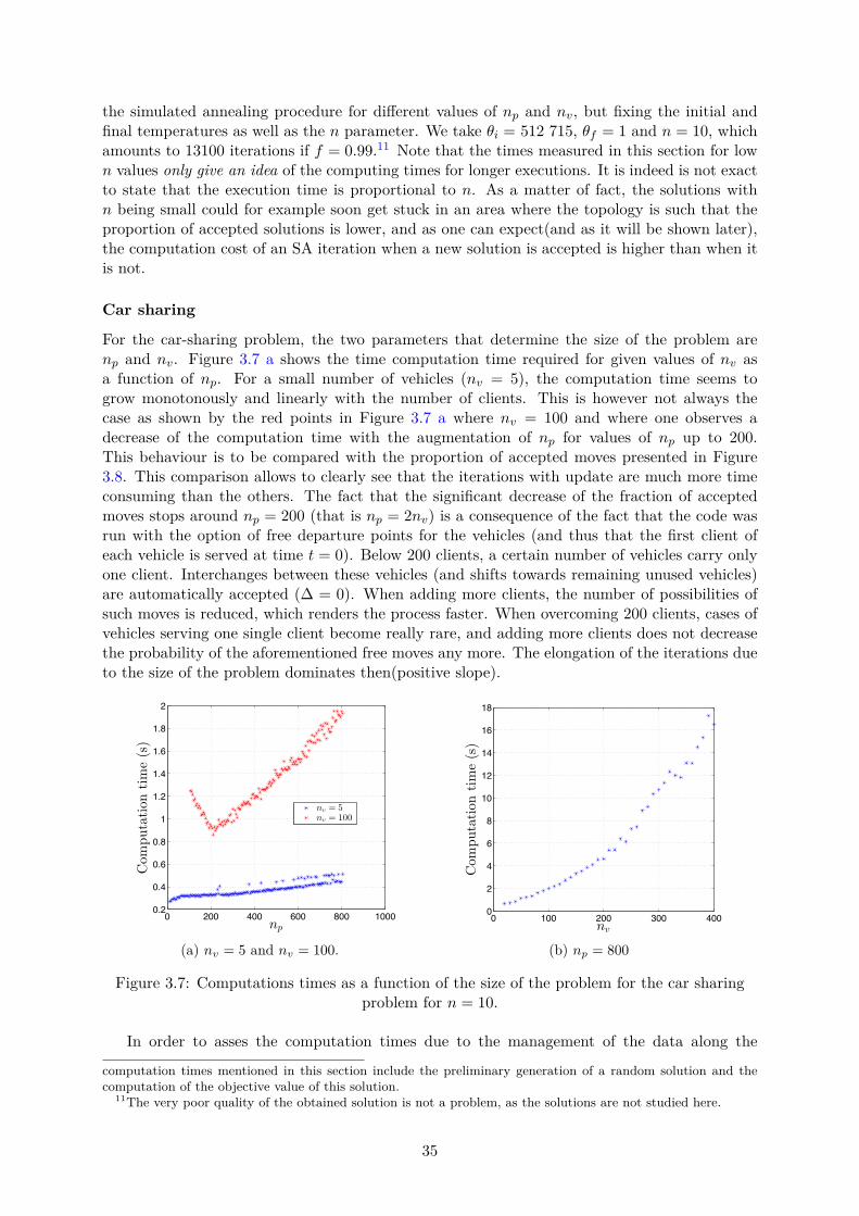
the simulated annealing procedure for di�erent values of np

and nv

, but fixing the initial andfinal temperatures as well as the n parameter. We take ◊

i

= 512 715, ◊f

= 1 and n = 10, whichamounts to 13100 iterations if f = 0.99.11 Note that the times measured in this section for lown values only give an idea of the computing times for longer executions. It is indeed is not exactto state that the execution time is proportional to n. As a matter of fact, the solutions withn being small could for example soon get stuck in an area where the topology is such that theproportion of accepted solutions is lower, and as one can expect(and as it will be shown later),the computation cost of an SA iteration when a new solution is accepted is higher than when itis not.

Car sharing

For the car-sharing problem, the two parameters that determine the size of the problem aren

p

and nv

. Figure 3.7 a shows the time computation time required for given values of nv

asa function of n

p

. For a small number of vehicles (nv

= 5), the computation time seems togrow monotonously and linearly with the number of clients. This is however not always thecase as shown by the red points in Figure 3.7 a where n

v

= 100 and where one observes adecrease of the computation time with the augmentation of n

p

for values of np

up to 200.This behaviour is to be compared with the proportion of accepted moves presented in Figure3.8. This comparison allows to clearly see that the iterations with update are much more timeconsuming than the others. The fact that the significant decrease of the fraction of acceptedmoves stops around n

p

= 200 (that is np

= 2nv

) is a consequence of the fact that the code wasrun with the option of free departure points for the vehicles (and thus that the first client ofeach vehicle is served at time t = 0). Below 200 clients, a certain number of vehicles carry onlyone client. Interchanges between these vehicles (and shifts towards remaining unused vehicles)are automatically accepted (� = 0). When adding more clients, the number of possibilities ofsuch moves is reduced, which renders the process faster. When overcoming 200 clients, cases ofvehicles serving one single client become really rare, and adding more clients does not decreasethe probability of the aforementioned free moves any more. The elongation of the iterations dueto the size of the problem dominates then(positive slope).

0 200 400 600 800 10000.2

0.4

0.6

0.8

1

1.2

1.4

1.6

1.8

2

np

Com

putation

time(s)

nv = 5nv = 100

(a) nv = 5 and nv = 100.

0 100 200 300 4000

2

4

6

8

10

12

14

16

18

nv

Com

putation

time(s)

(b) np = 800

Figure 3.7: Computations times as a function of the size of the problem for the car sharingproblem for n = 10.

In order to asses the computation times due to the management of the data along the

computation times mentioned in this section include the preliminary generation of a random solution and thecomputation of the objective value of this solution.

11The very poor quality of the obtained solution is not a problem, as the solutions are not studied here.

35

100 200 300 40015

20

25

30

35

40

45

50

55

np

Fractionof

acceptedsolution

s(%

)

Figure 3.8: Percentage of accepted movesduring the simulated annealing procedurefor n

v

= 100 for the car sharing problem.

0 200 400 600 800 10002.6

2.7

2.8

2.9

3

3.1

3.2

3.3

3.4

3.5

np

Com

putation

time(s)

Figure 3.9: Computation times for the carsharing problem with n = 100 and n

v

= 5

simulated annealing process butIf the number of iterations is multiplied by 10, i.e. if we use the simulatad annealing para-

meter n = 100 instead of n = 10, it is interesting to notice that the computation times are notexactly multiplied by 10. An example is shown with n

v

= 5 in Figure 3.9 to be compared withFigure Figure 3.7 a. The multiplication factor is as a matter of fact smaller than 10, whichreflects the presence of the non negligible fixed computation cost (initialisation,...).

Ride sharing

The same measurements are performed for the ride sharing problem. For this problem, thecapacity of the vehicles can be modified as well. The results are presented in Figure 3.10,where the influence of N

max

is clearly noticeable. The variations of computation time due tothis parameter originate in the fact that only feasible moves (i.e. move that do not leave tomore than N

max

people at the same time in a vehicle) are accepted as candidates for the �computation. In situations with a large number of clients an and a small number of vehicles,infeasible moves are more likely to be generated, leading the program to try several moves beforefinding a feasible one, which increases the computation time.

0 200 400 600 800 10000

2

4

6

8

10

12

14

16

18

20

np

Com

putation

time(s)

nv = 5, Nmax = 5nv = 5, Nmax = ∞

nv = 100, Nmax = 5nv = 100, Nmax = 2

(a) nv = 5 and nv = 100.

0 100 200 300 4000

1

2

3

4

5

6

7

8

nv

Com

putation

time(s)

(b) np = 800

Figure 3.10: Computation times for the ride sharing problem.

For the ride sharing problem with minimisation of the maximum relative arrival times, the

36

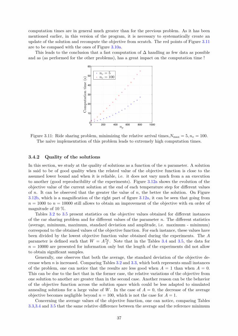
computation times are in general much greater than for the previous problem. As it has beenmentioned earlier, in this version of the program, it is necessary to systematically create anupdate of the solution and recompute the objective from scratch. The red points of Figure 3.11are to be compaed with the ones of Figure 3.10a.

This leads to the conclusion that a fast computation of � handling as few data as possibleand as (as performed for the other problems), has a great impact on the computation time !

0 200 400 600 800 10000

10

20

30

40

50

60

np

Com

putation

time(s)

nv = 5nv = 100

Figure 3.11: Ride sharing problem, minimizing the relative arrival times,Nmax

= 5, nv

= 100.The naïve implementation of this problem leads to extremely high computation times.

3.4.2 Quality of the solutionsIn this section, we study at the quality of solutions as a function of the n parameter. A solutionis said to be of good quality when the related value of the objective function is close to theassumed lower bound and when it is reliable, i.e. it does not vary much from a an executionto another (good reproducibility of the experiments). Figure 3.12a shows the evolution of theobjective value of the current solution at the end of each temperature step for di�erent valuesof n. It can be observed that the greater the value of n, the better the solution. On Figure3.12b, which is a magnification of the right part of figure 3.12a, it can be seen that going fromn = 1000 to n = 10000 still allows to obtain an improvement of the objective with en order ofmagnitude of 10 %.

Tables 3.2 to 3.5 present statistics on the objective values obtained for di�erent instancesof the car sharing problem and for di�erent values of the parameter n. The di�erent statistics(average, minimum, maximum, standard deviation and amplitude, i.e. maximum - minimum)correspond to the obtained values of the objective function. For each instance, these values havebeen divided by the lowest objective function value obtained during the experiments. The Aparameter is defined such that W = A

n

p

2

. Note that in the Tables 3.4 and 3.5, the data forn = 10000 are presented for information only but the length of the experiments did not allowto obtain significant samples.

Generally, one observes that both the average, the standard deviation of the objective de-crease when n is increased. Comparing Tables 3.2 and 3.3, which both represents small instancesof the problem, one can notice that the results are less good when A = 1 than when A = 0.This can be due to the fact that in the former case, the relative variations of the objective fromone solution to another are greater than in the second case. Another reason can be the behaviorof the objective function across the solution space which could be less adapted to simulatedannealing solutions for a large value of W . In the case of A = 0, the decrease of the averageobjective becomes negligible beyond n = 100, which is not the case for A = 1.

Concerning the average values of the objective function, one can notice, comparing Tables3.3,3.4 and 3.5 that the same relative di�erence between the average and the reference minimum

37

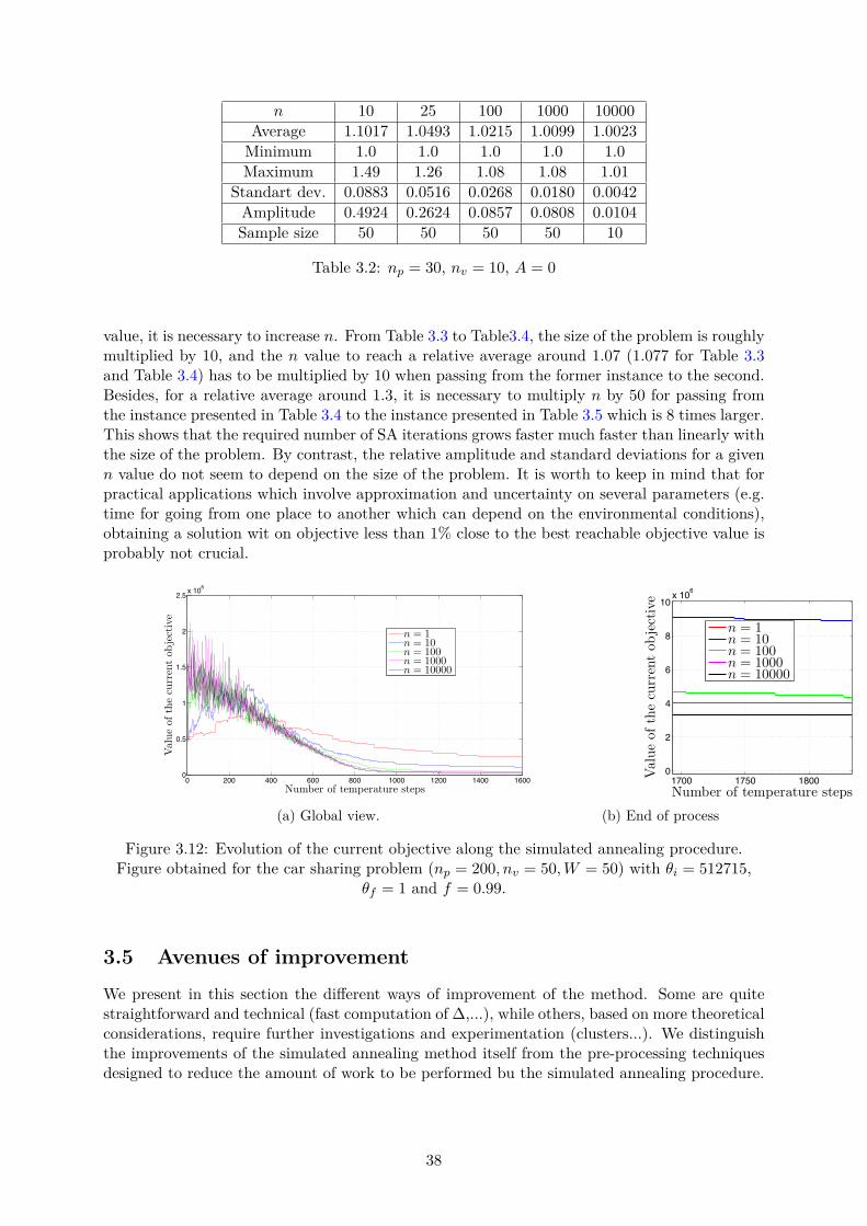
n 10 25 100 1000 10000Average 1.1017 1.0493 1.0215 1.0099 1.0023

Minimum 1.0 1.0 1.0 1.0 1.0Maximum 1.49 1.26 1.08 1.08 1.01

Standart dev. 0.0883 0.0516 0.0268 0.0180 0.0042Amplitude 0.4924 0.2624 0.0857 0.0808 0.0104Sample size 50 50 50 50 10

Table 3.2: np

= 30, nv

= 10, A = 0

value, it is necessary to increase n. From Table 3.3 to Table3.4, the size of the problem is roughlymultiplied by 10, and the n value to reach a relative average around 1.07 (1.077 for Table 3.3and Table 3.4) has to be multiplied by 10 when passing from the former instance to the second.Besides, for a relative average around 1.3, it is necessary to multiply n by 50 for passing fromthe instance presented in Table 3.4 to the instance presented in Table 3.5 which is 8 times larger.This shows that the required number of SA iterations grows faster much faster than linearly withthe size of the problem. By contrast, the relative amplitude and standard deviations for a givenn value do not seem to depend on the size of the problem. It is worth to keep in mind that forpractical applications which involve approximation and uncertainty on several parameters (e.g.time for going from one place to another which can depend on the environmental conditions),obtaining a solution wit on objective less than 1% close to the best reachable objective value isprobably not crucial.

0 200 400 600 800 1000 1200 1400 16000

0.5

1

1.5

2

2.5 x 108

Number of temperature steps

Valueofthecurrentobjective

n = 1n = 10n = 100n = 1000n = 10000

(a) Global view.

1700 1750 18000

2

4

6

8

10x 106

Number of temperature steps

Valueofthecu

rrentobjective

n = 1n = 10n = 100n = 1000n = 10000

(b) End of process

Figure 3.12: Evolution of the current objective along the simulated annealing procedure.Figure obtained for the car sharing problem (n

p

= 200, nv

= 50, W = 50) with ◊i

= 512715,◊

f

= 1 and f = 0.99.

3.5 Avenues of improvementWe present in this section the di�erent ways of improvement of the method. Some are quitestraightforward and technical (fast computation of �,...), while others, based on more theoreticalconsiderations, require further investigations and experimentation (clusters...). We distinguishthe improvements of the simulated annealing method itself from the pre-processing techniquesdesigned to reduce the amount of work to be performed bu the simulated annealing procedure.

38

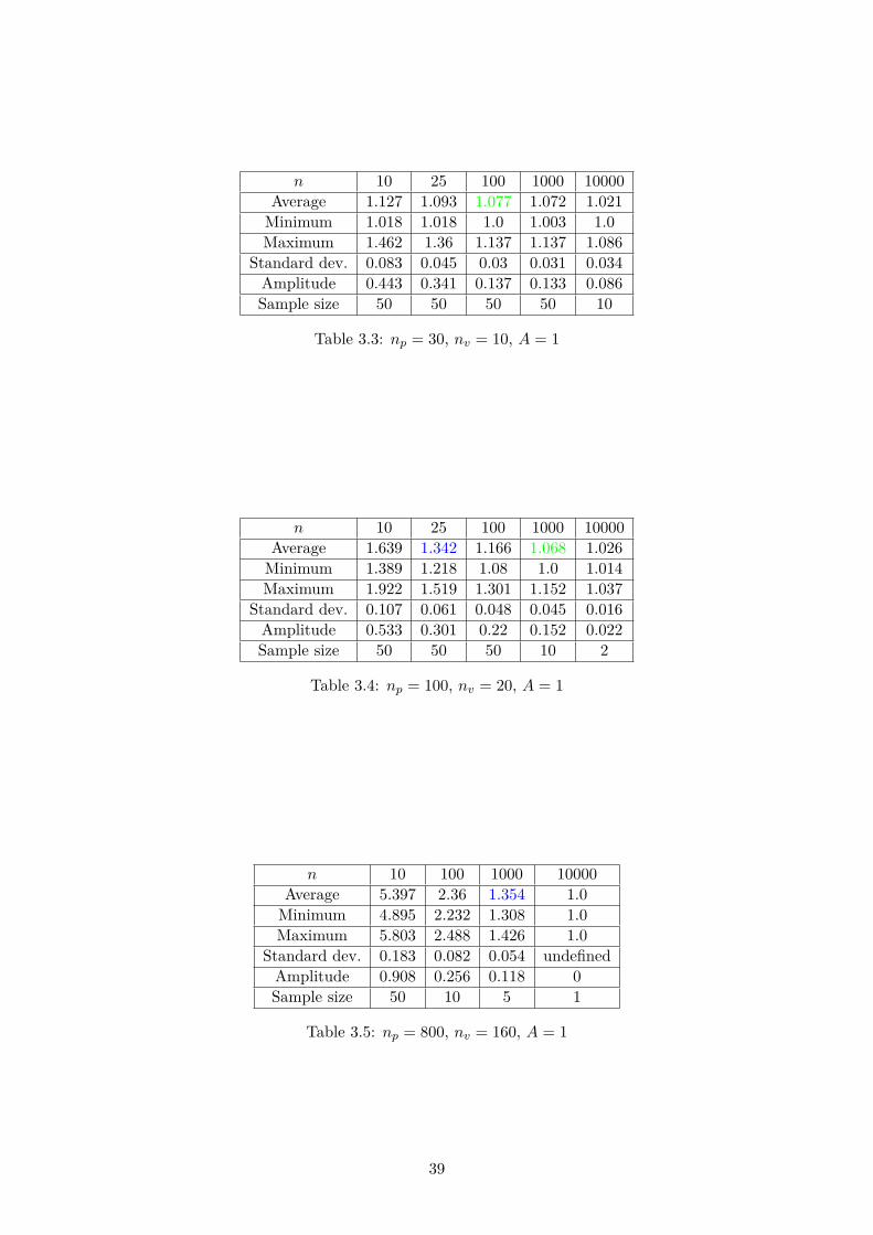
n 10 25 100 1000 10000Average 1.127 1.093 1.077 1.072 1.021

Minimum 1.018 1.018 1.0 1.003 1.0Maximum 1.462 1.36 1.137 1.137 1.086

Standard dev. 0.083 0.045 0.03 0.031 0.034Amplitude 0.443 0.341 0.137 0.133 0.086Sample size 50 50 50 50 10

Table 3.3: np

= 30, nv

= 10, A = 1

n 10 25 100 1000 10000Average 1.639 1.342 1.166 1.068 1.026

Minimum 1.389 1.218 1.08 1.0 1.014Maximum 1.922 1.519 1.301 1.152 1.037

Standard dev. 0.107 0.061 0.048 0.045 0.016Amplitude 0.533 0.301 0.22 0.152 0.022Sample size 50 50 50 10 2

Table 3.4: np

= 100, nv

= 20, A = 1

n 10 100 1000 10000Average 5.397 2.36 1.354 1.0

Minimum 4.895 2.232 1.308 1.0Maximum 5.803 2.488 1.426 1.0

Standard dev. 0.183 0.082 0.054 undefinedAmplitude 0.908 0.256 0.118 0Sample size 50 10 5 1

Table 3.5: np

= 800, nv

= 160, A = 1

39

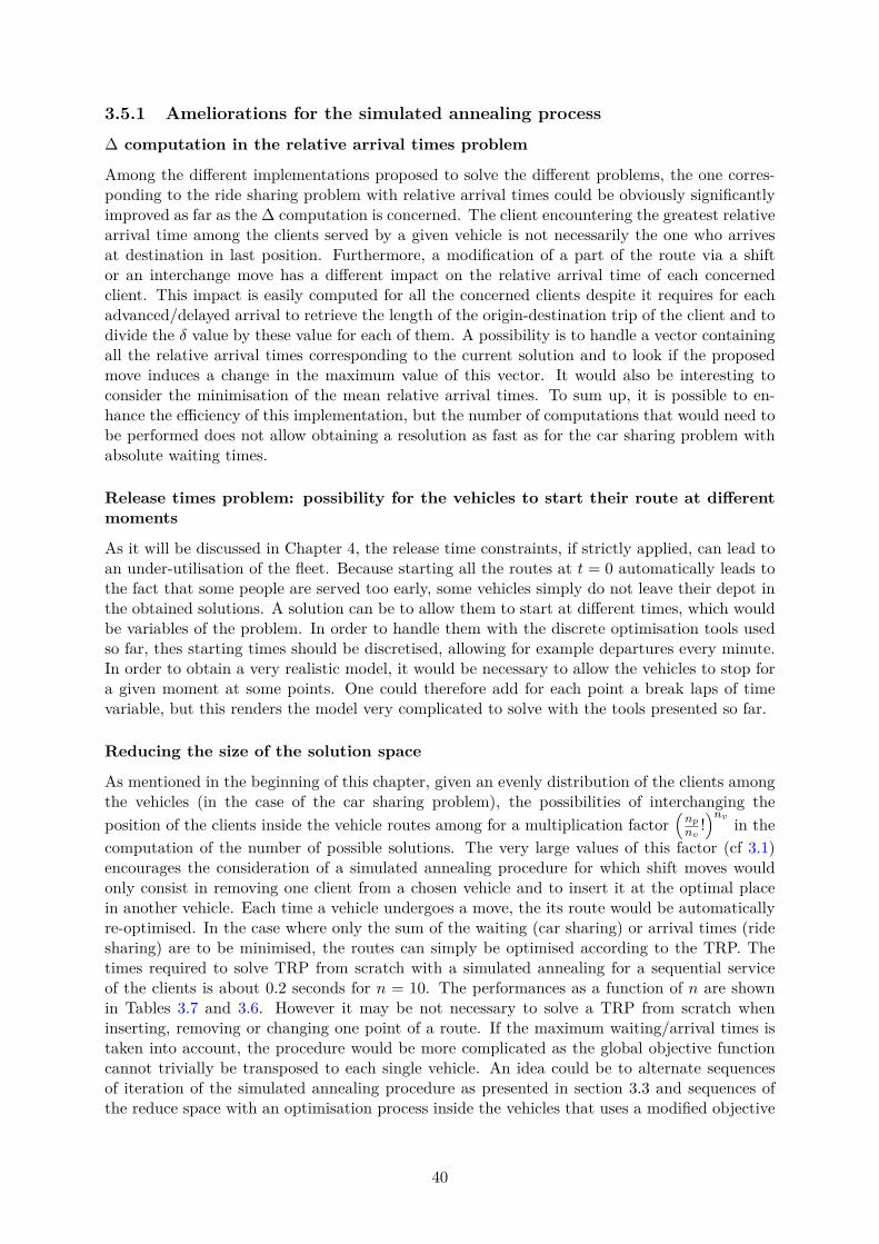
3.5.1 Ameliorations for the simulated annealing process� computation in the relative arrival times problem

Among the di�erent implementations proposed to solve the di�erent problems, the one corres-ponding to the ride sharing problem with relative arrival times could be obviously significantlyimproved as far as the � computation is concerned. The client encountering the greatest relativearrival time among the clients served by a given vehicle is not necessarily the one who arrivesat destination in last position. Furthermore, a modification of a part of the route via a shiftor an interchange move has a di�erent impact on the relative arrival time of each concernedclient. This impact is easily computed for all the concerned clients despite it requires for eachadvanced/delayed arrival to retrieve the length of the origin-destination trip of the client and todivide the ” value by these value for each of them. A possibility is to handle a vector containingall the relative arrival times corresponding to the current solution and to look if the proposedmove induces a change in the maximum value of this vector. It would also be interesting toconsider the minimisation of the mean relative arrival times. To sum up, it is possible to en-hance the e�ciency of this implementation, but the number of computations that would need tobe performed does not allow obtaining a resolution as fast as for the car sharing problem withabsolute waiting times.

Release times problem: possibility for the vehicles to start their route at di�erent

moments

As it will be discussed in Chapter 4, the release time constraints, if strictly applied, can lead toan under-utilisation of the fleet. Because starting all the routes at t = 0 automatically leads tothe fact that some people are served too early, some vehicles simply do not leave their depot inthe obtained solutions. A solution can be to allow them to start at di�erent times, which wouldbe variables of the problem. In order to handle them with the discrete optimisation tools usedso far, thes starting times should be discretised, allowing for example departures every minute.In order to obtain a very realistic model, it would be necessary to allow the vehicles to stop fora given moment at some points. One could therefore add for each point a break laps of timevariable, but this renders the model very complicated to solve with the tools presented so far.

Reducing the size of the solution space

As mentioned in the beginning of this chapter, given an evenly distribution of the clients amongthe vehicles (in the case of the car sharing problem), the possibilities of interchanging theposition of the clients inside the vehicle routes among for a multiplication factor

1n

p

n

v

!2

n

v in thecomputation of the number of possible solutions. The very large values of this factor (cf 3.1)encourages the consideration of a simulated annealing procedure for which shift moves wouldonly consist in removing one client from a chosen vehicle and to insert it at the optimal placein another vehicle. Each time a vehicle undergoes a move, the its route would be automaticallyre-optimised. In the case where only the sum of the waiting (car sharing) or arrival times (ridesharing) are to be minimised, the routes can simply be optimised according to the TRP. Thetimes required to solve TRP from scratch with a simulated annealing for a sequential serviceof the clients is about 0.2 seconds for n = 10. The performances as a function of n are shownin Tables 3.7 and 3.6. However it may be not necessary to solve a TRP from scratch wheninserting, removing or changing one point of a route. If the maximum waiting/arrival times istaken into account, the procedure would be more complicated as the global objective functioncannot trivially be transposed to each single vehicle. An idea could be to alternate sequencesof iteration of the simulated annealing procedure as presented in section 3.3 and sequences ofthe reduce space with an optimisation process inside the vehicles that uses a modified objective

40

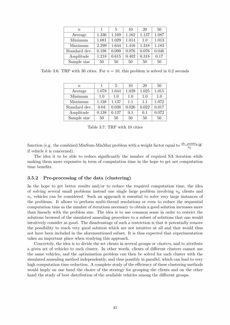
n 1 5 10 20 50Average 1.336 1.169 1.162 1.137 1.087

Minimum 1.081 1.029 1.014 1.0 1.013Maximum 2.299 1.644 1.416 1.318 1.183

Standard dev. 0.198 0.099 0.076 0.076 0.046Amplitude 1.218 0.615 0.402 0.318 0.17Sample size 50 50 50 50 50

Table 3.6: TRP with 30 cities. For n = 10, this problem is solved in 0.2 seconds

n 1 5 10 20 50Average 1.078 1.044 1.029 1.025 1.015

Minimum 1.0 1.0 1.0 1.0 1.0Maximum 1.138 1.137 1.1 1.1 1.072

Standard dev. 0.04 0.038 0.026 0.022 0.017Amplitude 0.138 0.137 0.1 0.1 0.072Sample size 50 50 50 50 50

Table 3.7: TRP with 10 cities

function (e.g. the combined MinSum-MinMax problem with a weight factor equal to nb_points

k

n

p

W

if vehicle k is concerned).The idea it to be able to reduce significantly the number of required SA iteration while

making them more expensive in term of computation time in the hope to get net computationtime benefits.

3.5.2 Pre-processing of the data (clustering)In the hope to get better results and/or to reduce the required computation time, the ideaof solving several small problems instead one single large problem involving n

p

clients andn

v

vehicles can be considered. Such an approach is essential to solve very large instances ofthe problems. It allows to perform multi-thread resolutions or even to reduce the sequentialcomputation time as the number of iterations necessary to obtain a good solution increases morethan linearly with the problem size. The idea is to use common sense in order to restrict thesolutions browsed of the simulated annealing procedure to a subset of solutions that one wouldintuitively consider as good. The disadvantage of such a restriction is that it potentially removethe possibility to reach very good solution which are not intuitive at all and that would thusnot have been included in the aforementioned subset. It is thus expected that experimentationtakes an important place when studying this approach.

Concretely, the idea is to divide the set clients in several groups or clusters, and to attributea given set of vehicles to each cluster. In other words, clients of di�erent clusters cannot usethe same vehicles, and the optimisation problem can then be solved for each cluster with thesimulated annealing method independently, and thus possibly in parallel, which can lead to veryhigh computation time reduction. A complete study of the e�ciency of these clustering methodswould imply on one hand the choice of the strategy for grouping the clients and on the otherhand the study of best distribution of the available vehicles among the di�erent groups.

41

Definition of the distance between clients

It is essential to define a distance between each possible pair of clients, the idea being that twoclients separated by a too large distance cannot travel together and should be put in di�erentclusters. This distance is not necessarily an Euclidian distance geographical points, but ratheran abstract distance that can be defined following di�erent strategies. Then, the clusters can bedetermined by solving the Facility Location Problem. If we choose to determine n

c

clusters, thisproblem amounts to choose n

c

centroïds among the set of clients (the centroïds correspond to thefacilities) and to attribute each client to one of the centroïds. The objective is to minimise thesum of the distance of each client to their corresponding centroïd, taking into account constaintsabout the minimum size of the clusters.

Similar trips strategy

The most basic idea to create clusters is to group together clients that need to perform a similartrip. In this vision, two clients are considered as close to each other if both their starting pointsand destination points are respectively close to each other. One can thus define the distancebetween clients i and j with the arithmetic mean:

Dij

= 12 (C

i

or

,j

or

+ Ci

dest

,j

dest

) . (3.20)

By defining this distance, it is expected that the proposed solutions will include routesconstituted of a series of pick up in an area and, after a trip with a full vehicle, a series of clientsdrops. An example of clustering realised with this strategy for an artificially generated set ofdata modelling a morning peak hour situation is shown in Figure 3.13.

−150 −100 −50 0 50 100 150−150

−100

−50

0

50

100

150

x(Km)

y(K

m)

Figure 3.13: Example of clustering for an artificially generated set of data modelling a morningpeak hour with 100 clients with the similar trip strategy. The number of cluster is 5 and they

are constrained to a minimum size of 5 clients. Each color represents a cluster. The starsrepresent origin points and the diamonds represent destination points.

Successive trips strategy

Taking into account the fact that it is also possible for the vehicles to take new clients afterdropping others, the situation where the starting points of some clients are situated near thedestination point of another one who will use the same vehicle is interesting. One can define thedistance between two clients as

Dij

= min31

2 (Ci

or

,j

or

+ Ci

dest

,j

dest

) , Ci

dest

,j

or

, Ci

or

,j

dest

4. (3.21)

42

Demand corridors

By contrast with the previous ones, this definition of distance is based on geometric character-istics. Recall that in the framework of this work, it has been decided to work only with distancesbetween points that could without loss of generality be replaced real displacement times in bytaking speed limitations and the road network geometry into account. The following approach,however, is expected to work only in the framework of simple Euclidian distances.

In order to put in evidence the possibility to pick up or drop a client along a journey, weconsider that two clients are also close to each other when the smallest distance between thestarting or destination point of one of these clients and the line segment describing the demandjourney of the other is small and both segments are oriented in a similar way (both clients travelin a similar direction). The idea is to group together clients in corridors. The encapsulation ofdemand into corridors is a concept that is also used for the design of classical pubic transportnetworks [14].

A graphical illustration of the three presented strategies is presented in Figure 3.14.

Figure 3.14: Illustration of the parameters taken into account in the di�erent method fordefining the distance between two client characterised by their origin-destination vectors (black

arrows). a) Similar journey strategy, b) Successive trips strategy, c) Corridors strategy. Thecolors represent the distances / angle taken into account.

Further investigations

The tests performed so far on a set of real data in the framework of a very general and hetero-geneous demand in a whole region did not lead neither to an amelioration of the results nor ato a decrease of the computation times. However, in dense population areas, it is not excludedthat the method would present good results. The aforementioned tests have been performedby distributing the vehicles evenly among the clusters but the link between the sum of the dis-tances between each clients of a cluster and the corresponding centroïd (or the average distancebetween the clients of a cluster) and the ideal size of the fleet to attribute to this cluster is stillto be investigated.

43

Chapter 4

Results analysis

The methods mentioned in Chapter 3 are now used to analyse qualitatively and quantitativelythe solutions proposed by the optimisation process that has been presented in Chapter 1. Thesolver is able to solve the following problem: we consider a fleet of public vehicles serving a setclients, and each client requires one vehicle to achieve a trip from their origin point to theirdestination point. The vehicles all start their tour at the same time, either from a given a pointreferred as a depot, or from the origin point of a client considered as optimal by the process. Inthe latter case, the starting point is said to be free. The vehicles do not have the possibility tostop until the end of their tour and they all ride at the same speed. In order to fix the ideas, theunique speed of 60 kilometres per hour will be considered. One can thus refer to a same vehicledisplacement by saying it is 10 km long or that it lasts 10 minutes. Finally, we distinguish carsharing problems from ride sharing problems. In the former case, a vehicle can transport onlyone client at once and it serves the di�erent clients sequentially while, in the second case, itis possible to carry several clients in a same vehicle provided the capacity of the vehicle is notexceeded. In the car sharing problem, the journey of a client is identical to the one they wouldhave followed with a personal car. On the other hand, they are likely to make detours in a ridesharing situation.

4.1 Solved problems definitions and notationsIn practice, four di�erent particular cases of the problem were implemented in the software:

1. The car sharing problem with simultaneous demand where a linear combination of the sum(and thus the average) of the waiting times and the maximum waiting time is minimised.

2. The ride sharing problem with simultaneous demand where a linear combination of the sum(and thus the average) of the waiting times and the maximum arrival time is minimised.

3. The ride sharing problem with simultaneous demand where a linear combination of thesum (and thus the average) of the arrival times and the maximum relative arrival time 1

is minimised.

4. The ride sharing problem with time-distributed demand. Only the average arrival time isminimised, which is equivalent to minimize the average laps of time between the desireddeparture time of a client and (referred as the release time) their arrival time.

The di�erent parameters that can be chosen for solving the problems for a given number np

of trip demands specified by an origin point, a destination point and for a wished starting time(only in Problem 4) are

1Recall that the relative arrival time of a client refers to their arrival time divided by the length of their trip.

44

• The number nv

of available vehicles;

• The capacity Nmax

of the vehicles (except for Problem 1);

• The value of the MinMax weight factor (W for Problems 1 and 2, Wrel

for Problem 3);

• The starting points (depots) of the vehicles. They can be either chosen randomly amongthe origin points of the clients, or left free, i.e. as a part of the problem to be solved.

The variables that can be observed to analyse a routing are for i œ {1, ..., np

} and j œ{1, ..., n

v

}

• The waiting time wi

of client i;

• The arrival time ai

of client i at their destination;

• The length of the journey li

of client i;

• The distance travelled by the vehicles Tk

;

• The number of clients served by a vehicle nb_clientsk

;

• The passenger load of each vehicle along time, i.e. the number of clients sitting this vehiclePop

k

(t);

• The time weighted average passenger load of the vehicles µ(Popk

) = 1

T

k

sT

k

0

Popk

(t)dt;

• The cumulated riding times of all the vehiclesq

n

v

k=1

Tk

, and the economy factor E =qn

v

k=1

T

kqn

p

i=1

trip

i

;

• The global average vehicle passenger load: M(Pop) =q

n

v

k=1

Tk

µ(Popk

);

• The advance ADVi

with which client i is served in Problem 4. A feasible solution corres-ponds to negative advances only. If ADV

i

Æ 0, wi

= ≠ADVi

.

Problem Name Simultataneity of the demand Objective functionProblem 1 Car sharing Yes

qi

wi

+ W maxi

wi

Problem 2 Ride sharing Yesq

i

ai

+ W maxi

ai

Problem 3 Ride sharing Yesq

i

ai

+ Wrel

maxi

a

i

trip

i

Problem 4 Ride sharing Noq

i

ai

+ Wadv

ADVi

Table 4.1: Summary of the problems solved by the current software. i always in the set ofclients.

A summary of the di�erent problems with their corresponding weighted sum-based objectivefunction is presented in Table 4.1. Recall that in Problem 4, the goal is to minimise

qi

ai

≠READY

i

where READYi

is the time by which client i wants to leave its origin point, which isequivalent to minimise

qi

ai

becauseq

i

READYi

is a constant. The term in Wadv

ADVi

in thetable allows to avoid cases where vehicles pick up clients too early.

The rest of this chapter will consist in the analyse of several aspects of the solutions proposedby the software for the di�erent problems. The set of data used (i.e.the set of origin-destinationpairs) will be in some cases a real and totally general demand covering a whole region containingseveral cities [10] and in some other cases artificially generated random data in order to put somephenomena in evidence. When talking about the real data set for a given number of clients n

p

,it means the first n

p

clients of the list.

45

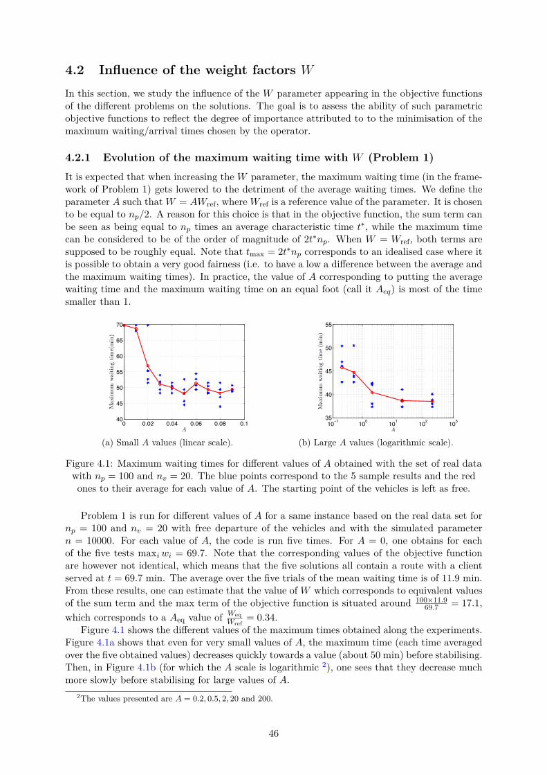
4.2 Influence of the weight factors W

In this section, we study the influence of the W parameter appearing in the objective functionsof the di�erent problems on the solutions. The goal is to assess the ability of such parametricobjective functions to reflect the degree of importance attributed to to the minimisation of themaximum waiting/arrival times chosen by the operator.

4.2.1 Evolution of the maximum waiting time with W (Problem 1)It is expected that when increasing the W parameter, the maximum waiting time (in the frame-work of Problem 1) gets lowered to the detriment of the average waiting times. We define theparameter A such that W = AW

ref

, where Wref

is a reference value of the parameter. It is chosento be equal to n

p

/2. A reason for this choice is that in the objective function, the sum term canbe seen as being equal to n

p

times an average characteristic time tú, while the maximum timecan be considered to be of the order of magnitude of 2tún

p

. When W = Wref

, both terms aresupposed to be roughly equal. Note that t

max

= 2túnp

corresponds to an idealised case where itis possible to obtain a very good fairness (i.e. to have a low a di�erence between the average andthe maximum waiting times). In practice, the value of A corresponding to putting the averagewaiting time and the maximum waiting time on an equal foot (call it A

eq

) is most of the timesmaller than 1.

0 0.02 0.04 0.06 0.08 0.140

45

50

55

60

65

70

A

Max

imum

waitingtime(min)

(a) Small A values (linear scale).

10−1 100 101 102 10335

40

45

50

55

A

Max

imum

waitingtime(m

in)

(b) Large A values (logarithmic scale).

Figure 4.1: Maximum waiting times for di�erent values of A obtained with the set of real datawith n

p

= 100 and nv

= 20. The blue points correspond to the 5 sample results and the redones to their average for each value of A. The starting point of the vehicles is left as free.

Problem 1 is run for di�erent values of A for a same instance based on the real data set forn

p

= 100 and nv

= 20 with free departure of the vehicles and with the simulated parametern = 10000. For each value of A, the code is run five times. For A = 0, one obtains for eachof the five tests max

i

wi

= 69.7. Note that the corresponding values of the objective functionare however not identical, which means that the five solutions all contain a route with a clientserved at t = 69.7 min. The average over the five trials of the mean waiting time is of 11.9 min.From these results, one can estimate that the value of W which corresponds to equivalent valuesof the sum term and the max term of the objective function is situated around 100◊11.9

69.7

= 17.1,which corresponds to a A

eq

value of W

eq

W

ref

= 0.34.Figure 4.1 shows the di�erent values of the maximum times obtained along the experiments.

Figure 4.1a shows that even for very small values of A, the maximum time (each time averagedover the five obtained values) decreases quickly towards a value (about 50 min) before stabilising.Then, in Figure 4.1b (for which the A scale is logarithmic 2), one sees that they decrease muchmore slowly before stabilising for large values of A.

2The values presented are A = 0.2, 0.5, 2, 20 and 200.

46

The strong decrease of the maximum times when going from A = 0 to A = 0.02 can beexplained by the fact that there exist solutions for which the maximum waiting is significantlyreduced with respect to the ones obtained with A = 0 without significantly increasing theaverage waiting time. A weak value of A is thus su�cient to make these solution appear. Thisphenomenon is to be put in relation with the large discrepancies in the set of trip demands(see Figure 4.2). According to Figure 4.1b, the largest decrease of the waiting times (apart forthe aforementioned one) happens for A values of orders of magnitude of 0.1 and 1, which isconsistent with the previous considerations.

0 20 40 60 80 100 1200

10

20

30

40

50

60

70

80

Trip (Km)

Number

ofconcerned

clients

Figure 4.2: Histogram of the length of the trip demands (origin-destination of the 100 clientsof the real data set).

So far, only values averaged over the di�erent experiments were discussed. However one cansee that for each mentioned value of A (except 0), there is a large deviation between the di�erentexperiments (amplitude up to 18 % in the data presented in Figure 4.1). This makes very di�cultto obtain a reliable control of the priority attributed to the minimisation of the maximum time.The reason are the inability of the used metaheuristic procedure to converge towards a uniquesolution and the fact that even for similar values of the objective function, it is possible tohave di�erent types of solution with di�erent repartition of the objective contribution of thetwo terms. This situation happens for moderate A values. In order to avoid this phenomenon,one could use the tools of multi-objective optimisation, for which there exist suitable simulatedannealing algorithms [22].

Knowing that there is always uncertainty about the priority e�ectively attributed to theminimisation of the maximum waiting time, one has to settle with empirical rules of goodpractices: ut A = 0 to totally neglect the maximum waiting times, take A ƒ A

eq

to attributethem a moderate priority and take A >> A

eq

to neglect the average waiting times.All these considerations can be extended to Problems 2 and 3 with adapted definitions of A.

For Problem 3, taking Wrel

= 1

2

qn

p

i=1

tripi

is enough to reach the saturation of the maximumrelative arrival time (around 4 against 24 for W

rel

= 0 with the same instance of the problem,for ride sharing with 5-place vehicles).

4.2.2 Penalty factor of Problem 4In our model of the ride sharing problem with release time (Problem 4), the vehicles do nothave the possibility to stop in order to wait for a client to be ready. If a large penalty coe�cientW

adv

is chosen, this leads the optimisation process to a solution where some available vehiclesdo not leave their depot in order to avoid serving any client in advance. In order to avoid thissituation, it is convenient to choose a reduced value of W

ADV

, which allows a reasonable advancefor a few clients when it is beneficial for the system. For the real data set with n

p

= 100 and

47

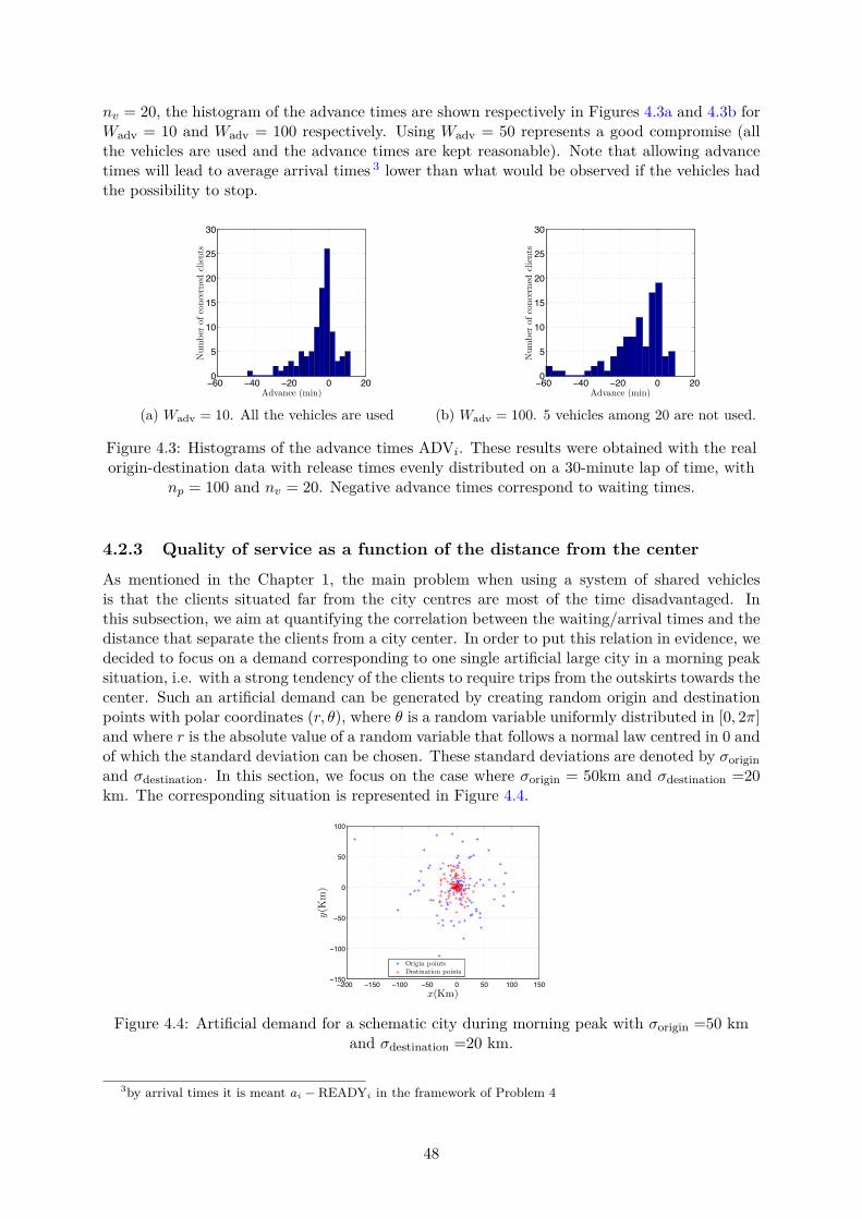
nv

= 20, the histogram of the advance times are shown respectively in Figures 4.3a and 4.3b forW

adv

= 10 and Wadv

= 100 respectively. Using Wadv

= 50 represents a good compromise (allthe vehicles are used and the advance times are kept reasonable). Note that allowing advancetimes will lead to average arrival times 3 lower than what would be observed if the vehicles hadthe possibility to stop.

−60 −40 −20 0 200

5

10

15

20

25

30

Advance (min)

Number

ofconcerned

clients

(a) Wadv = 10. All the vehicles are used

−60 −40 −20 0 200

5

10

15

20

25

30

Advance (min)

Number

ofconcerned

clients

(b) Wadv = 100. 5 vehicles among 20 are not used.

Figure 4.3: Histograms of the advance times ADVi

. These results were obtained with the realorigin-destination data with release times evenly distributed on a 30-minute lap of time, with

np

= 100 and nv

= 20. Negative advance times correspond to waiting times.

4.2.3 Quality of service as a function of the distance from the centerAs mentioned in the Chapter 1, the main problem when using a system of shared vehiclesis that the clients situated far from the city centres are most of the time disadvantaged. Inthis subsection, we aim at quantifying the correlation between the waiting/arrival times and thedistance that separate the clients from a city center. In order to put this relation in evidence, wedecided to focus on a demand corresponding to one single artificial large city in a morning peaksituation, i.e. with a strong tendency of the clients to require trips from the outskirts towards thecenter. Such an artificial demand can be generated by creating random origin and destinationpoints with polar coordinates (r, ◊), where ◊ is a random variable uniformly distributed in [0, 2fi]and where r is the absolute value of a random variable that follows a normal law centred in 0 andof which the standard deviation can be chosen. These standard deviations are denoted by ‡

origin

and ‡destination

. In this section, we focus on the case where ‡origin

= 50km and ‡destination

=20km. The corresponding situation is represented in Figure 4.4.

−200 −150 −100 −50 0 50 100 150−150

−100

−50

0

50

100

x(Km)

y(K

m)

Origin pointsDestination points

Figure 4.4: Artificial demand for a schematic city during morning peak with ‡origin

=50 kmand ‡

destination

=20 km.

3by arrival times it is meant ai

≠ READYi

in the framework of Problem 4

48

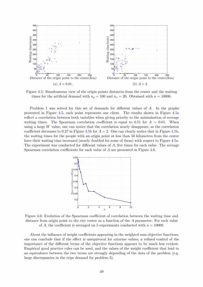
0 50 100 150 200 2500

50

100

150

200

250

300

350

400

450

500

Distance of the origin point to the center(Km)

Waitingtime(min)

(a) A = 0.01.

0 50 100 150 200 2500

50

100

150

200

250

300

350

400

450

500

Distance of the origin point to the center(Km)

Waitingtime(min)

(b) A = 2.

Figure 4.5: Simultaneous view of the origin points distances from the center and the waitingtimes for the artificial demand with n

p

= 100 and nv

= 20. Obtained with n = 10000.

Problem 1 was solved for this set of demands for di�erent values of A. In the graphspresented in Figure 4.5, each point represents one client. The results shown in Figure 4.5areflect a correlation between both variables when giving priority to the minimisation of averagewaiting times. The Spearman correlation coe�cient is equal to 0.51 for A = 0.01. Whenusing a large W value, one can notice that the correlation nearly disappears, as the correlationcoe�cient decreases to 0.27 in Figure 4.5b for A = 2. One can clearly notice that in Figure 4.5b,the waiting times for the people with an origin point at less than 50 kilometres from the centerhave their waiting time increased (nearly doubled for some of them) with respect to Figure 4.5a.The experiment was conducted for di�erent values of A, five times for each value. The averageSpearman correlation coe�cients for each value of A are presented in Figure 4.6.

0 2 4 6 8 10

0.2

0.25

0.3

0.35

0.4

0.45

0.5

0.55

A

Meancorrelationcoefficient

Figure 4.6: Evolution of the Spearman coe�cient of correlation between the waiting time anddistance from origin point to the city center as a function of the A parameter. For each value

of A, the coe�cient is averaged on 5 experiments conducted with n = 10000.

About the influence of weight coe�cients appearing in the weighted sum objective functions,one can conclude that if the e�ect is unequivocal for extreme values, a refined control of theimportance of the di�erent terms of the objective functions appears to be much less evident.Empirical good practice rules can be used, and the values of the weight coe�cient that lead toan equivalence between the two terms are strongly depending of the data of the problem (e.g.large discrepancies in the trips demand for problem 3).

49

4.3 Influence of the demand density on the quality of the ser-vice. Modelling with problems 2 and 4.

4.3.1 Influence of the density of the demandIn this section, we work on artificial data and build a demand corresponding to a city withthe same characteristic sizes as the one presented in the previous section (and represented inFigure 4.4): ‡

origin

= 50km and ‡destination

=20 km. It is thus once again a morning peaksituation. The idea is to generate three di�erent sets of demand with di�erent numbers of tripsrequirement (we take n

p

= 50, 100 and 200) while keeping the np

/na

ratio constant (nv

= 10, 20and 40 respectively). For all the experiments of this section, the starting point of the vehiclesis let as free. This instance was solved using three di�erent approaches: Problem 2 with withW = 0 and W = 100 and Problem 4 for w

adv

= 50. For this last problem, the release are timesrandomly generated and spread over 30 minutes. It is supposed that the capacity of the vehicleswas of 5 passengers. However, it has been noticed that when performing these experimentswith a very large value of N

max

, which makes the computations faster (see Chapter 3), thenumber of passengers hardly ever exceeds 4 5. The results are presented in Tables 4.2, 4.3 and4.4. Observing these three tables, one can see that the average waiting times and arrival timesare systematically decreased when the density of the demand increases. This reflects the factthat with a larger demand density, if the available resources are increased accordingly, thereare locally more possibilities of routing which allows to find better solution. The fact that themaximum arrival time does not decrease systematically when the density increases when solvingProblem 2 with W = 100 (Problem 2 being the only one among the three where maximumarrival time appears in the objective function) comes from the di�erences in the longest requiredtrips among the three instances. As matter of fact, when one looks at the maximum relativearrival times for this problem, one obtains 2.16 min, 2.41 min and 2.62 min for n

p

= 200,100and 50 respectively. Note that the mean length of the required trips for these three instances isrespectively of 42, 46 and 48 minutes.

4.3.2 Other considerationsBeside the study of the impacts of the density, it is visible that solving Problem 2 with W = 100is the approach that leads to the most economical routing. This can be understood intuitivelysince minimising the maximum arrival time means that the maximum length of the routes isalso minimised. Note that when solving Problem 4, the economy factor can get larger becauseof the detours that vehicles need to do in order to avoid taking people not ready to go. Tu putthis phenomenon in evidence the an instance of the problem was run with n

p

= 100 and nv

= 20but with release times spread over 80 minutes. The economy factor increases then to 0.94, i.e.this situation is nearly even bad as if each client used their own vehicle. Typical trajectories ofthe vehicles in such situations are presented in Figure 4.7a, to be compared with Figure 4.7b,which are trajectories obtained with Problem 2 (W = 100) and where the vehicles exhibit atendency to go from the outskirts to the center in a more straightforward way. Note that thevehicle represented by a red curve in Figure 4.7b is charged to perform an inner peripheral tour.

The temporal aspect of vehicles tours and the journeys of the corresponding clients can alsobe represented graphically via a set of time lines. In Figure 4.8, time lines for the 5 clients usingthe vehicle represented by a green curve in Figure 4.7a are represented. They allow to visualisethe laps of time the clients would have spend in their private vehicles if not using the publictransport system and time by which they begin and end their journey in the public vehicle.

4Among all these experiments, the largest fraction of the total riding timeq

nv

k=1

Tk

spent with a number ofpassengers larger than 5 is of 2.5 %. It is believed that imposing the capacity constraint would not change theresults in a significant way. The computations were thus performed with N

max

= 50.

50

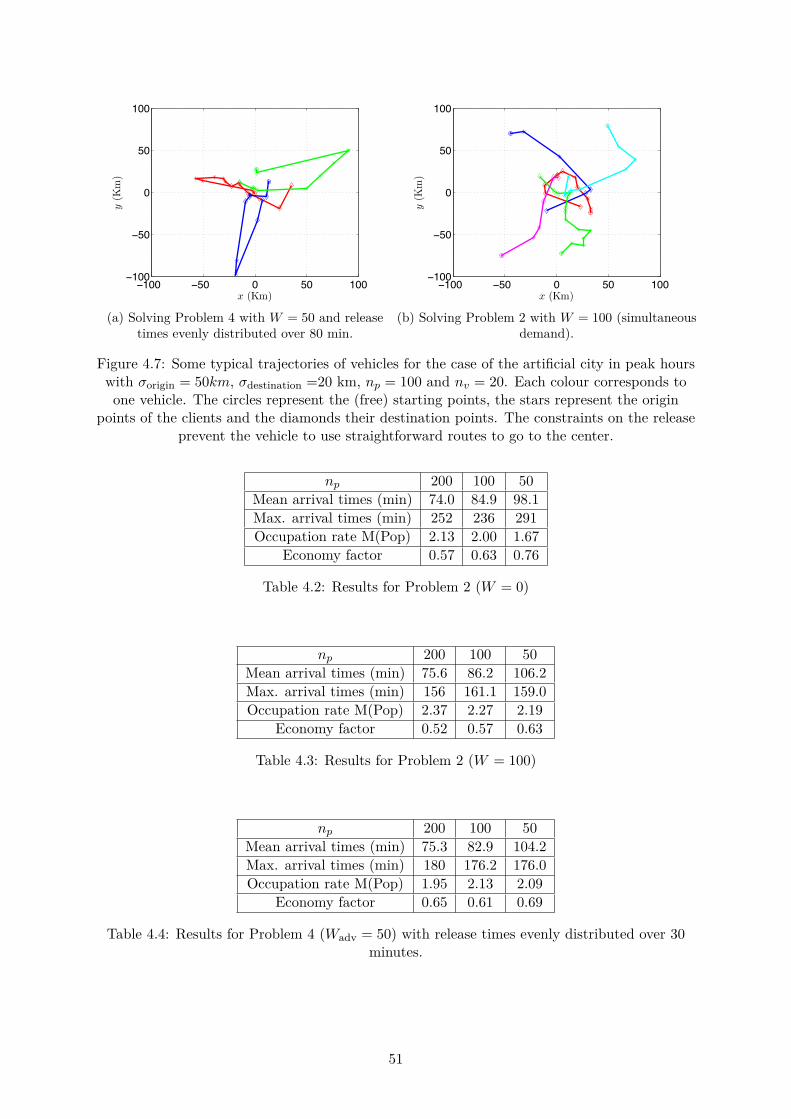
−100 −50 0 50 100−100

−50

0

50

100

x (Km)

y(K

m)

(a) Solving Problem 4 with W = 50 and releasetimes evenly distributed over 80 min.

−100 −50 0 50 100−100

−50

0

50

100

x (Km)

y(K

m)

(b) Solving Problem 2 with W = 100 (simultaneousdemand).

Figure 4.7: Some typical trajectories of vehicles for the case of the artificial city in peak hourswith ‡

origin

= 50km, ‡destination

=20 km, np

= 100 and nv

= 20. Each colour corresponds toone vehicle. The circles represent the (free) starting points, the stars represent the origin

points of the clients and the diamonds their destination points. The constraints on the releaseprevent the vehicle to use straightforward routes to go to the center.

np

200 100 50Mean arrival times (min) 74.0 84.9 98.1Max. arrival times (min) 252 236 291Occupation rate M(Pop) 2.13 2.00 1.67

Economy factor 0.57 0.63 0.76

Table 4.2: Results for Problem 2 (W = 0)

np

200 100 50Mean arrival times (min) 75.6 86.2 106.2Max. arrival times (min) 156 161.1 159.0Occupation rate M(Pop) 2.37 2.27 2.19

Economy factor 0.52 0.57 0.63

Table 4.3: Results for Problem 2 (W = 100)

np

200 100 50Mean arrival times (min) 75.3 82.9 104.2Max. arrival times (min) 180 176.2 176.0Occupation rate M(Pop) 1.95 2.13 2.09

Economy factor 0.65 0.61 0.69

Table 4.4: Results for Problem 4 (Wadv

= 50) with release times evenly distributed over 30minutes.

51

0 50 100 150 200 2500

1

2

3

4

5

6

Time (min)

Clientlabel

With a personal carUsing the system

Figure 4.8: Time lines for the clients served by the vehicle with trajectory represented in greenin Figure 4.7a. Client 1 is served slightly before their release time. Client 4 and 5 leave their

origin points by a time at which they would already be arrived at destination with theirprivate car.

4.4 Quality of the service as a function of the available fleetThe question of the practical application of the car sharing or ride sharing system was up tonow not addressed. In this section, we try to determine, in a given situation, the size of thefleet required in order to obtain reasonable waiting and arrival times. The usefulness of such asystem in areas that are subject to tra�c congestion is also discussed.

The problem is run on an artificial set of demands representing a city similar the one usedso far, but with smaller characteristic dimensions (‡

origin

= 25km and ‡destination

=10 km) forn

p

= 100, and several sizes of fleet are tried. The obtained results are shown in Tables 4.5,4.6 and 4.7. The departure position of the vehicles is free. All the situations are approachedwith the same three problems as in the previous section (Problem 2 with W = 0 and 100 andProblem 4 with W

adv

= 50.) The average length of the required trips is 20 km. The experimentsare performed with infinite capacities, but the results in the hypothesis of 5-places vehicles arevalid for all the experiments (the number of passenger in the vehicles do not exceed 5 for morethan 3 % of the times), except for n

v

= 10, where the number of passengers exceeds 5 duringup to 14 % of the time depending from the approach used.

nv

30.0 25.0 20.0 15.0 10.0Mean waiting times times (min) 6.72 9.61 12.9 18.5 29.47

Max. waiting times (min) 27.42 37.9 71.8 79.1 118.45Mean arrival times (min) 29.5 33.1 37.1 45.04 58.5Max. arrival times (min) 65.9 75.2 116.5 127.1 161.04Occupation rate M(Pop) 1.81 1.91 1.9 2.2 2.25

Economy factor E 0.62 0.61 0.63 0.6 0.64

Table 4.5: Impact of the size of the fleet on the service for a morning peak hour configurationfor a randomly generated demand corresponding to a city with dimensions ‡

origin

= 25km and‡

destination

=10 km. Results for Problem 2 (W = 0)

52

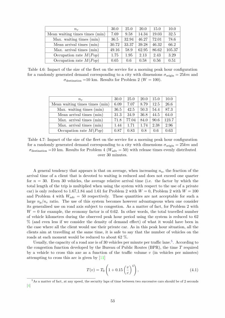
nv

30.0 25.0 20.0 15.0 10.0Mean waiting times times (min) 7.69 9.58 14.34 19.03 32.5

Max. waiting times (min) 36.5 32.94 46.27 72.01 78.6Mean arrival times (min) 30.72 33.37 39.28 46.32 66.2Max. arrival times (min) 49.16 58.9 62.95 86.62 105.37Occupation rate M(Pop) 1.75 1.95 2.13 2.43 3.29Occupation rate M(Pop) 0.65 0.6 0.58 0.56 0.51

Table 4.6: Impact of the size of the fleet on the service for a morning peak hour configurationfor a randomly generated demand corresponding to a city with dimensions ‡

origin

= 25km and‡

destination

=10 km. Results for Problem 2 (W = 100).

nv

30.0 25.0 20.0 15.0 10.0Mean waiting times times (min) 6.09 7.07 8.79 12.5 26.6

Max. waiting times (min) 36.5 42.5 50.3 54.4 87.3Mean arrival times (min) 31.3 34.9 36.8 44.5 64.0Max. arrival times (min) 71.8 77.04 84.0 90.6 123.7Max. arrival times (min) 1.44 1.71 1.74 2.38 2.96Occupation rate M(Pop) 0.87 0.83 0.8 0.6 0.63

Table 4.7: Impact of the size of the fleet on the service for a morning peak hour configurationfor a randomly generated demand corresponding to a city with dimensions ‡

origin

= 25km and‡

destination

=10 km. Results for Problem 4 (Wadv

= 50) with release times evenly distributedover 30 minutes.

A general tendency that appears is that on average, when increasing na

, the fraction of thearrival time of a client that is devoted to waiting is reduced and does not exceed one quarterfor n = 30. Even 30 vehicles, the average relative arrival time (i.e. the factor by which thetotal length of the trip is multiplied when using the system with respect to the use of a privatecar) is only reduced to 1.67,1.84 and 1.61 for Problem 2 with W = 0, Problem 2 with W = 100and Problem 4 with W

adv

= 50 respectively. These quantities are not acceptable for such alarge n

p

/nv

ratio. The use of this system becomes however advantageous when one considerits generalised use on road axis subject to congestion. As a matter of fact, for Problem 2 withW = 0 for example, the economy factor is of 0.62. In other words, the total travelled numberof vehicle kilometres during the observed peak hour period using the system is reduced to 62% (and even less if we consider the density of demand e�ect) of what it would have been inthe case where all the client would use their private car. As in this peak hour situation, all theclients aim at travelling at the same time, it is safe to say that the number of vehicles on theroads at each moment would be reduced to about 62 %.

Usually, the capacity of a road axe is of 30 vehicles per minute per tra�c lane.5. According tothe congestion function developed by the Bureau of Public Routes (BPR), the time T requiredby a vehicle to cross this axe as a function of the tra�c volume v (in vehicles per minutes)attempting to cross this arc is given by [11]

T (v) = T0

A

1 + 0.153

v

c

44

B

, (4.1)

5As a matter of fact, at any speed, the security laps of time between two successive cars should be of 2 seconds[4]

53

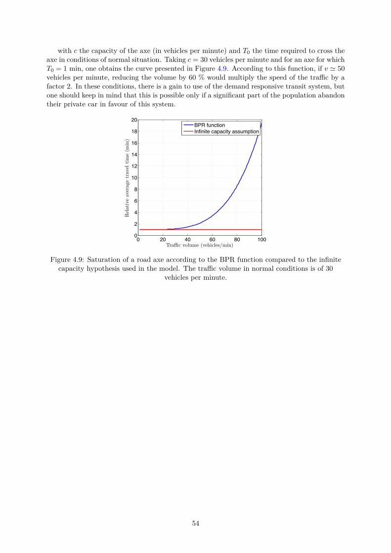
with c the capacity of the axe (in vehicles per minute) and T0

the time required to cross theaxe in conditions of normal situation. Taking c = 30 vehicles per minute and for an axe for whichT

0

= 1 min, one obtains the curve presented in Figure 4.9. According to this function, if v ƒ 50vehicles per minute, reducing the volume by 60 % would multiply the speed of the tra�c by afactor 2. In these conditions, there is a gain to use of the demand responsive transit system, butone should keep in mind that this is possible only if a significant part of the population abandontheir private car in favour of this system.

0 20 40 60 80 1000

2

4

6

8

10

12

14

16

18

20

Traffic volume (vehicles/min)

Relativeaverag

etravel

time(m

in)

BPR functionInfinite capacity assumption

Figure 4.9: Saturation of a road axe according to the BPR function compared to the infinitecapacity hypothesis used in the model. The tra�c volume in normal conditions is of 30

vehicles per minute.

54

Chapter 5

Conclusions and perspectives

The objective of this work was to develop an optimisation process in order to determine theroutes of a fleet of public vehicles responding to a set of a priori specified demands for individualtrips. These public vehicles are supposed to be not driven by the client (common taxis or self-driving cars able to travel without passengers). Both the cases of car sharing (vehicles able totransport one client) and ride sharing (vehicles transporting several clients at the same time)were envisaged. The optimisation was based on the minimisation of the waiting times of theclients with the concern to obtain a routing of the vehicles both fast and fair. Variants of theproblem with a minimisation of the maximum factor by which a client multiplies the length oftheir personal-vehicle-based trip when using the system and with accounting of various releasetimes were also envisaged.

We showed that these problems can be modelled as Vehicle Routing Problems for which theobjective function, which classically represents sum of the costs for the operator, is replaced bya linear combination of the sum of the waiting / arrival times and their maximum.

Solving these problems even for small instances requires the use of heuristic or metaheur-istic methods. The simulated annealing metaheuristics was used in the framework of a localsearch procedure for a small neighbourhood. The method appears to give solutions for whichthe objective function converges towards a given value when the number of simulated annealingiterations increases and to solve better the problems in the limit case where only the aver-age waiting/arrival time is to be minimised. A precise control of the priority accorded to theminimisation of the maximum waiting / arrival time (very high or absent priority).

Applying the optimisation process to sets of trips demand, it was possible to put in evidencethe fact that when according a high priority to the maximum waiting time, the discrepanciesbetween the quality of the service delivered for the clients from the outskirts of a city with respectto the ones of the center can be reduced. The e�ciency of the system also appears to increasewith density of population for a fixed number of clients/number of vehicles ratio. Finally, inorder to be beneficial for the clients, the system should be used massively on road axis subject tocongestion in order lower the tra�c volume and to increase the commercial speed. This wouldcompensate the time spent waiting for a vehicle and devoted to detours. This naturally impliesthe use of vehicles capable of transporting several clients at the same time, car sharing beingonly useful to decrease the number of vehicles but would logically increase the tra�c volume.

This introductory work on the optimisation of a demand-responsive transit system pavesthe way for further research. On a modelling point of view, it is interesting to explore thepossibilities o�ered by multi-objective optimisation to obtain a better control of the impact ofthe priority attributed to the minimisation of maximum times.

On the methodological point of view, beyond the ways for improvement of the methodsugested in Chapter 3, some more sophisticated method could be envisaged. Laporte [12], forexample, developed a powerful simulated annealing-based method for solving the CCVRP (VRPminimising the sum of the visit times) which could potentially be extended to the problems solved

55

in this work. This method is based on en extension of the large neighbourhood search developedby Shawn in [21] and the simulated annealing procedure is enhanced with a system of scoringfor the moves.

A real time application of the optimisation process could be envisaged. It means that de-mands appearing during the service could be treated. One could for example solve the problemin a way similar to the one proposed in Chapter 3 but allowing only for small changes in theroutes in order to satisfy the new demands. As a matter of fact, some clients would already besitting inside the vehicles and the client that would have been waiting for a longer time shouldnot be disadvantaged. The addition of such constraints implies that the solution space could beconsiderably reduced with respect to the problem studied in this work, making fast real timecomputation possible.

56

Bibliography

[1] International Transport Forum., 2015. Urban Mobility System Upgrade: How Shared Self-Driving Cars Could Change City Tra�c. ITF.

[2] Gurobi Optimization website : http://www.gurobi.com.

[3] The julia language : https://julialang.org/.

[4] "Trop vite... Trop tard", Booklet of Institut Belge pour la Sérecurité Routière (IBSR).

[5] Applications of optimization with Xpress-MP. Dash Optimization Ltd., 2000.

[6] Rigole P.J. Andreasson I. Burghout, W. Impacts of shared autonomous taxis in a metro-politan area. Transportation Research Board 94th Annual Meeting, 2015.

[7] Scarborough B.A. Burns, L.D. Transforming personal mobility. Technical report, The EarthInstitute of Columbia University, 2013.

[8] Hermann W. Campbell AM, Vandenbussche D. Routingforreliefe�orts. TransportationScience, 2008.

[9] M. Cools. Toegepaste optimalisatietechnieken, 2003. Lecture notes.

[10] Eric Cornelis, Michel Hubert, Philippe Huynen, Kevin Lebrun, Geo�roy Patriarche, AstridDe Witte, Lieve Creemers, Katrien Declercq, Davy Janssens, Marie Castaigne, and et al.Belgian Daily Mobility (BELDAM): Enquête sur la mobilité quotidienne des belges. 2012.

[11] Ren Moses Enock T. Mtoi. Calibration and evaluation of link congestion functions: Apply-ing intrinsic sensitivity of link speed as a practical consideration to heterogeneous facilitytypes within urban network. Journal of Transportation Technologies, 4:141–149, 2014.

[12] GilbertLaporte Glaydston MattosRibeiro. An adaptive large neighborhood search heur-istic for the cumulative capacitated vehicle routing problem. Computers and OperationsResearch, 2012.

[13] Michal Maciejewskia Joschka Bischo�a. Autonomous taxicabs in berlin – a spatiotemporalanalysis of service performance. Transportation Research Procedia, 2016.

[14] C. Morency C. Berdier K. Bahbouh, J. R.Wagner. Travel demand corridors: Modellingapproach and relevance in the planning process. Journal of Transport Geography, 2017.

[15] Gilbert Laporte. The Vehicle Routing Problem: An overview of exact and approximatealgorithms. European Journal of Operational Research, 1992.

[16] J-Y Potvin M. Gendreau. Handbook of Metaheurisitcs, Second edition.

[17] Sabine Limbourg Mario Cools, Caroline Rongy. Can autonomous vehicles reduce car mo-bility ? Evidences from a stated adaptation experiment in Belgium. 2016.

57

[18] Sandra Ulrich NGUEVEU. Problèmes de tournées de véhicules avec contraintes particulièrespour la maîtrise des risques. PhD thesis, Université de Technologie de Troyes, 2009.

[19] W≥odzimierz Ogryczak and Tomasz Sliwinski. On equitable approaches to resource al-location problems: the conditional minimax solutions. Journal of telecommunication andinformation technology, 2002.

[20] I. H. Osman. Metastrategy simulated anealing and tabu search algorithms for the vehiclerouting problem. Annals of Operation Research, 1993.

[21] Shawn P. A new local search algorithm providing high quality solutions to vehicle routingproblems. Technical report, University of Strathclyde, Glasgow, 1997.

[22] B. Suman and P. Kumar. A survey of simulated annealing as a tool for single and multiob-jective optimization. Journal of Transportation Technologies, 2014.

[23] Mark S. Daskin Susan Hesse Owen. Strategic facility location: A review. European Journalof Operational Research, 1998.

[24] Nouraniy Y. and Andresenz B. A comparison of simulated annealing cooling strategies. J.Phys. A: Math. Gen, (31):8373–8385, 1998.

58