Division of Applied Mathematics

Master Thesis in Mathematics / Applied Mathematics

Valuation of cancelable interest rate swaps viaHull-White trinomial tree model

by

Sergii Gryshkevych

Masterarbete i matematik / tillampad matematik

Division of Applied MathematicsSchool of Education, Culture and Communication

Malardalen UniversitySE-721 23 Vasteras, Sweden

Division of Applied Mathematics

Master thesis in mathematics / applied mathematics

Date:

201X-MM-DD

Project name:

Valuation of cancelable interest rate swaps via Hull-White trinomial treemodel

Author :

Sergii Gryshkevych

Supervisor :

Prof. Jan M. Roman

Examiner :

Ass. Prof. Anatoliy Malyarenko

Comprising :

30 ECTS credits

Abstract

The thesis studies a problem of cancelable interest rate swap pricing viaHull-White trinomial tree model. Obtained valuation results are comparedto Swedbank internal valuation and are found to be consistent. Peculiaritiesof cancelable interest rate swap contracts, their replication and valuation viaHull-White trinomial tree model are investigated during the study. Obtainedmathematical results are implemented in Object Pascal.

Acknowledgements

I would like to thank my supervisor Prof. Jan M. Roman for his assistanceduring the research and provision of input data for the study. Also I amgrateful to Ass. Prof. Anatoliy Malyarenko for his valuable advices andsupport during my Master studies in Vasteras. Furthermore, I acknowledgeInvest Systems Sverige AB for granting the access to Delphi IDE and espe-cially Dr. Robin Lundgren and Mr. Johan Andersson for their assistancewith programming part of the thesis. And last but not the least. I say spe-cial thanks to Swedish Institute for providing me with funding and makingpossible my studies at Malardalen University.

Contents

1 Introduction 2

2 Short Note on Interest Rate Swaps and Swaptions 42.1 Main concepts . . . . . . . . . . . . . . . . . . . . . . . . . . . 42.2 Cancelable swaps . . . . . . . . . . . . . . . . . . . . . . . . . 62.3 Swap and swaption market . . . . . . . . . . . . . . . . . . . . 7

3 Theoretical framework 93.1 Black model . . . . . . . . . . . . . . . . . . . . . . . . . . . . 93.2 Hull-White trinomial tree model . . . . . . . . . . . . . . . . . 11

3.2.1 Interest rate equation . . . . . . . . . . . . . . . . . . . 123.2.2 Converting to tree process . . . . . . . . . . . . . . . . 133.2.3 Tree consistency with market term structure . . . . . . 153.2.4 Calibration . . . . . . . . . . . . . . . . . . . . . . . . 16

3.3 Constructing a yield curve . . . . . . . . . . . . . . . . . . . . 17

4 Model implementation 194.1 Overview of the developed application . . . . . . . . . . . . . 194.2 Valuation . . . . . . . . . . . . . . . . . . . . . . . . . . . . . 20

4.2.1 Constructing the tree . . . . . . . . . . . . . . . . . . . 214.2.2 Calibration . . . . . . . . . . . . . . . . . . . . . . . . 224.2.3 Results . . . . . . . . . . . . . . . . . . . . . . . . . . . 254.2.4 Cancellation premium . . . . . . . . . . . . . . . . . . 28

5 Conclusions 30

1

Chapter 1

Introduction

The primary goal of this thesis is to valuate a cancelable interest rate swapcontract, which is included into one of Swedbank’s portfolios. Results arecompared to internal bank valuation. This implies the following subproblems:

• Construct a model;

• Calibrate the model;

• Develop an application.

Hull-White trinomial tree model was selected for valuation purposes.Levenberg-Marquardt algorithm was used for optimization problem. Th ap-plication is developed in Object Pascal using Embracadero Delphi XE asintegrated development environment. Valuation of cancelable interest rateswap contracts is a non-trivial problem of financial engineering. Roughlyspeaking, the problem of cancelable interest rate swap valuation reduces toBermudan style option pricing. Due to complexity of the stated problemonly limited number of models are capable of pricing such type of contracts.The problem of cancelable interest rate swaps valuation is not very popularin the world of academia. We do not know many works on particularly can-celable iterest rate swaps subject. It is explained by the fact that cancelableswaps valuation is a derivative problem to a more general one — interest ratemodeling and bermudan options.

Patrick Hagan presents in [1] methodology of pricing cancelable interestrate swaps via Linear Gaussian Model (LGM). Brigo and Mercurio in [2]discuss general concepts of interest rate modelling. Hull and White in [3]investigate a question of interest rate derivative securities pricing. In [4]and [5] Hull and White introduce a procedure for constructing trinomialtrees for interest rate modeling and in [6] discuss model calibration issues.

2

The remainder of the thesis is organized as follows. Chapter 2 presentsmain concepts of interest rate swap and swaption contracts, peculiarities ofcancelable swap contracts and current state of interest rate derivatives con-tracts market. Chapter 3 contains description of Black 76 model and explicitpresentation of Hull-White trinomial tree model where we show step-by-stepanalytical derivation of lattice representation. In addition, yield curve con-struction method is also presented in Chapter 3. Chapter 4 discusses obtainedresults of model implementation while Chapter 5 sums up all achieved resultsand makes conclusions with suggestions for further research.

3

Chapter 2

Short Note on Interest RateSwaps and Swaptions

This chapter deals with interest rate swaps and swaptions contract’s concepts,discusses in details idea of cancelable swap cotract.

2.1 Main concepts

The following two definitions are taken from [7].

Definition (Swap). “An agreement to exchange cash flows in the future ac-cording to a prearranged formula.”

Generally speaking, cash flows can be defined in a wide variety of ways. Acash flow can be linked to an interest rate, currency price, commodity priceor even to a trigger on some event — default of the obligation, for example.The most widespread type of swap contract is a, so called, plain vanilla swap.With this type of contract one side cash flows are based on a fixed rate ona notional principal amount, while, on the other side, cash flows are linkedto some index1 which evolves as the time flows. If a company agrees to paycash flows based on a fixed rate in exchange for floating payments this is apayer swap. On the contrary, receiver swap implies paying at a floating rateand receiving fixed interest.

Definition (Swap option). “An option to enter into an interest rate swapwhere a specified fixed rate is exchanged for floating.”

1It can be LIBOR, STIBOR, EURIBOR, etc.

4

Swap options, or swaptions, give the holder the right, but not the obli-gation, to enter into a certain interest rate swap at a certain time in thefuture.

From now we will refer to swap instead of interest rate swap and toswaption instead of swap option.

Usually, following types of swaptions are distinguished.

1 Depending on execution type:

• European — executable on a specific date;

• American — executable at any time during the lifetime of thecontract;

• Bermuda — executable during specific period of time.

2 Depending on underlying swap type:

• Payer — gives right to enter payer swap contract;

• Receiver — gives right to enter receiver swap contract.

We will examine in more details last two types of swaptions, as, sometimes,it might be tricky to understand, which type of contract is actually behindthe definition.

Common practice is is to understand a call swaption as an option ona payer swap, thus the buyer of the call swaption buys the right to enterinto a interest rate swap as fixed rate payer. However, if one enters a query“call swaption definition” in Google, directly contrasting results can be foundamong first ten ones.

For example, website www.investorwords.com gives the following commondefinition:

“A swaption in which the buyer has the right to enter into a swapas a fixed-rate payer.”

At the same time website www.invest.yourdictionary.com gives the oppositedefinition:

“A swaption is an option to enter into an interest rate swap at aspecified future date with the call giving the purchaser the right,but not the obligation, to receive a fixed interest rate.”

The problem is that they are both correct. The source of discrepancy liesin the convention, which right underlies the option — to pay fixed rate orto receive it. If option is written on the right to make fixed rate payments,

5

then call means payer. But if option is written on the right to receive fixedrate payments call means receiver.

To summarize stated above, the following table will enable the reader todetermine type of the contract correctly.

Fixed FloatingCall Payer ReceiverPut Receiver Payer

Table 2.1: Types of swaption contracts

2.2 Cancelable swaps

The following definition cites [8].

Definition (Cancelable swap). “A plain vanilla swap where the one of thecounterparties has the right but not the obligation to terminate the swap onone or more predetermined dates during the life of the swap.”

Cancelable swaps can be divided into callable and puttable. In a callableswap the party which pays fixed rate has the right to terminate the contract.In a puttable one the fixed rate receiving party has a possibility to terminatethe contract. In both cases termination dates are specified by the contractand, in most cases, are the same as reset dates.

For purposes of valuation cancelable swap is replicated by plain vanillainterest rate swap (swap body) and option on an opposite swap (cancella-tion premium). Indeed, a callable swap is a combination of plain-vanillaswap and a receiver swaption, while a puttable swap is a plain-vanilla one incombination with a payer swaption. While plain vanilla interest rate swapis a well-known interest rate instrument, cancellation premium needs moredetailed discussion.

Cancellation premium is determined as follows. Canceling a swap con-tract is equal to entering an opposite one with the same parameters. For ex-ample, receiver interest rate swap can be cancelled by setting up a payer one,providing all other parameters like notional amounts, maturity, fixed rate andfloating leg index are the same. So, we see cancellation of the payer/receiverswap with fixed rate x% as a Bermuda style variable American option ona receiver/payer swap with strike x%. But what does “variable” mean? Itmeans that the length of the underlying swap is dependent on time at whichthe option is exercised. To illustrate it let us consider an example.

6

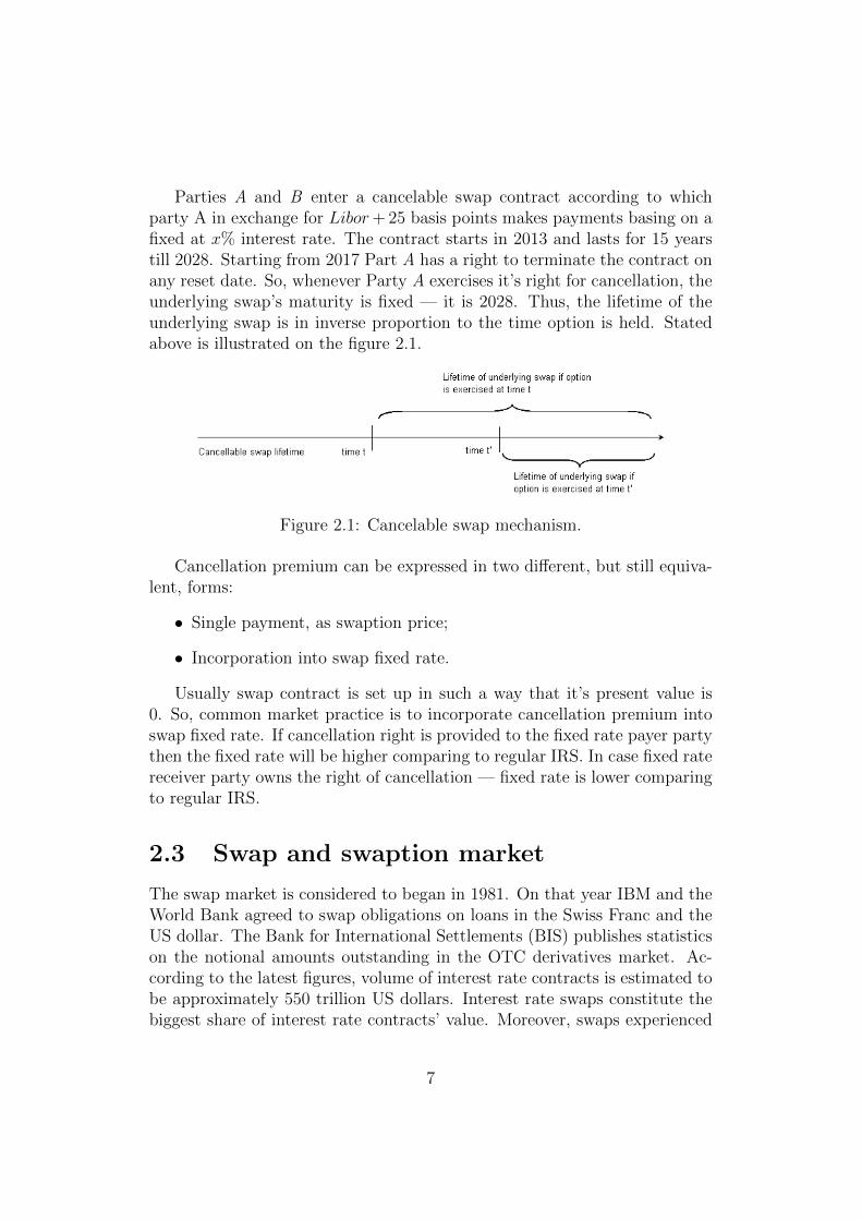
Parties A and B enter a cancelable swap contract according to whichparty A in exchange for Libor+ 25 basis points makes payments basing on afixed at x% interest rate. The contract starts in 2013 and lasts for 15 yearstill 2028. Starting from 2017 Part A has a right to terminate the contract onany reset date. So, whenever Party A exercises it’s right for cancellation, theunderlying swap’s maturity is fixed — it is 2028. Thus, the lifetime of theunderlying swap is in inverse proportion to the time option is held. Statedabove is illustrated on the figure 2.1.

Figure 2.1: Cancelable swap mechanism.

Cancellation premium can be expressed in two different, but still equiva-lent, forms:

• Single payment, as swaption price;

• Incorporation into swap fixed rate.

Usually swap contract is set up in such a way that it’s present value is0. So, common market practice is to incorporate cancellation premium intoswap fixed rate. If cancellation right is provided to the fixed rate payer partythen the fixed rate will be higher comparing to regular IRS. In case fixed ratereceiver party owns the right of cancellation — fixed rate is lower comparingto regular IRS.

2.3 Swap and swaption market

The swap market is considered to began in 1981. On that year IBM and theWorld Bank agreed to swap obligations on loans in the Swiss Franc and theUS dollar. The Bank for International Settlements (BIS) publishes statisticson the notional amounts outstanding in the OTC derivatives market. Ac-cording to the latest figures, volume of interest rate contracts is estimated tobe approximately 550 trillion US dollars. Interest rate swaps constitute thebiggest share of interest rate contracts’ value. Moreover, swaps experienced

7

21% growth in volume during first half of 2011 [9].

Notional amounts outstanding Jun 2009 Dec 2009 Jun 2010 Dec 2010 Jun 2011

Forward rate agreements 46,812 51,779 56,242 51,587 55,842

Interest rate swaps 341,903 349,288 347,508 364,377 441,615

Options 48,513 48,808 48,081 49,295 56,423

Interest rate contracts (Total) 437,228 449,875 451,831 465,260 553,880

Table 2.2: Interest rate contracts market volume dynamics.

Figure 2.2: Interest rate contracts market volume dynamics.

Table 2.2 and figure 2.2 illustrate structure and dynamics of interest ratecontracts market volume since Jun 2009. A natural question one can ask ishow only interest rate contracts market volume can be approximately 9 timesgreater then entire world GDP? The total value of assets can exceed the netvalue because of leverage and effects of risk exposure. In case of an interestrate swap each leg has it’s notional amount. Even though notional amountsare usually not exchanged and net cash flow is determined as a difference oncorresponding legs’ payments, statistics sums notional amounts to contract’svalue. That is how figures of hundreds of trillions of dollars are obtained.

8

Chapter 3

Theoretical framework

3.1 Black model

The Black model (also known as the Black-76 model) is commonly used bytraders to valuate european swaptions. The Black model owes its popular-ity to high-speed performance which is critical for option traders in theircontinuous decision-making process. Mathematical description of the modelpresented in this section follows [10], in which the model was first presentedby Fischer Black.

The Black formula for swaption is similar to the Black-Scholes formula forvaluing stock options except that the spot price of the underlying is replacedby a forward swap rate.

Values of a payer swaption Vp and receiver swaption Vr are:

Vp =L

m

m·n∑i=1

P (0, Ti)[S0N (d1)− SkN (d2)

](3.1)

Vr =L

m

m·n∑i=1

P (0, Ti)[SkN (−d2)− S0N (−d1)

](3.2)

Where:

d1 =ln(S0

Sk

)+ σ2 T

2

σ√T

d2 = d1 − σ√T

9

And

• N() — cumulative distribution function of standard normal distribu-tion

• L — notional amount

• m — number of swap resets per year

• n — lifetime of the underlying swap in years

• Ti — cash flow date, expressed in years from the valuation date

• T — the time in years until the expiration of the option

• P (0, Ti) — discount factor corresponding to Ti years maturity

• S0 — forward swap rate calculated at the valuation date

• Sk — strike rate, or, i.e., fixed rate in the underlying swap contract

• σ — volatility of the forward swap rate

While majority of parameters are defined by the swaption contract specifica-tion, two the most crucial for the valuation ones must be determined by thevaluator. These are forward swap rate S0 and forward swap rate volatility σ.

Forward swap rate is a fixed rate, that makes value of the underlyingswap contract equal to zero at some time moment in future.

Forward swap rate is calculated as follows:

S0 =P (0, T )− P (0, Tn)∑n−1

0 (Ti+1 − Ti)P (0, Ti+1)

And,

P (0, Ti) = e−riTi

Where, ri — instantaneous spot rate applicable at time Ti (expressed inyears from now). ri is interpolated from the yield curve. Yield curve is abasis for forward swap rate determining. So, it is very important to set up aproper interest rate curve for correct valuation of swaptions. We discuss indetails yield curve construction in section 3.3.

However, the most contradictional parameter is the forward swap ratevolatility. Volatility parameter is an attempt to quantify an uncertainty ofthe return realized on an asset.

10

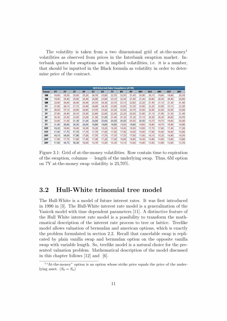
The volatility is taken from a two dimensional grid of at-the-money1

volatilities as observed from prices in the Interbank swaption market. In-terbank quotes for swaptions are in implied volatilities, i.e. it is a number,that should be inputted in the Black formula as volatility in order to deter-mine price of the contract.

Figure 3.1: Grid of at-the-money volatilities. Row contain time to expirationof the swaption, columns — length of the underlying swap. Thus, 6M optionon 7Y at-the-money swap volatility is 23,70%.

3.2 Hull-White trinomial tree model

The Hull-White is a model of future interest rates. It was first introducedin 1990 in [3]. The Hull-White interest rate model is a generalization of theVasicek model with time dependent parameters [11]. A distinctive feature ofthe Hull White interest rate model is a possibility to transform the math-ematical description of the interest rate process to tree or lattice. Treelikemodel allows valuation of bermudan and american options, which is exactlythe problem formulated in section 2.2. Recall that cancelable swap is repli-cated by plain vanilla swap and bermudan option on the opposite vanillaswap with variable length. So, treelike model is a natural choice for the pre-sented valuation problem. Mathematical description of the model discussedin this chapter follows [12] and [6].

1“At-the-money” option is an option whose strike price equals the price of the under-lying asset. (S0 = Sk)

11

3.2.1 Interest rate equation

Consider a mathematical representation of the model. Interest rate evolvesaccording to the equation:

dr = (Θ (t)− α (t) r) dt+ σ (t) dV (t) (3.3)

Where Θ (t) is a deterministic function of time. The function Θ (t) isused for adjustment of the Hull-White interest rate model to the currentterm structure. In other words, Θ (t) is calibrated to prices of zero-couponbonds that are equivalent to pure discount factors. In turn, parameters α andσ enable model to fit market volatility structure. This implies calibrating themodel against market prices of relevant instruments (depending on valuationpurposes of the model) by exhaustion of parameters α and σ.

Let us solve for r (t). Differentiate 3.3:

d(eatr

)= aeatrdt+ eatdr (3.4)

Insert 3.3 to the rhs of 3.4:

aeatrdt+ eatdr = aeatrdt+ eatΘ (t) dt− aeatrdt+ eatσdW

Integrate.

eatr (t)− r (0) =

∫ t

0

easΘ (s) ds+ σ

∫ t

0

easdW (s) ,

r (t) = e−atr (0) +

∫ t

0

ea(s−t)Θ (s) ds+ σ

∫ t

0

ea(s−t)dW (s) ,

r (t) = ψ (t)+σ

∫ t

0

ea(s−t)dW (s) , where ψ (t) = e−atr (0)+

∫ t

0

ea(s−t)Θ (s) ds

Add ∆t.

r (t+ ∆t) = ψ (t+ ∆t) + σ

∫ t+∆t

0

ea(s−t−∆t)dW (s) ,

r (t+ ∆t)− e−a∆tr (t) = ψ (t+ ∆t)− e−a∆tψ (t) + σ

∫ t+∆t

0

ea(s−t−∆t)dW (s) ,

(3.5)The Ito stochastic integral is defined as Yt =

∫ t0HsdXs, where X is

a Brownian motion. This is exactly the third term of the rhs of 3.5 —σ∫ t+∆t

0ea(s−t−∆t)dW (s). Thus, by the property of Ito stochastic integral it

12

is a normally distributed stochastic variable with mean zero and varianceequal to:

σ2

∫ t+∆t

0

e2α(s−t−∆t)dW (s) =σ2

2α

[1− e2a∆t

].

Hence,r (t+ ∆t) = ea∆tr (t) + h (t)Zt,

where h2 (t) = σ2

2α

[1− e2a∆t

]r (t+ ∆t) = r (t) +

(e−α∆t − 1

)︸ ︷︷ ︸M

r (t) + h (t)Zt. (3.6)

3.2.2 Converting to tree process

Now it is time to transform mathematical interest rate dynamics expressioninto tree lattice. Recall equation 3.6. Standard normal distribution can bediscretized to a 3-points distribution by expressing its first five moments inthe following way:

E[1] = Pa + Pb + Pc = 1

E[z] = aPa + bPb + cPc = 0

E[z2] = a2Pa + b2Pb + c2Pc = 1

E[z3] = a3Pa + b3Pb + c3Pc = 0

E[z4] = a4Pa + b4Pb + c4Pc = 3

E[z5] = a5Pa + b5Pb + c5Pc = 0

Solving the systems of equations gives:

a = −√

3, b = 0, c =√

3, Pa = 1/6, Pb = 2/3, Pc = 1/6.

In order to obtain a recombining tree2 one must put the following con-straints on r(t+ ∆t)− r(t):

Mr(t) + h(t)Zt =

−h(t)

√3

0

h(t)√

3

2A recombining tree is a tree in which a down move followed by an up one is equivalentto an up move followed by a down one.

13

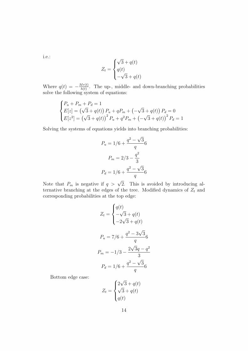
i.e.:

Zt =

√

3 + q(t)

q(t)

−√

3 + q(t)

Where q(t) = −Mr(t)h(t)

. The up-, middle- and down-branching probabilitiessolve the following system of equations:

Pu + Pm + Pd = 1

E[z] =(√

3 + q(t))Pu + qPm +

(−√

3 + q(t))Pd = 0

E[z2] =(√

3 + q(t))2Pu + q2Pm +

(−√

3 + q(t))2Pd = 1

Solving the systems of equations yields into branching probabilities:

Pu = 1/6 +q2 −

√3

q6

Pm = 2/3− q2

3

Pd = 1/6 +q2 −

√3

q6

Note that Pm is negative if q >√

2. This is avoided by introducing al-ternative branching at the edges of the tree. Modified dynamics of Zt andcorresponding probabilities at the top edge:

Zt =

q(t)

−√

3 + q(t)

−2√

3 + q(t)

Pu = 7/6 +q2 − 3

√3

q6

Pm = −1/3− 2√

3q − q2

3

Pd = 1/6 +q2 −

√3

q6

Bottom edge case:

Zt =

2√

3 + q(t)√3 + q(t)

q(t)

14

Pu = 1/6 +q2 +

√3

q6

Pm = −1/3− 2√

3q + q2

3

Pd = 7/6 +q2 + 3

√3

q6

3.2.3 Tree consistency with market term structure

An adjustment procedure was first introduced by Hull and White in [6]. Theysuggested adding the function g(t)to the r(t) process at each node. Recallthat g(t) is a function of θ(t) and selection of θ(t) enables the model to fitthe term structure. In other words, nodes of the tree are adjusted in orderto correctly price zero-coupon bonds at all maturities, or, what is equivalent,provide correct discount factors.

Firstly, prices of benchmark securities are determined. In this particularcase zero-coupon bond is the benchmark. For every time moment at whichtree nodes are placed zero-coupon price is calculated, which is, essentially, thesame as a discount factor. Discount factors are computed from the discount-ing yield curve according to simple discounting formulas. It is D = e−rt incase of continuous compounding, for example. This is one part of adjustingequation.

Another one is a price of the same security given by the tree model. Note,that adjusting process g(t) added to the tree at time node t will affect allsubsequent cash flows. Thus, a recursive expression that allows to expressthe price of security that pays 1 money unit at time ti depending on theprice of the same security at time ti−1 is needed. For these purposes conceptof Arrow-Debreu prices is used. The concept was introduced in [13] andsince [14] is used in financial economics. The Arrow-Debreu price is a priceof security that pays 1 money unit if a specific condition is fulfilled and 0otherwise. In our case, the condition is reaching by the interest rate processa specific node of the tree, node hk for instance. Moreover, in order to keeprecursiveness we incorporate condition on previous state of the interest rateprocess, i.e. a price of the security at node hk on condition that node ij wasreached on the previous step. Let us denote Arrow-Dbreu price as Q, valueof the security as V and cash flow as C. Then:

V (h, k) =∑i>k

∑j

Q (i, j|h, k)Ci,j

15

where,Q (i, j|h, k) = p (i, j|i− 1, k) e−ri−1,k(ti−ti−1)

and p (i, j|i− 1, k) denotes a conditional probability of reaching node j onstep i being at node k on step i − 1. The summation is taken over all timemoments i which follow time moment k and all nodes at particular time stepi. Hence, the price of zero-coupon bond, or a discount factor can be expressedas following:

Pi+1 =∑i

Qi,je−f(ri,j+gi)(ti+1−ti)

where:

gi =ln[∑

j Qi,je−fi(ri,j)∆ti

]− ln (Pi+1)

∆ti

which is the adjustment process at time moment i. It remains only to note,that since Q0,0 = 1 the value of g0 equals the initial ∆t0 interest rate.Finally, the recursive process is continued for every ti and computed adjust-ment process g(t) is added to the interest rate process r(t).

On completion of adjustment process constructed tree is consistent withrespective term structure and branching process produces correct discountfactors.

However, it is time to mention one of the main HW trinomial tree modelspitfalls. Unfortunately, the HW model can lead to negative rates. Adjust-ment process has no built-in protection against negative interest rates. Inorder to guarantee mean-reversion and recombining property we must acceptthe fact that negative interest rates can appear in the tree branching process.The risk of negative rates is even higher when market implies low interestrates as nowadays (2012).

3.2.4 Calibration

The final stage of tree construction is calibration. Like adjustment, cali-bration refines model parameters in such a way that the model producesresults consistent with real life phenomena. But in contrast to adjustment,calibration process is not so definite. There is no all-purpose instrumentin compliance with which volatility structure is calibrated. Theory, marketpractice and intuition suggest to use instruments as similar as possible tothe one is being priced. In addition, target instruments should be sufficientlyliquid to represent current market conditions.

In this paper the tree is calibrated to European swaptions volatility grid,which was described in section 3.1. There is no instrument available on the

16

market that is more close to cancelable swap and in the same time has quotesin volatility then European swaption.

Calibration is a problem of optimization. Levenberg-Marquardt algo-rithm is used to find set of volatilities that minimizes the sum of the squaresof the difference between the model price and market price of European swap-tions. It is worth to mention, that the same method is used for built-in treescalibration routines in Matlab.

3.3 Constructing a yield curve

The first step in valuation of any kind of financial contract is constructionof a yield curve. The yield or discounting curve is constructed from relevantinstruments quotes currently available on the market. The quote rates curveis a raw material from which a zero coupon yield curve is derived usuallyusing a method called “bootstrapping”. This involves deriving each newpoint on the curve from previously determined zero coupon points. Beyonda shadow of a doubt, problem of yield curve construction is worth anotherthesis. This section presents methodology according to which zero-couponyield curve for purposes of this paper was constructed.To begin with, one must determine a set of instruments from which the curvewill be constructed. In case of pricing cancelable swaps, zero-coupon curveis used for discounting of swap cash flows. Therefore, it was decided to usethe following set of instruments:

• Overnight deposit as the most liquid and riskless instrument currentlyavailable on the market.

• STIBOR Index as the most common floating leg index on the Swedishmarket.

• Floating rate notes (FRN) as allied to swaps instruments. Swap con-tracts are usually replicated by a portfolio of FRN.

• Plain vanilla interest rate swaps in SEK.

General algorithm of curve derivation:

1 First calculate the discount factor, DF, using par rates, pr, from shortterm instruments (overnight deposit and STIBOR) using the formulaDF = 1

1+(pr/100)∗Ndays

2 Using DF calculate zero coupon rate, rz, according to formula rz =−100ln(DF )Ndays/365

17

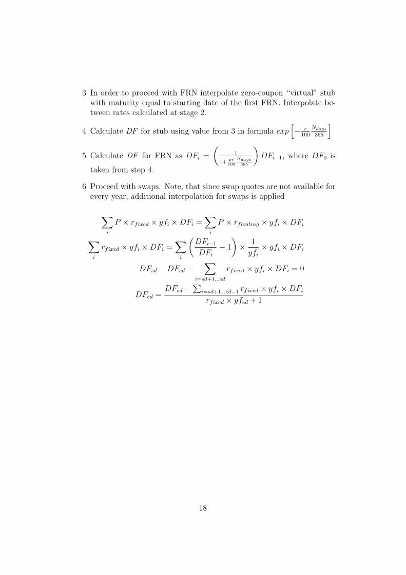
3 In order to proceed with FRN interpolate zero-coupon “virtual” stubwith maturity equal to starting date of the first FRN. Interpolate be-tween rates calculated at stage 2.

4 Calculate DF for stub using value from 3 in formula exp[− r

100

Ndays

365

]5 Calculate DF for FRN as DFi =

(1

1+ pr100

Ndays365

)DFi−1, where DF0 is

taken from step 4.

6 Proceed with swaps. Note, that since swap quotes are not available forevery year, additional interpolation for swaps is applied

∑i

P × rfixed × yfi ×DFi =∑i

P × rfloating × yfi ×DFi

∑i

rfixed × yfi ×DFi =∑i

(DFi−1

DFi− 1

)× 1

yfi× yfi ×DFi

DFsd −DFed −∑

i=sd+1...ed

rfixed × yfi ×DFi = 0

DFed =DFsd −

∑i=sd+1...ed−1 rfixed × yfi ×DFirfixed × yfed + 1

18

Chapter 4

Model implementation

Overview of the developed application and valuation results are presented inthis section.

4.1 Overview of the developed application

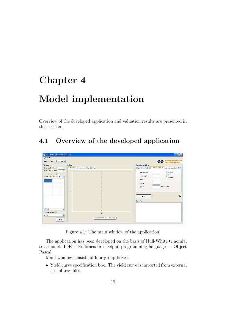
Figure 4.1: The main window of the application.

The application has been developed on the basis of Hull-White trinomialtree model. IDE is Embracadero Delphi, programming language — ObjectPascal.

Main window consists of four group boxes:

• Yield curve specification box. The yield curve is imported from external.txt of .csv files.

19

• Output tab panel. This panel contains charts of yield curve and cali-bration output information. Tree viewer tab presents an interest ratelattice in matrix form.

• Valuation section is a tab panel which contains controls for specificationof different instruments.

• Console panel. Various additional information is represented in theconsole (for example error and warning messages).

Subproducts of cancelable swaps solutions can be used for valuation of lesscomplex instruments. Indeed, calculation of discount factor is equal to valu-ating a zero coupon bond. Tree calibration routine involves fitting the modelto market prices of European style swaptions. Cancelable swap is replicatedwith plain-vanilla swap and bermuda style variable swaption. So, applicationdeveloped for purposes of this paper allows user to valuate following types ofinstruments:

• Bonds:

Zero-coupon bond;

Coupon bond;

Callable/Putable bond.

• Bond option:

European;

American.

• Swaption:

European;

American.

• Cancelable Swap.

4.2 Valuation

In this section valuation of existing cancelable swap contract is presented.Contract details were kindly provided by Swedbank. The presented interestrate swap was set up between Swedbank and another major European bankin May 2011.

20

Contract details:Start date : 2011 31 MayMaturity date : 2026 31 MayType : payerNotional : 20 000 000.00Currency : SEKIndex : STIBORSpread : 0Fixed rate : 1.45%

2.90%Payments per year : 4Cancellable from : 2013 31 MayCancellation dates : as payment dates

The valuation date is 2011 Nov 09.

4.2.1 Constructing the tree

We construct the tree in such a way that nodes are placed at payment dates.As each leg of the contract under consideration has 4 resets per year, nodesof the tree are evenly spaced each quarter (except of the first one). Time inthe model is represented as a fraction of year. Year fraction between Nov 092011 and Feb 29 2012 is 0.0575, so first node is placed 0.0575 years from now.Each following node is placed 0.25 years from the preceding one. The yearfraction between valuation date and maturity date is 14,5575 years whichis exactly the same as 0, 0575 + 0, 25 · 58 = 14, 5575 Next step is to load a

Figure 4.2: Tree construction dialog.

21

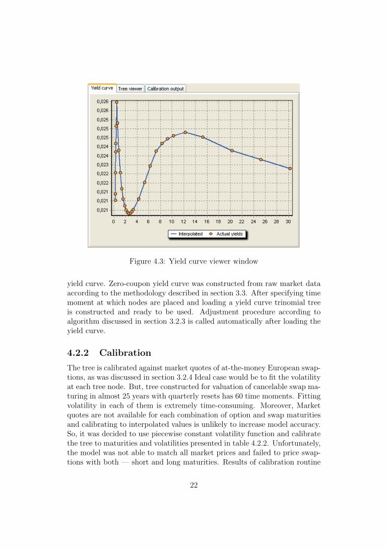
Figure 4.3: Yield curve viewer window

yield curve. Zero-coupon yield curve was constructed from raw market dataaccording to the methodology described in section 3.3. After specifying timemoment at which nodes are placed and loading a yield curve trinomial treeis constructed and ready to be used. Adjustment procedure according toalgorithm discussed in section 3.2.3 is called automatically after loading theyield curve.

4.2.2 Calibration

The tree is calibrated against market quotes of at-the-money European swap-tions, as was discussed in section 3.2.4 Ideal case would be to fit the volatilityat each tree node. But, tree constructed for valuation of cancelable swap ma-turing in almost 25 years with quarterly resets has 60 time moments. Fittingvolatility in each of them is extremely time-consuming. Moreover, Marketquotes are not available for each combination of option and swap maturitiesand calibrating to interpolated values is unlikely to increase model accuracy.So, it was decided to use piecewise constant volatility function and calibratethe tree to maturities and volatilities presented in table 4.2.2. Unfortunately,the model was not able to match all market prices and failed to price swap-tions with both — short and long maturities. Results of calibration routine

22

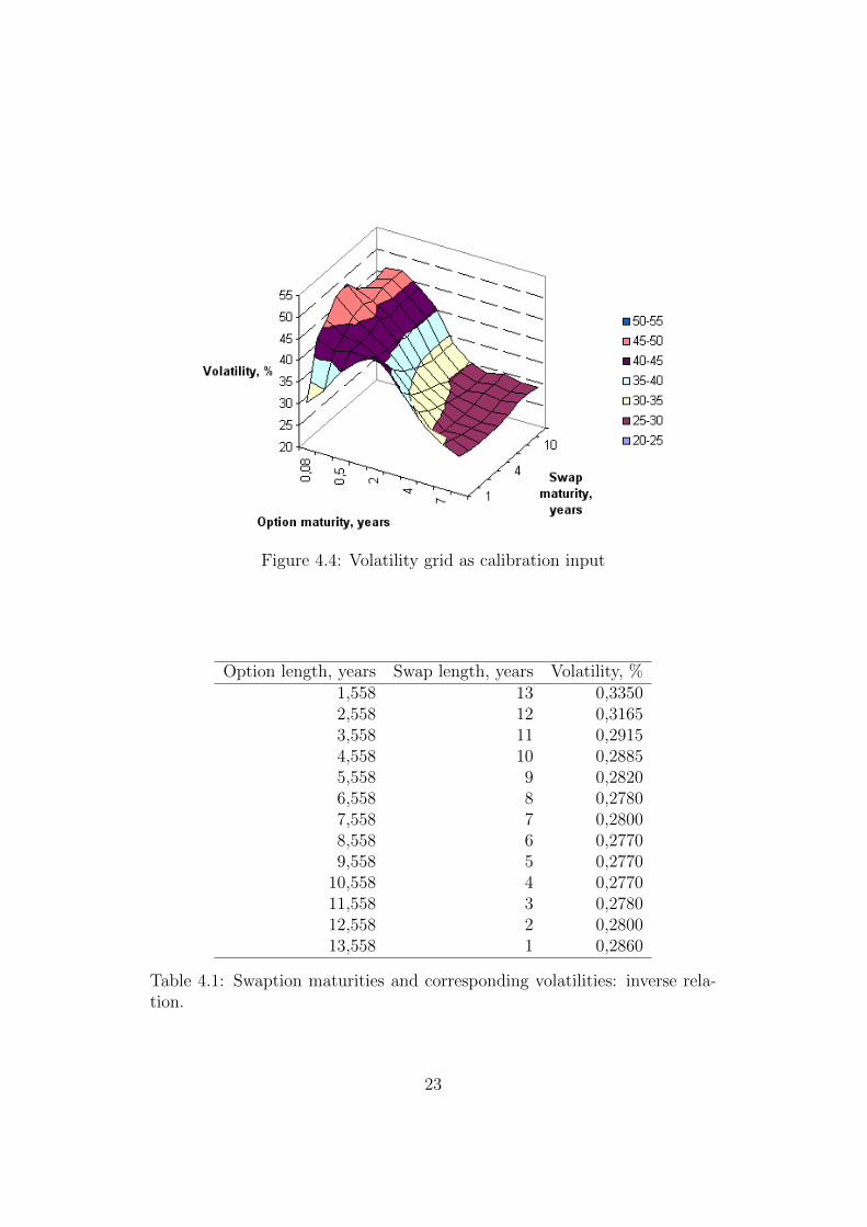
Figure 4.4: Volatility grid as calibration input

Option length, years Swap length, years Volatility, %1,558 13 0,33502,558 12 0,31653,558 11 0,29154,558 10 0,28855,558 9 0,28206,558 8 0,27807,558 7 0,28008,558 6 0,27709,558 5 0,2770

10,558 4 0,277011,558 3 0,278012,558 2 0,280013,558 1 0,2860

Table 4.1: Swaption maturities and corresponding volatilities: inverse rela-tion.

23

are displayed on Figure 4.5

Figure 4.5: Calibration output.

Figure 4.6: Sigma volatility parameter

According to the figure 4.5, the model failed to fit all market volatili-ties. Prices of swaptions with maturities from 6 to 10 years were fitted withgreat accuracy. But, the model was unable to fit both short and long termvolatilities. There can be several explanations of such outcome. The easiestway is to blame the calibration method, but it is not a case in this paper.Levenberg-Marquardt non-linear least square method is a trustworthy one

24

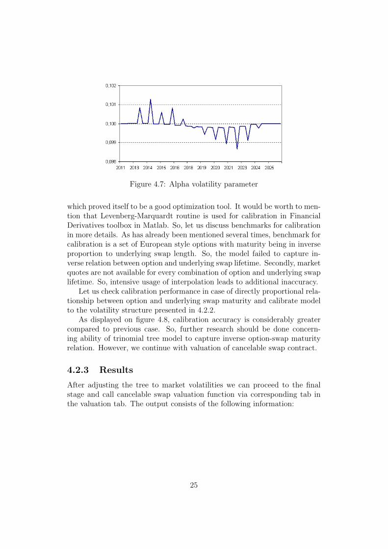
Figure 4.7: Alpha volatility parameter

which proved itself to be a good optimization tool. It would be worth to men-tion that Levenberg-Marquardt routine is used for calibration in FinancialDerivatives toolbox in Matlab. So, let us discuss benchmarks for calibrationin more details. As has already been mentioned several times, benchmark forcalibration is a set of European style options with maturity being in inverseproportion to underlying swap length. So, the model failed to capture in-verse relation between option and underlying swap lifetime. Secondly, marketquotes are not available for every combination of option and underlying swaplifetime. So, intensive usage of interpolation leads to additional inaccuracy.

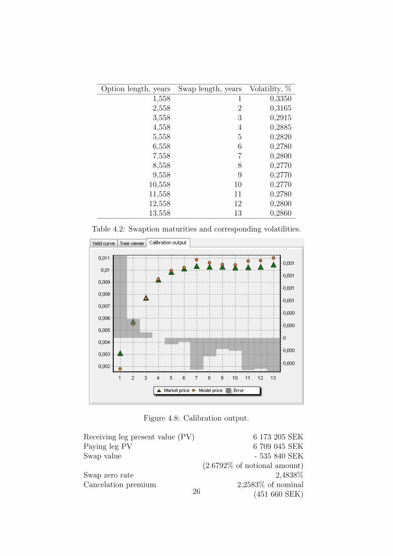
Let us check calibration performance in case of directly proportional rela-tionship between option and underlying swap maturity and calibrate modelto the volatility structure presented in 4.2.2.

As displayed on figure 4.8, calibration accuracy is considerably greatercompared to previous case. So, further research should be done concern-ing ability of trinomial tree model to capture inverse option-swap maturityrelation. However, we continue with valuation of cancelable swap contract.

4.2.3 Results

After adjusting the tree to market volatilities we can proceed to the finalstage and call cancelable swap valuation function via corresponding tab inthe valuation tab. The output consists of the following information:

25

Option length, years Swap length, years Volatility, %1,558 1 0,33502,558 2 0,31653,558 3 0,29154,558 4 0,28855,558 5 0,28206,558 6 0,27807,558 7 0,28008,558 8 0,27709,558 9 0,2770

10,558 10 0,277011,558 11 0,278012,558 12 0,280013,558 13 0,2860

Table 4.2: Swaption maturities and corresponding volatilities.

Figure 4.8: Calibration output.

Receiving leg present value (PV) 6 173 205 SEKPaying leg PV 6 709 045 SEKSwap value - 535 840 SEK

(2.6792% of notional amount)Swap zero rate 2,4838%Cancelation premium 2,2583% of nominal

(451 660 SEK)26

Obtained results were compared to valuation kindly provided by Swed-bank which is illustrated on figure 4.9. As can be observed on the graph:

• Present value of floating leg cash flows are perfectly correlated withcorrelation coefficient ≈ 0.99;

• There is constant spread between two floating cash flows series withaverage ≈ 3000 SEK per cashflow and standard deviation of 1500 SEK.

We would like to propose the following explanation of the nature of thisspread. As recent financial crisis has shown, even such big financial institu-tions as major international investment banks can go into default during ashort period of time. So perception of what is risk-free has changed drasti-cally. This resulted in evolution of risk-spread models. Yield curve whichhas been constructed for purposes of this paper does not account for counter-party risk and uses no risk adjustments spread. This facts results in parallelshift between model presented in this paper and Swedbank valuation model.Counterparty risk and risk-spread adjustment is a topic sufficient for anotherbunch of papers and is beyond a scope of this paper. We treat the yield curveas input information for the Hull-White trinomial tree model, and there canbe numerous ways of input information definition according to particularcircumstances.

Figure 4.9: Present value of swap cash flows

27

4.2.4 Cancellation premium

As was mentioned in section 2.2, cancellation premium can be expressed intwo equivalent forms: either as a single cash flow or being incorporated intofixed rate. In this section in the previous subsection cancellation premiumhas been determined as a single cashflow as the contract under considerationhas been already started with all parameters specified already. But, if partiesare about to enter a new cancelable swap contract then cancellation premiumis incorporated into a fixed rate, making it higher or lowering depending onwhich party has a right of cancellation. Let us discuss how cancellationpremium adjusts fixed rate in more details.

On the initiation date interest rate swap is set in such a way, that it’spresent value is 0. This condition means that present value of both legs areequal:

Nrf

n∑i=1

(tiTiD(ti)

)= N

m∑j=1

(fjtjTjD(tj)

)(4.1)

Where N denotes notional amount (can be canceled), n and m — number ofcash flows on fixed and floating legs respectively, rf — fixed rate and D(t) isa discount actor which corresponds to time moment t, fj — forward rate andTi is the time basis selected according to the specific day count convention.In addition, let us denote premium for cancellation as Pc. Thereafter, fixedrate is easily solved from 4.1:

rf =

∑mj=1

(fj

tjTjD(tj)

)∑n

i=1

(tiTiD(ti)

)Now, consider two cases:

1 Fixed rate payer party receives a right to terminate the contract atsome predefined date and Pc (expressed in % of N) has already beencalculated. Equation 4.1 must still hold, but now with Pc taken intoaccount:

rf

n∑i=1

(tiTiD(ti)

)=

m∑j=1

(fjtjTjD(tj)

)+ Pc

rf =

∑mj=1

(fj

tjTjD(tj)

)+ Pc∑n

i=1

(tiTiD(ti)

)Where Pc ≥ 0 by definition. Thus, for fixed rate payer party thepossibility to terminate the contract results in paying higher fixed rate.

28

2 An opposite case: floating rate payer party can annul the swap. Ex-pression 4.1 becomes:

rf

n∑i=1

(tiTiD(ti)

)+ Pc =

m∑j=1

(fjtjTjD(tj)

)

rf =

∑mj=1

(fj

tjTjD(tj)

)− Pc∑n

i=1

(tiTiD(ti)

)what results in receiving lower fixed interest rate in comparison toplain-vanilla swap.

29

Chapter 5

Conclusions

In this paper the problem of valuation of cancelable swaps via Hull-Whitetrinomial tree model has been investigated. Results of this study can besummarized as follows:

• Valuation of cancelable swap contract performed in this paper is consis-tent with Swedbank internal one. Correlation between cash flow seriesobtained in this paper and the one provided by Swedbank is 0.99. Meandifference is ≈ 3000 SEK per cashflow, and standard deviation ≈ 1500SEK. Premium for cancellation has been determined to be 2,2583 % ofnotional amount.

• During the calibration the model failed to capture inverse relationshipbetween maturities of swaption and underlying swap, fitting only abouta half of benchmark prices . However, calibration with directly propor-tional relationship worked fine. So, we suggest to perform more testson calibration problem trying different optimization methods.

• The constant shift between cash flows obtained in this study and pro-vided by Swedbank can be explained by adding risk spread to the dis-counting yield curve. The yield curve adjustment is dependent on par-ticular counterparty and this question is as well of great interest. Wesuggest it as another area of further research.

• One of Hull-White trinomial tree model pitfalls is generating of nega-tive interest rates on the bottom nodes of the tree. This phenomenaoccurs during extremely volatile and low interest rate market, which isobserved nowadays: interest rates are low and uncertainty about sol-vency of financial institutes and even states is high. In order to fulfillHull-White trinomial tree model assumptions and properties we have

30

to accept negative interest rates phenomena. More studies should beperformed on compensation or adjustment of negative interest ratesalgorithms.

• Developed application provides the user with comfortable GUI for work-ing not only with cancelable swaps, but also with swaptions of europeanand american style, bonds and bond options.

31

Bibliography

[1] Patrick S. Hagan. Methodology for callable swaps and bermudan ”ex-ercise into” swaptions.

[2] Mercurio Fabio Brigo Damiano. Interest Rate Models - Theory andPractice. Corr. 3rd printing, 2006, LVI, 981 p. 124 illus., 2006.

[3] John Hull and Alan White. Pricing interest-rate-derivative securities.The Review of Financial Studies, 3(4):pp. 573–592, 1990.

[4] J. Hull and A. White. Numerical procedures for implementing termstructure models i: Single-factor models. Journal of Derivatives, 2, 1:7–16, 1994.

[5] J. Hull and A. White. Numerical procedures for implementing termstructure models ii: Two-factor models. Journal of Derivatives, 2, 1:37–48, 1994.

[6] John Hull and Alan White. The general hull-white model and supercalibration. Journal of Derivatives, 2000.

[7] John C. Hull. Options, Futures, and Other Derivatives. Prentice Hall;8 edition, 2011.

[8] http://www.sdgm.com/support/glossary.aspx?term=cancelable

[9] Quarterly review. Technical report, The Bank for International Settle-ments, March 2012.

[10] Fischer Black. The pricing of commodity contracts. Journal of FinancialEconomics, 3:167–179, 1976.

[11] Jan R. M. Roman. Lecture notes in analytical finance ii. 2011.

[12] Valentino Grassi Mattia Carlo Diego Ferrini. Pricing plain-vanilla andexotic callable bonds. Master’s thesis, Kungliga Tekniska Hogskolan,2006.

32

[13] K. J. Arrow G. Debreu. Existence of an equilibrium for a competitiveeconomy. Econometrica, 22:265–290, 1954.

[14] Robert H. Litzenberger Douglas T. Breeden. Prices of state-contingentclaims implicit in option prices. The Journal of Business, 51, 4, 1978.

33

List of Figures

2.1 Cancelable swap mechanism. . . . . . . . . . . . . . . . . . . . 72.2 Interest rate contracts market volume dynamics. . . . . . . . . 8

3.1 European swaptions volatility grid . . . . . . . . . . . . . . . . 11

4.1 The main window of the application. . . . . . . . . . . . . . . 194.2 Tree construction dialog. . . . . . . . . . . . . . . . . . . . . . 214.3 Yield curve viewer window . . . . . . . . . . . . . . . . . . . . 224.4 Volatility grid as calibration input . . . . . . . . . . . . . . . . 234.5 Calibration output. . . . . . . . . . . . . . . . . . . . . . . . . 244.6 Sigma volatility parameter . . . . . . . . . . . . . . . . . . . . 244.7 Alpha volatility parameter . . . . . . . . . . . . . . . . . . . . 254.8 Calibration output. . . . . . . . . . . . . . . . . . . . . . . . . 264.9 Present value of swap cash flows . . . . . . . . . . . . . . . . . 27

34

List of Tables

2.1 Types of swaption contracts . . . . . . . . . . . . . . . . . . . 62.2 Interest rate contracts market volume dynamics. . . . . . . . . 8

4.1 Swaption maturities and corresponding volatilities: inverse re-lation. . . . . . . . . . . . . . . . . . . . . . . . . . . . . . . . 23

4.2 Swaption maturities and corresponding volatilities. . . . . . . 26

35