Master Thesis Extended GN Model for L-C Band with final ...
103
Master Thesis Extended GN Model for L-C Band with final experimental verifications Double Degree Program MSc Communications and Computer Networks Engineering M´ aster Universitario en Ingenier´ ıa de Telecomunicaci´ on ´ Angel Alonso G´ omez Supervisors: Prof. Dr. Andrea Carena Prof. Dr. Luis Salgado Company Supervisor: Dr. Antonio Napoli 2
Transcript of Master Thesis Extended GN Model for L-C Band with final ...

Master Thesis
Extended GN Model for L-C Band with final
experimental verifications
Double Degree Program
MSc Communications and Computer Networks Engineering
Master Universitario en Ingenierıa de Telecomunicacion
Angel Alonso Gomez
Supervisors:
Prof. Dr. Andrea Carena
Prof. Dr. Luis Salgado
Company Supervisor:
Dr. Antonio Napoli
2


Abstract
Nowadays, the huge data traffic growth has forced telecommunications companiesand vendors to deploy ultra-wideband optical systems. To do so, they need of toolsthat allow them to estimate the system performance and to plan properly the op-tical network. On the physical layer, the metric used to characterize the systemperformance is the well-known Signal-to-Noise Ratio (SNR). This value determinesthe Quality of Transmission (QoT). Beyond of ASE noise impairments, the noise-like ”non-linear interference” (NLI) power is also a critical issue that should beconsidered. The goal of this project is to evaluate the well-known Gaussian NoiseModel (GN-Model) and the forefront version, the Generalized Gaussian Noise Model(GGN-Model)[1]. On the Introduction Chapter, the current state-of-the-art is brieflydescribed and which are the cutting-edge tools to estimate system performance, aswell as main optical fiber parameters involved on the non-linear interference gener-ation. On the second Chapter, the metric used to defined the QoT is explained andthrough this value, the system performance is estimated. The metric is basicallythe SNR as it was introduced earlier. Following what was set forth above, the noisepower is not only composed of ASE noise power, but also of noise-like NLI power.On the third Chapter, the GN-Model is thoroughly described as well as its physicalmeaning. Some important results came out after comparing how the noise-like NLIpower is piled up varying system parameters (frequency spacing, number of spansetc). 50% of total noise-like NLI power is agglomerated between 3-7 channels (it de-pends on the number of spans and other system parameters). Furthermore, it wasreported that the smaller the frequency spacing, the more incoherent is the non-linear e↵ect accumulation. Incoherent accumulation symbolize that the noise-likeNLI power generated on one span is summed up in power with the contributions ofthe rest of spans. On the fourth Chapter, the GGN-Model derivation is deeply ex-plained. Main improvements with respect to GN-Model are considered as well. Onthe fifth Chapter, the model implementation and how all files interact each others isclarified. Finally on the sixth Chapter, all tests and simulations carried out throughthis thesis are illustrated. The most important one is the full C-Band (191.35-196THz) + 15 Channels on L-Band (190.2-190.9 THz) without tilt compensation. Theperformance on a channel, placed on the lowest side of the operating bandwidth,is reported to be 7 dB worst than that obtained on a channel, placed on the high-est side of the operating bandwidth in terms of frequency. Moreover, it has beendemonstrated, how GN-Model reports mistaken estimates on L-Band for L+C sys-tem without Stimulated Raman Scattering (SRS) cross-talk compensation. Indeed,a di↵erence of approximately 2000 km is reported in terms of maximum distancegiven a certain Bit Error Rate requirement (BER).
Key Words— GN-Model, GGN-Model, C+L systems, Matlab, Ultra wide-bandOptical Networks, OSNR, SNR, SRS and BER

Dedicado ami familia.
1
Contents
1 Introduction and Coherent Optical Systems 71.1 Scenario under Analysis . . . . . . . . . . . . . . . . . . . . . . . . . 81.2 Fiber Loss. Attenuation Coefficient . . . . . . . . . . . . . . . . . . . 91.3 Chromatic Dispersion Parameter . . . . . . . . . . . . . . . . . . . . 101.4 Kerr E↵ect . . . . . . . . . . . . . . . . . . . . . . . . . . . . . . . . 111.5 Raman Scattering. Raman Cross-Talk . . . . . . . . . . . . . . . . . 12
2 Gaussian Noise Model 152.1 GN-Model Reference Formula . . . . . . . . . . . . . . . . . . . . . . 152.2 Physical Interpretation of the GN-Model . . . . . . . . . . . . . . . . 162.3 FWM E↵eciency Factor . . . . . . . . . . . . . . . . . . . . . . . . . 172.4 Coherent Accumulation Factor . . . . . . . . . . . . . . . . . . . . . . 182.5 Hyperbolic Coordinates . . . . . . . . . . . . . . . . . . . . . . . . . . 182.6 GN-Model Approximated Formula . . . . . . . . . . . . . . . . . . . . 202.7 NLI Accumulation . . . . . . . . . . . . . . . . . . . . . . . . . . . . 21
3 Generalized Gaussian Noise Model 233.1 Generalized GN-Model Reference Formula . . . . . . . . . . . . . . . 233.2 FWM Efficiency Factor . . . . . . . . . . . . . . . . . . . . . . . . . . 31
4 Metric to assess Quality of Transmission (QoT) 344.1 Metric definition and GN-Model implications . . . . . . . . . . . . . . 344.2 Maximum Length . . . . . . . . . . . . . . . . . . . . . . . . . . . . . 36
5 Model implementation 385.1 Code Structure . . . . . . . . . . . . . . . . . . . . . . . . . . . . . . 38
5.1.1 Fiber Parameters . . . . . . . . . . . . . . . . . . . . . . . . . 385.1.2 System-Signal Parameters . . . . . . . . . . . . . . . . . . . . 395.1.3 GN-Model Approximated Formula . . . . . . . . . . . . . . . 405.1.4 GN-Model Cartesian Coordinates . . . . . . . . . . . . . . . . 405.1.5 GN-Model Hyperbolic Coordinates . . . . . . . . . . . . . . . 415.1.6 GN-Model Hyperbolic Coordinates for f=0 . . . . . . . . . . . 415.1.7 GGN-Model Matrix Solution . . . . . . . . . . . . . . . . . . . 415.1.8 GGN-Model Loop/Matrix Solution . . . . . . . . . . . . . . . 425.1.9 GGN-Model Hybrid Solution . . . . . . . . . . . . . . . . . . . 42
2

CONTENTS
5.2 Code performance . . . . . . . . . . . . . . . . . . . . . . . . . . . . . 435.2.1 Hyperbolic Coordinates vs Cartesian Coordinates . . . . . . . 445.2.2 Generalized Gaussian Noise Model Matrix Solution . . . . . . 455.2.3 Generalized Gaussian Noise Model Loop/Matrix Solution . . . 465.2.4 Generalized Gaussian Noise Model Hybrid Solution . . . . . . 47
6 Experimental verification and simulations 486.1 Telecom Italia Field Trial . . . . . . . . . . . . . . . . . . . . . . . . 486.2 Maximum Distance GN-Model . . . . . . . . . . . . . . . . . . . . . . 516.3 Experiment at Orange Laboratory . . . . . . . . . . . . . . . . . . . . 52
6.3.1 Laboratory Setup . . . . . . . . . . . . . . . . . . . . . . . . . 526.3.2 Results and Conclusions . . . . . . . . . . . . . . . . . . . . . 53
6.4 Experiment at Coriant Laboratory. Full C-Band + 15 L-Band . . . . 566.4.1 Laboratory Setup . . . . . . . . . . . . . . . . . . . . . . . . . 566.4.2 Measurements and Conclusions . . . . . . . . . . . . . . . . . 59
6.5 15 Channels on C-Band and 35 Channels on L-Band . . . . . . . . . 63
7 Conclusions 65
Appendices 66
A Matlab Files 67
3
List of Figures
1.1 Multi-span Optical System Scenario [2] . . . . . . . . . . . . . . . . . 81.2 Coherent Transmission Modulator [3] . . . . . . . . . . . . . . . . . . 91.3 Blue solid line represent both ↵ and D for G.652A and orange solid
line represents ↵ for G.652D [4] . . . . . . . . . . . . . . . . . . . . . 101.4 Blue solid line represents the Raman Gain and red solid one represents
the triangular approximation . . . . . . . . . . . . . . . . . . . . . . . 131.5 Blue solid line input WDM Signal PSD and red solid line tilted WDM
Signal PSD due to SRS e↵ect . . . . . . . . . . . . . . . . . . . . . . 14
2.1 Red area represents the integration domain for MCI, yellow one doesthe XCI one and the blue one does the SCI one. . . . . . . . . . . . . 17
2.2 Clipping o↵ the integration beyond -30 dB makes the integrationdomain 75% smaller . . . . . . . . . . . . . . . . . . . . . . . . . . . 19
2.3 χ(⌫1, 0) and threshold equal to -30 dB . . . . . . . . . . . . . . . . . 202.4 Red solid line 50 GHz frequency spacing, green solid line 38.4 GHz
and yellow solid line 32 GHz . . . . . . . . . . . . . . . . . . . . . . . 212.5 Blue solid line Ns = 50, green solid line Ns = 20 and red line Ns = 1 22
3.1 Blue solid line real part of the complex exponential and red dashedlines field profile of pumps frequencies, when (f1 − f)(f2 − f) is low. . 31
3.2 Blue solid line real part of the complex exponential and red dashedlines field profile of pumps frequencies, when (f1 − f)(f2 − f) is high. 32
3.3 Blue solid line represents IGN2 and red dashed line represents IGGN
2 . . 33
4.1 Reference Bandwidth for SNR (Rs) and for OSNR (Bn) . . . . . . . . 354.2 Random example of the I/Q diagram provided by the receiver . . . . 364.3 Green solid line represents the maximum length for a linear system
given the input power and blue solid line does it for a non-linear system 37
5.1 Code Architecture . . . . . . . . . . . . . . . . . . . . . . . . . . . . 435.2 The graph shows the computing time of the GN-Model for di↵erent
number of channels.Blue solid line represents Cartesian Coordinatesapproach and red solid line does Hyperbolic Coordinates one. Carte-sian Coordinates approach is faster than Hyperbolic Coordinates oneuntil 10 channels. Beyond 10 channels is the other way around. . . . 44
4

LIST OF FIGURES
6.1 Field Trial Architecture. This figure has been taken from [5] (Fig. 1) 496.2 The optimal input power is 4 dBm, 3 dBm and 2 dBm for DP-4QAM,
DP-8QAM and DP-16QAM respectively. Dashed line represent GN-Model Approximated Formula with incoherent accumulation. Thismodel reports larger distances for both DP-4QAM and DP-8QAM,because for these mod. schemes the frequency spacing is higher, thenNLI accumulation is more coherent. For DP-16QAM scheme the fre-quency spacing is lower. . . . . . . . . . . . . . . . . . . . . . . . . . 51
6.3 Maximum length for di↵erent input powers. SMF-QPSK case . . . . 526.4 Red solid line represents the central channel, blue solid line left chan-
nel and yellow dashed line right one . . . . . . . . . . . . . . . . . . . 536.5 Red solid line represents the central channel, blue solid line left chan-
nel and yellow solid line right one. It is observed that equalizationstages are placed on 6th and 13th spans. . . . . . . . . . . . . . . . . 54
6.6 Red solid line represents the central channel, blue solid line left chan-nel and yellow solid line right one . . . . . . . . . . . . . . . . . . . . 55
6.7 Blue solid line represents GN-Model and green solid line representsGGN-Model. GN-Model reports an over estimation at 193.5 THzwith respect to GGN-Model and an under estimation at 194.5 THzwith respect to GGN-Model. . . . . . . . . . . . . . . . . . . . . . . . 55
6.8 Experiment Architecture . . . . . . . . . . . . . . . . . . . . . . . . . 566.9 Input 96 Channels C-Band . . . . . . . . . . . . . . . . . . . . . . . . 576.10 Input 15 Channels L-Band . . . . . . . . . . . . . . . . . . . . . . . . 576.11 Output 96 Channels C-Band after 5 spans . . . . . . . . . . . . . . . 596.12 Output 15 Channels L-Band after 5 spans . . . . . . . . . . . . . . . 596.13 Back-to-back measurements . . . . . . . . . . . . . . . . . . . . . . . 606.14 Span Block Diagram . . . . . . . . . . . . . . . . . . . . . . . . . . . 616.15 Blue solid line represents Strategy 1 and red solid line represents
Strategy 2. Yellow bars represent +/- 1 dB around the measuredvalue. In other words, an estimation inside the interval [xmeasured −1, xmeasured + 1] is accepted. . . . . . . . . . . . . . . . . . . . . . . . 62
6.16 Measure for channel at 193.75 THz. Square-like dots represents themeasurements of ⌘nl and solid red line the simulated one. 0.5 dBmaximum di↵erence among measurements is reported. . . . . . . . . 63
6.17 Blue solid line GGN-Model at 190.3 THz, blue dashed line GN-Modelat 190.3, green solid line GGN-Model at 191.8 THz and green dashedline GN-Model at 191.THz. Both models report similar values at191.8 THz.On the other hand, GN-Model fails at 190.3 THz. . . . . . 64
5

List of Tables
6.1 Main Experiment Parameters . . . . . . . . . . . . . . . . . . . . . . 496.2 Main Fiber Parameters . . . . . . . . . . . . . . . . . . . . . . . . . . 496.3 Back-to-back values in terms of OSNR and SNR . . . . . . . . . . . . 506.4 Main Fiber Parameters . . . . . . . . . . . . . . . . . . . . . . . . . . 576.5 System Parameters . . . . . . . . . . . . . . . . . . . . . . . . . . . . 586.6 Span Losses . . . . . . . . . . . . . . . . . . . . . . . . . . . . . . . . 586.7 BER-SNR . . . . . . . . . . . . . . . . . . . . . . . . . . . . . . . . . 63
6
Chapter 1
Introduction and Coherent OpticalSystems
The continuous growth of IP-traffic requires that telco companies increase the band-width capabilities in order to fulfill customer’s requirements. To cope with this, sys-tem vendors evolved their products from direct-detection to coherent detection thatallows to improve spectral efficiency and reaches. In coherent systems accumulateddispersion can be compensated through digital signal processing. This leads to de-ployment of uncompensated transmission (UT), which presents several benefits (e.g.better performance and no dispersion-managed links). This is one of the main rea-sons why current optical systems generation is based on this approach. One of themain parameters for telecommunication operators (to measure system performance)is the OSNR (Optical signal-to-noise-ratio), defined as the ratio between opticalsignal power and noise power, i.e. ASE noise, from the amplifiers. Besides the ASE,another parameter strongly influences the system performance, this is the noise-likepower induced by nonlinear e↵ects. These systems and their main e↵ects can beefficiently modeled, and thus the network performance can be estimated. The mostwidely used model is the so-called Gaussian Noise Model, that e↵ectively addressesthe impact of non-linear propagation. The GN-Model helps the Physical SimulationEnvironment (PSE) [6], which under the Telecom Infra Project ,Inc. (TIP), intendsto provide an Open-Source physical layer performance-predicting module or tool.
Historically, due to limitation in optical amplification, the common band fortransmission has been C-Band (1528-1566 nm). Thus, the Gaussian Noise Modelhas been only designed and, fully tested in this spectral region. With the availabilityof new optical amplifiers delivering gain beyond the C-Band, there is a growinginterest in deploying future system in the extended C+L band, spanning from 1530nm to 1600 nm. The goal of this project is to extend GN-Model to GGN-Model fora reliable application over the C+L band.
7

1.1. SCENARIO UNDER ANALYSIS
1.1 Scenario under Analysis
The Multi-span and Coherent Transmission scenario is organized like a typical com-munication system, i.e. it is composed of a transmitter, a channel and a receiver.As multi-span approach is followed, the channel white box brings together many”channels”. Figure 1.1 summarizes the scenario.
Figure 1.1: Multi-span Optical System Scenario [2]
Regarding the Coherent System, the modulator inside the transmitter is consti-tuted by four branches, two in-phase components and two quadrature components.This is the consequence of the coherent system approach, where the ”information” isnot on the amplitude, but on the phase of the signal. One of the two in-phase com-ponents represents the x-component and the other one the y-component. For thequadrature components occurs the same. In other words, the information is trans-mitted both along x-axis and y-axis (double polarization). Therefore, PM-QPSKtransmits four bits per symbol, meanwhile QPSK does two one per symbol. Figure1.2 illustrates modulator scheme.
8

1.2. FIBER LOSS. ATTENUATION COEFFICIENT
Figure 1.2: Coherent Transmission Modulator [3]
1.2 Fiber Loss. Attenuation Coefficient
The attenuation coefficient ↵ includes all sources of attenuation. It is variableagainst the frequency, which will have further implications later. The evolutionof the power along the optical fiber is explained by an exponential Law.
Pout = Pine−↵L (1.1)
↵(dB/km) ⇡ 4.343↵ (1.2)
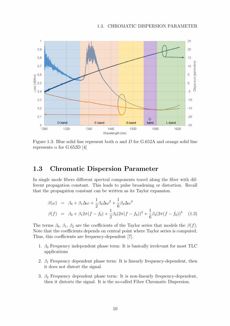
As it has been said before, the attenuation coefficient varies with the wavelength ofthe transmitted light. According to physical theory, the low-loss window is placedaround 1550 nm, where ↵ = 0.2 dB/km. This is the so-called C-Band. Nowadays,this region is the widely used bandwidth. However, both the needs of increasing thebandwidth and the improve on fiber manufacturing are making the usage of otherregion also interesting. For instance, L-Band has become quite interesting. On thisband the attenuation coefficient variation is more abrupt as in C-Band as it can beobserved on Figure 1.3
9
1.3. CHROMATIC DISPERSION PARAMETER
Figure 1.3: Blue solid line represent both ↵ and D for G.652A and orange solid linerepresents ↵ for G.652D [4]
1.3 Chromatic Dispersion Parameter
In single mode fibers di↵erent spectral components travel along the fiber with dif-ferent propagation constant. This leads to pulse broadening or distortion. Recallthat the propagation constant can be written as its Taylor expansion.
β(!) = β0 + β1∆! +1
2β2∆!
2 +1
6β2∆!
3
β(f) = β0 + β12⇡(f − f0) +1
2β2(2⇡(f − f0))
2 +1
6β3(2⇡(f − f0))
3 (1.3)
The terms β0, β1, β2 are the coefficients of the Taylor series that models the β(f).Note that the coefficients depends on central point where Taylor series is computed.Thus, this coefficients are frequency-dependent [7].
1. β0 Frequency independent phase term: It is basically irrelevant for most TLCapplications
2. β1 Frequency dependent phase term: It is linearly frequency-dependent, thenit does not distort the signal.
3. β2 Frequency dependent phase term: It is non-linearly frequency-dependent,then it distorts the signal. It is the so-called Fiber Chromatic Dispersion.
10

1.4. KERR EFFECT
The group velocity is the velocity at which the envelope of a set of optical pulsestravels through the fiber. The group velocity can be found using vg =
1β1. Further-
more, the β2 parameter represent dispersion of the group velocity and is responsiblefor pulse broadening. The group delay is defined as the delay experienced by aspectral component f compared to those at f0. The group delay is defined as
⌧g(f) = 2⇡β2(f − fo)L (1.4)
However, β2 is not the widely used parameter, but the dispersion parameter D. It isdefined as follows:
D =dβ1dλ
(1.5)
The dispersion parameter D has been defined in order to relate group delay (∆⌧g)variation with wavelength (λ). Then, Equation 1.4 can be re-defined as:
⌧g(λ) = ⌧g(λo) +D(λ− λo)L
∆⌧g = D∆λL (1.6)
And the dispersion parameter D is related with the group velocity dispersion (GVD)parameter β2:
D = −2⇡c
λ2β2 (1.7)
Both terms vanish at a wavelength around 1300 [nm] for pure silica fibers. Thiswavelength is called zero-dispersion wavelength and is denoted as λD. Finally, thetypical value is 16 [ps/nm/km] at 1550 [nm].
1.4 Kerr E↵ect
The Kerr e↵ect causes a variation in the glass refractive index, which depends onthe optical power P(z). It is the most important non-linear e↵ect on the fiber. Theconventional refractive index is defined as nL, n2 is the non-linear index coefficient,P(z,t) is the optical power and Aeff is the e↵ective area. However, the real refrac-tive index varies with time, as optical power does. Therefore an ”instantaneous”refractive index must be defined [8].
n(z, t) = nL + n2P (z, t)
Aeff
(1.8)
The e↵ective area can be approximated to the area where the optical mode in con-fined in the fiber. Then, it can be expressed as:
Aeff ⇡ ⇡r2 (1.9)
11

1.5. RAMAN SCATTERING. RAMAN CROSS-TALK
Where r is the core radius of the fiber.Since the refractive index and the propagation constant are related, a variation ofthe refractive index leads to a variation of the propagation constant.
∆β =2⇡
λ∆n
=2⇡
λn2
P (z)
Aeff
(1.10)
Then, the non-linear coefficient is defined:
γ =2⇡n2
λAeff
(1.11)
The Kerr E↵ect causes a phase shift induced by the signal power. This phase shiftis expressed as [8]
ΦNL(z, t) = −γ|E(0, t)|2zeff (1.12)
Here arises an important parameter in optical communications: the well-knowne↵ective length. It is defined as the length where the field amplitude only su↵ers aphase shift by the non-linearity (1.12).
zeff =1− e−2↵z
2↵(1.13)
1.5 Raman Scattering. Raman Cross-Talk
Raman Scattering is a physical phenomena that occurs when a photon interacts withthe propagation medium. The molecules, of which the guiding material is composed,can only oscillate at two energy levels, which are frequencies indeed. When thesesmolecules are excited by the incoming photon, they jump up to a higher level. How-ever, this energy level is prohibited. Therefore, they must jump down right after.As a result, if the final energy level is higher than the initial one, then less opticalpower is released together with the mechanical energy. On the other hand, if thefinal energy level is lower than the initial one, more mechanical energy is absorbedin order to release more optical energy as well [9].
There are two di↵erent kinds of Raman Scattering: The Spontaneous Raman Scat-tering and the Stimulated Raman Scattering (SRS). The former occurs in the ab-sence of incident photon, so that, new photons are generated. The latter does as aconsequence of an incoming photons flow. Therefore, energy from these photons istransferred to the propagating optical field. The most important e↵ect of RamanScattering are: Raman Cross-Talk, Raman Amplification and Raman Laser. BothRaman Amplification and Raman Laser are out os the scope of this thesis. We focuson Raman Cross-Talk e↵ect.
12

1.5. RAMAN SCATTERING. RAMAN CROSS-TALK
Raman Cross-Talk is a negative e↵ect of Raman Scattering that impairs theperformance of a WDM system. Higher frequency components transfers power tolower ones. As a results, the spectra is tilted. The e↵ect is governed by a setof discrete di↵erential equations [10]. Theses equation are based on the triangularapproximation to the Raman Gain spectrum. The triangular approximation assumesthat Raman Gain varies linearly until a certain cut-o↵ frequency (Typically 13.5THz). Figure 1.4 illustrates it.
@Pn(z)
@z+ ↵Pn(z) +
⇣g0∆f
2A
⌘Pn(z)
NX
m=1
(m− n)Pm(z) = 0 (1.14)
Figure 1.4: Blue solid line represents the Raman Gain and red solid one representsthe triangular approximation
In Equation (1.14), Pn(z) is the power of the nth channel as a function of thedistance z, ↵ is the power attenuation constant, g0 is the slope of the triangularapproximation to Raman gain, ∆f is the interchannel frequency spacing, A is thee↵ective area and Pm(z) is the power of the mth channel as a function of the distance.The 2 in the denominator represents the polarization averaging. The system ofdi↵erential equation exhibits the general solution:
Pn(z) = PnoJoe−↵zeGJ
o
(n−1)Ze
h NX
m=1
PmoeGJ
o
(m−1)Ze
i−1
(1.15)
In Equation (1.15), Pno is the input power of the nth channel, Jo is the total input
power and is defined as Jo =NP
m=1Pmo, G is the Raman gain G = g0∆
f
2A and Ze is the
13
1.5. RAMAN SCATTERING. RAMAN CROSS-TALK
e↵ective length Ze =1−e−↵z
↵.
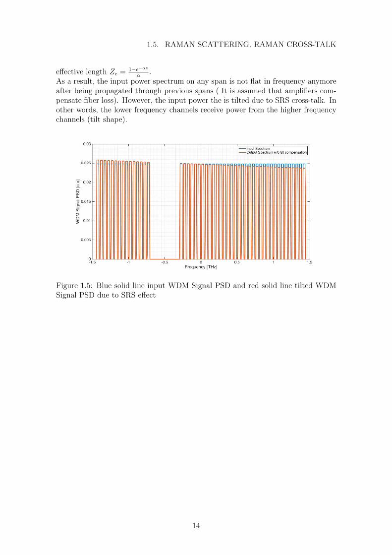
As a result, the input power spectrum on any span is not flat in frequency anymoreafter being propagated through previous spans ( It is assumed that amplifiers com-pensate fiber loss). However, the input power the is tilted due to SRS cross-talk. Inother words, the lower frequency channels receive power from the higher frequencychannels (tilt shape).
Figure 1.5: Blue solid line input WDM Signal PSD and red solid line tilted WDMSignal PSD due to SRS e↵ect
14

Chapter 2
Gaussian Noise Model
The Gaussian Noise Model aims at assessing the non-linear propagation and pro-viding a practical tool that allows to analyze system performance before deployingit. This model belongs to a family named as perturbation models [11]. The mainassumption is simply to consider non-linearity as a perturbation. In other words,the non-linear disturbance is considered relatively small. This has been proved towork at common optimal system launch power. Moreover, a second assumption isthat the transmitted signal behaves as a stationary Gaussian noise. Finally, thethird assumption is that the signal disturbance produced by the non-linearity e↵ectis assumed as Additive Gaussian Noise.
2.1 GN-Model Reference Formula
The Gaussian Noise Reference Formula, from now on GNFR Equation 1 [12], canbe written as follows:
GNLI(f) =16
27γ2L2
eff (Ls, f)2
ZZ 1
−1GWDM(f1)GWDM(f2)GWDM(f1 + f2 − f)
⇢(f1, f2, f)χ(f1, f2, f)df1df2 (2.1)
The symbols used are listed bellow:
1. γ: Kerr E↵ect Coefficient [W−1km−1]
2. Leff : E↵ective Length [km]
3. GWDM(f): WDM Signal Power Spectral Density [W/Hz]
4. ⇢(f1, f2, f): FWM Efficiency Factor
5. χ(f1, f2, f): Coherent Accumulation Factor
6. ↵: Attenuation Constant [1/km]
7. β2: Group Velocity Dispersion Factor [ps2/km]
15

2.2. PHYSICAL INTERPRETATION OF THE GN-MODEL
8. Ls: Span Length [km]
9. (Ls, f)2 Optical-Power Propagation function.
GNLI(f) is the NLI noise PSD. On the scientific literature (e.g. [12]), (Ls, f)2 isremoved. The reason comes from that it is the amount of power loss on the fiberand it is compensated by the amplifiers. Therefore, it depends on where GNLI(f) iscomputed, before or after the EDFA amplifier. The scenario of this chapter considersthat the fiber parameters does not change with neither frequency nor space, so that, (Ls, f)2 = e−2↵L
s .
2.2 Physical Interpretation of the GN-Model
Looking at the integral factor three actors are involved. Firstly, GWDM(f1)GWDM(f2)GWDM(f1 + f2 − f) represents the PSD of the three spectral components involvedin the Four-Wave Mixing process, which is an inter-modulation phenomenon thattakes place inside optical fibers. This process should be taken into account when theoptical fiber is considered a non-linear system. Two or three spectral componentsinteract each other and a new one is generated as a result. Secondly, ⇢(f1, f2, f) isthe non-degenerate FWM efficiency of their beating. Finally, χ(f1f2, f) is shown tobe the coherent accumulated factor that takes multiple spans into account and howNLI disturbance is being accumulated span after span. From the physical point ofview, the disturbance produced by the beating process can be classified in three kindof interference: SCI (Self-Channel Interference), XCI (Cross-Channel Interference)and MCI (Multiple-Channel Interference). The channel whose one of its frequencyis being analyzed is named channel under analysis.
1. Self-Channel Interference (SCI) All three spectral components (f1, f2 and f3)belongs to the channel under analysis.
2. Cross-Chanel Interference (XCI) It represents the interplay between the chan-nel under analysis and another channel
3. Multiple-Channel Interference (MCI) Each triple involves at least two channelapart from the channel under analysis.
Figure 2.1 depicts the integration domain for GNLI(0) and the Nyquist Case, thatis when Bch = ∆f .
16

2.3. FWM EFFECIENCY FACTOR
Figure 2.1: Red area represents the integration domain for MCI, yellow one doesthe XCI one and the blue one does the SCI one.
For no Nyquist-Case, i.e. Bch < ∆f , the integration domain is formed of manyislands, so that, not all f 0
1s that belongs to the interval [−BWDM/2, BWDM/2] needsto be integrated (Chapter V [12]).
2.3 FWM E↵eciency Factor
This factor represents the efficiency of the beating involved in FWM process. It isnormalized with respect to L2
eff , then its maximum value is 1.
⇢(f1, f2, f) =
(((((1− e−2↵L
sej4⇡2β2Ls
(f1−f)(f2−f)
2↵− j4⇡2β2(f1 − f)(f2 − f)
(((((
2
L−2eff (2.2)
Next figure shows a contour plot of the FWM Efficiency Factor As it can be observedon previous picture, ⇢ is constant for the duple (f1, f2) that describes an hyperbola.Thus, it is very e↵ective to convert coordinates system to hyperbolic coordinates,so that the numerical solution of the integral becomes faster. Furthermore, as it isobserved before, the integration domain can be clipped o↵ beyond a certain valueof the duple (f1, f2) that satisfies a threshold previously predefined. Therefore, thetime resolution speeds up. The threshold is set up after a trade-o↵ process betweenintegration speed and accuracy.
17
2.4. COHERENT ACCUMULATION FACTOR
2.4 Coherent Accumulation Factor
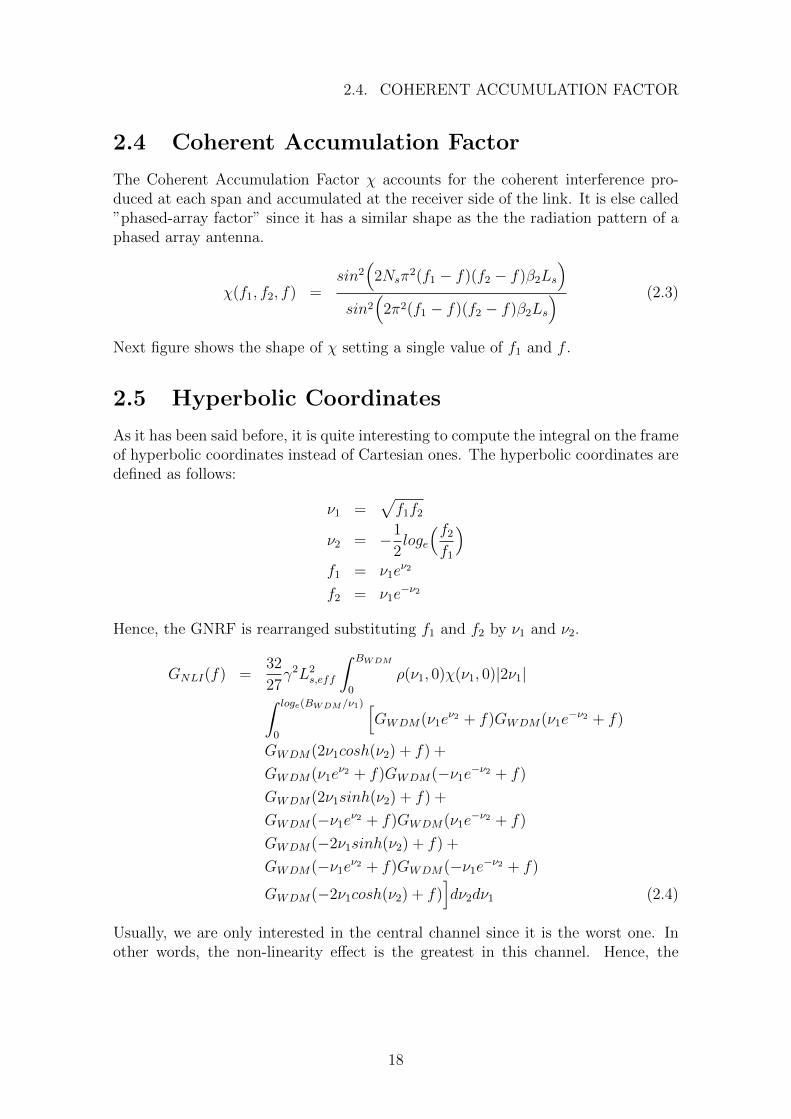
The Coherent Accumulation Factor χ accounts for the coherent interference pro-duced at each span and accumulated at the receiver side of the link. It is else called”phased-array factor” since it has a similar shape as the the radiation pattern of aphased array antenna.
χ(f1, f2, f) =sin2
⇣2Ns⇡2(f1 − f)(f2 − f)β2Ls
⌘
sin2⇣2⇡2(f1 − f)(f2 − f)β2Ls
⌘ (2.3)
Next figure shows the shape of χ setting a single value of f1 and f .
2.5 Hyperbolic Coordinates
As it has been said before, it is quite interesting to compute the integral on the frameof hyperbolic coordinates instead of Cartesian ones. The hyperbolic coordinates aredefined as follows:
⌫1 =p
f1f2
⌫2 = −1
2loge
⇣f2f1
⌘
f1 = ⌫1e⌫2
f2 = ⌫1e−⌫2
Hence, the GNRF is rearranged substituting f1 and f2 by ⌫1 and ⌫2.
GNLI(f) =32
27γ2L2
s,eff
Z BWDM
0
⇢(⌫1, 0)χ(⌫1, 0)|2⌫1|Z log
e
(BWDM
/⌫1)
0
hGWDM(⌫1e
⌫2 + f)GWDM(⌫1e−⌫2 + f)
GWDM(2⌫1cosh(⌫2) + f) +
GWDM(⌫1e⌫2 + f)GWDM(−⌫1e−⌫2 + f)
GWDM(2⌫1sinh(⌫2) + f) +
GWDM(−⌫1e⌫2 + f)GWDM(⌫1e−⌫2 + f)
GWDM(−2⌫1sinh(⌫2) + f) +
GWDM(−⌫1e⌫2 + f)GWDM(−⌫1e−⌫2 + f)
GWDM(−2⌫1cosh(⌫2) + f)id⌫2d⌫1 (2.4)
Usually, we are only interested in the central channel since it is the worst one. Inother words, the non-linearity e↵ect is the greatest in this channel. Hence, the
18

2.5. HYPERBOLIC COORDINATES
GNRF at f=0, GNLI(0), is:
GNLI(0) =64
27γ2NsL
2s,eff
Z BWDM
/2
0
⇢(⌫1, 0)χ(⌫1, 0)|2⌫1|Z log
e
(BWDM
/2⌫1)
0
hGWDM(⌫1e
⌫2)GWDM(⌫1e−⌫2)
hGWDM(2⌫1cosh(⌫2)) +GWDM(2⌫1sinh(⌫2))
id⌫2d⌫1 (2.5)
where:
⇢(⌫1, 0) =
(((((1− e−2↵L
sej4⇡2β2Ls
⌫21
2↵− j4⇡2β2⌫21
(((((
2
L−2eff (2.6)
χ(⌫1, 0) =sin2
⇣2Ns⇡2⌫21β2Ls
⌘
sin2⇣2⇡2⌫21β2Ls
⌘ (2.7)
The hyperbolic transformation shows that most of the contribution of ⇢ is concen-trated around ⌫1 = 0. Hence, the hyperbolic domain of integration can be clipped-o↵, so that the numerical solution is faster and the accuracy remains. Figure 2.2illustrates this fact:
Figure 2.2: Clipping o↵ the integration beyond -30 dB makes the integration domain75% smaller
On the other hand, the distance between two consecutive peaks of χ increases as⌫1 increases. Then, a lot of samples of ⌫1 are needed so that all peaks are taken intoaccount. Therefore, another advantage of setting a threshold is that a reasonable
19

2.6. GN-MODEL APPROXIMATED FORMULA
number of samples are enough to represent χ properly. Figure 2.3 depicts χ whenthe domain of ⌫1 is cut-o↵.
Figure 2.3: χ(⌫1, 0) and threshold equal to -30 dB
2.6 GN-Model Approximated Formula
The GNRF(f) allows to compute the non-linear PSD at any frequency, in otherwords, the channel under test can be tuned easily.However, an approximated formulacan be derivated so that it substitutes the integral for GNLI(0) (Appendix F andG of [12]). At the central frequency the integration area is symmetric with respectto f1 + f2 − f axis. Therefore, it is assumed to have a circular-like shape. Thisnew integration domain helps to solve the integral analytically, however, it over-estimates the non-linear PSD since the new domain is higher than the real domain.The closed-formula for the f=0 is:
GNLI ⇡ 8
27
γ2G3WDML2
eff
⇡β2Leff,a
asinh⇣⇡2
2β2Leff,aB
2ch[N
2ch]
B
ch
∆f
⌘(2.8)
The approximation works properly inside these boundaries:
1. β2 ≥ 4 [ps2
km]
2. Rs ≥ 28 [GBaud/s]
3. Bch
∆f≥ 0.25
4. Spanloss ≥ 7 [dB]
20

2.7. NLI ACCUMULATION
2.7 NLI Accumulation
This section shows some simulations that summarize how the evolution of NLI PSDchanges vs either number of channels or number of spans. First of all, the evolutionagainst the number of spans is analyzed. Function gnli(Ns) (2.9) considers theevolution of NLI PSD with respect to NLI PSD at central frequency after one span.
gnli(Ns) =Gnli(0, Ns)
Gnli(0, 1)(2.9)
The system under analysis consists on 21 channels at 32 GBaud/s. The optical fiberused was SMF, the roll-o↵ factor was 0.3 and di↵erent frequency spacing values werecompared. Figure 2.4 shows NLI PSD evolution for 50 GHz, 38.4 GHz, 32 GHz andincoherent accumulation. The smaller the frequency spacing, the more incoherentis the NLI accumulation, as reported on the figure below. The results are foundthrough numerical integration of GNRF (2.1). Although others roll-o↵ factors havebeen also analyzed for 50 GHz, 38.4 GHz and 32 GHz, no significant di↵erent resultshave been observed. The NLI accumulation against number of channel is studiedas well. To do so, function gnli(Nch) (2.10) is defined. The scenario under analysisis SMF,50 GHz spacing and 32 GBaud/s channels with 0.3 roll-o↵ factor. Functiongnli(Nch) is normalized to 95 channels (full C-Band).
gnli(Nch) =Gnli(0, Ns)
Gnli(0, 95)(2.10)
Figure 2.4: Red solid line 50 GHz frequency spacing, green solid line 38.4 GHz andyellow solid line 32 GHz
The evolution of NLI PSD grows following a logarithm law as the number ofchannels grows as well. The accumulation profile has been analyzed after one span,
21
2.7. NLI ACCUMULATION
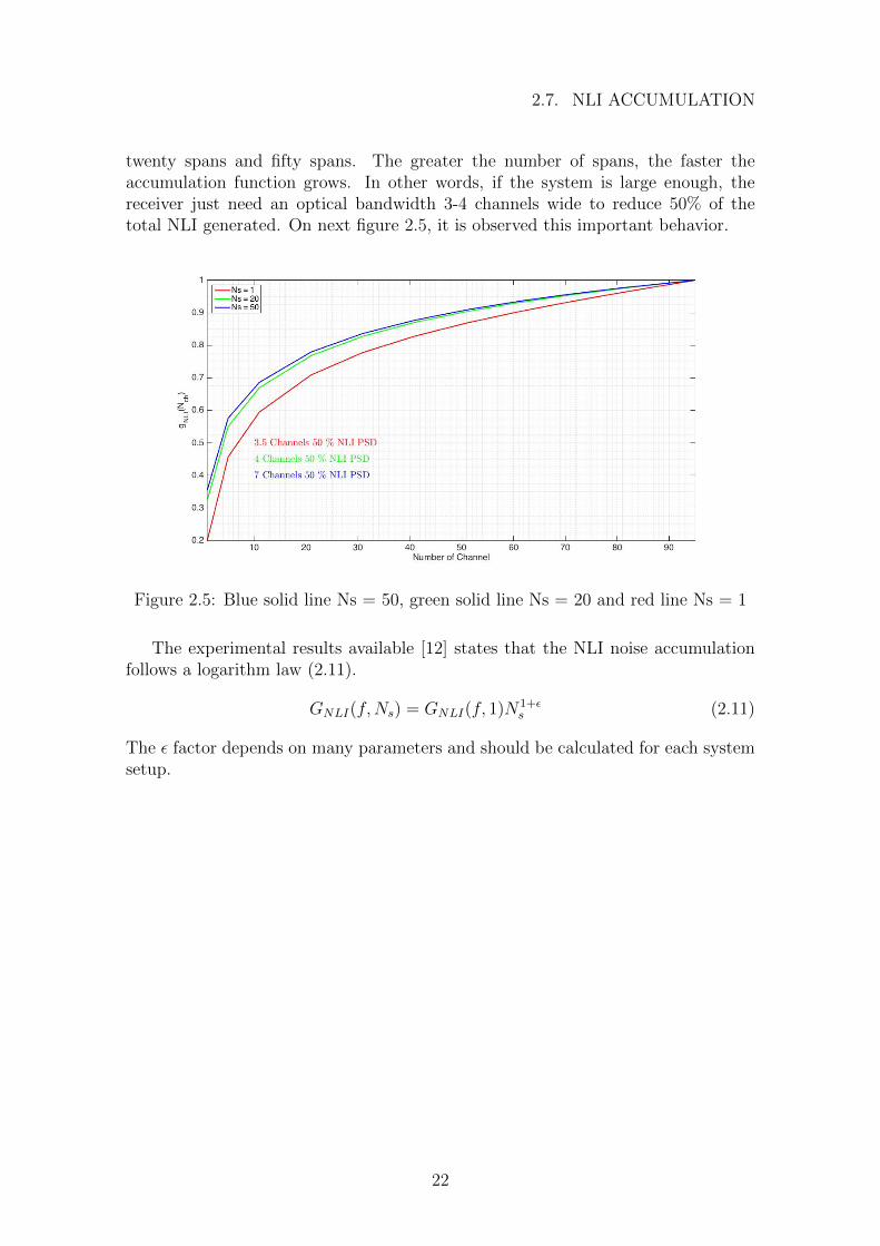
twenty spans and fifty spans. The greater the number of spans, the faster theaccumulation function grows. In other words, if the system is large enough, thereceiver just need an optical bandwidth 3-4 channels wide to reduce 50% of thetotal NLI generated. On next figure 2.5, it is observed this important behavior.
Figure 2.5: Blue solid line Ns = 50, green solid line Ns = 20 and red line Ns = 1
The experimental results available [12] states that the NLI noise accumulationfollows a logarithm law (2.11).
GNLI(f,Ns) = GNLI(f, 1)N1+✏s (2.11)
The ✏ factor depends on many parameters and should be calculated for each systemsetup.
22

Chapter 3
Generalized Gaussian Noise Model
In order to assess properly the performance of ultra-wideband optical networks (i.e.C+L systems), we need to considers spatial/frequency fiber parameters variations.To do so, GN-Model is remodeled assuming this dependence leading to the so-calledGeneralized Gaussian Model. All computations and assumptions are based on theGN-Model derivation [13]. However, some changes should be taken into account asloss/gain variation is not constant against frequency.
3.1 Generalized GN-Model Reference Formula
Here it is shown the mathematical derivation of the NLI PSD GNLI(f) when thepropagation and attenuation parameter depended on frequency, β(f)and↵(f). Then,the Generalized Gaussian Noise Model (GGN-Model) Reference Formula is depicted(3.18). This formula was derived on [1]. On this case, not only frequency variation,but also spatial/frequency variation of loss/gain is analyzed. The main di↵erenceis that, on the mathematical derivation shown below, the spatial integral is solvedas ↵(f) and β(f) does not change with z. However, on GGN-Model this integralcannot be solved. Following [13], the model is re-cast starting from the NLSE.
@
@zE(z, f) = [g(z, f)− jβ(f)]E(z, f) +QNLI(z, f) (3.1)
where:
1. g(z, f): Gain profile
2. β(f):Propagation constant
3. E(z, f) Electrical field
4. QNLI Kerr E↵ect term
Notice that when lumped-amplification is considered, g(z, f) = −↵(f). Then, weintroduce it into (3.1).
@
@zE(z, f) = [−↵(f)− jβ(f)]E(z, f) +QNLI(z, f) (3.2)
23
3.1. GENERALIZED GN-MODEL REFERENCE FORMULA
Where,
QNLI(z, f) = −jγE(z, f) ⇤ E⇤(z,−f) ⇤ E(z, f)
Since QNLI(z, f) depends on E(z,f) the equation can not be solved applying dif-ferential equation theory. We analyze the nature of QNLI(z, f) at the input of thefiber.
QNLI(0, f) = −jγE(0, f) ⇤ E⇤(0,−f) ⇤ E(0, f)
= −jγ
Z 1
−1E(0, f1)E
⇤(0,−(f − f1))df1 ⇤ E(0, f)
= −jγ
ZZ 1
−1E(0, f1)E
⇤(0, f1 − f2)E(0, f − f2)df1df2
(3.3)
Recall that the model defines the field as follows:
E(f) =pfoGTX(f)
1X
n=−1⇠nδ(f − nfo) (3.4)
We introduce (3.4) into QNLI(0, f) definition
QNLI(0, f) = −jγ
ZZ 1
−1
pfoGTX(f1)
1X
n=−1⇠nδ(f1 − nfo)
pfoGTX(f1 − f2)
1X
k=−1
⇠⇤kδ(f1 − f2 − kfo)
pfoGTX(f − f2)
1X
m=−1⇠mδ(f − f2 −mfo)
= −jγ1X
n=−1
1X
k=−1
1X
m=−1
pfo
3pGTX(nfo)GTX(kfo)GTX(mfo)
⇠n⇠⇤k⇠mδ(f1 − nfo)δ(f1 − f2 − kfo)δ(f − f2 −mfo)
= −jγ1X
n=−1
1X
k=−1
1X
m=−1
pfo
3pGTX(nfo)GTX(kfo)GTX(mfo)
⇠n⇠⇤k⇠mδ(−f2 − (k − n)fo)δ(f − f2 −mfo)
= −jγ1X
n=−1
1X
k=−1
1X
m=−1
pfo
3pGTX(nfo)GTX(kfo)GTX(mfo)
⇠n⇠⇤k⇠mδ(f − (n− k +m)fo)
We define the set Ai as the tuple (n,k,m) such that n-k+m=i Furthermore, thesubset Xi such that n-k+m=i and n=k or m=k. Therefore, Ai = Ai +Xi.
QNLI(0, f) = −jγfo3/21X
i=−1
δ(f − ifo)X
n,k,m2Ai
⇠n⇠⇤k⇠m
pGTX(nfo)GTX(kfo)GTX(mfo)
24

3.1. GENERALIZED GN-MODEL REFERENCE FORMULA
QNLI(0, f) = QNLI,Ai
(0, f) +QNLI,Xi
(0, f)
QNLI,Ai
(0, f) = −jγfo3/21X
i=−1
δ(f − ifo)X
n,k,m2Ai
⇠n⇠⇤k⇠m
pGTX(nfo)GTX(kfo)GTX(mfo)
QNLI,Xi
(0, f) = −jγfo3/21X
i=−1
δ(f − ifo)X
n,k,m2Xi
⇠n⇠⇤k⇠m
pGTX(nfo)GTX(kfo)GTX(mfo)
We analyze the subset Xi:
1. n-k+m=i and n=k ! n-n+m=i ! m=i
2. n-k+m=i and m=k ! n-m+m=i ! n=i
QNLI,Xi
(0, f) = −jγfo3/21X
i=−1
δ(f − ifo)
⇣X
k
X
k
X
i
⇠k⇠⇤k⇠i
pGTX(kfo)GTX(kfo)GTX(ifo)
+X
i
X
k
X
k
⇠i⇠⇤k⇠k
pGTX(ifo)GTX(kfo)GTX(kfo)
⌘
= −jγfo3/21X
i=−1
δ(f − ifo)
⇣2X
k
X
i
|⇠k|2⇠iGTX(kfo)pGTX(ifo)
⌘(3.5)
The power of a single realization of the random process is PE = fo1P
n=−1GTX(nfo)|⇠n|2
and it is also demonstrated that PE = PTX . We rearrange the expression:
QNLI,Xi
(0, f) = −j2γPTX
pfo
1X
i=−1
δ(f − ifo)pGTX(ifo)
= −j2γPTXE(0, f) (3.6)
We assume that this expression is still valid for any value of z.
QNLI,Xi
(z, f) = −j2γPTXe−2↵(f)
pfo
1X
i=−1
δ(f − ifo)pGTX(ifo)
Recall that:
E(f) =pfoGTX(f)
1X
n=−1⇠nδ(f − nfo)
25

3.1. GENERALIZED GN-MODEL REFERENCE FORMULA
Then,
QNLI(z, f) = −j2γPTXe−2↵(f)zE(f) +QNLI,A
i
Therefore, the NLSE becomes:
@
@zE(z, f) = [−↵(f)− jβ(f)− j2γPTXe
−2↵(f)z]E(z, f) +QNLI,Ai
(z, f)
(3.7)
Now, the model makes an assumption that allows to obtain a closed solution ofthe Eq. QNLI,A
i
(z, f) is considered independent from E(z, f). In other words, thenon-linearity interference is generated from a di↵erent source. Recalling the theoryfor first order linear di↵erential equation:
dy
dx+ p(x)y = q(x) (3.8)
The solution is:
y(x) = e−Rx
x0p(s)ds
hy0 +
Z x
x0
q(s)eRs
x0p(t)dtds
i(3.9)
Where:
y0 = y(0) ; x0 ! x = 0
Now we rearrange (3.7) to compare with (3.8).
@
@zE(z, f) + [↵(f) + jβ(f) + j2γPTXe
−2↵(f)z]E(z, f) = QNLI,Ai
(z, f)
We define function Γ(z, f) as:
Γ(z, f) = −Z z
0
[↵(f) + jβ(f) + j2γPTXe−2↵(f)z0 ]dz0
= −↵(f)z − jβ(f)z − j2γPTXzeff (z, f)
Where the e↵ective length varies with both frequency and length as it is defined:
zeff (z, f) =1− e−2↵(f)z
2↵(f)(3.10)
E(z, f) = eΓ(z,f)hE(0, f) +
Z z
0
QNLI,Ai
(z0, f)e−Γ(z0,f)dz0i
E(z, f) ⇡ ELIN(z, f) + ENLI(z, f)
26
3.1. GENERALIZED GN-MODEL REFERENCE FORMULA
ELIN(z, f) = eΓ(z,f)E(0, f)
ENLI = eΓ(z,f)Z z
0
QNLI,Ai
(z0, f)e−Γ(z0,f)dz0
The model considers the non-linearity noise-like signal as perturbation. In otherwords, it is much lower that the transmitted signal. Then, E(z, f) ⇡ ELIN(z, f)Therefore,
QNLI(z, f) ⇡ −jγELIN(z, f) ⇤ E⇤LIN(z,−f) ⇤ ELIN(z, f)
ELIN(z, f) = eΓ(z,f)E(0, f)
QNLI(z, f) ⇡ −jγh Z 1
−1eΓ(z,f1)E(0, f1)e
Γ⇤(z,f1−f)E⇤(0, f1 − f)df1i⇤ ELIN(z, f)
QNLI(z, f) ⇡ −jγh Z 1
−1e[−jβ(f1)z−↵(f1)z−j2γP
TX
zeff
(z,f1)]
E(0, f1)e[jβ(f1−f)z−↵(f1−f)z+j2γP
TX
zeff
(z,f1−f)]E⇤(0, f1 − f)df1i⇤ ELIN(z, f)
= −jγh ZZ 1
−1e[−jβ(f1)z−↵(f1)z−j2γP
TX
zeff
(z,f1)]
E(0, f1)e[jβ(f1−f2)z−↵(f1−f2)z+j2γP
TX
zeff
(z,f1−f2)]E⇤(0, f1 − f2)
e−jβ(f−f2)z−↵(f−f2)z−j2γPTX
zeff
(z,f−f2)E(0, f − f2)df1df2i
(3.11)
We define a function A(z, f1, f2, f)
A(z, f1, f2, f) = −j(β(f1)− β(f1 − f2) + β(f − f2))z
−(↵(f1) + ↵(f1 − f2) + ↵(f − f2))z
−j2γPTX(zeff (z, f1)− zeff (z, f1 − f2) + zeff (z, f − f2))
QNLI(z, f) ⇡ −jγ
ZZ 1
−1eA(z,f1,f2,f)E(0, f1)E
⇤(0, f1 − f2)E(0, f − f2)df1df2
Introducing (3.4) into previous expression:
QNLI(z, f) ⇡ −jγ
ZZ 1
−1eA(z,f1,f2,f)f 3/2
o
pGTX(f1)GTX(f1 − f2)GTX(f − f2)
X
n
X
k
X
m
⇠n⇠⇤k⇠mδ(f1 − nfo)δ(f1 − f2 − kfo)δ(f − f2 −mfo)df1df2
27

3.1. GENERALIZED GN-MODEL REFERENCE FORMULA
Integral solution is straightforward.
QNLI(z, f) ⇡ −jγf 3/2o
X
n
X
k
X
m
⇠n⇠⇤k⇠me
A(z,nfo
,kfo
,mfo
)
pGTX(nfo)GTX(kfo)GTX(mfo)δ(f − [n− k +m]fo)
Recalling that the set Ai is composed of n-k+m=i and Ai is that set such thatAi = Ai −Xi
QNLI,Ai
(z, f) ⇡ −jγf 3/2o
X
i
δ(f − ifo)X
n,k,m2Ai
⇠n⇠⇤k⇠me
A(z,nfo
,kfo
,mfo
)
pGTX(nfo)GTX(kfo)GTX(mfo) (3.12)
Now we focus on ENLI(z, f) so that we can compute the PSD of the non-linearity.
ENLI(z, f) = eΓ(z,f)Z z
0
QNLI,Ai
(z0, f)e−Γ(z0,f)dz0 (3.13)
(3.12) is introduced into (3.13):
ENLI = −jγf 3/2o e−jβ(f)ze−↵(f)ze−j2γP
TX
zeff
(z,f)
X
i
δ(f − ifo)X
n,k,m2Ai
pGTX(nfo)GTX(kfo)GTX(mfo)
Z z
0
ejβ(f)z0e↵(f)z
0ej2γPTX
zeff
(z0,f)eA(z0,f1,f2,f)dz0 (3.14)
The integral is quite tedious because of zeff (z, f) changes with frequency since itdepends on ↵(f). Then, it is more convenient to use an equivalent expression of Eq(26) where we do not split the set Ai into Ai and Xi. The equivalent expression ofthe non-linear field is:
ENLI(z, f) ⇡X
i
δ(f − ifo)h− jγf 3/2
o e
h−jβ(f)−↵(f)
iz
X
m,n,k2Ai
⇠n⇠⇤k⇠m
pGTX(nfo)GTX(kfo)GTX(mfo)
Z z
0
ej∆βz0e∆↵z0dz0i
Where,
∆β = β([n− k +m]fo)− β(nfo) + β(kfo)− β(mfo)
∆↵ = ↵([n− k +m]fo)− ↵(nfo)− ↵(kfo)− ↵(mfo)
The expression is the same, but it is quite easier to integrate. Previously, the factorzeff appeared on Γ(z, f) and only the subset Ai a↵ected ENLI since the subset
28

3.1. GENERALIZED GN-MODEL REFERENCE FORMULA
Xi only added a term proportional to E(z, f). This division is a good choice forGN-Model because it considers constant parameters, so that zeff is constant for allfrequency components and it is canceled inside QNLI,A
i
, not increasing the integralcomplexity. We solve the integral,
Z z
0
e(j∆β+∆↵)z0dz0 =1
j∆β +∆↵
Z z
0
(j∆β +∆↵)e(j∆β+∆↵)z0dz0
=1
j∆β +∆↵
he(j∆β+∆↵)z − 1
i
=1− e(j∆β+∆↵)z
−∆↵− j∆β
ENLI(z, f) =X
i
µiδ(f − ifo) (3.15)
The NLI disturbance is a set of deltas. The power spectral density of a given instanceof such process would be:
⇥ENLI
(f) =X
i
|µi|2δ(f − ifo) (3.16)
We use the statistical expectation operator to compute the average PSD.
GENLI
(f) = E{⇥ENLI
(f)}=
X
i
E{|µi|2}δ(f − ifo)
We focus on |µi|2 = µiµ⇤i
|µi|2 =h− jγf 3/2
o e[−jβ(f)−↵(f)]zX
n,k,m2Ai
⇠n⇠⇤k⇠m
pGTX(nfo)GTX(kfo)GTX(mfo)
1− e(j∆β+∆↵)z
−∆↵− j∆β
ihjγf 3/2
o e[jβ(f)−↵(f)]z
X
n0,k0,m02Ai
⇠⇤n⇠k⇠⇤m
pGTX(n0fo)GTX(k0fo)GTX(m0fo)
1− e(−j∆β+∆↵)z
−∆↵ + j∆β
i
|µi|2 = γ2f 3o e
−2↵(f)zX
n,k,m2Ai
X
n0,k0,m02Ai
⇠n⇠0⇤n ⇠
⇤k⇠
0k⇠m⇠
0⇤m
pGTX(nfo)GTX(kfo)GTX(mfo)
pGTX(n0fo)GTX(k0fo)GTX(m0fo)
(((1− e(j∆β+∆↵)z
−∆↵− j∆β
(((2
29

3.1. GENERALIZED GN-MODEL REFERENCE FORMULA
E{|µi|2} = γ2f 3o e
−2↵(f)zX
n,k,m2Ai
X
n0,k0,m02Ai
E{⇠n⇠0⇤n ⇠⇤k⇠0k⇠m⇠0⇤m}
pGTX(nfo)GTX(kfo)GTX(mfo)
pGTX(n0fo)GTX(k0fo)GTX(m0fo)
(((1− e(j∆β+∆↵)z
−∆↵− j∆β
(((2
(3.17)
It is demonstrated [13] that:
E{⇠n⇠0⇤n ⇠⇤k⇠0k⇠m⇠0⇤m} = E{|⇠n|2}E{|⇠k|2}E{|⇠m|2} = 1
Following the procedure in [13], an approximation of (3.17) is given:
E{|µi|2} ⇡ 2γ2f 3o e
−2↵(f)zX
n
X
m
GTX(nfo)GTX(mfo)GTX([n+m− i]fo)
(((1− e{↵(ifo)−↵(nf
o
)−↵([n+m−i]fo
)−↵(mfo
)}zej{β(ifo)−β(nfo
)+β([n+m−i]fo
)−β(mf0)}z
−↵(ifo) + ↵(nfo) + ↵([n+m− i]fo) + ↵(mfo)− j{β(ifo)− β(nfo) + β([n+m− i]fo)− β(mf0)}
(((2
Therefore, the PSD of the non-linearity interference for the Single Polarization case.
GENLI
(f) = 2γ2f 3o e
−2↵(f)zX
i
δ(f − ifo)X
n
X
m
GTX(nfo)GTX(mfo)GTX([n+m− i]fo)
(((1− e{↵(ifo)−↵(nf
o
)−↵([n+m−i]fo
)−↵(mfo
)}zej{β(ifo)−β(nfo
)+β([n+m−i]fo
)−β(mf0)}z
−↵(ifo) + ↵(nfo) + ↵([n+m− i]fo) + ↵(mfo)− j{β(ifo)− β(nfo) + β([n+m− i]fo)− β(mf0)}
(((2
The expansion for Dual-Polarization case is explained in [13].
GENLI
(f) =16
27γ2f 3
o e−2↵(f)z
X
i
δ(f − ifo)X
n
X
m
GTX(nfo)GTX(mfo)GTX([n+m− i]fo)
(((1− e{↵(ifo)−↵(nf
o
)−↵([n+m−i]fo
)−↵(mfo
)}zej{β(ifo)−β(nfo
)+β([n+m−i]fo
)−β(mf0)}z
−↵(ifo) + ↵(nfo) + ↵([n+m− i]fo) + ↵(mfo)− j{β(ifo)− β(nfo) + β([n+m− i]fo)− β(mf0)}
(((2
The transition to a frequency-continuous domain:
GENLI
(f) =16
27γ2e−2↵(f)z
1Z
−1
1Z
−1
GTX(f1)GTX(f2)GTX(f1 + f2 − f)
(((1− e{↵(f)−↵(f1)−↵(f1+f2−f)−↵(f2)}zej{β(f)−β(f1)+β(f1+f2−f)−β(f2)}z
−↵(f) + ↵(f1) + ↵(f1 + f2 − f) + ↵(f2)− j{β(f)− β(f1) + β(f1 + f2 − f)− β(f2)}
(((2
The GNRF of GGN-Model is depicted above [1].
GNLI(f) =16
27γ2⇢(z, f)2
1Z
−1
1Z
−1
GTX(f1)GTX(f2)GTX(f1 + f2 − f)
(((zZ
0
ej4⇡2(f1−f)(f2−f)β2⇣
⇢(⇣, f1)⇢(⇣, f3)⇢(⇣, f2)
⇢(⇣, f)d⇣
(((2
df1df2 (3.18)
30

3.2. FWM EFFICIENCY FACTOR
3.2 FWM Efficiency Factor
One of the di↵erence between GN-Model and GGN-Model is how the FWM Effi-ciency Factor is addressed. On the GN-Model, the spatial integral is easily solvedas the parameters remains constant along both space and frequency. However, itchanges when the parameters are considered variable. Next expression shows theFWM Efficiency factor for GGN-Model.
⇢(z, f1, f2, f) =(((
zZ
0
ej4⇡2(f1−f)(f2−f)β2⇣
⇢(⇣, f1)⇢(⇣, f3)⇢(⇣, f2)
⇢(⇣, f)d⇣
(((2
(3.19)
Recall that this factor for GN-Model follows the expression depicted in 2.2.
⇢(f1, f2, f) =
(((((1− e−2↵L
sej4⇡2β2Ls
(f1−f)(f2−f)
2↵− j4⇡2β2(f1 − f)(f2 − f)
(((((
2
L−2eff
Clearly, the function shown above does not depend on z, as the integral was solvedanalytically. On the other hand, the integral 3.19 should be solved numerically.First of all, the function to be integrated is analyzed. It is a complex exponentialdamped by the field profile of all pumps frequencies. The factor (f1 − f)(f2 − f)determines the slope of the complex exponential. In other words, the frequency of thesinusoidal functions derived from the complex exponential. This features determinesthe number of samples on z needed to solve the integral properly. Furthermore, thisis a critical issue, as it determines the simulation time. For example, when f1 andf2 are close to the frequency under analysis f , then the sinusoidal functions are slow(Figure 3.1). Therefore, few nS are needed. However, the minimum nS increases asboth f1 and f2 move away from f (Figure 3.2).
Figure 3.1: Blue solid line real part of the complex exponential and red dashed linesfield profile of pumps frequencies, when (f1 − f)(f2 − f) is low.
31

3.2. FWM EFFICIENCY FACTOR
Figure 3.2: Blue solid line real part of the complex exponential and red dashed linesfield profile of pumps frequencies, when (f1 − f)(f2 − f) is high.
The reader can wonder what is the consequence of not determine properly thenumber of samples. The answer is clearly that the model provides an over/underestimate. Function IGGN
2 (f1, f) is defined as:
IGGN2 (f1, f) = GTX(f1)
Bw
/2Z
−Bw
/2
GTX(f2)GTX(f1 + f2 − f)
(((zZ
0
ej4⇡2(f1−f)(f2−f)β2⇣
⇢(⇣, f1)⇢(⇣, f)⇢(⇣, f2)
⇢(⇣, f3)d⇣
(((2
df2 (3.20)
Function IGN2 (f1, f) is defined as:
IGN2 (f1, f) = GTX(f1)
Bw
/2Z
−Bw
/2
GTX(f2)GTX(f1 + f2 − f)
(((((1− e−2↵L
sej4⇡2β2Ls
(f1−f)(f2−f)
2↵− j4⇡2β2(f1 − f)(f2 − f)
(((((
2
df2 (3.21)
Later on, function I2(f1, f) is integrated with respect to f1. Both functions shouldmatch for the case of constant parameters if only if nS is properly set. Figures 3.3show the misleading result when nS is not correct.
32

3.2. FWM EFFICIENCY FACTOR
Figure 3.3: Blue solid line represents IGN2 and red dashed line represents IGGN
2
At first sight, it seems that the mismatching does not a↵ect the results so muchas it is 20 dB lower than the main lobe. However, it does as the number of channelsincreases. To sum up, it can be state that optimal number of sample is variable anddepends on what pumps frequency are being analyzing.
33

Chapter 4
Metric to assess Quality ofTransmission (QoT)
4.1 Metric definition and GN-Model implications
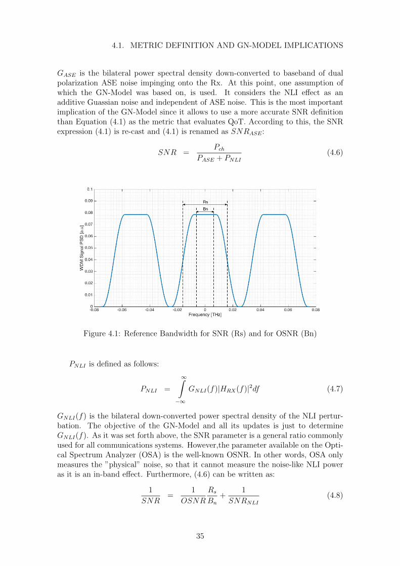
From the physical layer point of view, the most common metric to evaluate the QoTis the Signal-to-Noise Ratio (SNR) (4.1). In optics, however, the widely used pa-rameter is the so called Optical-Signal-to-Noise Ratio (OSNR) (4.2). The di↵erenceis the reference bandwidth (Figure 4.1). In optical communications the referencebandwidth to measure the noise is typically around 12.48 GHz (0.1 nm). Thus, (4.1)is obtained after the post-procesing stage and (4.2) is the ”physical” value obtainedby the Optical Spectrum Analyzer. Next expressions are taken from [14].
SNR =Pch
PASE
(4.1)
OSNR =Rs
BnSNR (4.2)
Furthermore, under Linear Propagation and Gaussian Noise scenario the relationbetween Bit Error Rate (BER) and SNR is [14]:
BER =1
2erfc
⇣pSNR/2
⌘(4.3)
Pch is the received channel power and PASE is the noise power produced by EDFAamplifiers.
Pch = PRXR−1s
1Z
−1
|HRX(f)|2df (4.4)
PASE =
1Z
−1
GASE|HRX(f)|2df (4.5)
34
4.1. METRIC DEFINITION AND GN-MODEL IMPLICATIONS
GASE is the bilateral power spectral density down-converted to baseband of dualpolarization ASE noise impinging onto the Rx. At this point, one assumption ofwhich the GN-Model was based on, is used. It considers the NLI e↵ect as anadditive Guassian noise and independent of ASE noise. This is the most importantimplication of the GN-Model since it allows to use a more accurate SNR definitionthan Equation (4.1) as the metric that evaluates QoT. According to this, the SNRexpression (4.1) is re-cast and (4.1) is renamed as SNRASE:
SNR =Pch
PASE + PNLI
(4.6)
Figure 4.1: Reference Bandwidth for SNR (Rs) and for OSNR (Bn)
PNLI is defined as follows:
PNLI =
1Z
−1
GNLI(f)|HRX(f)|2df (4.7)
GNLI(f) is the bilateral down-converted power spectral density of the NLI pertur-bation. The objective of the GN-Model and all its updates is just to determineGNLI(f). As it was set forth above, the SNR parameter is a general ratio commonlyused for all communications systems. However,the parameter available on the Opti-cal Spectrum Analyzer (OSA) is the well-known OSNR. In other words, OSA onlymeasures the ”physical” noise, so that it cannot measure the noise-like NLI poweras it is an in-band e↵ect. Furthermore, (4.6) can be written as:
1
SNR=
1
OSNR
Rs
Bn
+1
SNRNLI
(4.8)
35
4.2. MAXIMUM LENGTH
Where SNRNLI is defined as :
SNRNLI =Pch
PNLI
(4.9)
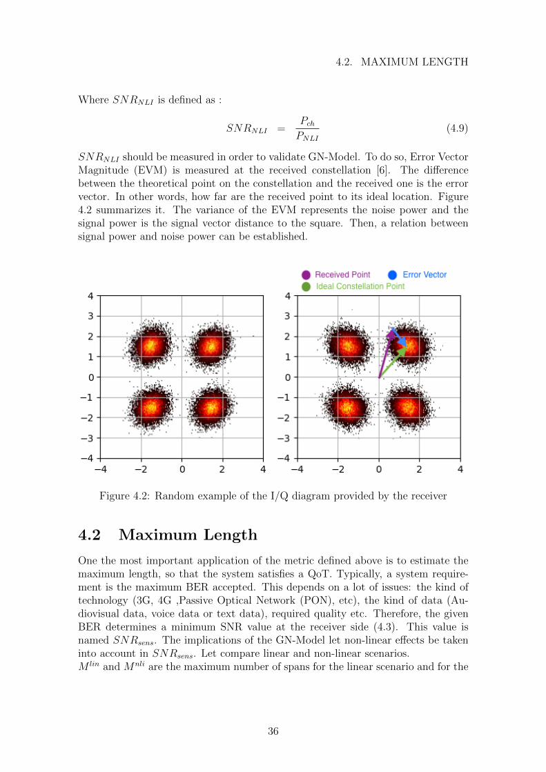
SNRNLI should be measured in order to validate GN-Model. To do so, Error VectorMagnitude (EVM) is measured at the received constellation [6]. The di↵erencebetween the theoretical point on the constellation and the received one is the errorvector. In other words, how far are the received point to its ideal location. Figure4.2 summarizes it. The variance of the EVM represents the noise power and thesignal power is the signal vector distance to the square. Then, a relation betweensignal power and noise power can be established.
Figure 4.2: Random example of the I/Q diagram provided by the receiver
4.2 Maximum Length
One the most important application of the metric defined above is to estimate themaximum length, so that the system satisfies a QoT. Typically, a system require-ment is the maximum BER accepted. This depends on a lot of issues: the kind oftechnology (3G, 4G ,Passive Optical Network (PON), etc), the kind of data (Au-diovisual data, voice data or text data), required quality etc. Therefore, the givenBER determines a minimum SNR value at the receiver side (4.3). This value isnamed SNRsens. The implications of the GN-Model let non-linear e↵ects be takeninto account in SNRsens. Let compare linear and non-linear scenarios.M lin and Mnli are the maximum number of spans for the linear scenario and for the
36
4.2. MAXIMUM LENGTH
non-linear one, respectively.
SNRsens =Pch
M linPase
M lin =1
SNRsens
Pch
Pase
(4.10)
SNRsens is in linear scale, Pch is the input channel power and Pase is the noise powerinduced by the amplifiers. Note that Pase does not depend on Pch. Therefore, themaximum length is infinite since M lin grows as Pch does. In other words, M lin is alinear function of Pch. On the other hand, for the non-linear scenario case the SNRdefinition changes as explained on previous section (4.6).
SNRsens =Pch
MnliPase +MnliPnli
SNRsens =Pch
MnliPase +Mnli⌘(1)Pch
Mnli =1
SNRsens
Pch
Pase + ⌘(1)P 3ch
(4.11)
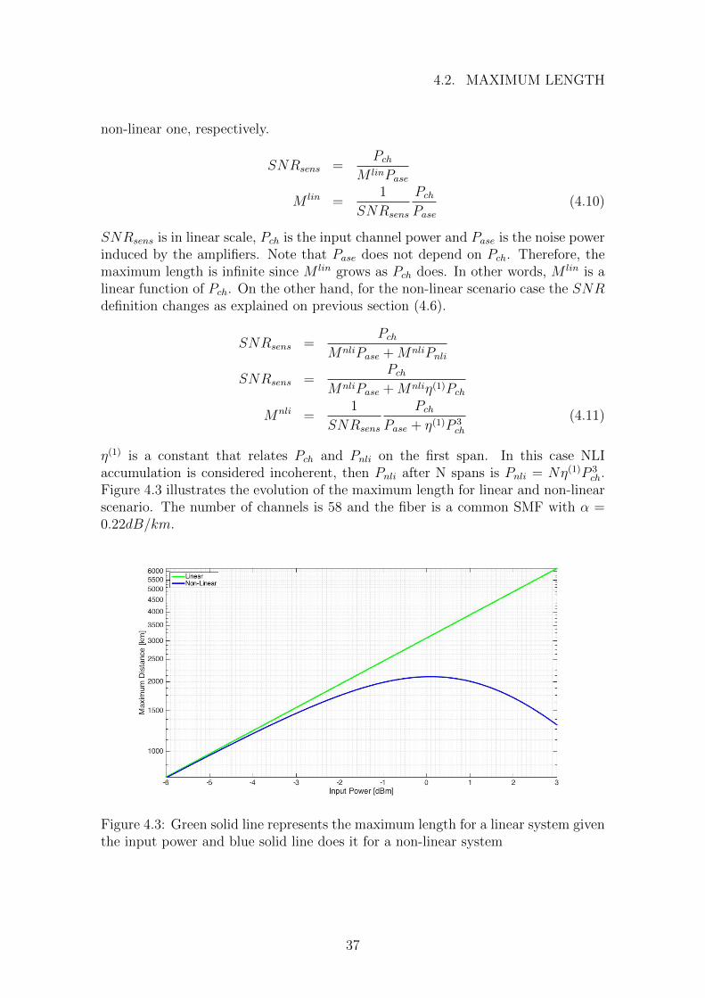
⌘(1) is a constant that relates Pch and Pnli on the first span. In this case NLIaccumulation is considered incoherent, then Pnli after N spans is Pnli = N⌘(1)P 3
ch.Figure 4.3 illustrates the evolution of the maximum length for linear and non-linearscenario. The number of channels is 58 and the fiber is a common SMF with ↵ =0.22dB/km.
Figure 4.3: Green solid line represents the maximum length for a linear system giventhe input power and blue solid line does it for a non-linear system
37

Chapter 5
Model implementation
Both models have been implemented in order to carry out simulations that allowto estimate the system performance evaluation. Thus, the developed tool is usefulto plan optical networks a↵ected by non-linear e↵ect. Moreover, the software toolimplmented on this Master Thesis is also flexible as di↵erent models can be chosendepending on the accuracy level desired. For instance, if only preliminary analysisof NLI e↵ect at central frequency is expected, it is highly recommendable to useGN-Model approximated formula (2.8) as the algorithm is executed very fast. If amore detailed analysis is expected and the number of channels is not large enough sothat the fiber parameters change a lot (in C-Band attenuation frequency dependenceis soft) GN-Model (2.1) can be used. On the other hand, if we are dealing with aultra-wide-band optical system (involving C+L Bands) GGN-Model is the propermodel to estimate NLI at any frequency. The code has been divided as follows:fiber parameters are defined on an independent Matlab file, system parameters aredefined on another independent Matlab file and the GN-Model approximated for-mula (2.8), the GN-Model (2.1) and the GGN-Model (3.18) are also developed onan independent Matlab file each one.
5.1 Code Structure
On this section, the code structure is deeply explained so that others can use thetool. As it is said above, the main three parts are: fiber parameters definition,system parameters definition and model implementation.
5.1.1 Fiber Parameters
The fiber parameters are defined on the Matlab file named as ”fiberParam.m”. Thisfile is an ad-hoc defined function. It uses two facilities available on the Matlabenvironment: struct data type and switch-case expression. The struct data typeallows to group related parameters using data containers called fields. For ourpurpose, this way to organize the code is significantly useful since all fiber parametersare grouped together and all of them are related to a type of fiber. On the other
38
5.1. CODE STRUCTURE
hand, the switch-case expression allows to select a fiber and hence all its parameters.The function input and output variables are listed above:
• Input
– fiberType String Data Type. Used by switch-case structure to selectthe fiber.
• Output
– fiberParams Struct Data Type. It contains fiber parameters.
The fields inside fiberParams struct are listed and explained below:
• GVD Group Velocity Dispersion [ps2
km].
• alpha Attenuation Coefficient. Electric field definition [ 1km
].
• gamma Kerr E↵ect Coefficient. [W−1km−1].
The procedure to define a new type of fiber is basically to open ”fiberParam.m”,to define a new case with the fiber type name and to fill its fields with the fiberparameters values. For example, next figure shows a SMF with D = to be filled,alpha = to be filled and gamma = to be filled.
5.1.2 System-Signal Parameters
Both signals and system parameters are defined in the same Matlab file named as”systemParams.m”. This file is an ad-hoc defined function. It follows the samestrategy as the one used for ”fiberParam.m”. The input and the variables of thefunction are listed below:
• Input
– delta f Double Data Type. Spacing frequency in [THz].
– article String Data Type. System name reference.
– nCh Double Data Type. Number of Channels.
– power Double Data Type. Channel Power in [dBm].
• Output
– signal Struct Data Type. It contains signal parameters.
– sys Struct Data Type. It contains system parameters.
The fields inside both signal and sys structs are listed:
• signal
– roll o↵ Double Data Type. Roll-o↵ factor.
– Rs Double Data Type. Symbol Rate in [GBauds].
– power Double Data Type. Channel Power in [dBm] .
– BwCh Double Data Type. Channel Bandwidth in [THz].
39

5.1. CODE STRUCTURE
• sys
– Flin Double Data Type. Figure Noise in linear scale.
– GLin Double Data Type. EDFA Gain in linear scale.
– Ls Double Data Type. Span length in [km].
– nCh Double Data Type. Number of Channels.
– delta f Double Data Type. Spacing frequency in [THz].
– Bw Double Data Type. Total Bandwidth in [THz].
– Ns Double Data Type. Number of Spans.
– fCh Double Data Type. Central frequency of each channel in [THz].
– fo Double Data Type. Central frequency in [THz]
The procedure to define a new set of parameters in order to simulate a systemis basically to open the file ”systemParams.m”. Next figure a case of a systemdefinition.
5.1.3 GN-Model Approximated Formula
The file name as ”GNLI aprox.m” computes the GN-Model based on the approxi-mated formula defined on (2.8). The input and output variables are listed below:
• Input
– fiberParams Struct Data Type. It contains fiber parameters.
– signal Struct Data Type. It contains signal parameters.
– sys Struct Data Type. It contains system parameters.
• Output
– gnli Double Data Type. NLI PSD in [ WHz
].
5.1.4 GN-Model Cartesian Coordinates
The file named as ”GNLI f.m” computes the GN-Model through numerical integra-tion (2.1). The integral is solved on Cartesian coordinates (f1, f2). The input andoutput variables are listed below:
• Input
– fiberParams Struct Data Type. It contains fiber parameters.
– signal Struct Data Type. It contains signal parameters.
– sys Struct Data Type. It contains system parameters.
– f Double Data Type. Frequency under analysis on base-band in [THz].
– gtx Double Array Data Type. WDM-Signal PSD in [ WHz
].
40
5.1. CODE STRUCTURE
• Output
– GNLI Double Data Type. NLI PSD in [ WHz
].
5.1.5 GN-Model Hyperbolic Coordinates
The file named as ”GNLI f hyp.m” computes the GN-Model through numericalintegration (2.4). The integral is solved on Hyperbolic coordinates (⌫1, ⌫2). Theinput and output variables are listed below:
• Input
– fiberParams Struct Data Type. It contains fiber parameters.
– signal Struct Data Type. It contains signal parameters.
– sys Struct Data Type. It contains system parameters.
– f Double Data Type. Frequency under analysis on base-band in [THz].
– gtx Double Array Data Type. WDM-Signal PSD in [ WHz
].
• Output
– GNLI Double Data Type. NLI PSD in [ WHz
].
5.1.6 GN-Model Hyperbolic Coordinates for f=0
The file named as ”GNLI 0 hyp.m” computes the GN-Model through numericalintegration (2.5). The integral is solved on Hyperbolic coordinates (⌫1, ⌫2). Theinput and output variables are listed below:
• Input
– fiberParams Struct Data Type. It contains fiber parameters.
– signal Struct Data Type. It contains signal parameters.
– sys Struct Data Type. It contains system parameters.
• Output
– GNLI Double Data Type. NLI PSD in [ WHz
].
5.1.7 GGN-Model Matrix Solution
The file named as ”GGNLI f.m” computes the GGN-Model through numerical in-tegration (3.18).The Matrix Solution is explained on 5.2.2. The input and outputvariables are listed below:
• Input
– fiberParams Struct Data Type. It contains fiber parameters.
– signal Struct Data Type. It contains signal parameters.
41

5.1. CODE STRUCTURE
– sys Struct Data Type. It contains system parameters.
– f Double Data Type. Frequency under analysis on base-band in [THz].
– fibProf Double Matrix Type [nchxzetasamples]. Power Evolution Pro-file.
– sigPSD Double Array Data Type. WDM-Signal PSD in [ WHz
].
– zeta samples Double Type. Number of samples for z. It should be theminimum to solve the worst case.
• Output
– GGf Double Array Data Type. NLI PSD in [ WHz
].
5.1.8 GGN-Model Loop/Matrix Solution
The file named as ”GGNLI f 2.m” computes the GGN-Model through numericalintegration (3.18).This function is almost equal than the previous one. The loop/-Matrix solution refers to how the spatial integral of GGN-Model (3.18) is solved.The di↵erence with respect to Matrix Solution is just that f2 enters into a for loopinstead of being computed on one go. The input and output variables are listedbelow:
• Input
– fiberParams Struct Data Type. It contains fiber parameters.
– signal Struct Data Type. It contains signal parameters.
– sys Struct Data Type. It contains system parameters.
– f Double Data Type. Frequency under analysis on base-band in [THz].
– fibProf Double Matrix Type [nchxzetasamples]. Power Evolution Pro-file.
– sigPSD Double Array Data Type. WDM-Signal PSD in [ WHz
].
– zeta samples Double Type. Number of samples for z. It should be theminimum to solve the worst case.
• Output
– GGf Double Data Type. NLI PSD in [ WHz
].
5.1.9 GGN-Model Hybrid Solution
The file named as ”GGNLI f 3.m” computes the GGN-Model through numericalintegration (3.18). This function computes just the channel under test and its neigh-bors . The tails of (3.20) is filled by (3.21) The input and output variables are listedbelow:
42

5.2. CODE PERFORMANCE
• Input
– fiberParams Struct Data Type. It contains fiber parameters.
– signal Struct Data Type. It contains signal parameters.
– sys Struct Data Type. It contains system parameters.
– f Double Data Type. Frequency under analysis on base-band in [THz].
– fibProf Double Matrix Type [nchxzetasamples]. Power Evolution Pro-file.
– sigPSD Double Array Data Type. WDM-Signal PSD in [ WHz
].
– zeta samples Double Type. Number of samples for z. It should be theminimum to solve the worst case.
– I2 gn Double Array Data Type. Function (3.20)
– channel Double Type. Channel under analysis.
• Output
– GGf Double Data Type. NLI PSD in [ WHz
].
Figure 5.1 provides to the reader a general view of the code and how di↵erentfractions of it interact each other.
Figure 5.1: Code Architecture
5.2 Code performance
The main limitation of both the GN-Model and the GGN-Model is its computingtime. As the number of channels increases, then the total bandwidth grows as
43

5.2. CODE PERFORMANCE
well, more number of samples are required in order to solve properly the integral.Therefore, this limitation determine the maximum number of channels, that canbe simulated depending on the hardware resources. Besides all, this imperfectionbecomes more critical when GGN-Model is computed, as the spatial integral isintroduced to consider the spatial dependence as well. All this issues are brieflyanalyzed on this section.
5.2.1 Hyperbolic Coordinates vs Cartesian Coordinates
The hyperbolic reference system, derived on Appendix E (”Details of the derivationof the GNRF in hyperbolic Coordinates”) of [12], reduces significantly the com-puting time with respect to the one of the Cartesian Coordinates approach. Thecomputing time has been measured using the Matlab command called ”tic-toc”.A WDM system along SMF fiber has been simulated. The signals are 32 GBaud/sand 50 GHz frequency spaced. The number of channels is varied from 3 to 101channels. Both Cartesian based model and Hyperbolic Coordinates based one com-puting times have been measured through ”tic-toc” command as explained above.Figure 5.2 shows the evolution of the consuming time for both cases.
Figure 5.2: The graph shows the computing time of the GN-Model for di↵erentnumber of channels.Blue solid line represents Cartesian Coordinates approach andred solid line does Hyperbolic Coordinates one. Cartesian Coordinates approach isfaster than Hyperbolic Coordinates one until 10 channels. Beyond 10 channels isthe other way around.
The Hyperbolic Coordinates approach is slower until 10 channels, however it ismuch faster than the Cartesian Coordinates one. The reasons comes from the factthrough the Hyperbolic Coordinates approach many samples are avoided as most
44
5.2. CODE PERFORMANCE
of the NLI energy is accumulated as ⌫1 goes to zero, decreasing exponentially as ⌫1increases (Figure 2.2).
5.2.2 Generalized Gaussian Noise Model Matrix Solution
One of the critical issues of the GGN-Model implementation is how the integrals aresolved, specially, for ultra wide-band system. Thus, it is fundamental to implementit as optimal as possible. Matlab environment works much faster with vector-basedimplementations rather than with loop-based implementations. According to this,the model has been implemented as follows:
Recall the GNRF (3.18):
GNLI(z, f) =16
27γ2⇢(z, f)2
1Z
−1
1Z
−1
GTX(f1)GTX(f2)GTX(f1 + f2 − f)
(((zZ
0
ej4⇡2(f1−f)(f2−f)β2⇣
⇢(⇣, f1)⇢(⇣, f3)⇢(⇣, f2)
⇢(⇣, f)d⇣
(((2
df1df2
For the sake of clearness, the function is renamed.
G(f1, f2, f) = GTX(f1)GTX(f2)GTX(f1 + f2 − f) (5.1)
Z(f1, f2, f, ⇣) = ej4⇡2(f1−f)(f2−f)β2⇣
⇢(⇣, f1)⇢(⇣, f3)⇢(⇣, f2)
⇢(⇣, f)(5.2)
(5.1) and (5.2) are introduced into the GNRF (3.18).
GNLI(z, f) =16
27γ2⇢(z, f)2
1Z
−1
1Z
−1
G(f1, f2, f)
(((zZ
0
Z(f1, f2, f, ⇣)d⇣(((2
df1df2
The variable f is the frequency under analysis, then it is a single double value onthe code. f1 and f2 are double vectors spanning from −Bw/2 until Bw/2. ⇣ is alsoa double vector from 0 until Ls (Span Length) and z is the spatial position whereGNLI(z, f) is computed, it is usually at the end of the span (Ls). The integral aresolved as follows: A loop is built up. The loop length is equivalent to f1 one. Thus,on ith iteration f1 is set to a single value, i.e. f1 = f1(i).
G(f1(i), f2, f) = GTX(f1(i))GTX(f2)GTX(f1(i) + f2 − f) (5.3)
Z(f1(i), f2, f, ⇣) = ej4⇡2(f1(i)−f)(f2−f)β2⇣
⇢(⇣, f1(i))⇢(⇣, f3)⇢(⇣, f2)
⇢(⇣, f)(5.4)
45
5.2. CODE PERFORMANCE
At this point, a matrix can represents the integration function of ⇣-integral as thereare only two variables (f2 and ⇣). In other words, Z(f1, f2, f, ⇣) is implementedas a matrix where each column represents one sample of ⇣ and all samples of f2,meanwhile, each row represents one sample of f2 and all samples of ⇣. Thus, Z isthe integration function on a matrix-like shape.
Z =
2
6664
z11 z12 z13 . . . z1nz21 z22 z23 . . . z2n...
......
. . ....
zm1 zm2 zm3 . . . zmn
3
7775(5.5)
f2 2h− Bw
2,Bw
2
i
⇣ 2h0, Ls
i
For instance the element z13 represents the value for f2(1) and ⇣(3). Later on, theintegral is solved numerically row by row, as the variable to be integrated is ⇣.However, as the number of channels grows, the number of samples for f2 grows aswell as for ⇣ (see Figures 3.1 and 3.2). At a certain number of channels, the matrixdimensions become so huge that our hardware resources are not able to manage thematrix. To cope with this, another method to solve the triple integral has beendesigned : Loop/Matrix Solution 5.2.3. The numerical solution of the integral ofthe matrix gives a vector as a result. This vector is named I2 and represents nextfunction:
I(f2, f1(i), f) =(((
zZ
0
Z(f1, f2, f, ⇣)d⇣(((2
(5.6)
The I2 length is equal to f2 one. Then, f2-integral is solved numerically. The resultsis stored on vector I1. The length of I1 is equal to I1 one. At the end, of the loopvector I1 has been filled up for all samples of f1.
5.2.3 Generalized Gaussian Noise Model Loop/Matrix So-lution
As it has been set forth above, for ultra wide-band system the matrix solutionbecomes una↵ordable for the computing capacity of common hardware resources.Then, loop/matrix solution has been designed. On this approach a new loop isadded. The length of the new loop is equal to the number of channels. At eachiteration the matrix solution is applied. However, number of rows is reduced as f2interval is not f2 2 [−Bw/2, Bw/2] but f2 2 [−BwCh/2, BwCh/2]. Adding a new
46

5.2. CODE PERFORMANCE
loop is less efficient, but on the other hand matrix dimensions are smaller.
Z =
2
6664
z11 z12 z13 . . . z1nz21 z22 z23 . . . z2n...
......
. . ....
zk1 zm2 zm3 . . . zkn
3
7775(5.7)
f2 2h− BwCh
2,BwCh
2
i
⇣ 2h0, Ls
i
Eventually, if our hardware resources does not allow us to manage matrices so big,the second approach is required, even though the computation is slower.
5.2.4 Generalized Gaussian Noise Model Hybrid Solution
On section 3.2 the FWM Efficiency Factor is addressed and how it a↵ects the com-puting time. First of all, a fixed number of samples was considered. In this case,the worst case should be analyzed. The reason is that the integral should be solvedproperly when (f1 − f)(f2 − f) is both big and small. Clearly, if the number ofsamples chosen allows to compute the integral when the sinusoidal functions arefast, it does when the sinusoidal functions are slow as well. However, this is notoptimal at all since more resources than enough are used to solve the integral whenthe sinusoidal is slow. The hybrid method is to compute IGGN
2 (3.20) only for thechannel under analysis and its neighbour channels. For the rest of channels IGN
2
(3.21) is computed. The reason is that most of the information is allocated on thechannel under analysis and its neighbours as it is seen on 3.3.
47
Chapter 6
Experimental verification andsimulations
In this section all modeling and experimental verification carried out are explained.First of all, both models have been implemented in Matlab. Then, a set of papers,where already verified results are shown, has been compared with the results pro-vided by both GN-Model and GGN-Model implementation. Finally, some ad hocexperiment have been carried out in order to prove the performance of the Gener-alized Gaussian Noise Model.
6.1 Telecom Italia Field Trial
Field Trial Setup
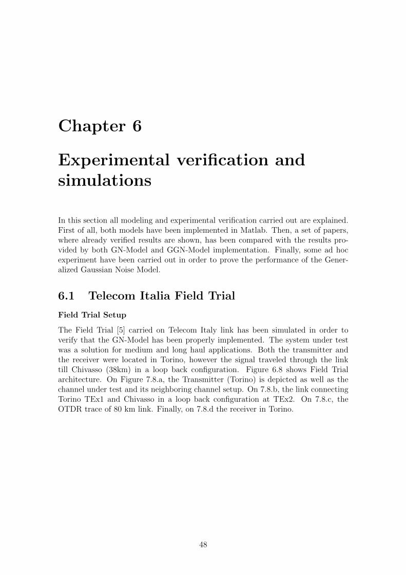
The Field Trial [5] carried on Telecom Italy link has been simulated in order toverify that the GN-Model has been properly implemented. The system under testwas a solution for medium and long haul applications. Both the transmitter andthe receiver were located in Torino, however the signal traveled through the linktill Chivasso (38km) in a loop back configuration. Figure 6.8 shows Field Trialarchitecture. On Figure 7.8.a, the Transmitter (Torino) is depicted as well as thechannel under test and its neighboring channel setup. On 7.8.b, the link connectingTorino TEx1 and Chivasso in a loop back configuration at TEx2. On 7.8.c, theOTDR trace of 80 km link. Finally, on 7.8.d the receiver in Torino.
48
6.1. TELECOM ITALIA FIELD TRIAL
Figure 6.1: Field Trial Architecture. This figure has been taken from [5] (Fig. 1)
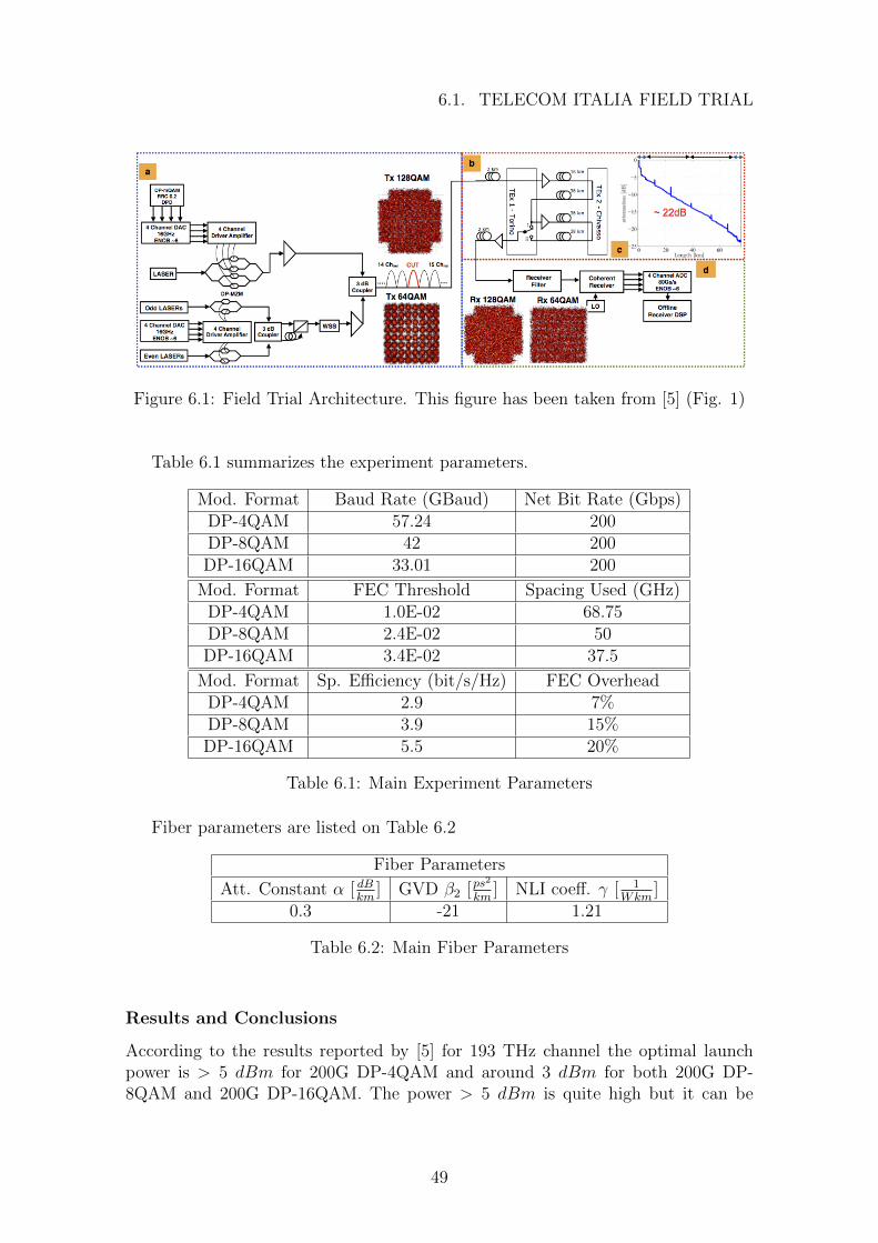
Table 6.1 summarizes the experiment parameters.
Mod. Format Baud Rate (GBaud) Net Bit Rate (Gbps)DP-4QAM 57.24 200DP-8QAM 42 200DP-16QAM 33.01 200
Mod. Format FEC Threshold Spacing Used (GHz)DP-4QAM 1.0E-02 68.75DP-8QAM 2.4E-02 50DP-16QAM 3.4E-02 37.5
Mod. Format Sp. Efficiency (bit/s/Hz) FEC OverheadDP-4QAM 2.9 7%DP-8QAM 3.9 15%DP-16QAM 5.5 20%
Table 6.1: Main Experiment Parameters
Fiber parameters are listed on Table 6.2
Fiber Parameters
Att. Constant ↵ [ dBkm
] GVD β2 [ps2
km] NLI coe↵. γ [ 1
Wkm]
0.3 -21 1.21
Table 6.2: Main Fiber Parameters
Results and Conclusions
According to the results reported by [5] for 193 THz channel the optimal launchpower is > 5 dBm for 200G DP-4QAM and around 3 dBm for both 200G DP-8QAM and 200G DP-16QAM. The power > 5 dBm is quite high but it can be
49
6.1. TELECOM ITALIA FIELD TRIAL
explained by the large bandwidth of the DP-4QAM 57.24 GBaud signal (for moreinformation about it: section ”results” [5]). The system was simulated accordingto three di↵erent models: GN-Model Approximated Formula, GN-Model and GGN-Model. The final expression for the three models are summarized below:
GNLI ⇡ 4
27
γ2Pch
⇡|β2|↵R3s
asinh⇣ 1
4↵⇡2|β2|R2
s[N2ch]
R
s
∆f
⌘(6.1)
GNLI(0) =64
27γ2NsL
2s,eff
Z BWDM
/2
0
⇢(⌫1, 0)χ(⌫1, 0)|2⌫1|Z log
e
(BWDM
/2⌫1)
0
hGWDM(⌫1e
⌫2)GWDM(⌫1e−⌫2)
hGWDM(2⌫1cosh(⌫2)) +GWDM(2⌫1sinh(⌫2))
id⌫2d⌫1 (6.2)
GNLI(f) =16
27γ2⇢(z, f)2
1Z
−1
1Z
−1
GTX(f1)GTX(f2)GTX(f1 + f2 − f)
(((zZ
0
ej4⇡2(f1−f)(f2−f)β2⇣
⇢(⇣, f1)⇢(⇣, f3)⇢(⇣, f2)
⇢(⇣, f)d⇣
(((2
df1df2 (6.3)
The verification process was carried out as follows:
Figure 2 of [5] compares theoretical BER and measured BER for di↵erent OSNR.The measured BER were obtained on a back-to-back configuration, i.e. on the ab-sence of optical link. Next table illustrates the minimum SNR in other to obtaineda given BER.
Mod. Format BER SNRsens[dB] OSNR [dB]DP-4QAM 1.0e-2 12.39 19DP-8QAM 2.4e-2 12.13 17.4DP-16QAM 3.4e-2 13.77 18
Table 6.3: Back-to-back values in terms of OSNR and SNR
Later, the number of span has been changed until the estimated SNR was asmuch as close to SNRsens. The reason the curves have stepped-like shape is thaton a real system the number of span should be an integer number. In other words,on theoretical analysis the maximum number of spans can be Ns=13.5, however,half span can be deployed on real systems. Figure 6.2 depicts the maximum lengthvariation against launch power.
50
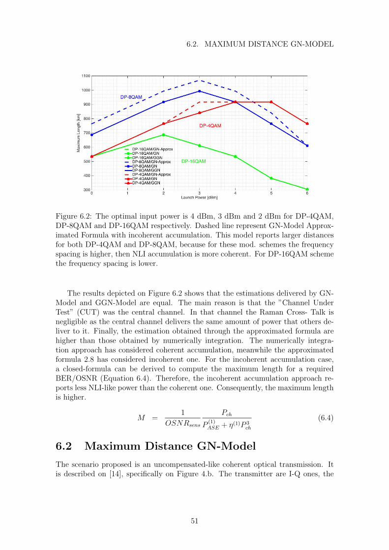
6.2. MAXIMUM DISTANCE GN-MODEL
Figure 6.2: The optimal input power is 4 dBm, 3 dBm and 2 dBm for DP-4QAM,DP-8QAM and DP-16QAM respectively. Dashed line represent GN-Model Approx-imated Formula with incoherent accumulation. This model reports larger distancesfor both DP-4QAM and DP-8QAM, because for these mod. schemes the frequencyspacing is higher, then NLI accumulation is more coherent. For DP-16QAM schemethe frequency spacing is lower.
The results depicted on Figure 6.2 shows that the estimations delivered by GN-Model and GGN-Model are equal. The main reason is that the ”Channel UnderTest” (CUT) was the central channel. In that channel the Raman Cross- Talk isnegligible as the central channel delivers the same amount of power that others de-liver to it. Finally, the estimation obtained through the approximated formula arehigher than those obtained by numerically integration. The numerically integra-tion approach has considered coherent accumulation, meanwhile the approximatedformula 2.8 has considered incoherent one. For the incoherent accumulation case,a closed-formula can be derived to compute the maximum length for a requiredBER/OSNR (Equation 6.4). Therefore, the incoherent accumulation approach re-ports less NLI-like power than the coherent one. Consequently, the maximum lengthis higher.
M =1
OSNRsens
Pch
P (1)ASE + ⌘(1)P 3
ch
(6.4)
6.2 Maximum Distance GN-Model
The scenario proposed is an uncompensated-like coherent optical transmission. Itis described on [14], specifically on Figure 4.b. The transmitter are I-Q ones, the
51

6.3. EXPERIMENT AT ORANGE LABORATORY
span length is 100 km, the amplification is lumped-like and the fiber used was Pure-silica-core fiber (PSCF). As it has been said on section 4.2 maximum distance isdefined as the distance such that satisfies a required SNR.The SNR is determinedby the required BER. Finally, back-to-back penalty should be taken into accountso that ISI and cross-talk noise are also considered. This parameter depends onmodulation format and how far away are the channels placed one from another. Thegreater the frequency spacing, the smaller the penalty. PM-8QAM SMF scenariofor di↵erent frequency spacing has been simulated, the simulated results provide thesame optimal launched power and maximum lengths as it is depicted on Figure 4.bof [14]. Figure 6.3 depicts the results reported by my implementation.
Figure 6.3: Maximum length for di↵erent input powers. SMF-QPSK case
The optimal launched power for all frequency spacing is around 0 dBm.
6.3 Experiment at Orange Laboratory
We simulate the experiment described in [15]. On this paper the GGN-Model wasverified with experimental results and then enables us to use it.
6.3.1 Laboratory Setup
The optical link consists on 20 spans of 80 km each. The optical fiber is CorningSMF -28e+. 58 channels were configured, 7 of those were commercial 100 Gb/stransponders and 51 came from a comb of lasers modulated by two 28 GBaud/s100 Gb/s laboratory transmitters. At the beginning, a WSS was used to combinethe channels as well as after span number 6 and 13 in order to flatten the signalspectrum.
52
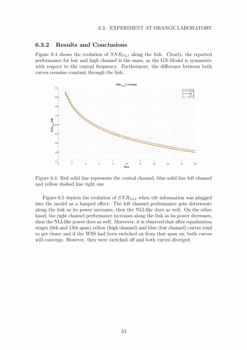
6.3. EXPERIMENT AT ORANGE LABORATORY
6.3.2 Results and Conclusions
Figure 6.4 shows the evolution of SNRNLI along the link. Clearly, the reportedperformance for low and high channel is the same, as the GN-Model is symmetricwith respect to the central frequency. Furthermore, the di↵erence between bothcurves remains constant through the link.
Figure 6.4: Red solid line represents the central channel, blue solid line left channeland yellow dashed line right one
Figure 6.5 depicts the evolution of SNRNLI when tilt information was pluggedinto the model as a lumped e↵ect. The left channel performance gets deterioratealong the link as its power increases, then the NLI-like does as well. On the otherhand, the right channel performance increases along the link as its power decreases,then the NLI-like power does as well. Moreover, it is observed that after equalizationstages (6th and 13th span) yellow (high channel) and blue (low channel) curves tendto get closer and if the WSS had been switched on from that span on, both curveswill converge. However, they were switched o↵ and both curves diverged.
53

6.3. EXPERIMENT AT ORANGE LABORATORY
Figure 6.5: Red solid line represents the central channel, blue solid line left channeland yellow solid line right one. It is observed that equalization stages are placed on6th and 13th spans.
Finally, the performance at the end of the link is depicted on Figure 6.6. Sameresults as in [15] has been obtained for Strategy 1 and Strategy 2. Strategy 1 refersto the broadly used GN-Model with incoherent accumulation, assuming flat launchpower at the input of each span. Strategy 2 improves the previous strategy byplugging tilt information into the model. The tilt information was composed ofboth the fiber loss and the cross-talk due to SRS. The latter has been estimatedfor a common peak polarization-averaged Raman efficiency value for SMF of 0.391/W/km. Furthermore, after the 6th and 13th span the equalization stage is added.Strategy 1 matches correctly with the measured values at the central frequency,however, it fails on side channels. For Strategy 2, the performance becomes closerto the real one. However, the slope is not well estimated. As a result, the GGN-Model is highly needed to estimate the side channel for no tilt compensation system.The GGN-Model was not simulated for 58 channels, but 31 channels in order to makethe simulation faster with the available resources. It is important to highlight that50% of total NLI PSD is generated by around 4 channels for 20 spans (see Figure2.5). Furthermore, the normalized, respect 101 channels, generated NLI PSD is 0.82for 31 channels and 0.9 for 58 channels. Therefore, the analysis can be consideredequivalent. Figure 6.7 depicts the values reported by GN and GGN-Model for 31Channels.
54

6.3. EXPERIMENT AT ORANGE LABORATORY
Figure 6.6: Red solid line represents the central channel, blue solid line left channeland yellow solid line right one
Figure 6.7: Blue solid line represents GN-Model and green solid line representsGGN-Model. GN-Model reports an over estimation at 193.5 THz with respect toGGN-Model and an under estimation at 194.5 THz with respect to GGN-Model.
Di↵erence between GGN-Model and GN-Model reported by [15] at 193.5 THzand 194.5 THz is around 0.7 and 0.5 dB respectively. My own simulations reports0.7 and 0.4 dB respectively.
55
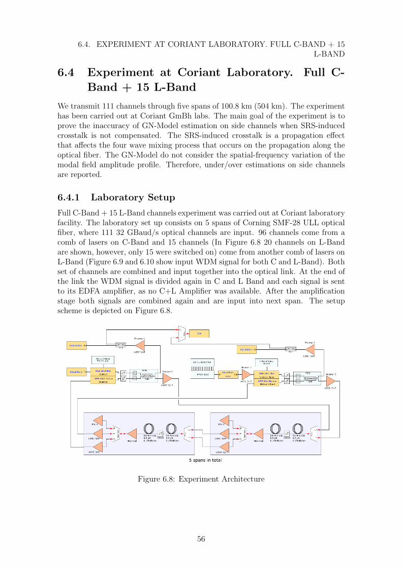
6.4. EXPERIMENT AT CORIANT LABORATORY. FULL C-BAND + 15L-BAND
6.4 Experiment at Coriant Laboratory. Full C-Band + 15 L-Band
We transmit 111 channels through five spans of 100.8 km (504 km). The experimenthas been carried out at Coriant GmBh labs. The main goal of the experiment is toprove the inaccuracy of GN-Model estimation on side channels when SRS-inducedcrosstalk is not compensated. The SRS-induced crosstalk is a propagation e↵ectthat a↵ects the four wave mixing process that occurs on the propagation along theoptical fiber. The GN-Model do not consider the spatial-frequency variation of themodal field amplitude profile. Therefore, under/over estimations on side channelsare reported.
6.4.1 Laboratory Setup
Full C-Band + 15 L-Band channels experiment was carried out at Coriant laboratoryfacility. The laboratory set up consists on 5 spans of Corning SMF-28 ULL opticalfiber, where 111 32 GBaud/s optical channels are input. 96 channels come from acomb of lasers on C-Band and 15 channels (In Figure 6.8 20 channels on L-Bandare shown, however, only 15 were switched on) come from another comb of lasers onL-Band (Figure 6.9 and 6.10 show input WDM signal for both C and L-Band). Bothset of channels are combined and input together into the optical link. At the end ofthe link the WDM signal is divided again in C and L Band and each signal is sentto its EDFA amplifier, as no C+L Amplifier was available. After the amplificationstage both signals are combined again and are input into next span. The setupscheme is depicted on Figure 6.8.
Figure 6.8: Experiment Architecture
56

6.4. EXPERIMENT AT CORIANT LABORATORY. FULL C-BAND + 15L-BAND
Figure 6.9: Input 96 Channels C-Band
Figure 6.10: Input 15 Channels L-Band
Table 6.4 reports the fiber parameters provided by the manufacturer.
Attenuation Constant ↵ Dispersion Parameter D Non-Linear Coefficient γ0.16 (dB/km) 18.1 (ps/nm/km) 1.0088 (1/W/km)
Table 6.4: Main Fiber Parameters
Table 6.5 reports the system parameters.
57

6.4. EXPERIMENT AT CORIANT LABORATORY. FULL C-BAND + 15L-BAND
Symbol Rate Roll-o↵ factor Modulation Format FEC Overhead32 (GBaud/s) 0.15 QPSK 15 %
Table 6.5: System Parameters
The values depicted on Table 6.4 are averaged values reported by the manufac-turer available on the data-sheet. However, the exact loss produced at each span hasbeen measured (WWG OLP-18C Power Meter). It is critical to be accurate on theinput power at each span, as a small variance on the input power value can a↵ectsubstantially to the NLI-power estimate.Table 6.6 depicts the loss at each span and the loss source.
Span Device Loss [dB]1 C+L Combiner 0.631 Fiber 16.61 PRC-4LP + Splitter 1.82 C+L Combiner 0.72 Fiber 16.92 PRC-4LP + Splitter 2.33 C+L Combiner 0.753 Fiber 16.653 PRC-4LP + Splitter 2.24 C+L Combiner 0.74 Fiber 16.94 PRC-4LP + Splitter 0.635 C+L Combiner 0.555 Fiber 16.455 PRC-4LP + Splitter 2.23
Table 6.6: Span Losses
The SRS cross talk causes a power di↵erence of around 8 dB (C-Band) and 1 dB(L-Band) between low frequency channels and high frequency after 502 km. Theripple caused by the EDFA masked a bit the SRS-e↵ect on L-Band. Figure 6.11 and6.12 illustrate the output spectrum.
58
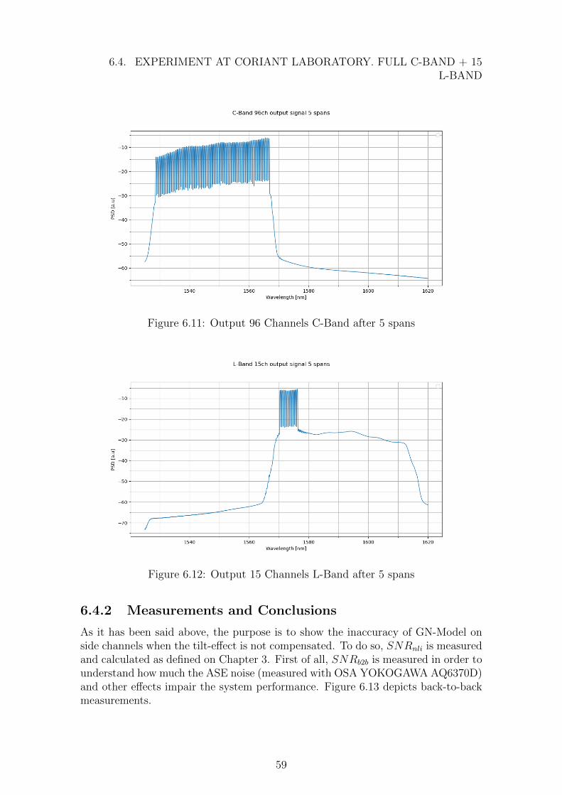
6.4. EXPERIMENT AT CORIANT LABORATORY. FULL C-BAND + 15L-BAND
Figure 6.11: Output 96 Channels C-Band after 5 spans
Figure 6.12: Output 15 Channels L-Band after 5 spans
6.4.2 Measurements and Conclusions
As it has been said above, the purpose is to show the inaccuracy of GN-Model onside channels when the tilt-e↵ect is not compensated. To do so, SNRnli is measuredand calculated as defined on Chapter 3. First of all, SNRb2b is measured in order tounderstand how much the ASE noise (measured with OSA YOKOGAWA AQ6370D)and other e↵ects impair the system performance. Figure 6.13 depicts back-to-backmeasurements.
59

6.4. EXPERIMENT AT CORIANT LABORATORY. FULL C-BAND + 15L-BAND
Figure 6.13: Back-to-back measurements
According to the back-to-back measurements, it is clearly observed that the re-ceiver saturates at maximum SNR equal to around 20 dB. Then, when non-lineare↵ects does not impair the performance (back-to-back), there are other e↵ects be-yond the ASE noise. Therefore, the back-to-back definition explained on Chapter4 must be recast. Instead of SNRb2b = Pch/Pase, SNRb2b is redefined taking intoaccount receiver impairments as SNRb2b = Pch/(Pase +Pothers). These impairmentsare named Pothers since their sources are out of the scope of this thesis. The sourcescan be quantification noise or electrical noise. The method of measurement is de-fined as follows: The output OSNR is measured after five spans. Later, the receivermeasures the so-called EVM defined in 4.1, which relates the signal and the errorpower. This magnitude considers both ASE noise, receiver and non-linear e↵ects.After some mathematical computations non-linear impairments can be analyzed.
SNRrx =Pch
Pase + Pothers + Pnli
1
SNRrx
=Pase + Pothers + Pnli
Pch
1
SNRrx
=1
SNRnli
+1
SNRb2b
1
SNRnli
=1
SNRrx
− 1
SNRb2b(6.5)
The strategies used to compute NLI-power are Strategy 1 and 2 defined on previoussection. Strategy 1 compute only compute GN-Model at the beginning of first spanand assumes that the accumulation is incoherent. Furthermore, Strategy 1 assumesthat the spectrum remains flat through the whole link. In other words, Strategy
60
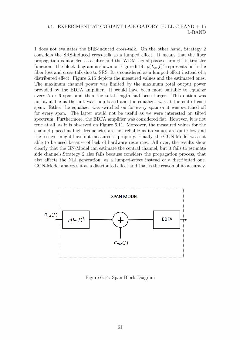
6.4. EXPERIMENT AT CORIANT LABORATORY. FULL C-BAND + 15L-BAND
1 does not evaluates the SRS-induced cross-talk. On the other hand, Strategy 2considers the SRS-induced cross-talk as a lumped e↵ect. It means that the fiberpropagation is modeled as a filter and the WDM signal passes through its transferfunction. The block diagram is shown on Figure 6.14. ⇢(Ls, f)2 represents both thefiber loss and cross-talk due to SRS. It is considered as a lumped-e↵ect instead of adistributed e↵ect. Figure 6.15 depicts the measured values and the estimated ones.The maximum channel power was limited by the maximum total output powerprovided by the EDFA amplifier. It would have been more suitable to equalizeevery 5 or 6 span and then the total length had been larger. This option wasnot available as the link was loop-based and the equalizer was at the end of eachspan. Either the equalizer was switched on for every span or it was switched o↵for every span. The latter would not be useful as we were interested on tiltedspectrum. Furthermore, the EDFA amplifier was considered flat. However, it is nottrue at all, as it is observed on Figure 6.11. Moreover, the measured values for thechannel placed at high frequencies are not reliable as its values are quite low andthe receiver might have not measured it properly. Finally, the GGN-Model was notable to be used because of lack of hardware resources. All over, the results showclearly that the GN-Model can estimate the central channel, but it fails to estimateside channels.Strategy 2 also fails because considers the propagation process, thatalso a↵ects the NLI generation, as a lumped-e↵ect instead of a distributed one.GGN-Model analyzes it as a distributed e↵ect and that is the reason of its accuracy.
Figure 6.14: Span Block Diagram
61

6.4. EXPERIMENT AT CORIANT LABORATORY. FULL C-BAND + 15L-BAND
Figure 6.15: Blue solid line represents Strategy 1 and red solid line represents Strat-egy 2. Yellow bars represent +/- 1 dB around the measured value. In other words,an estimation inside the interval [xmeasured − 1, xmeasured + 1] is accepted.
Finally, ⌘nl parameter allow us to verify if SNRnli was properly measured. Thisparameter is defined as [6]:
⌘nl = (1/SNRnli)/(Pch −∆P )2 (6.6)
∆P = 0.75 dB and is equivalent to connector loss. Connector losses leads that theinput power into the fiber is no exactly the expected one. Furthermore, NLI powervaries with the cube of the input power. Therefore, a small di↵erence on the inputpower leads to a high di↵erence on the NLI power. ⌘nl should be constant. Figure6.16 shows both ⌘measured and ⌘simulated.
62

6.5. 15 CHANNELS ON C-BAND AND 35 CHANNELS ON L-BAND
Figure 6.16: Measure for channel at 193.75 THz. Square-like dots represents themeasurements of ⌘nl and solid red line the simulated one. 0.5 dB maximum di↵erenceamong measurements is reported.
The di↵erence between the averaged measured value and the simulated one isaround 0.3 dB, which is an acceptable di↵erence.
6.5 15 Channels on C-Band and 35 Channels onL-Band
Coriant lab scenario was simulated in order to obtain the maximum length reachablewhen 50 channels are input into the system. 15 of theses are placed on L-Band (from190.2 THz to 190.9 THz) and 35 are placed on C-Band (191.35 THz to 193.05 THz).The laboratory setup is almost like the one used on section 6.4. However, the signalpower is equalized every 5 spans. Last five spans were not equalized in order to seethe SRS cross-talk e↵ect. Then, PM-QPSK signals at 32 GBaud/s are transmitted,the channels are separated 50 GHz and the fiber is Corning SMF-28 ULL. Thepurpose of this simulation is to evaluate the maximum distance achievable by thesystem under the conditions summarized above. Table summarized the relationbetween three di↵erent BER values and their minimum required SNR.
Bit Error Rate (BER) Signal-to-Noise Ratio (SNR)1.19E-02 7.3 dB5.50E-03 8.35 dB8.55E-03 10.15 dB
Table 6.7: BER-SNR
63

6.5. 15 CHANNELS ON C-BAND AND 35 CHANNELS ON L-BAND
Channel number 3 (190.3 THz) and channel number 33 (191.8 THz) were an-alyzed. The metric used to study the system performance is the Signal-to-NoiseRatio as described in Chapter 4. The NLI noise-like power was computed throughboth GN-Model and GGN-Model. As expected, for the channel placed on L-Bandthe GN-Model failed. For instance, the maximum distance reported by GN-Model,in order to obtain a BER equal to 5.50E-03 at the receiver side, is 2000 km greaterthan that reported by GGN-Model. Figure 6.17
Figure 6.17: Blue solid line GGN-Model at 190.3 THz, blue dashed line GN-Modelat 190.3, green solid line GGN-Model at 191.8 THz and green dashed line GN-Modelat 191.THz. Both models report similar values at 191.8 THz.On the other hand,GN-Model fails at 190.3 THz.
64

Chapter 7
Conclusions
The final chapter entitled ”Conclusions” is devoted to summarized main resultsobtained and to highlight futures developments to be carried out. Through thisMaster Thesis Project, GN-Model and GGN-Model have been analyzed and com-pared. Both models were implemented in order to carry out simulations to estimatethe performance of an optical system through signal-to-noise ratio. Thus, the per-formance is measured in terms of Quality of Transmission of the physical layer.
Regarding the implementation and coding efficiency, one of the key point is thenumber of samples definition to solve the spatial integral for GGN-Model. It hasbeen proved that incorrect estimates are reported if this value is not properly cho-sen. One possibility for futures implementations is to set the number of samplesdynamically as it has been proved in this thesis that the optimal one changes a lotwhen the spectral components involved in Four-Wave-Mixing process are close tothe frequency under analysis and when they are further in terms of frequency. Thegoal should be to improve the solution of the numerical integral.
Regarding the system performance estimation, it has been demonstrated that GN-Model is still accurate for the central channel of C-Band even if few channels whereadded on L-Band (15 Channels). However, it fails on side channels of C-Band dueto cross-talk produced by Stimulated Raman Scattering. Measurements on L-Bandwould also be interesting in order to verify GN-Model reliability on this L-Band,whose commercial interest is growing every year.
Finally, GGN-Model estimates with high accuracy channels a↵ected by cross-talkdue to Stimulated Raman Scattering. In other words, GGN-Model considers thise↵ect as distributed and its results are much better than the GN-Model, which con-siders it as a lumped e↵ect. In terms of maximum distance estimation, GN-Modelover-estimated in 2000 km the result provided by GGN-Model for a C+L system. Inmy opinion, future developments should be focus on testing GGN-Model on L-Band.
65

Appendices
66

Appendix A
Matlab Files
GN-Model. Hyperbolic Coordinates
Here it is shown the GN-Model in Hyperbolic Coordinates
1 % @Author : Angel Alonso2 % Company : Coriant GmbH Muenchen3 % Unives i ty : Po l i t e c n i c o d i Torino & Univers idad Po l i t e c n i c a
de Madrid4
5 % This r e tu rn s NLI PSD at f .6 % I t uses Hyperbo l i c Coordinates7 % Bib l iography : P i e r l u i g i Pogg i o l i n i : ”Th GN Model o f Non−
Linear Propagation8 % in Uncompensated
Coherent Opt ica l Systems”9
10 %============================================================
11 % INPUT12 %
============================================================
13 %14 % fiberParams : Type : St ruct . I t conta in s f i b e r parameters (
alpha , beta2 and gamma)15 % s i g n a l : Type : St ruct . I t conta in s s i g n a l parameters ( power
, r o l l−o f f ,Bw and Rs)16 % sys : Type : St ruct . I t conta in s system parameters ( number
o f channels ,17 % span length , number o f spans , bw, EDFA Gain , Figure Noise )
67

18 % f : Type : Double . Frequency under an a l y s i s . Baseband . f=0c en t r a l channel [THz ]
19 % gtx : Type : Double Array . WDM Signa l Spectrum [W/Hz ]20 %21 %
============================================================
22 % OUTPUT23 %
============================================================
24 %25 % GNLI0 : Type : Double . NLI PSD at f [W/Hz ]26
27
28 f unc t i on GNLI0=GNLI f hyp ( f iberParams , s i gna l , sys , f , gtx )29 nSamples = f l o o r ( sys .Bw⇤23000/2) ;30 f r e q = l i n s p a c e (− sys .Bw/2 , sys .Bw/2 , nSamples ) ;31 % gtx = GTX( s i gna l , sys , f r e q ) ;32 % Parameters33 Le f f = (1−exp(−2⇤ f iberParams . alpha⇤ sys . Ls ) ) /(2⇤
f iberParams . alpha ) ; % E f f e c t i v e span length34 r e s o l v 1 =16; % After eva lua t ing the i n t e g r a l
convergence . Our r e s o l u t i o n along v1 i s 16samples /GHz
35 nSamplesv1=f l o o r ( r e s o l v 1 ⇤ sys .Bw⇤1000) ;36 % Let ’ s compute GNRF at f=037 v1=l i n s p a c e (0 , sys .Bw,2⇤ nSamplesv1 ) ;38 %pace=v1 (2 ) ;39 p0num=1−exp(−2⇤ f iberParams . alpha⇤ sys . Ls )⇤exp (1 i ⇤4⇤ pi
ˆ2⇤ f iberParams .GVD⇤ sys . Ls⇤v1 . ˆ 2 ) ;40 p0dem=2⇤ f iberParams . alpha−1 i ⇤4⇤ pi ˆ2⇤ f iberParams .GVD⇤
v1 . ˆ 2 ;41 p0=abs (p0num./ p0dem) . ˆ 2 ; %FWM e f f i c i e n c y f o r f=042 p0=p0/( Le f f ˆ2) ;43 p0=10⇤ l og10 ( p0 ) ;44 th=−30; % Threshold to speed up the numer ica l
i n t e g r a t i o n . The bigger , the f a s t e r .45 ind=f i nd (p0>=th ) ;46 p0=p0 ( ind ) ;47 p0=10.ˆ(p0 /10) ;48 v1=v1 ( ind ) ;49 x0num=s in (2⇤ sys . Ns⇤ pi ˆ2⇤v1 .ˆ2⇤ f iberParams .GVD⇤ sys . Ls
) . ˆ 2 ;
68

50 x0dem=s in (2⇤ pi ˆ2⇤v1 .ˆ2⇤ f iberParams .GVD⇤ sys . Ls ) . ˆ 2 ;51 x0=x0num ./ x0dem ;52 x0 (1 )=sys . Ns ˆ2 ;53
54 A=p0 .⇤ x0 .⇤ abs (2⇤v1 ) ;55 A=A/max(A) ;56 A=10⇤ l og10 (A) ;57 ind2 = f i nd (A<−20) ;58 Gnli0=ze ro s (1 , l ength ( v1 ) ) ;59 f p r i n t f ( ’ Processed 0%%’ )60 f o r j j =1: l ength ( v1 )61 i f ( j j ==1)62 v2upLim=log ( sys .Bw/(0 . 0001 ) ) ;63 e l s e64 v2upLim = log ( sys .Bw/( v1 ( j j ) ) ) ;65 end66 i f ismember ( j j , ind2 )67
68 e l s e69 v2 = l i n s p a c e (0 , v2upLim , nSamplesv1 ) ;70 f r eq01 = v1 ( j j ) .⇤ exp ( v2 )+f ;71 f r eq02 = v1 ( j j ) .⇤ exp(−v2 )+f ;72 f r eq03 = 2⇤v1 ( j j ) .⇤ cosh ( v2 )+f ;73 f r eq04 = −v1 ( j j ) .⇤ exp(−v2 )+f ;74 f r eq05 = 2⇤v1 ( j j )⇤ s inh ( v2 )+f ;75 f r eq06 = −v1 ( j j ) .⇤ exp ( v2 )+f ;76 f r eq07 = −2⇤v1 ( j j ) .⇤ s inh ( v2 )+f ;77 f r eq08 = −2⇤v1 ( j j ) .⇤ cosh ( v2 )+f ;78 g01 = in t e rp1 ( f r eq , gtx , f req01 , ’ cub ic ’ ) ;79 g02 = in t e rp1 ( f r eq , gtx , f req02 , ’ cub ic ’ ) ;80 g03 = in t e rp1 ( f r eq , gtx , f req03 , ’ cub ic ’ ) ;81 g04 = in t e rp1 ( f r eq , gtx , f req04 , ’ cub ic ’ ) ;82 g05 = in t e rp1 ( f r eq , gtx , f req05 , ’ cub ic ’ ) ;83 g06 = in t e rp1 ( f r eq , gtx , f req06 , ’ cub ic ’ ) ;84 g07 = in t e rp1 ( f r eq , gtx , f req07 , ’ cub ic ’ ) ;85 g08 = in t e rp1 ( f r eq , gtx , f req08 , ’ cub ic ’ ) ;86 I0=g01 .⇤ g02 .⇤ g03+g01 .⇤ g04 .⇤ g05+g06 .⇤ g02 .⇤ g07
+g06 .⇤ g04 .⇤ g08 ;87 Gnli0 ( j j )=trapz ( v2 , I0 ) ; %Inner i n t e g r a l .
I n t e g r a t i on domain over v288 end89 i f mod( j j , 100) == 090 f p r i n t f ( ’ \b\b\b%g%%’ , round ( j j ⇤100/ l ength ( v1
) ) )
69
91 end92 end93 I I=p0 .⇤ x0 .⇤ Gnli0 .⇤ abs (2⇤v1 ) ;94 GNLI0=trapz ( v1 , I I ) ; %Outer i n t e r g r a l . I n t e g r a t i on
domain over v195 GNLI0=(32/27) ⇤( f iberParams .gammaˆ2) ⇤( L e f f ˆ2)⇤GNLI0⇤1
e−12; % PSD in W/Hz96
97 end
GN-Model. Hyperbolic Coordinates at f=0
Here it is shown the GN-Model in Hyperbolic Coordinates at f=0
1 % @Author : Angel Alonso2 % Company : Coriant GmbH Muenchen3 % Unives i ty : Po l i t e c n i c o d i Torino & Univers idad Po l i t e c n i c a
de Madrid4
5 % This r e tu rn s NLI PSD at f .6 % I t uses Cartes ian Coordinates7 % Bib l iography : P i e r l u i g i Pogg i o l i n i : ”Th GN Model o f Non−
Linear Propagation8 % in Uncompensated
Coherent Opt ica l Systems”9
10 %============================================================
11 % INPUT12 %
============================================================
13 %14 % fiberParams : Type : St ruct . I t conta in s f i b e r parameters (
alpha , beta2 and gamma)15 % s i g n a l : Type : St ruct . I t conta in s s i g n a l parameters ( power
, r o l l−o f f ,Bw and Rs)16 % sys : Type : St ruct . I t conta in s system parameters ( number
o f channels ,17 % span length , number o f spans , bw, EDFA Gain , Figure Noise )18 %19 %
============================================================
70

20 % OUTPUT21 %
============================================================
22 %23 % GNLI0 : Type : Double . NLI PSD at f [W/Hz ]24
25 f unc t i on GNLI0=GNLI 0 hyp ( f iberParams , s i gna l , sys )26 nSamples = f l o o r ( sys .Bw⇤23000/2) ;27 f = l i n s p a c e (− sys .Bw/2 , sys .Bw/2 , nSamples ) ;28 gtx = GTX( s i gna l , sys , f ) ;29 % Parameters30 Le f f = (1−exp(−2⇤ f iberParams . alpha⇤ sys . Ls ) ) /(2⇤ f iberParams .
alpha ) ; % E f f e c t i v e span length31 r e s o l v 1 =16; % After eva lua t ing the i n t e g r a l convergence . Our
r e s o l u t i o n along v1 i s 16 samples /GHz32 nSamplesv1=f l o o r ( r e s o l v 1 ⇤ sys .Bw⇤1000) ;33 % Let ’ s compute GNRF at f=034 v1=l i n s p a c e (0 , sys .Bw/2 , nSamplesv1 ) ;35 %pace=v1 (2 ) ;36 p0num=1−exp(−2⇤ f iberParams . alpha⇤ sys . Ls )⇤exp (1 i ⇤4⇤ pi ˆ2⇤
f iberParams .GVD⇤ sys . Ls⇤v1 . ˆ 2 ) ;37 p0dem=2⇤ f iberParams . alpha−1 i ⇤4⇤ pi ˆ2⇤ f iberParams .GVD⇤v1 . ˆ 2 ;38 p0=abs (p0num./ p0dem) . ˆ 2 ; %FWM e f f i c i e n c y f o r f=039 p0=p0/( Le f f ˆ2) ;40 p0=10⇤ l og10 ( p0 ) ;41 th=−30; % Threshold to speed up the numer ica l i n t e g r a t i o n .
The bigger , the f a s t e r .42 ind=f i nd (p0>=th ) ;43 p0=p0 ( ind ) ;44 p0=10.ˆ(p0 /10) ;45 v1=v1 ( ind ) ;46 x0num=s in (2⇤ sys . Ns⇤ pi ˆ2⇤v1 .ˆ2⇤ f iberParams .GVD⇤ sys . Ls ) . ˆ 2 ;47 x0dem=s in (2⇤ pi ˆ2⇤v1 .ˆ2⇤ f iberParams .GVD⇤ sys . Ls ) . ˆ 2 ;48 x0=x0num ./ x0dem ;49 x0 (1 )=sys . Ns ˆ2 ;50
51 A=p0 .⇤ x0 .⇤ abs (2⇤v1 ) ;52 A=A/max(A) ;53 A=10⇤ l og10 (A) ;54 ind2 = f i nd (A<−20) ;55 Gnli0=ze ro s (1 , l ength ( v1 ) ) ;56 f o r j j =1: l ength ( v1 )
71

57 i f ( j j ==1)58 v2upLim=log ( sys .Bw/(2⇤0 .0001) ) ;59 e l s e60 v2upLim = log ( sys .Bw/(2⇤v1 ( j j ) ) ) ;61 end62 i f ismember ( j j , ind2 )63
64 e l s e65 v2 = l i n s p a c e (0 , v2upLim , nSamplesv1 ) ;66 f r eq01 = v1 ( j j )⇤exp ( v2 ) ;67 f r eq02 = v1 ( j j )⇤exp(−v2 ) ;68 f r eq03 = 2⇤v1 ( j j )⇤ cosh ( v2 ) ;69 f r eq05 = 2⇤v1 ( j j )⇤ s inh ( v2 ) ;70 max f01 = max( f r eq01 ) ;71 max f02 = max( f r eq02 ) ;72 max f03 = max( f r eq03 ) ;73 max f05 = max( f r eq05 ) ;74 min f01 = min ( f r eq01 ) ;75 min f02 = min ( f r eq02 ) ;76 min f03 = min ( f r eq03 ) ;77 min f05 = min ( f r eq05 ) ;78 i f or (max f01<−sys .Bw/2 , min f01>sys .Bw/2)79 Gnli0 ( j j )=0;80 e l s e i f or (max f02<−sys .Bw/2 , min f02>sys .Bw/2)81 Gnli0 ( j j )=0;82 e l s e i f and ( or (max f03<−sys .Bw/2 , min f03>sys .Bw/2) , or
(max f05<−sys .Bw/2 , min f05>sys .Bw/2) )83 Gnli0 ( j j )=0;84 e l s e85 g01 = in t e rp1 ( f , gtx , f req01 , ’ cub ic ’ ) ;86 g02 = in t e rp1 ( f , gtx , f req02 , ’ cub ic ’ ) ;87 g03 = in t e rp1 ( f , gtx , f req03 , ’ cub ic ’ ) ;88 g05 = in t e rp1 ( f , gtx , f req05 , ’ cub ic ’ ) ;89 end90 I0=g01 .⇤ g02 . ⇤ ( g03+g05 ) ;91 Gnli0 ( j j )=trapz ( v2 , I0 ) ; %Inner i n t e g r a l . I n t e g r a t i on
domain over v292 end93 i f mod( j j , 100) == 094 f p r i n t f ( ’%g%% \n ’ , round ( j j ⇤100/ l ength ( v1 ) ) )95 end96 end97 I I=p0 .⇤ x0 .⇤ Gnli0 .⇤ abs (2⇤v1 ) ;
72
98 GNLI0=trapz ( v1 , I I ) ; %Outer i n t e r g r a l . I n t e g r a t i on domainover v1
99 GNLI0=(64/27) ⇤( f iberParams .gammaˆ2) ⇤( L e f f ˆ2)⇤GNLI0⇤1e−12; %PSD in W/Hz
100
101 end
GN-Model. Cartesian Coordinates
Here it is shown the GN-Model in Cartesian Coordinates
1 % @Author : Angel Alonso2 % Company : Coriant GmbH Muenchen3 % Unives i ty : Po l i t e c n i c o d i Torino & Univers idad Po l i t e c n i c a
de Madrid4
5 % This r e tu rn s NLI PSD at f .6 % I t uses Cartes ian Coordinates7 % Bib l iography : P i e r l u i g i Pogg i o l i n i : ”Th GN Model o f Non−
Linear Propagation8 % in Uncompensated
Coherent Opt ica l Systems”9
10 %============================================================
11 % INPUT12 %
============================================================
13 %14 % fiberParams : Type : St ruct . I t conta in s f i b e r parameters (
alpha , beta2 and gamma)15 % s i g n a l : Type : St ruct . I t conta in s s i g n a l parameters ( power
, r o l l−o f f ,Bw and Rs)16 % sys : Type : St ruct . I t conta in s system parameters ( number
o f channels ,17 % span length , number o f spans , bw, EDFA Gain , Figure Noise )18 % f : Type : Double . Frequency under an a l y s i s . Baseband . f=0
c en t r a l channel [THz ]19 % gtx : Type : Double Array . WDM Signa l Spectrum [W/Hz ]20 %21 %
============================================================
73

22 % OUTPUT23 %
============================================================
24 %25 % GNLI : Type : Double . NLI PSD at f [W/Hz ]26
27
28 f unc t i on GNLI = GNLI f ( f iberParams , s i gna l , sys , f , gtx )29 nSamples = f l o o r ( sys .Bw⇤23000/8) ;30 f 2 = l i n s p a c e (− sys .Bw/2 , sys .Bw/2 , nSamples ) ;31 f 1 = l i n s p a c e (− sys .Bw/2 , sys .Bw/2 , nSamples ) ;32
33 da = −2⇤ f iberParams . alpha ;34 g t x f 2 = gtx ;35 g t x f 1 = g tx f 2 ;36 I2 = ze ro s (1 , nSamples ) ;37 n=nSamples ;38 [ c , index ] = min ( abs ( f−f 2 ) ) ;39 f o r j j = 1 : n40 db = 1 i ⇤4⇤ pi ˆ2⇤( f 1 ( j j )−f ) ⇤( f2−f )⇤ f iberParams .GVD;41 p1=abs ((1−exp ( da⇤ sys . Ls ) .⇤ exp (db⇤ sys . Ls ) ) ./(−da−db) )
. ˆ 2 ;42 i f sys . Ns == 143 ch i = ones (1 , nSamples ) ;44 e l s e45 ch i = ( s i n (db ./2⇤ sys . Ns⇤ sys . Ls ) . / s i n (db ./2⇤ sys . Ls ) )
. ˆ 2 ;46 end47 vec2 = f i nd (db==0) ;48 ch i ( vec2 ) = sys . Ns ˆ2 ;49 i f index−j j>=050 ze = ze ro s (1 , index− j j ) ;51 g t x f 3 = horzcat ( ze , g t x f 2 ( 1 : ( n−l ength ( ze ) ) ) ) ;52 I2 ( j j )=trapz ( f2 , p1 .⇤ ch i .⇤ g t x f 1 ( j j ) .⇤ g t x f 2 .⇤
g t x f 3 ) ;53 e l s e54 ze = ze ro s (1 , abs ( index− j j ) ) ;55 g t x f 3 = horzcat ( g t x f 2 (1+ length ( ze ) : end ) , ze ) ;56 I2 ( j j )=trapz ( f2 , p1 .⇤ ch i .⇤ g t x f 1 ( j j ) .⇤ g t x f 2 .⇤
g t x f 3 ) ;57 end58
74

59 i f mod( j j , 100) == 060 f p r i n t f ( ’%g%% \n ’ , round ( j j ⇤100/nSamples ) )61 end62
63 end64 save ( ’FUNCTION.mat ’ , ’ I2 ’ ) ;65 I1 = trapz ( f1 , I2 ) ;66 GNLI=16/27⇤ f iberParams .gammaˆ2⇤ I1 ⇤1e−12;67
68 end
GGN-Model. Matrix Approach
Here it is shown the GGN-Model
1 % @Author : Angel Alonso2 % Company : Coriant GmbH Muenchen3 % Unives i ty : Po l i t e c n i c o d i Torino & Univers idad Po l i t e c n i c a
de Madrid4
5 % This r e tu rn s NLI PSD at f .6 %
============================================================
7 % INPUT8 %
============================================================
9 %10 % fiberParams : Type : St ruct . I t conta in s f i b e r parameters (
alpha , beta2 and gamma)11 % s i g n a l : Type : St ruct . I t conta in s s i g n a l parameters ( power
, r o l l−o f f ,Bw and Rs)12 % sys : Type : St ruct . I t conta in s system parameters ( number
o f channels ,13 % span length , number o f spans , bw, EDFA Gain , Figure Noise )14 % f : Type : Double . Frequency under an a l y s i s . Baseband . f=0
c en t r a l channel [THz ]15 % f i bP r o f : Double Matrix Type . Power evo lu t i on p r o f i l e16 % sigPSD : Double Array . WDM Signa l Spectrum [W/Hz ]17 % zeta sample s : Double Type . I t s e t the number o f samples o f
z18 %
75
19 %============================================================
20 % OUTPUT21 %
============================================================
22 %23 % GGf : Type : Double . NLI PSD at f [W/Hz ]24
25 f unc t i on GGf = GGNLI f ( f iberParams , s i gna l , sys , f , f i bPro f ,sigPSD , ze ta sample s )
26 nSamples=f l o o r ( sys .Bw⇤23000/8) ;27 f 2=l i n s p a c e (− sys .Bw/2 , sys .Bw/2 , nSamples ) ;28 f 1=l i n s p a c e (− sys .Bw/2 , sys .Bw/2 , nSamples ) ;29 g t x f 2 = sigPSD ;30 g t x f 1 = g tx f 2 ; % PSD S igna l f 131 I2 = ze ro s (1 , nSamples ) ; % Inner I n t e g r a l32 I I 2 = ze ro s (1 , nSamples ) ; % Inner I n t e g r a l33 n=nSamples ;34 [ c , index ] = min ( abs ( f−f 2 ) ) ;35 z = l i n s p a c e (0 , sys . Ls , z e ta sample s ) ;36 f i b = ze ro s (n , l ength ( z ) ) ;37 f o r i =1: l ength ( z )38 f i b ( : , i )=in t e rp1 ( sys . fCh , f i bP r o f ( : , i ) , f2 , ’ cub ic ’ ) ;39 end40 f i b f = f i b ( index , : ) ;41 f i b f = sq r t ( f i b f ) ;42 f i b f = repmat ( f i b f , n , 1 ) ;43
44 f o r j j =1:n45 i f mod( j j , 100) == 046 f p r i n t f ( ’%g%% \n ’ , round ( j j ⇤100/nSamples ) )47 end48 % f p r i n t f ( ’%g \n ’ , j j )49 i f g t x f 1 ( j j ) == 050 I2 ( j j ) = 0 ;51 e l s e52 f 3 =f1 ( j j )+f2−f ;53 i f index−j j>=054 ze = ze ro s (1 , index− j j ) ;55 db = 1 i ⇤4⇤ pi ˆ2⇤( f 1 ( j j )−f ) ⇤( f 2 ( ( index− j j +1) : end )−
f )⇤ f iberParams .GVD;56 db = reshape (db , l ength (db) ,1 ) ;
76

57 db = repmat (db , 1 , l ength ( z ) ) ;58 Z = repmat ( z , s i z e (db , 1 ) , 1 ) ;59 F = db .⇤Z ;60 F = exp (F) ;61 f i b f 1 = f i b ( j j , : ) ;62 f i b f 1 = sq r t ( f i b f 1 ) ;63 f i b f 1 = repmat ( f i b f 1 , s i z e (db , 1 ) , 1 ) ;64 f i b f 2 = sq r t ( f i b ) ;65 f i b f 3 = f i b f 2 ( 1 : ( n−l ength ( ze ) ) , : ) ;66 t e s t = f i b f 1 .⇤ f i b f ( ( index− j j +1) : end , : ) .⇤ f i b f 2
( ( index− j j +1) : end , : ) . / f i b f 3 ;67 F = F.⇤ t e s t ;68 F = trapz ( z ,F , 2 ) ;69 F = abs (F) . ˆ 2 ;70 F = horzcat ( ze ,F ’ ) ;71 g t x f 3 = horzcat ( ze , g t x f 2 ( 1 : ( n−l ength ( ze ) ) ) ) ;72 I2 ( j j )=trapz ( f2 ,F.⇤ g t x f 1 ( j j ) .⇤ g t x f 2 .⇤ g t x f 3 ) ;73
74 e l s e75 ze = ze ro s (1 , abs ( index− j j ) ) ;76 db = 1 i ⇤4⇤ pi ˆ2⇤( f 1 ( j j )−f ) ⇤( f 2 ( 1 : ( end−abs ( index−
j j ) ) )−f )⇤ f iberParams .GVD;77 db = reshape (db , l ength (db) ,1 ) ;78 db = repmat (db , 1 , l ength ( z ) ) ;79 Z = repmat ( z , s i z e (db , 1 ) , 1 ) ;80 F = db .⇤Z ;81 F = exp (F) ;82 f i b f 1 = f i b ( j j , : ) ;83 f i b f 1 = sq r t ( f i b f 1 ) ;84 f i b f 1 = repmat ( f i b f 1 , s i z e (db , 1 ) , 1 ) ;85 f i b f 3 = f i b f 2 ((1+ length ( ze ) ) : end , : ) ;86 t e s t = f i b f 1 .⇤ f i b f ( 1 : ( end−abs ( index− j j ) ) , : ) .⇤
f i b f 2 ( 1 : ( end−abs ( index− j j ) ) , : ) . / f i b f 3 ;87 F = F.⇤ t e s t ;88 F = trapz ( z ,F , 2 ) ;89 F = abs (F) . ˆ 2 ;90 F = horzcat (F ’ , ze ) ;91 g t x f 3 = horzcat ( g t x f 2 (1+ length ( ze ) : end ) , ze ) ;92 I2 ( j j )=trapz ( f2 ,F.⇤ g t x f 1 ( j j ) .⇤ g t x f 2 .⇤ g t x f 3 ) ;93 end94 end95 end96 save ( ’ I 2 1 2 j un e 2 .mat ’ , ’ I2 ’ ) ;97 I1=trapz ( f1 , I2 ) ;
77

98 GGf=16/27⇤ f iberParams .gammaˆ2⇤ I1 ⇤1e−12;99 end
GGN-Model. Loop/Matrix Approach
Here it is shown the GGN-Model
1 % @Author : Angel Alonso2 % Company : Coriant GmbH Muenchen3 % Unives i ty : Po l i t e c n i c o d i Torino & Univers idad Po l i t e c n i c a
de Madrid4
5 % This r e tu rn s NLI PSD at f .6 %
============================================================
7 % INPUT8 %
============================================================
9 %10 % fiberParams : Type : St ruct . I t conta in s f i b e r parameters (
alpha , beta2 and gamma)11 % s i g n a l : Type : St ruct . I t conta in s s i g n a l parameters ( power
, r o l l−o f f ,Bw and Rs)12 % sys : Type : St ruct . I t conta in s system parameters ( number
o f channels ,13 % span length , number o f spans , bw, EDFA Gain , Figure Noise )14 % f : Type : Double . Frequency under an a l y s i s . Baseband . f=0
c en t r a l channel [THz ]15 % f i bP r o f : Double Matrix Type . Power evo lu t i on p r o f i l e16 % sigPSD : Double Array . WDM Signa l Spectrum [W/Hz ]17 % zeta sample s : Double Type . I t s e t the number o f samples o f
z18 %19 %
============================================================
20 % OUTPUT21 %
============================================================
22 %23 % GGf : Type : Double . NLI PSD at f [W/Hz ]
78

24
25 f unc t i on GGf = GGNLI f 2 ( f iberParams , s i gna l , sys , f , f i bPro f ,sigPSD , ze ta sample s )
26 nSamples=f l o o r ( sys .Bw⇤23000/8) ;27 f 2=l i n s p a c e (− sys .Bw/2 , sys .Bw/2 , nSamples ) ;28 f 1=l i n s p a c e (− sys .Bw/2 , sys .Bw/2 , nSamples ) ;29 g t x f 2 = sigPSD ;30 g t x f 1 = g tx f 2 ; % PSD S igna l f 131 nonu l l = f i nd ( not ( g t x f 2==0)) ;32 f i r s t n o n u l l = nonu l l ( 1 ) ;33 l a s t n o n u l l = nonu l l ( end ) ;34 I2 = ze ro s (1 , nSamples ) ; % Inner I n t e g r a l35
36 n=nSamples ;37 ns thz = nSamples/ sys .Bw;38 ns ch = f l o o r ( s i g n a l .BwCh⇤ ns thz ) ;39 ns gap = f l o o r ( ns thz ⇤( sys . d e l t a f−s i g n a l .BwCh) ) ;40 [ c , index ] = min ( abs ( f−f 2 ) ) ;41 z = l i n s p a c e (0 , sys . Ls , z e ta sample s ) ;42 f i b = ze ro s (n , l ength ( z ) ) ;43 f o r i =1: l ength ( z )44 f i b ( : , i )=in t e rp1 ( sys . fCh , f i bP r o f ( : , i ) , f2 , ’ cub ic ’ ) ;45 end46 f i b f = f i b ( index , : ) ;47 f i b f = sq r t ( f i b f ) ;48
49
50 f o r j j =1:n51
52 i f mod( j j , 100) == 053 f p r i n t f ( ’%g%% \n ’ , round ( j j ⇤100/nSamples ) )54 end55 % f p r i n t f ( ’%g \n ’ , j j )56 i f g t x f 1 ( j j ) == 057 I2 ( j j ) = 0 ;58 e l s e59 i f index−j j>=060 i f abs ( index− j j )<5061
62 end63 ze = ze ro s (1 , index− j j ) ;64 i d f 3 = horzcat ( ze , ( 1 : n−l ength ( ze ) ) ) ;65 f o r kk = 1 : sys . nCh %loop f o r every channel .
79
66 low = ( ns ch+ns gap+1)⇤(kk−1) + f i r s t n o n u l l;
67 high = ( ns ch+ns gap+1)⇤(kk−1) + ns ch+f i r s t n o n u l l ;
68 i d f 3 k = i d f 3 ( low : high ) ;69 n u l l f 3 = f i nd ( i d f 3 k == 0) ;70 i f isempty ( n u l l f 3 )71 in =0;72 e l s e73 in = n u l l f 3 ( end ) ;74 end75 i d f 3 k r e a l = i d f 3 k ( in+1:end ) ;76 i d f 2 k r e a l = ( low+in ) : high ;77 db = 1 i ⇤4⇤ pi ˆ2⇤( f 1 ( j j )−f ) ⇤( f 2 ( i d f 2 k r e a l )−
f )⇤ f iberParams .GVD;78 db = reshape (db , l ength (db) ,1 ) ;79 db = repmat (db , 1 , l ength ( z ) ) ;80 Z = repmat ( z , s i z e (db , 1 ) , 1 ) ;81 F = db .⇤Z ;82 F = exp (F) ;83 f i b b f = repmat ( f i b f , s i z e (db , 1 ) , 1 ) ;84 f i b f 1 = f i b ( j j , : ) ;85 f i b f 1 = sq r t ( f i b f 1 ) ;86 f i b f 1 = repmat ( f i b f 1 , s i z e (db , 1 ) , 1 ) ;87 f i b f 2 = f i b ( i d f 2 k r e a l , : ) ;88 f i b f 2 = sq r t ( f i b f 2 ) ;89 f i b f 3 = f i b ( i d f 3 k r e a l , : ) ;90 f i b f 3 = sq r t ( f i b f 3 ) ;91 t e s t = f i b f 1 .⇤ f i b b f .⇤ f i b f 2 . / f i b f 3 ;92 F = F.⇤ t e s t ;93 F = trapz ( z ,F , 2 ) ;94 F = abs (F) . ˆ 2 ;95 F = F . ’ ;96 A = gtx f 2 ( i d f 2 k r e a l ) ;97 B = gtx f 2 ( i d f 3 k r e a l ) ;98 f r e q = f2 ( i d f 2 k r e a l ) ;99 I2 ( j j )=I2 ( j j )+trapz ( f req ,F.⇤ g t x f 1 ( j j ) .⇤A.⇤B
, 2 ) ;100 end101
102 e l s e103 ze = ze ro s (1 , abs ( index− j j ) ) ;104 i d f 3 =horzcat (1+ length ( ze ) : n , ze ) ;105 f o r kk = 1 : sys . nCh
80

106 low = ( ns ch+ns gap+1)⇤(kk−1) + f i r s t n o n u l l;
107 high = ( ns ch+ns gap+1)⇤(kk−1) + ns ch+f i r s t n o n u l l ;
108 i d f 3 k = i d f 3 ( low : high ) ;109 n u l l f 3 = f i nd ( i d f 3 k == 0) ;110 i f isempty ( n u l l f 3 )111 f i n =0;112 e l s e113 f i n = length ( n u l l f 3 ) ;114 end115 i d f 3 k r e a l = i d f 3 k ( 1 : end−f i n ) ;116 i d f 2 k r e a l = ( low : high−f i n ) ;117 db = 1 i ⇤4⇤ pi ˆ2⇤( f 1 ( j j )−f ) ⇤( f 2 ( i d f 2 k r e a l )−
f )⇤ f iberParams .GVD;118 db = reshape (db , l ength (db) ,1 ) ;119 db = repmat (db , 1 , l ength ( z ) ) ;120 Z = repmat ( z , s i z e (db , 1 ) , 1 ) ;121 F = db .⇤Z ;122 F = exp (F) ;123 f i b b f = repmat ( f i b f , s i z e (db , 1 ) , 1 ) ;124 f i b f 1 = f i b ( j j , : ) ;125 f i b f 1 = sq r t ( f i b f 1 ) ;126 f i b f 1 = repmat ( f i b f 1 , s i z e (db , 1 ) , 1 ) ;127 f i b f 2 = f i b ( i d f 2 k r e a l , : ) ;128 f i b f 2 = sq r t ( f i b f 2 ) ;129 f i b f 3 = f i b ( i d f 3 k r e a l , : ) ;130 f i b f 3 = sq r t ( f i b f 3 ) ;131 t e s t = f i b f 1 .⇤ f i b b f .⇤ f i b f 2 . / f i b f 3 ;132 F = F.⇤ t e s t ;133 F = trapz ( z ,F , 2 ) ;134 F = abs (F) . ˆ 2 ;135 F = F . ’ ;136 A = gtx f 2 ( i d f 2 k r e a l ) ;137 B = gtx f 2 ( i d f 3 k r e a l ) ;138 f r e q = f2 ( i d f 2 k r e a l ) ;139 I2 ( j j )=I2 ( j j )+trapz ( f req ,F.⇤ g t x f 1 ( j j ) .⇤A.⇤B
, 2 ) ;140 end141 end142
143
144
145 end
81
146
147 end148 I1=trapz ( f1 , I2 ) ;149 save ( ’ i 2 20180617 .mat ’ , ’ I2 ’ ) ;150 GGf=16/27⇤ f iberParams .gammaˆ2⇤ I1 ⇤1e−12;151 end
GGN-Model. Hybrid Approach
Here it is shown the GGN-Model
1 % @Author : Angel Alonso2 % Company : Coriant GmbH Muenchen3 % Unives i ty : Po l i t e c n i c o d i Torino & Univers idad Po l i t e c n i c a
de Madrid4
5 % This r e tu rn s NLI PSD at f .6 %
============================================================
7 % INPUT8 %
============================================================
9 %10 % fiberParams : Type : St ruct . I t conta in s f i b e r parameters (
alpha , beta2 and gamma)11 % s i g n a l : Type : St ruct . I t conta in s s i g n a l parameters ( power
, r o l l−o f f ,Bw and Rs)12 % sys : Type : St ruct . I t conta in s system parameters ( number
o f channels ,13 % span length , number o f spans , bw, EDFA Gain , Figure Noise )14 % f : Type : Double . Frequency under an a l y s i s . Baseband . f=0
c en t r a l channel [THz ]15 % f i bP r o f : Double Matrix Type . Power evo lu t i on p r o f i l e16 % sigPSD : Double Array . WDM Signa l Spectrum [W/Hz ]17 % zeta sample s : Double Type . I t s e t the number o f samples o f
z18 % I2 gn : Double array type . I2 func t i on to f i l l t a i l s o f I2
computed19 % through GGN−Model20 % channel : Double type . Channel under t e s t21 %
============================================================
82

22 % OUTPUT23 %
============================================================
24 %25 % GGf : Type : Double . NLI PSD at f [W/Hz ]26
27 f unc t i on GGf = GGNLI f 3 ( f iberParams , s i gna l , sys , f , f i bPro f ,sigPSD , zeta samples , I2 gn , channel )
28 nSamples=f l o o r ( sys .Bw⇤23000/2) ;29 f 2=l i n s p a c e (− sys .Bw/2 , sys .Bw/2 , nSamples ) ;30 f 1=l i n s p a c e (− sys .Bw/2 , sys .Bw/2 , nSamples ) ;31 g t x f 2 = sigPSD ;32 g t x f 1 = g tx f 2 ; % PSD S igna l f 133 nonu l l = f i nd ( not ( g t x f 2==0)) ;34 f i r s t n o n u l l = nonu l l ( 1 ) ;35 l a s t n o n u l l = nonu l l ( end ) ;36 I2 = ze ro s (1 , nSamples ) ; % Inner I n t e g r a l37
38 n=nSamples ;39 ns thz = nSamples/ sys .Bw;40 ns ch = f l o o r ( s i g n a l .BwCh⇤ ns thz ) ;41 ns gap = f l o o r ( ns thz ⇤( sys . d e l t a f−s i g n a l .BwCh) ) ;42 [ c , index ] = min ( abs ( f−f 2 ) ) ;43 z = l i n s p a c e (0 , sys . Ls , z e ta sample s ) ;44 f i b = ze ro s (n , l ength ( z ) ) ;45
46
47 i f or ( channel >1, channel<sys . nCh)48 l = f i r s t n o n u l l + ( ns ch+ns gap ) ⇤( channel−2) ;49 h = f i r s t n o n u l l + ( ns ch+ns gap ) ⇤( channel+1) ;50 e l s e i f channel == 151 l = 1 ;52 h = no nu l l + ( ns ch+ns gap ) ⇤( channel+1) ;53 e l s e54 l = no nu l l + ( ns ch+ns gap ) ⇤( channel−1) ;55 h = length ( f 2 ) ;56 end57 f o r i =1: l ength ( z )58 f i b ( : , i )=in t e rp1 ( sys . fCh , f i bP r o f ( : , i ) , f2 , ’ cub ic ’ ) ;59 end60 f i b f = f i b ( index , : ) ;61 f i b f = sq r t ( f i b f ) ;
83

62 f o r j j=l : h63
64 i f mod( j j , 100) == 065 f p r i n t f ( ’%g%% \n ’ , round ( ( j j−l +1)⇤100/(h−l ) ) )66 end67 % f p r i n t f ( ’%g \n ’ , j j )68 i f g t x f 1 ( j j ) == 069 I2 ( j j ) = 0 ;70 e l s e71 i f index−j j>=072 i f abs ( index− j j )<5073
74 end75 ze = ze ro s (1 , index− j j ) ;76 i d f 3 = horzcat ( ze , ( 1 : n−l ength ( ze ) ) ) ;77 f o r kk = 1 : sys . nCh78 low = ( ns ch+ns gap+1)⇤(kk−1) + f i r s t n o n u l l
;79 high = ( ns ch+ns gap+1)⇤(kk−1) + ns ch+
f i r s t n o n u l l ;80 i d f 3 k = i d f 3 ( low : high ) ;81 n u l l f 3 = f i nd ( i d f 3 k == 0) ;82 i f isempty ( n u l l f 3 )83 in =0;84 e l s e85 in = n u l l f 3 ( end ) ;86 end87 i d f 3 k r e a l = i d f 3 k ( in+1:end ) ;88 i d f 2 k r e a l = ( low+in ) : high ;89 db = 1 i ⇤4⇤ pi ˆ2⇤( f 1 ( j j )−f ) ⇤( f 2 ( i d f 2 k r e a l )−
f )⇤ f iberParams .GVD;90 db = reshape (db , l ength (db) ,1 ) ;91 db = repmat (db , 1 , l ength ( z ) ) ;92 Z = repmat ( z , s i z e (db , 1 ) , 1 ) ;93 F = db .⇤Z ;94 F = exp (F) ;95 f i b b f = repmat ( f i b f , s i z e (db , 1 ) , 1 ) ;96 f i b f 1 = f i b ( j j , : ) ;97 f i b f 1 = sq r t ( f i b f 1 ) ;98 f i b f 1 = repmat ( f i b f 1 , s i z e (db , 1 ) , 1 ) ;99 f i b f 2 = f i b ( i d f 2 k r e a l , : ) ;
100 f i b f 2 = sq r t ( f i b f 2 ) ;101 f i b f 3 = f i b ( i d f 3 k r e a l , : ) ;102 f i b f 3 = sq r t ( f i b f 3 ) ;
84

103 t e s t = f i b f 1 .⇤ f i b b f .⇤ f i b f 2 . / f i b f 3 ;104 F = F.⇤ t e s t ;105 F = trapz ( z ,F , 2 ) ;106 F = abs (F) . ˆ 2 ;107 F = F . ’ ;108 A = gtx f 2 ( i d f 2 k r e a l ) ;109 B = gtx f 2 ( i d f 3 k r e a l ) ;110 f r e q = f2 ( i d f 2 k r e a l ) ;111 I2 ( j j )=I2 ( j j )+trapz ( f req ,F.⇤ g t x f 1 ( j j ) .⇤A.⇤B
, 2 ) ;112 end113
114 e l s e115 ze = ze ro s (1 , abs ( index− j j ) ) ;116 i d f 3 =horzcat (1+ length ( ze ) : n , ze ) ;117 f o r kk = 1 : sys . nCh118 low = ( ns ch+ns gap+1)⇤(kk−1) + f i r s t n o n u l l
;119 high = ( ns ch+ns gap+1)⇤(kk−1) + ns ch+
f i r s t n o n u l l ;120 i d f 3 k = i d f 3 ( low : high ) ;121 n u l l f 3 = f i nd ( i d f 3 k == 0) ;122 i f isempty ( n u l l f 3 )123 f i n =0;124 e l s e125 f i n = length ( n u l l f 3 ) ;126 end127 i d f 3 k r e a l = i d f 3 k ( 1 : end−f i n ) ;128 i d f 2 k r e a l = ( low : high−f i n ) ;129 db = 1 i ⇤4⇤ pi ˆ2⇤( f 1 ( j j )−f ) ⇤( f 2 ( i d f 2 k r e a l )−
f )⇤ f iberParams .GVD;130 db = reshape (db , l ength (db) ,1 ) ;131 db = repmat (db , 1 , l ength ( z ) ) ;132 Z = repmat ( z , s i z e (db , 1 ) , 1 ) ;133 F = db .⇤Z ;134 F = exp (F) ;135 f i b b f = repmat ( f i b f , s i z e (db , 1 ) , 1 ) ;136 f i b f 1 = f i b ( j j , : ) ;137 f i b f 1 = sq r t ( f i b f 1 ) ;138 f i b f 1 = repmat ( f i b f 1 , s i z e (db , 1 ) , 1 ) ;139 f i b f 2 = f i b ( i d f 2 k r e a l , : ) ;140 f i b f 2 = sq r t ( f i b f 2 ) ;141 f i b f 3 = f i b ( i d f 3 k r e a l , : ) ;142 f i b f 3 = sq r t ( f i b f 3 ) ;
85
143 t e s t = f i b f 1 .⇤ f i b b f .⇤ f i b f 2 . / f i b f 3 ;144 F = F.⇤ t e s t ;145 F = trapz ( z ,F , 2 ) ;146 F = abs (F) . ˆ 2 ;147 F = F . ’ ;148 A = gtx f 2 ( i d f 2 k r e a l ) ;149 B = gtx f 2 ( i d f 3 k r e a l ) ;150 f r e q = f2 ( i d f 2 k r e a l ) ;151 I2 ( j j )=I2 ( j j )+trapz ( f req ,F.⇤ g t x f 1 ( j j ) .⇤A.⇤B
, 2 ) ;152 end153 end154
155
156
157 end158
159 end160 I2 gn ( l : h ) = 0 ;161 I2 = I2 +I2 gn ;162 I1=trapz ( f1 , I2 ) ;163 save ( ’ i 2 20180617 .mat ’ , ’ I2 ’ ) ;164 GGf=16/27⇤ f iberParams .gammaˆ2⇤ I1 ⇤1e−12;165 end
System Parameters
Here it is shown the system parameters file
1 % @Author : Angel Alonso2 % Company : Coriant GmbH Muenchen3 % Unives i ty : Po l i t e c n i c o d i Torino & Univers idad Po l i t e c n i c a
de Madrid4
5 % This r e tu rn s s i g n a l and sys s t r u c t s6
7
8 %============================================================
9 % INPUT10 %
============================================================
86
11 %12 % d e l t a f : Type : Double . Spacing f requency13 % nCh : Type : Double . Number o f samples14 % power : Type : Double . Input Channel power15 % a r t i c l e : Type : S t r i ng . switch f l a g16 %17 %
============================================================
18 % OUTPUT19 %
============================================================
20 %21 % s i g n a l : Type : St ruct . I t conta in s s i g n a l parameters ( power
, r o l l−o f f ,Bw and Rs)22 % sys : Type : St ruct . I t conta in s system parameters ( number
o f channels ,23 % span length , number o f spans , bw, EDFA Gain , Figure Noise )24 f unc t i on [ s i gna l , sys ]=systemParams ( d e l t a f , nCh , power , a r t i c l e
)25
26 switch a r t i c l e27 case ’CORIANT3 ’28 c = 299792458; % Speed Light in vacuum29
30 % WDM Signa l parameters31 r o l l o f f = 0 . 1 5 ; % Roll−o f f f a c t o r32 Rs = 32e−3; % Channel Rate [TBaud/ s ]33 power=10.ˆ( power /10) ;34 BwCh = (1+ r o l l o f f )⇤Rs ; % Channel Bandwith35 s i g n a l=s t r u c t ( ’ r o l l o f f ’ , r o l l o f f , ’Rs ’ ,Rs , ’ power ’ ,
power , ’BwCh ’ ,BwCh) ;36
37 % System parameters38 f o = 191 . 1250 ; % Centra l Wavelegnth [nm]39 l o = c /( f o ⇤10ˆ3) ; % Centra l Frquency [THz ]40 F = 5 ; % Noise Figure [ dB ]41 Fl in = 10ˆ(F/10) ; % Noise Figure in Linear Sca l e42 G = 20 ; % EDFA Ampl i f i e r Gain [ dB ]43 Glin = 10ˆ(G/10) ; % EDFA Ampl i f i e r Gain in Linear
Sca l e44 Ls = 100 . 8 ; % span length [km]
87
45 %d e l t a f = 32e−3; % Frequency spac ing betweenchanne l s Nyquist d e l t a f=BwCh. Usual ly d e l t a f=3/2 BwCh
46 Bw = nCh⇤ d e l t a f ;47 Ns = 1 ; % Spans number48 fCh=(−Bw/2− d e l t a f /2)⇤ones (1 ,nCh)+d e l t a f ⇤ ( 1 :nCh) ;49 sys=s t r u c t ( ’ F l in ’ , Fl in , ’GLin ’ , Glin , ’ Ls ’ , Ls , ’nCh ’ ,nCh
, ’ d e l t a f ’ , d e l t a f , ’Bw ’ ,Bw, ’Ns ’ ,Ns , ’ fCh ’ , fCh , ’ f o ’, f o ) ;
50 case ’CORIANT2 ’51 c = 299792458; % Speed Light in vacuum52
53 % WDM Signa l parameters54 r o l l o f f = 0 . 1 5 ; % Roll−o f f f a c t o r55 Rs = 32e−3; % Channel Rate [TBaud/ s ]56 power=10.ˆ( power /10) ;57 BwCh = (1+ r o l l o f f )⇤Rs ; % Channel Bandwith58 s i g n a l=s t r u c t ( ’ r o l l o f f ’ , r o l l o f f , ’Rs ’ ,Rs , ’ power ’ ,
power , ’BwCh ’ ,BwCh) ;59
60 % System parameters61 f o = 191 . 6250 ; % Centra l Wavelegnth [nm]62 l o = c /( f o ⇤10ˆ3) ; % Centra l Frquency [THz ]63 F = 5 ; % Noise Figure [ dB ]64 Fl in = 10ˆ(F/10) ; % Noise Figure in Linear Sca l e65 G = 20 ; % EDFA Ampl i f i e r Gain [ dB ]66 Glin = 10ˆ(G/10) ; % EDFA Ampl i f i e r Gain in Linear
Sca l e67 Ls = 100 . 8 ; % span length [km]68 %d e l t a f = 32e−3; % Frequency spac ing between
channe l s Nyquist d e l t a f=BwCh. Usual ly d e l t a f=3/2 BwCh
69 Bw = nCh⇤ d e l t a f ;70 Ns = 1 ; % Spans number71 fCh=(−Bw/2− d e l t a f /2)⇤ones (1 ,nCh)+d e l t a f ⇤ ( 1 :nCh) ;72 sys=s t r u c t ( ’ F l in ’ , Fl in , ’GLin ’ , Glin , ’ Ls ’ , Ls , ’nCh ’ ,nCh
, ’ d e l t a f ’ , d e l t a f , ’Bw ’ ,Bw, ’Ns ’ ,Ns , ’ fCh ’ , fCh , ’ f o ’, f o ) ;
73 case ’CORIANT’74 c = 299792458; % Speed Light in vacuum75
76 % WDM Signa l parameters77 r o l l o f f = 0 . 1 5 ; % Roll−o f f f a c t o r78 Rs = 32e−3; % Channel Rate [TBaud/ s ]
88

79 power=10.ˆ( power /10) ;80 BwCh = (1+ r o l l o f f )⇤Rs ; % Channel Bandwith81 s i g n a l=s t r u c t ( ’ r o l l o f f ’ , r o l l o f f , ’Rs ’ ,Rs , ’ power ’ ,
power , ’BwCh ’ ,BwCh) ;82
83 % System parameters84 f o = 193 . 1 5 ; % Centra l Wavelegnth [nm]85 l o = c /( f o ⇤10ˆ3) ; % Centra l Frquency [THz ]86 F = 5 ; % Noise Figure [ dB ]87 Fl in = 10ˆ(F/10) ; % Noise Figure in Linear Sca l e88 G = 16 . 2893 ; % EDFA Ampl i f i e r Gain [ dB ]89 Glin = 10ˆ(G/10) ; % EDFA Ampl i f i e r Gain in Linear
Sca l e90 Ls = 100 . 8 ; % span length [km]91 %d e l t a f = 32e−3; % Frequency spac ing between
channe l s Nyquist d e l t a f=BwCh. Usual ly d e l t a f=3/2 BwCh
92 Bw = nCh⇤ d e l t a f ;93 Ns = 1 ; % Spans number94 fCh=(−Bw/2− d e l t a f /2)⇤ones (1 ,nCh)+d e l t a f ⇤ ( 1 :nCh) ;95 sys=s t r u c t ( ’ F l in ’ , Fl in , ’GLin ’ , Glin , ’ Ls ’ , Ls , ’nCh ’ ,nCh
, ’ d e l t a f ’ , d e l t a f , ’Bw ’ ,Bw, ’Ns ’ ,Ns , ’ fCh ’ , fCh , ’ f o ’, f o ) ;
96 case ’ORANGE’97 % Model l ing the Impact o f SRS on NLI Generation in
Commercial98 % Equipment : an Experimental i n v e s t i g a t i o n99 % Mattia Cantono
100 % Phys i ca l parameters / cons tant s101 c = 299792458; % Speed Light in vacuum102
103 % WDM Signa l parameters104 r o l l o f f = 0 . 1 5 ; % Roll−o f f f a c t o r105 Rs = 32e−3; % Channel Rate [TBaud/ s ]106 power=10.ˆ( power /10) ;107 BwCh = (1+ r o l l o f f )⇤Rs ; % Channel Bandwith108 s i g n a l=s t r u c t ( ’ r o l l o f f ’ , r o l l o f f , ’Rs ’ ,Rs , ’ power ’ ,
power , ’BwCh ’ ,BwCh) ;109
110 % System parameters111 f o = 193 . 9778 ; % Centra l Wavelegnth [nm]112 l o = c /( f o ⇤10ˆ3) ; % Centra l Frquency [THz ]113 F = 5 ; % Noise Figure [ dB ]114 Fl in = 10ˆ(F/10) ; % Noise Figure in Linear Sca l e
89

115 G = 16 ; % EDFA Ampl i f i e r Gain [ dB ]116 Glin = 10ˆ(G/10) ; % EDFA Ampl i f i e r Gain in Linear
Sca l e117 Ls = 80 ; % span length [km]118 %d e l t a f = 32e−3; % Frequency spac ing between
channe l s Nyquist d e l t a f=BwCh. Usual ly d e l t a f=3/2 BwCh
119 Bw = nCh⇤ d e l t a f ;120 Ns = 1 ; % Spans number121 fCh=(−Bw/2− d e l t a f /2)⇤ones (1 ,nCh)+d e l t a f ⇤ ( 1 :nCh) ;122 sys=s t r u c t ( ’ F l in ’ , Fl in , ’GLin ’ , Glin , ’ Ls ’ , Ls , ’nCh ’ ,nCh
, ’ d e l t a f ’ , d e l t a f , ’Bw ’ ,Bw, ’Ns ’ ,Ns , ’ fCh ’ , fCh , ’ f o ’, f o ) ;
123 case ’TIM ’124
125 c = 299792458; % Speed Light in vacuum126
127 % WDM Signa l parameters128 r o l l o f f = 0 . 2 ; % Roll−o f f f a c t o r129 Rs = 57.24 e−3; % Channel Rate [TBaud/ s ]130 power=10.ˆ( power /10) ;131 BwCh = (1+ r o l l o f f )⇤Rs ; % Channel Bandwith132 s i g n a l=s t r u c t ( ’ r o l l o f f ’ , r o l l o f f , ’Rs ’ ,Rs , ’ power ’ ,
power , ’BwCh ’ ,BwCh) ;133
134 % System parameters135 f o = 193 . 4 ;136 F = 6 . 5 ; % Noise Figure [ dB ]137 Fl in = 10ˆ(F/10) ; % Noise Figure in Linear Sca l e138 G = 24 . 1740 ; % EDFA Ampl i f i e r Gain [ dB ]139 Glin = 10ˆ(G/10) ; % EDFA Ampl i f i e r Gain in Linear
Sca l e140 Ls = 76 . 5 ; % span length [km]141 %d e l t a f = 32e−3; % Frequency spac ing between
channe l s Nyquist d e l t a f=BwCh. Usual ly d e l t a f=3/2 BwCh
142 Bw = nCh⇤ d e l t a f ;143 Ns = 10 ; % Spans number144 fCh=(−Bw/2− d e l t a f /2)⇤ones (1 ,nCh)+d e l t a f ⇤ ( 1 :nCh) ;145 sys=s t r u c t ( ’ F l in ’ , Fl in , ’GLin ’ , Glin , ’ Ls ’ , Ls , ’nCh ’ ,nCh
, ’ d e l t a f ’ , d e l t a f , ’Bw ’ ,Bw, ’Ns ’ ,Ns , ’ fCh ’ , fCh , ’ f o ’, f o ) ;
146
147 case ’M1D.2 ’
90

148 % Model l ing the Impact o f SRS on NLI Generation inCommercial
149 % Equipment : an Experimental i n v e s t i g a t i o n150 % Mattia Cantono151 % Phys i ca l parameters / cons tant s152 c = 299792458; % Speed Light in vacuum153
154 % WDM Signa l parameters155 r o l l o f f = 0 . 2 ; % Roll−o f f f a c t o r156 Rs = 32e−3; % Channel Rate [TBaud/ s ]157 power=10.ˆ( power /10) ;158 BwCh = (1+ r o l l o f f )⇤Rs ; % Channel Bandwith159 s i g n a l=s t r u c t ( ’ r o l l o f f ’ , r o l l o f f , ’Rs ’ ,Rs , ’ power ’ ,
power , ’BwCh ’ ,BwCh) ;160
161 % System parameters162 l o = 1545 . 3 ; % Centra l Wavelegnth [nm]163 f o = c /( l o ⇤10ˆ3) ; % Centra l Frquency [THz ]164 F = 5 ; % Noise Figure [ dB ]165 Fl in = 10ˆ(F/10) ; % Noise Figure in Linear Sca l e166 G = 16 ; % EDFA Ampl i f i e r Gain [ dB ]167 Glin = 10ˆ(G/10) ; % EDFA Ampl i f i e r Gain in Linear
Sca l e168 Ls = 80 ; % span length [km]169 %d e l t a f = 32e−3; % Frequency spac ing between
channe l s Nyquist d e l t a f=BwCh. Usual ly d e l t a f=3/2 BwCh
170 Bw = nCh⇤ d e l t a f ;171 Ns = 1 ; % Spans number172 fCh=(−Bw/2− d e l t a f /2)⇤ones (1 ,nCh)+d e l t a f ⇤ ( 1 :nCh) ;173 sys=s t r u c t ( ’ F l in ’ , Fl in , ’GLin ’ , Glin , ’ Ls ’ , Ls , ’nCh ’ ,nCh
, ’ d e l t a f ’ , d e l t a f , ’Bw ’ ,Bw, ’Ns ’ ,Ns , ’ fCh ’ , fCh , ’ f o ’, f o ) ;
174
175 case ’ 111 Fig4a ’176 % 111 stands f o r the a r t i c l e c a l l e d :177 % Modeling o f the Impact o f Nonl inear Propagation
E f f e c t s178 % in Uncompensated Opt ica l Coherent Transmiss ion
Links179 % Figure 4 . a180 % Fi r s t Author : Andrea Carena181
182 % Phys i ca l parameters / cons tant s
91

183 c = 299792458; % Speed Light in vacuum184
185 % WDM Signa l parameters186 r o l l o f f = 0 . 3 ; % Roll−o f f f a c t o r187 Rs = 32e−3; % Channel Rate [TBaud/ s ]188 power=10.ˆ( power /10) ;189 BwCh = (1+ r o l l o f f )⇤Rs ; % Channel Bandwith190 s i g n a l=s t r u c t ( ’ r o l l o f f ’ , r o l l o f f , ’Rs ’ ,Rs , ’ power ’ ,
power , ’BwCh ’ ,BwCh) ;191
192 % System parameters193 l o = 1550 ; % Centra l Wavelegnth [nm]194 f o = c /( l o ⇤10ˆ3) ; % Centra l Frquency [THz ]195 F = 5 ; % Noise Figure [ dB ]196 Fl in = 10ˆ(F/10) ; % Noise Figure in Linear Sca l e197 G = 22 ; % EDFA Ampl i f i e r Gain [ dB ]198 Glin = 10ˆ(G/10) ; % EDFA Ampl i f i e r Gain in Linear
Sca l e199 Ls = 100 ; % span length [km]200 %d e l t a f = 32e−3; % Frequency spac ing between
channe l s Nyquist d e l t a f=BwCh. Usual ly d e l t a f=3/2 BwCh
201 Bw = nCh⇤ d e l t a f ;202 Ns = 1 ; % Spans number203 fCh=(−Bw/2− d e l t a f /2)⇤ones (1 ,nCh)+d e l t a f ⇤ ( 1 :nCh) ;204 sys=s t r u c t ( ’ F l in ’ , Fl in , ’GLin ’ , Glin , ’ Ls ’ , Ls , ’nCh ’ ,nCh
, ’ d e l t a f ’ , d e l t a f , ’Bw ’ ,Bw, ’Ns ’ ,Ns , ’ fCh ’ , fCh , ’ f o ’, f o ) ;
205
206 case ’ 111Fig4b ’207 % 111 stands f o r the a r t i c l e c a l l e d :208 % Modeling o f the Impact o f Nonl inear Propagation
E f f e c t s209 % in Uncompensated Opt ica l Coherent Transmiss ion
Links210 % Figure 4 . b211 % Fi r s t Author : Andrea Carena212
213 % Phys i ca l parameters / cons tant s214 c = 299792458; % Speed Light in vacuum215
216 % WDM Signa l parameters217 r o l l o f f = 0 . 3 ; % Roll−o f f f a c t o r218 Rs = 32e−3; % Channel Rate [TBaud/ s ]
92

219 power=10.ˆ( power /10) ;220 BwCh = (1+ r o l l o f f )⇤Rs ; % Channel Bandwith221 s i g n a l=s t r u c t ( ’ r o l l o f f ’ , r o l l o f f , ’Rs ’ ,Rs , ’ power ’ ,
power , ’BwCh ’ ,BwCh) ;222
223 % System parameters224 l o = 1550 ; % Centra l Wavelegnth [nm]225 f o = c /( l o ⇤10ˆ3) ; % Centra l Frquency [THz ]226 F = 5 ; % Noise Figure [ dB ]227 Fl in = 10ˆ(F/10) ; % Noise Figure in Linear Sca l e228 G = 18 ; % EDFA Ampl i f i e r Gain [ dB ]229 Glin = 10ˆ(G/10) ; % EDFA Ampl i f i e r Gain in Linear
Sca l e230 Ls = 100 ; % span length [km]231 %d e l t a f = 32e−3; % Frequency spac ing between
channe l s Nyquist d e l t a f=BwCh. Usual ly d e l t a f=3/2 BwCh
232 Bw = nCh⇤ d e l t a f ;233 Ns = 1 ; % Spans number234 fCh=(−Bw/2− d e l t a f /2)⇤ones (1 ,nCh)+d e l t a f ⇤ ( 1 :nCh) ;235 sys=s t r u c t ( ’ F l in ’ , Fl in , ’GLin ’ , Glin , ’ Ls ’ , Ls , ’nCh ’ ,nCh
, ’ d e l t a f ’ , d e l t a f , ’Bw ’ ,Bw, ’Ns ’ ,Ns , ’ fCh ’ , fCh , ’ f o ’, f o ) ;
236 case ’C+LW1I. 2 ’237 % c+L W1I. 2 stands f o r the a r t i c l e c a l l e d :238 % ”DP−16QAM Based Coded Modulation Transmiss ion239 % in C+L Band System at Transoceanic Distance ”240 % Fi r s t Author : H. Zhang241
242 % Phys i ca l parameters / cons tant s243 c = 299792458; % Speed Light in vacuum244
245 % WDM Signa l parameters246 r o l l o f f = 0 . 0 1 ; % Roll−o f f f a c t o r247 Rs = 34.18 e−3; % Channel Rate [TBaud/ s ]248 power=10.ˆ( power /10) ;249 BwCh = (1+ r o l l o f f )⇤Rs ; % Channel Bandwith250 s i g n a l=s t r u c t ( ’ r o l l o f f ’ , r o l l o f f , ’Rs ’ ,Rs , ’ power ’ ,
power , ’BwCh ’ ,BwCh) ;251
252 % System parameters253 l o = 1546 ; % Centra l Wavelegnth [nm]254 f o = c /( l o ⇤10ˆ3) ; % Centra l Frquency [THz ]255 F = 5 . 2 ; % Noise Figure [ dB ]
93
256 Fl in = 10ˆ(F/10) ; % Noise Figure in Linear Sca l e257 G = 9 . 9 ; % EDFA Ampl i f i e r Gain [ dB ]258 Glin = 10ˆ(G/10) ; % EDFA Ampl i f i e r Gain in Linear
Sca l e259 Ls = 55 ; % span length [km]260 %d e l t a f = 32e−3; % Frequency spac ing between
channe l s Nyquist d e l t a f=BwCh. Usual ly d e l t a f=3/2 BwCh
261 Bw = nCh⇤ d e l t a f ;262 Ns = 121 ; % Spans number263 fCh=(−Bw/2− d e l t a f /2)⇤ones (1 ,nCh)+d e l t a f ⇤ ( 1 :nCh) ;264 sys=s t r u c t ( ’ F l in ’ , Fl in , ’GLin ’ , Glin , ’ Ls ’ , Ls , ’nCh ’ ,nCh
, ’ d e l t a f ’ , d e l t a f , ’Bw ’ ,Bw, ’Ns ’ ,Ns , ’ fCh ’ , fCh , ’ f o ’, f o ) ;
265 case ’ 7 fiber SSMF ’266 % 111 stands f o r the a r t i c l e c a l l e d :267 % Modeling o f the Impact o f Nonl inear Propagation
E f f e c t s268 % in Uncompensated Opt ica l Coherent Transmiss ion
Links269 % Figure 4 . b270 % Fi r s t Author : Andrea Carena271
272 % Phys i ca l parameters / cons tant s273 c = 299792458; % Speed Light in vacuum274
275 % WDM Signa l parameters276 r o l l o f f = 0 . 0 1 ; % Roll−o f f f a c t o r277 Rs = 15.625 e−3; % Channel Rate [TBaud/ s ]278 power=10.ˆ( power /10) ;279 BwCh = (1+ r o l l o f f )⇤Rs ; % Channel Bandwith280 s i g n a l=s t r u c t ( ’ r o l l o f f ’ , r o l l o f f , ’Rs ’ ,Rs , ’ power ’ ,
power , ’BwCh ’ ,BwCh) ;281
282 % System parameters283 l o = 1550 ; % Centra l Wavelegnth [nm]284 f o = c /( l o ⇤10ˆ3) ; % Centra l Frquency [THz ]285 F = 5 . 5 ; % Noise Figure [ dB ]286 Fl in = 10ˆ(F/10) ; % Noise Figure in Linear Sca l e287 G = 9 .7014 ; % EDFA Ampl i f i e r Gain [ dB ]288 Glin = 10ˆ(G/10) ; % EDFA Ampl i f i e r Gain in Linear
Sca l e289 Ls = 51 . 0 6 ; % span length [km]
94

290 %d e l t a f = 32e−3; % Frequency spac ing betweenchanne l s Nyquist d e l t a f=BwCh. Usual ly d e l t a f=3/2 BwCh
291 Bw = nCh⇤ d e l t a f ;292 Ns = 1 ; % Spans number293 fCh=(−Bw/2− d e l t a f /2)⇤ones (1 ,nCh)+d e l t a f ⇤ ( 1 :nCh) ;294 sys=s t r u c t ( ’ F l in ’ , Fl in , ’GLin ’ , Glin , ’ Ls ’ , Ls , ’nCh ’ ,nCh
, ’ d e l t a f ’ , d e l t a f , ’Bw ’ ,Bw, ’Ns ’ ,Ns , ’ fCh ’ , fCh , ’ f o ’, f o ) ;
295
296 end
Power Profile Evolution
Here it is shown power profile evolution computation.
1
2 % @Author : Angel Alonso3 % Company : Coriant GmbH Muenchen4 % Unives i ty : Po l i t e c n i c o d i Torino & Univers idad Po l i t e c n i c a
de Madrid5
6 % This r e tu rn s power evo lu t i on p r o f i l e rho ( z , f ) ˆ2 .7 %
============================================================
8 % INPUT9 %
============================================================
10 %11 % power : Type : Double array . channel power12 % Cr : Type : Double . Raman Gain [1/W/km]13 % fMax : Type : Double . Frequency s h i f t , so Raman Gain i s
equal to Cr [THz ]14 % alpha : Type : Double array . f i e l d a t t enuat ion f a c t o r [ 1/km
]15 % d e l t a f : Type : Double . Frequency spac ing [THz ]16 % Ls : Type : Double . Span length [km]17 % n : Type : Double . Channel index18 % nCh : Type : I n t eg e r . Number o f Channels19 % J : Type : Double . Total Input Power [W]20 % zeta sample s : Double Type . I t s e t the number o f samples o f
z
95
21 %22 %
============================================================
23 % OUTPUT24 %
============================================================
25 %26 % rho : Type : Double Array . Power evo lu t i on p r o f i l e .27
28 f unc t i on rho = f i b e r v a r ( power , Cr , fMax , alpha , d e l t a f , Ls , n ,nCh , J , ze ta sample s )
29
30
31 % Fi r s t o f a l l we compute the s l ope o f the Raman GainP r o f i l e ( This s l ope
32 % inc l ud e s 1/2 Aef f33 % m = g ’/2A34 % s lope = 4 .9 e−18;35 % Aef f = 50e−12;36 % G = s lope /2/ Aef f ⇤ d e l t a f ⇤1000;37 m = Cr/fMax ;38 G = m⇤ d e l t a f ;39 z = l i n s p a c e (0 , Ls , z e ta sample s ) ;40 Le f f = (1−exp(−2⇤alpha (n) .⇤ z ) ) . / ( 2⇤ alpha (n) ) ; %
E f f e c t i v e Length41 A = ze ro s (nCh , l ength ( z ) ) ;42 f o r i i = 1 :nCh43 A( i i , : ) = A( i i , : ) + ( power ( i i ) .⇤ exp (G⇤J⇤( i i −1) .⇤
Le f f ) ) ;44 end45 A = sum(A, 1 ) ;46 rho = J⇤exp(−2⇤alpha (n) .⇤ z ) .⇤ exp (G⇤J⇤(n−1) .⇤ Le f f ) . /A;47 end
Power Profile Evolution at the end of the link
Power evolution at the end of the link file.
1
2 % @Author : Angel Alonso3 % Company : Coriant GmbH Muenchen
96

4 % Unives i ty : Po l i t e c n i c o d i Torino & Univers idad Po l i t e c n i c ade Madrid
5
6 % This r e tu rn s power p r o f i l e at the end o f the span rh (Ls , f )ˆ2
7 %============================================================
8 % INPUT9 %
============================================================
10 %11 % power : Type : Double array . channel power12 % Cr : Type : Double . Raman Gain [1/W/km]13 % fMax : Type : Double . Frequency s h i f t , so Raman Gain i s
equal to Cr [THz ]14 % alpha : Type : Double array . f i e l d a t t enuat ion f a c t o r [ 1/km
]15 % d e l t a f : Type : Double . Frequency spac ing [THz ]16 % Ls : Type : Double . Span length [km]17 % n : Type : Double . Channel index18 % nCh : Type : I n t eg e r . Number o f Channels19 % J : Type : Double . Total Input Power [W]20 %
============================================================
21 % OUTPUT22 %
============================================================
23 %24 % rho : Type : Double . Power p r o f i l e at the o f the span25
26
27 f unc t i on rho = f i b e r ( power , Cr , fMax , alpha , d e l t a f , Ls , n , nCh , J )28
29
30 % Fi r s t o f a l l we compute the s l ope o f the Raman GainP r o f i l e ( This s l ope
31 % inc l ud e s 1/2 Aef f32 % m = g ’/2A33 % s lope = 4 .9 e−18;34 % Aef f = 50e−12;
97
35 % G = s lope /2/ Aef f ⇤ d e l t a f ⇤1000;36 m = Cr/fMax ;37 G = m⇤ d e l t a f ;38 Le f f = (1−exp(−2⇤alpha⇤Ls ) ) /(2⇤ alpha ) ; % E f f e c t i v e
Length39 A = 0 ;40 f o r i i = 1 :nCh41 A = A + ( power ( i i )⇤exp (G⇤J⇤( i i −1)⇤ Le f f ) ) ;42 end43 rho = J⇤exp(−2⇤alpha⇤Ls )⇤exp (G⇤J⇤(n−1)⇤ Le f f ) /A;44
45
46 end
98

Bibliography
[1] M. Cantono, D. Pilori, A. Ferrari, C. Catanese, J. Thouras, J.-L. Auge, andV. Curri, “On the interplay of nonlinear interference generation with stimulatedraman scattering for qot estimation,” Journal of Lightwave Technology, 2018.
[2] P. Poggiolini and R. Gaudino, “Chapter 5: Systems using in-line optical am-plifiers. course: Optical and wireless communication,” Optical CommunicationsGroup of Politecnico di Torino.
[3] P. Poggiolini and R. Gaudino, “Chapter 7: Coherent systems. course: Opticaland wireless communication,” Optical Communications Group of Politecnico diTorino.
[4] J. K.Fischer, M. Cantono, V. Curri, R.-P. Braun, N. Costa, J. Pedro,E. Pincemin, P. Doare, C. Le Bouette, and A. Napoli, “Maximizing the capac-ity of installed optical fiber infrastructure via wideband transmission,” ICTON,2018.
[5] G. Khanna, T. Rahman, E. De Man, E. Riccardi, A. Pagano, A. C. Piat,B. Spinnler, S. Calabro, D. Rafique, U. Feiste, et al., “Comparison of singlecarrier 200g 4qam, 8qam and 16qam in a wdm field trial demonstration over612 km ssmf,” in ECOC 2016; 42nd European Conference on Optical Commu-nication; Proceedings of, pp. 1–3, VDE, 2016.
[6] G. Grammel, V. Curri, and J.-L. Auge, “Physical simulation environment ofthe telecommunications infrastructure project (tip),” in Optical Fiber Commu-nication Conference, pp. M1D–3, Optical Society of America, 2018.
[7] P. Poggiolini and R. Gaudino, “Chapter 6: Fiber chromatic dispersion. course:Optical and wireless communication,” Optical Communications Group of Po-litecnico di Torino.
[8] P. Poggiolini and R. Gaudino, “Chapter 8: Impact of non-linear propagatione↵ects on uncompensated coherent systems. course: Optical and wireless com-munication,” Optical Communications Group of Politecnico di Torino.
[9] V. Curri, “Raman scattering. course: Optical transmission ii,” Optical Com-munications Group of Politecnico di Torino.
99

BIBLIOGRAPHY
[10] D. Christodoulides and R. Jander, “Evolution of stimulated raman crosstalk inwavelength division multiplexed systems,” IEEE Photonics Technology Letters,vol. 8, no. 12, pp. 1722–1724, 1996.
[11] P. Poggiolini, G. Bosco, A. Carena, V. Curri, Y. Jiang, and F. Forghieri, “Thegn-model of fiber non-linear propagation and its applications,” Journal of light-wave technology, vol. 32, no. 4, pp. 694–721, 2014.
[12] P. Poggiolini, “The gn model of non-linear propagation in uncompensatedcoherent optical systems,” Journal of Lightwave Technology, vol. 30, no. 24,pp. 3857–3879, 2012.
[13] P. Poggiolini, G. Bosco, A. Carena, V. Curri, Y. Jiang, and F. Forghieri, “Adetailed analytical derivation of the gn model of non-linear interference in co-herent optical transmission systems,” arXiv preprint arXiv:1209.0394, 2012.
[14] A. Carena, V. Curri, G. Bosco, P. Poggiolini, and F. Forghieri, “Modeling ofthe impact of nonlinear propagation e↵ects in uncompensated optical coherenttransmission links,” Journal of Lightwave Technology, vol. 30, no. 10, pp. 1524–1539, 2012.
[15] M. Cantono, J.-L. Auge, and V. Curri, “Modelling the impact of srs on nligeneration in commercial equipment: an experimental investigation,” in OpticalFiber Communication Conference, pp. M1D–2, Optical Society of America,2018.
100