Master production schedule time interval strategies in … · Master production schedule time...

International Journal of Production Research,Vol. 46, No. 7, 1 April 2008, 1933–1954

Master production schedule time interval strategies in

make-to-order supply chains�

E. POWELL ROBINSON Jr*y, FUNDA SAHINz andLI-LIAN GAOx

yTexas A&M University, USA

zThe University of Tennessee, USA

xHofstra University, USA

(Revision received January 2006)

While the literature primarily addresses MPS design from the manufacturer’sperspective, this research considers MPS policy design in a two-stage rollingschedule environment with a particular focus on the policy governing scheduleflexibility in the non-frozen time interval (i.e. liquid versus slushy orders). Usingcomputer simulation, we experimentally evaluate the impact of four MPS designfactors (non-frozen interval policy, planning horizon length, frozen intervallength and re-planning frequency) and four environmental factors (natural ordercycle length, vendor flexibility, demand range and demand lumpiness) on MPSschedule cost and instability. The experimental design considers the often-conflicting impact of MPS policy on the channel members by capturingperformance metrics at the manufacturer, vendor and system level. The researchfindings indicate that moving from a liquid to a slushy non-interval strategyincreases the manufacturer’s costs, but may result in an even greater costreduction for the vendor resulting in lower system costs. The economic benefit ofthe slushy strategy is directly tied to the vendor’s relative flexibility in respondingto the manufacturer’s orders on a lot-for-lot basis. High vendor flexibility favoursthe liquid strategy, while low vendor flexibility favours the slushy strategy.

Keywords: Materials requirement planning; Master production scheduling;Dynamic demand; Simulation

1. Introduction

La Londe and Ginter (2004) report that attaining effective information and supplychain integration is the most critical issue facing today’s supply chain managers.However, while the enabling information technologies are readily available,achieving supply chain integration remains a challenging task due to the conflicting

*Corresponding author. Email: [email protected]�This research was partially funded by a grant from the Scholarly Research Grant Program ofthe College of Business Administration at the University of Tennessee.

International Journal of Production Research

ISSN 0020–7543 print/ISSN 1366–588X online � 2008 Taylor & Francis

http://www.tandf.co.uk/journals

DOI: 10.1080/00207540600957381

objectives of channel members and an incomplete understanding of how to bestintegrate supply chain processes. Building upon the pioneering work of Forrester(1958) and Lee et al. (1997), numerous researchers propose information sharing andphysical flow coordination as key elements for attaining effective supply integration.Sahin and Robinson (2002) provide a comprehensive survey of the literature in thisrapidly growing research area.

Information sharing and flow coordination are particularly important in make-to-order supply chains, where the manufacturer’s production schedule drives theorder fulfillment activities, and consequently the economics, of upstream channelmembers. However, the manufacturer often seeks to optimize his costs withoutconsidering the impact of his decisions on system performance. This is particularlytrue when managing the master production schedule (MPS), where in an attempt tomaintain ‘‘schedule flexibility’’ (i.e. alter the MPS in the subsequent planninghorizon), the manufacturer tends to release purchase orders one at a time to thevendor. Consequently, the vendor is forced to respond on a lot-for-lot basis withoutan opportunity to coordinate his replenishment activities across multiple orders.

One method gaining popularity for improving channel integration is to establishan advance order commitment (AOC) policy, where the manufacturer releasesmultiple purchase orders in advance of the vendor’s replenishment lead-time. Thisprovides the vendor future order visibility and enables more efficient replenishmentactivities. Gilbert and Ballou (1999) and Sahin and Robinson (2005) report potentialcost savings of 30–40% from the application of AOC procedures. However,establishing an effective AOC relationship is not an easy task due to the highlyvariable and dynamic nature of demand that makes stocking end-item, assemblies,and components in anticipation of demand financially risky.

This research investigates MPS and AOC policy design in a two-stage make-to-order (MTO) environment. In contrast to an assemble-to-order (ATO) process,which stocks product modules in anticipation of demand according to a forecast andassembles them according to customer specification, the MTO strategy delays thecreation of product variety until after the customer’s order is received. Hence, onlycommon raw materials, fasteners, universal parts, etc., are maintained in inventory.The MTO strategy is appropriate when the end item is highly customized, modulardesign is not possible, and the usage rate of common components is highly erraticdue to varying usage rates among end items and end item demand is lumpy andhighly unpredictable. Sahin and Robinson (2004) discuss in detail the MTOprocesses of an industrial equipment manufacturer.

MTO planning systems typically rely upon a MPS that is constructed on a rollingschedule basis. Due to imperfect information about future demand, the planningsystem solves a static MPS lot-sizing model over a limited planning horizon usingcurrently available information. A subset of the earliest replenishment decisionsis implemented over time and then the lot-sizing model is re-solved using newlyavailable demand data (Baker 1977). In this manner, the MPS and associatedreplenishment schedules are continually updated rolling forward in time. Planningthe MPS on a rolling basis injects two major concerns. First, even when the staticMPS lot-sizing problems are optimally solved, the rolling schedule procedure yields aheuristic long-term solution since the static problem’s planning horizon may be tooshort to identify the optimal ordering decisions that would be found knowingdemand beyond the planning horizon end. Second, some orders may be rescheduled

1934 E. P. Robinson et al.

during the next planning cycle resulting in a phenomenon referred to as scheduleinstability or nervousness. If not properly managed, this nervousness can cascadethroughout the manufacturer’s and vendor’s processes causing higher costs andlower service levels.

A key criterion for establishing an effective AOC policy is providing the vendorwith a stable order schedule in view of the frequent schedule adjustments derivedfrom periodic MPS updates. The accepted practice for stabilizing the MPS, is toestablish a frozen time fence within the MPS planning horizon, where the timing andquantity of orders within the frozen interval are not permitted to change in the nextplanning cycle. These orders are defined as frozen or firm orders in the literature.The impact of freezing the MPS is passed throughout the planning system providingstable replenishment schedules for lower level bills of material items includingpurchased items. Firm purchase orders can then be released to the vendor as AOCsproviding the vendor with a deterministic order stream for lot-size planning.Determining the best frozen interval length requires trading off the manufacturer’sschedule flexibility against the vendor’s future order visibility.

A second MPS design criterion specifies the amount of schedule flexibilitypermitted within the non-frozen time interval, which extends from the frozen timefence to the end of the planning horizon. The typical approach assumes that allorders within the non-frozen interval are liquid and can be altered in both theirtiming and quantity in subsequent planning cycles. This maximizes the manufac-turer’s scheduling flexibility, but fails to provide the vendor with stable orders forplanning purposes.y Another alternative is the slushy order strategy, which freezesthe order timing in the non-frozen interval but permits the order quantities to changein later planning cycles. The slushy order timings and projected order quantities arecommunicated to the vendor as part of the AOC data. Considering that themanufacturer commits to purchase all quantities stated in the slushy orders, thevendor can produce these items knowing that even though the quantities may berescheduled, they will not be cancelled. Overall, the liquid strategy maximizes themanufacturer’s schedule flexibility but minimizes the vendor’s planning information,while the slushy strategy limits the manufacturer’s schedule flexibility but maximizesthe vendor’s planning information.

The vast literature studying MPS policy almost exclusively addresses the problemfrom the manufacturer’s perspective without considering the impact on the vendor’sactivities. Only Sahin et al. (2004) examine MPS and AOC policy in a MTO supplychain environment. Most prior research also assumes a liquid strategy is used for thenon-frozen interval. Campbell (1992), in his study of single-stage systems with fixedinterval scheduling, is one of the few researchers to recognize different non-frozeninterval order strategies. Sahin and Robinson (2005) model a slushy non-frozen

yFollowing traditional practices in make-to-order supply chains, we assume the following.

First, the lumpiness and dynamic nature of demand makes forecasting individual items highlyinaccurate. Hence, the vendor does not maintain inventory in anticipation of demand. Second,the liquid or planned MRP orders are not communicated to the vendor due to the instability

of their order schedules. Instead, the manufacturer shares his intermediate-term productfamily forecast with the vendor to enable aggregate capacity planning and ensure sufficientresources are available to meet short-term order requirements.

Master production schedule time interval strategies 1935

interval strategy in their analysis of the value of information sharing andcoordination within a two-stage MTO supply chain. However, they do not indicatewhy they model a slushy strategy when earlier researchers assume a liquid strategy.

This research extends and solidifies earlier research on MPS and AOC policyin MTO two-stage serial supply chains. Using computer simulation, we experimen-tally evaluate the relative effectiveness of MPS liquid and slushy non-frozeninterval strategies when applied in a two-stage rolling schedule environment.The experimental design considers the impact of the MPS and AOC policy on thechannel members by capturing cost and schedule stability metrics at themanufacturer, vendor and system level. Hence, it can be applied to fostermanufacturer and vendor integration by identifying the economic tradeoffs facingeach channel member and the system. As part of the experimental design, we conductfull factorial experiments considering three additional MPS design factors (length ofthe planning horizon, length of the frozen interval, and re-planning frequency) andfour environmental factors (natural order cycle length, vendor flexibility, demandrange per period and demand lumpiness). The research findings provide new insightsinto MPS and AOC policy management and a platform for additional research.Recognizing the direct linkages between MPS and AOC policies, we refer to theproblem as MPS policy design in the remainder of this article.

2. Literature review

There is substantial literature examining MPS policy cost and schedule stability fromthe manufacturer’s perspective. Freezing a portion of the MPS is frequentlyproposed as a mechanism for balancing schedule cost and stability (Berry et al. 1979,Blackburn et al. 1986, Kadipasaoglu and Sridharan 1995, Vollman et al. 1998,Yeung et al. 1998, Zipkin 2000). Other strategies include lot-for-lot replenishmentpolicy below stage 1, safety stock, using a forecast to extend the planning horizon,and incorporating costs for schedule change into lot-sizing procedures (Carlson et al.1979, Kropp et al. 1983, Kropp and Carlson 1984, Blackburn et al. 1986, Russell andUrban 1993).

The literature identifies various lot-sizing rules and algorithms that canpotentially be applied in rolling schedule procedures (see the surveys by Drexl andKimms 1997, Karimi et al. 2003, Brahimi et al. 2006, for more on lot-sizing).Blackburn and Millen (1980), Chand (1982), Bookbinder and H’ng (1986a),Ristroph (1990), Sridharan and Berry (1990b), Stadtler (2000) and Simpson (2001)evaluate different lot-sizing rules in uncapacitated, single-level MRP systems withdeterministic demand, whereas DeBodt and Wassenhove (1983), Wemmerlov andWhybark (1984), Bookbinder and H’ng (1986b) examine a single-level stochasticdemand environment. Blackburn and Millen (1982a, 1982b), Zhao et al. (1995),Zhao and Lee (1996), Zhao and Lam (1997) and Simpson (1999) study lot-sizing indeterministic demand multi-level MRP systems, while Zhao et al. (1995) considerstochastic demand. Maes and Van Wassenhove (1986) and Zhao et al. (2001)investigate lot-sizing rules in single-level, deterministic demand, multiple-itemsystems with capacity constraints.

Lundin and Morton (1975), Baker (1977), and Carlson et al. (1982) investigatethe impact of MPS design and operational factors on rolling schedule performance


assuming deterministic demand. A key finding is that the best planning horizonlength is equal to an integer multiple of the natural order cycle. Sridharan et al.(1987, 1988) examine the effect of the freezing method, planning horizon length, andfrozen schedule length on MPS performance under deterministic demand. Theirfindings establish the tradeoff between schedule cost and nervousness when settingMPS policy design parameters. Other findings indicate that longer frozen intervalsincrease schedule costs, but reduce system nervousness, and order-based freezingmethods perform better than period-based methods on both schedule cost andstability.

Sridharan and Berry (1990a), Lin and Krajewski (1992), Lin et al. (1994),Sridharan and LaForge (1994a, 1994b), and Zhao et al. (1995) investigate freezingstrategies in single-level, stochastic demand problems. Multi-level MRP systems arestudied by Chung and Krajewski (1986), Zhao and Lee (1993), and Zhao and Lee(1996) assuming deterministic demand; and Yano and Carlson (1985, 1987), Zhaoand Lee (1993), and Kadipasaoglu and Sridharan (1995) assuming stochasticdemand. Finally, Zhao et al. (2001) address capacitated multi-item systems withdeterministic demand and Campbell (1992) investigates fixed interval scheduling.General research findings indicate that the parameter settings for the planninghorizon and frozen interval lengths and re-planning frequency are the major driversof both MPS schedule cost and nervousness. Furthermore, lower schedule costs tendto be associated with longer planning horizons and shorter frozen intervals, whileschedule stability favours shorter planning horizons and longer frozen intervals.Both lower cost and nervousness are associated with re-planning at the end of thefrozen interval.

All of the above research addresses MPS design from the manufacturer’s ora single-stage perspective without considering the effect on the vendor’s perfor-mance. However, supply chain research consistently shows that one channelmember’s decisions taken to optimize his link of the supply chain may have anunexpected negative impact on total system performance. Hence, the findings fromMPS research only consider that the manufacturer’s operations may not hold withina supply chain context.

We found two studies addressing MPS vendor-manufacturer relationships.Krajewski and Wei (2001) investigate the value of integrated production schedulesfor reducing schedule nervousness using a stochastic cost model to conductnumerical analysis. Specifically, they address whether production schedule integra-tion provides value at alternative settings of the MPS design factors such as frozeninterval length and re-planning frequency.

Sahin et al. (2004) study the relationship between the MPS and AOC policy, andthe impact of MPS design factors (planning horizon length, frozen interval length,and re-planning frequency) and environmental factors (channel flexibility, naturalorder cycle length, demand lumpiness, and demand range) on cost and scheduleperformance in a two-stage make-to-order supply chain. Major findings indicate thatchanges in MPS design parameter settings have an identical impact on themanufacturer in both single-stage and two-stage systems. However, changes inMPS design parameters often have an opposite impact on the manufacturer’s andvendor’s cost and stability, and that failure to consider these differences may result insystem costs significantly higher than those of the optimal system MPS policy.A particularly important finding is that the vendor’s order size flexibility, while not


relevant in a single-stage system, is a key determinant of the optimal MPS policyparameter settings in a two-stage environment. Sahin et al. (2004) shift the focus ofMPS research from a single-stage system to the more general two-stage system,where MPS policy plays a critical role in promoting channel integration.

This research extends that in Sahin et al. (2004) by considering alternative ordermanagement strategies in the non-frozen time interval of the planning horizon.Where earlier research assumes all orders in the non-frozen time interval are liquid,this research experimentally compares the manufacturer’s, vendor’s and system’sMPS schedule cost and stability under both liquid and slushy order designations inthe non-frozen time interval. This is the first study to consider alternative ordermanagement strategies in the non-frozen time interval and its impact on MPS policydesign and vendor-manufacturer performance. Major findings indicate that theliquid order designation is best when the vendor’s replenishment processes are highlyflexible. Otherwise, both channel cost and stability are improved by utilizing slushyorders to enhance the demand information provided to the vendor under the AOCpolicy for planning.

3. Experimental design

The research design follows that in Sahin et al. (2004) with computer simulationproviding the comparative basis for analysis.

3.1 Performance metrics

Schedule cost error and stability metrics measure MPS performance. The schedulecost error, as in Sridharan et al. (1987), is defined as the percentage increase in theactual rolling schedule cost over the optimal policy cost assuming perfect demandinformation is known at the onset for the time duration of the experiment.The rolling schedule cost is determined by computer simulation as described later.The optimal policy cost is obtained by solving the manufacturer’s MPS schedulingproblem as a Wagner and Whitin (1958) lot-sizing problem for the complete durationof the simulation run. Next, using the manufacturer’s optimal order schedule as thevendor’s demand, the optimal replenishment schedule for the vendor is found bysolving a second Wagner-Whitin lot-sizing problem. The sum of the manufacturer’sand vendor’s objective function values provides the ‘‘optimal’’ policy benchmark forcost error calculation. The resulting cost error is the result of two contributingfactors: (1) the performance of the rolling schedule procedures utilizing limiteddemand information versus the optimal policy cost; and (2) the performance ofrolling schedule procedures with particular MPS design settings. The cost error isrecorded for the manufacturer, vendor and system. The manufacturer’s costs mayinclude equipment setup/ordering, transportation and inventory carrying costsamong others. The vendor’s costs represent equipment setup, packaging, invoicingand inventory holding costs among others. We calculate the percent cost error as:[(C1�C2)/C2]� 100, where C1¼ cost of an experimental treatment and C2 is theoptimal cost.

Schedule stability is defined as the percent of items and orders thatare rescheduled over the experimental horizon. Type 1 error measures the


percentage of units rescheduled, while Type 2 error measures the percentage of

orders rescheduled. Type 1 and Type 2 errors are calculated as follows:

Manufacturer’s Type 1 ¼ ðMT1Þ ¼XMs�1þKN�1

i¼Ms

jQsi �Qs�1

i j=D

!100,

Manufacturer’s Type 2 ¼ ðMT2Þ ¼XMs�1þKN�1

i¼Ms

jYsi � Ys�1

i j=U

!100,

where i is the time period, Ms is the beginning of planning cycle s, KN is the planning

cycle length, Qsi is the manufacturer’s order quantity in time i during planning cycle s,

Ysi ¼ 1 if the manufacturer schedules an order in period i during planning cycle s and

0 otherwise, D is the total demand over the simulation run, and U is the number of

orders the manufacturer executes over the simulation run.The vendor’s instability metrics represent the vendor’s schedule nervousness.

Under the liquid non-frozen interval strategy, only orders within the frozen interval

are passed to the vendor for replenishment scheduling. The metrics for the liquid

policy are:

Vendor’s Type 1 Liquid ¼ ðVT1LQÞ ¼XMs�1þFKN�1

i¼Ms

jBsi � Bs�1

i j=D

!100,

Vendor’s Type 2 Liquid ¼ ðVT2LQÞ ¼XMs�1þFKN�1

i¼Ms

jZsi � Zs�1

i j=V

!100,

where FKN is the frozen interval length, Bsi is the vendor’s replenishment quantity in

time i during planning cycle s, Zsi ¼ 1 if the vendor schedules a replenishment in

period i during planning cycle s, and 0 otherwise, V is the total number of

replenishments the vendor executes during the simulation.Under the slushy policy, the manufacturer passes both frozen and slushy orders

to the vendor for replenishment planning. Consequently, the instability metrics

consider changes in order quantity and timing over the planning horizon, KN.

Vendor’s Type 1 Slushy ¼ ðVT1SLÞ ¼XMs�1þKN�1

i¼Ms

jBsi � Bs�1

i j=D

!100,

Vendor’s Type 2 Slushy ¼ ðVT2SLÞ ¼XMs�1þKN�1

i¼Ms

jZsi � Zs�1

i j=V

!100,

3.2 Experimental factors

The experimental factors include those in Sahin et al. (2004). However, we consider

both a slushy and a liquid non-frozen interval strategy, where Sahin et al. (2004)

assume a liquid non-frozen interval strategy. The focus of this research is on the

difference in performance of the non-frozen interval factors and the relationship

between the slushy non-frozen interval strategy and the other factors. The

experimental factors are classified into MPS design factors and environmental

factors and discussed in this section.


3.2.1 MPS design factors. Four factors define the MPS and AOC policy: the lengthof planning horizon, the length of frozen schedule, the re-planning frequency, andnon-frozen interval strategy (i.e. liquid or slushy orders as defined in section 1). The

length of the planning horizon, T, is the number of time periods included in the staticMPS lot-size problem. Consistent with MPS planning in MTO systems, all demand

within the planning horizon is associated with firm booked orders, which result indynamic deterministic demand for MPS planning. Baker (1977) found that the best

planning horizon length for rolling schedules is an integer multiple of the naturalcycle length. Hence, the planning horizon length, T, is set as an integer multiple,

K2 {2, 4, 8}, of the natural order cycle, N; i.e., T¼KN. The length of the frozenschedule interval, n, is stated as a portion, F2 {0.25, 0.50, 0.75, 1.0}, of the planning

horizon length, where n¼FKN. All orders within the first n (where, n�T) periods ofthe schedule are frozen, while the others are designated as either liquid or slushy

depending upon the specific policy being modeled. The re-planning frequency isorder-based, where the manufacturer updates his MPS after executing R orders,

where R2 {1, 2, . . . ,FK}. After each MPS update, the manufacturer passes his frozenand slushy order schedules to the vendor. The vendor re-optimizes his schedule each

time he receives new orders from the manufacturer.

3.2.2 Environmental factors. The experiments consider several environmentalfactors representing different demand and cost scenarios. In the MPS literature,

a variety of different demand assumptions are applied to generate demand patternswith different levels of demand variation. Examples include Simpson’s (1999) use of

a truncated normal distribution, Zaho and Lam’s (1997) generation of two demandpatterns using sine and random variate function, and Sridharan’s et al. (1987) use ofuniform distributions. Zhao and Lee (1996) and Zhao and Lam (1997) indicate that

demand patterns with different trend and seasonality components do not materiallyimpact MPS policy performance. In this paper, we follow Sridharan et al. (1987) and

generate six demand patterns from a uniform distribution by varying the demandlumpiness, L2 {0.0, 0.2, 0.5} and demand range, DR2 {�50, �150 units}. This

enables our results for the slushy non-frozen interval strategy to be better comparedwith those in Sridharan et al. (1987) who address a single-stage system assuming a

liquid non-frozen interval. Demand lumpiness represents the portion of periods withzero demand and models demand spikiness. In the experiments, mean demand is set

at 200 units per period for L¼ 0.0, 250 units per period for L¼ 0.2 and 400 units perperiod for L¼ 0.5. This results in an average per period demand of 200 units per

period across all test problems.The natural order cycle length and the vendor’s flexibility ratio model

alternative cost structures. The manufacturer’s natural cycle length is taken fromthe set N2 {2, 4, 8}, where N ¼

ffiffiffiffiffiffiffiffiffiffiffiffiffiffiffiffi2S=HD

p, S is the ordering cost, H is the unit

holding cost per period, and D is demand per period. As common in prior MPSresearch, we normalize inventory holding cost at $1.00 per unit per period and vary

the setup cost to obtain different values of N. The vendor’s flexibility ratio, FLEX,is the manufacturer’s natural order cycle length divided by the vendor’s natural

order cycle length. This metric indicates the vendor’s relative efficiency inresponding to the manufacturer’s orders on a lot-for-lot basis. For specified


values of N, we vary the vendor’s setup cost to obtain three factor levels, whereFLEX2 {0.25, 0.5, 1.0}.

3.3 Simulation procedures

Due to the mathematical difficulties associated with rolling schedule processes, theinteractions among MPS design factors, and complications associated withthe two-stage supply chain, we employ computer simulation to study the impactof the experimental factors on channel performance. First, the demand stream forthe associated settings of L and DR are randomly generated for the entire simulationrun and stored in a demand data file. Next, the simulation procedure initiates thetwo-stage rolling schedule process following traditional decentralized decision-making processes. First, using demand data for the current planning horizon, themanufacturer’s optimal MPS schedule is determined and the advance orderinformation is passed to the vendor. The vendor then optimizes his replenishmentschedule and ships product as necessary to meet the manufacturer’s delivery duedates. The manufacturer’s and vendor’s activities for the planning cycle are thenrecorded and the simulation rolls forward through time to initiate the next planningcycle according to the specified re-planning frequency. This iterative processcontinues for the length of the experimental horizon. The experimental run lengthis 300 time periods, which is sufficient to eliminate experimental termination effects(see Blackburn et al. 1986 and Sridharan et al. 1987). Consistent with Zhao et al.(2001), Zhao and Lee (1996) and others, for each combination of independentvariables, we randomly generate five test problems from the associated values ofL and DR to reduce random effects. Additional detail about the simulation isavailable from the authors.

4. Experimental results

The experiments provide 19,440 data points, which we decompose by non-frozeninterval strategy for ANOVA analysis. We apply a general linear model forunivariate analysis due to the unbalanced design caused by the unequal number ofre-planning occurrences across the frozen interval lengths. Residual analysis of thecost error and instability metric data reveals unstable within-subgroup variation.Hence, we apply Yao and Johnson (2000) transformations, log (xþ 1), on the datasince many of the response variables have a value of zero. The cost error results forboth the liquid and slushy strategies indicate that all main effect and two-wayinteraction terms are significant at the 0.05 level except for FLEX�DR for the liquidstrategy. In order, the top three factors influencing system cost error performance areFLEX, K and F. For the liquid and slushy strategies, the manufacturer’s cost errormain effect and two-way interaction terms are significant at the 0.05 level except forFLEX and its interaction terms, which do not influence the manufacturer’sperformance. The top three factors in order are F, R and K. The main effect andtwo-way interaction terms are significant at the 0.05 level for the vendor’s cost errorexcept for FLEX�DR and N�F for the liquid strategy. The ordered ranking of thetop three factors is FLEX, K and F. Table 1 summarizes the cost error results of theexperiment. The remainder of this section discusses the research findings.


4.1 Impact of experimental factors on MPS cost error performance

4.1.1 Vendor flexibility (FLEX). The manufacturer’s cost error is unaffected bychanges in the level of FLEX. However, FLEX is the most influential factorimpacting the vendor’s and system’s cost error for both non-frozen interval strategies(see table 1), where higher FLEX values are associated with lower cost error for thevendor and system. This is as expected, considering that when FLEX¼ 1.0, themanufacturer’s and vendor’s natural order cycles are equal, implying that the vendorcan efficiently respond to the manufacturer’s order stream on a lot-for-lot basis.However, at FLEX¼ 0.25, the vendor requires at least four advance orders toeconomically lot-size, and this amount of forward order visibility is not alwaysavailable.

Moving from a liquid to a slushy policy decreases the manufacturer’s schedulingflexibility and increases his cost error from 1.64% to 1.82%. However, the slushystrategy provides additional planning information for the vendor, which may lowerthe vendor’s and system’s cost error, particularly at lower levels of FLEX. Table 1illustrates the tradeoff between the manufacturer’s and vendor’s cost error and theimpact of FLEX on system cost error. At FLEX¼ 0.25 and 0.5, the slushy strategyyields the lowest cost errors for the vendor and system, while at FLEX¼ 1.0, theliquid strategy provides the lowest system cost error. Managerial implicationssuggest that the liquid strategy is favoured in a highly flexible vendor environment(i.e. FLEX� 1), otherwise the slushy strategy is preferred. Overall, the value of thesupplemental information provided by the slushy orders is inversely related to thevendor’s flexibility.

Table 1. Summary cost error results by factors (%).

Factor Level Liquid mfgLiquidvendor

Liquidsystem

Slushymfg

Slushyvendor

Slushysystem

Overall Averages 1.64 8.75 7.11 1.82 6.45 5.17

FLEX 0.25 1.64 18.79 15.69 1.82 11.81 9.990.5 1.64 4.50 3.52 1.82 3.74 3.071.0 1.64 2.95 2.10 1.82 3.65 2.48

K 2 3.50 25.43 20.73 3.51 19.01 15.464 1.93 9.41 7.63 2.10 6.46 5.258 0.94 3.42 2.75 1.18 2.59 2.06

F 0.25 0.23 25.99 20.49 0.80 8.34 6.350.5 0.29 9.26 7.34 0.69 6.20 4.770.75 0.98 5.42 4.44 1.11 6.10 4.921.0 3.24 6.18 5.25 3.24 6.18 5.25

N 2 1.09 8.98 7.33 1.19 5.48 4.454 1.88 9.00 7.29 2.11 6.78 5.498 1.95 8.27 6.70 2.16 6.95 5.59

L 0.0 1.58 8.65 6.96 1.78 6.06 4.900.2 1.95 8.90 7.25 2.18 6.81 5.520.5 1.39 8.70 7.10 1.51 6.34 5.12

DR 50 1.17 8.51 6.79 1.34 5.62 4.45150 2.11 8.98 7.42 2.31 7.18 5.90


4.1.2 Planning horizon length (K ). For both liquid and slushy strategies, highervalues of K enable more efficient lot-size planning with lower cost error for themanufacturer, vendor and system. Table 1 indicates that on average the slushy policyoutperforms the liquid policy, especially at lower values of K, where the AOCinformation provided by the frozen interval to the vendor is minimal.

The interaction effects for FLEX�K (see table 2) reinforce the importance ofconsidering the vendor’s flexibility when setting the non-frozen interval strategy.Under conditions of high vendor flexibility, FLEX¼ 1.0, the vendor can efficientlyrespond to the manufacturer’s order stream on a lot-for-lot basis at all levels of K.Hence, the liquid strategy, which promotes the manufacturer’s schedule flexibility, ispreferred. However, when FLEX¼ 0.25 or 0.5, the slushy policy yields the lowestsystem cost error for all values of K. The combination of a short planning horizon,K¼ 2, and low channel flexibility, FLEX¼ 0.25, provides the most challenging MPSplanning environment and provides the greatest opportunity for performanceimprovement (i.e. a 15.31% cost error reduction) when moving from the liquidstrategy, as suggested in the literature, to the slushy strategy, as proposed in thisresearch. Managerial insights reinforce that the liquid strategy is preferred in aflexible vendor environment, while an inflexible vendor environment favours theslushy strategy. Furthermore, systems operating under an inflexible vendorenvironment with a short planning horizon can potentially gain substantialperformance improvement moving from a liquid to a slushy policy.

4.1.3 Portion of the planning horizon that is frozen (F ). Sridharan et al. (1987) findthat under the liquid strategy, the manufacturer’s cost error is relatively low until thefrozen interval length exceeds 50% of the planning horizon. We obtain similarresults, where the manufacturer’s cost error for the slushy policy is 0.80%, 0.69%,1.11%, and 3.23% and the liquid policy is 0.23%, 0.29%, 0.98%, and 3.23% forfrozen interval values of 0.25, 0.5, 0.75 and 1.0, respectively. As expected, themanufacturer’s cost error is generally lower for the liquid strategy since it providesgreater scheduling flexibility in subsequent planning cycles. However, at F¼ 1.0,

Table 2. Summary cost error results by FLEX�K (%).

Factor Liquid mfgLiquidvendor

Liquidsystem

Slushymfg

Slushyvendor

Slushysystem

FLEX¼ 0.25K¼ 2 3.50 54.91 48.87 3.51 40.22 33.50K¼ 4 1.93 19.49 16.32 2.10 11.29 9.62K¼ 8 0.94 6.41 5.42 1.18 3.55 3.13FLEX¼ 0.50K¼ 2 3.50 12.21 9.25 3.51 11.48 8.72K¼ 4 1.93 5.20 4.08 2.10 3.95 3.31K¼ 8 0.94 1.84 1.52 1.18 1.32 1.26FLEX¼ 1.0K¼ 2 3.50 5.16 4.07 3.51 5.33 4.16K¼ 4 1.93 3.53 2.49 2.10 4.14 2.83K¼ 8 0.94 2.00 1.32 1.18 2.89 1.79


the non-frozen time interval is fully consumed by the frozen interval and the

performance of the two strategies are identical.Altering the length of the frozen interval has an opposite impact on the vendor,

where increasing F provides greater visibility into future orders and enables more

efficient planning. However, at F¼ 1, the vendor’s cost error unexpectedly increases,

presumably due to the manufacturer’s lack of scheduling flexibility, which results in a

poor quality schedule being passed to the vendor. The relative effectiveness of the

liquid and slushy strategies is sensitive to the frozen interval length. Under relatively

short frozen schedules (i.e. F¼ 0.25 and 0.5), the slushy strategy supplements the

planning information provided by the frozen interval and is preferred by the vendor

and system. However, at F¼ 0.75, the longer frozen order interval extends the

vendor’s planning visibility, which diminishes the marginal benefit of providing

slushy orders to the vendor. Hence, the liquid strategy yields a slightly lower cost

error.Interaction results for FLEX�F are given in table 3 for both non-frozen interval

strategies. These results reinforce earlier findings, where at low vendor flexibility

levels (FLEX¼ 0.25 or 0.5), the best strategies constrain the manufacturer’s schedule

flexibility in order to provide the vendor with additional advance order information.

This is the opposite strategy recommended in the single-stage literature, which only

considers the manufacturer’s costs. For FLEX¼ 0.25, the optimal setting is F¼ 1.0,

which maximizes the advance order information passed to the vendor. In this case,

the non-frozen interval no longer exists. When FLEX¼ 0.25, setting F¼ 0.25 or

F¼ 0.50 yields poor cost error performance, which can be partially mitigated by

using a slushy non-frozen interval policy. When FLEX¼ 0.5, the liquid policy with

F¼ 0.75 and a system cost error of 2.0% is preferred. This policy strikes a balance

between the manufacturer’s need for schedule flexibility and the vendor’s desire for

advance order information. At FLEX¼ 1.0, the greatest emphasis is placed on

promoting the manufacturer’s schedule flexibility since the vendor can economically

Table 3. Summary cost error results by FLEX�F (%).

Factor Liquid mfgLiquidvendor

Liquidsystem

Slushymfg

Slushyvendor

Slushysystem

FLEX¼ 0.25F¼ 0.25 0.23 63.63 52.08 0.80 16.35 13.45F¼ 0.50 0.29 22.59 18.55 0.69 12.53 10.33F¼ 0.75 0.98 12.20 10.19 1.11 12.96 10.80F¼ 1.0 3.23 9.26 8.19 3.23 9.26 8.19FLEX¼ 0.50F¼ 0.25 0.23 13.69 9.05 0.80 6.05 4.18F¼ 0.50 0.29 4.61 3.12 0.69 3.96 2.80F¼ 0.75 0.98 2.53 2.00 1.11 3.24 2.50F¼ 1.0 3.23 3.38 3.34 3.23 3.38 3.34FLEX¼ 1.0F¼ 0.25 0.23 0.66 0.35 0.80 2.62 1.43F¼ 0.50 0.29 0.60 0.36 0.69 2.12 1.18F¼ 0.75 0.98 1.52 1.13 1.11 2.12 1.44F¼ 1.0 3.23 5.90 4.23 3.23 5.90 4.23


respond on a lot-for-lot basis. Hence, the liquid strategy with F¼ 0.25 and a cost

error of 0.35% dominates.Managerial implications drawn from the analysis, suggest that the vendor’s

flexibility is the main consideration when determining the frozen time fence setting.

Under conditions of high vendor flexibility, the manufacturer’s schedule flexibility

should be maximized by choosing a short frozen time fence and a liquid non-frozen

interval. When the vendor’s flexibility is low, the best strategy is to maximize the

vendor’s order visibility by freezing the entire planning horizon.

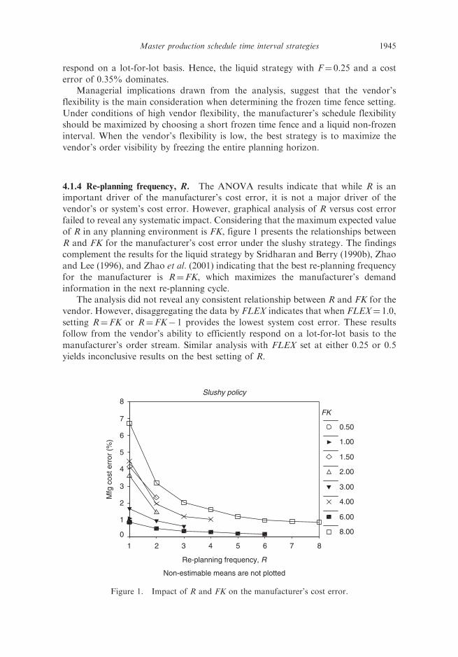
4.1.4 Re-planning frequency, R. The ANOVA results indicate that while R is animportant driver of the manufacturer’s cost error, it is not a major driver of the

vendor’s or system’s cost error. However, graphical analysis of R versus cost error

failed to reveal any systematic impact. Considering that the maximum expected value

of R in any planning environment is FK, figure 1 presents the relationships between

R and FK for the manufacturer’s cost error under the slushy strategy. The findings

complement the results for the liquid strategy by Sridharan and Berry (1990b), Zhao

and Lee (1996), and Zhao et al. (2001) indicating that the best re-planning frequency

for the manufacturer is R¼FK, which maximizes the manufacturer’s demand

information in the next re-planning cycle.The analysis did not reveal any consistent relationship between R and FK for the

vendor. However, disaggregating the data by FLEX indicates that when FLEX¼ 1.0,

setting R¼FK or R¼FK� 1 provides the lowest system cost error. These results

follow from the vendor’s ability to efficiently respond on a lot-for-lot basis to the

manufacturer’s order stream. Similar analysis with FLEX set at either 0.25 or 0.5

yields inconclusive results on the best setting of R.

Slushy policy

Non-estimable means are not plotted

Re-planning frequency, R

87654321

Mfg

cos

t err

or (

%)

8

7

6

5

4

3

2

1

0

FK

0.50

1.00

1.50

2.00

3.00

4.00

6.00

8.00

Figure 1. Impact of R and FK on the manufacturer’s cost error.


4.1.5 Natural Cycle (N ), Lumpiness (L), and Demand Range (DR). The ANOVAresults and the factor level mean values in table 1 indicate that these environmentalfactors have relatively lower impact on system cost error and consequently MPSperformance. While statistically significant at the 0.05 level, changes in N have littleimpact on cost error at the system level. However, it is noteworthy that increasing Nresults in decreasing cost error for the liquid policy, while the cost error increasesunder the slushy policy. Higher DR levels are associated with higher cost errors at themanufacturer, vendor and system. Results for L indicate a slight increase and thendecrease in cost error when moving to higher levels of demand lumpiness.

4.2 Impact of experimental factors on schedule instability

The research findings advance the MPS literature by providing comparative schedulenervousness measurements at the unit and order level for the manufacturer andvendor under the liquid and slushy policies. The analysis extends the literature’sscope from a single-stage to a two-stage supply chain context and provides insightsinto the relationship between MPS non-frozen interval policy and channel schedulestability. Table 4 summarizes the instability results by experimental factor.

The results of an ANOVA analysis indicate that all of the main effects and two-way interaction terms significantly influence the manufacturer’s quantity (MT1) andorder timing (MT2) instability at the 0.05 level except for FLEX and its interactionterms, which have no impact. In addition, K�DR for MT2 under the slushy policy isnot significant at the 0.05 level. The major drivers of both MT1 and MT2 scheduleinstability are F, K, R, N, and select interaction terms. F is the dominant factorinfluencing the manufacturer’s schedule instability. These general results for the

Table 4. Summary instability error results by factors (%).

Factor LevelLiquidMT1

LiquidMT2

LiquidVT1

LiquidVT2

SlushyMT1

SlushyMT2

SlushyVT1

SlushyVT2

Overall Average 17.85 12.98 23.70 11.53 9.15 4.31 53.36 36.03

FLEX 0.25 17.85 12.98 33.50 13.31 9.15 4.31 75.01 50.560.5 17.85 12.98 35.65 20.83 9.15 4.31 73.60 52.251.0 17.85 12.98 1.93 0.47 9.15 4.31 11.49 5.27

K 2 9.20 3.78 10.67 0.41 8.82 3.37 29.31 11.904 17.94 12.10 18.38 4.90 11.21 5.23 44.98 25.038 20.39 16.18 30.26 18.19 8.21 4.13 64.77 48.76

F 0.25 55.56 43.39 7.09 0.06 24.19 12.05 102.56 73.300.5 36.29 27.39 15.72 3.88 17.15 8.27 71.91 50.400.75 15.10 9.27 21.71 9.33 10.22 4.46 48.34 33.251.0 0.00 0.00 33.99 20.37 0.00 0.00 33.99 20.37

N 2 8.98 4.60 21.13 9.79 5.56 1.59 45.86 28.244 20.24 14.74 24.71 12.01 10.38 4.89 56.01 37.818 24.32 19.60 25.24 12.80 11.50 6.45 58.23 42.03

L 0.0 21.56 17.52 27.91 14.84 8.47 4.53 63.03 45.650.2 20.40 14.85 24.59 12.13 11.19 5.51 55.84 38.170.5 11.57 6.56 18.59 7.64 7.78 2.89 41.22 24.27

DR 50 18.03 13.71 24.58 12.35 8.02 4.00 55.05 37.54150 17.66 12.25 22.81 10.72 10.27 4.62 51.69 34.52


slushy strategy are consistent with earlier research findings for the manufacturerassuming a liquid strategy. As expected, due to decreased scheduling flexibility in thenon-frozen interval, the manufacturer’s schedule nervousness declines moving fromthe liquid to slushy strategy, where MT1 decreases from 17.85% to 9.15% and MT2declines from 12.98% to 4.31% (see table 4). It is worth noting that under the slushypolicy even though the timings of the current slushy orders remain constant, anadditional order may be inserted in the next planning cycle between the last slushyorder and the end of the planning horizon to reduce inventory costs (see theAppendix for an example). Hence, the manufacturer may experience order instabilityeven when implementing the slushy strategy.

The ANOVA analysis indicates that K, F, and R are the main drivers ofthe vendor’s schedule instability under the liquid policy, while K, R, and FLEXdrive the vendor’s schedule instability under the slushy policy. F is not a major driverof the vendor’s instability under the slushy strategy since all orders within theplanning horizon are passed to the vendor. Overall, moving from the liquid to theslushy strategy increases order quantity instability (VT1) from 23.7% to 53.36% andorder timing instability (VT2) from 11.53% to 36.03%. As expected, shifting to aslushy strategy extends the vendor’s order visibility to the full length of the planninghorizon and provides more opportunities for rescheduling.

4.2.1 Impact of K and FLEX�K. The findings for K under the liquid policy areintuitive, where increasing the length of the planning horizon promotes higher MT1,MT2, VT1, and VT2 schedule nervousness. An identical response pattern holds forVT1 and VT2 under the slushy policy. However, MT1 and MT2 for the slushy policyshow mixed results, where nervousness increases moving from K¼ 2 to K¼ 4 andthen decreases moving to K¼ 8. The lower nervousness at K¼ 8 appears related to areduction in the truncated planning horizon effect that is associated with the longerplanning horizon, which provides a more relatively efficient lot-size schedule early onthat is not as prone to change during later MPS updates.

Figure 2 presents MT1 and the interaction effects between FLEX�K for VT1under the slushy policy. As expected, at FLEX¼ 0.25 or 0.5 the vendor frequentlyreschedules in an attempt to lower costs. However, the results are counter-intuitive

Slushy policy

0

20

40

60

80

100

2 4 8

Planning horizon in natural cycles, K

Typ

e1 in

stab

ility

(%

)

Mfg (All FLEX)

Vend (FLEX=1)

Vend (FLEX=0.5)

Vend (FLEX=0.25)

Figure 2. Type 1 instability results for FLEX�K.


for FLEX¼ 1, where changes in K have little impact on the vendor’s instability.In this case, the vendor responds on a near lot-for-lot basis to the manufacturer’sorders with relatively low schedule nervousness. Similar results hold for FLEX�Kand VT2 under the slushy policy so they are not presented.

4.2.2 Impact of F and FLEX�F. Table 4 illustrates different schedule instabilityresponse patterns to changes in F for the manufacturer and vendor. The results forthe manufacturer under the liquid strategy are consistent with Sridharan et al. (1988),Sridharan and Berry (1990b), Zhao and Lee (1996) and Zhao et al. (2001), whereincreasing the frozen time interval decreases the manufacturer’s schedule nervous-ness. At F¼ 1.0, the entire planning horizon is frozen prohibiting rescheduling.Schedule freezing has an opposite impact on the vendor under the liquid policy,

where a longer frozen schedule interval increases the vendor’s planning horizon,opportunities to reschedule, and schedule nervousness. Similar relationships hold forMT2 and VT2 under the liquid policy.

Under the slushy policy, the manufacturer’s MT1 and MT2 schedule nervousnessalso decreases moving to a longer frozen interval, but the nervousness is considerablylower than under the liquid policy. The relationship between the vendor’s schedulenervousness and the length of the frozen interval are the opposite under the slushyand liquid policies for VT1 and VT2. Under the slushy policy, the vendor receivesplanning information beyond the frozen interval, which increases his schedulenervousness. However, increasing the length of the frozen interval converts themanufacturer’s slushy orders into frozen orders, which reduces the portion of ordersthat are subject to quantity change in the next MPS update. Hence, increasing thefrozen interval length reduces quantity nervousness for both the manufacturer and

vendor. At F¼ 1, all orders within the planning horizon are frozen and the schedulenervousness of the liquid and slushy policies are equal.

There is a strong interaction effect between FLEX and F for vendor scheduleinstability, where FLEX¼ 0.25 and 0.5 exhibit very high instability when comparedwith FLEX¼ 1. In addition, the rate of change in instability varies by FLEX.

4.2.3 Impact of R. Figure 3 illustrates the impact of changes in R on themanufacturer’s MT1 and vendor’s VT1 schedule instability at different frozeninterval lengths under the slushy policy. Both MT1 and VT1 schedule nervousness

decreases moving to higher levels of R for a specified FK. This is due to less frequentre-planning and higher quality schedules, due to increased demand visibility, that areless likely to be modified in subsequent MPS updates. When FK¼ 8, MT1¼ 0 for allvalues of R, since the entire planning horizon is frozen and not subject to change.The graphs also demonstrate that lower values of FK (i.e. shorter frozen intervals)provide more stable schedules for a specified value of R for both the manufacturerand vendor.

Similar response patterns are associated with MT2 and VT2 for the slushy policy,and the liquid policy’s instability metrics. However, when compared to the liquidstrategy, the slushy strategy results in a relatively more stable schedule for themanufacturer, while the vendor’s schedule is less stable.


4.2.4 Impact of N, DR and L. The environmental factors N, DR and L haverelatively little impact on schedule instability under both liquid and slushy policies.Longer natural cycle lengths are associated with higher manufacturer scheduleinstability under both liquid and slushy policies with the greater impact on the liquidpolicy. However, the impact of N on VT1 is not significant at the 0.05 level under theliquid policy. While significant at the 0.05 level for the slushy policy, N is not a majordriver of vendor schedule instability.

DR also exhibits a relatively small effect on the manufacturer’s and vendor’sschedule instability under the liquid and slushy policies. The impact of DR on VT1and VT2 is not significant at the 0.05 level for the liquid policy.

Manufacturer’s instability

Vendor’s instability

Replanning frequency, R87654321

Typ

e 1

inst

abili

ty (

%)

30

20

10

0

FK

0.50

1.00

1.50

2.00

3.00

4.00

6.00

8.00

0.50

1.00

1.50

2.00

3.00

4.00

6.00

8.00

Replanning frequency, R

87654321

Typ

e 1

inst

abili

ty (

%)

200

10

0

FK

Figure 3. Type 1 instability results by R and FK for the slushy policy.


Increases in demand lumpiness, L, result in lower schedule nervousness for the

manufacturer and vendor under the liquid policy. For the slushy policy, MT1 and

MT2 indicate a varying response to changes in L, while vendor instability is reduced

under more lumpy demand conditions. Overall, responses to changes in L are

relatively weak.

5. Conclusions and implications

It is well accepted that tighter integration of information and physical flows in supply

chains can yield significant productivity improvements. However, even though the

communication and information technologies are readily available, management has

been slow to capitalize on these new capabilities and move forward with system

improvement. This research attempts to accelerate the integration process by

clarifying the tradeoff between the alternative MPS and AOC design policies and

parameter settings that are available for managing manufacturer-vendor schedules

in two-stage make-to-order supply chains. As such it takes a much needed step in

expanding the research scope from an exclusive focus on the manufacturer’s

performance to consider both the manufacturer and vendor in terms of schedule cost

and stability performance. The research builds upon Sahin et al. (2004) seminal study

of MPS policy in two-stage make-to-order systems.Using computer simulation we evaluate the relative effectiveness of MPS liquid

and slushy non-frozen interval strategies in a rolling schedule environment. The

experimental design also considers the impact of other MPS design (planning

horizon length, frozen interval length, and re-planning frequency) and environmental

factors (channel flexibility, natural cycle length, demand lumpiness, and demand

range) on system performance. An important research finding is that vendor

flexibility and its interactions with MPS design factors are the most significant

drivers of system performance in two-stage supply chains. The natural order cycle

length, demand lumpiness, and demand range play a minor role in determining the

optimal MPS design parameter settings. Hence, the manager can focus on the

channel’s flexibility when setting MPS design parameters.In situations with high vendor flexibility, the optimal MPS policy calls for

settings that maximize the manufacturer’s scheduling flexibility but limit the advance

order information provided to the vendor. These settings include longer planning

horizons, short frozen intervals, re-planning at the end of the frozen schedule, and a

liquid non-frozen interval. However under low flexibility conditions, the optimal

MPS design curtails the manufacturer’s schedule flexibility so that advance orders

can be provided to the vendor. Here, policy settings favour a long planning horizon,

long frozen interval, and a slushy non-frozen interval. Selecting the incorrect non-

frozen interval policy can result in significant opportunity costs. For example, in a

scenario with FLEX¼ 0.25 and F¼ 0.25, following a slushy non-frozen interval

policy yields an 8.19% cost error versus a 52.08% cost error under a liquid policy.

Selecting the correct MPS parameter settings can yield substantial savings in a two-

stage supply chain.


The results also provide insights into the management of schedule stability. While

the slushy non-frozen interval strategy is typically viewed as a mechanism for

enhancing schedule stability, the research results indicate that it has a conflicting

impact on the manufacturer and vendor. Going from a liquid to a slushy strategy,

the manufacturer’s schedule nervousness decreases, while the vendor’s schedule

nervousness increases.Even though this research specifically addresses MPS policy in a serial two-

stage make-to-order supply chain, the general findings on MPS schedule cost and

instability hold regardless of the number of vendors or manufacturers in the two-

stage system. As such, it provides basic insights into the management of more

complex systems. For example, in a single manufacturer and multiple vendor

environment, the flexibility ratios and relative cost structures of the primary

vendors will be major determinants of the optimal MPS policy for the system.

Relatively high vendor flexibility ratios favour an MPS policy enhancing the

manufacturer’s MPS schedule flexibility, while low vendor flexibility ratios

promote an MPS policy enabling advance order commitments. In situations with

a variety of vendor flexibility ratios, the simulation procedures can be modified and

applied to gain insight into the best MPS policy design. Similar insights can be

developed for a single vendor and multiple manufacturer environment. We hope

this research encourages more additional research addressing MPS policy in more

complex systems.

Appendix. Impact of rolling planning horizons on slushy orders

The following example illustrates that under a slushy non-frozen interval policy, even

though the timings of slushy orders are fixed, new orders may be inserted within the

current planning horizon in the next planning cycle. Consider a 12-period planning

horizon, a 4-period frozen interval, and that re-planning occurs after each order is

executed. In the initial planning cycle, the manufacturer’s optimal order schedule is

to produce 190, 146 and 215 units in time periods 1, 5 and 9, respectively, as

illustrated below. The order in period 1 is frozen, whereas the orders in 5 and 9 are

slushy indicating that the order timings are fixed, but the quantities may vary in the

next planning cycle.The manufacturer’s second planning cycle covers periods 5–16, where the

order for 146 units remains unchanged and is converted from slushy to frozen

status. However, the order for 215 units in period 9 is reduced to 175 units in

the second planning cycle when the demand in period 12 is rescheduled for

supply from period 9 to a newly scheduled order in time 12, which covers the

demand for periods 12–16. Rescheduling the 40 units from period 9 to period 12

yields a $36 inventory cost saving (i.e. 40 units� 3 periods� $ 0.3 per item per

time period). However, scheduling the new order in period 12 instead of in

period 13 as might have been expected, increases the inventory cost for serving

periods 13, 14, 15 and 16 by $34.2 (i.e. 114 units� 1 period� $ 0.3 per item per

time period). Hence, the net savings for scheduling a setup in period 12 of the


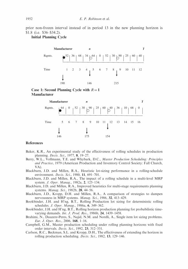
prior non-frozen interval instead of in period 13 in the new planning horizon is

$1.8 (i.e. $36–$34.2).Initial Planning Cycle

Manufacturer n T

Rqmts. 52 36 68 34 64 0 52 30 90 25 60 40

1 2 3 4 5 6 7 8 9 10 11 12Time

190 146 215

Case 1: Second Planning Cycle with R¼ 1

Manufacturer

Manufacturer n T

Rqmts.

Time

146 175 154

64 0 52 30 90 25 60 40 36 10 68 0

5 6 7 8 9 10 11 12 13 14 15 16

References

Baker, K.R., An experimental study of the effectiveness of rolling schedules in productionplanning. Decis. Sci., 1977, 8, 19–27.

Berry, W.L., Vollmann, T.E. and Whybark, D.C., Master Production Scheduling: Principlesand Practice, 1979 (American Production and Inventory Control Society: Fall Church,VA).

Blackburn, J.D. and Millen, R.A., Heuristic lot-sizing performance in a rolling-scheduleenvironment. Decis. Sci., 1980, 11, 691–701.

Blackburn, J.D. and Millen, R.A., The impact of a rolling schedule in a multi-level MRPsystem. J. Oper. Manag., 1982a, 2, 125–134.

Blackburn, J.D. and Millen, R.A., Improved heuristics for multi-stage requirements planningsystems. Manag. Sci., 1982b, 28, 44–56.

Blackburn, J.D., Kropp, D.H. and Millen, R.A., A comparison of strategies to dampennervousness in MRP systems. Manag. Sci., 1986, 32, 413–429.

Bookbinder, J.H. and H’ng, B.T., Rolling Production lot sizing for deterministic rollingschedules. J. Oper. Manag., 1986a, 6, 349–362.

Bookbinder, J.H. and H’ng, B.T., Rolling horizon production planning for probabilistic time-varying demands. Int. J. Prod. Res., 1986b, 24, 1439–1458.

Brahimi, N., Dauzere-Peres, S., Najid, N.M. and Nordli, A., Single item lot sizing problems.Eur. J. Oper. Res., 2006, 168, 1–16.

Campbell, G.M., Master production scheduling under rolling planning horizons with fixedorder intervals. Decis. Sci., 1992, 23, 312–331.

Carlson, R.C., Beckman, S.L. and Kropp, D.H., The effectiveness of extending the horizon inrolling production scheduling. Decis. Sci., 1982, 13, 129–146.


Carlson, R.C., Jucker, F.V. and Kropp, D.H., Less nervous MRP systems: a dynamiceconomic lot-sizing approach. Manag. Sci., 1979, 25, 754–761.

Chand, S., A note on dynamic lot sizing in a rolling-horizon environment. Decis. Sci., 1982,13, 113–119.

Chung, C. and Krajewski, L.J., Re-planning frequencies for master production schedules –notes and recommendations. Decis. Sci., 1986, 17, 263–273.

De Bodt, M.A. and Wassenhove, L.N.V., Cost increases due to demand uncertainty in MRPlot sizing. Decis. Sci., 1983, 14, 345–361.

Drexl, A. and Kimms, A., Lot sizing and scheduling-survey and extensions. Eur. J. Oper. Res.,1997, 99, 221–235.

Forrester, J.W., Industrial dynamics. Har. Bus. Rev., 1958, July-August, 37–66.Gilbert, S.M. and Ballou, R.H., Supply chain benefits from advanced customer commitments.

J. Oper. Manag., 1999, 18, 61–73.Kadipasaoglu, S.N. and Sridharan, V., Alternative approaches for reducing schedule

instability in multistage manufacturing under demand uncertainty. J. Oper. Manag.,1995, 13, 193–211.

Karimi, B., Fatemi Ghomi, S.M.T. and Wilson, J.M., The capacitated lot sizing problem:a review of models and algorithms. Omega, 2003, 31, 365–378.

Krajewski, L. and Wei, J.C., The value of production schedule integration in supply chains.Decis. Sci., 2001, 32, 601–634.

Kropp, D.H. and Carlson, R.C., A lot-sizing algorithm for reducing nervousness in MRPsystem. Manag. Sci., 1984, 30, 240–244.

Kropp, D.H., Carlson, R.C. and Jucker, J.V., Heuristic lot-sizing approaches for dealing withMRP system nervousness. Decis. Sci., 1983, 14, 156–169.

Lee, H.L., Padhamanabhan, V. and Whang, S., The bullwhip effect in supply chains. SloanManag. Rev., 1997, Spring, 93–102.

La Londe, B. and Ginter, J. The Ohio State University 2004 survey of career patterns inlogistics. Council of Supply Chain Management Professionals. Available online at:www.CSCMP.org/website/careers/patterns.asp. (Accessed 11 November 2004).

Lin, N. and Krajewski, L.J., A model for master production scheduling in uncertainenvironments. Decis. Sci., 1992, 23, 839–861.

Lin, N., Krajewski, L.J., Leong, G.K. and Benton, W.C., The effects of environmental factorson the design of master production scheduling systems. J. Oper. Manag., 1994, 11,367–384.

Lundin, R.A. and Morton, T.E., Planning horizons for the dynamic lot-size model: Zabel vs.protective procedures and computational results. Oper. Res., 1975, 23, 711–733.

Maes, J. and Van Wassenhove, L.N., Multi-item single level capacitated dynamic lotsizingheuristics: a computational comparison (Part II: Rolling horizon). IIE Trans., 1986,39, 124–129.

Ristroph, J.H., Simulation of ordering rules for single level MRP with a rolling horizon andno forecast error. Comp. Indust. Eng., 1990, 19, 155–159.

Russell, R.A. and Urban, T.L., Horizon extension for rolling production schedules: length andaccuracy requirements. Int. Journal of Prod. Econ., 1993, 29, 111–122.

Sahin, F. and Robinson, E.P., Flow coordination and information sharing in supply chains:review, implications and directions for future research. Decis. Sci., 2002, 33, 505–536.

Sahin, F., Robinson, E.P. and Gao, L.L. MPS policy and rolling schedules in a two-stagemake-to-order supply chain. Working paper, University of Tennessee, Knoxville, TN,2004.

Sahin, F. and Robinson, E.P., Information sharing and coordination in make-to-order supplychains. J. Oper. Manag., 2005, 23, 579–598.

Simpson, N.C., Multiple level production planning in rolling horizon assembly environments.Eur. J. Oper. Res., 1999, 114, 15–28.

Simpson, N.C., Questioning the relative virtues of dynamic lot sizing rules. Comp. Oper. Res.,2001, 28, 899–914.

Sridharan, V. and Berry, W.L., Freezing the master production schedule under demanduncertainty. Decis. Sci., 1990a, 21, 97–120.


Sridharan, V. and Berry, W.L., Master production scheduling, make-to-stock products:a framework for analysis. Int. J. Prod. Res., 1990b, 28, 541–558.

Sridharan, V. and LaForge, R.L., Freezing the master production schedule: implications forfill rate. Decis. Sci., 1994a, 25, 461–469.

Sridharan, V. and LaForge, R.L., A model to estimate service levels when a portion of themaster production schedule is frozen. Comp. Oper. Res., 1994b, 21, 477–486.

Sridharan, V., Berry, W.L. and Udayabhanu, V., Freezing the master production scheduleunder rolling planning horizons. Manag. Sci., 1987, 33, 1137–1149.

Sridharan, V., Berry, W.L. and Udayabhanu, V., Measuring master production schedulestability under rolling planning horizons. Decis. Sci., 1988, 19, 147–166.

Stadtler, H., Improved rolling schedules for the dynamic single-level lot-sizing problem.Manag. Sci., 2000, 2, 318–326.

Vollman, T.E., Berry, W.L. and Whybark, D.C., Manufacturing Planning and ControlSystems, 1998 (Irwin/McGraw Hill: NY).

Wagner, H.M. and Whitin, T.M., Dynamic version of the economic lot size model. Manag.Sci., 1958, 5, 89–96.

Wemmerlov, U. and Whybark, C.D., Lot-sizing under uncertainty in a rolling scheduleenvironment. Int. J. Prod. Res., 1984, 22, 467–484.

Yano, C.A. and Carlson, R.C., An analysis of scheduling policies in multi-echelon productionsystems. IIE Trans., 1985, 17, 370–377.

Yano, C.A. and Carlson, R.C., Interaction between frequency of rescheduling and the role ofsafety stock in MRP systems. Int. J. Prod. Res., 1987, 25, 221–232.

Yao, I. and Johnson, R.A., A new family of power transformations to improve normality orsymmetry. Biometrika, 2000, 87, 954–959.

Yeung, J.H.Y., Wong, W.C.K. and Ma, L., Parameters affecting the effectiveness of MRPsystems: A review. Int. J. Prod. Res., 1998, 36, 313–331.

Zhao, X. and Lam, K., Lot-sizing rules and freezing the master production schedule inmaterial requirements planning systems. Int. J. Prod. Econ., 1997, 53, 281–305.

Zhao, X. and Lee, T.S., Freezing the master production schedule in multilevel materialrequirements planning systems under deterministic demand. Prod. Plan. Cont., 1993, 7,144–161.

Zhao, X. and Lee, T.S., Freezing the master production schedule in multilevel materialrequirements planning system under deterministic demand. Prod. Plan. Cont., 1996, 7,144–161.

Zhao, X., Goodale, J.C. and Lee, T.S., Lot-sizing rules and freezing the MPS in materialrequirements planning systems under demand uncertainty. Int. J. Prod. Res., 1995, 33,2241–2276.

Zhao, X., Xie, J. and Jiang, Q., Lot-sizing rule and freezing the master production scheduleunder capacity constraint and deterministic demand. Prod. Oper. Manag., 2001, 10,45–67.

Zipkin, P.H., Foundations of Inventory Management, 2000 (Irwin/McGraw-Hill: New York).


Master production schedule time interval strategies in … · Master production schedule time...

Documents

Transcript of Master production schedule time interval strategies in … · Master production schedule time...