Master of Scien ani joupari

[Use 10-12 Point Font]

[Font Times New Roman]

[Thesis/Project Collaborative (same department) Title Page]

THE ELECTRICAL TRANSMISSION

SYSTEM OF A 345KV WITH 170 MILES MODEL

A Project

Presented to the faculty of the Department of Electrical and Electronic Engineering

California State University, Sacramento

Submitted in partial satisfaction of

the requirements for the degree of

MASTER OF SCIENCE

in

Electrical and Electronic Engineering

by

Farshad Tavatli

Babak Kaviani Joupari

SPRING

2013

ii

Sample Copyright page

[l]

© 2013[Year of graduation]

Farshad Tavatli


ALL RIGHTS RESERVED

[Thesis/Project Approval Page]

iii



A Project

by

Farshad Tavatli


Approved by:

__________________________________, Committee Chair Turan Gönen, Ph.D.

__________________________________, Second Reader Salah Yousif, Ph.D.

____________________________

Date

[Thesis/Project Format Approval Page]

iv

Student: Farshad Tavatli


I certify that these students have met the requirements for format contained in the

University format manual, and that this project is suitable for shelving in the Library and

credit is to be awarded for the project.

__________________________, Graduate Coordinator ___________________

B. Preetham. Kumar, Ph.D. r Date

Department of Electrical and Electronic Engineering

v

Abstract

of



by

Farshad Tavatli


A reliable and efficient transmission system benefits not only the power utility

companies, but the consumer as well. This report provides clarification to concepts and

calculations in the analysis of an electrical transmission system involving a 345KV with

170 miles of distance. The project will analyze the efficiency, voltage regulation, power

quality, power losses by comparing different sizes of cables.

A fundamental part of achieving a reliable transmission system is by considering all

necessary factors such as; careful design and complicated calculations “with help of

MATLAB”. Different compensator devices will be discussed and used in no load and full

load situations in this report in order to design an efficient transmission circuit.

_______________________, Committee Chair

Turan Gönen, Ph.D.

_______________________ Date

vi

DEDICATION

[Optional]

I dedicate this work to my parents and a great instructor “DR Gonen”.

vii

[This Table of Contents covers many possible headings. Pages are optional.

Use only the headings t

TABLE OF CONTENTS

Page

Dedication .................................................................................................................... vi

List of Tables .................................................................................................................x

List of Figures .............................................................................................................. xi

Chapter

1. INTRODUCTION ...................................................................................................1

2. LITERATURE SURVEY ........................................................................................2

2.1. Introduction ....................................................................................................2

2.2. Line Routing ..................................................................................................4

2.3. Ground Clearance ..........................................................................................4

2.4. Separation Between Conductors ....................................................................6

2.5. Insulation and Insulators ................................................................................6

2.6. Tower Structure .............................................................................................7

2.7. Sag and Tension .............................................................................................9

2.8. Thermal Ampacity .......................................................................................10

2.9. Line Parameters ...........................................................................................10

2.10. Inductance ..................................................................................................11

2.11. Capacitance ................................................................................................11

2.12. Transposition with Ground Wire ...............................................................12

viii

2.13. Long Line Model .......................................................................................12

2.14. Line Compensation ....................................................................................13

3. MATHEMATICAL MODEL ................................................................................14

3.1. Thermal Ampacity rating ....................................................................14

3.2. Series Impedance and shunt Admittance ............................................14

3.2.1. Series Impedance .................................................................................15

3.2.1a Self and Mutual Impedances with effects of Ground Wire .............17

3.2.2 Shunt Admittance..............................................................................23

3.3. Long Line Model .................................................................................29

3.4. ABCD Constants .................................................................................32

3.5. Voltage Regulation, Power Loss and Efficiency ................................32

3.6. Line Compensation .............................................................................33

3.6.1 Full Load Compensation ...................................................................34

3.6.2 No Load Compensation ....................................................................35

4. APPLICATION OF THE MATHEMATICAL MODEL ......................................39

4.1. Introduction ..........................................................................................39

4.2. Thermal Ampacity Rating...................................................................41

4.3. Line Characteristics and ABCD Constants ..........................................42

4.3.1 Series Impedance ..............................................................................43

4.3.2 Shunt Admittance..............................................................................46

4.3.3 ABCD Constants ...............................................................................50

ix

4.4. Uncompensated Line ...........................................................................51

4.4.1 Full Load ...........................................................................................52

4.4.2 No Load ............................................................................................53

4.4.3 Voltage Regulation, Power Loss and Efficiency ..............................53

4.4.4 MATLAB ..........................................................................................54

4.5. Compensation ......................................................................................55

4.5.1 Full Load Compensation ...................................................................55

4.5.2 No Load Compensation ....................................................................56

5. SUMMARY ...........................................................................................................60

Appendix A. Overhead Ground Wire Characteristics .................................................62

Appendix B. ACRS Table............................................................................................64

Appendix C. Wire Compensation of Uncompensated Line data .................................65

Appendix D. MATLAB Code of Uncompensated Line ..............................................67

Appendix E. MATLAB Code, Full Load Compensation ............................................71

Appendix F. MATLAB Code, No Load Compensation ..............................................76

Bibliography ................................................................................................................79

x

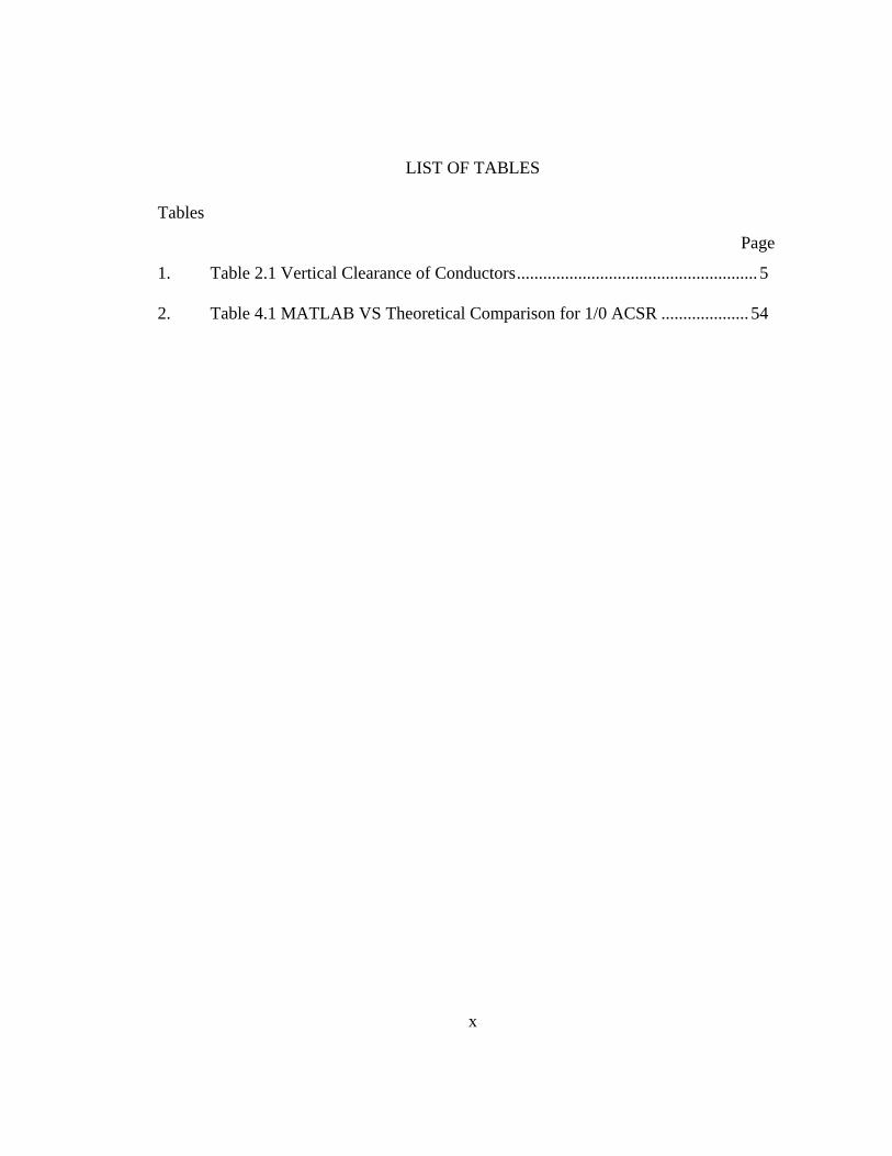
LIST OF TABLES

Tables

Page

1. Table 2.1 Vertical Clearance of Conductors ....................................................... 5

2. Table 4.1 MATLAB VS Theoretical Comparison for 1/0 ACSR .................... 54

xi

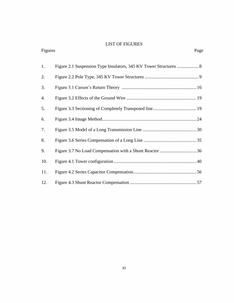
LIST OF FIGURES

Figures Page

1. Figure 2.1 Suspension Type Insulators, 345 KV Tower Structures ................... 8

2. Figure 2.2 Pole Type, 345 KV Tower Structures ............................................... 9

3. Figure 3.1 Carson’s Return Theory ................................................................. 16

4. Figure 3.2 Effects of the Ground Wire ............................................................. 19

5. Figure 3.3 Sectioning of Completely Transposed line ...................................... 19

6. Figure 3.4 Image Method .................................................................................. 24

7. Figure 3.5 Model of a Long Transmission Line ............................................... 30

8. Figure 3.6 Series Compensation of a Long Line .............................................. 35

9. Figure 3.7 No Load Compensation with a Shunt Reactor ................................ 36

10. Figure 4.1 Tower configuration ........................................................................ 40

11. Figure 4.2 Series Capacitor Compensation ....................................................... 56

12. Figure 4.3 Shunt Reactor Compensation .......................................................... 57

1

Chapter 1

INTRODUCTION

The purpose of this project is to find a means of choosing a line based on its voltage

regulation, power loss, and efficiency. A voltage regulation between 3% and 5% will be

ideal, while minimizing power loss and maximizing efficiency. Since ACSR (Aluminum

Conductor cable Steel Reinforced) conductors are widespread used for transmission line

design, therefore in this project we will be using ACSR as well. A line will be selected in

the beginning just to show the hand calculations then MATLAB will be used to execute

the same calculations but for different line sizes. A static receiving end load with a

lagging power factor will be analyzed for a 170 miles long line at 345kv. An overhead

ground wire will be used for lightning protection and will be taken into consideration

when computing the long line parameters. The tower configuration to be used will be

arbitrarily selected as well as the overhead ground wire type. The computational method

is the most significant portion of this analysis; therefore all structural and mechanical

aspects will be ignored. From this analysis the data can then be used for an economic

analysis which would involve line initial cost, construction, maintenance, operation,

efficiency, compensation Vars, and reliability.[1]

Equation Chapter (Next) Section 1

Equation Chapter (Next) Section 1

2

Chapter 2

LITERATURE SURVEY

2.1 INTRODUCTION

Designing Transmission lines is definitely not a simple task. There are so many

considerations that have to be factored in to make an efficient and worth building

transmission line. In addition, there are certain regulations that have to be met for the

safety and wellbeing not just for the people but also for the environment. Such

considerations are as following; Line Routing, Cost Estimating, Station Interfacing,

Right-of Way Acquisition, Structure Design, Sag and Tension, Conductor Analysis,

clearances, strengths and loading, and many more which we cannot explain all of them in

this research. On top of all regulations also have to be considered from the National

Electric Code (NEC) and the National Electric Safety Code (NESC). The noticeable

difference between the two is that the NESC is not intended as a design specification or

an instruction manual. The NEC covers the proper installation guidelines of electric

conductors on buildings or structures that need to be considered to protect the people and

property from hazards that occur from the usage of electricity in building and structures.

The NESC addresses the practical safety and the basic provisions that are considered

essential for the safety of the workers and the public. [2]

Transmission lines were not always generated by alternating current (AC). In fact, Direct

Current (DC) was first used as generation in 1882. However, it was quickly found

3

inefficient because voltage could not be increased for a long distance. The classes of

loads are variable so it required different voltages and would result in different generators

and circuits. Nikola Tesla proposed the use of alternating current which allowed efficient

generation. With the use of rotary converters, an electrical machine used to convert one

form of electrical power to another, networks connecting different generating plants with

loads having different frequencies could be connected. Also, AC could be converted to

DC with the use of rotary converter to be served to the loads that required DC. By

permitting multiple interconnections between several generating plants, electricity

production was more efficient resulting in the decrease in cost. Reliability immensely

improved and also resulted in lower production cost. [2]

AC Power can be transported by two ways. One is overhead transmission and the other is

underground transmission. In overhead transmission, the electrical conductors are not

covered by insulation. The conductors that are used are mainly Aluminum Conductor

Steel Reinforced (ACSR). They are used as bare overhead transmission cable or primary

and secondary distribution cable. The underground transmission is mainly used in

densely congested areas and also where there are natural obstacles that do not permit the

use of overhead transmission. The use of underground transmission is a more expensive

option, actually about two to four times the cost of an overhead line.

4

2.2 LINE ROUTING

One major consideration that has to be taken into account for transmission line design is

the route of the lines. Where will these lines carrying so much voltage go? Selecting a

route may not be an easy task. There are many considerations that need to be thought

taken. For instance, there are physical (highways, railroads, other transmission lines),

biological (wetlands, wildlife, woodlands), or other (federal, state controlled lands). Not

only do these locations have to be examined, the cost of clearing, ease of maintaining,

and the effect of the line may have on the environment. After the route has been selected,

the surveyors conduct a field examination and prepare a universal drawing for the whole

route. Also, there are many permits and authorizations that need to be obtained. For

instance, federal permits or licenses are required, the use of private property, permit from

state/county/city, permission of utility. There are others that need to be obtained but for

the limited space of this report, they shall not be listed. [1]

2.3 GROUND CLEARANCE

This is where the NESC come into play. There has to be enough clearances under the line

so it will not pose any danger to anything underneath the line. Such clearances to

consider are clearances over water surface, ground, roadways, or rails. The NESC

specifies all of these under different types of nominal line voltages. For example, for a

230 KV line, there has to be at least 32.9 ft of clearance for track rails, 24.9 ft for roads

and streets, and 20.9 for spaces and ways for accessible to pedestrians only. Not only is

there vertical clearance, there is also horizontal clearance in order to provide more

5

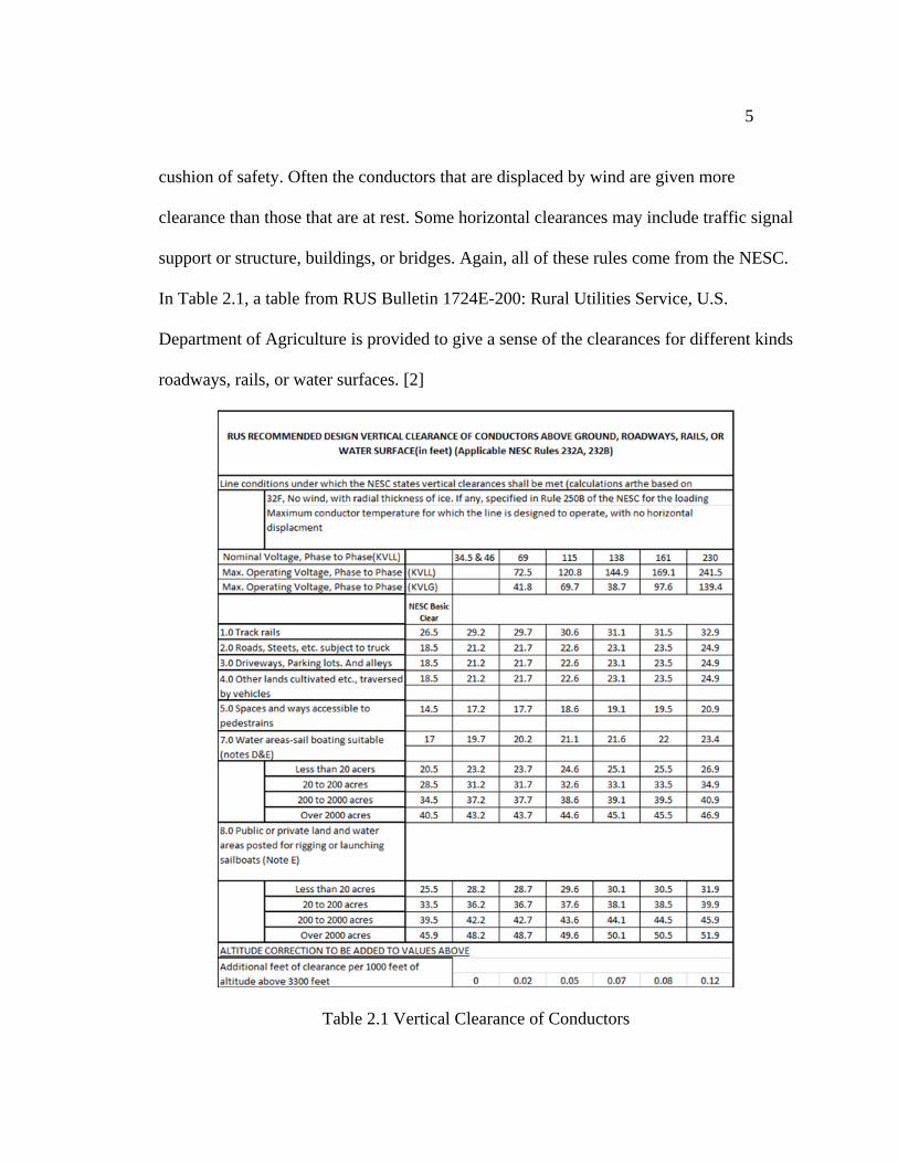
cushion of safety. Often the conductors that are displaced by wind are given more

clearance than those that are at rest. Some horizontal clearances may include traffic signal

support or structure, buildings, or bridges. Again, all of these rules come from the NESC.

In Table 2.1, a table from RUS Bulletin 1724E-200: Rural Utilities Service, U.S.

Department of Agriculture is provided to give a sense of the clearances for different kinds

roadways, rails, or water surfaces. [2]

Table 2.1 Vertical Clearance of Conductors

6

2.4 SEPARATION BETWEEN CONDUCTORS

Conductors are always assumed to move. On that note, there should always be a

minimum separation between each phase of the conductors. If insulators are free to

swing, that means the conductors are also going to swing since the conductor hangs from

the insulator. The separation between the lines will depend on the spans and sags of the

lines as well as how structures match up with another. The standard separation value

should be on a worst case analysis.

Galloping or “dancing” occurs where the conductors move with very high

amplitudes. This is bad because it can cause contact between phase conductors or the

overhead ground wire, which will cause a major electrical outage. Also, the conductor

themselves may break due to the intense stress, or maybe the structure or towers

themselves may have possible damage. Galloping is caused by stable wind blowing over

the conductors covered by a layer of ice deposited from the freezing rain. There are

measures to take to reduce the possible contact between the conductor phases that are

caused by galloping. For instance, shorter spans, which are the distance from one tower

to another, or increased, phase separation between the conductors. [1]

2.5 INSULATION AND INSULATORS

Insulators are objects that have to be considered when designing transmission lines. An

object made of a material like glass, porcelain or composite polymer that is a poor

conductor of electricity. All of the materials for insulators are handled with epoxy resins,

which acts like reinforcement glue for the materials of the insulators. Insulators are used

7

to attach conductors to the transmission structure and to prevent a short circuit from

happening between the conductor and the structure. For this design suspension type

insulators will be used, since they are used for very high voltage systems is not a practical

or safe to use other types of insulators. Suspension type insulators are usually made of

porcelain that can be stacked in a string and hangs from a cross arm on a tower or pole

that supports the line conductor. Fig 2.2 illustrates suspension type insulators hanging

from a steel lattice tower.

There are also pin-typed insulators to secure the conductor to the insulator. Another type

of insulator is the strain insulator. These types of insulators are used on when the line is

dead-ended. It provides adequate mechanical strength to counterbalance the forces due to

the tension of the conductors and as well as provide insulation. [1][3]

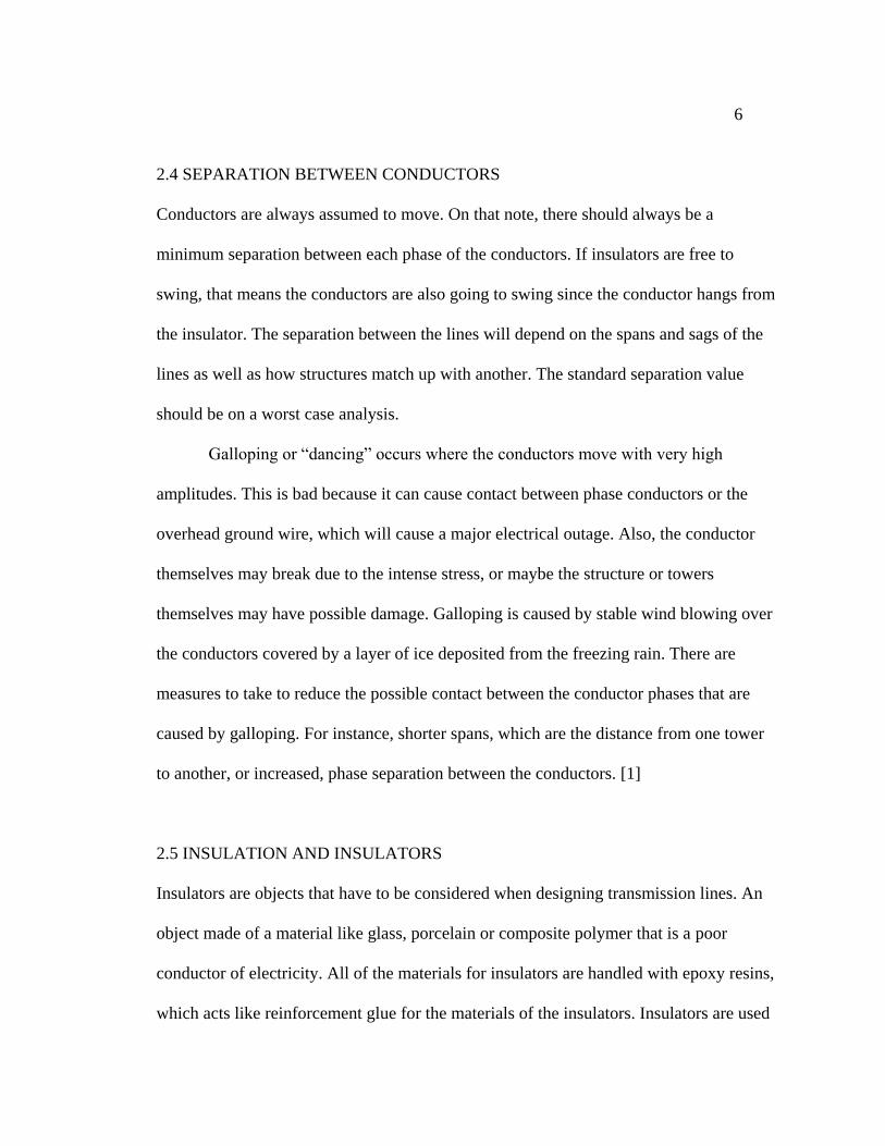
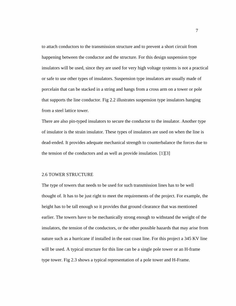
2.6 TOWER STRUCTURE

The type of towers that needs to be used for such transmission lines has to be well

thought of. It has to be just right to meet the requirements of the project. For example, the

height has to be tall enough so it provides that ground clearance that was mentioned

earlier. The towers have to be mechanically strong enough to withstand the weight of the

insulators, the tension of the conductors, or the other possible hazards that may arise from

nature such as a hurricane if installed in the east coast line. For this project a 345 KV line

will be used. A typical structure for this line can be a single pole tower or an H-frame

type tower. Fig 2.3 shows a typical representation of a pole tower and H-Frame.

8

Figure 2.1 Suspension Type Insulators, 345 KV Tower Structure

9

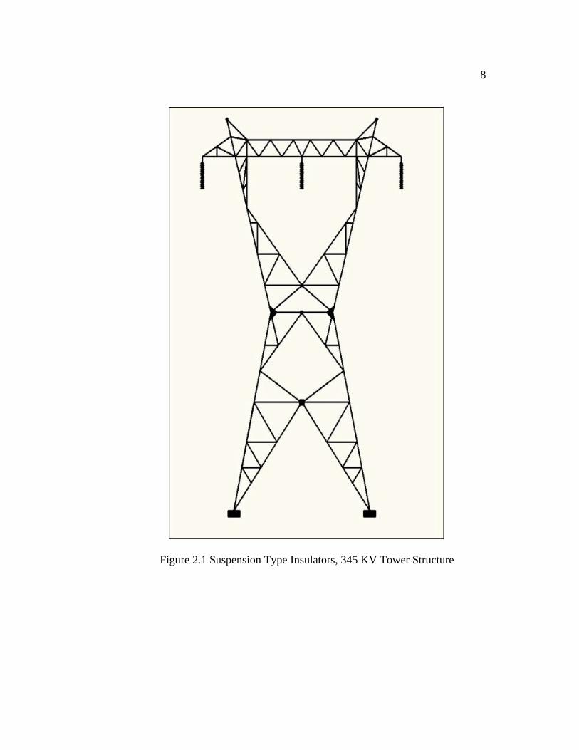
Figure 2.2 Pole Type, 345 KV Tower Structure

Another type of tower structure is the steel lattice tower. These towers are for extra high

voltages. [1] [3]

2.7 SAG AND TENSION

In transmission lines, the behaviors of the hanging conductors are a key variable for the

design. For instance, some factors that will contribute to the sag are the temperature of

the environment, temperature of the conductor itself, the current running through the line,

and the weight of the conductor. These are just the simple factors that will depend on

10

how much the line will sag at each span (distance between each tower). In addition, all

have to be met within the desired NESC regulations. Tension is correlated with the sag.

Tension should not be too high or too low because that will also contribute to the sag.

Having a higher tension will increase the sag and vice versa.

2.8 THERMAL AMPACITY

Transmission lines have the capability of transmitting power, which is limited to the

thermal loading and stability limits. The temperature of the conductor reflects the

thermal loading limit of the line and the real power loss of the line is increased as the

temperature of the conductors rise. The thermal limit is specified to be at 75% of the

current carrying capacity given for a conductor at a temperature of 50° Celsius. This

temperature of 50° Celsius is based on a 25° Celsius air temperature with a 25° Celsius

rise in conductor temperature. In order to find the current carrying capacity, the power of

the line and the rated phase voltage of the selected line should be known. [3]

2.9 LINE PARAMETERS

In modeling a transmission line, the resistance, inductance and capacitance of the line

must be taken into consideration. These parameters will be used to find the series

impedance and shunt admittance of the line which will then be used to find the ABCD

constants that will relate the sending and receiving end of the line.

11

2.10 INDUCTANCE

The inductance of a conductor is caused by the current being carried by the conductor

and the magnetic field around the conductor. As the current changes, the flux changes

and a voltage is induced in the circuit. There is also inductance inside a conductor. For

this design, the skin effect, which is the tendency of the alternating current to dispense

itself into the surface of the conductor making the current greater at the surface than the

center, will be neglected and assume that there is uniform current density throughout the

conductor cross section. The total inductance of the line will be the sum of the internal

and external flux linkages of the conductor.

2.11 CAPACITANCE

The capacitance of a transmission line is determined by the potential differences between

the conductors. The capacitance is a ratio of the charge of the conductor to the potential

difference of the conductor. The bigger the potential difference between the conductors

will result in smaller capacitance of the line and it is conversely the same if the potential

difference was very small. In contrast with the inductor, capacitance is associated with

electric field. The charge on a conductor increases the electric field with radial flux lines.

Overall the total capacitance of the line in a three phase system is the sum of the self and

mutual capacitances.

12

2.12 TRANSPOSITION WITH GROUND WIRE

The transposition of a line allows for a line to have approximately equal parameters. This

allows for the line to be modeled by one single phase to neutral line, with the addition of

an Overhead Ground Wire. Since all three phases occupy the same position for the same

amount of time,

2.13 LONG LINE MODEL

For a long transmission line the magnitude of the voltage over the entire line is not

constant. For relatively small loads or an open circuit condition, the voltage increases

from the sending end to the receiving end. For larger loads or the short circuit condition,

the voltage decreases depending on the amount of load. These increases and decreases in

the line voltage are unwanted. A decrease in voltage means an increase in current. This

would increase the power losses in the line and decrease the lines loading capability. For

the open circuit or small load situation, an increase in voltage would cause the line to be

more prone to arcing.

There are many ways of compensating a line. In this report, full load and no load

compensation will be our primary focus. The open circuit situation has its voltage

compensated with a single shunt reactor applied at the receiving end. For the full load

situation, compensation is achieved with the placement of a series capacitor in the middle

of the transmission line. Again, the idea is to understand how the line can be

compensated for the worst case scenarios up to but not including the thermal ampacity of

the line.

13

2.14 LINE COMPENSATION

For a long transmission line the magnitude of the voltage over the entire line is not

constant. For relatively small loads or an open circuit condition, the voltage increases

from the sending end to the receiving end. For larger loads or the short circuit condition,

the voltage decreases depending on the amount of load. These increases and decreases in

the line voltage are unwanted. A decrease in voltage means an increase in current. This

would increase the power losses in the line and decrease the lines loading capability. For

the open circuit or small load situation, an increase in voltage would cause the line to be

more prone to arcing.

There are many ways of compensating a line. In this report, full load and no load

compensation will be our primary focus. The open circuit situation has its voltage

compensated with a single shunt reactor applied at the receiving end. For the full load

situation, compensation is achieved with the placement of a series capacitor in the

middle of the transmission line. Again, the idea is to understand how the line can be

compensated for the worst case scenarios up to but not including the thermal ampacity

of the line.

14

Chapter 3

MATHEMATICAL MODEL

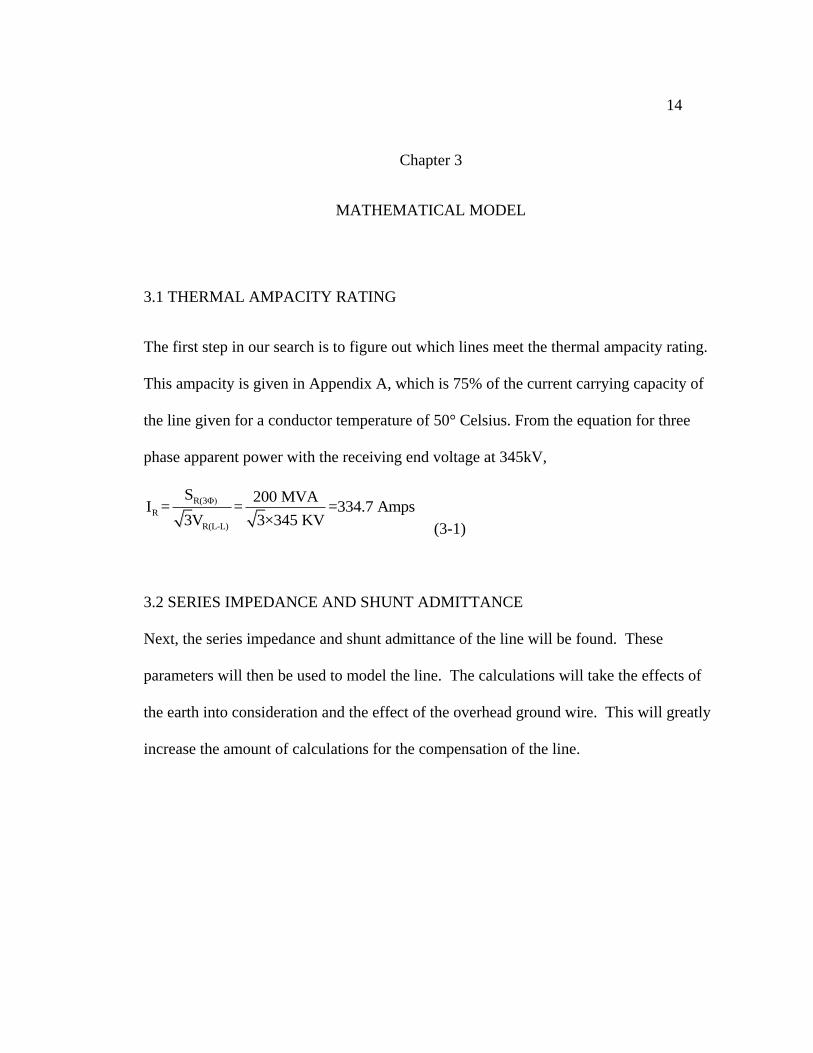
3.1 THERMAL AMPACITY RATING

The first step in our search is to figure out which lines meet the thermal ampacity rating.

This ampacity is given in Appendix A, which is 75% of the current carrying capacity of

the line given for a conductor temperature of 50° Celsius. From the equation for three

phase apparent power with the receiving end voltage at 345kV,

R(3Φ)

R

R(L-L)

S 200 MVAI = = =334.7 Amps

3V 3×345 KV (3-1)

3.2 SERIES IMPEDANCE AND SHUNT ADMITTANCE

Next, the series impedance and shunt admittance of the line will be found. These

parameters will then be used to model the line. The calculations will take the effects of

the earth into consideration and the effect of the overhead ground wire. This will greatly

increase the amount of calculations for the compensation of the line.

15

3.2.1 SERIES IMPEDANCE

Series impedance exists on a line due to inductance and resistance. The current through

any conductor develops a magnetic field of proportional magnitude. The energy is then

stored in the magnetic field, and there is opposition to change in currents, meaning the

current through the inductors cannot change rapidly. Each conductor in a three phase

system develops a magnetic field as it carries charging currents for the capacitance

between the wires. Since there is always a return current path present, the magnetic field

created by a changing magnetic field current in the circuit itself induces a voltage in the

same circuit. Since the system is three phase, there will be induced voltage on a line

from a current adjacent to another line.

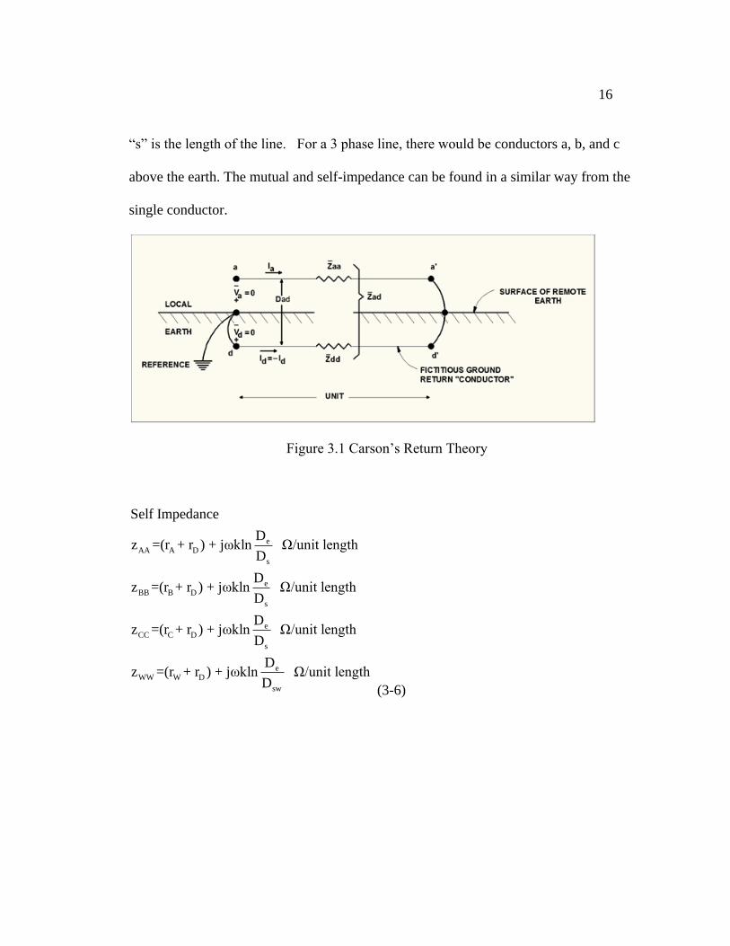
From Carson’s Earth Return Theory, there flows a current through a given conductor "a"

above the earth and another given conductor "d" in the earth.

By using Carson’s line formula, [5]

A A DD AD AV =(z +z 2z )I V/unit length. (3-2)

Also knowing that,

AA A DD ADz =(z +z 2z ) (3-3)

The self-impedance of conductor a can be established, by using Newman’s formula

AA Az =r + jωL. (3-4)

AA A

SA

2sz =r + jωkln Ω/unit length

D (3-5)

16

“s” is the length of the line. For a 3 phase line, there would be conductors a, b, and c

above the earth. The mutual and self-impedance can be found in a similar way from the

single conductor.

Figure 3.1 Carson’s Return Theory

eAA A D

s

eBB B D

s

eCC C D

s

eWW W D

sw

Self Impedance

Dz =(r + r ) + jωkln Ω/unit length

D


D


D


D(3-6)

17

eAB BA D

AB

eBC CB D

BC

eCA AC D

CA

eAW WA D

AW

BW WB D

Mutual Impedance

Dz = z = r + jωkln Ω/unit length

D


D

Dz =z = r + jωkln Ω/unit length

D


D

z = z = r + jωk e

BW

eCW WC D

CW

Dln Ω/unit length

D

Dz =z =r +jωkln Ω/unit length

D (3-7)

3.2.1a SELF AND MUTUAL IMPEDANCES WITH EFFECTS OF GROUND

WIRE

The self and mutual impedances are a result of the self and mutual inductance.

The impedance is the sum of the inductance and the resistance. A ground wire “W” will

be added to our 3 phase system.

18

-3

e

S SW

AB BC CA AW BW CW

-3

D

where:

ω= 2πf @ f = 60 hz

k= 0.3219x10 mile

ρD = 2160 = 2790 ft. @ ρ=100 Ω×m for Avg. soil

f

D , D = GMR of each conductor

D , D , D , D , D & D = distance between conductors

r = 1.588x10 f Ω/mil

A B C

W

e

r = r = r = resistance of lines Ω/mile

r = resistance of ground wire Ω/mile

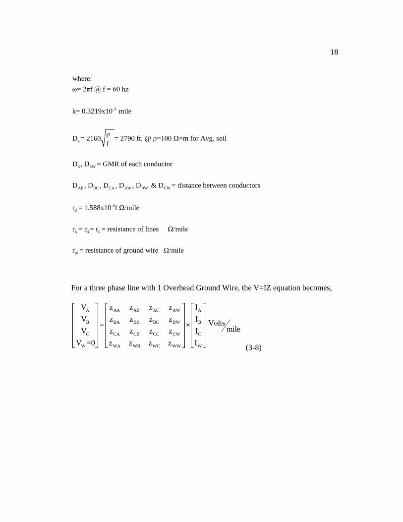
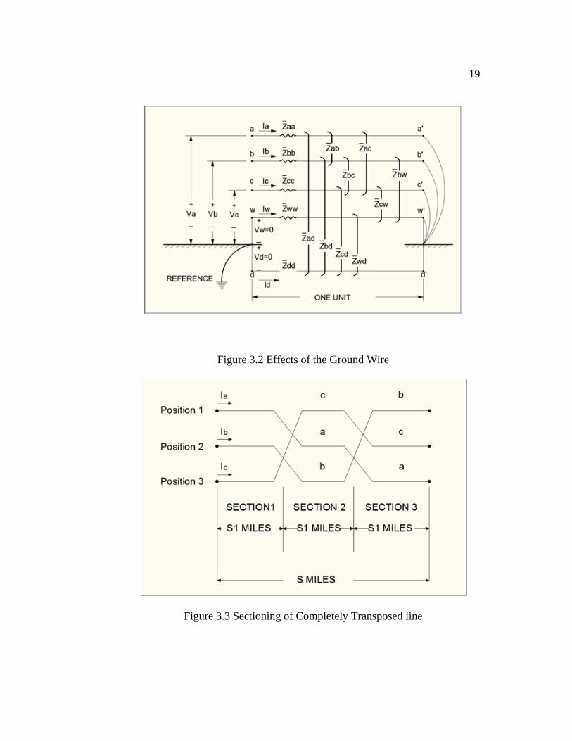
For a three phase line with 1 Overhead Ground Wire, the V=IZ equation becomes,

A AA AB AC AW A

B BA BB BC BW B

C CA CB CC CW C

W WA WB WC WW W

V z z z z I

V z z z z IVolts= ×

mileV z z z z I

V =0 z z z z I (3-8)

19

Figure 3.2 Effects of the Ground Wire

Figure 3.3 Sectioning of Completely Transposed line

20

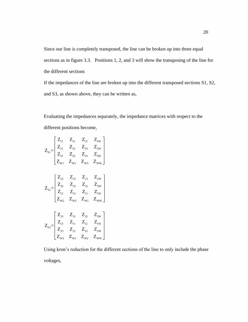
Since our line is completely transposed, the line can be broken up into three equal

sections as in figure 3.3. Positions 1, 2, and 3 will show the transposing of the line for

the different sections

If the impedances of the line are broken up into the different transposed sections S1, S2,

and S3, as shown above, they can be written as,

Evaluating the impedances separately, the impedance matrices with respect to the

different positions become,

11 12 13 1W

21 22 23 2W

S1

31 32 33 3W

W1 W2 W3 WW

22 23 21 2W

32 33 31 3W

S2

12 13 11 1W

W2 W3 W1 WW

33 31 32 3W

13 11 12 1W

S3

23 21 22 2W

W3 W1 W2 WW

Z Z Z Z

Z Z Z ZZ =

Z Z Z Z

Z Z Z Z

Z Z Z Z

Z Z Z ZZ =

Z Z Z Z

Z Z Z Z

Z Z Z Z

Z Z Z ZZ =

Z Z Z Z

Z Z Z Z

Using kron’s reduction for the different sections of the line to only include the phase

voltages,

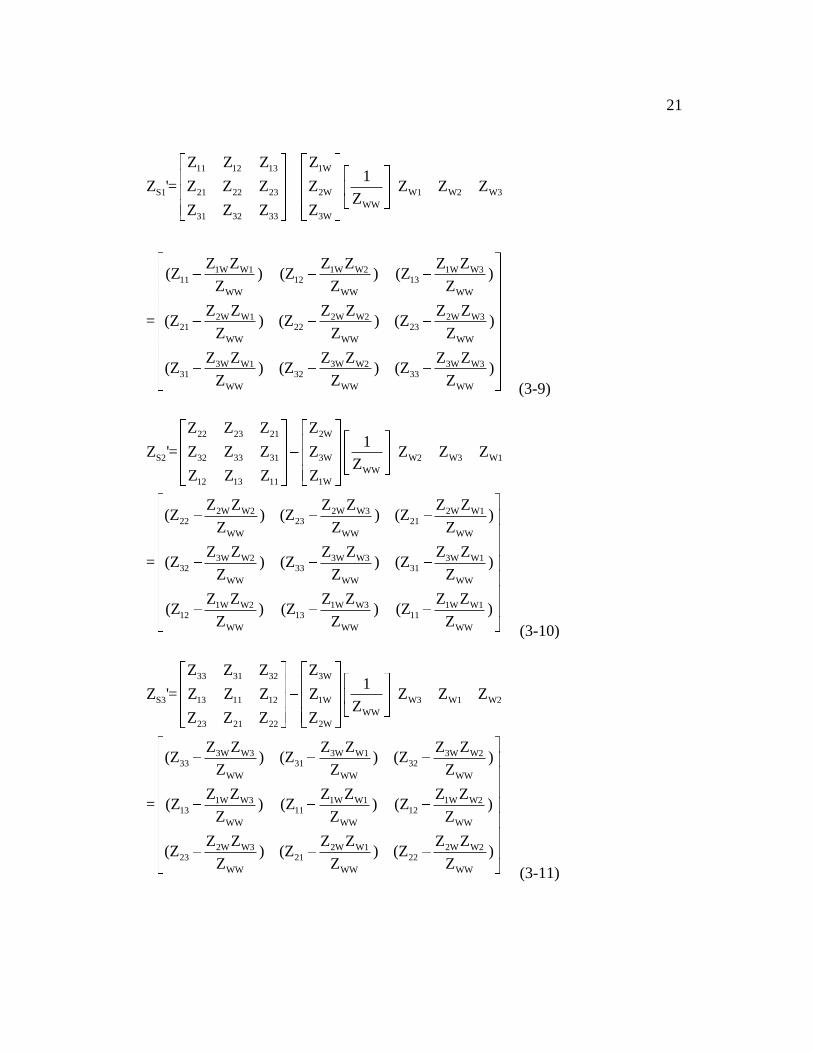
21

11 12 13 1W

S1 21 22 23 2W W1 W2 W3

WW

31 32 33 3W

1W W1 1W W2 1W W311 12 13

WW WW WW

2W W1 2W W2 2W W321 22 23

WW WW WW

3W W1 3W W231 32

WW W

Z Z Z Z1

Z '= Z Z Z Z Z Z ZZ

Z Z Z Z

Z Z Z Z Z Z(Z ) (Z ) (Z )

Z Z Z

Z Z Z Z Z Z= (Z ) (Z ) (Z )

Z Z Z

Z Z Z Z(Z ) (Z

Z Z

3W W333

W WW

Z Z) (Z )

Z (3-9)

22 23 21 2W

S2 32 33 31 3W W2 W3 W1

WW

12 13 11 1W

2W W2 2W W3 2W W122 23 21

WW WW WW

3W W2 3W W3 3W W132 33 31

WW WW WW

1W W2 1W W312 13

WW W

Z Z Z Z1

Z '= Z Z Z Z Z Z ZZ

Z Z Z Z

Z Z Z Z Z Z(Z ) (Z ) (Z )

Z Z Z

Z Z Z Z Z Z= (Z ) (Z ) (Z )

Z Z Z

Z Z Z Z(Z ) (Z

Z Z

1W W111

W WW

Z Z) (Z )

Z (3-10)

33 31 32 3W

S3 13 11 12 1W W3 W1 W2

WW

23 21 22 2W

3W W3 3W W1 3W W233 31 32

WW WW WW

1W W3 1W W1 1W W213 11 12

WW WW WW

2W W3 2W W123 21

WW W

Z Z Z Z1

Z '= Z Z Z Z Z Z ZZ

Z Z Z Z

Z Z Z Z Z Z(Z ) (Z ) (Z )

Z Z Z

Z Z Z Z Z Z= (Z ) (Z ) (Z )

Z Z Z

Z Z Z Z(Z ) (Z

Z Z

2W W222

W WW

Z Z) (Z )

Z (3-11)

22

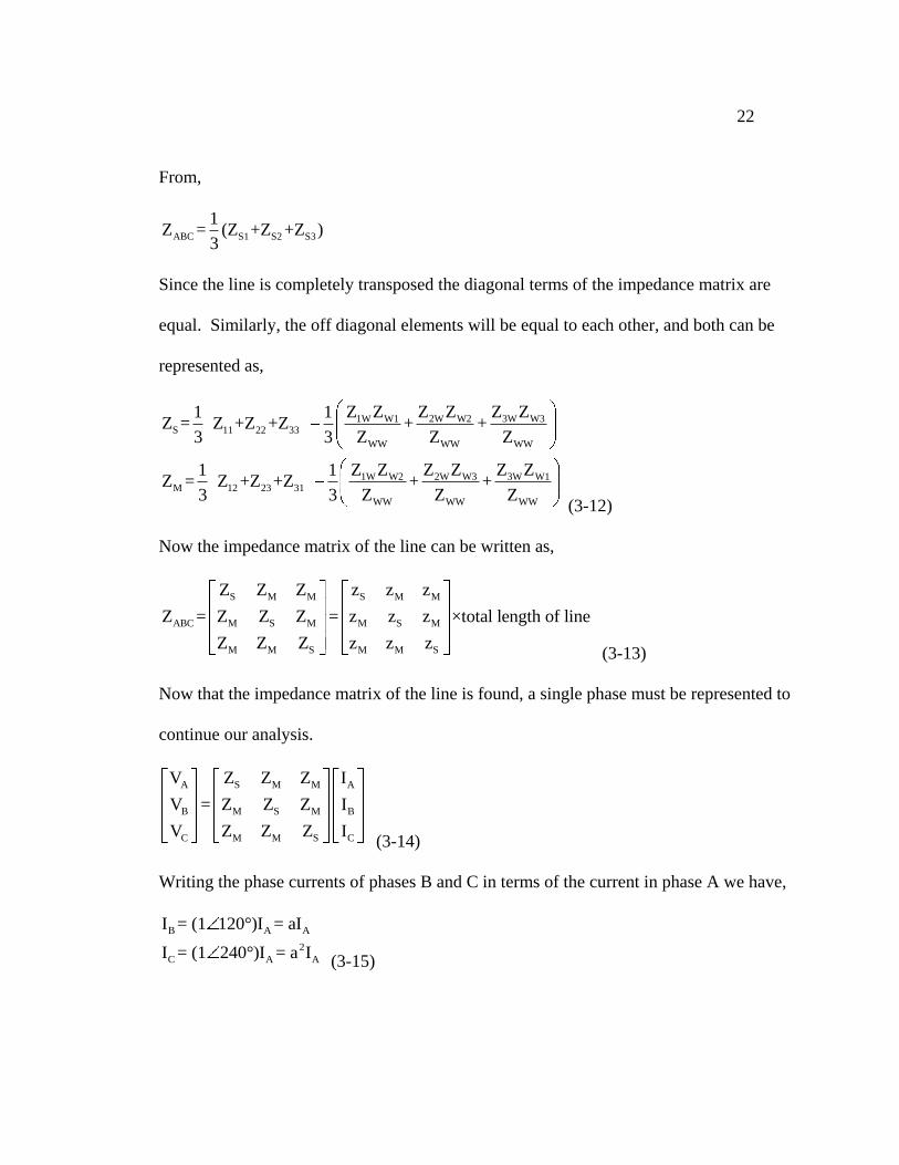
From,

ABC S1 S2 S3

1Z = (Z +Z +Z )

3

Since the line is completely transposed the diagonal terms of the impedance matrix are

equal. Similarly, the off diagonal elements will be equal to each other, and both can be

represented as,

1W W1 2W W2 3W W3S 11 22 33

WW WW WW

1W W2 2W W3 3W W1M 12 23 31

WW WW WW

Z Z Z Z Z Z1 1Z = Z +Z +Z + +

3 3 Z Z Z

Z Z Z Z Z Z1 1Z = Z +Z +Z + +

3 3 Z Z Z (3-12)

Now the impedance matrix of the line can be written as,

S M M S M M

ABC M S M M S M

M M S M M S

Z Z Z z z z

Z = Z Z Z = z z z ×total length of line

Z Z Z z z z (3-13)

Now that the impedance matrix of the line is found, a single phase must be represented to

continue our analysis.

A S M M A

B M S M B

C M M S C

V Z Z Z I

V = Z Z Z I

V Z Z Z I (3-14)

Writing the phase currents of phases B and C in terms of the current in phase A we have,

B A A

2

C A A

I = (1 120°)I = aI

I = (1 240°)I = a I (3-15)

23

A S M M A

B M S M A

2

C M M S A

V Z Z Z I

V = Z Z Z aI

V Z Z Z a I (3-16)

Using only phase A to represent the series impedance of the line,

2

A S A M A M

2

A S M

A S M

V=I Z +aI Z +a I Z

=I Z + a+a Z

=I Z -Z (3-17)

Therefore, the series impedance of the line can be found as,

S M

1W W1 2W W2 3W W3 1W W2 2W W3 3W W111 12 23 31

WW WW WW WW WW WW

Z=Z Z

Z Z Z Z Z Z Z Z Z Z Z Z1 1 1=Z + + Z +Z +Z + +

3 Z Z Z 3 3 Z Z Z (3-18)

3.2.2 SHUNT ADMITTANCE

The shunt admittance of a line is of the form Y = g +jωC. Where g is the

conductance of the line and is considered negligible. Therefore Y = jωC. For a 3 phase

line, the capacitance is found first by its potential coefficients where,

1

volts

and

unit lengthFarad

qV Pq

C

P C

24

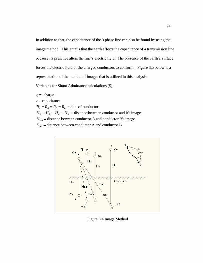
In addition to that, the capacitance of the 3 phase line can also be found by using the

image method. This entails that the earth affects the capacitance of a transmission line

because its presence alters the line’s electric field. The presence of the earth’s surface

forces the electric field of the charged conductors to conform. Figure 3.5 below is a

representation of the method of images that is utilized in this analysis.

Variables for Shunt Admittance calculations [5]

charge

capacitance

radius of conductor

distance between conductor and it's image

distance between conductor A and conductor B's image

distance between conductor A and co

A B C W

A B C W

AB

AB

q

c

R R R R

H H H H

H

D nductor B

Figure 3.4 Image Method

25

With this in place, it is desired to obtain the voltages of all the conductors to ground but

first consider that,

'

'

'

1

2

1

2

1

2

A AA

B BB

C CC

V V

V V

V V

Then, the voltages can be determined by,

'

ln ln ln ln1 1

2 4

ln ln ln ln

AC AWA ABA B C W

A AB AC AW

A AAAC AWA AB

A B C W

A AB AC AW

H HH Hq q q q

r D D DV V

D Dr Dq q q q

H H H H (3-19)

Then, now by combining the terms,

1ln ln ln ln

2

1ln ln ln ln

2

1ln ln ln ln

2

1ln ln ln

2

AC AWA ABA A B C W

A AB AC AW

BC BWAB BB A B C W

AB B BC BW

AC BC C CWC A B C W

AC BC C CW

AW BW CWW A B C

AW WB C

H HH HV q q q q

r D D D

H HH HV q q q q

D r D D

H H H HV q q q q

D D r D

H H HV q q q

D D Dln W

W

W W

Hq

r (3-20)

Continuing the process to find the capacitance, these voltages must be related to the

potential coefficients by,

V Pq

26

Then, the potential coefficient are calculated by,

1

1

1ln m Self Potential Coefficient

2

1ln m Mutual Potential Coefficient

2

iii

i

ij

ij

ij

HP F

r

HP F

D

Here, the i and j subscripts can represent phases a, b and c. Epsilon, , is the permeability

of air and its value is . Applying that value in for the potential coefficients,

9 11The term becomes 18 10 F m

2

Then converting this number from meters to mile calls for,

9 1118 10 F m

11.185 F milem1609

mile

Using this to in the following to find the self-potential coefficients of the line with the

OHGW results in,

-1AAA

A

-1BBB

B

-1CCC

C

-1WWW

W

Hp =11.185ln MF mile

R


R


R


R

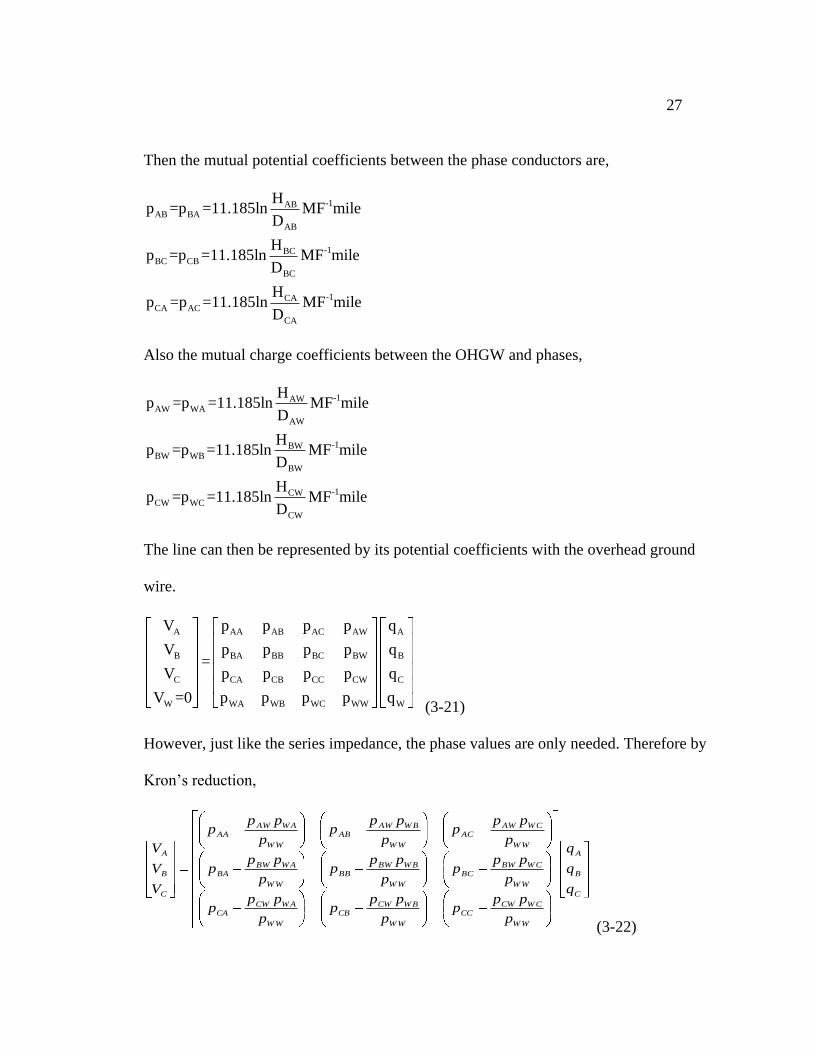
27

Then the mutual potential coefficients between the phase conductors are,

-1ABAB BA

AB

-1BCBC CB

BC

-1CACA AC

CA

Hp =p =11.185ln MF mile

D


D


D

Also the mutual charge coefficients between the OHGW and phases,

-1AWAW WA

AW

-1BWBW WB

BW

-1CWCW WC

CW


D


D


D

The line can then be represented by its potential coefficients with the overhead ground

wire.

A AA AB AC AW A

B BA BB BC BW B

C CA CB CC CW C

W WA WB WC WW W

V p p p p q

V p p p p q=

V p p p p q

V =0 p p p p q (3-21)

However, just like the series impedance, the phase values are only needed. Therefore by

Kron’s reduction,

C

B

A

W W

W CCWCC

W W

W BCWCB

W W

W ACWCA

W W

W CBWBC

W W

W BBWBB

W W

W ABWBA

W W

W CAWAC

W W

W BAWAB

W W

W AAWAA

C

B

A

q

q

q

p

ppp

p

ppp

p

ppp

p

ppp

p

ppp

p

ppp

p

ppp

p

ppp

p

ppp

V

V

V

(3-22)

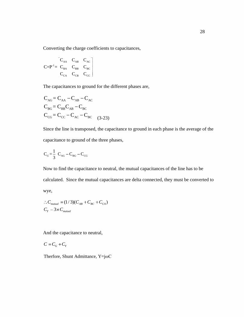
28

Converting the charge coefficients to capacitances,

AA AB AC

-1

BA BB BC

CA CB CC

C C C

C=P = C C C

C C C

The capacitances to ground for the different phases are,

AG AA AB AC

BG BB AB BC

CG CC AC BC

C = C C C

C = C C C

C = C C C (3-23)

Since the line is transposed, the capacitance to ground in each phase is the average of the

capacitance to ground of the three phases,

AG BG CG

1C = C C C

3G

Now to find the capacitance to neutral, the mutual capacitances of the line has to be

calculated. Since the mutual capacitances are delta connected, they must be converted to

wye,

(1/ 3)( )

3

mutual AB BC CA

Y mutual

C C C C

C C

And the capacitance to neutral,

G YC C C

Therfore, Shunt Admittance, Y=jωC

29

3.3 LONG LINE MODEL

Since the lines are so long (150 mi or more), it is not an accurate way to calculate for the

voltage and currents assuming the parameters to be lumped. Various points should be

considered anywhere along the line to fully have the most precise values that are being

desired. Figure 3.6 is used to find the equations for the voltage and current equations.

From Kirchoff’s voltage and current law, Voltage and current can be expressed with

relation between sending and receiving as:

V(x+Δx)=V(x) + zΔxI(x)

V(x+Δx) V(x)=zI(x) (1)

Δx

(3-24)

I(x+Δx)=I(x)+yΔxV(x+Δx)

I(x+Δx)-I(x)=yV(x+Δx) (2)

Δx

Taking the limit as x 0of eqn. (1) and (2),

dV(x) V(x) V(x) 0= = L'hopital=zI(x) (3)

dx Δx 0

dI(x) I(x) I(x) 0= = L'hopital=yV(x) (4)

dx Δx 0

2

2

d V(x) dI(x) =z (5)

dx dx

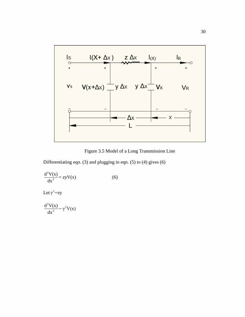
30

Figure 3.5 Model of a Long Transmission Line

Differentiating eqn. (3) and plugging in eqn. (5) to (4) gives (6)

2

2

d V(x)= zyV(x) (6)

dx

Let 2γ =zy

22

2

d V(x)γ V(x)

dx

31

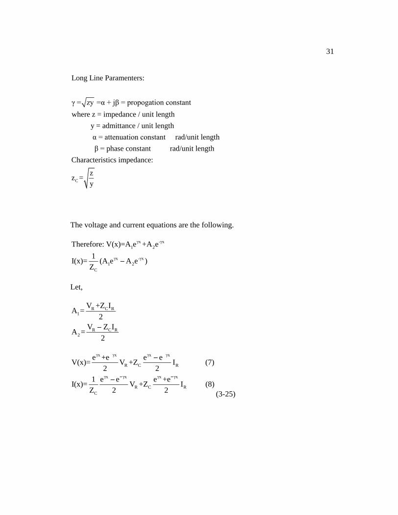
Long Line Paramenters:

γ = zy =α + jβ = propogation constant

where z = impedance / unit length

y = admittance / unit length

α = attenuation constant rad/unit length

β =

C

phase constant rad/unit length

Characteristics impedance:

zz =

y

The voltage and current equations are the following.

γx -γx

1 2

γx -γx

1 2

C

Therefore: V(x)=A e +A e

1I(x)= (A e A e )

Z

Let,

R C R1

R C R2

V +Z IA =

2

V Z IA =

2

γx γx γx γx

R C R

γx γx γx γx

R C R

C

e +e e eV(x)= V +Z I (7)

2 2

1 e e e +eI(x)= V +Z I (8)

Z 2 2(3-25)

32

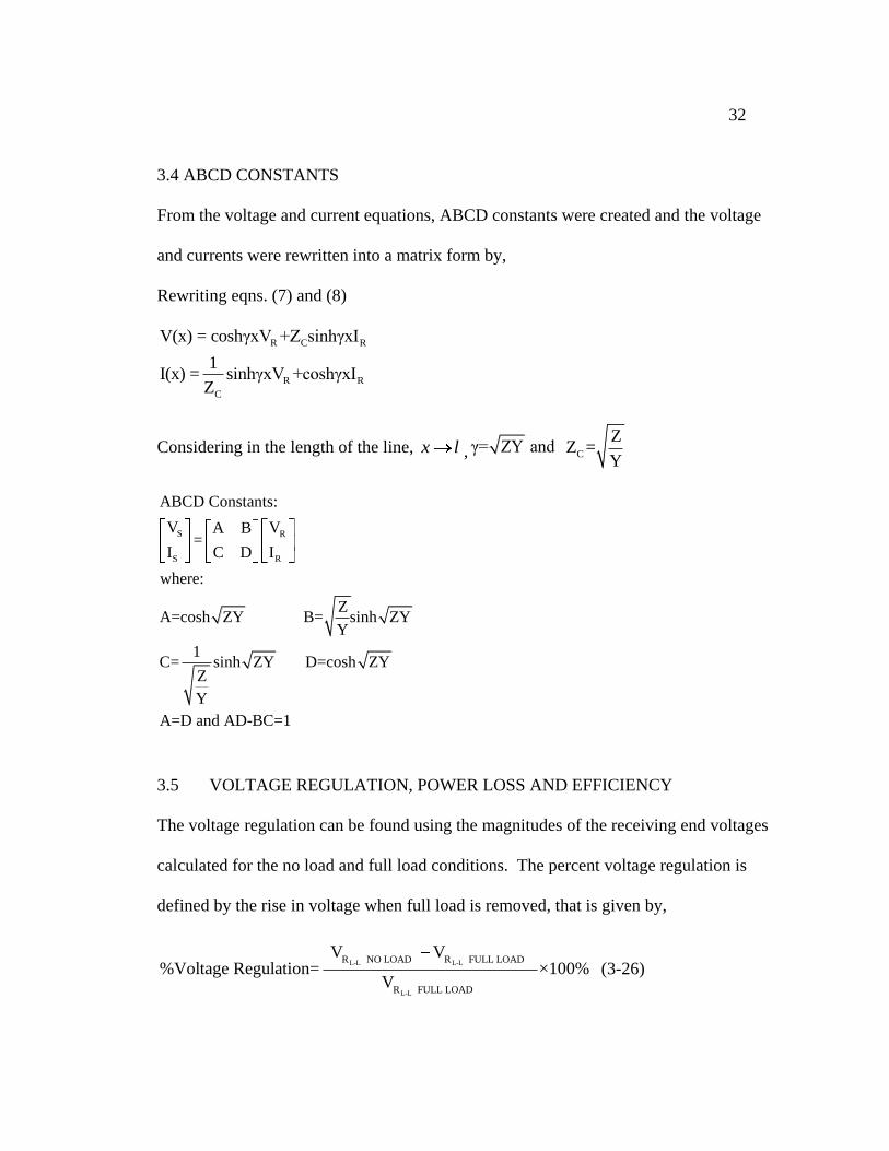
3.4 ABCD CONSTANTS

From the voltage and current equations, ABCD constants were created and the voltage

and currents were rewritten into a matrix form by,

Rewriting eqns. (7) and (8)

R C R

R R

C

V(x) = coshγxV +Z sinhγxI

1I(x) = sinhγxV +coshγxI

Z

Considering in the length of the line, x l , γ= ZY and C

ZZ =

Y

S R

S R

ABCD Constants:

V VA B=

I C D I

where:

ZA=cosh ZY B= sinh ZY

Y

1C= sinh ZY D=cosh ZY

Z

Y

A=D and AD-BC=1

3.5 VOLTAGE REGULATION, POWER LOSS AND EFFICIENCY

The voltage regulation can be found using the magnitudes of the receiving end voltages

calculated for the no load and full load conditions. The percent voltage regulation is

defined by the rise in voltage when full load is removed, that is given by,

L-L L-L

L-L

R NO LOAD R FULL LOAD

R FULL LOAD

V V%Voltage Regulation= ×100%

V (3-26)

33

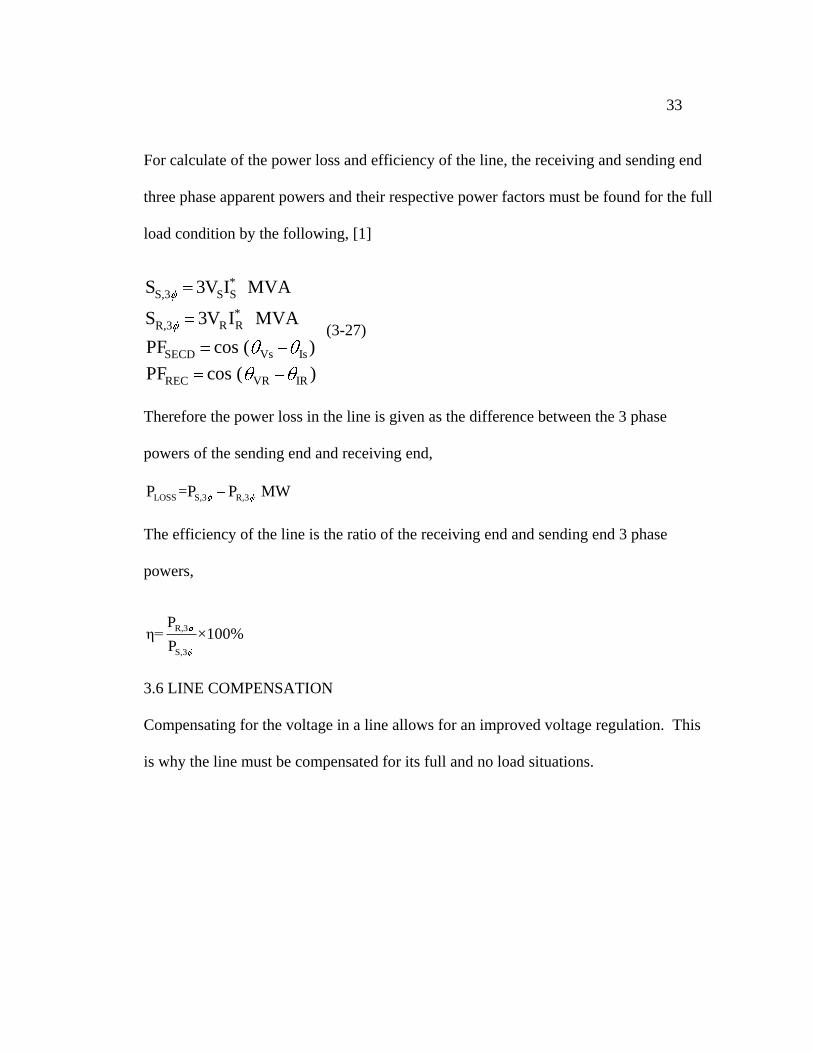
For calculate of the power loss and efficiency of the line, the receiving and sending end

three phase apparent powers and their respective power factors must be found for the full

load condition by the following, [1]

*S,3 S S

*R RR,3

Vs IsSECD

VR IRREC

S 3V I MVA

S 3V I MVA

PF cos ( )

PF cos ( )

(3-27)

Therefore the power loss in the line is given as the difference between the 3 phase

powers of the sending end and receiving end,

LOSS S,3 R,3P =P P MW

The efficiency of the line is the ratio of the receiving end and sending end 3 phase

powers,

R,3

S,3

Pη= ×100%

P

3.6 LINE COMPENSATION

Compensating for the voltage in a line allows for an improved voltage regulation. This

is why the line must be compensated for its full and no load situations.

34

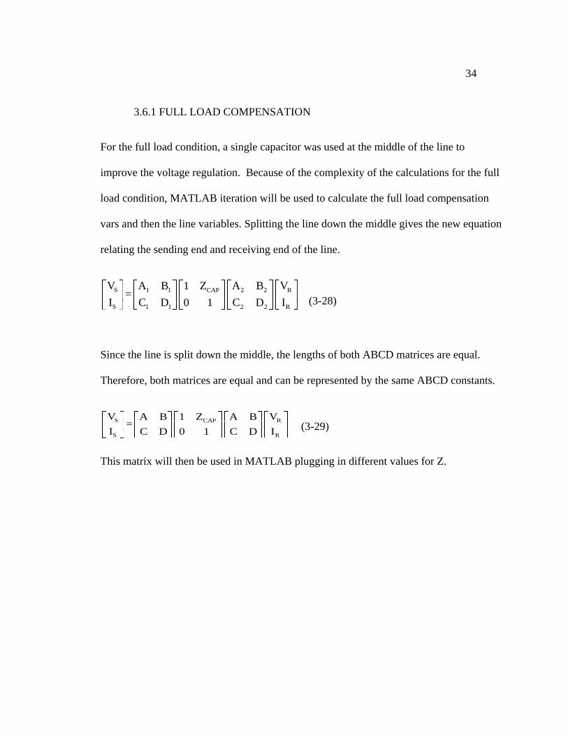
3.6.1 FULL LOAD COMPENSATION

For the full load condition, a single capacitor was used at the middle of the line to

improve the voltage regulation. Because of the complexity of the calculations for the full

load condition, MATLAB iteration will be used to calculate the full load compensation

vars and then the line variables. Splitting the line down the middle gives the new equation

relating the sending end and receiving end of the line.

S 1 1 2 2 RCAP

S 1 1 2 2 R

V A B A B V1 Z=

I C D C D I0 1 (3-28)

Since the line is split down the middle, the lengths of both ABCD matrices are equal.

Therefore, both matrices are equal and can be represented by the same ABCD constants.

(3-29)

This matrix will then be used in MATLAB plugging in different values for Z.

S RCAP

S R

V VA B 1 Z A B=

I IC D 0 1 C D

35

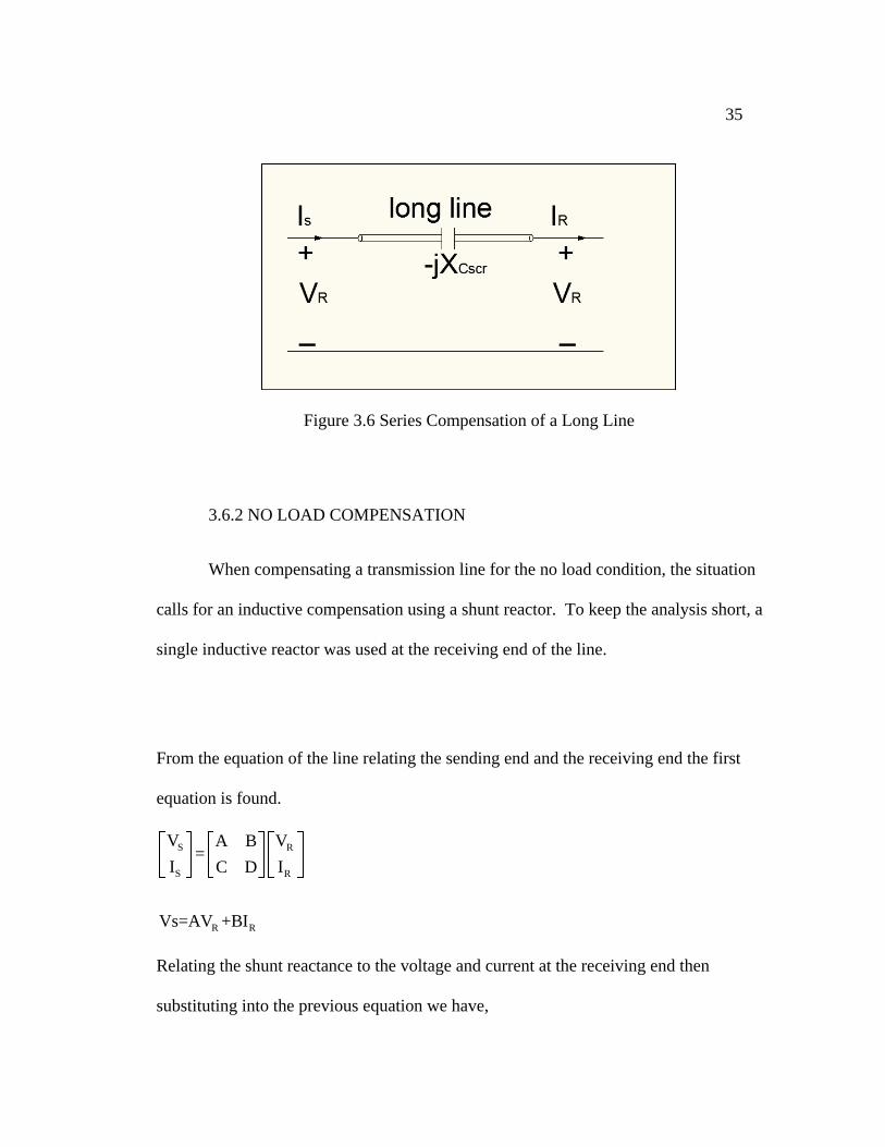
Figure 3.6 Series Compensation of a Long Line

3.6.2 NO LOAD COMPENSATION

When compensating a transmission line for the no load condition, the situation

calls for an inductive compensation using a shunt reactor. To keep the analysis short, a

single inductive reactor was used at the receiving end of the line.

From the equation of the line relating the sending end and the receiving end the first

equation is found.

S R

S R

R R

V VA B=

I IC D

Vs=AV +BI

Relating the shunt reactance to the voltage and current at the receiving end then

substituting into the previous equation we have,

36

sh

sh

RR

L

RR

L

VI =

jX

VVs=AV +B

jX

(3-30)

Solving for the reactance,

sh

R RL

S R S R

S

BV BVjX = =

V -AV V δ-AV

where δ is the angle of V

(3-31)

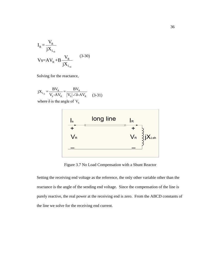
Figure 3.7 No Load Compensation with a Shunt Reactor

Setting the receiving end voltage as the reference, the only other variable other than the

reactance is the angle of the sending end voltage. Since the compensation of the line is

purely reactive, the real power at the receiving end is zero. From the ABCD constants of

the line we solve for the receiving end current.

37

S R R

S RR

S A R

R

B

S R

R B A B

V =AV +BI

V AVI =

B

changing into its phasor notation,

V δ A θ V 0I =

B θ

V A VI = δ θ θ θ

B B

(3-32)

From the equation of three phase power the current is substituted,

*

R,3 R R

*

S R°

R,3 R B A B

2

R S R

R,3 B B A

S =3V I

V A VS =3 V 0 δ θ θ θ

B B

3 V V 3 A VS = θ δ θ θ

B B

(3-33)

Now only the real power equation is needed to find the angle of the sending end voltage,

38

R,3

2

R S R

R,3 B B A

2

R S R

B B A

Therfore, P =0

3 V V 3 A VP = cos θ δ cos θ θ =0

B B

3 V V 3 A Vcos θ δ = cos θ θ

B B

(3-34)

Solving for the sending end voltage angle,

-1

B B A

Aδ=θ cos cos θ θ

R

S

V

V (3-35)

Now the two equations can be put together and the shunt inductive reactance can be

found by,

sh

RL

-1

S B B A R

BVjX = Ohms

AV θ cos cos θ θ AVR

S

V

V

(3-36)

Also the shunt reactor to be installed must have a Mvar rating that corresponds to the

reactance found where,

sh

2

L

3 VQ = var

3 X

R

39

Chapter 4

APPLICATION OF THE MATHEMATICAL MODEL

4.1 INTRODUCTION

A load of 200MVA at a lagging power factor of 0.95 will be located 170 miles out from

the point of origin. A 7 No. 8 Alumoweld Overhead Ground Wire for protection and an

earth resistivity of 100 Ohm meters will be used. Also, a minimum line size of 1/0

ACSR will be understood for structural limitations. Assuming the pre-design

specifications call for a 345kV transposed line, a comparison of the different lines will be

made for their no and full load scenarios. These comparisons will be done based on their

uncompensated & compensated values. In the case of the uncompensated line values, the

voltage rise for the no load situation and the voltage drop for the full load situation will

be calculated by hand.

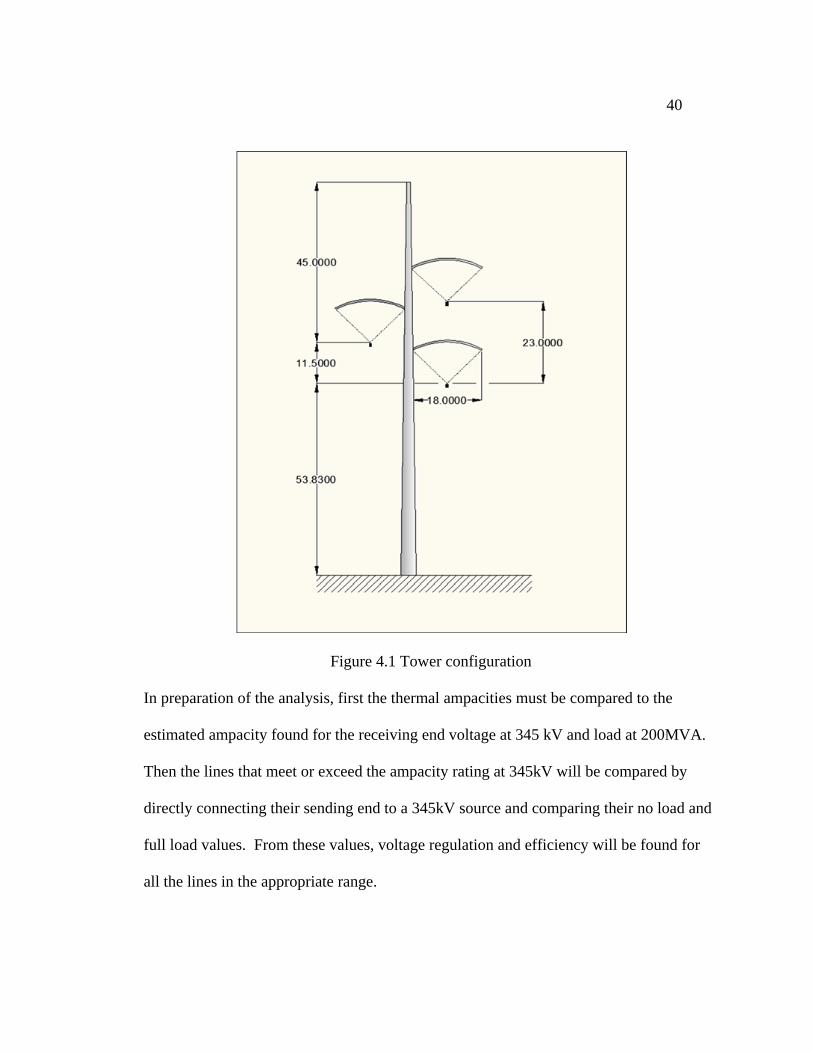
For the analysis, many assumptions were made. For one, the tower configuration of the

line was randomly chosen based on a standard 345kV tower design. The height of the

lowest conductor was set to 53.83 feet at the towers. Two, the load was assumed to be a

worst case scenario and future growth was already considered. Three, all the mechanical

and structural considerations were not considered in the calculations. Other than the

minimum line size of 1/0 ACSR all else will be neglected. And four, different line types

will be compared from among the different sizes of ACSR conductors. Other types of

conductors will be omitted from our analysis.

40

Figure 4.1 Tower configuration

In preparation of the analysis, first the thermal ampacities must be compared to the

estimated ampacity found for the receiving end voltage at 345 kV and load at 200MVA.

Then the lines that meet or exceed the ampacity rating at 345kV will be compared by

directly connecting their sending end to a 345kV source and comparing their no load and

full load values. From these values, voltage regulation and efficiency will be found for

all the lines in the appropriate range.

41

For the application, only the two extremes of the spectrum will be analyzed and

compensated. There are many ways of compensating a line, but the very basic

methodology will be used. The receiving end voltage will be compensated to a 100% for

both situations which sets the magnitudes of the receiving and sending end voltage equal

to each other. For the open circuit situation, a single shunt reactor will be used at the

receiving end of the line to compensate for the voltage. For the full load situation, a

series capacitor compensation will be used midway of the transmission line. A

MATLAB program will be used to verify the hand calculations that will be done and it

will also, instantly calculate the same parameters obtained from the hand calculations but

for all other lines in the range.

4.2 THERMAL AMPACITY RATING

The first step in our search is to figure out which lines meet the thermal ampacity rating.

From the equation for three phase apparent power with the receiving end voltage at

345kV,

(2.1)

From the ACSR table in appendix B, our current of 334.696 Amps could be handled by a

#1 AWG. But since we are limited to 1/0, we will start our analysis from there.

R(3 )

R

R(L-L)

S 200MVAI = = =334.69 Amps

3V 3×345kV

42

4.3 LINE CHARACTERISTICS AND ABCD CONSTANTS

The next step in our analysis is to model the line. Figure 4.1 shows the tower

configuration of our line where the distance from the ground to the lowest conductor is at

53.83 feet. In considering the effects of ground on the line impedance the earth condition

is of “average damp earth” with a resistivity of 100 Ohm meters.

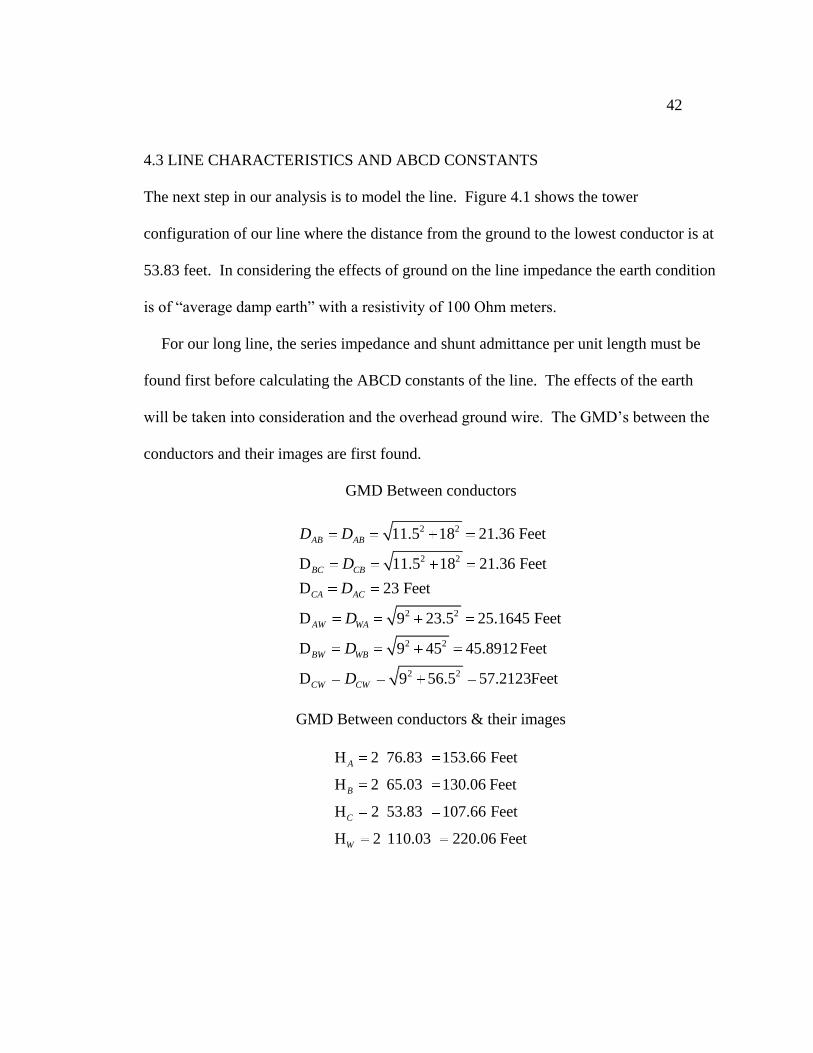
For our long line, the series impedance and shunt admittance per unit length must be

found first before calculating the ABCD constants of the line. The effects of the earth

will be taken into consideration and the overhead ground wire. The GMD’s between the

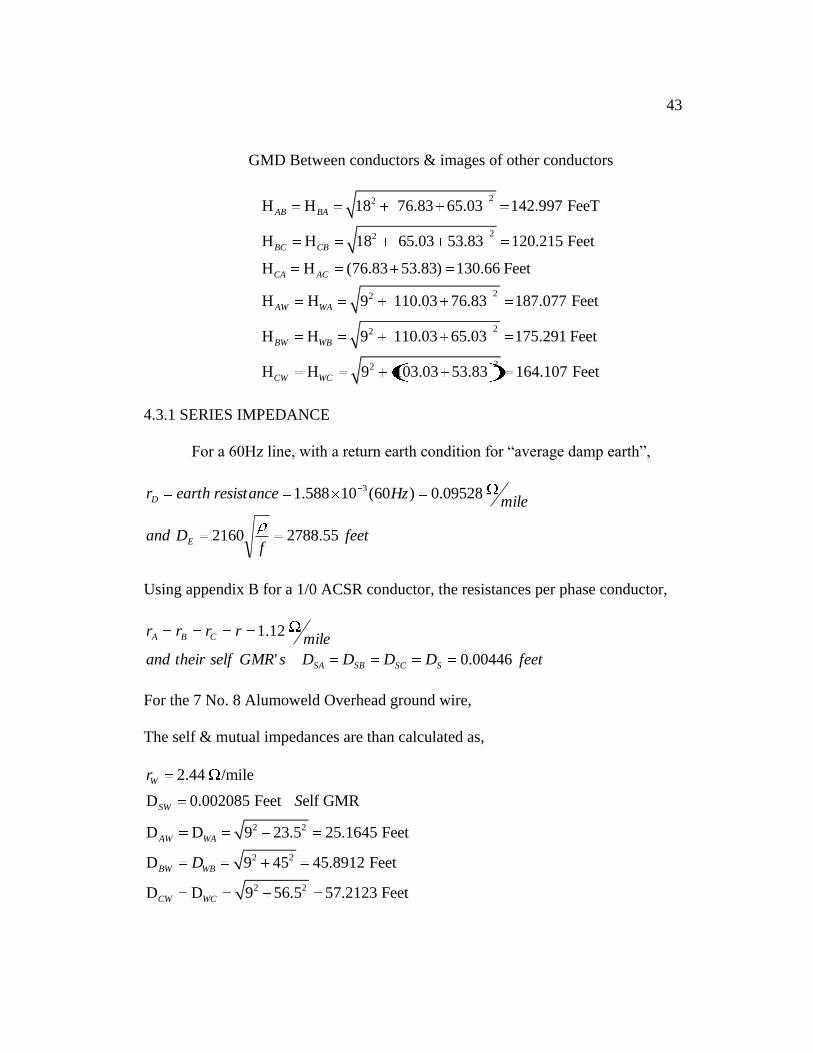
conductors and their images are first found.

GMD Between conductors

2 2

2 2

2 2

2 2

2 2

11.5 18 21.36 Feet

D 11.5 18 21.36 Feet

D 23 Feet

D 9 23.5 25.1645 Feet

D 9 45 45.8912Feet

D 9 56.5 57.2123Feet

AB AB

BC CB

CA AC

AW WA

BW WB

CW CW

D D

D

D

D

D

D

GMD Between conductors & their images

H 2 76.83 153.66 Feet

H 2 65.03 130.06 Feet

H 2 53.83 107.66 Feet

H 2 110.03 220.06 Feet

A

B

C

W

43

GMD Between conductors & images of other conductors

22

22

22

22

2

H H 18 76.83 65.03 142.997 FeeT

H H 18 65.03 53.83 120.215 Feet

H H (76.83 53.83) 130.66 Feet

H H 9 110.03 76.83 187.077 Feet

H H 9 110.03 65.03 175.291 Feet

H H 9 103.03 53

AB BA

BC CB

CA AC

AW WA

BW WB

CW WC

2.83 164.107 Feet

4.3.1 SERIES IMPEDANCE

For a 60Hz line, with a return earth condition for “average damp earth”,

feetf

Dand

mileHzanceresistearthr

E

D

55.27882160

09528.0)60(10588.1 3

Using appendix B for a 1/0 ACSR conductor, the resistances per phase conductor,

feetDDDDsGMRselftheirand

milerrrr

SSCSBSA

CBA

00446.0'

12.1

For the 7 No. 8 Alumoweld Overhead ground wire,

The self & mutual impedances are than calculated as,

2 2

2 2

2 2

2.44 /mile

D 0.002085 Feet elf GMR

D D 9 23.5 25.1645 Feet

D 9 45 45.8912 Feet

D D 9 56.5 57.2123 Feet

W

SW

AW WA

BW WB

CW WC

r

S

D

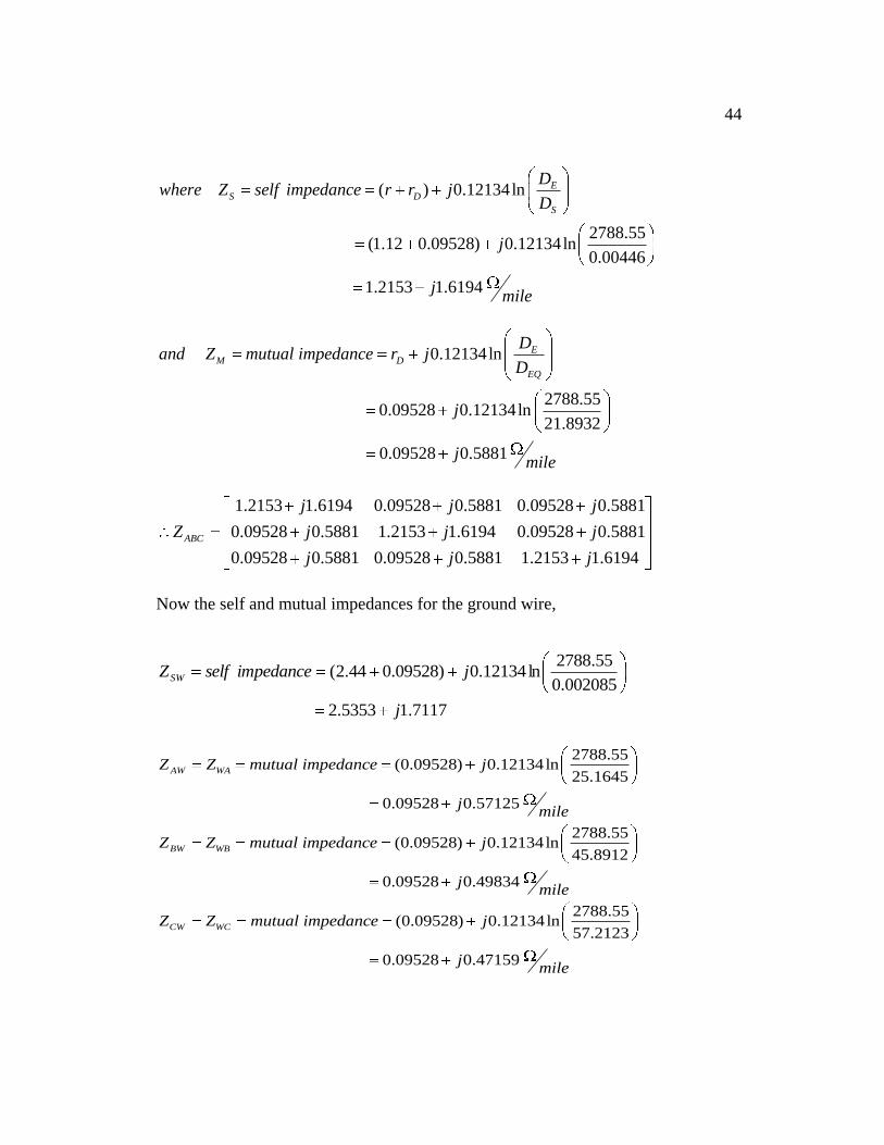
44

( ) 0.12134ln

2788.55(1.12 0.09528) 0.12134ln

0.00446

1.2153 1.6194

ES D

S

Dwhere Z self impedance r r j

D

j

jmile

0.12134ln

2788.550.09528 0.12134ln

21.8932

0.09528 0.5881

EM D

EQ

Dand Z mutual impedance r j

D

j

jmile

1.2153 1.6194 0.09528 0.5881 0.09528 0.5881

0.09528 0.5881 1.2153 1.6194 0.09528 0.5881

0.09528 0.5881 0.09528 0.5881 1.2153 1.6194

ABC

j j j

Z j j j

j j j

Now the self and mutual impedances for the ground wire,

7117.15353.2

002085.0

55.2788ln12134.0)09528.044.2(

j

jimpedanceselfZSW

2788.55(0.09528) 0.12134ln

25.1645

0.09528 0.57125

2788.55(0.09528) 0.12134ln

45.8912

0.09528 0.49834

(0.0

AW WA

BW WB

CW WC

Z Z mutual impedance j

jmile

Z Z mutual impedance j

jmile

Z Z mutual impedance2788.55

9528) 0.12134ln57.2123

0.09528 0.47159

j

jmile

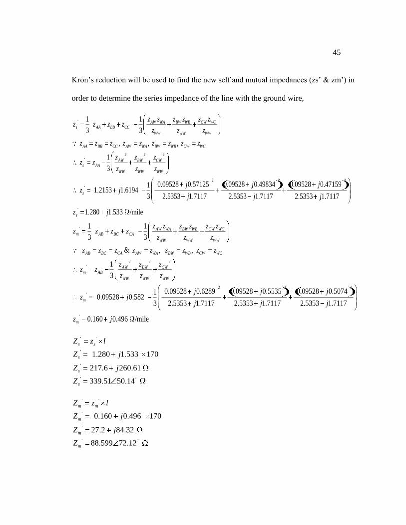
45

Kron’s reduction will be used to find the new self and mutual impedances (zs’ & zm’) in

order to determine the series impedance of the line with the ground wire,

'

2 2 2'

2

'

1 1

3 3

, , ,

1

3

0.09528 0.57125 0.095281 1.2153 1.6194

3 2.5353 1.7117

AW WA BW WB CW WCs AA BB CC

WW WW WW

AA BB CC AW WA BW WB CW WC

AW BW CWs AA

WW WW WW

s

z z z z z zz z z z

z z z

z z z z z z z z z

z z zz z

z z z

j jz j

j

2 2

'

0.49834 0.09528 0.47159

2.5353 1.7117 2.5353 1.7117

1.280 1.533 /miles

j

j j

z j

'

2 2 2'

2

'

1 1

3 3

& , ,

1

3

0.09528 0.6289 0.09528 01 0.09528 0.582

3 2.5353 1.7117

AW WA BW WB CW WCm AB BC CA

WW WW WW

AB BC CA AW WA BW WB CW WC

AW BW CWm AB

WW WW WW

m

z z z z z zz z z z

z z z

z z z z z z z z z

z z zz z

z z z

j jz j

j

2 2

'

.5535 0.09528 0.5074

2.5353 1.7117 2.5353 1.7117

0.160 0.496 /milem

j

j j

z j

' '

'

'

'

1.280 1.533 170

217.6 260.61

339.51 50.14

s s

s

s

s

Z z l

Z j

Z j

Z

' '

'

'

'

0.160 0.496 170

27.2 84.32

88.599 72.12

m m

m

m

m

Z z l

Z j

Z j

Z

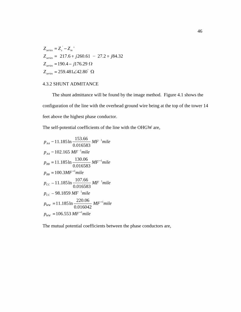
46

' '

217.6 260.61 27.2 84.32

190.4 176.29

259.481 42.80

series s m

series

series

series

Z Z Z

Z j j

Z j

Z

4.3.2 SHUNT ADMITANCE

The shunt admittance will be found by the image method. Figure 4.1 shows the

configuration of the line with the overhead ground wire being at the top of the tower 14

feet above the highest phase conductor.

The self-potential coefficients of the line with the OHGW are,

1

1

1

1

1

1

1

153.6611.185ln

0.016583

102.165

130.0611.185ln

0.016583

100.3

107.6611.185ln

0.016583

98.1859

220.0611.185ln

0.016042

106.

AA

AA

BB

BB

CC

CC

WW

WW

p MF mile

p MF mile

p MF mile

p MF mile

p MF mile

p MF mile

p MF mile

p 1553 MF mile

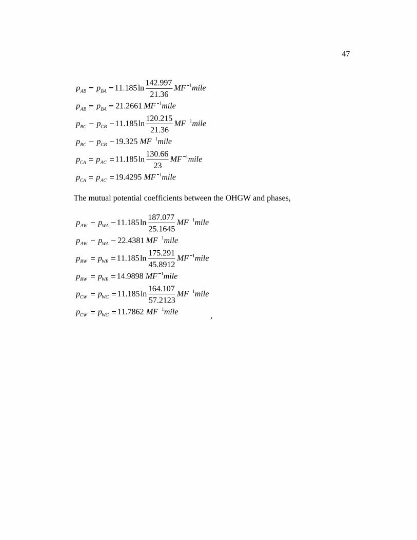
The mutual potential coefficients between the phase conductors are,

47

1

1

1

1

1

1

142.99711.185ln

21.36

21.2661

120.21511.185ln

21.36

19.325

130.6611.185ln

23

19.4295

AB BA

AB BA

BC CB

BC CB

CA AC

CA AC

p p MF mile

p p MF mile

p p MF mile

p p MF mile

p p MF mile

p p MF mile

The mutual potential coefficients between the OHGW and phases,

1

1

1

1

1

1

187.07711.185ln

25.1645

22.4381

175.29111.185ln

45.8912

14.9898

164.10711.185ln

57.2123

11.7862

AW WA

AW WA

BW WB

BW WB

CW WC

CW WC

p p MF mile

p p MF mile

p p MF mile

p p MF mile

p p MF mile

p p MF mile,

48

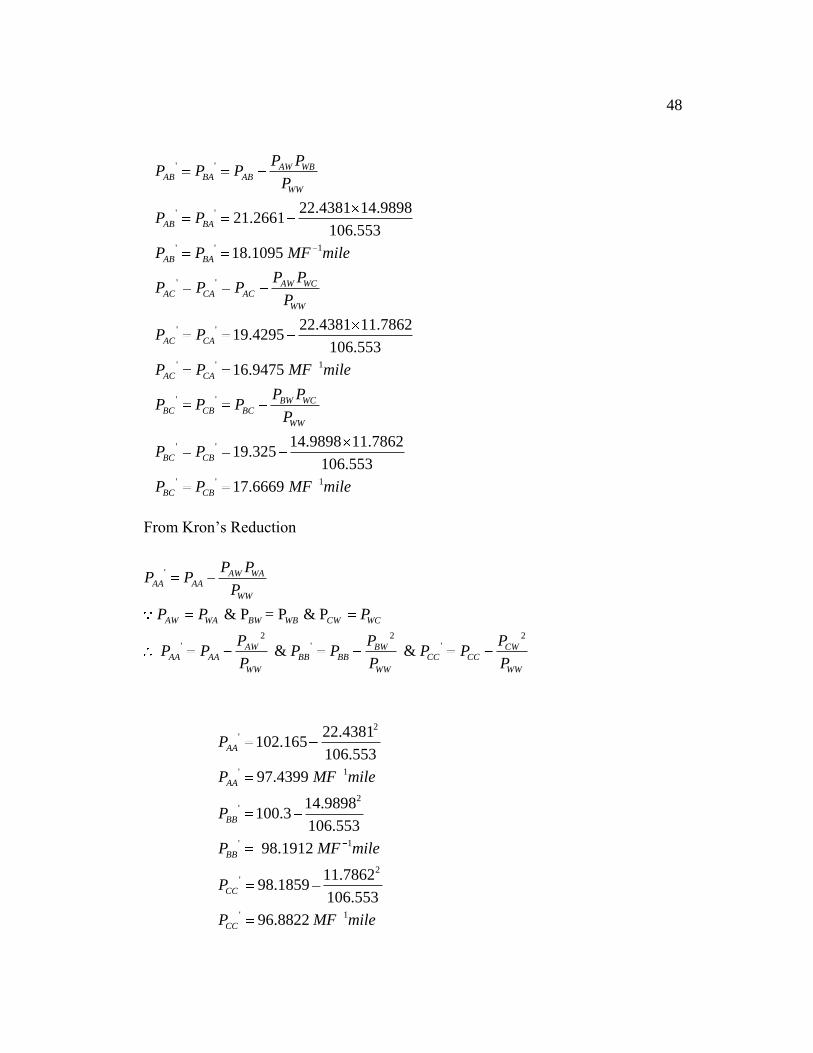
From Kron’s Reduction

' '

' '

' ' 1

' '

' '

' ' 1

' '

22.4381 14.989821.2661

106.553

18.1095

22.4381 11.786219.4295

106.553

16.9475

AW WBAB BA AB

WW

AB BA

AB BA

AW WCAC CA AC

WW

AC CA

AC CA

BW WCBC CB BC

W

P PP P P

P

P P

P P MF mile

P PP P P

P

P P

P P MF mile

P PP P P

P

' '

' ' 1

14.9898 11.786219.325

106.553

17.6669

W

BC CB

BC CB

P P

P P MF mile

'

2 2 2' ' '

& P = P & P

& &

AW WAAA AA

WW

AW WA BW WB CW WC

AW BW CWAA AA BB BB CC CC

WW WW WW

P PP P

P

P P P

P P PP P P P P P

P P P

2'

' 1

2'

' 1

2'

' 1

22.4381102.165

106.553

97.4399

14.9898100.3

106.553

98.1912

11.786298.1859

106.553

96.8822

AA

AA

BB

BB

CC

CC

P

P MF mile

P

P MF mile

P

P MF mile

49

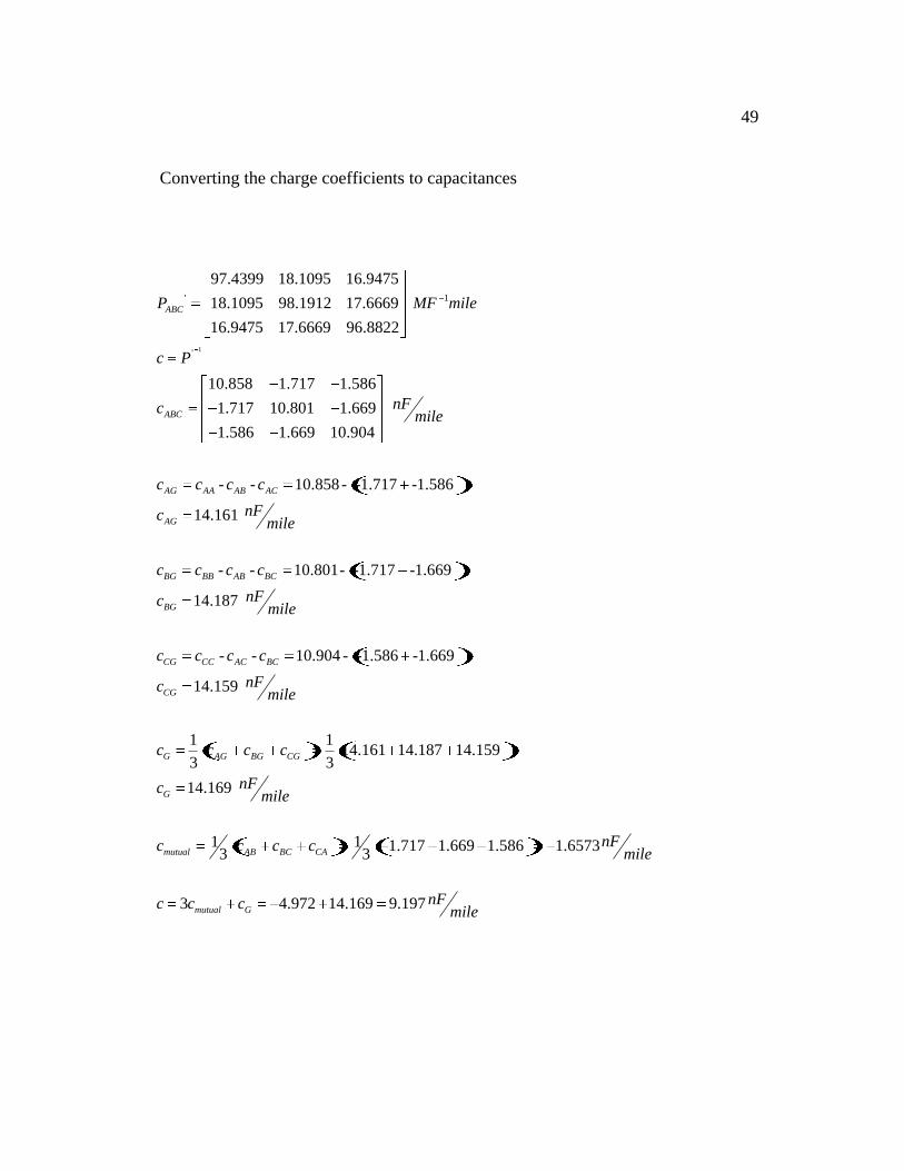
Converting the charge coefficients to capacitances

1

' 1

'

97.4399 18.1095 16.9475

18.1095 98.1912 17.6669

16.9475 17.6669 96.8822

10.858 1.717 1.586

1.717 10.801 1.669

1.586 1.669 10.904

- - 10.858 - -1.717

ABC

ABC

AG AA AB AC

P MF mile

c P

nFcmile

c c c c -1.586

14.161

- - 10.801- -1.717 -1.669

14.187

- - 10.904 - -1.586 -1.669

14.159

1 114.161 14.187 14.159

3 3

14.169

13

AG

BG BB AB BC

BG

CG CC AC BC

CG

G AG BG CG

G

mutual AB

nFcmile

c c c c

nFcmile

c c c c

nFcmile

c c c c

nFcmile

c c 1 1.717 1.669 1.586 1.65733

3 4.972 14.169 9.197

BC CA

mutual G

nFc cmile

nFc c cmile

50

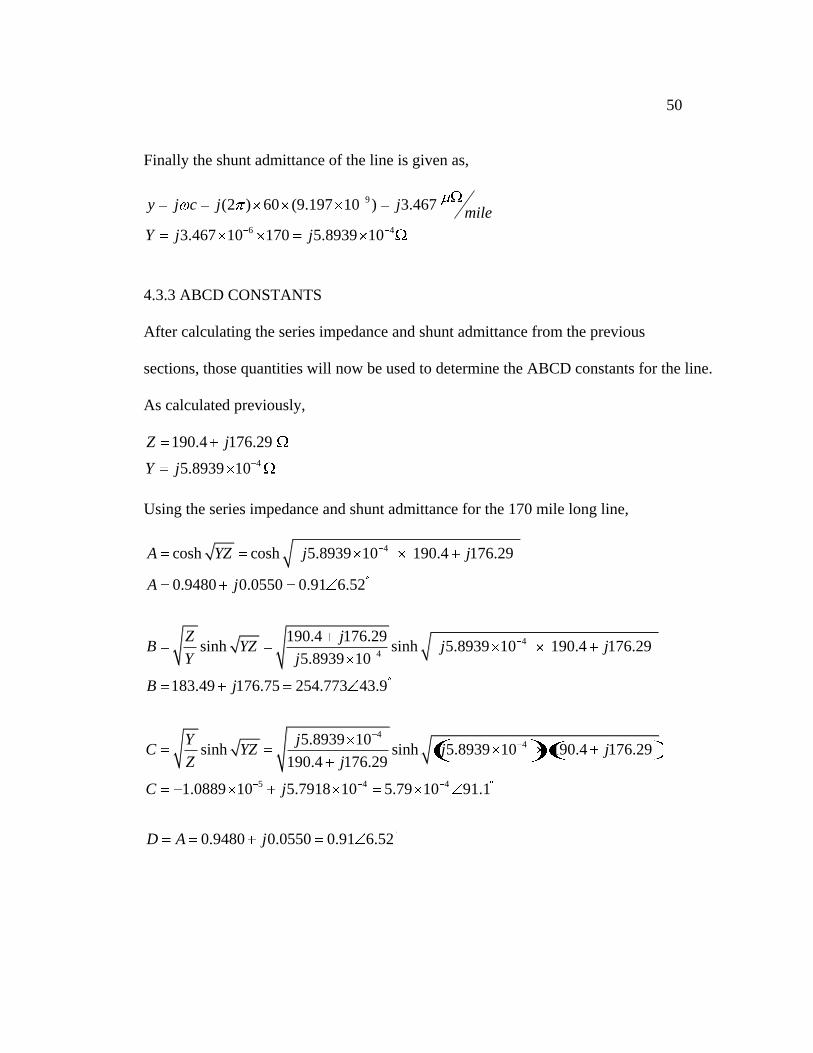
Finally the shunt admittance of the line is given as,

9

6 4

(2 ) 60 (9.197 10 ) 3.467

3.467 10 170 5.8939 10

y j c j jmile

Y j j

4.3.3 ABCD CONSTANTS

After calculating the series impedance and shunt admittance from the previous

sections, those quantities will now be used to determine the ABCD constants for the line.

As calculated previously,

4

190.4 176.29

5.8939 10

Z j

Y j

Using the series impedance and shunt admittance for the 170 mile long line,

4

4

4

4

cosh cosh 5.8939 10 190.4 176.29

0.9480 0.0550 0.91 6.52

190.4 176.29sinh sinh 5.8939 10 190.4 176.29

5.8939 10

183.49 176.75 254.773 43.9

5.8939 10sinh si

190.4 176.29

A YZ j j

A j

Z jB YZ j j

Y j

B j

Y jC YZ

Z j

4

5 4 4

nh 5.8939 10 190.4 176.29

1.0889 10 5.7918 10 5.79 10 91.1

0.9480 0.0550 0.91 6.52

j j

C j

D A j

51

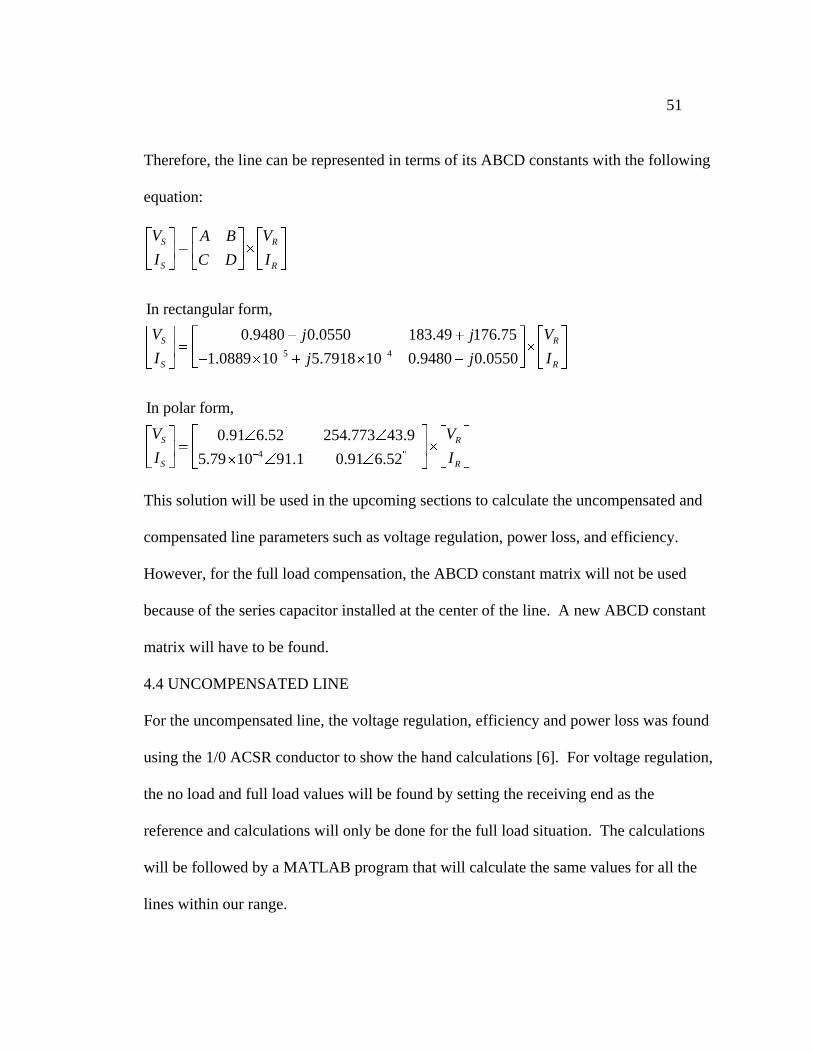
Therefore, the line can be represented in terms of its ABCD constants with the following

equation:

5 4

In rectangular form,

0.9480 0.0550 183.49 176.75

1.0889 10 5.7918 10 0.9480 0.0550

In polar form,

0.91 6.52 254.773 43.9

5.79

S R

S R

S R

S R

S

S

V VA B

I IC D

V Vj j

I Ij j

V

I 410 91.1 0.91 6.52

R

R

V

I

This solution will be used in the upcoming sections to calculate the uncompensated and

compensated line parameters such as voltage regulation, power loss, and efficiency.

However, for the full load compensation, the ABCD constant matrix will not be used

because of the series capacitor installed at the center of the line. A new ABCD constant

matrix will have to be found.

4.4 UNCOMPENSATED LINE

For the uncompensated line, the voltage regulation, efficiency and power loss was found

using the 1/0 ACSR conductor to show the hand calculations [6]. For voltage regulation,

the no load and full load values will be found by setting the receiving end as the

reference and calculations will only be done for the full load situation. The calculations

will be followed by a MATLAB program that will calculate the same values for all the

lines within our range.

52

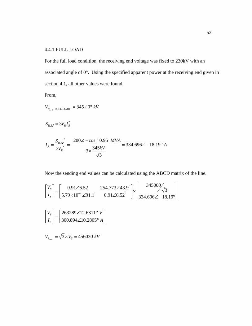
4.4.1 FULL LOAD

For the full load condition, the receiving end voltage was fixed to 230kV with an

associated angle of 0°. Using the specified apparent power at the receiving end given in

section 4.1, all other values were found.

From,

FULL

*

,3

1*

,3

*

345 0

3

200 cos 0.95334.696 18.19

34533

3

L LR LOAD

R R R

R

R

R

V kV

S V I

MVASI A

kVV

Now the sending end values can be calculated using the ABCD matrix of the line.

4

3450000.91 6.52 254.773 43.9

35.79 10 91.1 0.91 6.52 334.696 18.19

263289 12.6311

300.894 10.2805

3 456030 L L

S

S

S

S

S S

V

I

V V

I A

V V kV

53

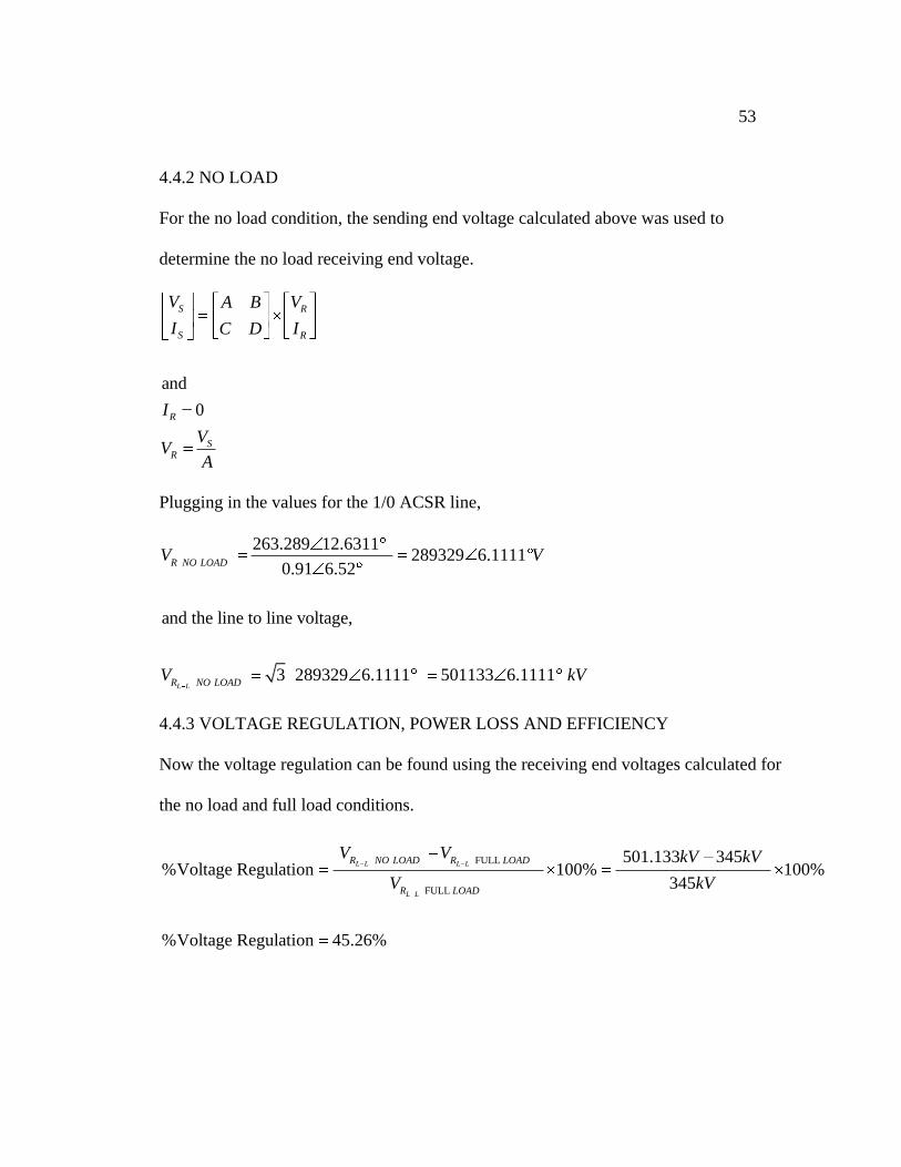
4.4.2 NO LOAD

For the no load condition, the sending end voltage calculated above was used to

determine the no load receiving end voltage.

and

0

S R

S R

R

SR

V VA B

I IC D

I

VV

A

Plugging in the values for the 1/0 ACSR line,

263.289 12.6311 289329 6.1111

0.91 6.52

and the line to line voltage,

3 289329 6.1111 501133 6.1111 L L

R NO LOAD

R NO LOAD

V V

V kV

4.4.3 VOLTAGE REGULATION, POWER LOSS AND EFFICIENCY

Now the voltage regulation can be found using the receiving end voltages calculated for

the no load and full load conditions.

FULL

FULL

501.133 345%Voltage Regulation 100% 100%

345

%Voltage Regulation 45.26%

L L L L

L L

R NO LOAD R LOAD

R LOAD

V V kV kV

V kV

54

To calculate the power loss and efficiency of the line the receiving end three phase

powers are found for the full load condition.

*

,3

,3

3 3 263289 12.6311 300.894 10.2805 237.466 9.748

cos cos 12.6311 10.2805 0.9991

190 62.45

S S

S S S

SEND V I

R

S V I j MVA

PF

S j MVA

Therefore the power loss in the line,

,3 ,3 237.466 190 47.466 LOSS S RP P P MW

And the efficiency of the line is,

,3

,3

190100% 80.01%

237.466

R

S

P

P

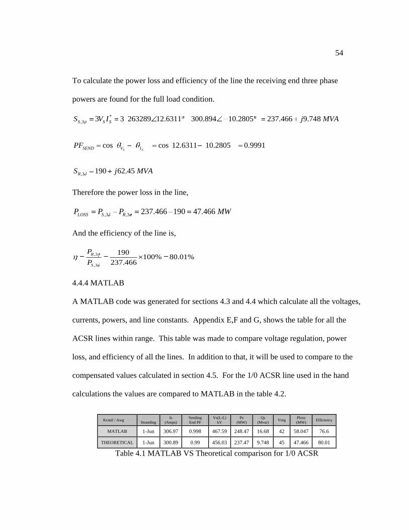
4.4.4 MATLAB

A MATLAB code was generated for sections 4.3 and 4.4 which calculate all the voltages,

currents, powers, and line constants. Appendix E,F and G, shows the table for all the

ACSR lines within range. This table was made to compare voltage regulation, power

loss, and efficiency of all the lines. In addition to that, it will be used to compare to the

compensated values calculated in section 4.5. For the 1/0 ACSR line used in the hand

calculations the values are compared to MATLAB in the table 4.2.

Kcmil / Awg

Stranding

Is

(Amps)

Sending

End PF

Vs(L-L)

kV

Ps

(MW)

Qs

(Mvar) Vreg

Ploss

(MW) Efficiency

MATLAB 1-Jun 306.97 0.998 467.59 248.47 16.68 42 58.047 76.6

THEORETICAL 1-Jun 300.89 0.99 456.03 237.47 9.748 45 47.466 80.01

Table 4.1 MATLAB VS Theoretical comparison for 1/0 ACSR

55

4.5 COMPENSATION

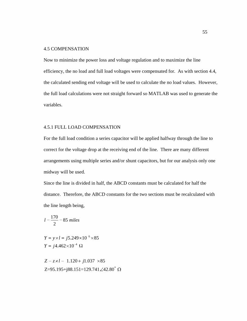
Now to minimize the power loss and voltage regulation and to maximize the line

efficiency, the no load and full load voltages were compensated for. As with section 4.4,

the calculated sending end voltage will be used to calculate the no load values. However,

the full load calculations were not straight forward so MATLAB was used to generate the

variables.

4.5.1 FULL LOAD COMPENSATION

For the full load condition a series capacitor will be applied halfway through the line to

correct for the voltage drop at the receiving end of the line. There are many different

arrangements using multiple series and/or shunt capacitors, but for our analysis only one

midway will be used.

Since the line is divided in half, the ABCD constants must be calculated for half the

distance. Therefore, the ABCD constants for the two sections must be recalculated with

the line length being,

6

4

17085

2

5.249 10 85

4.462 10

1.120 1.037 85

Z=95.195+j88.151=129.741 42.80

l miles

Y y l j

Y j

Z z l j

56

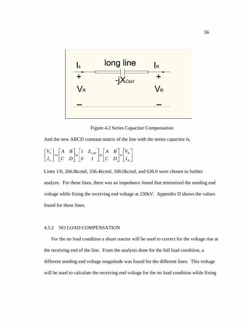
Figure 4.2 Series Capacitor Compensation

And the new ABCD constant matrix of the line with the series capacitor is,

1

0 1

S RCAP

S R

V VA B Z A B

I IC D C D

Lines 1/0, 266.8kcmil, 336.4kcmil, 500.0kcmil, and 636.0 were chosen to further

analyze. For these lines, there was an impedance found that minimized the sending end

voltage while fixing the receiving end voltage at 230kV. Appendix D shows the values

found for these lines.

4.5.2 NO LOAD COMPENSATION

For the no load condition a shunt reactor will be used to correct for the voltage rise at

the receiving end of the line. From the analysis done for the full load condition, a

different sending end voltage magnitude was found for the different lines. This voltage

will be used to calculate the receiving end voltage for the no load condition while fixing

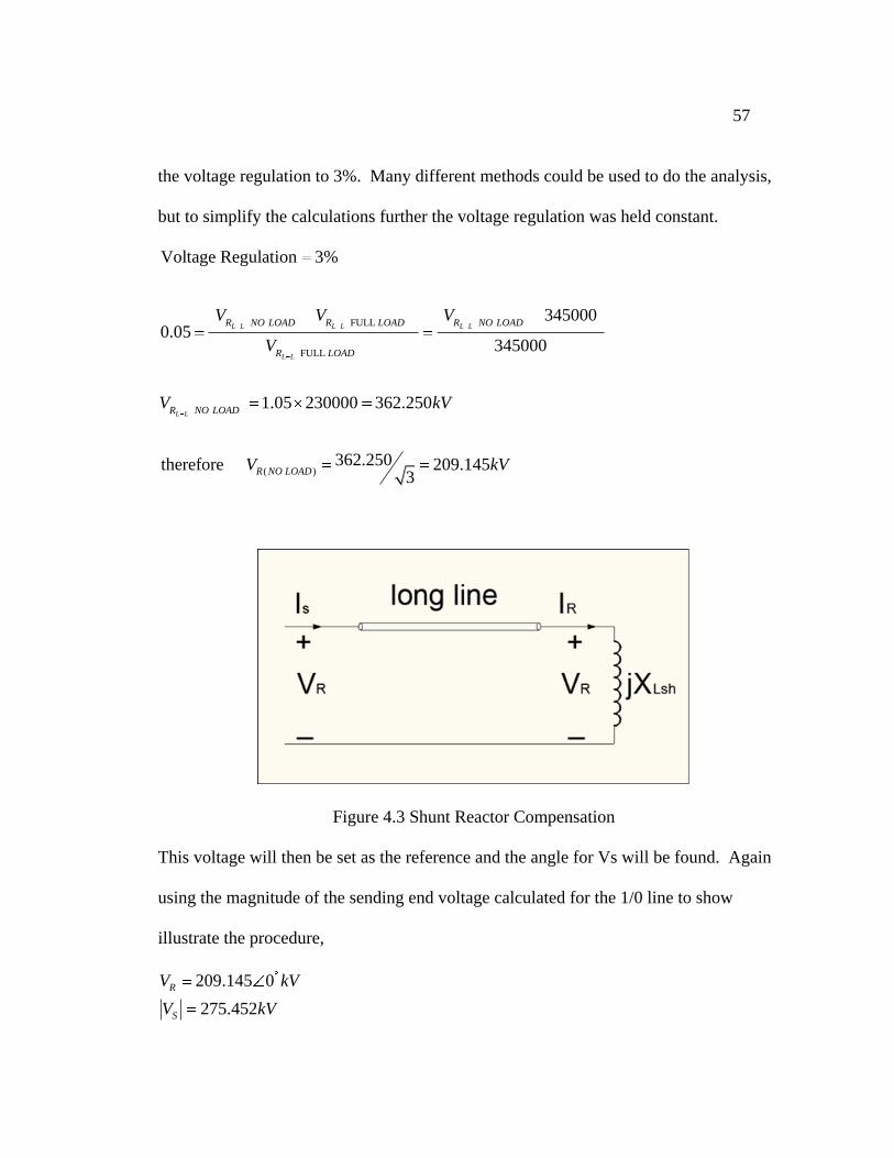
57

the voltage regulation to 3%. Many different methods could be used to do the analysis,

but to simplify the calculations further the voltage regulation was held constant.

FULL

FULL

( )

Voltage Regulation 3%

3450000.05

345000

1.05 230000 362.250

362.250therefore 209.1453

L L L L L L

L L

L L

R NO LOAD R LOAD R NO LOAD

R LOAD

R NO LOAD

R NO LOAD

V V V

V

V kV

V kV

Figure 4.3 Shunt Reactor Compensation

This voltage will then be set as the reference and the angle for Vs will be found. Again

using the magnitude of the sending end voltage calculated for the 1/0 line to show

illustrate the procedure,

209.145 0

275.452

R

S

V kV

V kV

58

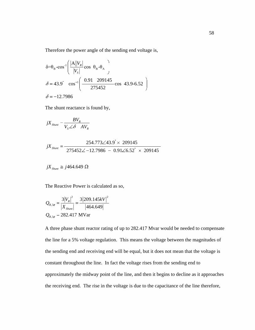
Therefore the power angle of the sending end voltage is,

-1

B B A

1

Aδ=θ -cos cos θ -θ

0.91 20914543.9 cos cos 43.9-6.52

275452

12.7986

R

S

V

V

The shunt reactance is found by,

254.773 43.9 209145

275452 12.7986 0.91 6.52 209145

464.649

RShunt

S R

Shunt

Shunt

BVjX

V AV

jX

jX j

The Reactive Power is calculated as so,

2 2

,3

,3

3 3 209.145

464.649

282.417 MVar

R

R

Shunt

R

V kVQ

X

Q

A three phase shunt reactor rating of up to 282.417 Mvar would be needed to compensate

the line for a 5% voltage regulation. This means the voltage between the magnitudes of

the sending end and receiving end will be equal, but it does not mean that the voltage is

constant throughout the line. In fact the voltage rises from the sending end to

approximately the midway point of the line, and then it begins to decline as it approaches

the receiving end. The rise in the voltage is due to the capacitance of the line therefore,

59

the reactor is used increase the current and the impedance of the line which in turn

decreases the voltage.

60

Chapter 5

SUMMARY

The basis of our analysis was to determine a method of selecting a line based on its

electrical characteristics. These electrical characteristics include but are not limited to

power loss, efficiency, and voltage regulation. However, those three characteristics are

the focus of our analysis. This investigation was made by fixing the full load apparent

power and receiving end voltage to 200MVA at 0.95 lagging power factor and 345kV

respectively. Other parameters that remained constant throughout the analysis were the

tower configuration, line length, and overhead ground wire type. This enabled us keep

the mathematical model as simple as possible without leaving anything out. Once the

lines were modeled, a table was generated for the uncompensated condition to show the

difference in line characteristics as size varies from 1/0 up to 1590kcmil. Then out of the

table, 5 different lines were selected to further investigate its electrical properties.

In solving for the uncompensated condition the full load receiving end voltage was fixed

to 345kV. Then the full load sending end voltage was applied to the no load condition to

calculate the no load receiving end voltage. The analysis showed that for the no load

condition, the voltage drastically increases and for full load condition it decreases. Also,

by varying the line sizes from 1/0 to 1590.0kcmil, as the line size goes up, the full load

sending end voltage goes down while power loss, efficiency, and voltage regulation

improve.

Compensating for the voltage of a transmission line increases its voltage capability. It

also allows for a line to stay within a specified range which is determined by the tower

61

configuration, insulator other hardware ratings. In the compensation section in our

analysis, five different lines were selected to further analyze. These lines were the 1/0,

266.8kcmil 6/7 strand, 336.4kcmil 26/7 strand, 500.0kcmil 30/7 strand, and 636.0kcmil

26/7 strand ACSR conductors. A comparison was first done between the uncompensated

and compensated values found for the different lines. Then a comparison was done

between the 5 lines for the compensated condition.

Now that a basis has been established, the electrical characteristics can then be used to

perform an economic analysis to determine which line to choose. Power loss, power

supplied, and Mvar corrected would be converted to its dollar value and compared

between the different wires and the most economical line will be chosen.

62

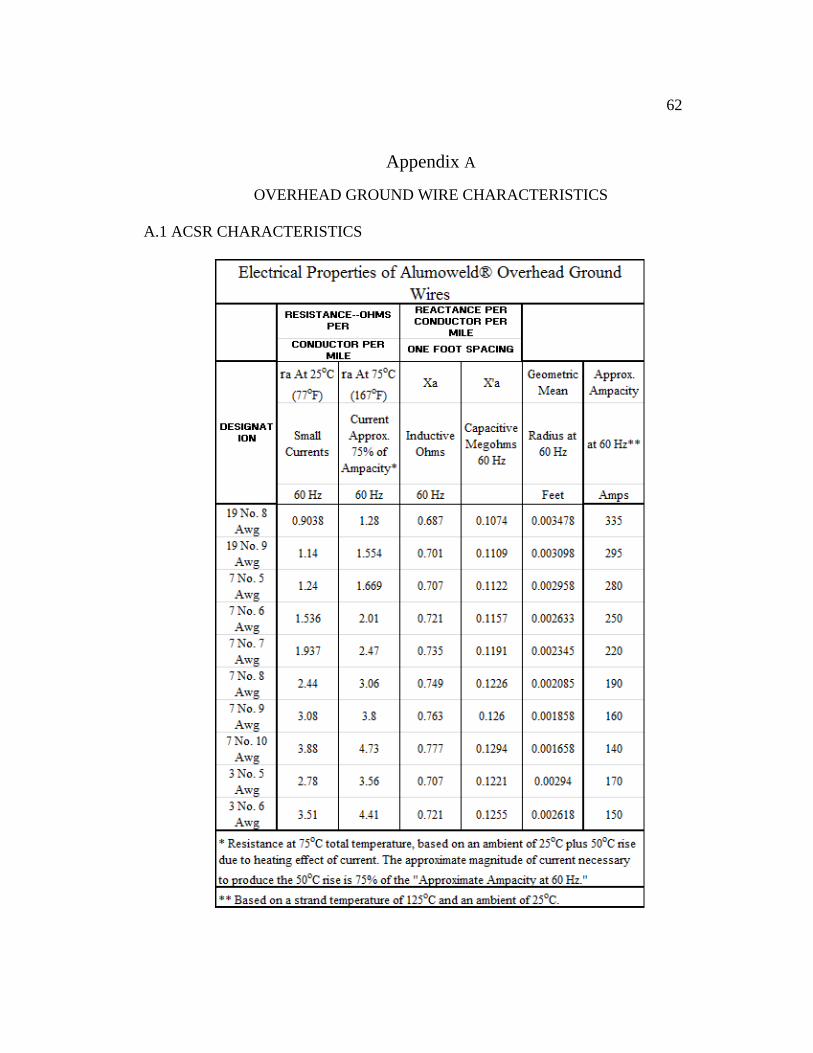
Appendix A OVERHEAD GROUND WIRE CHARACTERISTICS

A.1 ACSR CHARACTERISTICS

63

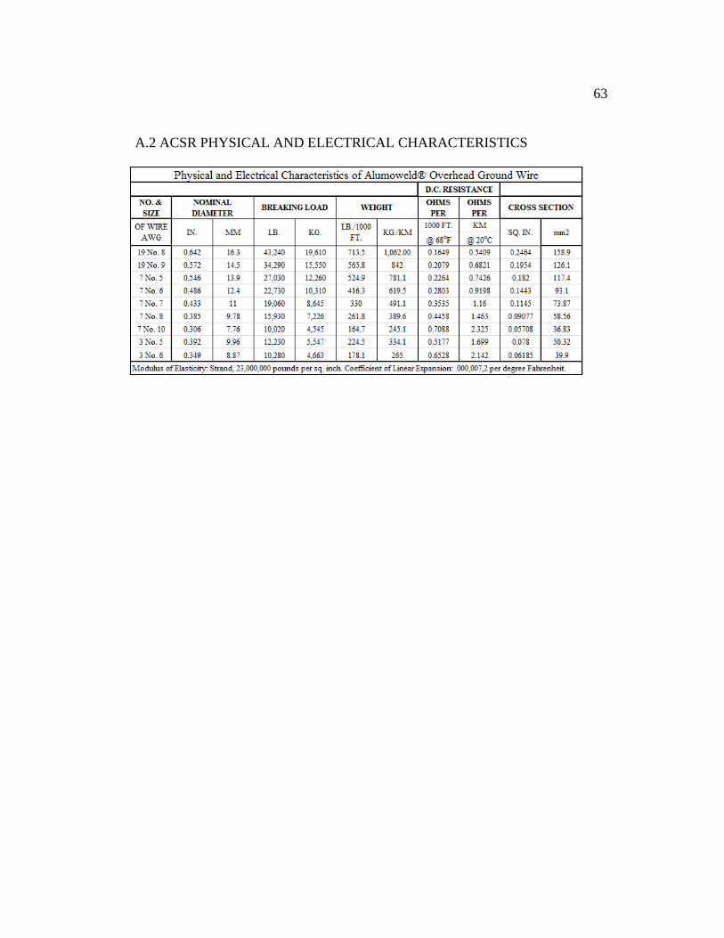
A.2 ACSR PHYSICAL AND ELECTRICAL CHARACTERISTICS

64

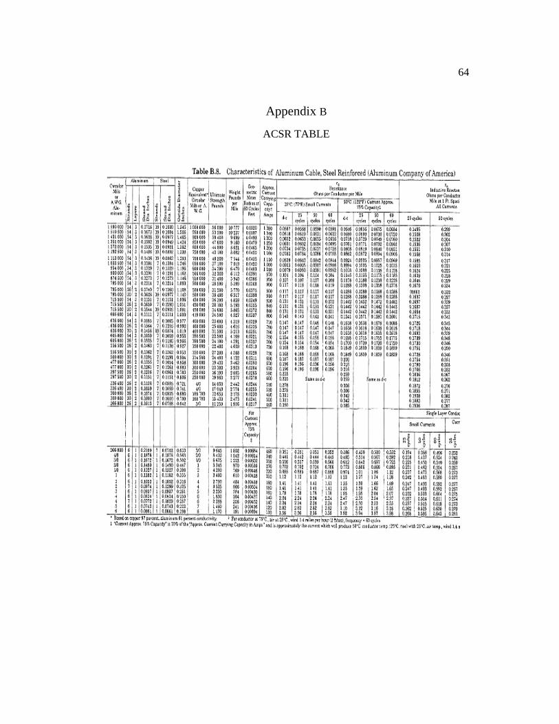
Appendix B

ACSR TABLE

65

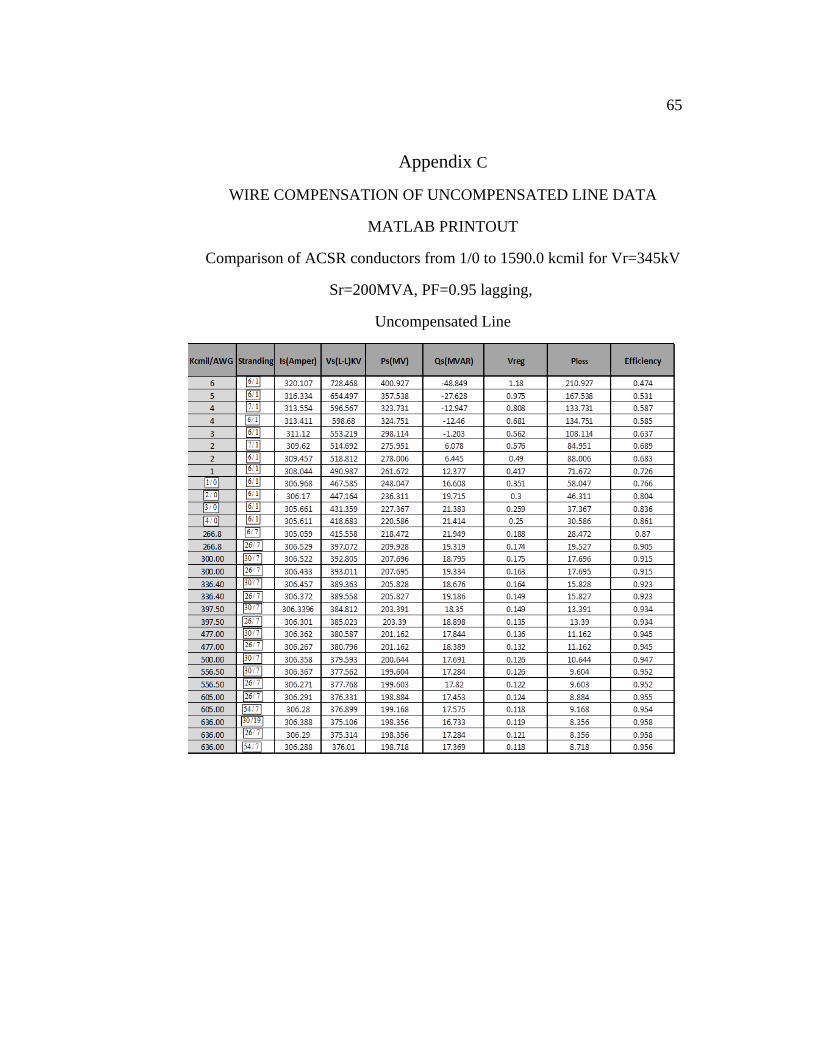
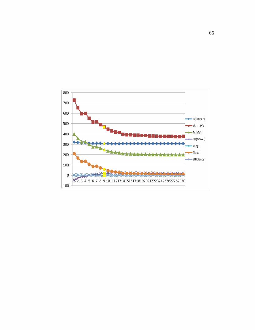
Appendix C

WIRE COMPENSATION OF UNCOMPENSATED LINE DATA

MATLAB PRINTOUT

Comparison of ACSR conductors from 1/0 to 1590.0 kcmil for Vr=345kV

Sr=200MVA, PF=0.95 lagging,

Uncompensated Line

67

Appendix D

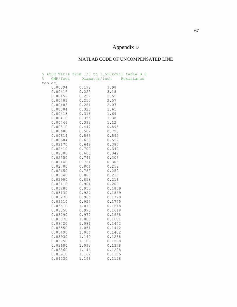
MATLAB CODE OF UNCOMPENSATED LINE

% ACSR Table from 1/0 to 1,590kcmil table B.8 % GMR/feet Diameter/inch Resistance table=[ 0.00394 0.198 3.98 0.00416 0.223 3.18 0.00452 0.257 2.55 0.00401 0.250 2.57 0.00403 0.281 2.07 0.00504 0.325 1.65 0.00418 0.316 1.69 0.00418 0.355 1.38 0.00446 0.398 1.12 0.00510 0.447 0.895 0.00600 0.502 0.723 0.00814 0.563 0.592 0.00684 0.633 0.552 0.02170 0.642 0.385 0.02410 0.700 0.342 0.02300 0.680 0.342 0.02550 0.741 0.306 0.02440 0.721 0.306 0.02780 0.806 0.259 0.02650 0.783 0.259 0.03040 0.883 0.216 0.02900 0.858 0.216 0.03110 0.904 0.206 0.03280 0.953 0.1859 0.03130 0.927 0.1859 0.03270 0.966 0.1720 0.03210 0.953 0.1775 0.03510 1.019 0.1618 0.03350 0.990 0.1618 0.03290 0.977 0.1688 0.03370 1.000 0.1601 0.03720 1.081 0.1442 0.03550 1.051 0.1442 0.03490 1.036 0.1482 0.03930 1.140 0.1288 0.03750 1.108 0.1288 0.03680 1.093 0.1378 0.03860 1.146 0.1228 0.03910 1.162 0.1185 0.04030 1.196 0.1128

68

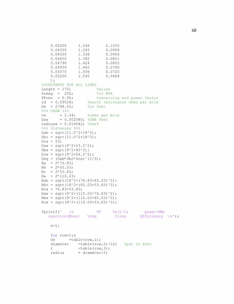
0.04200 1.246 0.1035 0.04350 1.293 0.0969 0.04500 1.338 0.0906 0.04650 1.382 0.0851 0.04790 1.424 0.0803 0.04930 1.465 0.0760 0.05070 1.506 0.0720 0.05200 1.545 0.0684 ]; %CONSTANTS FOR ALL LINES Length = 170; %miles Srmag = 200; %in MVA PFrec = 0.95; %receiving end power factor rd = 0.09528; %earth resistance ohms per mile De = 2788.55; %in feet %%% OHGW %%% rw = 2.44; %ohms per mile Dsw = 0.002085; %GMR feet radiusw = 0.016042; %feeT

%%% Distances %%% Dab = sqrt(11.5^2+18^2); Dbc = sqrt(11.5^2+18^2); Dca = 23; Daw = sqrt(9^2+23.5^2); Dbw = sqrt(9^2+45^2); Dcw = sqrt(9^2+56.5^2); Deq = (Dab*Dbc*Dca)^(1/3); Ha = 2*76.83; Hb = 2*65.03; Hc = 2*53.83; Hw = 2*110.03; Hab = sqrt(18^2+(76.83+65.03)^2); Hbc = sqrt(18^2+(65.03+53.83)^2); Hca = 76.83+53.83; Haw = sqrt(9^2+(110.03+76.83)^2); Hbw = sqrt(9^2+(110.03+65.03)^2); Hcw = sqrt(9^2+(110.03+53.83)^2);

fprintf(' Is PF Vs(L-L) power(MW)

reactive(Mvar) Vreg Ploss Efficiency \n');

n=1;

for row=1:n Ds =table(row,1); diameter =table(row,2)/12; %put in feet r =table(row,3); radius = diameter/2;

69

%%%%%%% Calculating Z and Y %%%%%%%%%

%%%%%%%%%%%%%%%%%%%%%%%%%%%%%%%%%%%% %%% series impedance %%% zaa = r+rd+j*0.12134*log(De/Ds); zbb = zaa; zcc = zaa; zww = rw+rd+j*0.12134*log(De/Dsw); zab = rd+j*0.12134*log(De/Deq); zbc = rd+j*0.12134*log(De/Deq); zca = rd+j*0.12134*log(De/Deq); zaw = rd+j*0.12134*log(De/Daw); zbw = rd+j*0.12134*log(De/Dbw); zcw = rd+j*0.12134*log(De/Dcw); Zs = (1/3)*(zaa+zbb+zcc)-(1/3)*((zaw*zaw+zbw*zbw+zcw*zcw)/zww); Zm = (1/3)*(zab+zbc+zca)-(1/3)*((zaw*zaw+zbw*zbw+zcw*zcw)/zww); z =Zs-Zm; paa = 11.185*log(Ha/radius); %%mile/MF pbb = 11.185*log(Hb/radius); pcc = 11.185*log(Hc/radius); pww = 11.185*log(Hw/radiusw); pab = 11.185*log(Hab/Dab); pbc = 11.185*log(Hbc/Dbc); pca = 11.185*log(Hca/Dca); paw = 11.185*log(Haw/Daw); pbw = 11.185*log(Hbw/Dbw); pcw = 11.185*log(Hcw/Dcw); potential = [ (paa-(paw*paw)/pww) (pab-(paw*pbw)/pww) (pca-

(pcw*paw)/pww) ; (pab-(paw*pbw)/pww) (pbb-(pbw*pbw)/pww) (pbc-(pbw*pcw)/pww) (pca-(pcw*paw)/pww) (pbc-(pbw*pcw)/pww) (pcc-

(pcw*pcw)/pww)]*1000000; capacitan = inv(potential); %% F/mile Ca = capacitan(1,1)-capacitan(1,2)-capacitan(1,3); Cb = capacitan(2,2)-capacitan(2,1)-capacitan(2,3); Cc = capacitan(3,3)-capacitan(3,2)-capacitan(3,1); Cmutual=(1/3)*(capacitan(1,2)+capacitan(2,3)+capacitan(3,1)); Cap = (1/3)*(Ca + Cb + Cc)+(3*Cmutual); y = j*2*pi*60*Cap; %%%% In ohms/mile %%%%%%%%%%%%%%%%%%%%%%%%%%%%%%%%%%%% Z = z * Length; Y = y * Length; %calculating ABCD constants Zc = sqrt(Z/Y); A = cosh(sqrt(Z*Y)); B = Zc*sinh(sqrt(Z*Y)); C = (1/Zc)*sinh(sqrt(Z*Y)); D = A; ABCD = [A B;C D];

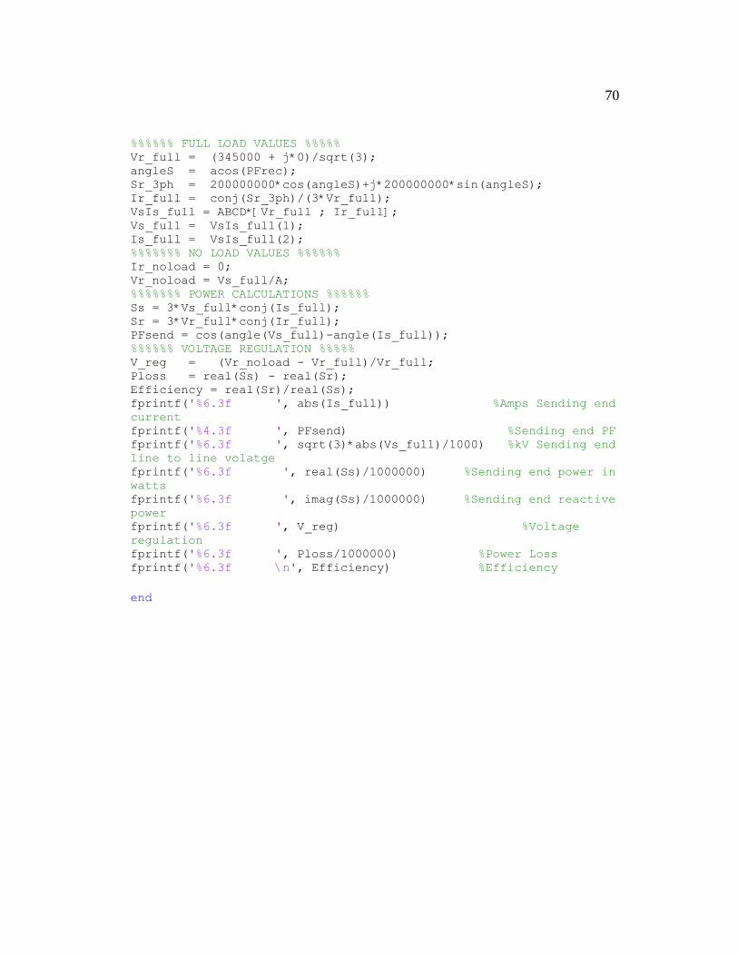
70

%%%%%% FULL LOAD VALUES %%%%% Vr_full = (345000 + j*0)/sqrt(3); angleS = acos(PFrec); Sr_3ph = 200000000*cos(angleS)+j*200000000*sin(angleS); Ir_full = conj(Sr_3ph)/(3*Vr_full); VsIs_full = ABCD*[Vr_full ; Ir_full]; Vs_full = VsIs_full(1); Is_full = VsIs_full(2); %%%%%%% NO LOAD VALUES %%%%%% Ir_noload = 0; Vr_noload = Vs_full/A; %%%%%%% POWER CALCULATIONS %%%%%% Ss = 3*Vs_full*conj(Is_full); Sr = 3*Vr_full*conj(Ir_full); PFsend = cos(angle(Vs_full)-angle(Is_full)); %%%%%% VOLTAGE REGULATION %%%%% V_reg = (Vr_noload - Vr_full)/Vr_full; Ploss = real(Ss) - real(Sr); Efficiency = real(Sr)/real(Ss); fprintf('%6.3f ', abs(Is_full)) %Amps Sending end

current fprintf('%4.3f ', PFsend) %Sending end PF fprintf('%6.3f ', sqrt(3)*abs(Vs_full)/1000) %kV Sending end

line to line volatge fprintf('%6.3f ', real(Ss)/1000000) %Sending end power in

watts fprintf('%6.3f ', imag(Ss)/1000000) %Sending end reactive

power fprintf('%6.3f ', V_reg) %Voltage

regulation fprintf('%6.3f ', Ploss/1000000) %Power Loss fprintf('%6.3f \n', Efficiency) %Efficiency

end

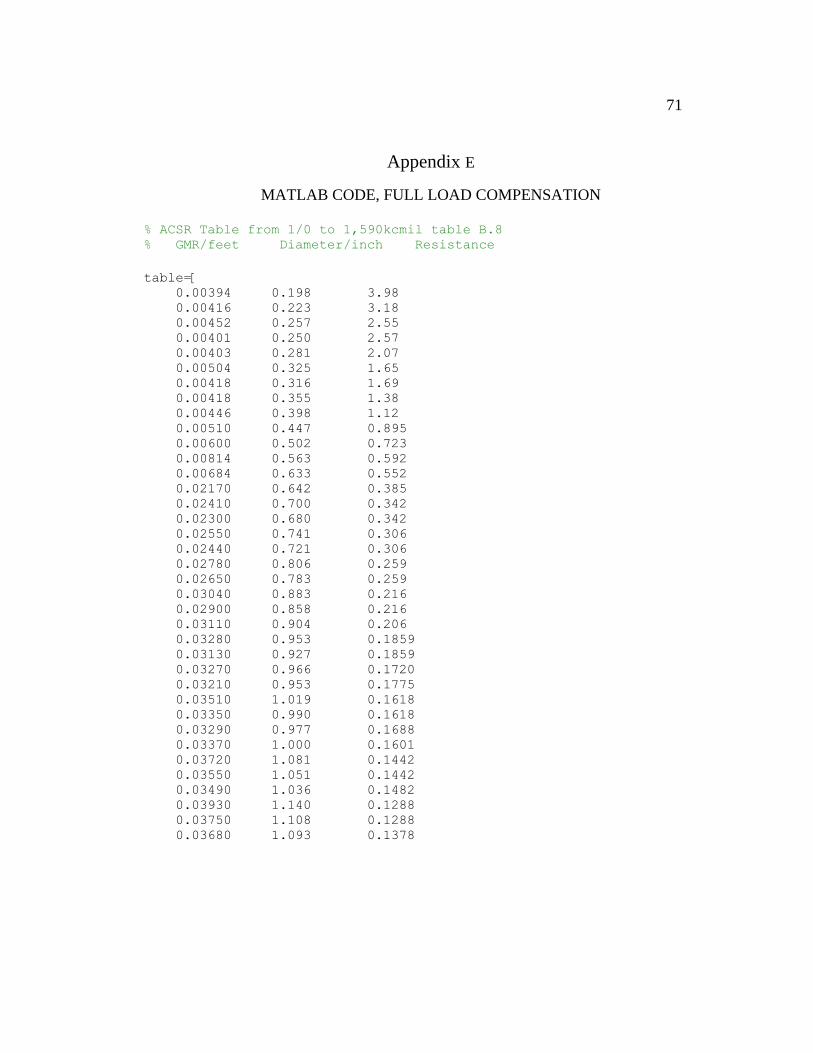
71

Appendix E

MATLAB CODE, FULL LOAD COMPENSATION

% ACSR Table from 1/0 to 1,590kcmil table B.8 % GMR/feet Diameter/inch Resistance

table=[ 0.00394 0.198 3.98 0.00416 0.223 3.18 0.00452 0.257 2.55 0.00401 0.250 2.57 0.00403 0.281 2.07 0.00504 0.325 1.65 0.00418 0.316 1.69 0.00418 0.355 1.38 0.00446 0.398 1.12 0.00510 0.447 0.895 0.00600 0.502 0.723 0.00814 0.563 0.592 0.00684 0.633 0.552 0.02170 0.642 0.385 0.02410 0.700 0.342 0.02300 0.680 0.342 0.02550 0.741 0.306 0.02440 0.721 0.306 0.02780 0.806 0.259 0.02650 0.783 0.259 0.03040 0.883 0.216 0.02900 0.858 0.216 0.03110 0.904 0.206 0.03280 0.953 0.1859 0.03130 0.927 0.1859 0.03270 0.966 0.1720 0.03210 0.953 0.1775 0.03510 1.019 0.1618 0.03350 0.990 0.1618 0.03290 0.977 0.1688 0.03370 1.000 0.1601 0.03720 1.081 0.1442 0.03550 1.051 0.1442 0.03490 1.036 0.1482 0.03930 1.140 0.1288 0.03750 1.108 0.1288 0.03680 1.093 0.1378

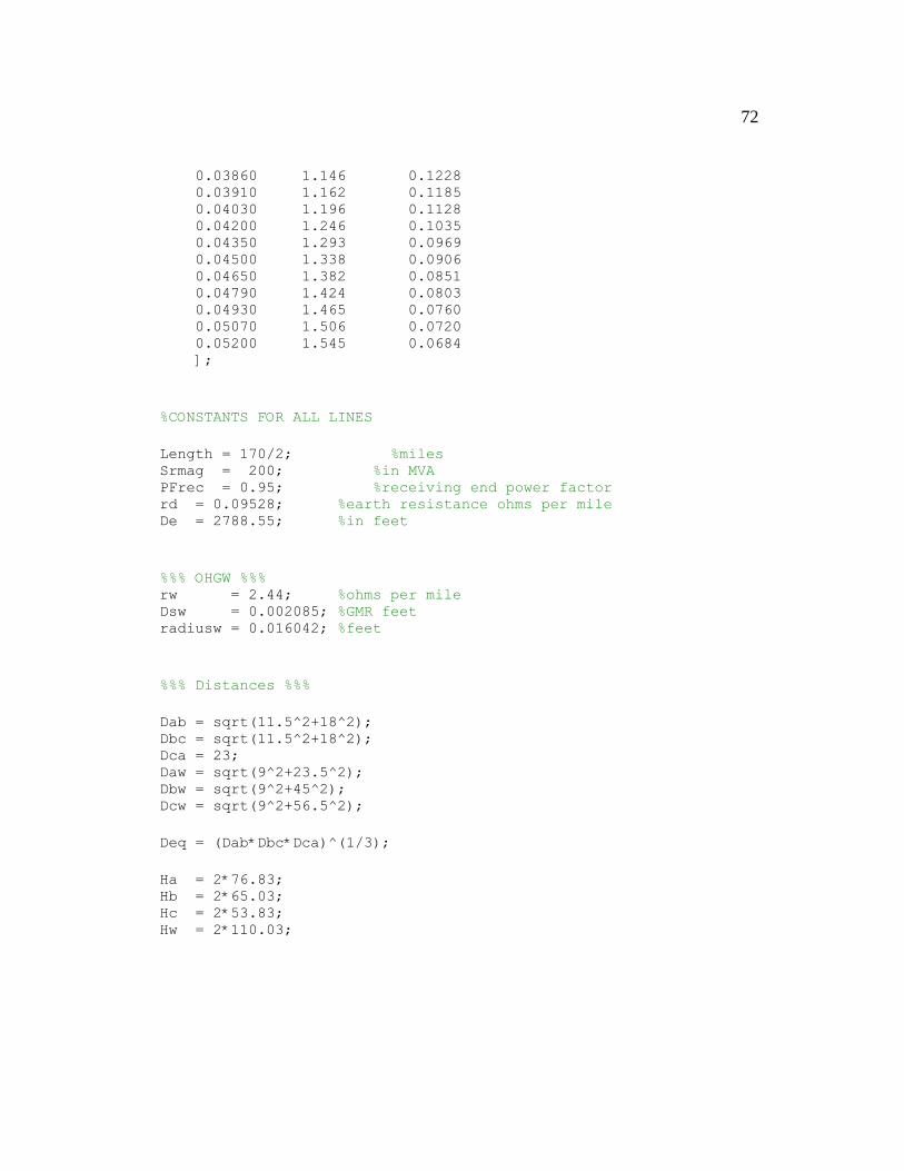
72

0.03860 1.146 0.1228 0.03910 1.162 0.1185 0.04030 1.196 0.1128 0.04200 1.246 0.1035 0.04350 1.293 0.0969 0.04500 1.338 0.0906 0.04650 1.382 0.0851 0.04790 1.424 0.0803 0.04930 1.465 0.0760 0.05070 1.506 0.0720 0.05200 1.545 0.0684 ];

%CONSTANTS FOR ALL LINES

Length = 170/2; %miles Srmag = 200; %in MVA PFrec = 0.95; %receiving end power factor rd = 0.09528; %earth resistance ohms per mile De = 2788.55; %in feet

%%% OHGW %%% rw = 2.44; %ohms per mile Dsw = 0.002085; %GMR feet radiusw = 0.016042; %feet

%%% Distances %%%

Dab = sqrt(11.5^2+18^2); Dbc = sqrt(11.5^2+18^2); Dca = 23; Daw = sqrt(9^2+23.5^2); Dbw = sqrt(9^2+45^2); Dcw = sqrt(9^2+56.5^2);

Deq = (Dab*Dbc*Dca)^(1/3);

Ha = 2*76.83; Hb = 2*65.03; Hc = 2*53.83; Hw = 2*110.03;

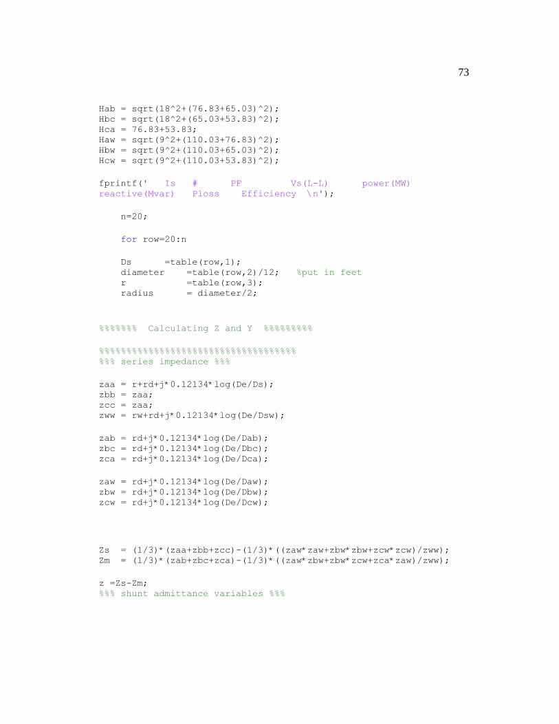
73

Hab = sqrt(18^2+(76.83+65.03)^2); Hbc = sqrt(18^2+(65.03+53.83)^2); Hca = 76.83+53.83; Haw = sqrt(9^2+(110.03+76.83)^2); Hbw = sqrt(9^2+(110.03+65.03)^2); Hcw = sqrt(9^2+(110.03+53.83)^2);

fprintf(' Is # PF Vs(L-L) power(MW)

reactive(Mvar) Ploss Efficiency \n');

n=20;

for row=20:n

Ds =table(row,1); diameter =table(row,2)/12; %put in feet r =table(row,3); radius = diameter/2;


%%%%%%%%%%%%%%%%%%%%%%%%%%%%%%%%%%%% %%% series impedance %%%

zaa = r+rd+j*0.12134*log(De/Ds); zbb = zaa; zcc = zaa; zww = rw+rd+j*0.12134*log(De/Dsw);

zab = rd+j*0.12134*log(De/Dab); zbc = rd+j*0.12134*log(De/Dbc); zca = rd+j*0.12134*log(De/Dca);

zaw = rd+j*0.12134*log(De/Daw); zbw = rd+j*0.12134*log(De/Dbw); zcw = rd+j*0.12134*log(De/Dcw);

Zs = (1/3)*(zaa+zbb+zcc)-(1/3)*((zaw*zaw+zbw*zbw+zcw*zcw)/zww); Zm = (1/3)*(zab+zbc+zca)-(1/3)*((zaw*zbw+zbw*zcw+zca*zaw)/zww);

z =Zs-Zm; %%% shunt admittance variables %%%

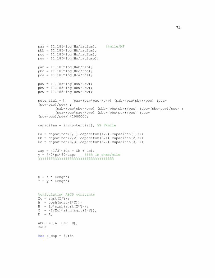
74

paa = 11.185*log(Ha/radius); %%mile/MF pbb = 11.185*log(Hb/radius); pcc = 11.185*log(Hc/radius); pww = 11.185*log(Hw/radiusw);

pab = 11.185*log(Hab/Dab); pbc = 11.185*log(Hbc/Dbc); pca = 11.185*log(Hca/Dca);

paw = 11.185*log(Haw/Daw); pbw = 11.185*log(Hbw/Dbw); pcw = 11.185*log(Hcw/Dcw);

potential = [ (paa-(paw*paw)/pww) (pab-(paw*pbw)/pww) (pca-

(pcw*paw)/pww) ; (pab-(paw*pbw)/pww) (pbb-(pbw*pbw)/pww) (pbc-(pbw*pcw)/pww) ; (pca-(pcw*paw)/pww) (pbc-(pbw*pcw)/pww) (pcc-

(pcw*pcw)/pww)]*1000000;

capacitan = inv(potential); %% F/mile

Ca = capacitan(1,1)-capacitan(1,2)-capacitan(1,3); Cb = capacitan(2,2)-capacitan(2,1)-capacitan(2,3); Cc = capacitan(3,3)-capacitan(3,2)-capacitan(3,1);

Cap = (1/3)*(Ca + Cb + Cc); y = j*2*pi*60*Cap; %%%% In ohms/mile %%%%%%%%%%%%%%%%%%%%%%%%%%%%%%%%%%%%

Z = z * Length; Y = y * Length;

%calculating ABCD constants Zc = sqrt(Z/Y); A = cosh(sqrt(Z*Y)); B = Zc*sinh(sqrt(Z*Y)); C = (1/Zc)*sinh(sqrt(Z*Y)); D = A;

ABCD = [A B;C D]; k=0;

for Z_cap = 84:84

75

ABCD_new = ABCD*[1 -j*Z_cap ;0 1]*ABCD; %%%%%% FULL LOAD VALUES %%%%%

Vr_full = (345000 + j*0)/sqrt(3); angleS = acos(PFrec); Sr_3ph = 200000000*cos(angleS)+j*200000000*sin(angleS);

Ir_full = conj(Sr_3ph)/(3*Vr_full);

VsIs_full = ABCD_new*[Vr_full ; Ir_full];

Vs_full = VsIs_full(1); Is_full = VsIs_full(2);

%%%%%%% POWER CALCULATIONS %%%%%%

Ss = 3*Vs_full*conj(Is_full); Sr = 3*Vr_full*conj(Ir_full); PFsend = cos(angle(Vs_full)-angle(Is_full)); Ploss = real(Ss) - real(Sr);

Efficiency = real(Sr)/real(Ss);

fprintf('%6.3f %d ', abs(Is_full),k) %Amps Sending end

current fprintf('%4.3f ', PFsend) %Sending end PF fprintf('%8.5f ', sqrt(3)*abs(Vs_full)/1000) %kV Sending end

line to line volatge fprintf('%6.3f ', real(Ss)/1000000) %Sending end power in watts fprintf('%6.3f ', imag(Ss)/1000000) %Sending end reactive power fprintf('%6.3f ', Ploss/1000000) %Power loss fprintf('%6.3f ', Efficiency) %Efficiency fprintf('%8.8f \n', 1/(Z_cap*2*pi*60)) %capacitance

k=k+1; end end

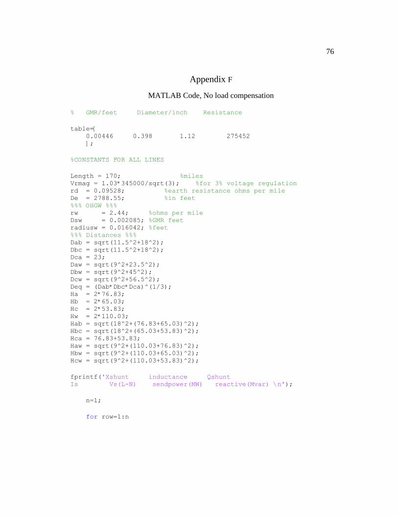
76

Appendix F

MATLAB Code, No load compensation

% GMR/feet Diameter/inch Resistance

table=[ 0.00446 0.398 1.12 275452 ];

%CONSTANTS FOR ALL LINES

Length = 170; %miles Vrmag = 1.03*345000/sqrt(3); %for 3% voltage regulation rd = 0.09528; %earth resistance ohms per mile De = 2788.55; %in feet %%% OHGW %%% rw = 2.44; %ohms per mile Dsw = 0.002085; %GMR feet radiusw = 0.016042; %feet %%% Distances %%% Dab = sqrt(11.5^2+18^2); Dbc = sqrt(11.5^2+18^2); Dca = 23; Daw = sqrt(9^2+23.5^2); Dbw = sqrt(9^2+45^2); Dcw = sqrt(9^2+56.5^2); Deq = (Dab*Dbc*Dca)^(1/3); Ha = 2*76.83; Hb = 2*65.03; Hc = 2*53.83; Hw = 2*110.03; Hab = sqrt(18^2+(76.83+65.03)^2); Hbc = sqrt(18^2+(65.03+53.83)^2); Hca = 76.83+53.83; Haw = sqrt(9^2+(110.03+76.83)^2); Hbw = sqrt(9^2+(110.03+65.03)^2); Hcw = sqrt(9^2+(110.03+53.83)^2);

fprintf('Xshunt inductance Qshunt

Is Vs(L-N) sendpower(MW) reactive(Mvar) \n');

n=1;

for row=1:n

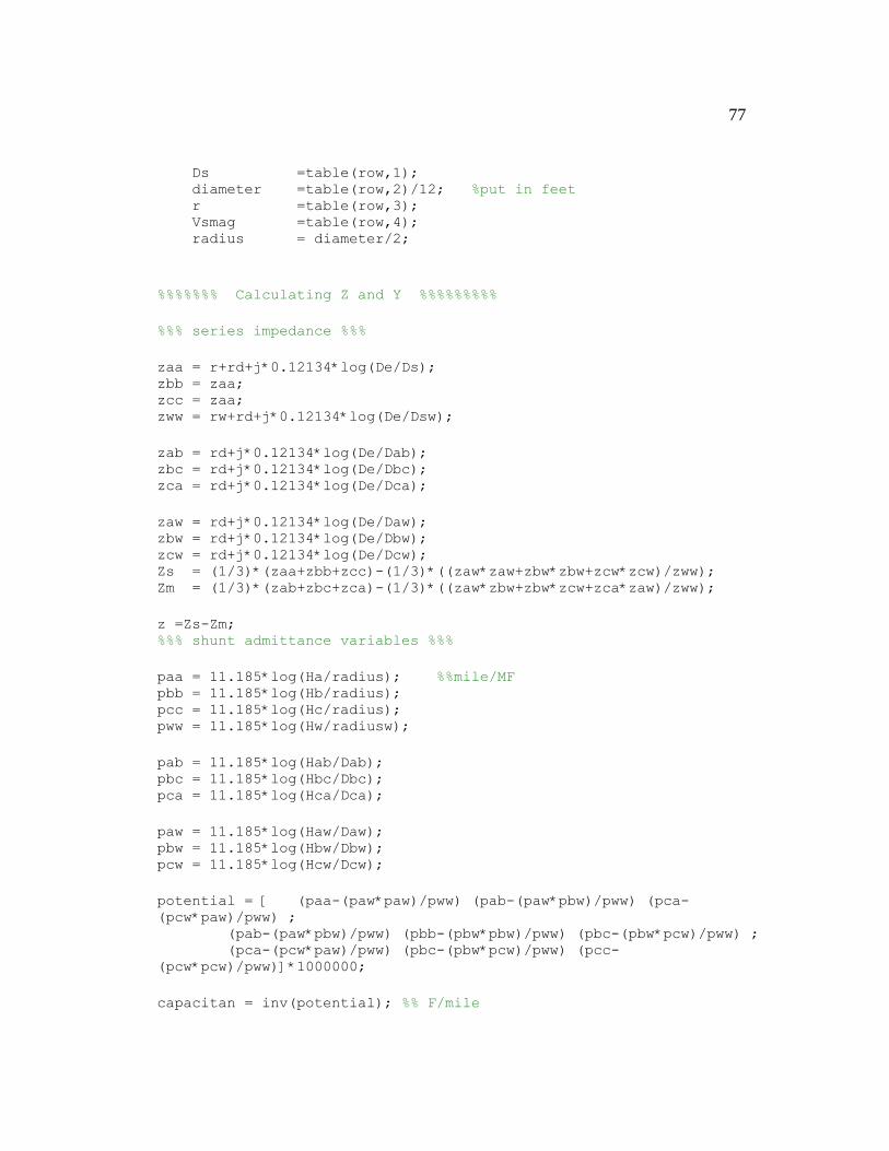
77

Ds =table(row,1); diameter =table(row,2)/12; %put in feet r =table(row,3); Vsmag =table(row,4); radius = diameter/2;


%%% series impedance %%%

zaa = r+rd+j*0.12134*log(De/Ds); zbb = zaa; zcc = zaa; zww = rw+rd+j*0.12134*log(De/Dsw);

zab = rd+j*0.12134*log(De/Dab); zbc = rd+j*0.12134*log(De/Dbc); zca = rd+j*0.12134*log(De/Dca);

zaw = rd+j*0.12134*log(De/Daw); zbw = rd+j*0.12134*log(De/Dbw); zcw = rd+j*0.12134*log(De/Dcw); Zs = (1/3)*(zaa+zbb+zcc)-(1/3)*((zaw*zaw+zbw*zbw+zcw*zcw)/zww); Zm = (1/3)*(zab+zbc+zca)-(1/3)*((zaw*zbw+zbw*zcw+zca*zaw)/zww);

z =Zs-Zm; %%% shunt admittance variables %%%

paa = 11.185*log(Ha/radius); %%mile/MF pbb = 11.185*log(Hb/radius); pcc = 11.185*log(Hc/radius); pww = 11.185*log(Hw/radiusw);

pab = 11.185*log(Hab/Dab); pbc = 11.185*log(Hbc/Dbc); pca = 11.185*log(Hca/Dca);

paw = 11.185*log(Haw/Daw); pbw = 11.185*log(Hbw/Dbw); pcw = 11.185*log(Hcw/Dcw);

potential = [ (paa-(paw*paw)/pww) (pab-(paw*pbw)/pww) (pca-

(pcw*paw)/pww) ; (pab-(paw*pbw)/pww) (pbb-(pbw*pbw)/pww) (pbc-(pbw*pcw)/pww) ; (pca-(pcw*paw)/pww) (pbc-(pbw*pcw)/pww) (pcc-

(pcw*pcw)/pww)]*1000000;

capacitan = inv(potential); %% F/mile

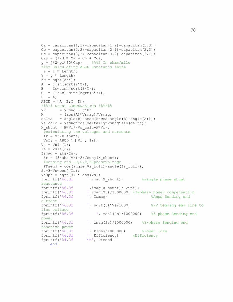
78

Ca = capacitan(1,1)-capacitan(1,2)-capacitan(1,3); Cb = capacitan(2,2)-capacitan(2,1)-capacitan(2,3); Cc = capacitan(3,3)-capacitan(3,2)-capacitan(3,1); Cap = (1/3)*(Ca + Cb + Cc); y = j*2*pi*60*Cap; %%%% In ohms/mile %%%% Calculating ABCD Constants %%%%% Z = z * Length; Y = y * Length; Zc = sqrt(Z/Y); A = cosh(sqrt(Z*Y)); B = Zc*sinh(sqrt(Z*Y)); C = (1/Zc)*sinh(sqrt(Z*Y)); D = A; ABCD = [A B;C D]; %%%%% SHUNT COMPENSATION %%%%%% Vr = Vrmag + j*0; K = (abs(A)*Vrmag)/Vsmag; delta = angle(B)-acos(K*cos(angle(B)-angle(A))); Vs_calc = Vsmag*cos(delta)+j*Vsmag*sin(delta); X_shunt = B*Vr/(Vs_calc-A*Vr); %calculating the voltages and currents Ir = Vr/X_shunt; VsIs = ABCD * [Vr ; Ir]; Vs = VsIs(1); Is = VsIs(2); Ismag = abs(Is); Sr = (3*abs(Vr)^2)/conj(X_shunt); %Sending end PF,S,P,3-phasevoltage PFsend = cos(angle(Vs_full)-angle(Is_full)); Ss=3*Vs*conj(Is); Vs3ph = sqrt(3) * abs(Vs); fprintf('%6.3f ',imag(X_shunt)) %single phase shunt

reactance fprintf('%6.3f ',imag(X_shunt)/(2*pi)) fprintf('%6.3f ',imag(Sr)/1000000) %3-phase power compensation fprintf('%6.3f ', Ismag) %Amps Sending end

current fprintf('%6.3f ', sqrt(3)*Vs/1000) %kV Sending end line to

line voltage fprintf('%6.3f ', real(Ss)/1000000) %3-phase Sending end

power fprintf('%6.3f ', imag(Ss)/1000000) %3-phase Sending end

reactive power fprintf('%6.3f ', Ploss/1000000) %Power loss fprintf('%6.3f ', Efficiency) %Efficiency fprintf('%4.3f \n', PFsend) end

79

BIBLIOGRAPHY

[1] Gonen, T. 2009.Electrical power transmission system engineering analysis and

design, 2nd

ed. Florida: CRC Press.

[2] Gonen, T. 1986.Electrical power distribution system engineering. New York:

McGraw-Hill.

[3] Sadaat, H. 2002.Power system analysis, 2nd

ed. New York: McGraw-Hill.

[4] Granger, J. J. and W. D. Stevenson.1994. Power system analysis. New York:

McGraw-Hill.

[5] SMUD. 1995. UG/OH Conductor sequence impedance study.

[6] Gonen, T. 1988. Modern power system analysis. New York: McGraw-Hill.

Master of Scien ani joupari

Documents

Transcript of Master of Scien ani joupari