MASTER IN ENGINEERING OF STRUCTURES, FOUNDATIONS AND...
119
MASTER IN ENGINEERING OF STRUCTURES, FOUNDATIONS AND MATERIALS MASTER'S THESIS INFLUENCE OF SOIL STIFFNESS ON THE DYNAMIC RESPONSE OF AN OFFSHORE WIND TURBINE Rafael Luque Suárez September 2015
Transcript of MASTER IN ENGINEERING OF STRUCTURES, FOUNDATIONS AND...
MASTER IN ENGINEERING OF STRUCTURES, FOUNDATIONS AND MATERIALS
MASTER'S THESIS
INFLUENCE OF SOIL STIFFNESS ON THE
DYNAMIC RESPONSE OF AN OFFSHORE WIND
TURBINE
Rafael Luque Suárez
September 2015

ABSTRACT
Offshore wind energy industry has experienced a significant growth over the past 15 years,
and it is expected to continue its growth in the coming years. The expansion to increasingly
deep waters and the rise in power and size of the turbines have led to a need for more reliable
and optimized support designs, which requires an extensive knowledge of the behaviour of
these structures. This work focuses on the dynamic response of an offshore wind turbine
founded on a monopile and subjected to wind loading. Different soil properties have been
considered in order to cover the range of stiffness from a very loose to a very dense sand. In
this way, the influence of stiffness on the structure behaviour has been assessed. Static and
dynamic analyses have been carried out by means of a finite element model implemented in
Abaqus. Head displacement and stress at the tower base have been obtained as functions of
soil stiffness, and they have been used to calculate the dynamic amplification that is produced
when the natural frequency of the system soil‐foundation‐tower approaches the load
frequency. Two different approaches of soil modelling have been compared: soil modelled as a
continuum and soil simulated with non linear elastic springs. Finally, a reliability analysis to
assess the probability of resonance has been performed with an analytical model, in which soil
stiffness properties are considered as stochastic variables.
RESUMEN
La industria de la energía eólica marina ha crecido de forma significativa durante los últimos 15
años, y se espera que siga creciendo durante los siguientes. La construcción de torres en aguas
cada vez más profundas y el aumento en potencia y tamaño de las turbinas han creado la
necesidad de diseñar estructuras de soporte cada vez más fiables y optimizadas, lo que
requiere un profundo conocimiento de su comportamiento. Este trabajo se centra en la
respuesta dinámica de una turbina marina con cimentación tipo monopilote y sobre la que
actúa la fuerza del viento. Se han realizado cálculos con distintas propiedades del suelo para
cubrir un rango de rigideces que va desde una arena muy suelta a una muy densa. De este
modo se ha analizado la influencia que tiene la rigidez del suelo en el comportamiento de la
estructura. Se han llevado a cabo análisis estáticos y dinámicos en un modelo de elementos
finitos implementado en Abaqus. El desplazamiento en la cabeza de la torre y la tensión en su
base se han obtenido en función de la rigidez del suelo, y con ellos se ha calculado la
amplificación dinámica producida cuando la frecuencia natural del sistema suelo‐cimentación‐
torre se aproxima a la frecuencia de la carga. Dos diferentes enfoques a la hora de modelizar el
suelo se han comparado: uno utilizando elementos continuos y otro utilizando muelles
elásticos no lineales. Por último, un análisis de fiabilidad se ha llevado a cabo con un modelo
analítico para calcular la probabilidad de resonancia del sistema, en el que se han considerado
las propiedades de rigidez del suelo como variables aleatorias.

TABLE OF CONTENTS
1 INTRODUCTION AND PURPOSE .................................................................................................. 1
2 OFFSHORE WIND TURBINES. OVERVIEW .................................................................................... 3
2.1 TYPOLOGIES ....................................................................................................................................... 3
2.2 LOADS ............................................................................................................................................. 13
2.2.1 Loads on the rotor .............................................................................................................. 13
2.2.2 Loads on the tower ............................................................................................................. 15
2.3 NATURAL FREQUENCY AND MODAL ANALYSIS .......................................................................................... 18
2.4 FAILURE MODES ................................................................................................................................ 21
2.4.1 Limit States ......................................................................................................................... 21
2.4.2 Bearing capacity ................................................................................................................. 23
2.4.3 Examples of failure ............................................................................................................. 25
2.5 ADVANCED DESIGN ASPECTS ................................................................................................................ 28
2.5.1 Soil ‐ structure interaction .................................................................................................. 28
2.5.2 Long term deformations ..................................................................................................... 31
2.5.3 Probabilistic approach ........................................................................................................ 34
2.6 SOLUTIONS AND IMPROVEMENTS ......................................................................................................... 35
2.7 CODES ............................................................................................................................................ 36
3 CASE OF STUDY ........................................................................................................................ 39
3.1 INTRODUCTION ................................................................................................................................. 39
3.2 STRUCTURE AND LOAD PROPERTIES ....................................................................................................... 39
3.3 SOIL PROPERTIES ............................................................................................................................... 40
3.4 MODEL DESCRIPTION ......................................................................................................................... 41
3.5 ANALYSES PERFORMED ....................................................................................................................... 44
4 RESULTS AND DISCUSSION ....................................................................................................... 53
4.1 STATIC LOAD .................................................................................................................................... 53
4.2 FREE OSCILLATION ............................................................................................................................. 54
4.3 FORCED OSCILLATION ......................................................................................................................... 57
4.4 P‐Y AND M‐ CURVES ........................................................................................................................ 66 4.5 MODAL ANALYSIS .............................................................................................................................. 72
4.6 RELIABILITY ANALYSIS ......................................................................................................................... 75
4.6.1 Montecarlo ......................................................................................................................... 76
4.6.2 FORM .................................................................................................................................. 81
5 CONCLUSIONS .......................................................................................................................... 85
6 REFERENCES ............................................................................................................................. 87
A. APPENDIX ................................................................................................................................ 91
I. FREE OSCILLATION. DISPLACEMENTS ..................................................................................................... 91
II. FORCED OSCILLATION. DISPLACEMENTS ................................................................................................. 97
III. FORCED OSCILLATION. STRESSES ......................................................................................................... 103
IV. STATIC EQUIVALENT PLASTIC STRAIN. CASE E=20 MPA ........................................................................... 109
LIST OF TABLES AND FIGURES
Table 3.1: Soil Properties
Table 4.1: Eigen frequencies
Table 4.2: Comparison of both model results
Table 4.3: Adjusted distribution functions to Montecarlo sample
Table 4.4: FORM results
Figure 2.1: Foundation typologies
Figure 2.2: Gravity foundation
Figure 2.3: Installation stages of a suction anchor
Figure 2.4: Tripod foundation
Figure 2.5: Jacket foundation
Figure 2.6: Helical pile
Figure 2.7: Spudcan foundation
Figure 2.8: Floating turbines
Figure 2.9: Vertical axis turbine developed by Vertax
Figure 2.10: Gust factor
Figure 2.11: Effect of wind turbulence
Figure 2.12: Design approaches
Figure 2.13: Cambell diagram
Figure 2.14: Grouted connection
Figure 2.15: Scour hole at Scroby Sands
Figure 2.16: Soil idealization with springs
Figure 2.17: P‐y curves
Figure 2.18: Global foundation stiffness model
Figure 3.1: Global view of the model
Figure 3.2: Dynamic load
Figure 3.3: Equilibrium of forces
Figure 4.1: Horizontal displacement at the head. Static analysis

Figure 4.2: Horizontal displacement at the head. Free oscillation Case E=20 MPa
Figure 4.3: Natural frequency
Figure 4.4: Horizontal displacement at the head. Forced oscillation Case E=10 MPa (f0<)
Figure 4.5: Horizontal displacement at the head. Forced oscillation Case E=20 MPa (f0=)
Figure 4.6: Horizontal displacement at the head. Forced oscillation Case E=40 MPa (f0>)
Figure 4.7: Maximum horizontal displacement at the head. Forced oscillation
Figure 4.8: Dynamic amplification factor
Figure 4.9: Stress contour. Case E=20 MPa
Figure 4.10: Stress history at seabed level. Case E=20 MPa
Figure 4.11: Stress range at seabed level
Figure 4.12: P‐y curve at the base of the tower. Case E=20 MPa
Figure 4.13: M‐ curve at the base of the tower. Case E=20 MPa
Figure 4.14: Plastic equivalent strain. Case E=20 MPa. Increment 9, F=4000 kN
Figure 4.15: Normal forces on the pile. Case E20. Increment 3
Figure 4.16: P‐y curve. Case E=20 MPa. Depth 4.80m
Figure 4.17: Modes of vibration
Figure 4.18: Natural frequency distribution
Figure 4.19: Tested distribution functions

Influence of soil stiffness on the dynamic response of an offshore wind turbine
1
1 Introductionandpurpose
Offshore wind energy industry has grown significantly over the past 15 years, with
Europe leading the way in the development of offshore wind farms, and it will
continue expanding in the coming years. Offshore wind power capacity is expected to
reach a total of 75 GW worldwide by 2020.
The need to build wind turbines in increasingly deep waters and an increment in the
height of the tower to support more powerful turbines are two immediate
consequences of this growth. In this situation, horizontal loads on the structure caused
by wind and waves are dominant factors in its support design. Due to the variable
nature of these loads, a dynamic analysis is required to predict the response of the
structure, both in the short and the long term.
Fatigue damages are critical in these structures and can reduce significantly its life and,
therefore, its profitability. The reason is that offshore structures are subjected to
millions of loading cycles, whose stress amplitude determines the possible occurrence
of damage on the material. This stress amplitude will be higher, due to dynamic
amplification effects, if the excitation frequencies are close to the natural frequency of
the structure. Therefore, the dynamic behaviour of the structure, and particularly its
natural frequency, is a crucial factor in the design of a wind turbine support. This factor
is highly dependent on the stiffness of the foundation and on the characteristics of the
soil.
The influence of the foundation on the dynamic behaviour of an offshore wind turbine
will be analyzed in this document. A total of 9 soil cases with different degree of
stiffness have been covered. Static and dynamic analyses have been performed to
assess the influence of soil stiffness on displacement, natural frequency and stress on
the tower. Two different models have been tested in which the soil has been
implemented in two different ways: as continuous elements in a finite element
simulation, and as springs at the base of the tower. Finally, a reliability analysis has
been performed with an analytical model to obtain the probability of resonance,
considering soil stiffness properties as stochastic variables.
The main objectives to be attained by the present study are as follows:
To review the state of knowledge and summarize the main relevant aspects.
To define the values that geotechnical parameters can take in order to cover
several degrees of stiffness in a granular soil.
1. Introduction and purpose
2
Development in Abaqus of a numerical model of an offshore wind turbine
founded on monopile. Such model is subsequently employed to perform static
and dynamic analyses that illustrate the behaviour of interest.
To assess the influence of soil stiffness on the natural frequency of the
structure.
To obtain the dynamic amplification of the structure in displacements and
stresses as a function of soil stiffness.
To compare the results of two different soil modelling approaches: continuous
elements and springs
To estimate the probability of resonance when soil parameters are considered
as stochastic variables.
A better understanding of the dynamic response of the structure will lead to optimized
designs and more economical foundations; therefore, they could have a significant
economic relevance, as current foundation cost is usually about 35% of the total cost
of the structure. Accurate estimations of the deformability of the foundation will allow
to prevent large displacements and to reduce maintenance operations or reparations
of damage caused by excessive tilt, which will also imply a reduction in the shutdowns
of power generation. Eventually, this will result in an increment of the design life and
profitability of the wind turbine.
Influence of soil stiffness on the dynamic response of an offshore wind turbine
3
2 Offshorewindturbines.Overview
2.1 Typologies
There are different typologies available for offshore wind turbines support. The
foundation has great influence both on the behaviour and cost of the structure,
therefore the choice of its typology is a relevant aspect in the design process,
especially with the increase in size and water depth of the latest turbines. The designer
must take into account, among others, the following factors when choosing a typology:
size of the turbine, water depth, geotechnical characterization of soil, dominant loads,
stiffness, dynamic response, cost and building process.
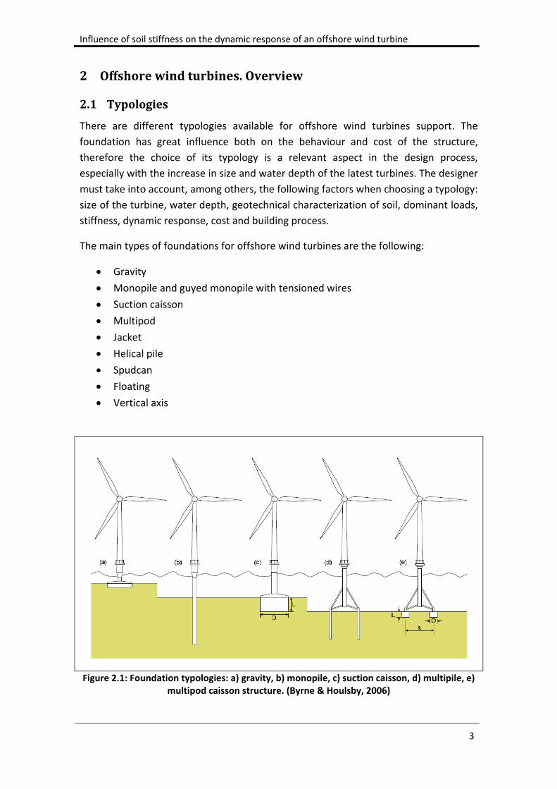
The main types of foundations for offshore wind turbines are the following:
Gravity
Monopile and guyed monopile with tensioned wires
Suction caisson
Multipod
Jacket
Helical pile
Spudcan
Floating
Vertical axis
Figure 2.1: Foundation typologies: a) gravity, b) monopile, c) suction caisson, d) multipile, e) multipod caisson structure. (Byrne & Houlsby, 2006)
2. Offshore Wind turbines. Overview
4
A brief description of these types is made in the following paragraphs.
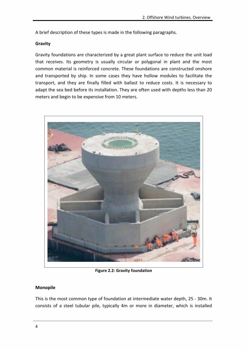
Gravity
Gravity foundations are characterized by a great plant surface to reduce the unit load
that receives. Its geometry is usually circular or polygonal in plant and the most
common material is reinforced concrete. These foundations are constructed onshore
and transported by ship. In some cases they have hollow modules to facilitate the
transport, and they are finally filled with ballast to reduce costs. It is necessary to
adapt the sea bed before its installation. They are often used with depths less than 20
meters and begin to be expensive from 10 meters.
Figure 2.2: Gravity foundation
Monopile
This is the most common type of foundation at intermediate water depth, 25 ‐ 30m. It
consists of a steel tubular pile, typically 4m or more in diameter, which is installed
Influence of soil stiffness on the dynamic response of an offshore wind turbine
5
either by drilling and grouting, or by driving, sometimes by a combination of these two
methods. It reduces the amount of material that a shallow foundation would need at
intermediate depths but the construction process is more complex. Its cost is highly
dependent on the necessary equipment for the installation, as well as the materials.
This typology has been used at Horns Rev, Denmark, and in several wind farms in UK.
The size of monopiles is continuously increasing and giant monopiles designs, in up to
60m water depth, are currently under study. Monopiles of 73.5m length have been
recently fabricated for Siemens' turbines for the German Baltic 2 project, in water
depths of 23 to 44m.
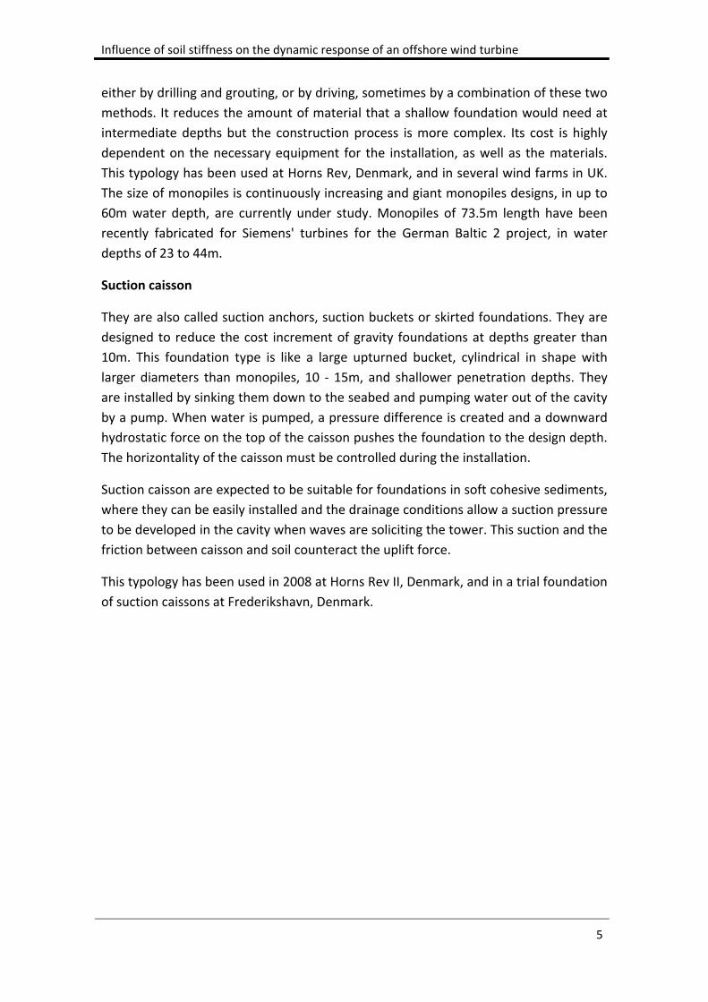
Suction caisson
They are also called suction anchors, suction buckets or skirted foundations. They are
designed to reduce the cost increment of gravity foundations at depths greater than
10m. This foundation type is like a large upturned bucket, cylindrical in shape with
larger diameters than monopiles, 10 ‐ 15m, and shallower penetration depths. They
are installed by sinking them down to the seabed and pumping water out of the cavity
by a pump. When water is pumped, a pressure difference is created and a downward
hydrostatic force on the top of the caisson pushes the foundation to the design depth.
The horizontality of the caisson must be controlled during the installation.
Suction caisson are expected to be suitable for foundations in soft cohesive sediments,
where they can be easily installed and the drainage conditions allow a suction pressure
to be developed in the cavity when waves are soliciting the tower. This suction and the
friction between caisson and soil counteract the uplift force.
This typology has been used in 2008 at Horns Rev II, Denmark, and in a trial foundation
of suction caissons at Frederikshavn, Denmark.
2. Offshore Wind turbines. Overview
6
Figure 2.3: Installation stages of a suction anchor (Malhotra, 2011)
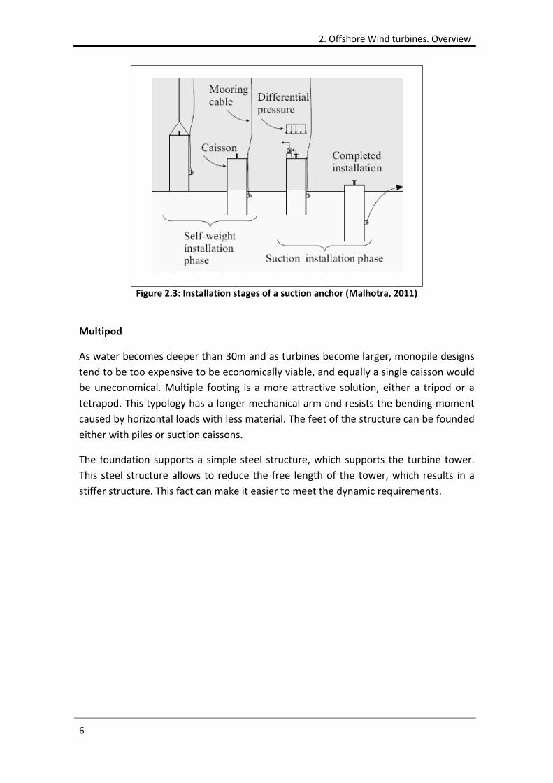
Multipod
As water becomes deeper than 30m and as turbines become larger, monopile designs
tend to be too expensive to be economically viable, and equally a single caisson would
be uneconomical. Multiple footing is a more attractive solution, either a tripod or a
tetrapod. This typology has a longer mechanical arm and resists the bending moment
caused by horizontal loads with less material. The feet of the structure can be founded
either with piles or suction caissons.
The foundation supports a simple steel structure, which supports the turbine tower.
This steel structure allows to reduce the free length of the tower, which results in a
stiffer structure. This fact can make it easier to meet the dynamic requirements.
Influence of soil stiffness on the dynamic response of an offshore wind turbine
7
Figure 2.4: Tripod foundation
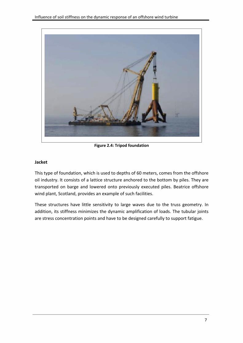
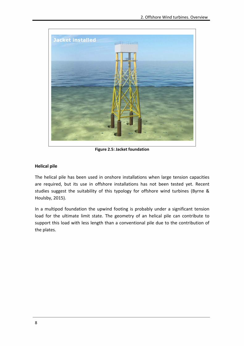
Jacket
This type of foundation, which is used to depths of 60 meters, comes from the offshore
oil industry. It consists of a lattice structure anchored to the bottom by piles. They are
transported on barge and lowered onto previously executed piles. Beatrice offshore
wind plant, Scotland, provides an example of such facilities.
These structures have little sensitivity to large waves due to the truss geometry. In
addition, its stiffness minimizes the dynamic amplification of loads. The tubular joints
are stress concentration points and have to be designed carefully to support fatigue.
2. Offshore Wind turbines. Overview
8
Figure 2.5: Jacket foundation
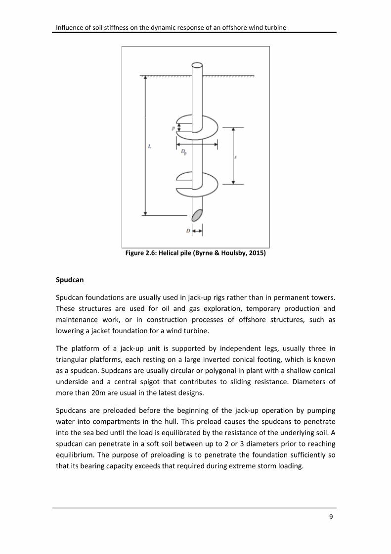
Helical pile
The helical pile has been used in onshore installations when large tension capacities
are required, but its use in offshore installations has not been tested yet. Recent
studies suggest the suitability of this typology for offshore wind turbines (Byrne &
Houlsby, 2015).
In a multipod foundation the upwind footing is probably under a significant tension
load for the ultimate limit state. The geometry of an helical pile can contribute to
support this load with less length than a conventional pile due to the contribution of
the plates.
Influence of soil stiffness on the dynamic response of an offshore wind turbine
9
Figure 2.6: Helical pile (Byrne & Houlsby, 2015)
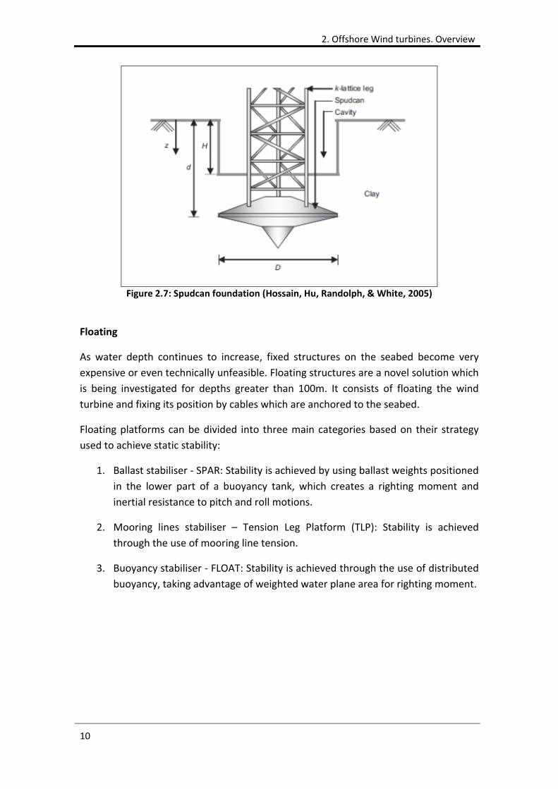
Spudcan
Spudcan foundations are usually used in jack‐up rigs rather than in permanent towers.
These structures are used for oil and gas exploration, temporary production and
maintenance work, or in construction processes of offshore structures, such as
lowering a jacket foundation for a wind turbine.
The platform of a jack‐up unit is supported by independent legs, usually three in
triangular platforms, each resting on a large inverted conical footing, which is known
as a spudcan. Supdcans are usually circular or polygonal in plant with a shallow conical
underside and a central spigot that contributes to sliding resistance. Diameters of
more than 20m are usual in the latest designs.
Spudcans are preloaded before the beginning of the jack‐up operation by pumping
water into compartments in the hull. This preload causes the spudcans to penetrate
into the sea bed until the load is equilibrated by the resistance of the underlying soil. A
spudcan can penetrate in a soft soil between up to 2 or 3 diameters prior to reaching
equilibrium. The purpose of preloading is to penetrate the foundation sufficiently so
that its bearing capacity exceeds that required during extreme storm loading.
2. Offshore Wind turbines. Overview
10
Figure 2.7: Spudcan foundation (Hossain, Hu, Randolph, & White, 2005)
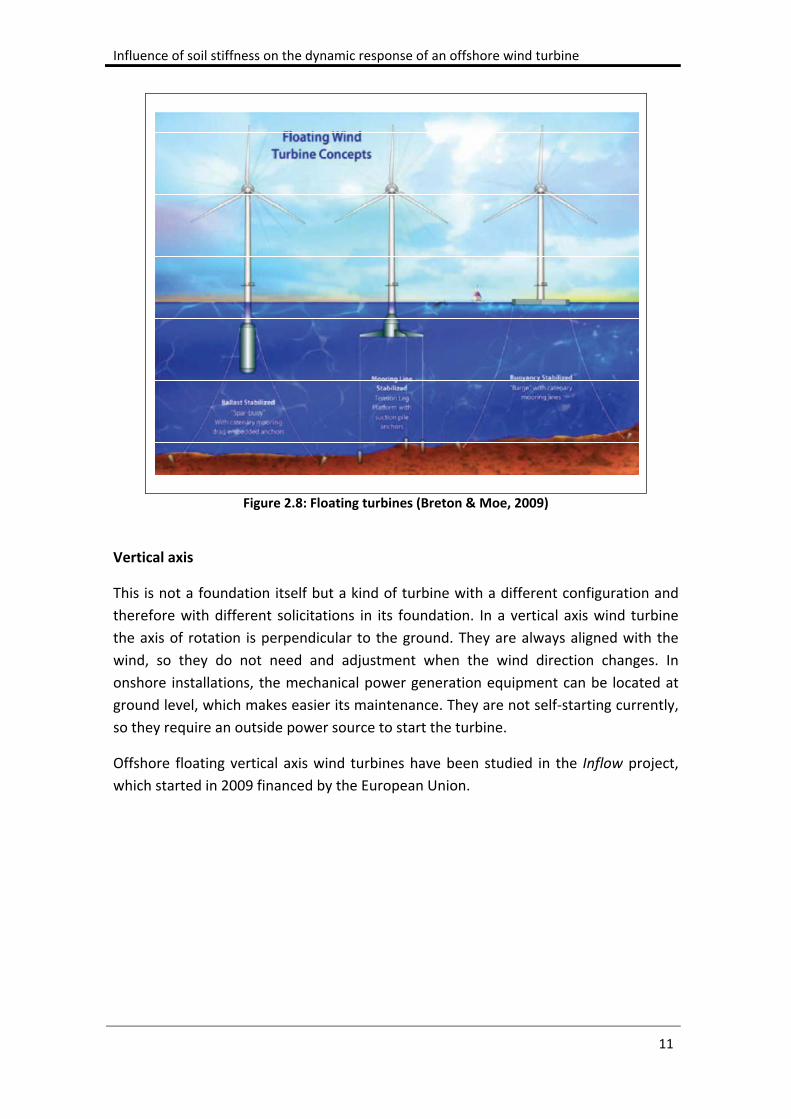
Floating
As water depth continues to increase, fixed structures on the seabed become very
expensive or even technically unfeasible. Floating structures are a novel solution which
is being investigated for depths greater than 100m. It consists of floating the wind
turbine and fixing its position by cables which are anchored to the seabed.
Floating platforms can be divided into three main categories based on their strategy
used to achieve static stability:
1. Ballast stabiliser ‐ SPAR: Stability is achieved by using ballast weights positioned
in the lower part of a buoyancy tank, which creates a righting moment and
inertial resistance to pitch and roll motions.
2. Mooring lines stabiliser – Tension Leg Platform (TLP): Stability is achieved
through the use of mooring line tension.
3. Buoyancy stabiliser ‐ FLOAT: Stability is achieved through the use of distributed
buoyancy, taking advantage of weighted water plane area for righting moment.
Influence of soil stiffness on the dynamic response of an offshore wind turbine
11
Figure 2.8: Floating turbines (Breton & Moe, 2009)
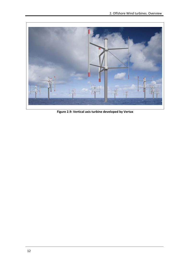
Vertical axis
This is not a foundation itself but a kind of turbine with a different configuration and
therefore with different solicitations in its foundation. In a vertical axis wind turbine
the axis of rotation is perpendicular to the ground. They are always aligned with the
wind, so they do not need and adjustment when the wind direction changes. In
onshore installations, the mechanical power generation equipment can be located at
ground level, which makes easier its maintenance. They are not self‐starting currently,
so they require an outside power source to start the turbine.
Offshore floating vertical axis wind turbines have been studied in the Inflow project,
which started in 2009 financed by the European Union.
2. Offshore Wind turbines. Overview
12
Figure 2.9: Vertical axis turbine developed by Vertax
Influence of soil stiffness on the dynamic response of an offshore wind turbine
13
2.2 Loads
Wind turbines are exposed to very specific actions. Due to the stochastic nature of
wind and waves, loads are variable and difficult to predict. In addition, structural
components and ground are subjected to fatigue, which is a critical state in these
structures. The effect is more critical in large wind turbines: by increasing its size,
complex aeroelastic interactions are created, vibrations and resonances are induced
and they may produce dynamic load amplification. A description of the main loads
which act in the rotor and tower is made in the next paragraphs.
2.2.1 Loadsontherotor
The forces acting on the rotor are attributable to the wind and the weight of the
structure. They can be classified according to their temporary effect in relation to
rotation of the rotor:
Aerodynamic loads of constant winds and centrifugal forces that generate
stationary loads independent of time as long as the rotor turns at constant
speed.
Stationary fields but spatially uneven in the path of the blades, which create
cyclical loads when the rotor is turning:
o The wind flow produces variable loads according to the revolution of
the rotor, since the wind strikes the blades asymmetrically. An
inevitable asymmetry is due to the increase in wind speed with height:
During each revolution, the rotor blades are subjected to higher wind
speeds in the upper part, and therefore to higher loads than the sector
closets to the ground.
o A similar asymmetry is caused by crossed winds which occur with rapid
changes in wind direction.
The inertia forces due to the dead weight of the rotor blades also cause
periodic loads. Furthermore, the gyroscopic loads that occur with rotor
orientation also vary depending on the number of revolutions of the rotor. As
a result of gravity, the blade has a variable bending which changes according to
the angle, thus being an important source of fatigue.
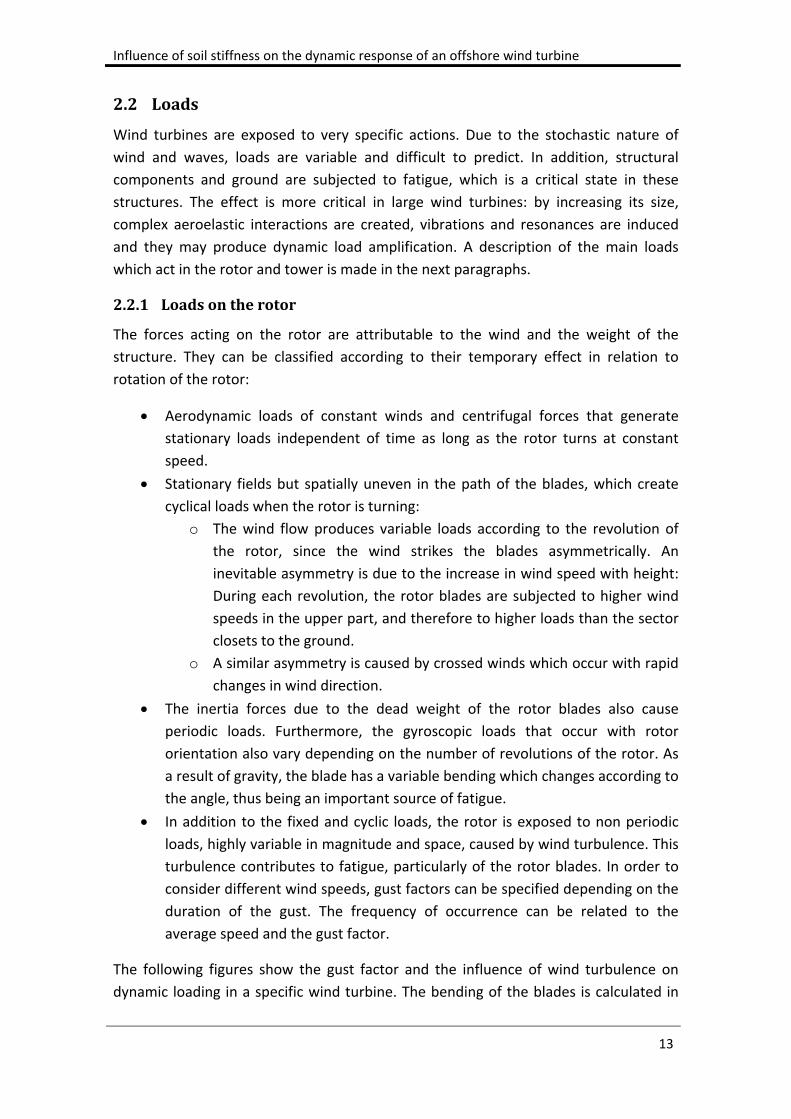
In addition to the fixed and cyclic loads, the rotor is exposed to non periodic
loads, highly variable in magnitude and space, caused by wind turbulence. This
turbulence contributes to fatigue, particularly of the rotor blades. In order to
consider different wind speeds, gust factors can be specified depending on the
duration of the gust. The frequency of occurrence can be related to the
average speed and the gust factor.
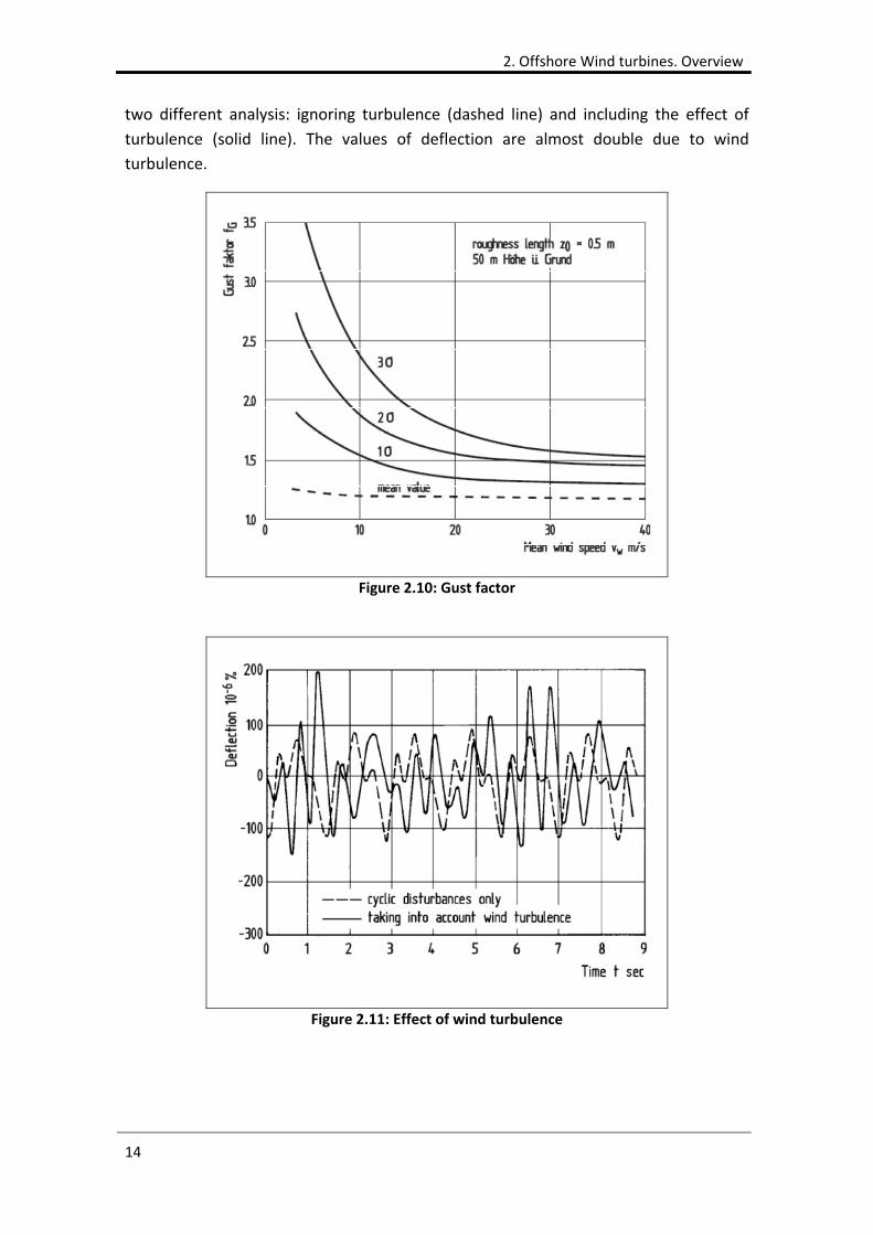
The following figures show the gust factor and the influence of wind turbulence on
dynamic loading in a specific wind turbine. The bending of the blades is calculated in
2. Offshore Wind turbines. Overview
14
two different analysis: ignoring turbulence (dashed line) and including the effect of
turbulence (solid line). The values of deflection are almost double due to wind
turbulence.
Figure 2.10: Gust factor
Figure 2.11: Effect of wind turbulence
Influence of soil stiffness on the dynamic response of an offshore wind turbine
15
2.2.2 Loadsonthetower
The forces on the shaft of the turbine are due to environmental actions. Two
conditions can be distinguished depending of their probability of occurrence: service
conditions, which are expected to occur often, and extreme conditions, which occur
rarely during the life of the structure. The design loads of the structure will be different
in each condition. A description of the main loads acting on the tower of an offshore
wind turbine is made in the following paragraphs.
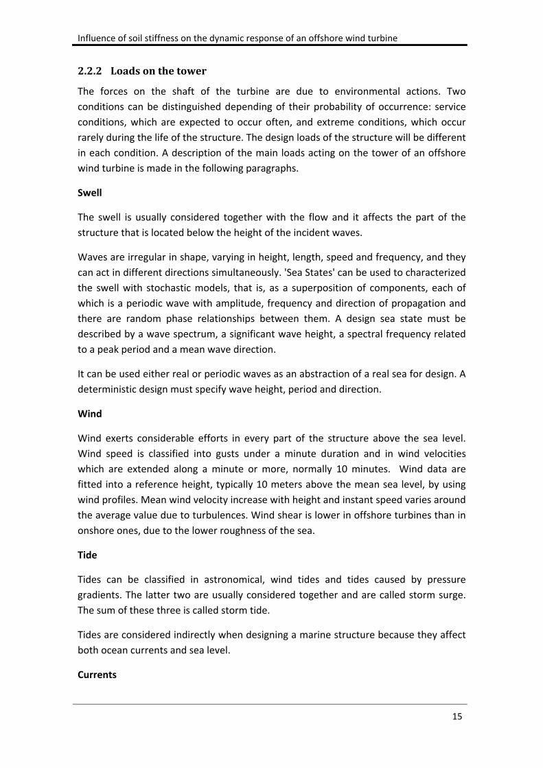
Swell
The swell is usually considered together with the flow and it affects the part of the
structure that is located below the height of the incident waves.
Waves are irregular in shape, varying in height, length, speed and frequency, and they
can act in different directions simultaneously. 'Sea States' can be used to characterized
the swell with stochastic models, that is, as a superposition of components, each of
which is a periodic wave with amplitude, frequency and direction of propagation and
there are random phase relationships between them. A design sea state must be
described by a wave spectrum, a significant wave height, a spectral frequency related
to a peak period and a mean wave direction.
It can be used either real or periodic waves as an abstraction of a real sea for design. A
deterministic design must specify wave height, period and direction.
Wind
Wind exerts considerable efforts in every part of the structure above the sea level.
Wind speed is classified into gusts under a minute duration and in wind velocities
which are extended along a minute or more, normally 10 minutes. Wind data are
fitted into a reference height, typically 10 meters above the mean sea level, by using
wind profiles. Mean wind velocity increase with height and instant speed varies around
the average value due to turbulences. Wind shear is lower in offshore turbines than in
onshore ones, due to the lower roughness of the sea.
Tide
Tides can be classified in astronomical, wind tides and tides caused by pressure
gradients. The latter two are usually considered together and are called storm surge.
The sum of these three is called storm tide.
Tides are considered indirectly when designing a marine structure because they affect
both ocean currents and sea level.
Currents
2. Offshore Wind turbines. Overview
16
Although currents are usually variable in space and time, they are generally considered
as a flow with constant speed and direction, varying only with depth. There are four
types of currents:
Wind generated currents
Tidal currents
Subsurface currents
Near shore currents
Ice
When wind turbines are projected in an area where water can freeze or where ice can
come adrift, this factor must be considered and it must be taken into account aspects
such as geometry and nature of the ice, its concentration and distribution, type of ice,
mechanical properties, velocity, direction of drift and the probability of encountering
icebergs.
Other conditions
It is essential to collect any additional environmental information available, as it would
be the salinity of water, seismicity of the area, temperature and so on. These are
factors that may be involved in some aspects of the design.
2.2.2.1 Morrisonequation
The dynamic wave analysis is indicated when the foundation of the wind turbine
allows large movements of the structure with respect to the sea, as it is the case of a
floating structure, or when loads are close to the natural frequency of the structure.
Moreover, the natural frequency of the structure has to be fitted between the
frequency of the rotor, 1P, and the frequency of the blades, 2P or 3P, and sometimes
wave frequencies are in this interval and therefore could be near the natural frequency
of the structure. This is a determining factor in the fatigue analysis of the structure
because the stress amplitude of each cycle is larger if the natural and excitation
frequencies are similar.
The force caused by waves on the shaft of the turbine is time dependent and can be
obtained with the Morrison equation:
Where:
Influence of soil stiffness on the dynamic response of an offshore wind turbine
17
, ′: Components of the velocities of tower and water due to currents and waves
normal to the cylinder axis.
, ′: Components of the accelerations of tower and water normal to the cylinder axis.
: Water density
D: Effective diameter, including marine growth.
Cd: Drag coefficient
Cm: Inertia coefficient
d, (t): Limit values of water and wave depth integration
2.2.2.2 Characterizationofwindload
Wind actions on the structure are time dependent and cause pressure acting on the
surface and producing normal forces. The overall response of the structure to wind can
be considered as a superposition of a quasi‐static 'background' component and a
'resonant' component due to the excitation of the natural frequencies. In the turbines,
the resonant effect of wind is given by the rotation of the blades. The symmetry of the
support structure allows not to take into account directionality, however, according to
UNE ENV1991‐2‐4, the following instability dynamic phenomena must be considered:
vortex shedding, galloping, flutter, divergence, interference galloping.
The basic wind pressure is defined by the following equation:
Where:
a: Air density
Cs: Shape coefficient
Vt,z: Mean wind velocity during a period T and z meters over the mean sea level
Vertical angle between wind direction and cylindrical axis.
2. Offshore Wind turbines. Overview
18
2.3 Naturalfrequencyandmodalanalysis
The response of an offshore wind turbine to wind and wave loads is highly dependent
on the natural frequency of the system hub‐tower‐foundation, due to the dynamic
nature of these loads and the slenderness of the system. The natural frequency will
determine the stress and strain amplitudes produced by loading cycles, which in turn
determine the fatigue failure of the structure. Therefore, an accurate estimation of this
parameter is essential to assess the working life of a wind turbine.
In order to avoid resonance, the natural frequency of the system and the main load
frequency must be far enough from each other. The most repetitive load of a wind
turbine is that generated by mass imbalances in the rotor, whose frequency is usually
called '1P'. The shadowing effect of wind is also related to this frequency: each time a
blade passes the tower, the wind force stop pushing directly on it. The frequency of
this effect is n*P, 'n' being the number of blades in the turbine, which is 3 in most
cases. Therefore, the natural frequency of the tower must be far from 1P and 3P.
The rotor of modern wind turbines does not operate at constant velocity but in a range
of different velocities, therefore, there are two ranges of operating frequencies around
1P and 3P. The natural frequency of the tower cannot be in any of these two ranges.
There are three classical approaches to classify the design of a wind turbine structure
according to its natural frequency, the frequency 'P' of the rotor and frequency '3P' of
the blades:
Soft‐Soft: The natural frequency is less than '1P'. This implies a high flexibility of the structure. Furthermore, the frequency of waves is usually within this range, which can lead to resonance.
Soft‐Stiff: The tower frequency lies between 1P and 3P. This is the most common design.
Stiff‐Stiff: The tower frequency is higher than the passing blade frequency 3P. This leads to very stiff and therefore expensive foundations.
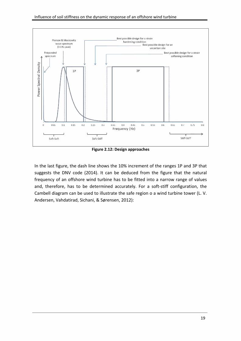
The next figure illustrates the possible design approaches depending on the value of
the natural frequency (Bhattacharya, 2014). The figure also refers to possible long
term changes in the natural frequency caused by soil hardening or softening under
cyclic loading. Although these considerations are outside the scope of this study, it
basically means that if the soil has a hardening trend, the natural frequency of the
system will increase with time, therefore, its design value should be lower. In the case
of softening, the design value of the natural frequency should be higher and it will
decrease with time.
Influence of soil stiffness on the dynamic response of an offshore wind turbine
19
Figure 2.12: Design approaches
In the last figure, the dash line shows the 10% increment of the ranges 1P and 3P that
suggests the DNV code (2014). It can be deduced from the figure that the natural
frequency of an offshore wind turbine has to be fitted into a narrow range of values
and, therefore, has to be determined accurately. For a soft‐stiff configuration, the
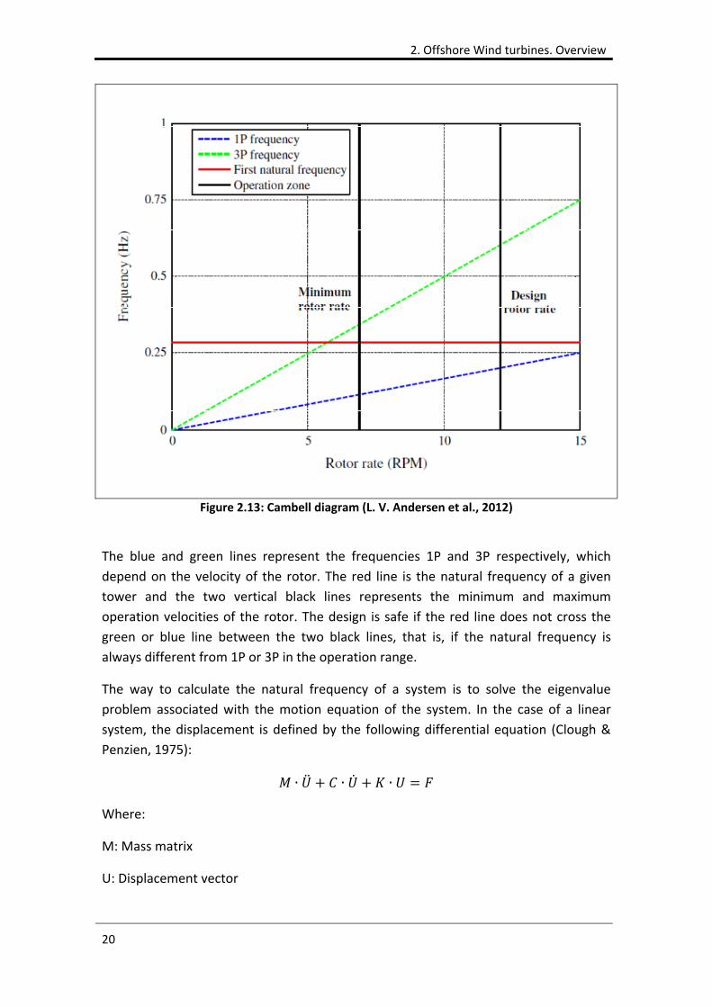
Cambell diagram can be used to illustrate the safe region o a wind turbine tower (L. V.
Andersen, Vahdatirad, Sichani, & Sørensen, 2012):
2. Offshore Wind turbines. Overview
20
Figure 2.13: Cambell diagram (L. V. Andersen et al., 2012)
The blue and green lines represent the frequencies 1P and 3P respectively, which
depend on the velocity of the rotor. The red line is the natural frequency of a given
tower and the two vertical black lines represents the minimum and maximum
operation velocities of the rotor. The design is safe if the red line does not cross the
green or blue line between the two black lines, that is, if the natural frequency is
always different from 1P or 3P in the operation range.
The way to calculate the natural frequency of a system is to solve the eigenvalue
problem associated with the motion equation of the system. In the case of a linear
system, the displacement is defined by the following differential equation (Clough &
Penzien, 1975):
∙ ∙ ∙
Where:
M: Mass matrix
U: Displacement vector
Influence of soil stiffness on the dynamic response of an offshore wind turbine
21
C: Damping matrix
K: Stiffness matrix
F: External forces vector
In the particular case of zero damping, the free vibration problem considering the
common hypothesis of an harmonic solution, U=A*sin(t+), can be expressed as follows:
∙ ∙ ∙
∙ ∙1∙
The equation above is the eigenvalue problem for the matrix K‐1*M. For a n‐degree of
freedoms system, there are n number of modes, each one with a frequency of
vibration. The lowest frequency is called the natural frequency of the structure. If the
system is linear, which implies that all elements of the stiffness matrix are constant,
and the stiffness matrix is symmetrical, the solution of the forced vibration problem
can be expressed as a superposition of the vibration modes:
∑ ∅ ∗ for i =1,...n
Where:
∅ : Mode shape coordinate representing the position of the i‐mass in the j‐node.
: Generalized coordinate representing the variation of the response in mode j
with time.
When the system is very big, the solution obtained by modal superposition stops to be
reliable. In most common structures, the solution can be expressed accurately enough
with a few modes of vibration.
2.4 Failuremodes
2.4.1 LimitStates
The main limit states which have to be analyzed in an offshore wind turbine are the
following:
Ultimate Limit State (ULS).
Fatigue Limit State (FLS).
Accidental Limit State (ALS).
Serviceability Limit State (SLS).
2. Offshore Wind turbines. Overview
22
The Ultimate Limit State refers to the capacity of the foundation to resist the
maximum load. It is necessary to analyze the critical combination of moment, lateral
and axial load, which gives the failure envelope of the foundation. Although it is
necessary to study each case, the maximum load is usually caused by waves during a
storm. In this situation the power production is stopped in order to reduce the
maximum load caused by wind. Therefore the wind forces on blades are of minor
importance in this state. The DNV gives the following examples of ULS failures:
Loss of structural resistance (excessive yielding and buckling).
Failure of components due to brittle fracture.
Loss of static equilibrium of the structure, or of a part of the structure,
considered as a rigid body, e.g. overturning or capsizing.
Failure of critical components of the structure caused by exceeding the
ultimate resistance (which in some cases is reduced due to repetitive loading)
or the ultimate deformation of the components.
Transformation of the structure into a mechanism (collapse or excessive
deformation).
The Fatigue Limit State is the failure due to the effect of cyclic loading. Most loads that
excite wind tower turbines are cyclic, such as rotation of blades, wind or waves; so the
structure is affected by repetitive cycles of load. The repetition of these cycles, which
can be about N=108 throughout the life of a wind turbine, reduces the resistance of the
structure. The damage caused by fatigue is highly dependent on stress amplitude,
which is affected by the natural frequency of the system tower‐foundation. If the
excitation frequency is close to the natural frequency of the structure, the stress
amplitude of the load cycles is larger, therefore it is necessary to take into account the
dynamics effects. The stiffness of the foundation plays a fundamental role in the
mitigation or amplification of the dynamics effects.
The Accidental Limit State corresponds to maximum load‐carrying capacity for
accidental loads or post‐accidental integrity for damaged structures. Some examples of
ALS are the following:
Structural damage caused by accidental loads.
Ultimate resistance of damaged structures.
Loss of structural integrity after local damage.
The Serviceability Limit State gives the tolerance criteria applicable to normal use. A
critical aspect in this state is the tilt at the hub level over the life of the structure. To
obtain it, it is necessary to calculate with a certain degree of reliability the settlement
and inclination of the foundation. Usually, the tilt criterion is very exigent and leads to
a design with a very stiff foundation, which increases its cost, this being about 35% of
Influence of soil stiffness on the dynamic response of an offshore wind turbine
23
the cost of the structure. A full understanding of the behaviour of the foundation is
necessary in order to optimize the design of the system. The DNV code gives the
following examples of SLS:
Deflections that may alter the effect of the acting forces.
Deformations that may change the distribution of loads between supported
rigid objects and the supporting structure.
Excessive vibrations producing discomfort or affecting non‐structural
components.
Motions that exceed the limitation of equipment.
Differential settlements of foundations soils causing intolerable tilt of the wind
turbine.
Temperature‐induced deformations.
Taking into account the previous Limit States, the following design aspects have to be
considered in the design of a wind tower foundation:
Capacity. Critical in ULS and ALS.
Stiffness and deformation. Critical in SLS and FLS.
Long term repetition of cycles, up to N=108. Critical in FSL.
2.4.2 Bearingcapacity
The most critical aspect in the Ultimate and Accidental Limit States is the bearing
capacity of the foundation, especially in shallow foundations. They have some specific
particularities that must be taken into account in the design. In the following
paragraphs, some of these aspects will be described briefly.
In general, there are two situations that have to be studied depending on the soil
conditions:
Undrained clays
Fully or partially drained conditions in sands (depends on permeability)
The bearing capacity and failure envelopes for combined loading of a skirted
foundation, considering that shear strength varies with depth, have been studied by
Gourvenec and Randolph (2003). They concluded that in the plane V:H, with M=0, the
shape of the failure envelope is independent of the foundation geometry or the
degree of non homogeneity. In the plane V:M, with H=0, they found a simple power
law relationship with the non homogeneity ratio. However, in the plane H:M, where
the failure envelope is asymmetric, they did not find a simple relationship.
An undrained failure envelope was studied lately by some of these authors,
considering general 3D loading and shear strength heterogeneity (Gourvenec &
2. Offshore Wind turbines. Overview
24
Barnett, 2011). The authors proposed closed form expressions to predict the ultimate
limit states V‐H‐M that provides the apex points of the failure envelope and the shape
of the normalized envelope. The size and shape of the envelope depends on load
combination, embedment ratio and degree of soil strength heterogeneity.
A six degree of freedom model based on work hardening plasticity models has been
developed to study the response of shallow foundations to general loading (Bienen,
Byrne, Houlsby, & Cassidy, 2006). This model provides the yield surface, plastic
potential expressions, a hardening law and the elastic stiffness derived from unload‐
reload loops of load.
Andersen (2009) studied the behaviour of soils under cyclic loading in both offshore
and onshore structures. He observed that the cyclic shear strength and the failure
mode under cyclic loading depend strongly on the strength path and the combination
of average and cyclic shear stresses. Andersen concluded that the foundation capacity
under cyclic loading can be determined on the basis of cyclic shear strength
determined in laboratory tests.
For a suction caisson there are two states which must be analyzed, each one with
different load configuration:
Installation
Service
In the installation stage it is necessary to estimate the self weight penetration of the
caisson and the suction required. These two parameters can be calculated from CPT
data and caisson geometry by using a model based on measured data (Houlsby, Ibsen,
& Byrne, 2005). The horizontality of the caisson during the installation can be
controlled by dividing the caisson in two section and measuring the pressure in each
one.
The cavity depth in spudcan foundations during the penetration stage is a critical
parameter and can trigger a soil flow failure. The cavity depth is limited then by this
failure, which can be more restrictive than the wall failure incorporated in the
guidelines, that is, collapse of the vertical sides of the soil (Hossain et al., 2005).
Houlsby et al. (2005) carried out laboratory model testing, centrifuge model testing,
field trials at reduced scale and a full scale installation of an offshore wind tower. From
these experiments they developed plasticity based models to represent the behaviour
of monopod and tetrapod caisson foundations under cyclic loading. They concluded
that stiffness and fatigue are as important for turbine design as ultimate capacity. They
also observed a stiffness reduction and an increase in hysteresis when the load
amplitude, either vertical or moment, increases.
Influence of soil stiffness on the dynamic response of an offshore wind turbine
25
In multipod caisson foundations the uplift capacity is a relevant parameter. A reliable
understanding of the tensile capacity can reduce the separation between foots and
therefore the size of the foundation. Centrifuge tests conducted under undrained
conditions have been carried out to study the relationship between peak uplift
resistance, embedment ratio, state of the skirt‐soil interface, displacement and loss of
suction (Mana, Gourvenec, & Randolph, 2013). They concluded that peak undrained
uplift resistance is mobilized at displacements between 2% and 5% of the foundation
diameter, increasing with the embedment ratio.
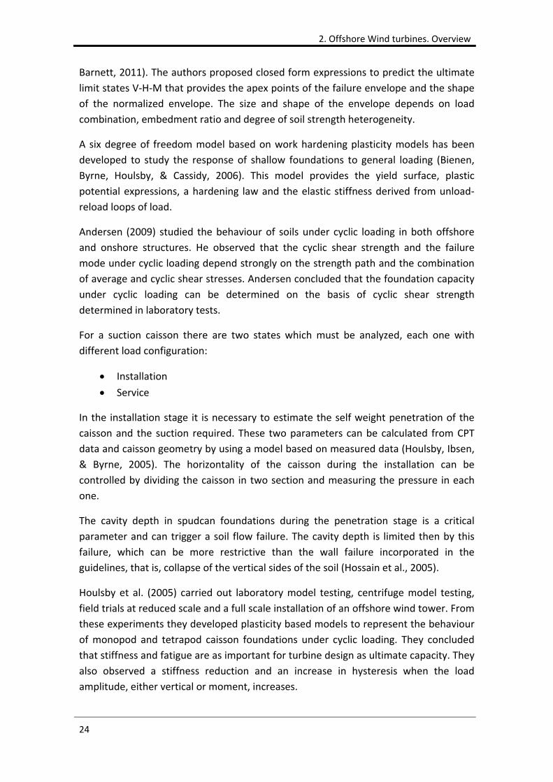
2.4.3 Examplesoffailure
A failure detected in several offshore wind turbines with monopile foundation is the
displacement of the transition piece. This piece is usually located at sea water level,
between the turbine steel tower and the monopile. The link between the transition
piece and the monopile is called the grouted connection, which is showed in the next
figure:
Figure 2.14: Grouted connection (Löhning, Voßbeck, & Kelm, 2013)
A failure in the grouted connection has been detected in hundreds of offshore wind
turbines all over Europe, several years after construction. The transition piece slid
several centimetres and this settlement had to be stopped by temporary brackets
2. Offshore Wind turbines. Overview
26
(Löhning et al., 2013). The repetition of cycles of bending moment is believed to be
one of the main reasons of this failure. The stress amplitude of these cycles is a critical
parameter to analyze the fatigue failure of the grouted connection.
A very restrictive parameter in a wind turbine is the tilt of the tower. Predictions show
that cyclic displacements could be two to five times the static single load values,
depending on the pile size, stiffness and depth. Therefore, to estimate the tilt of the
tower along its whole life it is necessary to analyze the long term displacement under
cyclic loading. The usual limit criteria for the tilt is 0.25°, although there is little to no
monitoring of lateral movement in existing turbines to justify this criterion. A rational
analysis of the operational limits of the turbine could lead to a less restrictive tilt limit
and therefore to a reduction in the foundation size (Golightly, 2014).
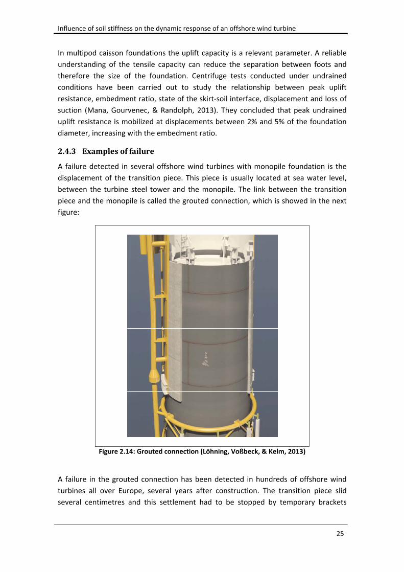
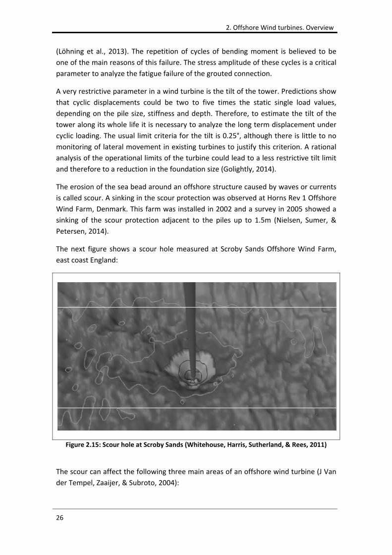
The erosion of the sea bead around an offshore structure caused by waves or currents
is called scour. A sinking in the scour protection was observed at Horns Rev 1 Offshore
Wind Farm, Denmark. This farm was installed in 2002 and a survey in 2005 showed a
sinking of the scour protection adjacent to the piles up to 1.5m (Nielsen, Sumer, &
Petersen, 2014).
The next figure shows a scour hole measured at Scroby Sands Offshore Wind Farm,
east coast England:
Figure 2.15: Scour hole at Scroby Sands (Whitehouse, Harris, Sutherland, & Rees, 2011)
The scour can affect the following three main areas of an offshore wind turbine (J Van
der Tempel, Zaaijer, & Subroto, 2004):
Influence of soil stiffness on the dynamic response of an offshore wind turbine
27
Foundation length
Natural frequency
J‐tube
When scour occurs, the effective length of the foundation decreases. The resistance of
the upper layers of soil is removed and the overburden pressure around the lower part
of the pile is reduced. Therefore, scour can affect the bearing capacity of the pile.
Scour has also impact on the natural frequency of the structure, which decreases with
an increasing scour depth. This reduction in the natural frequency implies a reduction
in the stiffness, which can affect the stress range and the fatigue damage.
The J‐tube is used to support the power cable from the turbine to the seabed. When
scour occurs, the J‐tube could be free spanning over the scour hole, which could
damage the power cable.
In deep waters the wall thickness of a monopile is conditioned by the buckling failure.
De Vries and Krolis (2007) have studied the buckling of a section at the mud line in
several offshore wind turbines in water depths ranging from 20 to 50m. They
concluded that the mass of the support structure increases dramatically with
increasing water depth. A ratio of the wall thickness and the diameter of the monopile
of 1:80 is a good initial estimate.
A possible failure in a multipod foundation is the uplift of one of the legs due to a
lateral load. In a monopod foundation, the uplift capacity is also mobilized in part of
the section to resist a strong bending moment. In the particular case of a skirted
foundation, a negative excess pore pressure can be generated between the foundation
top plate and the confined soil plug during undrained uplift, allowing reverse end
bearing capacity to be mobilized. A possible failure in this situation is the loss of
suction under the top plate. In order to avoid this, it is necessary to determine the
minimum skirt depth to foundation diameter embedment ratio required to generate
negative excess pore pressure under the top cap. It is also important to determine
over what duration the negative excess pore pressure can be sustained (Mana,
Gourvenec, Randolph, & Hossain, 2012).
In the case of spudcan foundations, most codes consider the instability of the cavity
walls during the penetration stage, which limits the depth of the foundation. However,
a more critical failure during the penetration stage is the soil flow failure (Hossain et
al., 2005). The soil back flow into the cavity can occur due to:
Plastic flow around the spudcan edge
Collapse of the vertical cavity walls into the hole
A combination of these
2. Offshore Wind turbines. Overview
28
Liquefaction is a phenomenon that produces a drastic reduction in the effective
pressure of the soil due to an increase in the pore pressure. De Groot, Kudella, Meijers
and Oumeraci (2006) studied the phenomenon of liquefaction in structures subjected
to wave loads. They considered four types of failures:
Liquefaction flow failure
Stepwise liquefaction failure
Stepwise failure
Wobble failure
The most spectacular failure type is the liquefaction flow failure. This is only possible in
the case of a subsoil of very loose sand or silt combined with a low drainage potential,
for example by the presence of a clay layer or large structure dimensions. The other
three failures are more likely to occur in other conditions. Their relevance increases
with decreasing relative density and decreasing drainage potential.
Other particular situations that must be considered are the following:
Backward rotation or self healing. Recovering of rotation by cyclic loading after
a huge load.
Lateral spread potential. Horizontal displacement of soil at seabed due to
liquefaction.
Pile driveability and hammer performance. Behaviour of the pile during
installation.
Corrosion.
Transportation conditions.
2.5 Advanceddesignaspects
2.5.1 Soil‐structureinteraction
When the deformations that are produced at foundation level are relevant and can
change the behaviour of the system, it is necessary to take into account the interaction
between soil and foundation, that is, how the deformability of soil affects the response
of the structure. The traditional approach is to model the soil as springs whose forces
are applied at discrete points. The original concept of a beam on a elastic foundation
was proposed by Winkler in 1867 and has been has been adapted and applied to
specific problems by several authors (Broms, 1964; Davisson, 1970; Matlock & Reese,
1960).
Influence of soil stiffness on the dynamic response of an offshore wind turbine
29
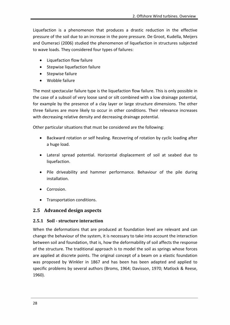
The following figure shows the scheme of these kinds of models in a laterally loaded
pile:
Figure 2.16: Soil idealization with springs
In structure engineering, springs are usually characterized by a constant stiffness,
which represents the relation between force and displacement: k=F/x. In the case of
soils, the relation between force and displacement is not always constant, therefore,
the stiffness of springs modelling soil depends on the displacement of the spring. The
relation between the soil lateral resistance force and the displacement is called the P‐y
curve. The following figure shows the P‐y curves of a laterally loaded pile:
2. Offshore Wind turbines. Overview
30
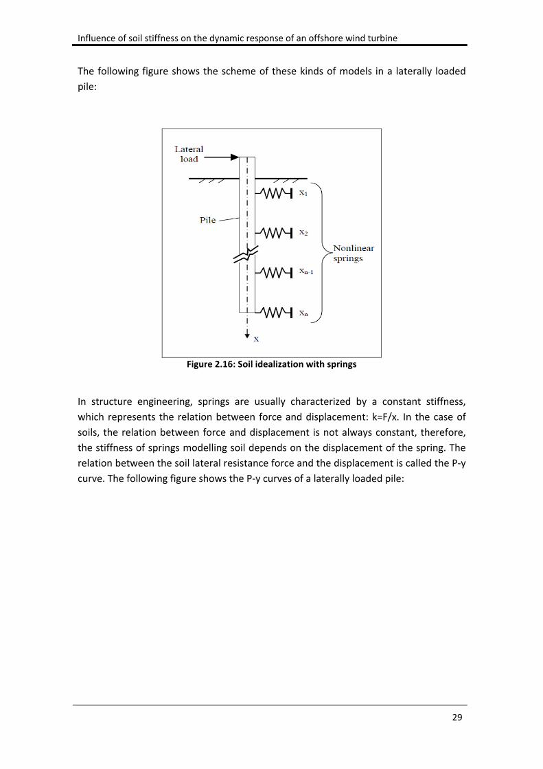
Figure 2.17: P‐y curves (DNV, 1992)
The P‐y curves are different at each depth, given that soil deformability changes with
depth and confinement. Therefore, each spring has associated a different curve P‐y. As
the depth increases, the stiffness of the curve is higher. The concept of P‐y curve is
associated with lateral displacement, but can be also extended to the others degrees
of freedom. Thereby, t‐z curve relates the tangential force at the pile shaft and the
vertical displacement; and Q‐z curve relates the vertical force at pile tip and the
vertical displacement.
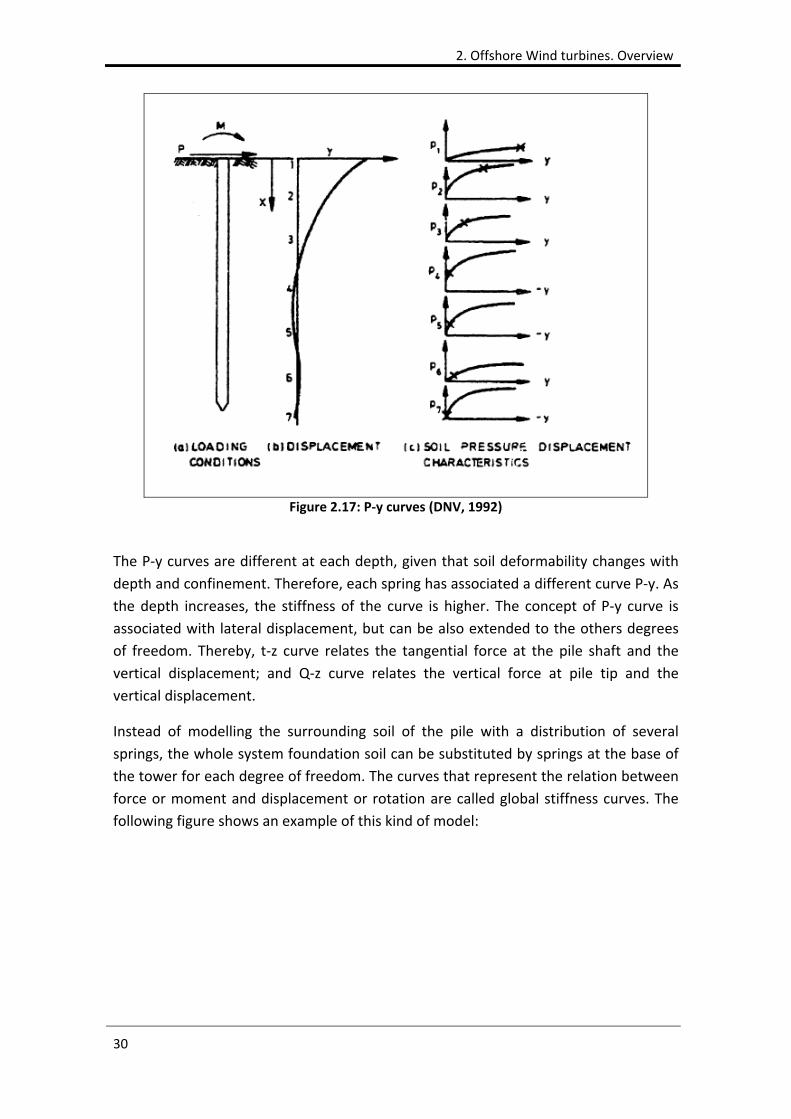
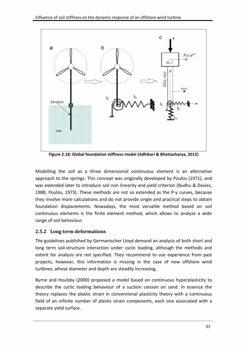
Instead of modelling the surrounding soil of the pile with a distribution of several
springs, the whole system foundation soil can be substituted by springs at the base of
the tower for each degree of freedom. The curves that represent the relation between
force or moment and displacement or rotation are called global stiffness curves. The
following figure shows an example of this kind of model:
Influence of soil stiffness on the dynamic response of an offshore wind turbine
31
Figure 2.18: Global foundation stiffness model (Adhikari & Bhattacharya, 2012)
Modelling the soil as a three dimensional continuous element is an alternative
approach to the springs. This concept was originally developed by Poulos (1971), and
was extended later to introduce soil non linearity and yield criterion (Budhu & Davies,
1988; Poulos, 1973). These methods are not so extended as the P‐y curves, because
they involve more calculations and do not provide single and practical steps to obtain
foundation displacements. Nowadays, the most versatile method based on soil
continuous elements is the finite element method, which allows to analyze a wide
range of soil behaviour.
2.5.2 Longtermdeformations
The guidelines published by Germanischer Lloyd demand an analysis of both short and
long term soil‐structure interaction under cyclic loading, although the methods and
extent for analysis are not specified. They recommend to use experience from past
projects, however, this information is missing in the case of new offshore wind
turbines, whose diameter and depth are steadily increasing.
Byrne and Houlsby (2000) proposed a model based on continuous hyperplasticity to
describe the cyclic loading behaviour of a suction caisson on sand. In essence the
theory replaces the plastic strain in conventional plasticity theory with a continuous
field of an infinite number of plastic strain components, each one associated with a
separate yield surface.
2. Offshore Wind turbines. Overview
32
The High‐Cycle Accumulation (HCA) model for sand (Niemunis, Wichtmann, &
Triantafyllidis, 2005) quantify the phenomenon of accumulation of stress and strain for
a large number of cycles of small amplitude. It is an empirical model based on
laboratory triaxial compression and extension tests. The main parameters of the model
are the following:
Accumulation rate of strain
Strain amplitude
Number of cycles
Average value of mean pressure during a cycle
Average stress ratio
Void ratio
Change of the polarization of the strain loop
The model follows an explicit calculation strategy, which can be summarized in the
following points:
Calculation of the initial stress field. The initial density can be obtained from
CPT / SPT values.
Implicit calculation of at least two first load cycles to obtain the spatial field of
strain amplitude. The authors use the hypoplasticity model with intergranular
strain for this purpose.
Recording of the strain path during the second cycle at each integration point.
Evaluate the tensorial strain amplitude from the recorded strain path. The
amplitude is assumed constant over all subsequent cycles, until it is
recalculated in a control cycle. The load cycles are grouped in packages of
constant amplitude and average value of bending moment and shear.
Find the accumulation rate of strain as the product of the parameters of the
model.
Find the stress increment caused by a package of N cycles.
The HCA model's authors studied the application of their model to offshore wind
foundations. Based on laboratory tests, they calibrated the model for a typical North
Sea fine sand and the parameters were used for FE calculations of an offshore
monopile foundation (Wichtmann, Niemunis, & Triantafyllidis, 2008). They concluded
that the application of the HCA model to offshore wind foundations has the following
particularities:
The HCA model is based on test with N<106 cycles, whereas an OWT is
subjected about N=108 cycles throughout its life.
It is necessary to consider changes in the polarization of the cycles due to
variations of the direction of wind and wave loading.
Influence of soil stiffness on the dynamic response of an offshore wind turbine
33
In case of scour protection it is necessary to determine the constants of the
HCA model for this material.
Galindo, Illueca, and Jimenez (2014) employed the HCA model to account for
accumulated deformations in a gas turbine submitted to a high number of cycles. The
cases of fine, poorly graded and medium density sand were studied. They observed
that transient situations at equipment's start‐up could be more restrictive than
stationary situations corresponding to normal operation. During these situations, a
wide range of frequencies is traversed, including frequencies that could be similar to
the natural frequencies of the ground.
LeBlanc, Houlsby and Byrne (2009) have studied the response of a monopile
foundation in sand to long term cyclic lateral loading. They conducted laboratory tests
where a small scale pile was subjected to between 8000 and 60000 cycles of combined
moment and horizontal loading. The authors concluded that accumulated rotation is
largely affected by the cyclic characteristics of the load. The typical tolerances for
accumulated rotation are breached if the foundation is designed considering the ULS
load, which suggests that accumulated rotation is the primary design driver. They also
concluded that cyclic loading increases the pile stiffness, independently of relative
density, which contrasts with the current methodology of degrading static p‐y curves.
Cuellar (2011) studied both long and short term effects of cyclic loading in an offshore
monopile foundation. In the short term, the foundation can be affected by transient
episodes of softening as a consequence of pore pressure accumulation, whereas in the
long term, the hardening and soil densification can affect the serviceability of the
structure. The author used the Finite Element Method to analyze the short term
effects and studied the long term effects by means of model tests in a reduced scale.
His main conclusions were the following:
In the short term, cyclic lateral displacements caused by extreme loads
produce a net accumulation of pore pressure in the soil due to a progressive
reduction of pore volume and the inability of the soil to dissipate the
overpressure between consecutive cycles.
The accumulation of pore pressure in the short term produces a decrease of
effective stress in the soil and can lead to considerable plastic deformations.
An increase of pile diameter can have a beneficial effect on the accumulation
rate of pore pressure due to the lower levels of pile displacement and soil
compression.
In the long term, a progressive reduction of bending moments was observed
due to an increasing rigidization of the upper layers of soil.
The general trend in the long term can be described as an attenuating
incremental deformation.
2. Offshore Wind turbines. Overview
34
The densification of soil around the pile causes a general subsidence,
independently of scour phenomena, and affects the dynamic behaviour of the
foundation. The increase in stiffness of the soil and the reduction in
embedment change the natural frequency of the structure.
Experimental model tests on shallow foundations on dense sand have shown that
cyclic loads following a single huge load lead to a backward rotation of the foundation
(Wienbroer, Zachert, & Triantafyllidis, 2011). The authors explain this rotation by
different compaction rates due to uneven void ratios on the leeward and the
windward side. They introduce the Backward Rotation Index, BRI, to quantify the
rotation. 1000 cycles are sufficient to revert about 70% of the rotation due to the
maximum force.
2.5.3 Probabilisticapproach
Uncertainties in values of model parameters are especially relevant in geotechnics.
Unlike concrete or steel, soil is not a manufactured product submitted to a quality‐
controlled process, therefore, it is difficult to guarantee a certain value of its
properties. A proper characterization of soil must take into account the grade of
uncertainty of its parameters. This characterization of uncertainties in the input
parameters of a given model allows designers to evaluate their impact on the results.
The aim of a reliability analysis is to quantify the probability of failure of a given design,
with the concept of "probability of failure" referring to situations in which the design is
not fulfilling its purpose, considering it in a general sense so that it can be applied to
any limit state.
There are several methods to assess the reliability of a design, each one with a
different degree of complexity. They can be divided into the following four levels
(Mínguez, 2003):
Level 1: These methods do not calculate probability of failure. The grade of
uncertainty is measured by partial safety factors, which are selected for each
variable, such as load or strength. It is the traditional way and the most used
in several codes.
Level 2: The probability of failure, Pf, is calculated from the integral of the
joint probability density function of all variables of the problem. The main
disadvantage of these methods is that the integral is difficult to calculate
because of the complexity of both the density function and the limit state
surface that defines the integration domain. It is therefore necessary to
approximate the density function, which at this level is done by taking the
two first moments of the joint probability density function.
Influence of soil stiffness on the dynamic response of an offshore wind turbine
35
Level 3: The probability of failure is calculated by means of the global joint
probability function. These methods calculate the better approximations to
the exact probability of failure, and require specific integration techniques
and methodologies. The most common methods in this level are FORM,
SORM and Montecarlo.
A fourth level is mentioned in some texts in which an economic factor is taken into
account. The aim of these methods is to minimize the cost or to maximize the profits.
They involve principles of engineering economic analysis under uncertainty and the
problem variables are usually cost and benefits of construction, maintenance, repair,
consequences of failure, interest on capital and so on.
Methods in level 2 work with independent variables which follow a normal
distribution. In the case of dependent variables, they have to be transformed. A linear
approximation (First Order) of the limit state surface is used to estimate the probability
of failure. The probability density function is characterized by its two first moments
(Second Moment). These methods take their name from the two mentioned
assumptions: FOSM (First Order Second Moment). The main limitation of these
methods is that they are only exact with normal distributions and linear limit state
surfaces.
The First Order Reliability Methods (FORM) also uses a linear approximation of the
limit state surface, but it works with the exact density functions of the variables. The
Second Order Reliability Methods approximate the limit state surface by means of a
second order polynomial surface. They are very precise methods and much more
efficient than Montecarlo simulations.
The Montecarlo method is based on computing a large number of simulations for
different realizations of the stochastic variables. This values are taken randomly, so the
number of simulations has to be large enough to cover a representative range of
events (Metropolis & Ulam, 1949).
2.6 Solutionsandimprovements
In this section, some solutions that have been either proposed or adopted previously
to mitigate the problems that affect these structures are described. Given that this is a
complex and very changing field, they will be only listed and described briefly. It is
outside the scope of this study to explain the details of each solution:
Tuned liquid column damper (TLCD). It is a U‐shaped tube which is partially
filled with liquid and attached to the structure. The liquid oscillations when the
tower is excited help to restore the equilibrium. They can increase the fatigue
life of the structure (Colwell & Basu, 2009).
2. Offshore Wind turbines. Overview
36
Roughness in skirted foundations. An increase in roughness in the wall of this
foundation generates more friction between the steel and soil and improves
the uplift resistance.
Reduction of gap. A mitigation of gap initiation and propagation in skirted
foundations would increase the uplift strength.
Electrokinetic strengthening of soil. Laboratory experiments carried out on
clays surrounding skirted foundations have shown an increase in the undrained
shear strength of soil, which enhances the uplift resistance (Micic, Shang, & Lo,
2002).
Scour protection. Several studies have been carried out in order to design
protection measures against scour. The main solutions are blankets or a layer
of ballast around the foundation (De Vos, De Rouck, Troch, & Frigaard, 2011).
Reduction of cavity depth. The flow failure in spudcan foundations during the
penetration stage can be avoided by limiting the cavity depth (Hossain et al.,
2005).
In the case of grouted connections, there are three main measures that can be
taken to avoid fatigue failure:
Shear keys. In the form of welded‐on profiles, they increase the axial bearing
capacity. They contribute to transfer the bending moment by vertical
circumferential forces. They reduce the interface opening at the top and the
bottom.
Conical connections. They transfer the axial load without relying on the bond
capacity.
Additional supports.
2.7 Codes
The main codes, recommendations or guidelines that are used in the design and
construction of an offshore wind turbine are listed as follows. Some of them are
specific of wind turbines and others were developed for general offshore structures,
mainly for the petroleum industry. The main organizations that have developed these
codes are the International Organization for Standardization (ISO), Det Norske Veritas
(DNV) and Germanischer Lloyd (GL). Norsok standards (N) are developed by the
Norwegian petroleum industry.
ISO 19900 (2013). Petroleum and natural gas industries. General requirements for
offshore structures.
Influence of soil stiffness on the dynamic response of an offshore wind turbine
37
ISO 19902 (2007). Petroleum and natural gas industries. Fixed steel offshore
structures.
ISO 19903 (2006). Petroleum and natural gas industries. Fixed concrete offshore
structures.
DNV‐OS‐J101 (2014). Design of offshore wind turbine structures.
DNV‐RP‐C203 (2011). Fatigue design of offshore steel structures.
DNV‐RP‐C204 (2010). Design against accidental loads.
DNV‐RP‐C205 (2010). Environmental conditions and environmental loads.
DNV‐CN‐30.4 (1992). Foundations.
GL‐IV‐2 (2012). Guideline for the Certification of Offshore Wind Turbines.
GL‐IV‐6‐4 (2007). Offshore Technology. Structural design.
GL‐IV‐6‐7 (2005). Offshore installations. Guideline for the construction of fixed
offshore installations in ice infested waters.
N‐003 (2007). Actions and actions effects.
N‐004 (2013). Design of steel structures.
API‐RP‐2A‐LRFD (1993). Recommended practice for planning, designing and
constructing fixed offshore platforms. Load and resistance factor design.
API‐RP‐2A‐WSD (2014). Recommended practice for planning, designing and
constructing fixed offshore platforms. Working stress design

Influence of soil stiffness on the dynamic response of an offshore wind turbine
39
3 Caseofstudy
3.1 Introduction
The behaviour of an offshore wind turbine under both monotonic and cyclic loading
has been studied by means of a finite element model implemented in the software
Abaqus. The tower is founded on a steel monopile in sand. In order to study the
influence of the soil properties on the response of the structure, several cases have
been analyzed with different soil stiffness.
3.2 Structureandloadproperties
The geometry of the structure is typical of an offshore wind turbine installed in water
depths around 30m. Its main properties are as follows:
Length of the tower over the seabed: 100m
Foundation depth: 30m
External diameter of tower and monopile: 6m
Thickness: 0.075m
Steel density: 8450 kg/m3
Friction coefficient steel‐sand: 0.3
Young modulus of steel: 205 GPa
Poisson coefficient of steel: 0.3
Mass of nacelle, hub and rotor blades: 336 tn
The load acting on the structure is the wind force, which is applied as a horizontal
concentrated force in the rotor. Two different loads have been considered:
Monotonic load:
o Magnitude: 700 kN
Sinusoidal load:
o Mean: 600 kN
o Amplitude: 100 kN
o Angular velocity: 1.65 rad/s
3. Case of study
40
The load has been chosen from a study of a similar tower so that its magnitude is an
intermediate value between the normal operative case and the extreme sea state
(Garcés García, 2012). The maximum value of the cyclic force is equal to the static
force, so the structure is under the same load magnitude in both cases.
The angular velocity of the cyclic load has been chosen to be within the range of
natural frequencies obtained in the dynamical analysis for different soils. Therefore,
the dynamic amplification of the response of the structure can be studied for different
ratios of natural frequency to load frequency. The load frequency considered is high
for the most usual wind spectrums but is close to 3P, therefore, it is representative of
the shadowing effect produced by the blades.
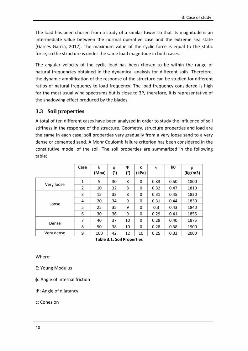
3.3 Soilproperties
A total of ten different cases have been analyzed in order to study the influence of soil
stiffness in the response of the structure. Geometry, structure properties and load are
the same in each case; soil properties vary gradually from a very loose sand to a very
dense or cemented sand. A Mohr Coulomb failure criterion has been considered in the
constitutive model of the soil. The soil properties are summarized in the following
table:
Case E (Mpa)
(°)
(°)
c (kPa)
k0 (Kg/m3)
Very loose 1 5 30 8 0 0.33 0.50 1800
2 10 32 8 0 0.32 0.47 1810
Loose
3 15 33 8 0 0.31 0.45 1820
4 20 34 9 0 0.31 0.44 1830
5 25 35 9 0 0.3 0.43 1840
6 30 36 9 0 0.29 0.41 1855
Dense 7 40 37 10 0 0.28 0.40 1875
8 50 38 10 0 0.28 0.38 1900 Very dense 9 100 42 12 10 0.25 0.33 2000
Table 3.1: Soil Properties
Where:
E: Young Modulus
: Angle of internal friction
: Angle of dilatancy
c: Cohesion
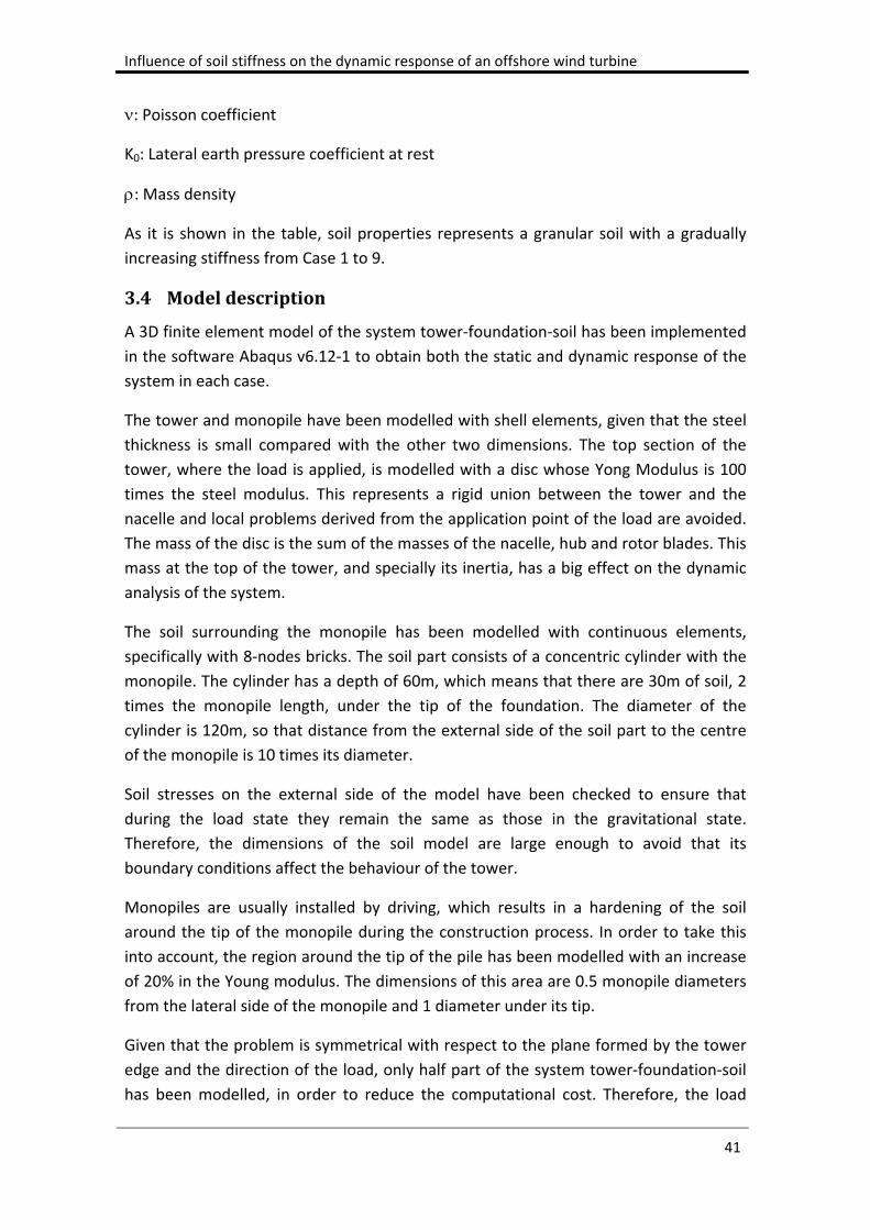
Influence of soil stiffness on the dynamic response of an offshore wind turbine
41
: Poisson coefficient
K0: Lateral earth pressure coefficient at rest
: Mass density
As it is shown in the table, soil properties represents a granular soil with a gradually
increasing stiffness from Case 1 to 9.
3.4 Modeldescription
A 3D finite element model of the system tower‐foundation‐soil has been implemented
in the software Abaqus v6.12‐1 to obtain both the static and dynamic response of the
system in each case.
The tower and monopile have been modelled with shell elements, given that the steel
thickness is small compared with the other two dimensions. The top section of the
tower, where the load is applied, is modelled with a disc whose Yong Modulus is 100
times the steel modulus. This represents a rigid union between the tower and the
nacelle and local problems derived from the application point of the load are avoided.
The mass of the disc is the sum of the masses of the nacelle, hub and rotor blades. This
mass at the top of the tower, and specially its inertia, has a big effect on the dynamic
analysis of the system.
The soil surrounding the monopile has been modelled with continuous elements,
specifically with 8‐nodes bricks. The soil part consists of a concentric cylinder with the
monopile. The cylinder has a depth of 60m, which means that there are 30m of soil, 2
times the monopile length, under the tip of the foundation. The diameter of the
cylinder is 120m, so that distance from the external side of the soil part to the centre
of the monopile is 10 times its diameter.
Soil stresses on the external side of the model have been checked to ensure that
during the load state they remain the same as those in the gravitational state.
Therefore, the dimensions of the soil model are large enough to avoid that its
boundary conditions affect the behaviour of the tower.
Monopiles are usually installed by driving, which results in a hardening of the soil
around the tip of the monopile during the construction process. In order to take this
into account, the region around the tip of the pile has been modelled with an increase
of 20% in the Young modulus. The dimensions of this area are 0.5 monopile diameters
from the lateral side of the monopile and 1 diameter under its tip.
Given that the problem is symmetrical with respect to the plane formed by the tower
edge and the direction of the load, only half part of the system tower‐foundation‐soil
has been modelled, in order to reduce the computational cost. Therefore, the load
3. Case of study
42
applied to the head of the model has to be half the actual load. The displacements in
perpendicular direction to the plane of symmetry have to be zero, which is introduced
as a boundary condition. The rest of boundary conditions are applied to the external
sides of the soil part: zero vertical displacement at the base of the cylinder and zero
horizontal displacement, along any of the two edges, on the external vertical side of
the cylinder.
In order to simulate the contact between the soil and the monopile, master and slave
surfaces have been implemented. The external side of the monopile is the master
surface and the adjacent soil is the slave. The normal behaviour is defined as a hard
contact, which means that the master surface cannot cross the slave, and separation
of both surfaces is allowed after contact without any tensile strength. The tangential
behaviour is defined by a friction coefficient between both surfaces. A tangential force
is generated when there is relative displacement between both surfaces, its magnitude
being the normal force multiplied by the friction coefficient.
The soil column inside the monopile has not been modelled because the state of this
soil after the construction process and its contribution to friction resistance is not
clear. However, its weight has been taken into account as a pressure under the
monopile tip.
The following figure shows a global view of the mesh, main dimensions, loads and
boundary conditions, Ui being the displacement along the i‐axis:
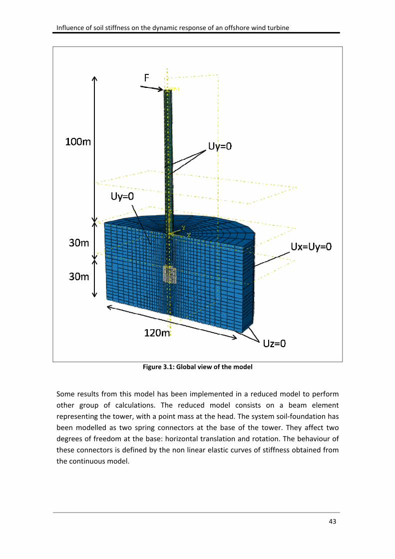
Influence of soil stiffness on the dynamic response of an offshore wind turbine
43
Figure 3.1: Global view of the model
Some results from this model has been implemented in a reduced model to perform
other group of calculations. The reduced model consists on a beam element
representing the tower, with a point mass at the head. The system soil‐foundation has
been modelled as two spring connectors at the base of the tower. They affect two
degrees of freedom at the base: horizontal translation and rotation. The behaviour of
these connectors is defined by the non linear elastic curves of stiffness obtained from
the continuous model.
3. Case of study
44
3.5 Analysesperformed
Two main groups of analyses have been performed in this study. The first one has been
applied to the 9 cases of different soils detailed in the paragraph "Soil properties". Its
aim is to obtain the displacement at the head of the tower, the natural frequency of
the system and the range of cyclic stresses in the steel.
The second group of analyses has been applied to the case nº 4 and its aim is to obtain
the relationship between displacements and forces in the foundation. These results
are implement in a simplified model in which the soil is substituted by its reaction
forces and moments on the tower, which are obtained from the curves force‐
displacement (P‐y) and moment‐angle (M‐).
The first group of analyses, which are applied to the 9 cases, is formed by the following
states:
Static load
Free oscillation
Forced oscillation
The first state consists of a static analysis in which a constant horizontal load of 700 kN
is applied to the head of the tower. This state is divided into two consecutive load
steps: gravity and static load. The main result obtained is the horizontal displacement
at the head of the tower.
The free oscillation state consists of the application of a static load of 700 kN to the
head of the tower and then, from this equilibrium state, the load is removed and a
dynamic implicit analysis is performed in which the tower is oscillating freely during 20
seconds. There are three consecutive load steps in this state: gravity, static load and
free oscillation. The objective of this analysis is to obtain the oscillation frequency of
the tower, which is measured from the displacement at the head of the tower over
time.
The state of free oscillation is a non standard way to obtain the natural frequency of
the system. The usual way to calculate this in a structure is to perform a modal
analysis, however, in this case there are some particularities which difficult the
application of this method. The main one is the high number of degrees of freedom
that the soil part introduces in the model. The soil nodes result in a great amount of
modes of vibration that are not relevant or hardly contribute to the response of the
structure. For example, a vertical oscillation of the soil nodes located in the external
area of the model do not mobilize any mass of the tower. Another problem is that a
modal analysis implies a linear response and a symmetrical stiffness matrix. The
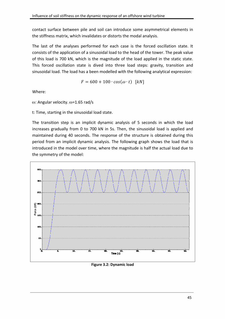
Influence of soil stiffness on the dynamic response of an offshore wind turbine
45
contact surface between pile and soil can introduce some asymmetrical elements in
the stiffness matrix, which invalidates or distorts the modal analysis.
The last of the analyses performed for each case is the forced oscillation state. It
consists of the application of a sinusoidal load to the head of the tower. The peak value
of this load is 700 kN, which is the magnitude of the load applied in the static state.
This forced oscillation state is dived into three load steps: gravity, transition and
sinusoidal load. The load has a been modelled with the following analytical expression:
600 100 ∙ ∙
Where:
: Angular velocity. =1.65 rad/s
t: Time, starting in the sinusoidal load state.
The transition step is an implicit dynamic analysis of 5 seconds in which the load
increases gradually from 0 to 700 kN in 5s. Then, the sinusoidal load is applied and
maintained during 40 seconds. The response of the structure is obtained during this
period from an implicit dynamic analysis. The following graph shows the load that is
introduced in the model over time, where the magnitude is half the actual load due to
the symmetry of the model:
Figure 3.2: Dynamic load
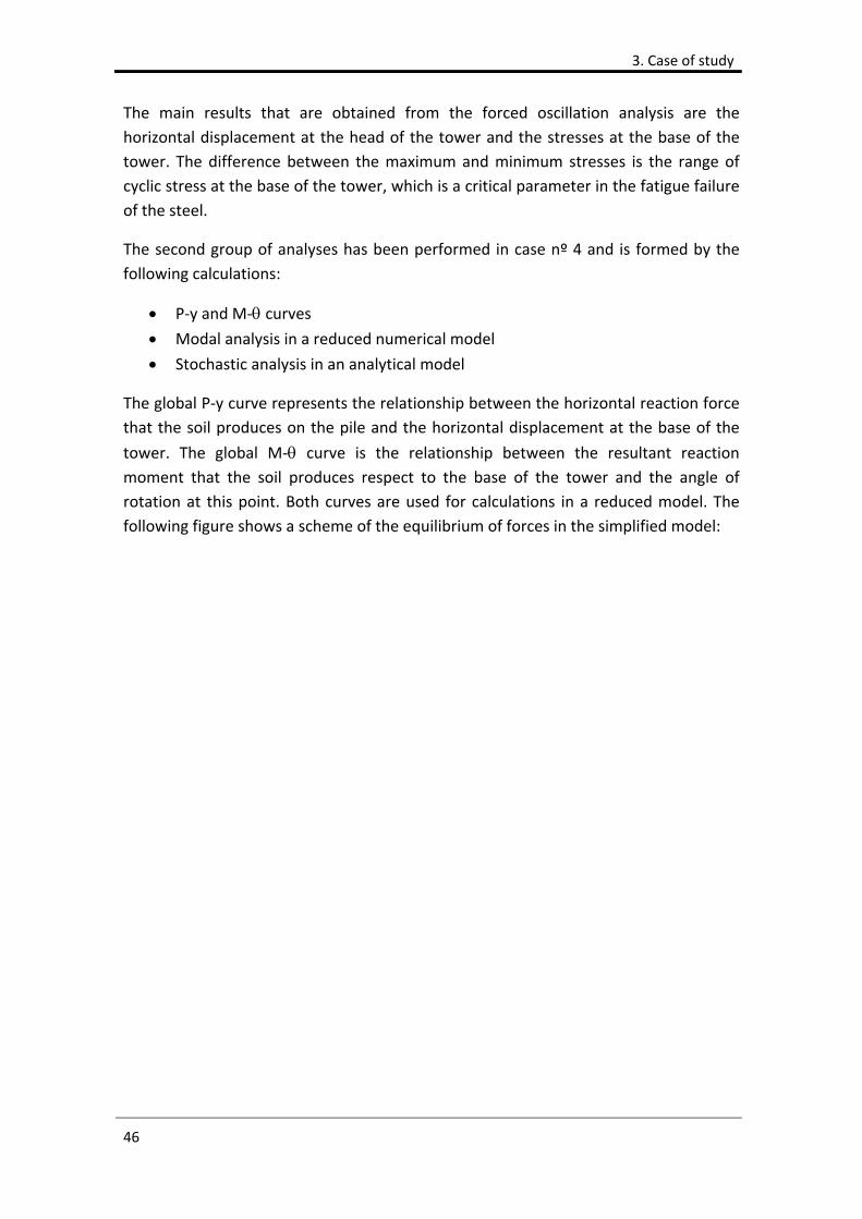
3. Case of study
46
The main results that are obtained from the forced oscillation analysis are the
horizontal displacement at the head of the tower and the stresses at the base of the
tower. The difference between the maximum and minimum stresses is the range of
cyclic stress at the base of the tower, which is a critical parameter in the fatigue failure
of the steel.
The second group of analyses has been performed in case nº 4 and is formed by the
following calculations:
P‐y and M‐ curves Modal analysis in a reduced numerical model
Stochastic analysis in an analytical model
The global P‐y curve represents the relationship between the horizontal reaction force
that the soil produces on the pile and the horizontal displacement at the base of the
tower. The global M‐ curve is the relationship between the resultant reaction moment that the soil produces respect to the base of the tower and the angle of
rotation at this point. Both curves are used for calculations in a reduced model. The
following figure shows a scheme of the equilibrium of forces in the simplified model:
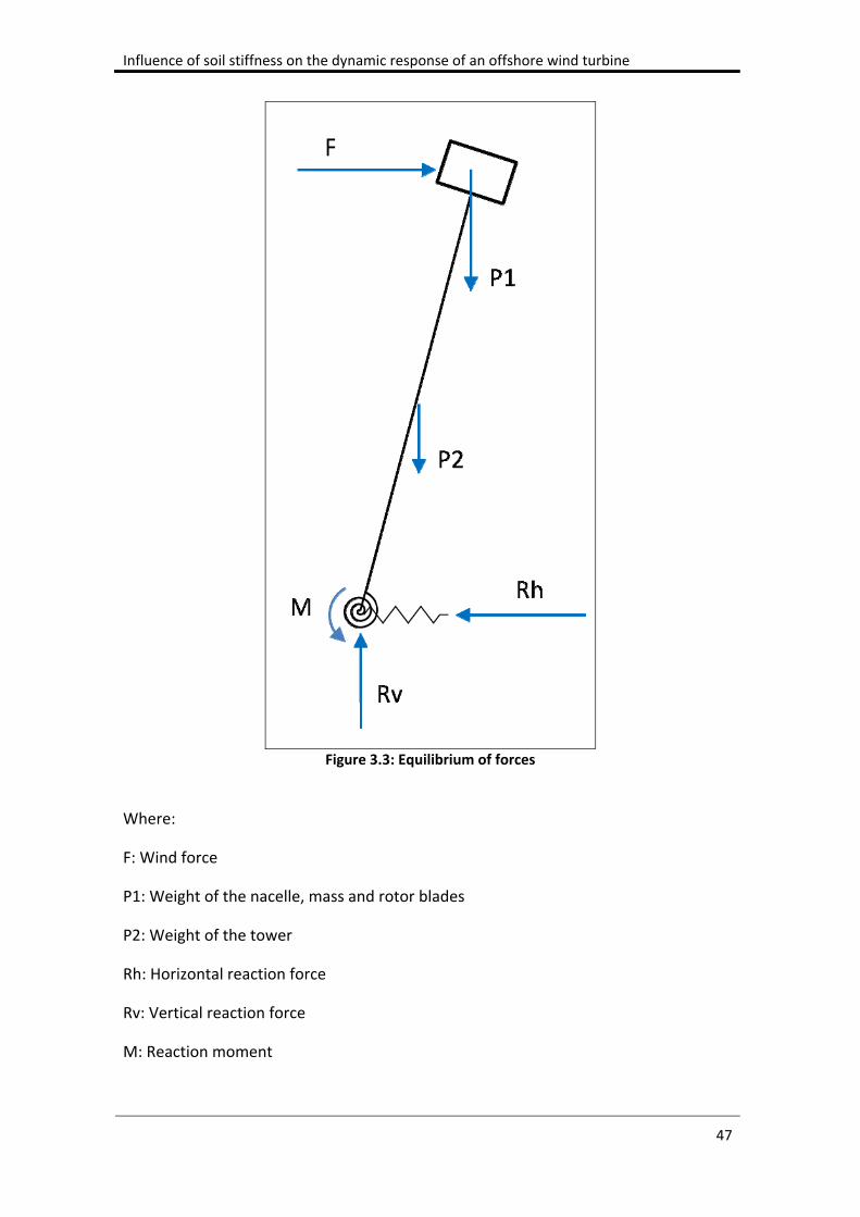
Influence of soil stiffness on the dynamic response of an offshore wind turbine
47
Figure 3.3: Equilibrium of forces
Where:
F: Wind force
P1: Weight of the nacelle, mass and rotor blades
P2: Weight of the tower
Rh: Horizontal reaction force
Rv: Vertical reaction force
M: Reaction moment
3. Case of study
48
The soil is substituted by two degrees of freedom at the base of the tower: horizontal
displacement and rotation respect to an edge which is perpendicular to the scheme. In
order to simplify the analysis, the vertical displacement at the base of the tower is
considered to be zero. The two degrees of freedom of the foundation are contained in
the plane formed by the tower and the wind force F, therefore, it is a 2D model. Both
degrees of freedom are considered to be uncoupled and they are characterized by two
elastic springs. The horizontal reaction force Rh and the horizontal displacement at the
base of the tower lead to the P‐y curve. The reaction moment M and the angle of
rotation at the base of the tower lead to the M‐ curve.
Each point of the foundation behaviour curves is obtained from an equilibrium state
for a given value of the wind force, F. A total of ten points have been calculated to
define each curve, increasing gradually the value of F from 0 to 4000 kN and
performing a static analysis in each load increment. The reaction forces can be
obtained from the equilibrium equations:
1 ∗ 1 2 ∗ 2 ∗
Where:
d1: Horizontal displacement at the head of the tower
d2: Horizontal displacement at the middle point of the tower
Ht: Height of the tower
In addition to the global P‐y and M‐ curves, which refer to the base of the tower, the P‐y curve at a given depth has also been obtained, that is, the lateral reaction of the
soil per unit length at a given depth versus the lateral deflection. These kind of curves
are used in Winkler models, where the soil is substituted by several springs.
In the model analyzed, the P‐y curve for one of these springs have been obtained from
the reactions on the contact surface at a given depth. This curve can be compared with
that given in the DNV code, which is obtained from the following expression, valid for a
laterally loaded pile in a cohesionless soil:
∙ ∙∙∙
∙
Where:
A: Factor to account for cyclic or static loading. For static loading:
Influence of soil stiffness on the dynamic response of an offshore wind turbine
49
3 0.8 0.9
H: Length (m)
D: Pile diameter (m)
Pu: Lateral resistance of soil per unit length (kN/m)
k: Initial modulus of subgrade reaction (MN/m3). Obtained as a function of
x: Depth (m)
y: Lateral deflection (mm)
The global P‐y and M‐ curves are implemented in a simplified model with the scheme
given in figure 3.3. The soil part has been changed for springs and, therefore, a
considerable reduction in the degrees of freedom in the foundation is produced. This
reduction allows to perform a modal analysis to obtain the natural frequency of the
reduced model. This natural frequency has been calculated and compared with that
obtained by means of the free oscillation of the whole model. The reduced model has
also been used to obtain the dynamic response under a cyclic load. In this way, the
goodness of the soil behaviour curves obtained from a static analysis can be assessed
for their use in a dynamic analysis.
Finally, a stochastic analysis of the natural frequency is carried out by following the
analytical methodology proposed by Adhikari & Bhattacharya (2012). In this model, the
foundation behaviour is represented by two degrees of freedom at the base of the
tower: horizontal translation and rotation. The global P‐y and M‐ curves are used to obtain the mean values of the translation stiffness, Kt, and rotation stiffness, Kr. These
parameters are considered as independent stochastic variables characterized by a
lognormal distribution.
The natural frequency is obtained from the free vibration problem by considering no
force on the system. The details of the analysis process to reach the solution are given
by the authors. The problem is reduced to solve the following equation:
| | 0
Where R is the following 4x4 matrix:
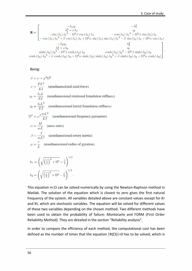
3. Case of study
50
Being:
This equation in can be solved numerically by using the Newton‐Raphson method in
Matlab. The solution of the equation which is closest to zero gives the first natural
frequency of the system. All variables detailed above are constant values except for Kr
and Kt, which are stochastic variables. The equation will be solved for different values
of these two variables depending on the chosen method. Two different methods have
been used to obtain the probability of failure: Montecarlo and FORM (First Order
Reliability Method). They are detailed in the section "Reliability analysis".
In order to compare the efficiency of each method, the computational cost has been
defined as the number of times that the equation |R()|=0 has to be solved, which is

Influence of soil stiffness on the dynamic response of an offshore wind turbine
51
where the most number of operations are computed and, therefore, what consume
most part of the time.

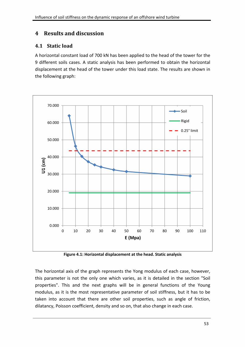
Influence of soil stiffness on the dynamic response of an offshore wind turbine
53
4 Resultsanddiscussion
4.1 Staticload
A horizontal constant load of 700 kN has been applied to the head of the tower for the
9 different soils cases. A static analysis has been performed to obtain the horizontal
displacement at the head of the tower under this load state. The results are shown in
the following graph:
Figure 4.1: Horizontal displacement at the head. Static analysis
The horizontal axis of the graph represents the Yong modulus of each case, however,
this parameter is not the only one which varies, as it is detailed in the section "Soil
properties". This and the next graphs will be in general functions of the Young
modulus, as it is the most representative parameter of soil stiffness, but it has to be
taken into account that there are other soil properties, such as angle of friction,
dilatancy, Poisson coefficient, density and so on, that also change in each case.
0.000
10.000
20.000
30.000
40.000
50.000
60.000
70.000
0 10 20 30 40 50 60 70 80 90 100 110
U1 (cm
)
E (Mpa)
Soil
Rigid
0.25° limit
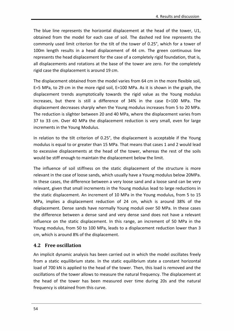
4. Results and discussion
54
The blue line represents the horizontal displacement at the head of the tower, U1,
obtained from the model for each case of soil. The dashed red line represents the
commonly used limit criterion for the tilt of the tower of 0.25°, which for a tower of
100m length results in a head displacement of 44 cm. The green continuous line
represents the head displacement for the case of a completely rigid foundation, that is,
all displacements and rotations at the base of the tower are zero. For the completely
rigid case the displacement is around 19 cm.
The displacement obtained from the model varies from 64 cm in the more flexible soil,
E=5 MPa, to 29 cm in the more rigid soil, E=100 MPa. As it is shown in the graph, the
displacement trends asymptotically towards the rigid value as the Young modulus
increases, but there is still a difference of 34% in the case E=100 MPa. The
displacement decreases sharply when the Young modulus increases from 5 to 20 MPa.
The reduction is slighter between 20 and 40 MPa, where the displacement varies from
37 to 33 cm. Over 40 MPa the displacement reduction is very small, even for large
increments in the Young Modulus.
In relation to the tilt criterion of 0.25°, the displacement is acceptable if the Young
modulus is equal to or greater than 15 MPa. That means that cases 1 and 2 would lead
to excessive displacements at the head of the tower, whereas the rest of the soils
would be stiff enough to maintain the displacement below the limit.
The influence of soil stiffness on the static displacement of the structure is more
relevant in the case of loose sands, which usually have a Young modulus below 20MPa.
In these cases, the difference between a very loose sand and a loose sand can be very
relevant, given that small increments in the Young modulus lead to large reductions in
the static displacement. An increment of 10 MPa in the Young modulus, from 5 to 15
MPa, implies a displacement reduction of 24 cm, which is around 38% of the
displacement. Dense sands have normally Young moduli over 50 MPa. In these cases
the difference between a dense sand and very dense sand does not have a relevant
influence on the static displacement. In this range, an increment of 50 MPa in the
Young modulus, from 50 to 100 MPa, leads to a displacement reduction lower than 3
cm, which is around 8% of the displacement.
4.2 Freeoscillation
An implicit dynamic analysis has been carried out in which the model oscillates freely
from a static equilibrium state. In the static equilibrium state a constant horizontal
load of 700 kN is applied to the head of the tower. Then, this load is removed and the
oscillations of the tower allows to measure the natural frequency. The displacement at
the head of the tower has been measured over time during 20s and the natural
frequency is obtained from this curve.
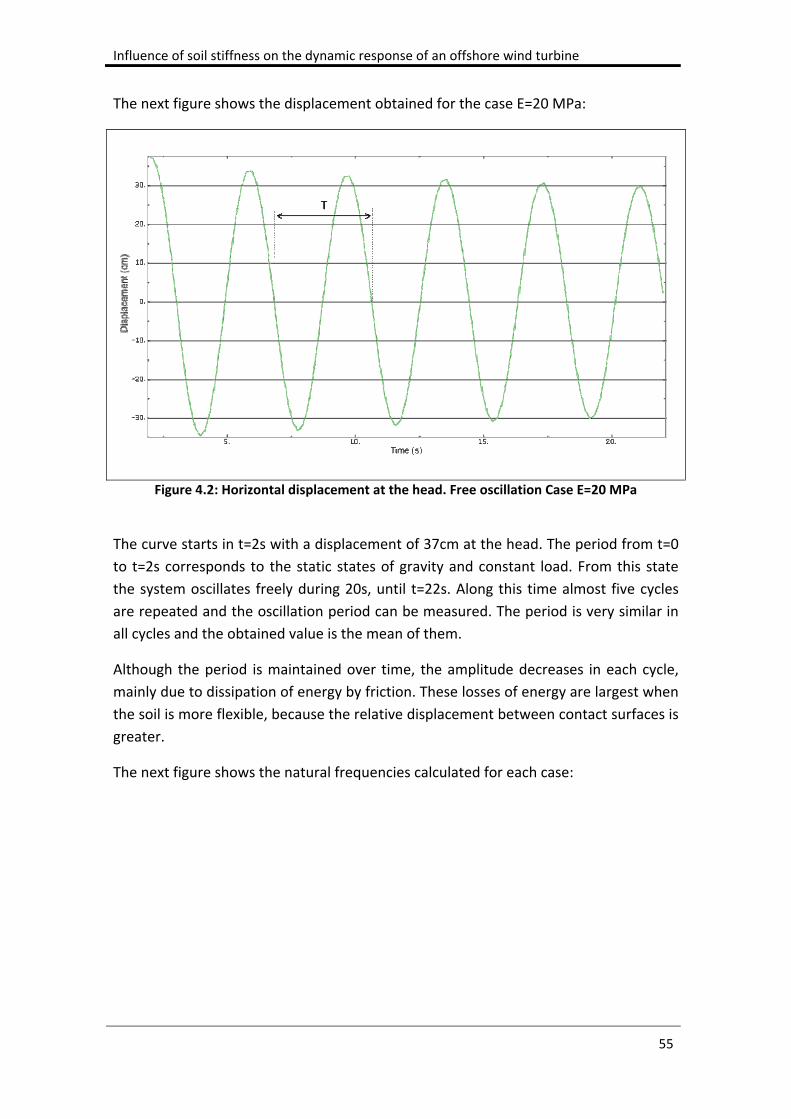
Influence of soil stiffness on the dynamic response of an offshore wind turbine
55
The next figure shows the displacement obtained for the case E=20 MPa:
Figure 4.2: Horizontal displacement at the head. Free oscillation Case E=20 MPa
The curve starts in t=2s with a displacement of 37cm at the head. The period from t=0
to t=2s corresponds to the static states of gravity and constant load. From this state
the system oscillates freely during 20s, until t=22s. Along this time almost five cycles
are repeated and the oscillation period can be measured. The period is very similar in
all cycles and the obtained value is the mean of them.
Although the period is maintained over time, the amplitude decreases in each cycle,
mainly due to dissipation of energy by friction. These losses of energy are largest when
the soil is more flexible, because the relative displacement between contact surfaces is
greater.
The next figure shows the natural frequencies calculated for each case:
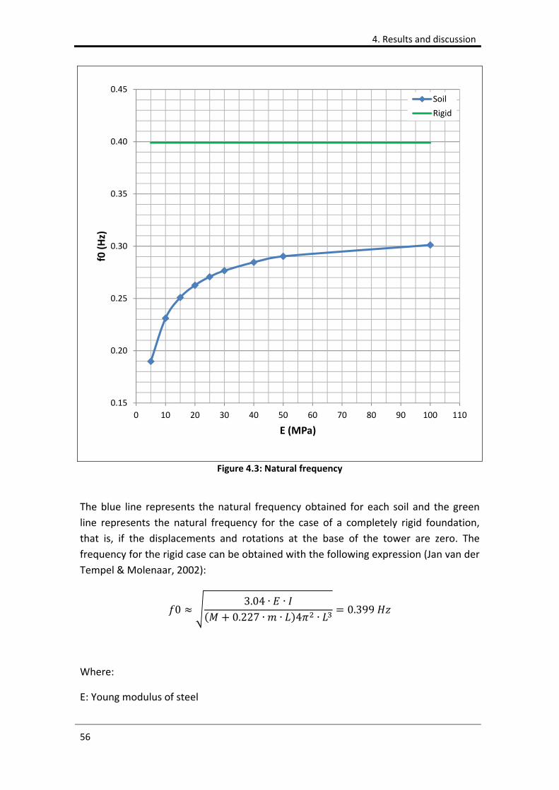
4. Results and discussion
56
Figure 4.3: Natural frequency
The blue line represents the natural frequency obtained for each soil and the green
line represents the natural frequency for the case of a completely rigid foundation,
that is, if the displacements and rotations at the base of the tower are zero. The
frequency for the rigid case can be obtained with the following expression (Jan van der
Tempel & Molenaar, 2002):
03.04 ∙ ∙
0.227 ∙ ∙ 4 ∙0.399
Where:
E: Young modulus of steel
0.15
0.20
0.25
0.30
0.35
0.40
0.45
0 10 20 30 40 50 60 70 80 90 100 110
f0 (Hz)
E (MPa)
Soil
Rigid
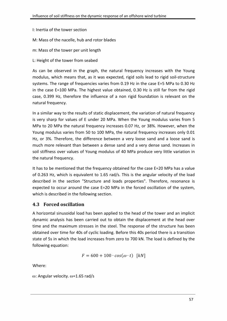
Influence of soil stiffness on the dynamic response of an offshore wind turbine
57
I: Inertia of the tower section
M: Mass of the nacelle, hub and rotor blades
m: Mass of the tower per unit length
L: Height of the tower from seabed
As can be observed in the graph, the natural frequency increases with the Young
modulus, which means that, as it was expected, rigid soils lead to rigid soil‐structure
systems. The range of frequencies varies from 0.19 Hz in the case E=5 MPa to 0.30 Hz
in the case E=100 MPa. The highest value obtained, 0.30 Hz is still far from the rigid
case, 0.399 Hz, therefore the influence of a non rigid foundation is relevant on the
natural frequency.
In a similar way to the results of static displacement, the variation of natural frequency
is very sharp for values of E under 20 MPa. When the Young modulus varies from 5
MPa to 20 MPa the natural frequency increases 0.07 Hz, or 38%. However, when the
Young modulus varies from 50 to 100 MPa, the natural frequency increases only 0.01
Hz, or 3%. Therefore, the difference between a very loose sand and a loose sand is
much more relevant than between a dense sand and a very dense sand. Increases in
soil stiffness over values of Young modulus of 40 MPa produce very little variation in
the natural frequency.
It has to be mentioned that the frequency obtained for the case E=20 MPa has a value
of 0.263 Hz, which is equivalent to 1.65 rad/s. This is the angular velocity of the load
described in the section "Structure and loads properties". Therefore, resonance is
expected to occur around the case E=20 MPa in the forced oscillation of the system,
which is described in the following section.
4.3 Forcedoscillation
A horizontal sinusoidal load has been applied to the head of the tower and an implicit
dynamic analysis has been carried out to obtain the displacement at the head over
time and the maximum stresses in the steel. The response of the structure has been
obtained over time for 40s of cyclic loading. Before this 40s period there is a transition
state of 5s in which the load increases from zero to 700 kN. The load is defined by the
following equation:
600 100 ∙ ∙
Where:
: Angular velocity. =1.65 rad/s
4. Results and discussion
58
t: Time, starting in the sinusoidal load state.
The next three graphs show the horizontal displacement of the head of the tower for
the cases E=10, 20 and 40 MPa. As it was showed in the section "Free oscillation", in
the case E=10 MPa the natural frequency is lower than the load frequency, both
frequencies are equal in the case E=20 MPa, and the natural frequency is higher than
the load frequency in the case E=40 MPa.
Figure 4.4: Horizontal displacement at the head. Forced oscillation Case E=10 MPa (f0<)
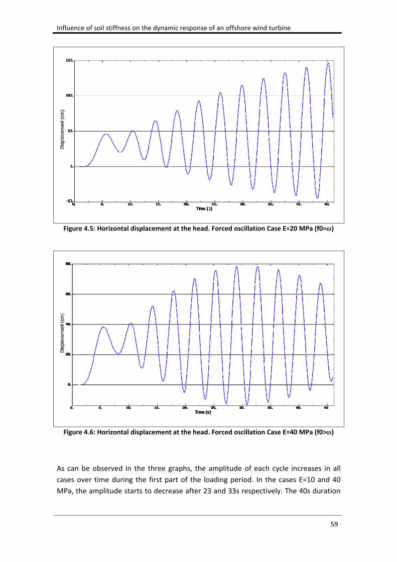
Influence of soil stiffness on the dynamic response of an offshore wind turbine
59
Figure 4.5: Horizontal displacement at the head. Forced oscillation Case E=20 MPa (f0=)
Figure 4.6: Horizontal displacement at the head. Forced oscillation Case E=40 MPa (f0>)
As can be observed in the three graphs, the amplitude of each cycle increases in all
cases over time during the first part of the loading period. In the cases E=10 and 40
MPa, the amplitude starts to decrease after 23 and 33s respectively. The 40s duration
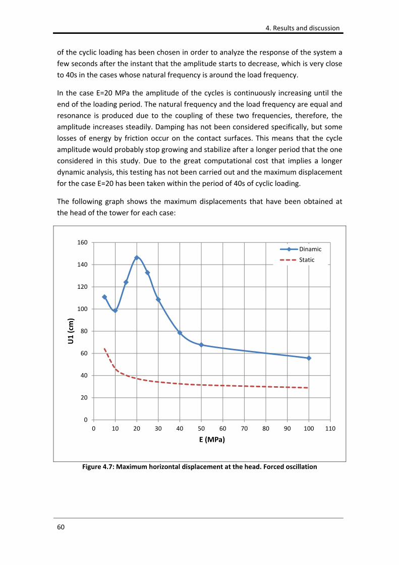
4. Results and discussion
60
of the cyclic loading has been chosen in order to analyze the response of the system a
few seconds after the instant that the amplitude starts to decrease, which is very close
to 40s in the cases whose natural frequency is around the load frequency.
In the case E=20 MPa the amplitude of the cycles is continuously increasing until the
end of the loading period. The natural frequency and the load frequency are equal and
resonance is produced due to the coupling of these two frequencies, therefore, the
amplitude increases steadily. Damping has not been considered specifically, but some
losses of energy by friction occur on the contact surfaces. This means that the cycle
amplitude would probably stop growing and stabilize after a longer period that the one
considered in this study. Due to the great computational cost that implies a longer
dynamic analysis, this testing has not been carried out and the maximum displacement
for the case E=20 has been taken within the period of 40s of cyclic loading.
The following graph shows the maximum displacements that have been obtained at
the head of the tower for each case:
Figure 4.7: Maximum horizontal displacement at the head. Forced oscillation
0
20
40
60
80
100
120
140
160
0 10 20 30 40 50 60 70 80 90 100 110
U1 (cm
)
E (MPa)
Dinamic
Static
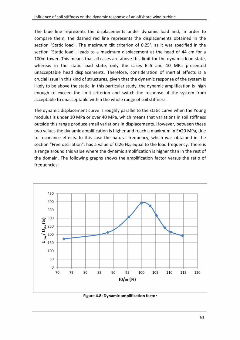
Influence of soil stiffness on the dynamic response of an offshore wind turbine
61
The blue line represents the displacements under dynamic load and, in order to
compare them, the dashed red line represents the displacements obtained in the
section "Static load". The maximum tilt criterion of 0.25°, as it was specified in the
section "Static load", leads to a maximum displacement at the head of 44 cm for a
100m tower. This means that all cases are above this limit for the dynamic load state,
whereas in the static load state, only the cases E=5 and 10 MPa presented
unacceptable head displacements. Therefore, consideration of inertial effects is a
crucial issue in this kind of structures, given that the dynamic response of the system is
likely to be above the static. In this particular study, the dynamic amplification is high
enough to exceed the limit criterion and switch the response of the system from
acceptable to unacceptable within the whole range of soil stiffness.
The dynamic displacement curve is roughly parallel to the static curve when the Young
modulus is under 10 MPa or over 40 MPa, which means that variations in soil stiffness
outside this range produce small variations in displacements. However, between these
two values the dynamic amplification is higher and reach a maximum in E=20 MPa, due
to resonance effects. In this case the natural frequency, which was obtained in the
section "Free oscillation", has a value of 0.26 Hz, equal to the load frequency. There is
a range around this value where the dynamic amplification is higher than in the rest of
the domain. The following graphs shows the amplification factor versus the ratio of
frequencies:
Figure 4.8: Dynamic amplification factor
0
50
100
150
200
250
300
350
400
450
70 75 80 85 90 95 100 105 110 115 120
Udin / U
sta(%
)
f0/ (%)
4. Results and discussion
62
Where:
Udin: Maximum displacement under cyclic load
Usta: Displacement under static load
f0: Natural frequency
: Load frequency. =0.263 Hz
The ratio f0/ ranges from 72% in the case E=5 MPa to 115% in the case E=100 MPa,
and there is dynamic amplification in all cases analyzed. The dynamic amplification
factor Udin/Usta reaches a maximum of 400% when the natural frequency is equal to the
load frequency. This factor decreases to 200% when the ratio f0/ is lower than 90% or higher than 110%. Increments of the ratio f0/ outside the range 90‐110% produce smaller variations of the amplification factor than those produced within this range.
Therefore, resonance effects are mainly produced when the ratio between natural
frequency and load frequency is 100% with an influence margin of 10%. This margin
of 10% around the load frequency is recommended by the code DNV (2014), which
suggests that the ranges of frequencies 1P and 3P to be avoided by the natural
frequency should be extended 10% at each end, P being the rotor frequency.
The displacement at the head of the tower, which has been analyzed above, is an
important factor in the Serviceability Limit State (SLS), but there are other limit states
that must be analyzed, as it was described in the section "Failure modes". Fatigue Limit
State (FLS) is critical in this kind of structures, due to the cyclic nature of loads, and the
stress range in the steel is the factor that determines this model of failure. The
following figure shows a stress contour of the tower for the case E=20 MPa:
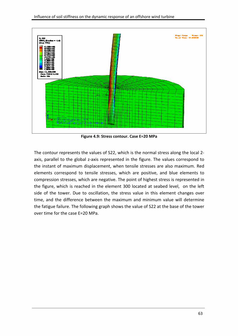
Influence of soil stiffness on the dynamic response of an offshore wind turbine
63
Figure 4.9: Stress contour. Case E=20 MPa
The contour represents the values of S22, which is the normal stress along the local 2‐
axis, parallel to the global z‐axis represented in the figure. The values correspond to
the instant of maximum displacement, when tensile stresses are also maximum. Red
elements correspond to tensile stresses, which are positive, and blue elements to
compression stresses, which are negative. The point of highest stress is represented in
the figure, which is reached in the element 300 located at seabed level, on the left
side of the tower. Due to oscillation, the stress value in this element changes over
time, and the difference between the maximum and minimum value will determine
the fatigue failure. The following graph shows the value of S22 at the base of the tower
over time for the case E=20 MPa.
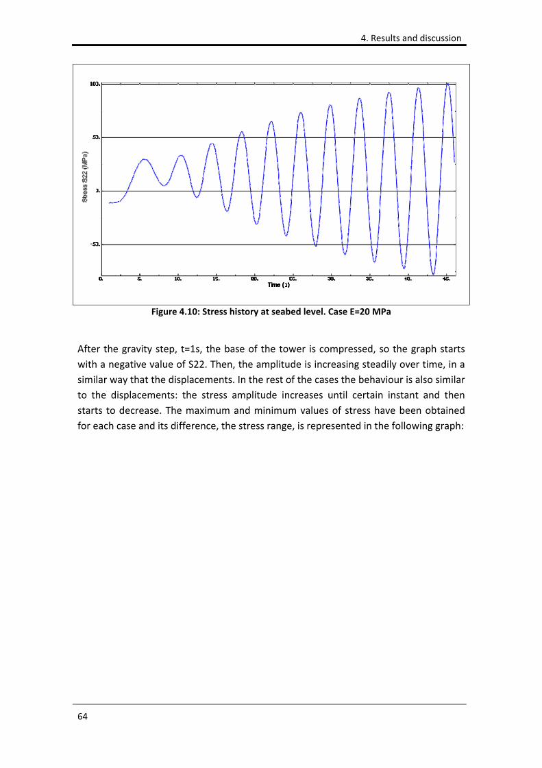
4. Results and discussion
64
Figure 4.10: Stress history at seabed level. Case E=20 MPa
After the gravity step, t=1s, the base of the tower is compressed, so the graph starts
with a negative value of S22. Then, the amplitude is increasing steadily over time, in a
similar way that the displacements. In the rest of the cases the behaviour is also similar
to the displacements: the stress amplitude increases until certain instant and then
starts to decrease. The maximum and minimum values of stress have been obtained
for each case and its difference, the stress range, is represented in the following graph:
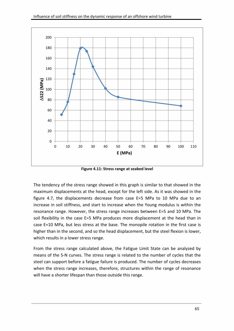
Influence of soil stiffness on the dynamic response of an offshore wind turbine
65
Figure 4.11: Stress range at seabed level
The tendency of the stress range showed in this graph is similar to that showed in the
maximum displacements at the head, except for the left side. As it was showed in the
figure 4.7, the displacements decrease from case E=5 MPa to 10 MPa due to an
increase in soil stiffness, and start to increase when the Young modulus is within the
resonance range. However, the stress range increases between E=5 and 10 MPa. The
soil flexibility in the case E=5 MPa produces more displacement at the head than in
case E=10 MPa, but less stress at the base. The monopile rotation in the first case is
higher than in the second, and so the head displacement, but the steel flexion is lower,
which results in a lower stress range.
From the stress range calculated above, the Fatigue Limit State can be analyzed by
means of the S‐N curves. The stress range is related to the number of cycles that the
steel can support before a fatigue failure is produced. The number of cycles decreases
when the stress range increases, therefore, structures within the range of resonance
will have a shorter lifespan than those outside this range.
0
20
40
60
80
100
120
140
160
180
200
0 10 20 30 40 50 60 70 80 90 100 110
S22 (MPa)
E (MPa)
4. Results and discussion
66
4.4 P‐yandM‐curves
A static analysis has been performed in the model in order to obtain the P‐y and M‐ curves. These curves represent the stiffness of the system soil‐foundation and are
formed by the following parameters:
P: Horizontal reaction force at the base of the tower
y: Horizontal displacement at the base of the towe
M: Reaction moment at the base of the tower
: Angle of rotation at the base of the tower
A horizontal force F is applied at the head of the tower to obtain these four
parameters. Each curve has been defined with 9 points, in addition to the (0,0) point,
which have been calculated from 9 equilibrium states with different values of F. The
magnitude of F ranges from 0 to 4000 kN, leading to head displacements from 0 to
2.72m. Values of F over 4000 kN have been tested but not included, because they
produce excessive plastic strain around the pile and some convergence problems arise.
Moreover, head displacements higher than 2.72m are well above the range that have
been analyzed in this study. The maximum head displacement obtained in previous
analyses is 1.46m, as it is shown in the figure 4.7. Therefore, a maximum force of
4000kN is enough to define the stiffness curves of the foundation in this case.
The analysis of the stiffness curves has been focused only on the case E=20 MPa, due
to the high computational cost that it requires. There are two curves to obtain for each
case, each of them needs to be defined by 9 points. Each equilibrium state gives a
point for each curve, so it would be necessary to perform 81 equilibrium states to
obtain the curves of the 9 cases. The case E=20 MPa is considered to be representative
to analyze the modelling issues associated with stiffness curves.
The two following graphs represent the P‐y and M‐ curves which have been obtained according to the methodology detailed above:
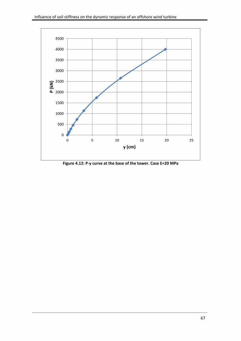
Influence of soil stiffness on the dynamic response of an offshore wind turbine
67
Figure 4.12: P‐y curve at the base of the tower. Case E=20 MPa
0
500
1000
1500
2000
2500
3000
3500
4000
4500
0 5 10 15 20 25
P (kN
)
y (cm)
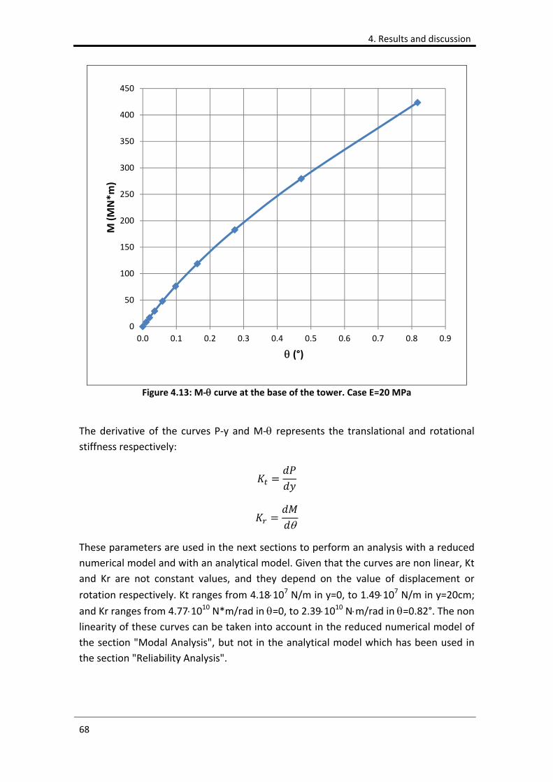
4. Results and discussion
68
Figure 4.13: M‐ curve at the base of the tower. Case E=20 MPa
The derivative of the curves P‐y and M‐ represents the translational and rotational stiffness respectively:
These parameters are used in the next sections to perform an analysis with a reduced
numerical model and with an analytical model. Given that the curves are non linear, Kt
and Kr are not constant values, and they depend on the value of displacement or
rotation respectively. Kt ranges from 4.18107 N/m in y=0, to 1.49107 N/m in y=20cm;
and Kr ranges from 4.771010 N*m/rad in =0, to 2.391010 Nm/rad in =0.82°. The non linearity of these curves can be taken into account in the reduced numerical model of
the section "Modal Analysis", but not in the analytical model which has been used in
the section "Reliability Analysis".
0
50
100
150
200
250
300
350
400
450
0.0 0.1 0.2 0.3 0.4 0.5 0.6 0.7 0.8 0.9
M (MN*m
)
(°)
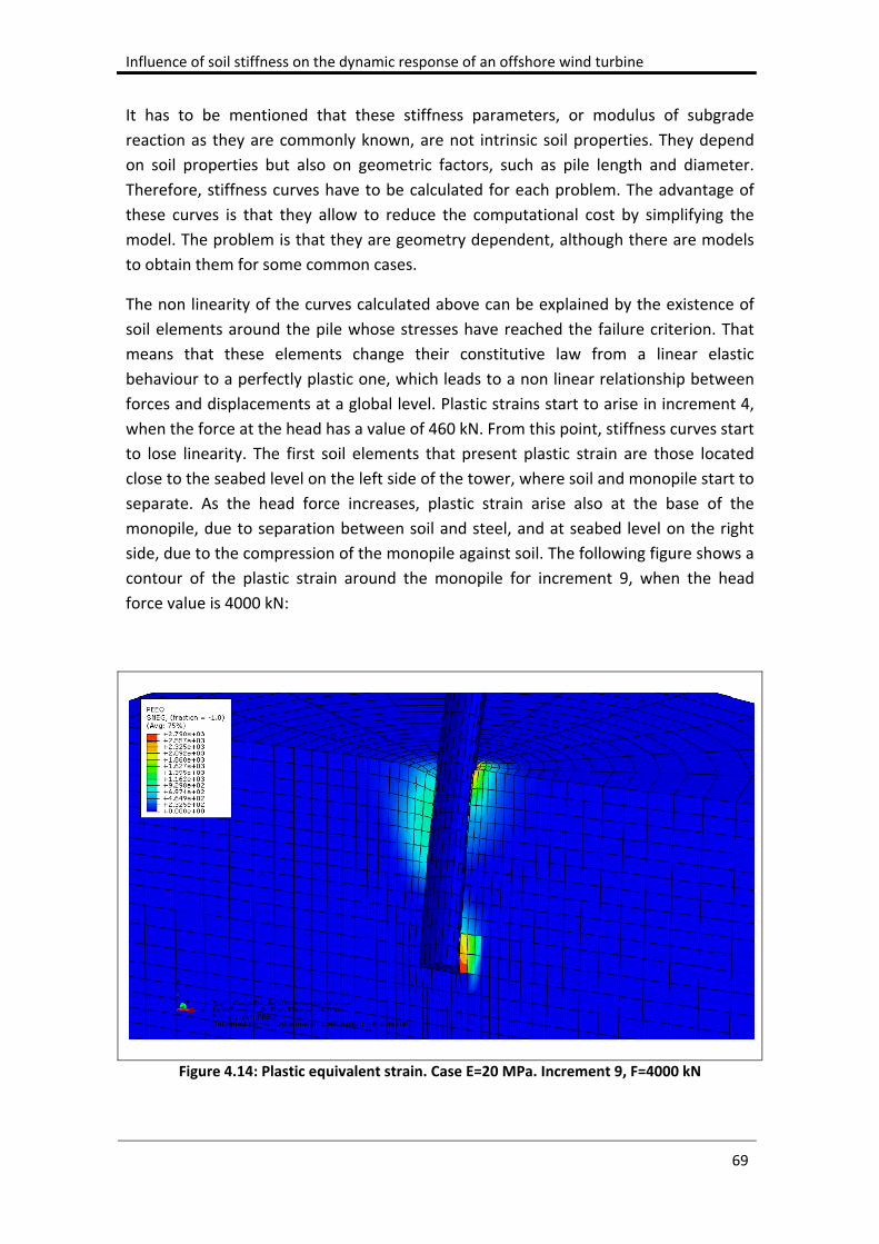
Influence of soil stiffness on the dynamic response of an offshore wind turbine
69
It has to be mentioned that these stiffness parameters, or modulus of subgrade
reaction as they are commonly known, are not intrinsic soil properties. They depend
on soil properties but also on geometric factors, such as pile length and diameter.
Therefore, stiffness curves have to be calculated for each problem. The advantage of
these curves is that they allow to reduce the computational cost by simplifying the
model. The problem is that they are geometry dependent, although there are models
to obtain them for some common cases.
The non linearity of the curves calculated above can be explained by the existence of
soil elements around the pile whose stresses have reached the failure criterion. That
means that these elements change their constitutive law from a linear elastic
behaviour to a perfectly plastic one, which leads to a non linear relationship between
forces and displacements at a global level. Plastic strains start to arise in increment 4,
when the force at the head has a value of 460 kN. From this point, stiffness curves start
to lose linearity. The first soil elements that present plastic strain are those located
close to the seabed level on the left side of the tower, where soil and monopile start to
separate. As the head force increases, plastic strain arise also at the base of the
monopile, due to separation between soil and steel, and at seabed level on the right
side, due to the compression of the monopile against soil. The following figure shows a
contour of the plastic strain around the monopile for increment 9, when the head
force value is 4000 kN:
Figure 4.14: Plastic equivalent strain. Case E=20 MPa. Increment 9, F=4000 kN
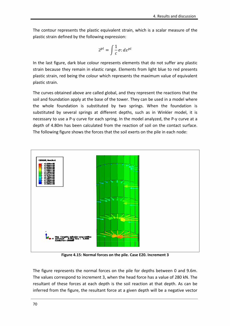
4. Results and discussion
70
The contour represents the plastic equivalent strain, which is a scalar measure of the
plastic strain defined by the following expression:
1
:
In the last figure, dark blue colour represents elements that do not suffer any plastic
strain because they remain in elastic range. Elements from light blue to red presents
plastic strain, red being the colour which represents the maximum value of equivalent
plastic strain.
The curves obtained above are called global, and they represent the reactions that the
soil and foundation apply at the base of the tower. They can be used in a model where
the whole foundation is substituted by two springs. When the foundation is
substituted by several springs at different depths, such as in Winkler model, it is
necessary to use a P‐y curve for each spring. In the model analyzed, the P‐y curve at a
depth of 4.80m has been calculated from the reaction of soil on the contact surface.
The following figure shows the forces that the soil exerts on the pile in each node:
Figure 4.15: Normal forces on the pile. Case E20. Increment 3
The figure represents the normal forces on the pile for depths between 0 and 9.6m.
The values correspond to increment 3, when the head force has a value of 280 kN. The
resultant of these forces at each depth is the soil reaction at that depth. As can be
inferred from the figure, the resultant force at a given depth will be a negative vector
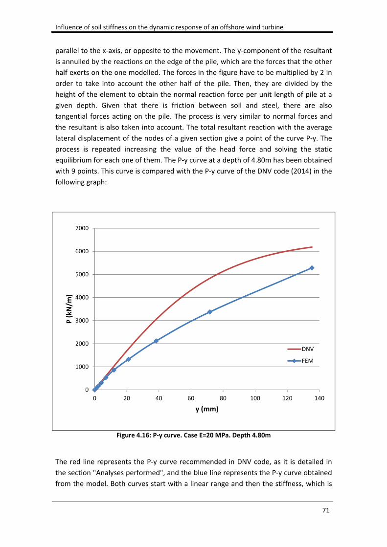
Influence of soil stiffness on the dynamic response of an offshore wind turbine
71
parallel to the x‐axis, or opposite to the movement. The y‐component of the resultant
is annulled by the reactions on the edge of the pile, which are the forces that the other
half exerts on the one modelled. The forces in the figure have to be multiplied by 2 in
order to take into account the other half of the pile. Then, they are divided by the
height of the element to obtain the normal reaction force per unit length of pile at a
given depth. Given that there is friction between soil and steel, there are also
tangential forces acting on the pile. The process is very similar to normal forces and
the resultant is also taken into account. The total resultant reaction with the average
lateral displacement of the nodes of a given section give a point of the curve P‐y. The
process is repeated increasing the value of the head force and solving the static
equilibrium for each one of them. The P‐y curve at a depth of 4.80m has been obtained
with 9 points. This curve is compared with the P‐y curve of the DNV code (2014) in the
following graph:
Figure 4.16: P‐y curve. Case E=20 MPa. Depth 4.80m
The red line represents the P‐y curve recommended in DNV code, as it is detailed in
the section "Analyses performed", and the blue line represents the P‐y curve obtained
from the model. Both curves start with a linear range and then the stiffness, which is
0
1000
2000
3000
4000
5000
6000
7000
0 20 40 60 80 100 120 140
P (kN
/m)
y (mm)
DNV
FEM
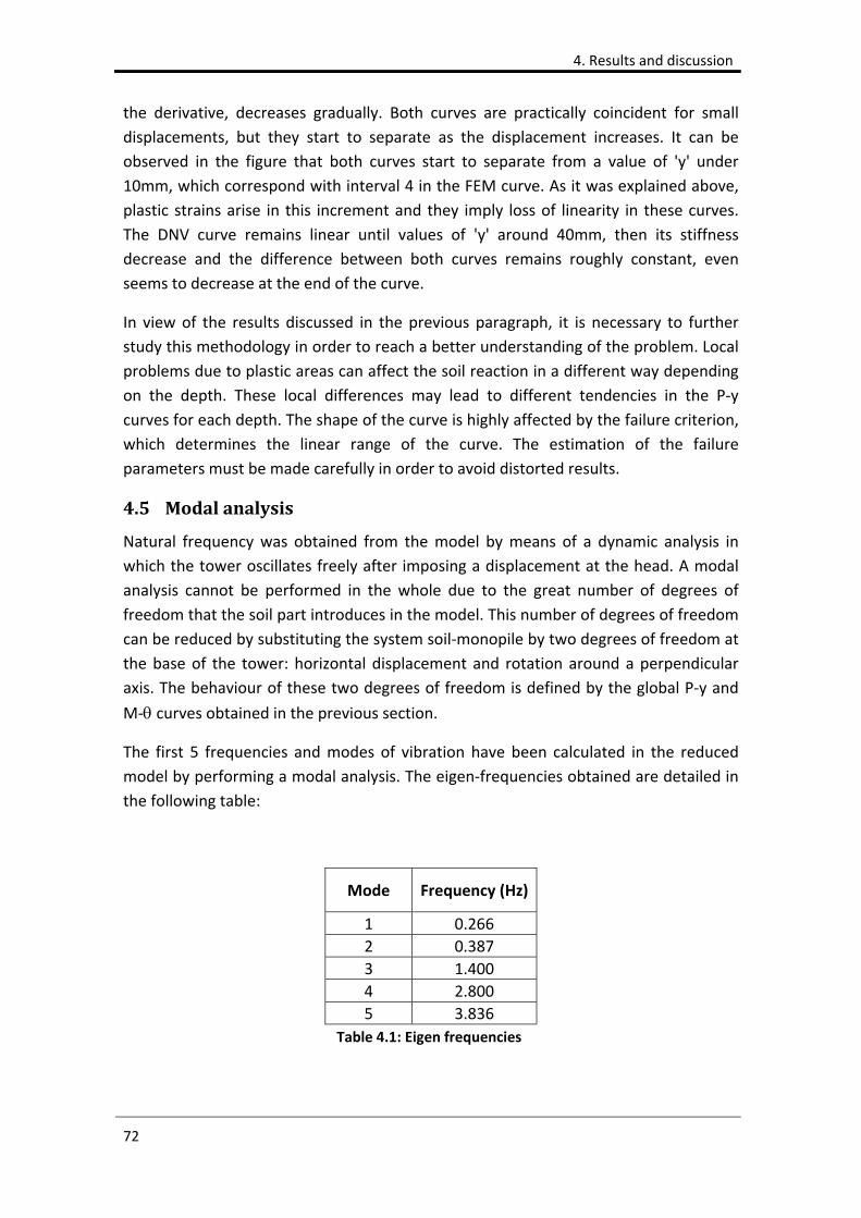
4. Results and discussion
72
the derivative, decreases gradually. Both curves are practically coincident for small
displacements, but they start to separate as the displacement increases. It can be
observed in the figure that both curves start to separate from a value of 'y' under
10mm, which correspond with interval 4 in the FEM curve. As it was explained above,
plastic strains arise in this increment and they imply loss of linearity in these curves.
The DNV curve remains linear until values of 'y' around 40mm, then its stiffness
decrease and the difference between both curves remains roughly constant, even
seems to decrease at the end of the curve.
In view of the results discussed in the previous paragraph, it is necessary to further
study this methodology in order to reach a better understanding of the problem. Local
problems due to plastic areas can affect the soil reaction in a different way depending
on the depth. These local differences may lead to different tendencies in the P‐y
curves for each depth. The shape of the curve is highly affected by the failure criterion,
which determines the linear range of the curve. The estimation of the failure
parameters must be made carefully in order to avoid distorted results.
4.5 Modalanalysis
Natural frequency was obtained from the model by means of a dynamic analysis in
which the tower oscillates freely after imposing a displacement at the head. A modal
analysis cannot be performed in the whole due to the great number of degrees of
freedom that the soil part introduces in the model. This number of degrees of freedom
can be reduced by substituting the system soil‐monopile by two degrees of freedom at
the base of the tower: horizontal displacement and rotation around a perpendicular
axis. The behaviour of these two degrees of freedom is defined by the global P‐y and
M‐ curves obtained in the previous section.
The first 5 frequencies and modes of vibration have been calculated in the reduced
model by performing a modal analysis. The eigen‐frequencies obtained are detailed in
the following table:
Mode Frequency (Hz)
1 0.266
2 0.387
3 1.400
4 2.800
5 3.836
Table 4.1: Eigen frequencies
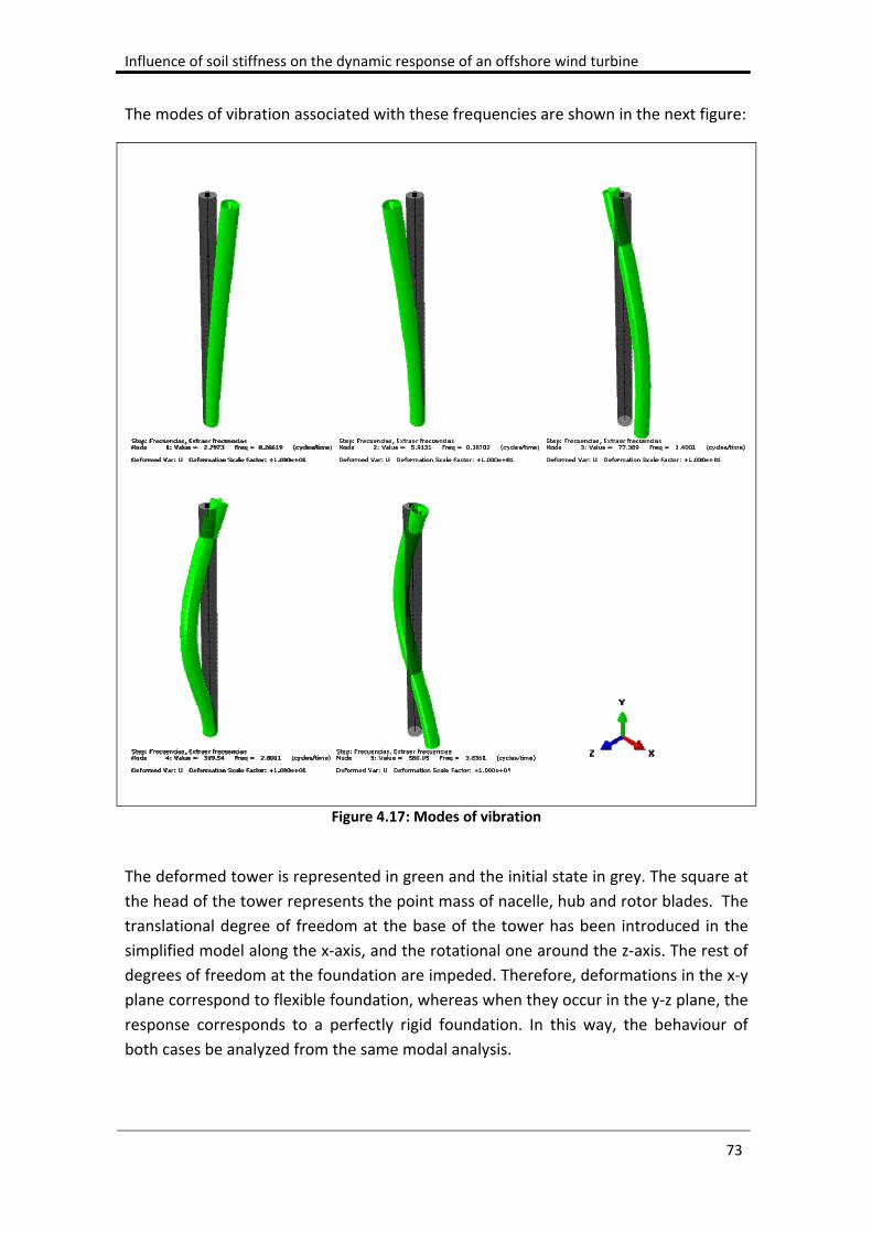
Influence of soil stiffness on the dynamic response of an offshore wind turbine
73
The modes of vibration associated with these frequencies are shown in the next figure:
Figure 4.17: Modes of vibration
The deformed tower is represented in green and the initial state in grey. The square at
the head of the tower represents the point mass of nacelle, hub and rotor blades. The
translational degree of freedom at the base of the tower has been introduced in the
simplified model along the x‐axis, and the rotational one around the z‐axis. The rest of
degrees of freedom at the foundation are impeded. Therefore, deformations in the x‐y
plane correspond to flexible foundation, whereas when they occur in the y‐z plane, the
response corresponds to a perfectly rigid foundation. In this way, the behaviour of
both cases be analyzed from the same modal analysis.
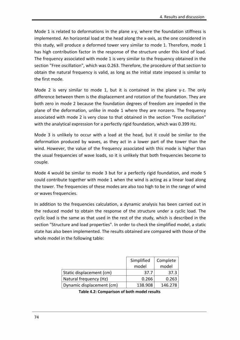
4. Results and discussion
74
Mode 1 is related to deformations in the plane x‐y, where the foundation stiffness is
implemented. An horizontal load at the head along the x‐axis, as the one considered in
this study, will produce a deformed tower very similar to mode 1. Therefore, mode 1
has high contribution factor in the response of the structure under this kind of load.
The frequency associated with mode 1 is very similar to the frequency obtained in the
section "Free oscillation", which was 0.263. Therefore, the procedure of that section to
obtain the natural frequency is valid, as long as the initial state imposed is similar to
the first mode.
Mode 2 is very similar to mode 1, but it is contained in the plane y‐z. The only
difference between them is the displacement and rotation of the foundation. They are
both zero in mode 2 because the foundation degrees of freedom are impeded in the
plane of the deformation, unlike in mode 1 where they are nonzero. The frequency
associated with mode 2 is very close to that obtained in the section "Free oscillation"
with the analytical expression for a perfectly rigid foundation, which was 0.399 Hz.
Mode 3 is unlikely to occur with a load at the head, but it could be similar to the
deformation produced by waves, as they act in a lower part of the tower than the
wind. However, the value of the frequency associated with this mode is higher than
the usual frequencies of wave loads, so it is unlikely that both frequencies become to
couple.
Mode 4 would be similar to mode 3 but for a perfectly rigid foundation, and mode 5
could contribute together with mode 1 when the wind is acting as a linear load along
the tower. The frequencies of these modes are also too high to be in the range of wind
or waves frequencies.
In addition to the frequencies calculation, a dynamic analysis has been carried out in
the reduced model to obtain the response of the structure under a cyclic load. The
cyclic load is the same as that used in the rest of the study, which is described in the
section "Structure and load properties". In order to check the simplified model, a static
state has also been implemented. The results obtained are compared with those of the
whole model in the following table:
Simplified model
Complete model
Static displacement (cm) 37.7 37.3
Natural frequency (Hz) 0.266 0.263
Dynamic displacement (cm) 138.908 146.278
Table 4.2: Comparison of both model results
Influence of soil stiffness on the dynamic response of an offshore wind turbine
75
As it was expected, there is good agreement between the static displacements in both
models, given that the P‐y and M‐ curves implemented in the simplified model were
obtained from a static analysis. However, the dynamic displacements do not agree so
well, the difference between them being of more than 7 cm. When inertial effects are
relevant, parameters such as stiffness of the foundation or damping must be chosen
carefully. In this case, the static stiffness curves do not approximate well the response
of the system soil‐foundation when cyclic loading is involved. On the other hand, the
natural frequencies calculated with both methodologies are practically the same. As
the modal analysis of eigenvalues does not involve large displacements, inertial effects
do not affect so much the results and the static curves are valid to simulate the system
soil‐foundation.
4.6 Reliabilityanalysis
In this section, the natural frequency has been calculated from an analytical model
where translational and rotational stiffness, Kt and Kr respectively, have been
considered as stochastic variables. The mean values of these variables have been
obtained from the global stiffness curves calculated in the section "P‐y and M‐ curves". As the curves are non linear, increment 7 has been chosen as representative,
because the displacement at the head in this increment is within the range of that
caused by the load of the problem. Then, the stochastic variables are characterized as
follows:
KtlogN(mean=2.37*107 N/m, COV=0.3)
KrlogN(mean=3.30*1010 N*m/rad, COV=0.2)
Before starting the analysis it is necessary to obtain the parameters that define the
probability density functions of Kr and Kt, that is, and . These are the following for a lognormal distribution:
√
1
Where:
: Location parameter
: Scale parameter
m: Mean of the non logarithmic sample values
s: Variance of the non logarithmic sample values. ∙
4. Results and discussion
76
The values obtained from the equations above are the following:
r=24.200 , r=0.198 , t=16.938 , t=0.294
The result of the analysis will be the probability that the natural frequency is within the
range of resonance of a load frequency. As it was discussed in the section "Forced
oscillation", there is a range of 10% around the load frequency that has to be avoided
by the natural frequency in order to prevent resonance. Therefore, the probability that
the natural frequency of the system is in the range of 10% around a given load frequency is going to be calculated.
Given that the mean values of Kt and Kr are calculated from the case E=20, whose
natural frequency is equal to the load frequency considered in the previous analyses,
the probability that they are in the range of resonance would be almost 100%. In this
section, a different load frequency will be considered in order to evaluate the
probability of resonance when the mean values of natural and load frequencies are
slightly far. Then, the load frequency considered in this section is the following:
Load frequency: =0.22 Hz
Range of resonance (10%): 0.20 ‐ 0.24 Hz
4.6.1 Montecarlo
The Montecarlo method is based on computing a large number of simulations for
different realizations of the stochastic variables. This values are taken randomly, so the
number of simulations has to be large enough to cover a representative range of
events (Metropolis & Ulam, 1949). The steps of the method are the following:
Fix a number of simulations, n.
Compute two series of n uniformly distributed values ranging between 0 and 1: Nr and Nt.
Each pair of values Nr and Nt is related to a pair of values Kr and Kt. These can be obtained from the inverse cumulative distribution function of each one. In this case we obtain two series of values for Kr and Kt with a log normal distribution.
Compute the non dimensional parameters associated with each pair of values Kr and Kt:
Influence of soil stiffness on the dynamic response of an offshore wind turbine
77
Solve the equation of the natural frequency. It has to be done numerically for each pair of values Kr and Kt using the Newton‐Raphson method. The root of the equation associated with the natural frequency is that which is closest to
zero and positive. This root is the non dimensional frequency 1:
| | 0 1
Compute the natural frequency:
12
∙
Compute the probability of failure, which in this case is the probability of resonance, by counting the number of events:
1
Where:
n1: Number of events in which (0.9*) < f1 < (1.1*)
The results presented are obtained after 7000 simulations, from which the following
results have been obtained:
Total simulations: n=7000
Failure events: n1=714
Probability of resonance: Pf=10.20%
Computational cost: 7000
From these results we can see that there is a probability of 10.20% that the natural
frequency of the structure will be within the resonance range of the studied load,
which will cause dynamic amplification problems. As we can see in the table 4.3 below,
the mean value of the sample is 0.262 Hz, which is higher than the frequency load 0.22
Hz. The probability of failure can be reduced by designing a stiffer foundation, which
will result in an increase in the mean value of the natural frequency and a reduction in
the number of events within the range of resonance. The analysed design could be
dangerous if the soil had a strain softening behaviour, which would cause a decrease in
the natural frequency and, therefore, an increase in the probability of failure.
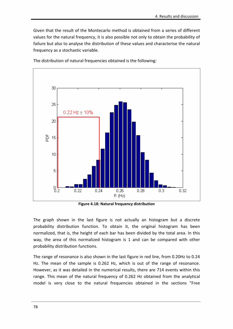
4. Results and discussion
78
Given that the result of the Montecarlo method is obtained from a series of different
values for the natural frequency, it is also possible not only to obtain the probability of
failure but also to analyse the distribution of these values and characterise the natural
frequency as a stochastic variable.
The distribution of natural frequencies obtained is the following:
Figure 4.18: Natural frequency distribution
The graph shown in the last figure is not actually an histogram but a discrete
probability distribution function. To obtain it, the original histogram has been
normalized, that is, the height of each bar has been divided by the total area. In this
way, the area of this normalized histogram is 1 and can be compared with other
probability distribution functions.
The range of resonance is also shown in the last figure in red line, from 0.20Hz to 0.24
Hz. The mean of the sample is 0.262 Hz, which is out of the range of resonance.
However, as it was detailed in the numerical results, there are 714 events within this
range. This mean of the natural frequency of 0.262 Hz obtained from the analytical
model is very close to the natural frequencies obtained in the sections "Free
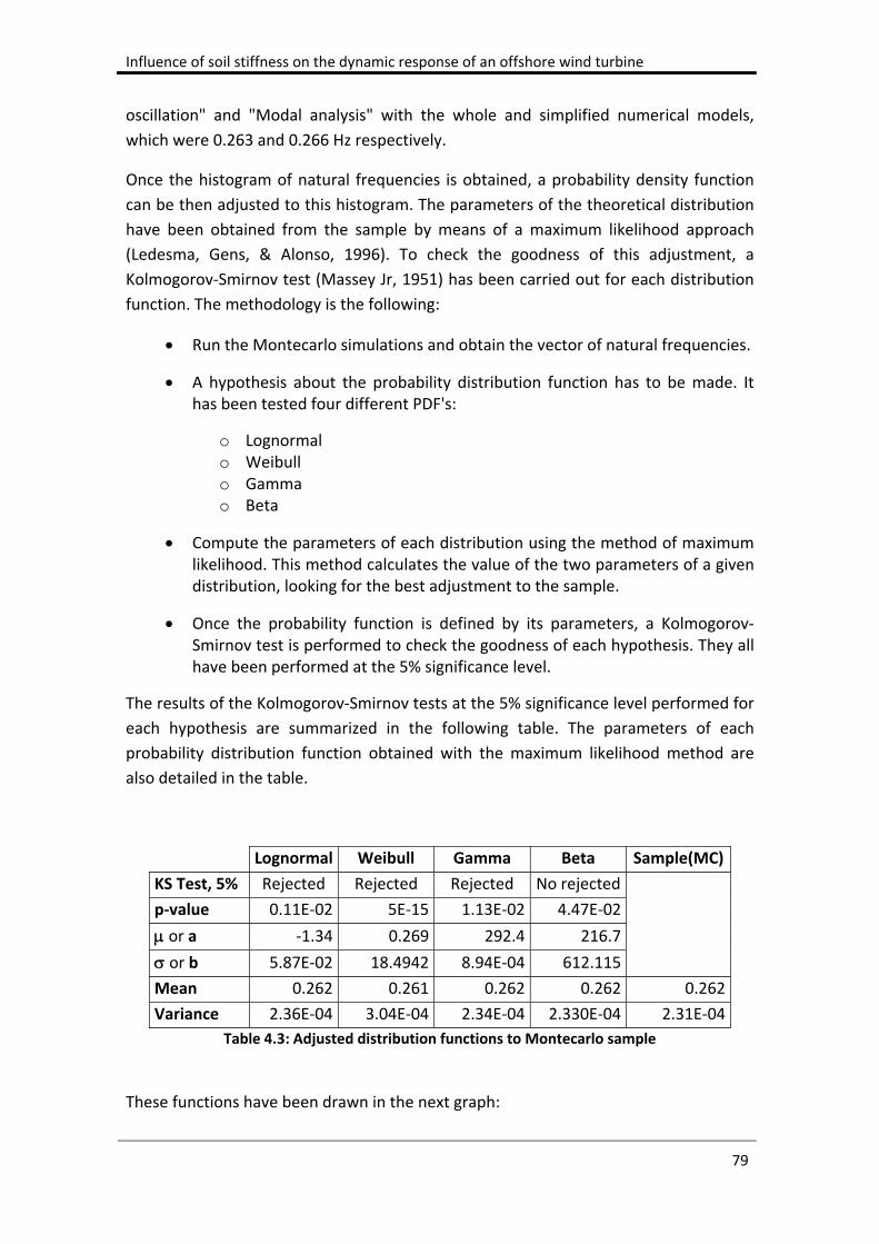
Influence of soil stiffness on the dynamic response of an offshore wind turbine
79
oscillation" and "Modal analysis" with the whole and simplified numerical models,
which were 0.263 and 0.266 Hz respectively.
Once the histogram of natural frequencies is obtained, a probability density function
can be then adjusted to this histogram. The parameters of the theoretical distribution
have been obtained from the sample by means of a maximum likelihood approach
(Ledesma, Gens, & Alonso, 1996). To check the goodness of this adjustment, a
Kolmogorov‐Smirnov test (Massey Jr, 1951) has been carried out for each distribution
function. The methodology is the following:
Run the Montecarlo simulations and obtain the vector of natural frequencies.
A hypothesis about the probability distribution function has to be made. It has been tested four different PDF's:
o Lognormal o Weibull o Gamma o Beta
Compute the parameters of each distribution using the method of maximum likelihood. This method calculates the value of the two parameters of a given distribution, looking for the best adjustment to the sample.
Once the probability function is defined by its parameters, a Kolmogorov‐Smirnov test is performed to check the goodness of each hypothesis. They all have been performed at the 5% significance level.
The results of the Kolmogorov‐Smirnov tests at the 5% significance level performed for
each hypothesis are summarized in the following table. The parameters of each
probability distribution function obtained with the maximum likelihood method are
also detailed in the table.
Lognormal Weibull Gamma Beta Sample(MC)
KS Test, 5% Rejected Rejected Rejected No rejected
p‐value 0.11E‐02 5E‐15 1.13E‐02 4.47E‐02
or a ‐1.34 0.269 292.4 216.7
or b 5.87E‐02 18.4942 8.94E‐04 612.115
Mean 0.262 0.261 0.262 0.262 0.262
Variance 2.36E‐04 3.04E‐04 2.34E‐04 2.330E‐04 2.31E‐04
Table 4.3: Adjusted distribution functions to Montecarlo sample
These functions have been drawn in the next graph:

4. Results and discussion
80
Figure 4.19: Tested distribution functions
The graph shows that the Lognormal, Gamma and Beta distributions are very close and
practically overlapped, whereas the Weibull distribution is far from the rest. Attending
to the numerical results of the table, the only hypothesis which has not been rejected
by the Kolmogorov‐Smirnov test is that the sample follows a Beta distribution. The p‐
value shown in the table is related to the probability that the theoretical function
adjust to the sample, and it allows to compare the different hypothesis. High values of
this parameter indicate a better fit than lower values. The p‐value is close in the
Gamma and Beta distributions, slightly higher in this last. The little difference between
these two values and the fact that the test rejects only one of them indicates that the
adjustment of the Beta distribution, although it has not been rejected, is in the limit of
rejection. In the case of the Weibull distribution, the p‐value is far from the other
three, and it can be seen in the graph that the function is too right skewed.
Attending to the statistics values, mean and variance, obtained by the maximum
likelihood method, it can be seen that they are very similar and close to the values
obtained from the sample, that is, from the results of the simulations. However, the
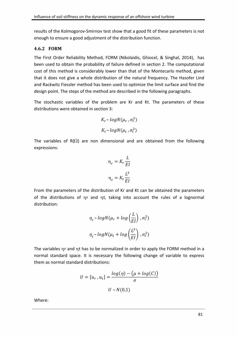
Influence of soil stiffness on the dynamic response of an offshore wind turbine
81
results of the Kolmogorov‐Smirnov test show that a good fit of these parameters is not
enough to ensure a good adjustment of the distribution function.
4.6.2 FORM
The First Order Reliability Method, FORM (Nikolaidis, Ghiocel, & Singhal, 2014), has
been used to obtain the probability of failure defined in section 2. The computational
cost of this method is considerably lower than that of the Montecarlo method, given
that it does not give a whole distribution of the natural frequency. The Hasofer Lind
and Rackwitz Fiessler method has been used to optimize the limit surface and find the
design point. The steps of the method are described in the following paragraphs.
The stochastic variables of the problem are Kr and Kt. The parameters of these
distributions were obtained in section 3:
,
,
The variables of R() are non dimensional and are obtained from the following
expressions:
From the parameters of the distribution of Kr and Kt can be obtained the parameters
of the distributions of r and t, taking into account the rules of a lognormal
distribution:
,
,
The variables r and t has to be normalized in order to apply the FORM method in a
normal standard space. It is necessary the following change of variable to express
them as normal standard distributions:
,
0,1
Where:
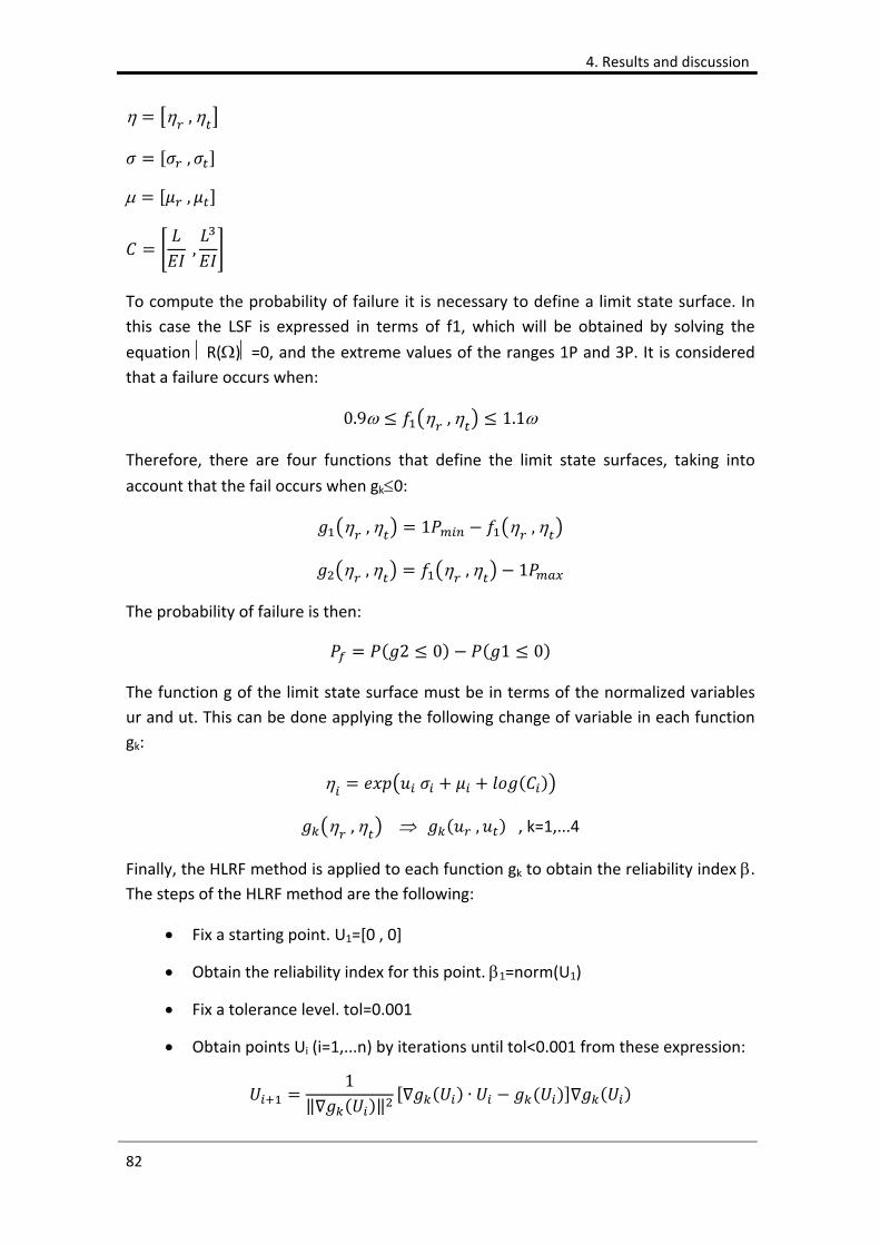
4. Results and discussion
82
,
,
,
,
To compute the probability of failure it is necessary to define a limit state surface. In
this case the LSF is expressed in terms of f1, which will be obtained by solving the
equation R()=0, and the extreme values of the ranges 1P and 3P. It is considered
that a failure occurs when:
0.9 , 1.1
Therefore, there are four functions that define the limit state surfaces, taking into
account that the fail occurs when gk0:
, 1 ,
, , 1
The probability of failure is then:
2 0 1 0
The function g of the limit state surface must be in terms of the normalized variables
ur and ut. This can be done applying the following change of variable in each function
gk:
, , , k=1,...4
Finally, the HLRF method is applied to each function gk to obtain the reliability index . The steps of the HLRF method are the following:
Fix a starting point. U1=[0 , 0]
Obtain the reliability index for this point. 1=norm(U1)
Fix a tolerance level. tol=0.001
Obtain points Ui (i=1,...n) by iterations until tol<0.001 from these expression:
1‖ ‖
∙
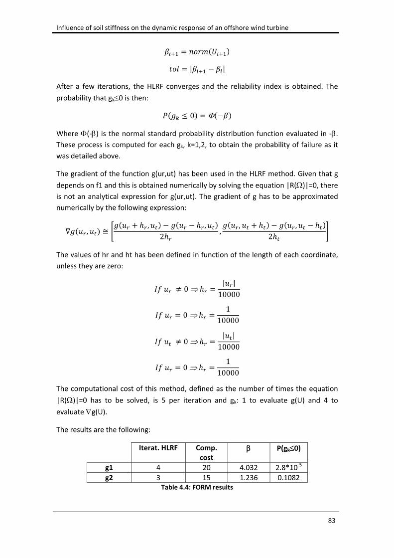
Influence of soil stiffness on the dynamic response of an offshore wind turbine
83
| |
After a few iterations, the HLRF converges and the reliability index is obtained. The
probability that gk0 is then:
0
Where (‐) is the normal standard probability distribution function evaluated in ‐. These process is computed for each gk, k=1,2, to obtain the probability of failure as it
was detailed above.
The gradient of the function g(ur,ut) has been used in the HLRF method. Given that g
depends on f1 and this is obtained numerically by solving the equation |R()|=0, there is not an analytical expression for g(ur,ut). The gradient of g has to be approximated
numerically by the following expression:
, ≅, ,
2,
, ,2
The values of hr and ht has been defined in function of the length of each coordinate,
unless they are zero:
0| |10000
01
10000
0| |10000
01
10000
The computational cost of this method, defined as the number of times the equation
|R()|=0 has to be solved, is 5 per iteration and gk: 1 to evaluate g(U) and 4 to evaluate g(U).
The results are the following:
Iterat. HLRF Comp. cost
P(gk0)
g1 4 20 4.032 2.8*10‐5
g2 3 15 1.236 0.1082 Table 4.4: FORM results
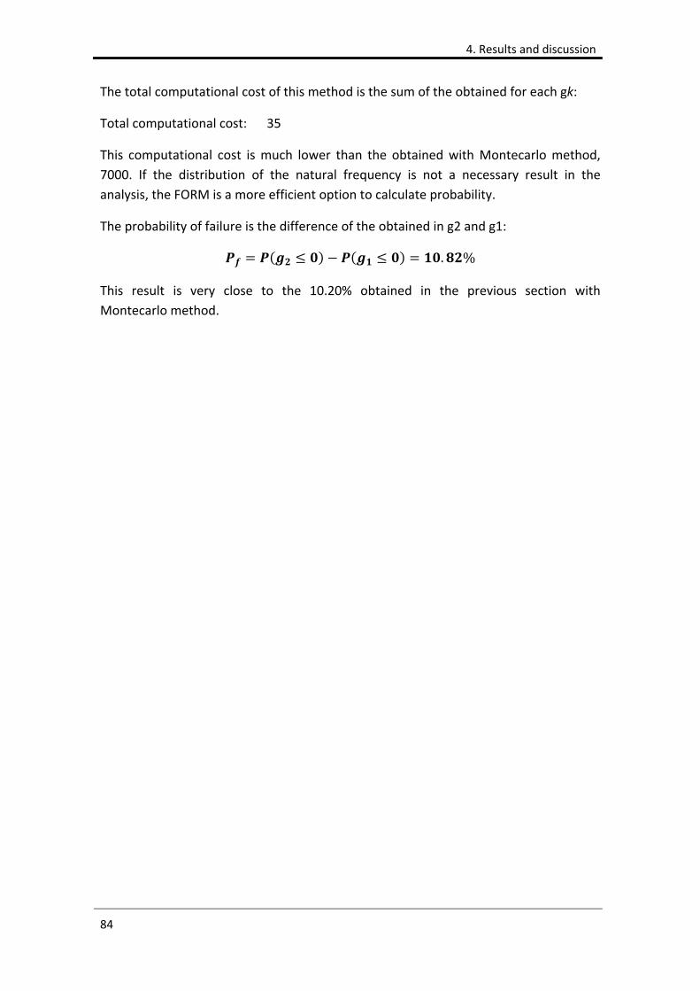
4. Results and discussion
84
The total computational cost of this method is the sum of the obtained for each gk:
Total computational cost: 35
This computational cost is much lower than the obtained with Montecarlo method,
7000. If the distribution of the natural frequency is not a necessary result in the
analysis, the FORM is a more efficient option to calculate probability.
The probability of failure is the difference of the obtained in g2 and g1:
. %
This result is very close to the 10.20% obtained in the previous section with
Montecarlo method.
Influence of soil stiffness on the dynamic response of an offshore wind turbine
85
5 Conclusions
Several analyses have been carried out in this study to analyze the influence of soil
properties on the response of an offshore wind turbine on a monopile foundation. A
finite element model has been implemented in which the soil is represented as a
continuous element with a Mohr‐Coulomb failure criterion. This model has been used
as a tool to obtain the response of the tower under several load states: static, free
oscillation and forced oscillation. P‐y and M‐ curves at the base of the tower have also been calculated from the model. These curves have been implemented in a
reduced model in which the system soil‐foundation is substituted by two degrees of
freedom at the base of the tower: horizontal translation and rotation. The behaviour
of these two degrees of freedom is determined by the P‐y and M‐ curves. A modal
analysis has been performed in the reduced model to obtain the vibration modes of
the system and its frequencies. Finally, a reliability analysis has been performed to
obtain the probability of resonance. In this analysis, translational and rotational
stiffness are considered as stochastic variables. The probability of resonance has been
calculated with two different methods: Montecarlo and FORM.
The results from the static analysis show that the head displacement decreases when
the soil stiffness increases. The curve of displacement tends to the value of a perfectly
rigid foundation, although the difference in the stiffest case is still considerable,
around 34%. The influence of soil stiffness is higher in the case of loose sands, where
small increments of stiffness lead to large increments in displacement.
Soil stiffness also affects the natural frequency of the system, as it is shown in the
results of the free oscillation analysis. As the soil stiffness increases, the natural
frequency is higher. There is a trend to the frequency of the perfectly rigid foundation,
but the difference between them is around 33% in the stiffest case. Again, the
influence of soil stiffness on natural frequency is higher in loose sands. In the case of
dense sands, the increments in natural frequency are very small when soil stiffness
increases.
The forced oscillation results show that dynamic amplification has been produced in all
cases, although it is much more relevant around the resonance range. The natural
frequency of the system has ranged from 72 to 115% of the load frequency. Within this
range, the dynamic amplification has been always higher than 175%, and has reached
a maximum of almost 400% when the natural frequency equals the load frequency.
There is a range of 10% around the load frequency where the amplification factor
starts to increase sharply. The steel stress range at the base of the tower, which
determines the fatigue life of the structure, has shown a similar behaviour to the
displacements. This stress range increases sharply when the natural frequency of the
system is within the interval of 10% around the load frequency.
5. Conclusions
86
The global P‐y and M‐ curves obtained from the incremental static analysis show a
range of linear behaviour when the displacements and rotations are small. The point
from which the slope of the curves starts to decrease coincides with the beginning of
plastic strain in elements around the pile. These plastic strains start to arise close to
the seabed level, on the side where the monopile separates from the soil. As the load
increases, they extend to the opposite side, due to compression in soil produced by
the monopile, and they also arise at the monopile tip, where the soil separates from
steel due to rotation.
The first five modes of vibration have been calculated from a modal analysis in the
reduced model. The first mode is the most influential in the response of the structure
under a horizontal load. Therefore, the first frequency of the system, or natural
frequency, can get coupled with the frequency of a horizontal load and produce
resonance. Attending to the shape of the third mode, it could be excited by wave
loads, as they are applied at a lower point. However, it is unlikely that frequency of the
third vibration mode could get coupled with waves frequencies, given that their
frequency is much lower. Comparing with the free oscillation analysis, the natural
frequencies calculated with both methods are practically the same. The static
displacements of the reduced model are also the same as those of the whole model,
but there is not good agreement in the dynamic displacements, due to fact that the
global stiffness curves were obtained from a static analysis.
The probability of resonance obtained from the reliability analysis has been very
similar in both methods, around 10%. The computational cost has been significantly
lower in the case of FORM method, 35, compared to Montecarlo, 7000. If the
information needed from the analysis is just the probability of failure, FORM is much
more efficient, however, more information about the distribution function of the
results can be obtained with Montecarlo. The distribution of natural frequency
obtained with Montecarlo is similar to a Beta distribution, although the adjustment is
not clear enough. The statistic parameters obtained by the maximum likelihood
method are very similar in the four distribution tested, and also similar to those of the
sample.
The variability of soil properties in the long term after the accumulation of a high
number of cycles, which can affect the natural frequency of the system, is proposed as
a future line of research. In addition, the analysis of possible solutions to minimize
damage would lead to more optimized designs.
Influence of soil stiffness on the dynamic response of an offshore wind turbine
87
6 References
Adhikari, S., & Bhattacharya, S. (2012). Dynamic analysis of wind turbine towers on flexible foundations. Shock and vibration, 19(1), 37‐56.
Andersen, K. H. (2009). Bearing capacity under cyclic loading‐offshore, along the coast, and on
land. 21st Bjerrum Lecture presented in Oslo, 23 November 2007. Canadian Geotechnical Journal, 46(5), 513‐535.
Andersen, L. V., Vahdatirad, M., Sichani, M. T., & Sørensen, J. D. (2012). Natural frequencies of
wind turbines on monopile foundations in clayey soils—A probabilistic approach. Computers and geotechnics, 43, 1‐11.
API (American Petroleum Institute), R. A.‐W. (2014). Recommended practice for planning,
designing and constructing fixed offshore platforms–working stress design–. Bhattacharya, S. (2014). Challenges in Design of Foundations for Offshore Wind Turbines.
Engineering & Technology Reference, 1(1). Bienen, B., Byrne, B., Houlsby, G., & Cassidy, M. (2006). Investigating six‐degree‐of‐freedom
loading of shallow foundations on sand. Géotechnique, 56(6), 367‐379. Breton, S.‐P., & Moe, G. (2009). Status, plans and technologies for offshore wind turbines in
Europe and North America. Renewable Energy, 34(3), 646‐654. Broms, B. B. (1964). Lateral resistance of piles in cohesionless soils. Journal of the Soil
Mechanics and Foundations Division, 90(3), 123‐158. Budhu, M., & Davies, T. G. (1988). Analysis of laterally loaded piles in soft clays. Journal of
geotechnical engineering, 114(1), 21‐39. Byrne, B., & Houlsby, G. (2000). Experimental investigations of the cyclic response of suction
caissons in sand. Paper presented at the ANNUAL OFFSHORE TECHNOLOGY CONFERENCE.
Byrne, B., & Houlsby, G. (2006). Assessing novel foundation options for offshore wind turbines.
Paper presented at the World Maritime Technology Conference. Byrne, B., & Houlsby, G. (2015). Helical piles: an innovative foundation design option for
offshore wind turbines. Philosophical Transactions of the Royal Society A: Mathematical, Physical and Engineering Sciences, 373(2035), 20140081.
Clough, R. W., & Penzien, J. (1975). Dynamics of structures. Colwell, S., & Basu, B. (2009). Tuned liquid column dampers in offshore wind turbines for
structural control. Engineering Structures, 31(2), 358‐368. Cuellar, P. (2011). Pile foundations for offshore wind turbines: numerical and experimental
investigations on the behaviour under short‐term and long‐term cyclic loading. Technische Universität Berlin.
6. References
88
Davisson, M. (1970). Lateral load capacity of piles. Highway Research Record(333). De Groot, M., Kudella, M., Meijers, P., & Oumeraci, H. (2006). Liquefaction phenomena
underneath marine gravity structures subjected to wave loads. Journal of waterway, port, coastal, and ocean engineering, 132(4), 325‐335.
De Vos, L., De Rouck, J., Troch, P., & Frigaard, P. (2011). Empirical design of scour protections
around monopile foundations: Part 1: Static approach. Coastal Engineering, 58(6), 540‐553.
de Vries, W., & Krolis, V. (2007). Effects of deep water on monopile support structures for
offshore wind turbines. EWEC, Milan. DNV. (1992). Classification Notes No. 30.4. Foundations. Det Norske Veritas Classifications A/S,
Høvik, Norway. DNV. (2014). Design of offshore wind turbine structures: Det Norske Veritas. Galindo, R., Illueca, M., & Jimenez, R. (2014). Permanent deformation estimates of dynamic
equipment foundations: Application to a gas turbine in granular soils. Soil dynamics and earthquake engineering, 63, 8‐18.
Garcés García, C. (2012). Design and calculus of the foundation structure of an offshore
monopile wind turbine. GL. (2012). Guideline for the certification of offshore wind turbines.: Germanischer Lloyd. Golightly, C. (2014). Tilting of monopiles. Long, heavy and stiff; pushed beyond their limits.
Ground Engineering. Gourvenec, S., & Barnett, S. (2011). Undrained failure envelope for skirted foundations under
general loading. Géotechnique(61), 263‐270. Gourvenec, S., & Randolph, M. (2003). Effect of strength non‐homogeneity on the shape of
failure envelopes for combined loading of strip and circular foundations on clay. Géotechnique, 53(6), 575‐586.
Hossain, M., Hu, Y., Randolph, M., & White, D. (2005). Limiting cavity depth for spudcan
foundations penetrating clay. Géotechnique, 55(9), 679‐690. Houlsby, G. T., Ibsen, L. B., & Byrne, B. W. (2005). Suction caissons for wind turbines. Frontiers
in Offshore Geotechnics: ISFOG, Perth, WA, Australia, 75‐93. LeBlanc, C., Houlsby, G. T., & Byrne, B. W. (2009). Response of stiff piles in sand to long‐term
cyclic lateral loading. Géotechnique, 60(2), 79‐90. Ledesma, A., Gens, A., & Alonso, E. (1996). Estimation of parameters in geotechnical
backanalysis—I. Maximum likelihood approach. Computers and geotechnics, 18(1), 1‐27.
Influence of soil stiffness on the dynamic response of an offshore wind turbine
89
Löhning, T., Voßbeck, M., & Kelm, M. (2013). Analysis of grouted connections for offshore wind turbines. Proceedings of the ICE‐Energy, 166(4), 153‐161.
Malhotra, S. (2011). Selection, design and construction of offshore wind turbine foundations:
INTECH Open Access Publisher. Mana, D. S., Gourvenec, S., & Randolph, M. F. (2013). Experimental investigation of reverse
end bearing of offshore shallow foundations. Canadian Geotechnical Journal, 50(10), 1022‐1033.
Mana, D. S., Gourvenec, S. M., Randolph, M. F., & Hossain, M. S. (2012). Failure mechanisms of
skirted foundations in uplift and compression. International Journal of Physical Modelling in Geotechnics, 12(2), 47‐62.
Massey Jr, F. J. (1951). The Kolmogorov‐Smirnov test for goodness of fit. Journal of the
American statistical association, 46(253), 68‐78. Matlock, H., & Reese, L. C. (1960). Generalized solutions for laterally loaded piles. Journal of
the Soil Mechanics and Foundations Division, 86(5), 63‐94. Metropolis, N., & Ulam, S. (1949). The monte carlo method. Journal of the American statistical
association, 44(247), 335‐341. Micic, S., Shang, J., & Lo, K. (2002). Electrokinetic strengthening of marine clay adjacent to
offshore foundations. International Journal of Offshore and Polar Engineering, 12(1), 64‐73.
Mínguez, R. (2003). Seguridad, fiabilidad y análisis de sensibilidad en obras de ingeniería civil
mediante técnicas de optimización por descomposición. Aplicaciones. Tesis Doctoral. Universidad de Cantabria.
Nielsen, A. W., Sumer, B. M., & Petersen, T. U. (2014). Sinking of Scour Protections at HORNS
REV 1 Offshore Wind Farm. Coastal Engineering Proceedings, 1(34), sediment. 67. Niemunis, A., Wichtmann, T., & Triantafyllidis, T. (2005). A high‐cycle accumulation model for
sand. Computers and geotechnics, 32(4), 245‐263. Nikolaidis, E., Ghiocel, D. M., & Singhal, S. (2014). Engineering design reliability handbook: CRC
Press. Poulos, H. G. (1971). BEHAVIOR OF LATERALLY LOADED PILES I. SINGLE PILES. Journal of Soil
Mechanics & Foundations Div. Poulos, H. G. (1973). Load‐deflection prediction for laterally loaded piles: University of Sydney,
School of Civil Engineering. van der Tempel, J., & Molenaar, D.‐P. (2002). Wind turbine structural dynamics‐a review of the
principles for modern power generation, onshore and offshore. Wind engineering, 26(4), 211‐222.
6. References
90
Van der Tempel, J., Zaaijer, M., & Subroto, H. (2004). The effects of Scour on the design of Offshore Wind Turbines. Paper presented at the Proceedings of the 3rd International conference on marine renewable energy Marec.
Whitehouse, R. J., Harris, J. M., Sutherland, J., & Rees, J. (2011). The nature of scour
development and scour protection at offshore windfarm foundations. Marine Pollution Bulletin, 62(1), 73‐88.
Wichtmann, T., Niemunis, A., & Triantafyllidis, T. (2008). Prediction of long‐term deformations
for monopile foundations of offshore wind power plants. Paper presented at the 11th Baltic Sea Geotechnical Conference: Geotechnics in Maritime Engineering.
Wienbroer, H., Zachert, H., & Triantafyllidis, T. (2011). Cyclic loading on shallow foundations‐
experimental investigations on the accumulation of deformations. Paper presented at the Proc. of the EURODYN2011 Conference, Leuven, Belgium.
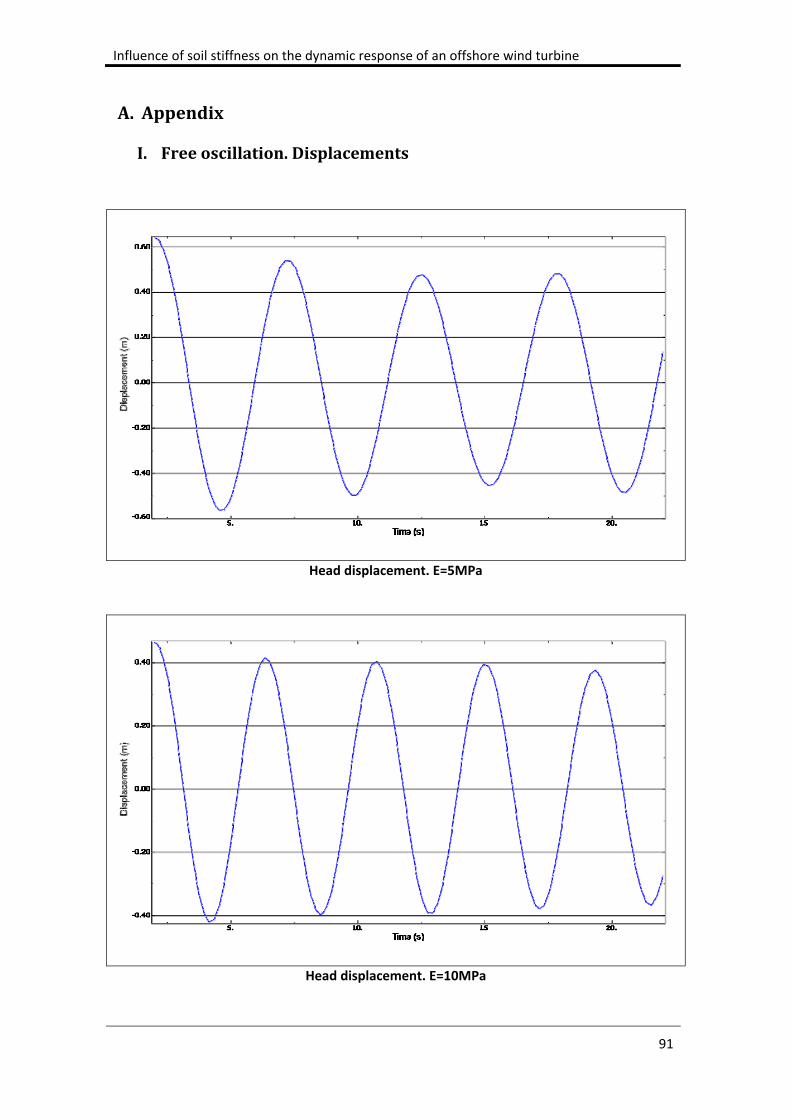
Influence of soil stiffness on the dynamic response of an offshore wind turbine
91
A. Appendix
I. Freeoscillation.Displacements
Head displacement. E=5MPa
Head displacement. E=10MPa
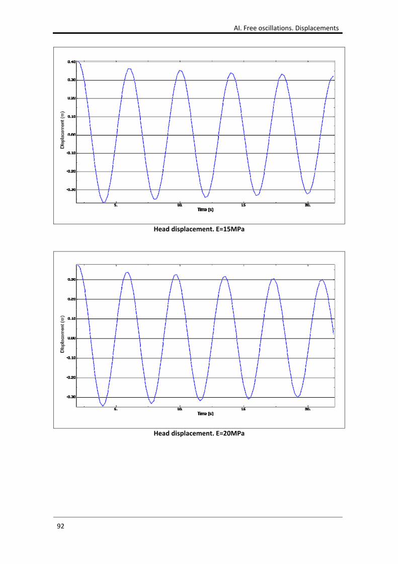
AI. Free oscillations. Displacements
92
Head displacement. E=15MPa
Head displacement. E=20MPa
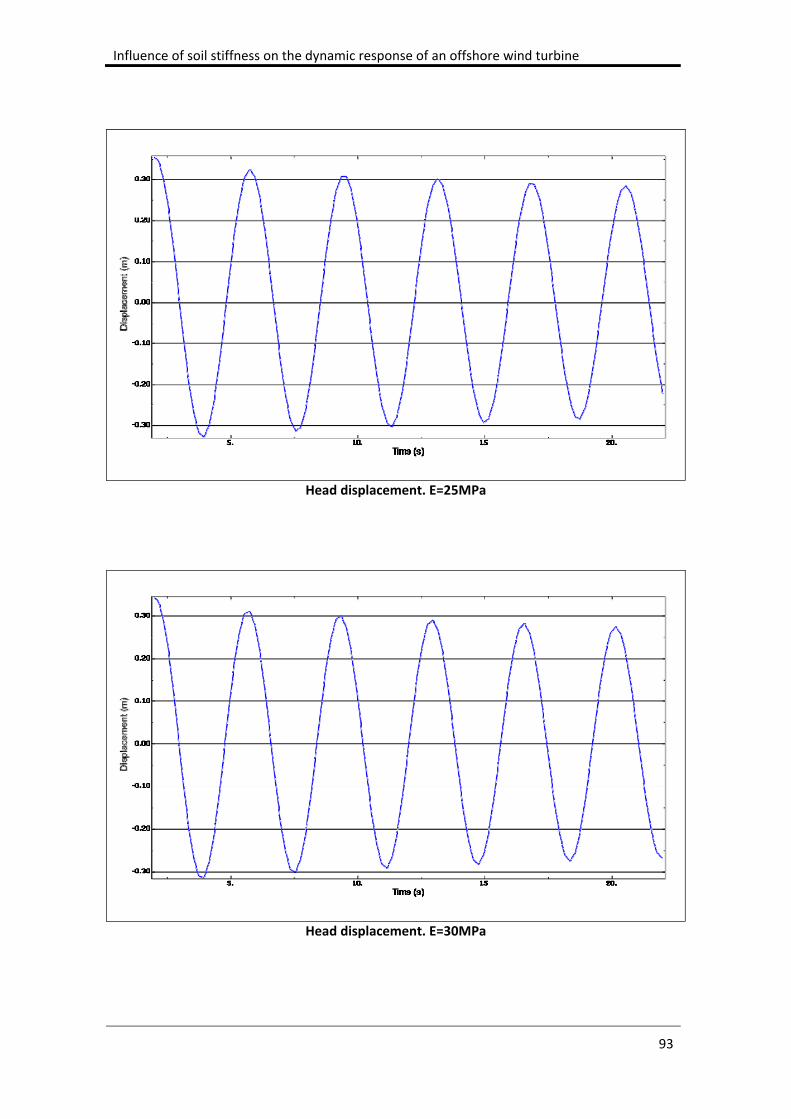
Influence of soil stiffness on the dynamic response of an offshore wind turbine
93
Head displacement. E=25MPa
Head displacement. E=30MPa
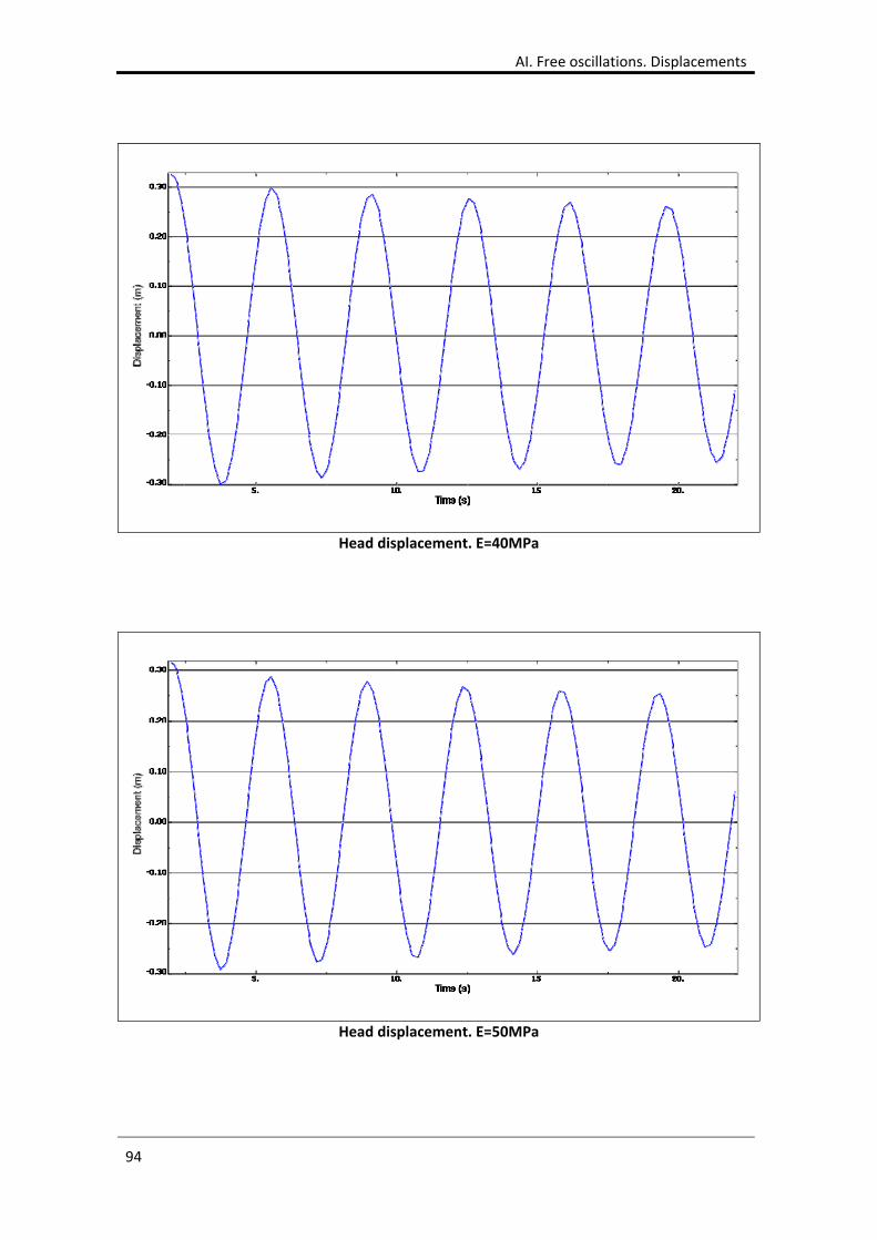
AI. Free oscillations. Displacements
94
Head displacement. E=40MPa
Head displacement. E=50MPa
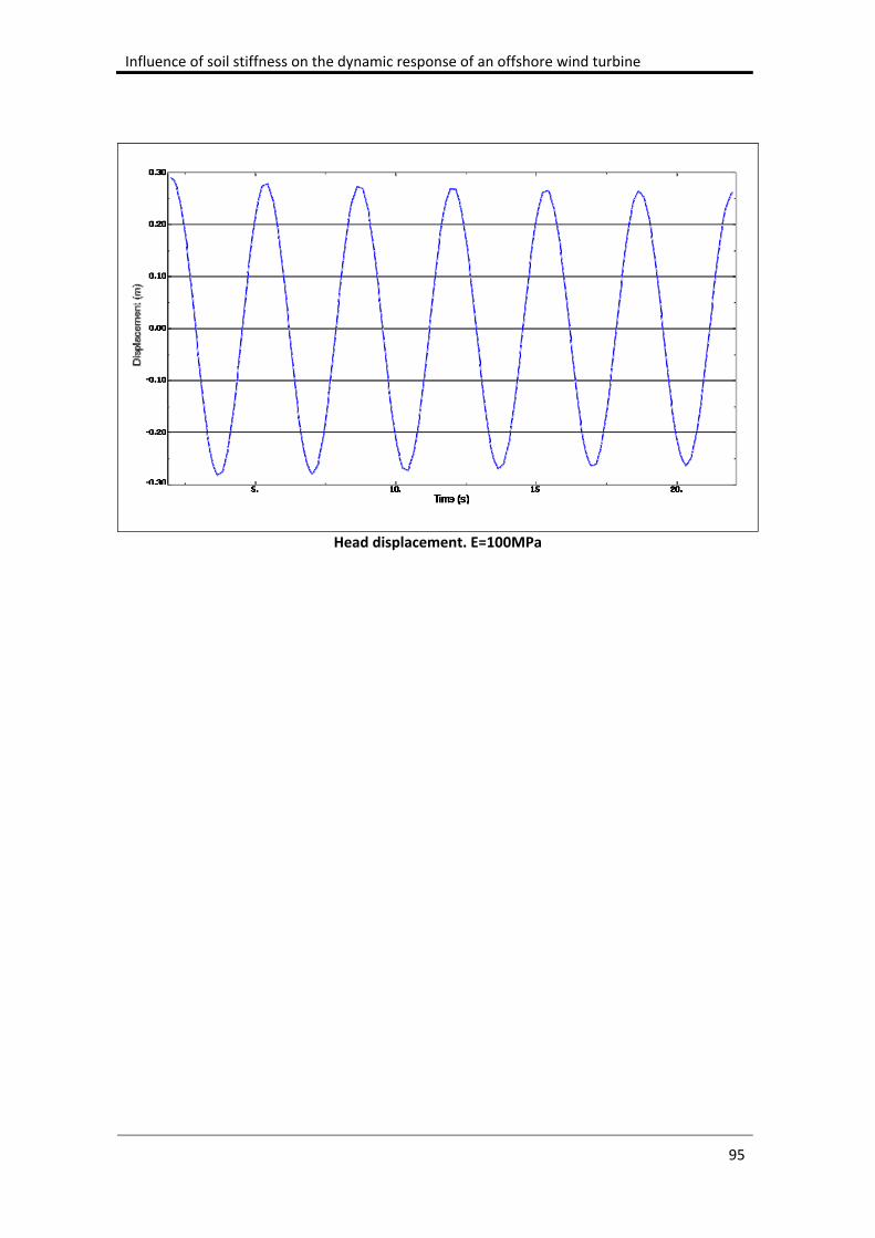
Influence of soil stiffness on the dynamic response of an offshore wind turbine
95
Head displacement. E=100MPa

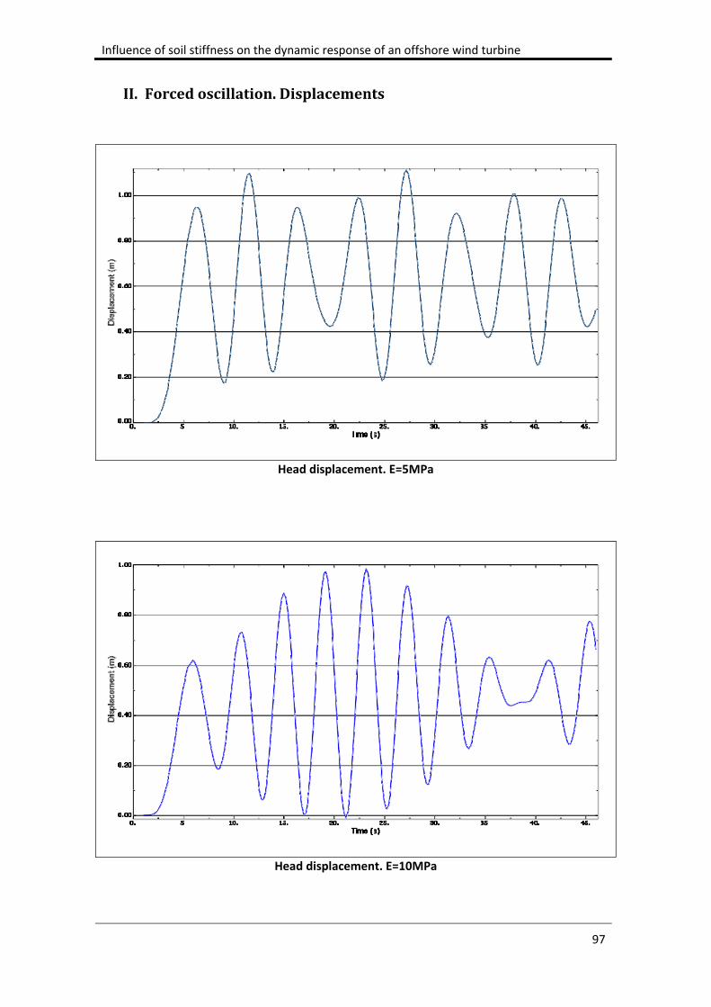
Influence of soil stiffness on the dynamic response of an offshore wind turbine
97
II. Forcedoscillation.Displacements
Head displacement. E=5MPa
Head displacement. E=10MPa
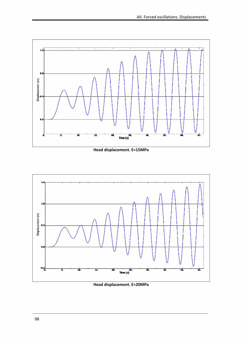
AII. Forced oscillations. Displacements
98
Head displacement. E=15MPa
Head displacement. E=20MPa
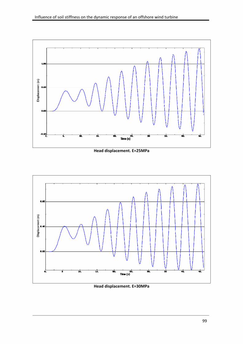
Influence of soil stiffness on the dynamic response of an offshore wind turbine
99
Head displacement. E=25MPa
Head displacement. E=30MPa
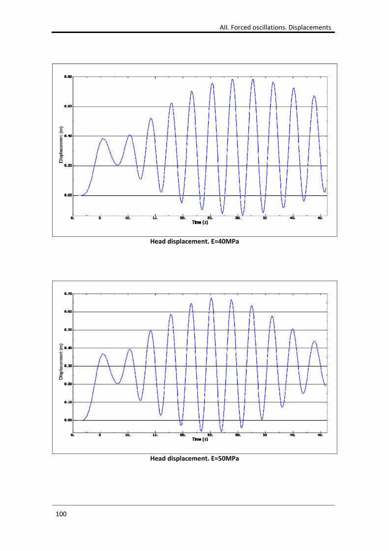
AII. Forced oscillations. Displacements
100
Head displacement. E=40MPa
Head displacement. E=50MPa
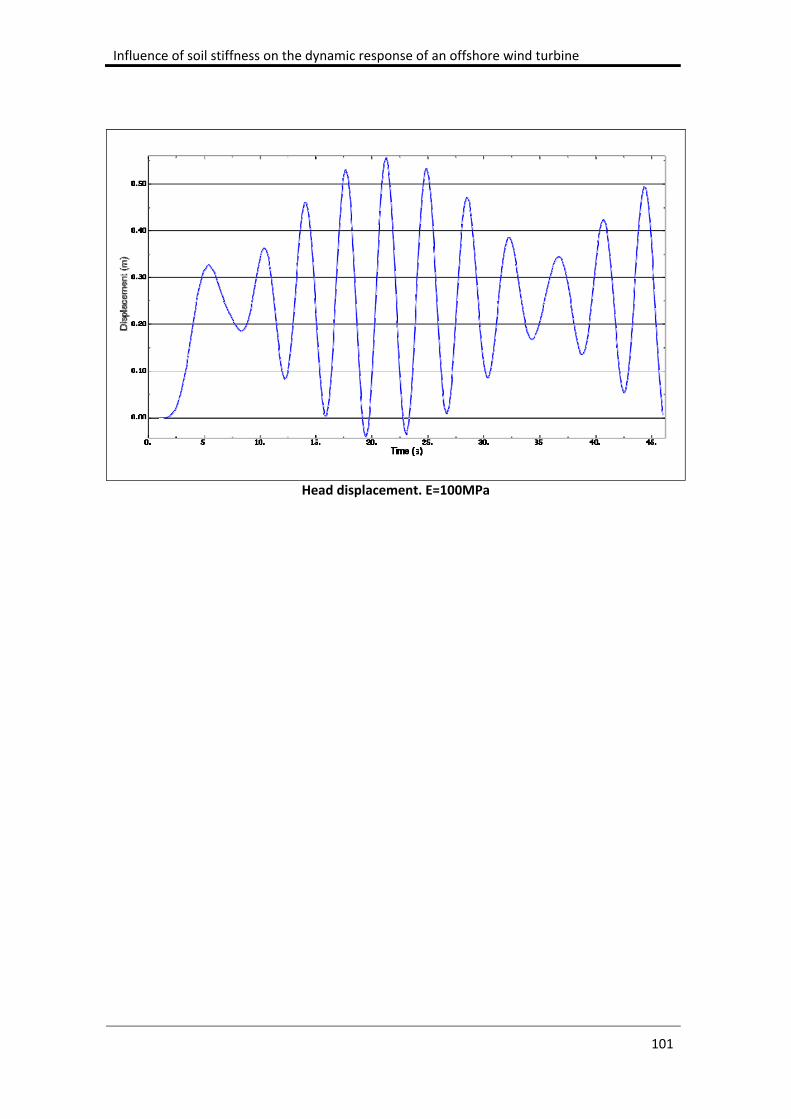
Influence of soil stiffness on the dynamic response of an offshore wind turbine
101
Head displacement. E=100MPa

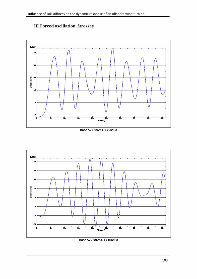
Influence of soil stiffness on the dynamic response of an offshore wind turbine
103
III. Forcedoscillation.Stresses
Base S22 stress. E=5MPa
Base S22 stress. E=10MPa
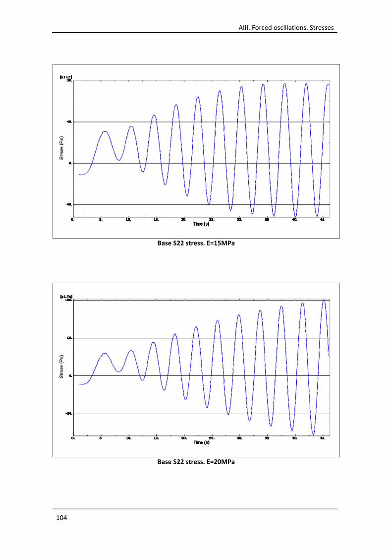
AIII. Forced oscillations. Stresses
104
Base S22 stress. E=15MPa
Base S22 stress. E=20MPa
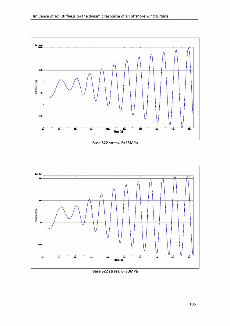
Influence of soil stiffness on the dynamic response of an offshore wind turbine
105
Base S22 stress. E=25MPa
Base S22 stress. E=30MPa
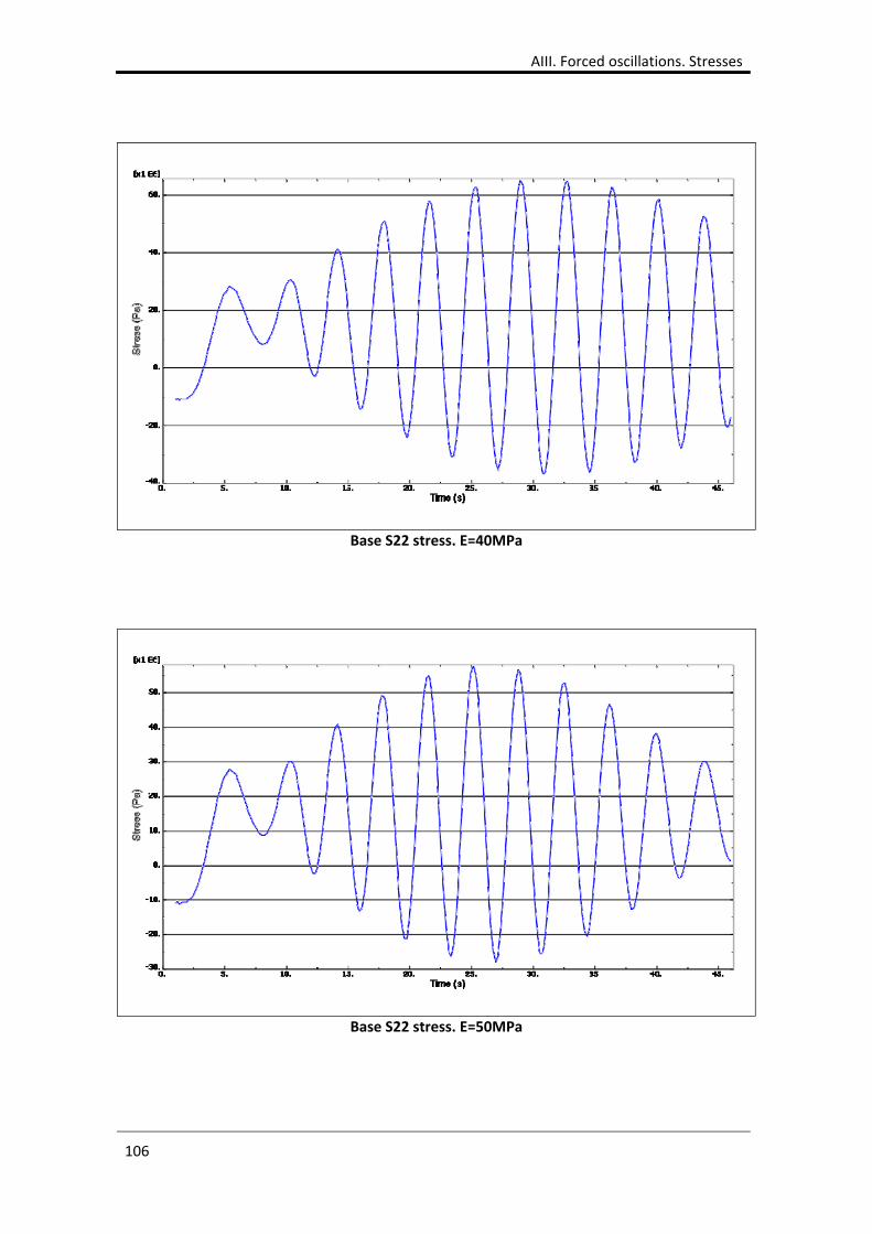
AIII. Forced oscillations. Stresses
106
Base S22 stress. E=40MPa
Base S22 stress. E=50MPa
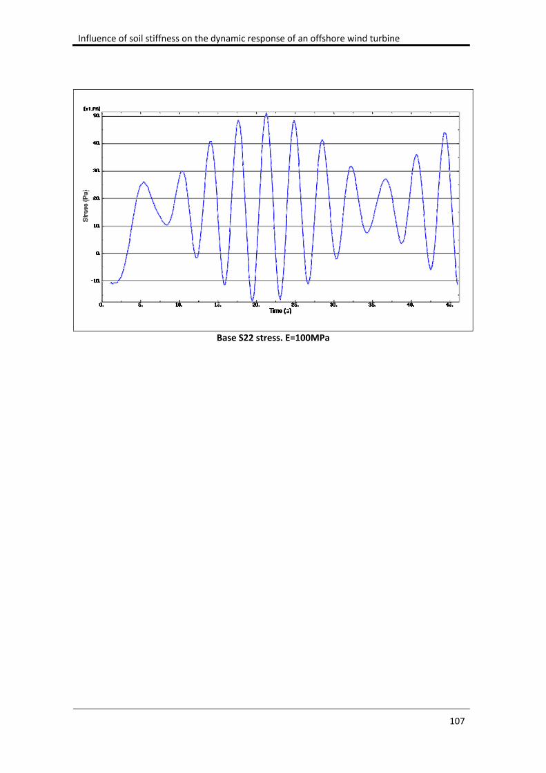
Influence of soil stiffness on the dynamic response of an offshore wind turbine
107
Base S22 stress. E=100MPa

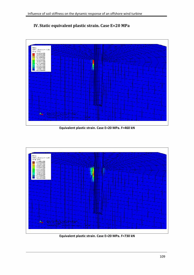
Influence of soil stiffness on the dynamic response of an offshore wind turbine
109
IV. Staticequivalentplasticstrain.CaseE=20MPa
Equivalent plastic strain. Case E=20 MPa. F=460 kN
Equivalent plastic strain. Case E=20 MPa. F=730 kN
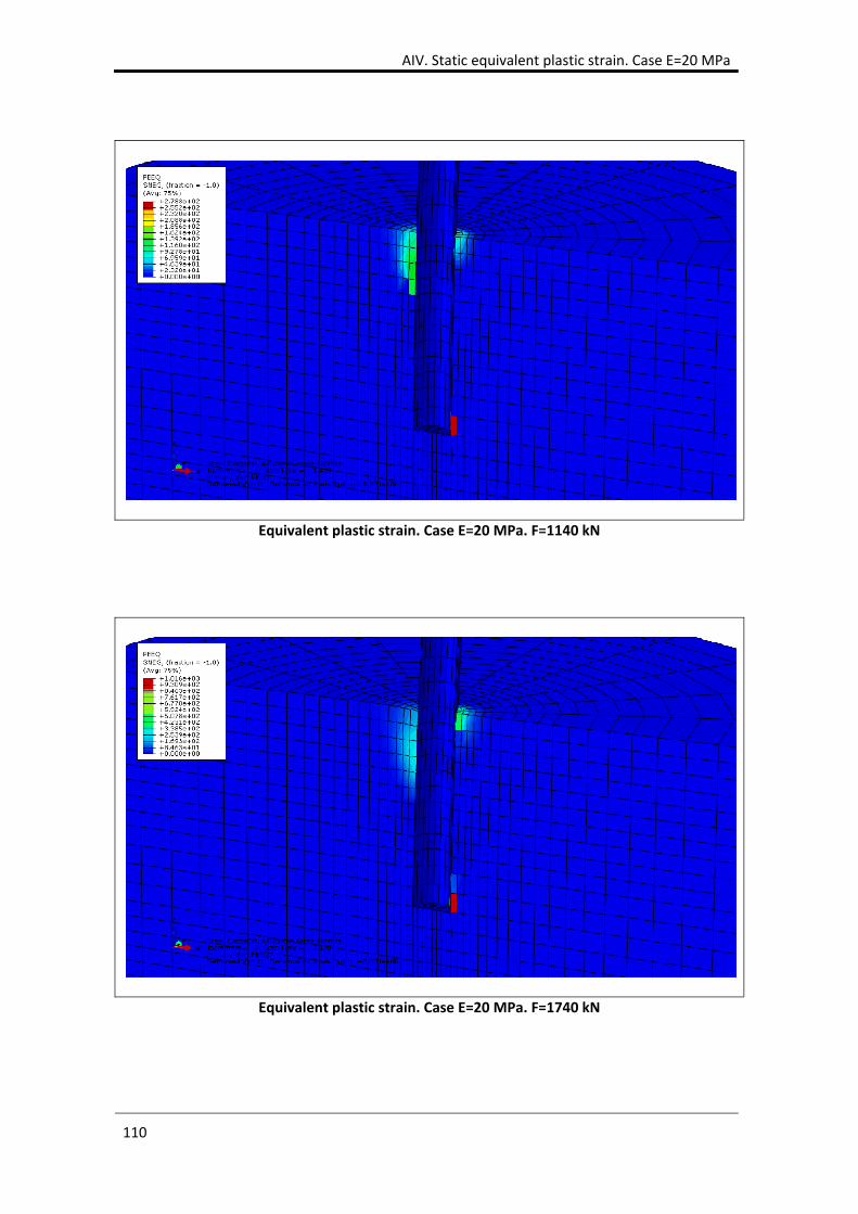
AIV. Static equivalent plastic strain. Case E=20 MPa
110
Equivalent plastic strain. Case E=20 MPa. F=1140 kN
Equivalent plastic strain. Case E=20 MPa. F=1740 kN
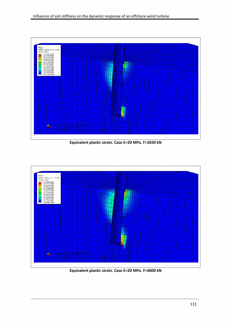
Influence of soil stiffness on the dynamic response of an offshore wind turbine
111
Equivalent plastic strain. Case E=20 MPa. F=2650 kN
Equivalent plastic strain. Case E=20 MPa. F=4000 kN