Mass Action and Concentration Dependence of the Chemical Potential

5. Mass Action and Concentration Dependence of the Chemical Potential

1

5. Mass Action and Concentration Dependence of the Chemical Potential Topic: Concentration dependence of μ and the most important applications. 5.1 The concept of mass action It has been known for a long time that the amounts of reacting substances can play an impor-tant role in the drive of chemical reactions. In 1799, the French chemist Claude-Louis BERTHOLLET was the first to point out this influence and discuss it using many examples. Contrary to the prevailing concept of that time, he stated that a reaction must not necessarily take place fully if a substance B displaces another substance C in a compound,

B + CD → C + BD

(even if there is a great excess of B), but that an equilibrium forms which is dependent upon the amounts of the substances involved. The stronger B is bonded to D, and the greater the amounts of unbound B in the reaction chamber compared to substance C, the more BD should form at the cost of CD and vice versa. Based upon this finding, we can conclude that the tendency μ of substances to change is not only dependent upon the types of those substances, but also upon their amounts n: The greater the amount of a substance (or the mass proportional to it) in the reaction chamber, the higher its expected potential μ should be. Closer scrutiny of this effect which is known as mass ac-tion shows that, in this case, the quantity n itself is unimportant. It is n in relation to the vol-ume V in which a substance is distributed, meaning its concentration c = n/V, that is impor-tant. If B or C, or both, participate as pure substances in a reaction, meaning at fixed concen-trations, their amounts nB and nC have no influence upon the state of equilibrium and there-fore, upon the amounts of BD and CD formed. How much or how little of a substance is pre-sent in this case, is apparently not decisive but rather how densely or loosely it is distributed

in the space. This means that the more cumu-lative and concentrated the application, the more intense the effect. In other words, the mass of a substance is not decisive for mass action, but its “massing”, its “density“ in a space: not the amount, but the concentration. Cato Maximilian GULDBERG and Peter

WAAGE of Norway brought our attention to this in the year 1864. Thus, the chemical potential of substances and the tendency to change increases according to how strongly concentrated they are. Conversely, the chemical potential goes down when the concentration of a substance decreases. We will use an example from everyday life to illus-trate this. According to the values of the chemical potentials, pure water vapour must con-dense at room conditions:


2

H2O|g → H2O|l _______________ μ: −228.6 > −237.1 kG

⇒ A = −8.5 kG However, if the vapour is diluted by air, the value of its potential decreases below that of liquid water. It can then convert to the gaseous state. It evaporates. μ(H2O|g) < μ(H2O|l) is required for wet laundry, wet dishes and wet streets to dry. 5.2 Concentration dependence of chemical potential The influence of concentration c upon the tendency μ of a substance to change can basically be described by a linear relation like it was done in the last chapter to describe the influence of temperature T and pressure p. Δc = c – c0 must be small enough:

0 Δ= + ⋅μ μ γ c for Δc << c. Mass action is an effect which is covered up by other less important influences which will be gone into later on and which all contribute to the concentration coefficient γ : ´ ´́ ...γ γ γ γ×

= + + + . The symbol × above a term will be used here and in the following to denote the quantities de-pendent upon mass action when these should be distinguished from similar quantities with other origins. Mass action appears most noticeably at small concentrations where the other influences recede more and more until they can be totally neglected, ,́ ´́ , ...γ γ γ×

>> . If one wishes to investigate this effect most easily, experiments can be done with strongly diluted solutions c << c ( = 1 kmol⋅m−3). The temperature coefficient α and the pressure coefficient β (except the latter in the case of gases) are not only different from substance to substance but also vary according to type of solvent, temperature, pressure, concentration, etc. In short, they depend upon the entire com-position of the milieu they are in. In contrast, the concentration coefficient γ× related to mass action is a universal quantity. At the same T and c, it is the same for all substances in every milieu. It is directly proportional to the absolute temperature T and inversely proportional to concentration c of the substance in question and has the same basic structure as the pressure coefficient β of gases:

RTγ γc

×= ≡ for c << c where R = 8.314 G⋅K−1.

Because the quantity T is in the numerator, we can conclude that the mass action gradually loses importance with a decrease of temperature and eventually disappears at 0 K. If we insert the second equation into the first one, we obtain the following relation

0 ΔRTμ μ cc

= + ⋅ for Δc << c << c. Analogous to the treatment of the pressure coefficient β of gases, a logarithmic relation be-tween μ and c results:


3

⎟⎟⎠

⎞⎜⎜⎝

⎛+=

00 ln

ccRTμμ for c, c0 << c (mass action equation 1).

We will return to the term „mass action equation“ below. As already mentioned, precise measurements show that the relation above is not strictly ad-hered to. At higher concentrations, values depart quite noticeably from this relation. If we gradually move to lower concentrations, the differences become smaller. The equation here expresses a so-called “limiting law“ which strictly applies only when c → 0. For this reason, we have added the requirement for a small concentration (c, c0 << c) to the equation. In practice, this relation serves as a useful approximation up to rather high concentrations. In the case of electrically neutral substances, deviations are only noticeable above 100 mol⋅m−3. For ions, deviations become observable above 1 mol⋅m−3, but they are so small that they are easily neglected if accuracy is not of prime concern. For practical applications let us remem-ber that:

⎟⎟⎠

⎞⎜⎜⎝

⎛+≈

00 ln

ccRTμμ for c <

However, it is precisely for standard concentration c = 1000 mol⋅m−3 = 1 mol⋅L−1 (the usual reference value), where the logarithmic relation is not satisfied for any substance. Still, this concentration is used as the usual starting value for calculating potentials, and we write:

rln lncμ μ RT μ RT cc

⎛ ⎞= + = +⎜ ⎟⎝ ⎠

○ ○

for c << c (mass action equation 1´).

Here, cr is the relative concentration. The μ○ , intended as the basic value (at fixed concentra-tion c) has been chosen so that the equation gives the right results at low values of concen-tration. In contrast to the mass action equation 1, the initial value of μ is no longer real, but fictive. Note that the basic value μ of a dissolved substance B depends upon pressure p and temperature T, Bμ

○ (p, T). This distinguishes it from the standard value Bμ ≡ Bμ

○ (p, T) al-ready known to us. The term RTlncr = μ× is also called the mass action term. In its first or second version, this law describes mass action formally as a characteristic of the chemical potential. We give these equations a name in order to refer to them more easily. In fact, we will give all relations of this type (there are several more of them) the same name, „mass action equations.” As expected, the tendency of a substance to change increases with its concentration. This does not happen linearly, though, but logarithmically. We obtain the following graph for the dependence of the chemical potential of a dissolved substance upon its concentration:

100 mol⋅m−3 for neutral substances, 1 mol⋅m−3 for ions.


4

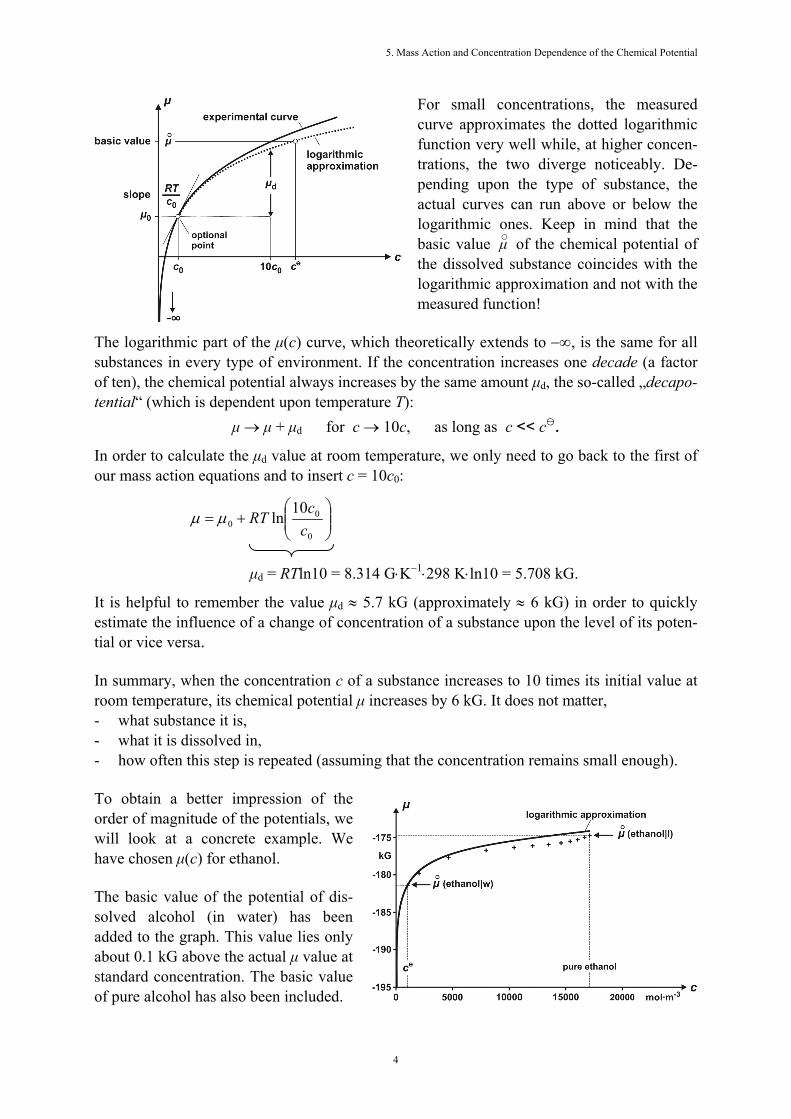
For small concentrations, the measured curve approximates the dotted logarithmic function very well while, at higher concen-trations, the two diverge noticeably. De-pending upon the type of substance, the actual curves can run above or below the logarithmic ones. Keep in mind that the basic value μ○ of the chemical potential of the dissolved substance coincides with the logarithmic approximation and not with the measured function!

The logarithmic part of the μ(c) curve, which theoretically extends to −∞, is the same for all substances in every type of environment. If the concentration increases one decade (a factor of ten), the chemical potential always increases by the same amount μd, the so-called „decapo-tential“ (which is dependent upon temperature T):

μ → μ + μd for c → 10c, as long as c << c. In order to calculate the μd value at room temperature, we only need to go back to the first of our mass action equations and to insert c = 10c0:

⎟⎟⎠

⎞⎜⎜⎝

⎛+=

0

00

10lnccRTμμ

μd = RTln10 = 8.314 G⋅K−1⋅298 K⋅ln10 = 5.708 kG. It is helpful to remember the value μd ≈ 5.7 kG (approximately ≈ 6 kG) in order to quickly estimate the influence of a change of concentration of a substance upon the level of its poten-tial or vice versa. In summary, when the concentration c of a substance increases to 10 times its initial value at room temperature, its chemical potential μ increases by 6 kG. It does not matter, - what substance it is, - what it is dissolved in, - how often this step is repeated (assuming that the concentration remains small enough). To obtain a better impression of the order of magnitude of the potentials, we will look at a concrete example. We have chosen μ(c) for ethanol. The basic value of the potential of dis-solved alcohol (in water) has been added to the graph. This value lies only about 0.1 kG above the actual μ value at standard concentration. The basic value of pure alcohol has also been included.


5

Using the newly extracted relations, we will again take a closer look at evaporation. When the vapour is diluted by air, say, by a factor of 100 (by two orders of magnitude), its potential goes down by around 2⋅5.7 kG = 11.4 kG to about −240.0 kG. At that point, μ(H2O|g) actually lies below the value for liquid water and evaporation takes place. At a concentration of 1

30 , the air is already so moist that it cannot absorb any more water. It is said to be saturated. A concentration of 1

30 means about 1.5 orders of magnitude below the concentration of pure vapour. Therefore, the water vapour potential lies about 1.5⋅5.7 kG = 8.6 kG below the value for pure vapour. At –237.2 kG, it is at about the same level as that of liquid water and the drive to evaporate disappears. Even a little higher concentration leads to condensation and the excess water precipitates as dew. 5.3 Concentration dependence of chemical drive We can now use what we have learned to easily show how shifts of concentration effect the chemical drive to react. Observe the following reaction

B + C + … → D + E + …

between dissolved substances, meaning a homogeneous reaction. The drive results in

[ ] [ ]B C D E... ...μ μ μ μ= + + − + +A .

If all the substances are present in small concentrations, we can apply the mass action equati-on for all of them:

r r r rB C D Eln (B) ln (C) ... ln (D) ln (E) ...μ RT c μ RT c μ RT c μ RT c⎡ ⎤ ⎡ ⎤= + + + + − + + + +⎢ ⎥ ⎢ ⎥⎣ ⎦ ⎣ ⎦○ ○ ○ ○

A .

The terms of the equation can be sorted a bit

[ ]r r r rB C D E... ... ln (B) ln (C) ... ln (D) ln (E) ...μ μ μ μ RT c c c c⎡ ⎤= + + − − − + + + − − −⎢ ⎥⎣ ⎦○ ○ ○ ○

A and the final result is

r r

r r

(B) (C) ...ln(D) (E) ...

c cRTc c

⋅ ⋅= +

⋅ ⋅A A

○ .

We have A

○ = (B) (C) ... (D) (E) ...μ μ μ μ+ + − − −

○ ○ ○ ○ for the basic term A○

. It expresses the drive when all reaction partners have the standard concentration of 1000 mol⋅m−3.

...)E()D(

...)C()B(lnrr

rr

⋅⋅⋅⋅

ccccRT = ×

A in turn, represents the mass action term.

We will explain the influence of concentration shifts upon the drive using the example of de-composing cane sugar

Suc|w + H2O|l → Glc|w + Fru|w

Suc is the abbreviation for cane sugar (sucrose, C12H22O11), Glc and Fru represent the iso-meric monosaccharides grape sugar (glucose, C6H12O6) and fruit sugar (fructose, C6H12O6). From the chemical potentials, we obtain the following for the drive A:


6

2Suc H O Glc Fru= + − −μ μ μ μA

2

Suc Glu FruSuc H O Glc Fruln ln lnc c cμ RT μ μ RT μ RT

c c c⎛ ⎞ ⎛ ⎞ ⎛ ⎞= + + − − − −⎜ ⎟ ⎜ ⎟ ⎜ ⎟⎝ ⎠ ⎝ ⎠ ⎝ ⎠

○ ○ ○ ○

2

SucSuc H O Glu Fru

Glc Fru

ln c cμ μ μ μ RTc c

⎛ ⎞⋅= + − − + ⎜ ⎟⋅⎝ ⎠

○ ○ ○ ○ .

A○

In this mathematical description, we cannot apply the mass action equation to water because its concentration lies far outside the equation’s range of validity, cH2O ≈ 50000 mol⋅m−3. The potential curves for high c values are very flat, and the cH2O value in dilute solutions does not differ significantly from the concentration for pure water so it is possible to replace the actual

OH2μ value with that of pure water. We will indicate the potential for the pure solvent (in this case water) similarly to the basic potentials of dissolved substances μ○ :

2H Oμ○ . In general, sol-vents of dilute solutions can be approximated well by pure substances. A brief comment about how to write arguments and indexes: μ(H2O), c(H2O) ... and OH2

μ , OH2

c ... are treated as equivalent forms. In the case of long names of substances or substance formulas with indexes (such as H2O) or an accumulation of indexes, the preferred way of writing is the first one, otherwise, for the sake of brevity, the second. For the more general reaction

...ED...CB EDCB ++→++ νννν we correspondingly obtain

[ ]B B C C D D E E... ...ν μ ν μ ν μ ν μ= ⎡ + + ⎤ − + +⎣ ⎦A .

If the concentration dependence of the chemical potential is taken into account, it results in

B B r C C rB ln (B) ln (C) ...Cν μ ν RT c ν μ ν RT c⎡ ⎤= + + + +⎢ ⎥⎣ ⎦○ ○

A

D D r E E rD Eln (D) ln (E) ...ν μ ν RT c ν μ ν RT c⎡ ⎤− + + + +⎢ ⎥⎣ ⎦○ ○ .

We can rearrange

B C D EB C D E... ...ν μ ν μ ν μ ν μ⎡ ⎤+ + − − −⎢ ⎥⎣ ⎦○ ○ ○ ○

A =

B r C r D r E rln (B) ln (C) ... ln (D) ln (E) ...RT ν c ν c ν c ν c+ ⎡ + + − − − ⎤⎣ ⎦ and obtain

CB

D E

r r

r

(B) (C) ...ln(D) (E) ...

νν

ν νr

c cRTc c

⋅ ⋅= +

⋅ ⋅○

A A .


7

Let us now take another look at a concrete example. For this, we choose the reaction of Fe3+ ions with I− ions:

2 Fe3+|w + 2 I−|w → 2 Fe2+|w + I2|w. Therefore, the conversion numbers are: 3+Fe

ν = −2, -Iν = −2, 2+Fe

ν = +2 und 2Iν = +1. Insertion

into the formula above results in:

3+ 2 - 2r r

2+ 2r r 2

(Fe ) (I )ln(Fe ) (I )

c cRTc c

⋅= +

⋅○

A A .

However, the concentrations do not remain constant during a reaction. They change in the process of the reaction. If there is only one substance at the beginning, its concentration de-creases continuously to the benefit of the product. Using the simplest reaction possible, we will discuss the conversion of a substance B into a substance D:

B D.→

An example would be the transformation of α-D-glucose into the isomeric β-D-glucose in aqueous solution. These two stereoisomers of glucose C6H12O6, differ only in the placement of the OH group relative to the chiral center (characterised by *) formed by the ring closure.

α-D-Glucose|w β-D-Glucose|w→ (The transformation takes place via the open-chain form, but its concentration is so small that it can be ignored.) The two substances are optically active: pure α-D-glucose shows an angle of rotation of +112°, pure β-D-glucose, however, one of +18,7°. Therefore, a polarimeter can be used to observe the change in the solution’s angle of rotation. When crystals of pure α-D-glucose are dissolved in water, the specific rotation of the solution decreases gradually from an initial value of +112° to a value of +53°. In section 1.6, the extent of reaction ξ was introduced as a measure of the progress of a reac-tion. It was defined by

0Δ ( ) ( )i i i

i i

n n t n tξν ν

−= = .

The extent of reaction can now be easily converted to the time dependent change of concen-tration, and respectively, to the concentration at time t:

00

( ) ( )Δ ( ) ( ) −= − = =i i i

i i in t n t ν ξc c t c t

V V

or rather


8

0( ) ( ) ii i

ν ξc t c tV

= + .

The drive of a reaction changes along with the concentrations. If one assumes a concentration of c0 of the initial substance as well as an absence of the product at the beginning of the reac-tion at t0 = 0, the following relation for the dependence of the drive upon the extent of reac-tion is obtained:

0 0( / ) / /ln ln( / ) / /

c ξ V c c ξ VRT RTξ V c ξ V− −

= + = +○ ○

A A A

.

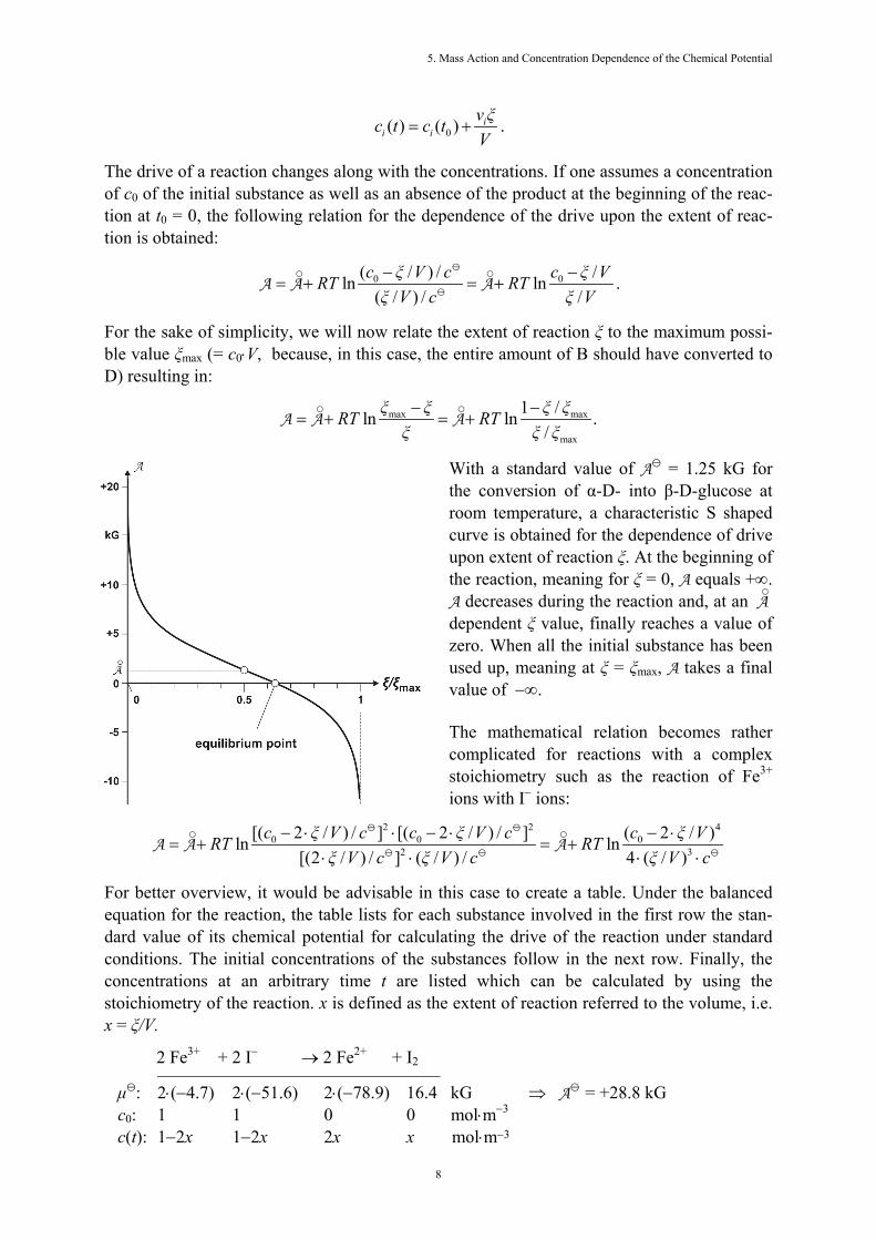
For the sake of simplicity, we will now relate the extent of reaction ξ to the maximum possi-ble value ξmax (= c0⋅V, because, in this case, the entire amount of B should have converted to D) resulting in:

max max

max

1 /ln ln ./

ξ ξ ξ ξRT RTξ ξ ξ

− −= + = +

○ ○A A A

With a standard value of A = 1.25 kG for the conversion of α-D- into β-D-glucose at room temperature, a characteristic S shaped curve is obtained for the dependence of drive upon extent of reaction ξ. At the beginning of the reaction, meaning for ξ = 0, A equals +∞. A decreases during the reaction and, at an A

○

dependent ξ value, finally reaches a value of zero. When all the initial substance has been used up, meaning at ξ = ξmax, A takes a final value of −∞. The mathematical relation becomes rather complicated for reactions with a complex stoichiometry such as the reaction of Fe3+ ions with I− ions:

2 2 4

0 0 02 3

[( 2 / ) / ] [( 2 / ) / ] ( 2 / )ln ln[(2 / ) / ] ( / ) / 4 ( / )

c ξ V c c ξ V c c ξ VRT RTξ V c ξ V c ξ V c

− ⋅ ⋅ − ⋅ − ⋅= + = +

⋅ ⋅ ⋅ ⋅○ ○

A A A

For better overview, it would be advisable in this case to create a table. Under the balanced equation for the reaction, the table lists for each substance involved in the first row the stan-dard value of its chemical potential for calculating the drive of the reaction under standard conditions. The initial concentrations of the substances follow in the next row. Finally, the concentrations at an arbitrary time t are listed which can be calculated by using the stoichiometry of the reaction. x is defined as the extent of reaction referred to the volume, i.e. x = ξ/V.

2 Fe3+ + 2 I− → 2 Fe2+ + I2 ________________________________ μ: 2⋅(−4.7) 2⋅(−51.6) 2⋅(−78.9) 16.4 kG ⇒ A = +28.8 kG c0: 1 1 0 0 mol⋅m−3 c(t): 1−2x 1−2x 2x x mol⋅m−3


9

Again, we obtain the typical S shaped curve. Let us remind ourselves about the criteria for a reaction which we were introduced to in Chapter 3: A reaction takes place voluntarily as long as drive A is positive. At A = 0, there is equilibrium. A negative drive forces a reaction backwards against the direction the reaction arrow points in. Here are some important consequences for the reaction process: - Every homogeneous reaction begins voluntarily. - At a certain extent of reaction, it stops in

equilibrium with the environment. - Equilibrium can be reached from both sides, meaning from the side with the initial sub-

stances as well as from the side with the reaction products. In equilibrium, neither the forward reaction nor the backward reaction take place voluntarily. Macroscopically speaking, there is no more conversion and the composition of the reaction mixture remains constant. However, forward and backward reactions do continue to occur at the microscopic level between the particles. These happen at identical rates though, so that the conversions in the two directions compensate for each other. In this case, one speaks of a dy-namic equilibrium. 5.4 The mass action law What is commonly known as the mass action law as defined by GULDBERG and WAAGE, is a consequence of a combination of the mass actions of individual substances participating in a reaction. Let us, once again, consider a reaction in a homogenous solution

B + C + … D + E + … . Equilibrium rules when there is no longer any potential drop and the drive A disappears. The-refore:

r r

r r

(B) (C) ...ln 0(D) (E) ...

c cRTc c

⋅ ⋅= + =

⋅ ⋅A A

○.

When we divide by RT and take the antilogarithm, we obtain

r r

r r

(D) (E) ...(B) (C) ... eq.

cc cc c

⎛ ⎞⋅ ⋅= ⎜ ⎟⋅ ⋅⎝ ⎠

○K with : expc RT

⎛ ⎞⎜ ⎟=⎜ ⎟⎝ ⎠

A○

○K .

This equation characterizes the relationship between concentrations in equilibrium which has been referred to by the index eq. and shows a possible form of the mass action law for the


10

reaction. The quantity c○

K which is called the equilibrium constant of the reaction is so named because it does not depend upon the concentration of the substances. A more precise name, however, would be equilibrium number because c

○K is a number and it is not constant but

dependent upon temperature, pressure, solvent, etc. The index ○ which is actually superflu-ous, has been inserted in order to emphasize that

○K is to be formed from A

○ (and not from

A!). For the more general reaction

B C D EB C ... D E ...ν ν ν ν+ + + + we obtain entirely appropriately

D E

CB

r r

r r

(D) (E) ...(B) (C) ... eq.

ν ν

c νν

c cc c

⎛ ⎞⋅ ⋅= ⎜ ⎟⎜ ⎟⋅ ⋅⎝ ⎠

○K .

Commonly, the relative concentrations cr are replaced by c/c and the fixed standard concen-tration c is combined with the equilibrium number c

○K to form the new equilibrium constant

cK○

(κ „dimension factor“):

c cK κ=○ ○

K , where κ = (c) cν with νc = νB + νC + ... + νD + νE + ... .

νc is the sum of all conversion numbers which, in our example, are −1 for the initial sub-stances B, C, ... and +1 for the products D, E, ... . As stated above, c

○K is always a number

while the constant cK○

has the unit (mol⋅m−3) cν . Only when νc happens to be 0, are cK○

and cK

○ identical. cK

○ is the more convenient quantity for formulating the mass action law,

D E

B C

...

... eq.c

c cKc c

⎛ ⎞⋅ ⋅= ⎜ ⎟⋅ ⋅⎝ ⎠

○,

while, for general considerations, c○

K is preferred since its dimension is the same for all reac-tions. Here is an example of what has been said. With the help of a table, we will determine the acidity constant of acetic acid (CH3COOH), abbreviated to HAc, in an aqueous solution, i.e., the equilibrium constant for the dissociation

HAc|w H |w Ac |w+ −+

or the equilibrium constant for the proton exchange in BRØNSTED’s sense (this will be dis-cussed more detailed in the next chapter):

2 3HAc|w H O|l H O |w Ac |w+ −+ + .

The formulas are two different versions of the same process. In the first case, the mass action law is written as

r r,1

r

(H ) (Ac )(HAc)c

c cc

+ −⋅=

○K

where


11

-HAc H Ac,1 exp expc

μ μ μRT RT

+⎛ ⎞⎛ ⎞ − −⎜ ⎟⎜ ⎟= =⎜ ⎟⎜ ⎟

⎝ ⎠ ⎝ ⎠

A○ ○ ○ ○

○K

3

1

( 396.46 0 369.31) 10 Gexp8.314 G K 298 K−

⎛ ⎞− − + ⋅= =⎜ ⎟⋅ ⋅⎝ ⎠

1.74⋅10−5

and in the usual way as

,1(H ) (Ac )

(HAc)c

c cKc

+ −⋅=

○

where

5 3,1 ,1 1.74 10 kmol mc cK c − −= ⋅ = ⋅ ⋅

○ ○K

with νc = −1 + 1 + 1 = +1 and therefore the dimension factor κ = c = 1 kmol⋅m−3. In the second case, when we take into account that the solvent water can be treated as a pure substance, we obtain for the mass action law:

r 3 r,2

r

(H O ) (Ac )(HAc)c

c cc

+ −⋅=

○K

where

2 3,2

(HAc) (H O) (H O ) (Ac )expcμ μ μ μ

RT

+ −⎛ ⎞+ − −⎜ ⎟= ⎜ ⎟⎝ ⎠

○ ○ ○ ○○

K

3

1

( 396.46 237.14 237.14 369.31) 10 Gexp8.314 G K 298 K−

⎛ ⎞− − + + ⋅= =⎜ ⎟⋅ ⋅⎝ ⎠

1.74⋅10−5

and written in the usual way,

3,2

(H O ) (Ac )(HAc)

cc cK

c

+ −⋅=

○

where

5 3,2 ,2 1.74 10 kmol mc cK c − −= ⋅ = ⋅ ⋅

○ ○K .

Also in this case the dimension factor results in κ = c = 1 kmol⋅m−3, because the solvent wa-ter is treated as pure substance and therefore does not appear in the sum νc of conversion num-bers . The equilibrium constants ,1c

○K and ,2c

○K (or ,1cK

○ and ,2cK

○) have the same value. The same

acidity constant S○

K = ,1c○

K = ,2c○

K is obtained independent of whether the first or second reac-tion equation is applied, meaning whether the process is considered as dissociation or proton exchange. The mass action law’s range of validity is the same as that of the mass action equations (from which it is derived). The smaller the concentrations, the more strictly the law applies. At higher concentrations, deviations occur as the result of ionic or molecular interactions.


12

The magnitude of the equilibrium number determined according to

lnRT=○ ○

A K

is a good qualitative indication for how a reaction proceeds. The more strongly positive ○

A is, the greater

○K ( 1>>

○K ) is. In this case, the end products dominates in the equilibrium compo-

sition. Because of the logarithmic relation, even small changes to ○

A lead to noticeable shifts in the equilibrium point. On the other hand, if

○A is strongly negative,

○K approaches zero

( 1<<○

K ) and the initial substances dominate in the composition of the equilibrium. At the same time, this also means that, even for negative

○A , a small amount of the initial substance

is still converted to the end products because ○

K has a small yet finite value. When ○

A ≈ 0 and therefore

○K ≈ 1, the initial substances and end products are present in comparable amounts in

equilibrium. (Keep in mind, however, that in all three cases discussed, A = 0! since we have equilibrium.) With the help of the equilibrium number or the conventional equilibrium constant, the equilib-rium composition of a mixture which has formed by voluntary conversion of given amounts of initial substances can be quantitatively determined. If, for example, pure α-D-glucose at the concentration 0.1 mol/L is dissolved in water, one can use a polarimeter to observe a continu-ous change to the angle of rotation until a constant value is finally achieved. This can be as-cribed to the partial conversion of α-D-glucose into β-D-glucose (remember the discussion further above). If we indicate the concentration of β-D-glucose in equilibrium by x, we obtain

0

expeq.

cxK

RT c x

⎛ ⎞ ⎛ ⎞⎜ ⎟= = ⎜ ⎟⎜ ⎟ −⎝ ⎠⎝ ⎠

○○ A .

The dimension factor κ equals 1 because of νc = 0. The equilibrium constant at room tempera-ture can be calculated by use of the standard value A = 1.25 kG (see section 5.3):

3

31

1, 25 10 Gexp 1,66 kmol m8,314 G K 298 K

−−

⎛ ⎞⋅= = ⋅⎜ ⎟⋅ ⋅⎝ ⎠

○cK

From now on, we will not use the rather cumbersome index eq. as long as it is clear from the relation, as in this example, that we are dealing with the equilibrium composition. Solving for x results in:

0 1.66 0.1mol/L 0.0624 mol/l1.66 11

⋅ ⋅= = =

++

○

○

c

c

K cxK

.

According to this, the state of equilibrium shows that 37.6 % of all dissolved molecules are α-D-glucose molecules and 62.4 % are β-D-glucose molecules. The mathematical relations become rather complicated for reactions with a more complex stoichiometry. If we like to determine for example the equilibrium composition in the case of the reaction

2 Fe3+|w + 2 I−|w → 2 Fe2+|w + I2|w

characterised by the table above, we obtain


13

3

4

4exp(1 2 ) eq.

cxK κ

RT x

⎛ ⎞ ⎛ ⎞⎜ ⎟= ⋅ = ⎜ ⎟⎜ ⎟ −⎝ ⎠⎝ ⎠

○○ A

with the dimension factor 1( )κ c −= = 1 kmol−1⋅m3 (because of νc = −2 − 2 + 2 + 1 = −1). Because the value of

○A is positive and relatively high (

○A = +29 kG), we have 1c

○K , i.e.

we can expect that the end products dominate in the equilibrium composition. For more de-tailed data we have to solve for x the equation above. Because a higher degree polynomial is involved a numerical technique using an appropriate mathematical software or a graphical approach are advisable. An equilibrium point of ξ/ξmax ≈ 0.79 can be obtained from the figure in section 5.3. The concentrations of the substances in the equilibrium mixture are therefore c(Fe3+) ≈ 0.21 mol⋅m−3 und c(I−) ≈ 0.21 mol⋅m−3 for the initial substances and c(Fe2+) ≈ 0.79 mol⋅m−3 und c(I2) ≈ 0.39 mol⋅m−3 for the final products, respectively. The equation above can be reversely used to experimentally determine the basic drive

○A of a

reaction. In order to do this, it is enough to first calculate the constant ○

K and then to derive○

A from it. At first glance, this looks amazingly easy, but the reaction can be so strongly inhibited that the concentrations being determined do not correspond to equilibrium values. This obsta-cle can be overcome, though, by adding a catalyst. As long as the added amount is small the position of equilibrium does not change and we can directly use the equlilibrium values ob-tained in the equation above. When the basic drive is known the drive for any other concentra-tions can be calculated provided that the c values are small (c << c). 5.5 Special versions of the mass action equation Until now, we have described mass action by using functions in which the concentrations c or, more exactly, the ratios c/c0 or c/c appear as arguments. Instead of c, it would be possible to introduce any other measure of composition as long as it is proportional to concentration. This is almost always the case at small c values. We will highlight two of these measures here be-cause they are of greater importance. When the pressure on a gas is increased, the concentration of the gas particles also increases because they are compressed into a smaller volume. If the temperature remains unchanged, the concentration grows proportionally to the pressure: c ~ p, or

00 pp

cc

= .

As a result, the concentration ratio in the mass action equation for gases can be replaced by the pressure ratio:

⎟⎟⎠

⎞⎜⎜⎝

⎛+=

00 ln

ppRTμμ für p, p0 << 10 p (mass action equation 2).

This equation is precise enough to be applied to pressures up to about 102 kPa (1 bar). It also lends itself to estimates up to 103 or even 104 kPa. In anticipation of this, we have applied the


14

equation above to treating the pressure dependence of the chemical potential of gases (section 4.5). The mass action equation 2 can be generalized somewhat. In the case of gaseous mixtures, one imagines that each component B, C, D, ... produces a partial pressure which is independ-ent of its partners in the mixture. This corresponds to the pressure that the gaseous compo-nents would have if they alone were to fill up the available volume. The total pressure p of the gaseous mixture is simply equal to the sum of the partial pressures of all the components pre-sent (DALTON’s law):

p = pB + pC + pD + ... (as well as c = cB + cC + cD + ...). If a gas is compressed, the concentrations of all the components and the partial pressures in-crease. This is exactly as if the gases were separate from each other. The formula c ~ p is valid even when p represents only a partial pressure of a gas and not the total pressure. Hence, the equation c/c0 = p/p0 as well as the mass action equation remain correct if we take c to be the partial concentration and p the partial pressure of a gas in a mixture. In closing, we will go once more into the problem of the starting or reference values when calculating potentials. Normally, the standard pressure p = 101 kPa is chosen as the initial value for pressure although at this pressure, the chemical potential μ already deviates some-what from the value the mass action equation yields. In order to have the results remain cor-rect at low pressures, the true μ value cannot be inserted. Instead, a fictitious value which var-ies from it somewhat must be used (this is analogous to the procedure used for concentra-tions). This fictitious value valid for standard pressure can be found in tables and then used to calculate the potential. This special value is also called the basic value μ○ , which should be indicated by the index ○ placed above the symbol:

rln lnpμ μ RT μ RT pp

⎛ ⎞= + = +⎜ ⎟

⎝ ⎠

○ ○

for p → 0 (mass action equation 2´),

where pr is the relative pressure. In contrast to this, all the μ values in the mass action equation 2 are real. Another much used measure of composition is mole fraction x. As long as the content of a substance in a solution is small, concentrations and mole fractions are proportional to each other: c ∼ x for c → 0. In turn, this means

00 xx

cc

= .

Hence, x/x0 can replace the concentration ratio c/c0 in the mass action equation:

⎟⎟⎠

⎞⎜⎜⎝

⎛+=

00 ln

xxRTμμ for x, x0 → 0 (mass action equation 3),

for x, x0 → 1 (mass action equation 4). This equation has a remarkable characteristic. It is valid not only in the case of x und x0 being small, but also for the case of x und x0 lying near 1, meaning when a mixture is made up al-


15

most entirely of the substance being considered. The substance which makes up the major proportion of a mixture is usually called the solvent L. It makes no difference whether the solvent is gaseous, liquid or solid. The effect upon L described by the formula for x, x0 ≈ 1 is indirectly caused by the mass action of the dissolved substances. This leads to an important consequence if the standard value x = 1 is chosen as the initial value. In this case, the initial state of the substance is in its pure form. The corresponding value of the chemical potential is that of the pure substance and is again called the basic value. Moreover, it is real:

lnμ μ RT x= +○ for x → 1 (mass action equation 4´).

We will deal more fully with this form of the mass action equation in section 11.2. 5.6 Applications of the mass action law Disturbance of equilibrium. One way to disturb a pre-existing equilibrium would be to add a certain amount of one of the starting substances to the reaction mixture. Gradually, a new equilibrium would be established where the new equilibrium concentrations differ from the original ones. However, in all, the above relation

D E

CB

r r

r r

(D) (E) ...(B) (C) ...

ν ν

c νν

c cc c

⋅ ⋅=

⋅ ⋅

○K

remains fulfilled. As an example we consider the equilibrium in aqueous solution between iron hexaquo complex cations and thiocyanate ions on the one hand and the blood red iron thiocyanate complex on the other which can be described in the following simplified manner:

32 6 2 3 3 2[Fe(H O) ] |w 3 SCN |w [Fe(H O) (SCN) ]|w 3H O|l+ −+ +

If the mass action law is applied, it results in

r 2 3 33+ - 3

r 2 6 r

([Fe(H O) (SCN) ])([Fe(H O) ] ) (SCN )cc

c c=

⋅○

K .

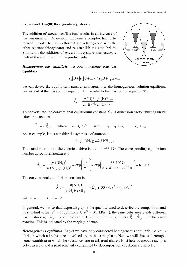
Water as solvent is treated as pure substance; therefore, it does not appear in the formula. Dilution with water lowers the concentration of the complex, but also the concentrations of the free ions. Therefore, the denominator will decrease much faster than the numerator. Be-cause the quotient is a constant, the so-called equilibrium number c

○K , the numerator has to

also decrease: The equilibrium is displaced towards the reactant side, i.e. some iron thiocy-anate complex has to decompose again into iron hexaquo complex cations and thiocyanate anions. The pale orange colour of the resulting solution is caused by the iron hexaquo com-plex. If, for example, Fe3+ or SCN– solutions are added to the pale orange dilute iron thiocyanate solution, it will turn red both times.


16

Experiment: Iron(III) thiocyanate equilibrium The addition of excess iron(III) ions results in an increase of the denominator. More iron thiocyanate complex has to be formed in order to use up this extra reactant (along with the other reactant thiocyanate) and re-establish the equilibrium. Similiarly, the addition of excess thiocyanate also causes a shift of the equilibrium to the product side. Homogenous gas equilibria. To obtain homogeneous gas equilibria

B C D EB C ... D E ...ν ν ν ν+ + + + we can derive the equilibrium number analogously to the homogeneous solution equilibria, but instead of the mass action equation 1´, we refer to the mass action equation 2´:

D E

CB

r r

r r

(D) (E) ...(B) (C) ...

ν ν

p νν

p pp p

⋅ ⋅=

⋅ ⋅

○K .

To convert into the conventional equilibrium constant pK

○ a dimension factor must again be

taken into account:

p pK κ=○ ○

K , where κ = (p) pν with νp = νB + νC + ... + νD + νE + ... . As an example, let us consider the synthesis of ammonia:

2 2 3N |g 3H |g 2 NH |g+ .

The standard value of the chemical drive is around +33 kG. The corresponding equilibrium number at room temperature is

2 35r 3

3 1r 2 r 2

(NH ) 33 10 Gexp exp 6.1 10(N ) (H ) 8.314 G K 298 K−

⎛ ⎞ ⎛ ⎞⋅⎜ ⎟= = = = ⋅⎜ ⎟⎜ ⎟⋅ ⋅ ⋅⎝ ⎠⎝ ⎠

○○

pp

p p RTA

K .

The conventional equilibrium constant is

22 23

32 2

(NH ) (100 kPa) 61 kPa(N ) (H )

− −= = ⋅ =⋅

○ ○p p

pKp p

K

with νp = −1 − 3 + 2 = −2. In general, we notice that, depending upon the quantity used to describe the composition and its standard value (c = 1000 mol⋅m−3, p = 101 kPa ...), the same substance yields different basic values cμ

○ , pμ○ ... and therefore different equilibrium numbers c

○K , p

○K ... for the same

reaction. This is indicated by the varying indexes. Heterogeneous equilibria. As yet we have only considered homogeneous equilibria, i.e. equi-libria in which all substances involved are in the same phase. Next we will discuss heteroge-neous equilibria in which the substances are in different phases. First heterogeneous reactions between a gas and a solid reactant exemplified by decomposition equilibria are selected.


17

Decomposition equilibria. In the case of the decomposition reaction of calcium carbonate described by

3 2CaCO |s CaO|s CO |g+ in a closed system two pure solid phases (CaCO3 und CaO) and a gas phase are in equilib-rium. The mass action equation 2´ is applied for the gas carbon dioxide. But how can we take pure solid substances (or pure liquids) B into account? In the case of these substances, the mass action term RTlncr(B) is omitted, i.e., μ(B) = μ○ (B); the pure solid substance does not appear in the mass action law. In a dilute solution this is also valid for the solvent which can be treated as a pure substance (see section 5.3). The equilibrium number p

○K for the decomposition of carbonate is therefore equal

r 2(CO )p p=○

K with

3 2(CaCO ) (CaO) (CO )exp exppμ μ μ

RT RT

⎛ ⎞⎛ ⎞ − −⎜ ⎟⎜ ⎟= =⎜ ⎟⎜ ⎟

⎝ ⎠ ⎝ ⎠

○ ○ ○ ○○ A

K .

The conventional equilibrium constant results in

2(CO )pK p=○

. The equilibrium constant is identical with the decomposition pressure, i.e. the pressure of car-bon dioxide at equilibrium, and hence not dependent on the amounts of the solid substances. Even though the pure solid substances do not appear in the mass action law they have to be present for establishing the equilibrium. The decomposition pressure depends, however, (like the equilibrium constant) on the temperature (see also section 4.5). When the calcium carbonate is, however, heated in an open system like a lime kiln, the gas escapes in the surroundings, the equilibrium is not established and the whole carbonate de-composes. In the same way the decomposition of crystalline hydrates etc. can be described. The approach can not only be applied on heterogeneous chemical reactions but also on transi-tions with a change of state of aggregation. Phase transitions. The evaporation of water represents an example for a phase transition with participation of a gas. The equilibrium number p

○K for the equilibrium between liquid water

and water vapour in a closed system,

2 2H O|l H O|g ,

results in

r 2(H O|g)p p=○

K .


18

Liquid water as pure liquid does not appear in the equation. The corresponding conventional equilibrium constant is

2(H O|g)pK p=○

. Hence, the equilibrium constant represents the vapour pressure of water, i.e. the pressure of water vapour in equilibrium with liquid water at the temperature considered. But we will discuss phase transitions in more detail in chapter 10. Our next topic are heterogeneous solution equilibria. Solubility of (ionic) solids. A substance submerged in a liquid will generally begin to dis-solve. The extremely low chemical potential μ of this substance in the pure solvent rises rap-idly − for c → 0, we know that μ → −∞ − with increasing dissolution and therefore concentra-tion. The process stops when the chemical potential of the substance in the solution is equal to that of the solid, i.e. equilibrium rules. We then refer to the solution as saturated, i.e. the solu-tion contains as much dissolved material as possible under given conditions (temperature, pressure, such as standard conditions). If the substance dissociates on dissolution, like a salt in water

AB|s A |w B |w+ −+

then the products of the dissociation together compensate for the dissolution drive of the salt AB:

(AB) (A ) (B )μ μ μ+ −= + .

We obtain for the equilibrium number

sp r r(A ) (B )c c+ −= ⋅○

K with

+

sp(AB) (A ) (B )exp exp μ μ μ

RT RT

−⎛ ⎞ ⎛ ⎞− −⎜ ⎟ ⎜ ⎟= =⎜ ⎟ ⎜ ⎟⎝ ⎠ ⎝ ⎠

○ ○ ○ ○○ A

K ,

as long as some undissolved AB is present, because the mass action term for the solid is omit-ted. Thus, the product of the relative concentrations of the ions in a saturated solution is con-stant. The value K

○ for the process of dissolving receives its own name, solubility product

(This is indicated by the index sp: sp○

K ). If a substance dissociates into several ions, then sp○

K consists of the corresponding number of factors. If the concentration c(A+) of one the products of dissociation decreases, the concentration of the second c(B−) must rise in order to maintain equilibrium (assuming the concentrations are small enough). If, as the result of some intervention, the product cr(A+)⋅cr(B−) rises above the value sp

○K , the substance AB is separated from the solution. As an example, we consider a

saturated table salt solution in which solid NaCl is in equilibrium withits ions in the solution:

NaCl|s Na |w Cl |w+ −+ .

The heterogeneous equilibrium can be described by the solubility product:


19

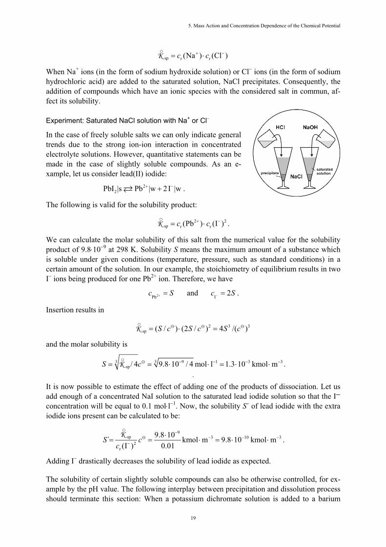
sp r r(Na ) (Cl )c c+ −= ⋅○

K When Na+ ions (in the form of sodium hydroxide solution) or Cl− ions (in the form of sodium hydrochloric acid) are added to the saturated solution, NaCl precipitates. Consequently, the addition of compounds which have an ionic species with the considered salt in commun, af-fect its solubility. Experiment: Saturated NaCl solution with Na+ or Cl− In the case of freely soluble salts we can only indicate general trends due to the strong ion-ion interaction in concentrated electrolyte solutions. However, quantitative statements can be made in the case of slightly soluble compounds. As an e-xample, let us consider lead(II) iodide:

22PbI |s Pb |w 2I |w+ −+ .

The following is valid for the solubility product:

2 2sp r r(Pb ) (I )c c+ −= ⋅

○K .

We can calculate the molar solubility of this salt from the numerical value for the solubility product of 9.8⋅10−9 at 298 K. Solubility S means the maximum amount of a substance which is soluble under given conditions (temperature, pressure, such as standard conditions) in a certain amount of the solution. In our example, the stoichiometry of equilibrium results in two I− ions being produced for one Pb2+ ion. Therefore, we have

2Pbc S+ = and

I2c S− = .

Insertion results in

2 3 3sp ( / ) (2 / ) 4 /( )S c S c S c= ⋅ =

○K

and the molar solubility is

3 9 1 3 33sp/ 4 9.8 10 / 4 mol l 1.3 10 kmol m− − − −= = ⋅ ⋅ = ⋅ ⋅

○S cK .

.

It is now possible to estimate the effect of adding one of the products of dissociation. Let us add enough of a concentrated NaI solution to the saturated lead iodide solution so that the I− concentration will be equal to 0.1 mol⋅l−1. Now, the solubility S´ of lead iodide with the extra iodide ions present can be calculated to be:

9sp 3 10 3

2r

9.8 10´ kmol m 9.8 10 kmol m(I ) 0.01

−− − −

−

⋅= = ⋅ = ⋅ ⋅

○

S cc

K . Adding I− drastically decreases the solubility of lead iodide as expected. The solubility of certain slightly soluble compounds can also be otherwise controlled, for ex-ample by the pH value. The following interplay between precipitation and dissolution process should terminate this section: When a potassium dichromate solution is added to a barium


20

chloride solution, a yellow precipitate of slightly soluble barium chromate is formed accord-ing to

2 22 7 2 42 Ba |w Cr O |w H O|l 2 BaCrO |s 2 H |w+ − ++ + + .

More precisely, the concentrations of the initial substances decrease, i.e barium chromate pre-cipitates until equilibrium is established according to the mass action law

( )( ) ( )

2

r22 2-

r r 2 7

H

Ba Cr Oc

c

c c

+

+=

○Κ .

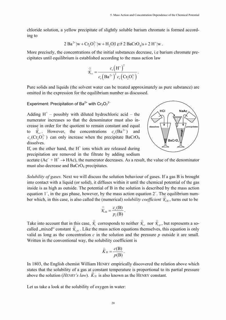
Pure solids and liquids (the solvent water can be treated approximately as pure substance) are omitted in the expression for the equilibrium number as discussed. Experiment: Precipitation of Ba2+ with Cr2O7

2−

Adding H+ – possibly with diluted hydrochloric acid – the numerator increases so that the denominator must also in-crease in order for the quotient to remain constant and equal to c

○K . However, the concentrations )Ba( 2

r+c and

)OCr( 272r

−c can only increase when the precipitate BaCrO4 dissolves. If, on the other hand, the H+ ions which are released during precipitation are removed in the filtrate by adding sodium acetate (Ac− + H+ → HAc), the numerator decreases. As a result, the value of the denominator must also decrease and BaCrO4 precipitates. Solubility of gases. Next we will discuss the solution behaviour of gases. If a gas B is brought into contact with a liquid (or solid), it diffuses within it until the chemical potential of the gas inside is as high as outside. The potential of B in the solution is described by the mass action equation 1´, in the gas phase, however, by the mass action equation 2´. The equilibrium num-ber which, in this case, is also called the (numerical) solubility coefficient H

○K , turns out to be

r

Hr

(B)(B)

cp

=○

K .

Take into account that in this case,

○K corresponds to neither c

○K nor p

○K , but represents a so-

called „mixed“ constant pc○

K . Like the mass action equations themselves, this equation is only valid as long as the concentration c in the solution and the pressure p outside it are small. Written in the conventional way, the solubility coefficient is

H(B)(B)

cKp

=○

. In 1803, the English chemist William HENRY empirically discovered the relation above which states that the solubility of a gas at constant temperature is proportional to its partial pressure above the solution (HENRY’s law). HK

○ is also known as the HENRY constant.

Let us take a look at the solubility of oxygen in water:


21

2 2O |g O |w . In this case, the standard value of the chemical drive is –16.4 kG. The (numerical) solubility coefficient at room temperature is equal to

33r 2

H 1r 2

(O ) 16.4 10 Gexp exp 1.3 10(O ) 8.314 G K 298 K

−−

⎛ ⎞ ⎛ ⎞− ⋅⎜ ⎟= = = = ⋅⎜ ⎟⎜ ⎟ ⋅ ⋅⎝ ⎠⎝ ⎠

○○ c

p RTA

K ,

while the conventional one results in

35 3 12

H H2

(O ) 1 kmol m 1.3 10 mol m Pa(O ) 100 kPa

−− − −⋅

= = ⋅ = ⋅ ⋅ ⋅○ ○cK

pK .

The partial pressure of O2 in air is about 20 kPa. For O2 concentration in air-saturated water at 298 K, we obtain

5 3 1 3 3Hr 2 2(O ) (O ) 1.3 10 mol m Pa 20 10 Pa 0.26 mol mc K p − − − −= ⋅ = ⋅ ⋅ ⋅ ⋅ ⋅ = ⋅

○.

Concentrations of O2 in waters which are important to biological processes can be estimated in this way. Distribution equilibria. Relations that can be dealt with in a theoretically similar way would be, for example, systems where a third substance B (possibly iodine) is added to two practi-cally immiscible liquids such as water/ether. Iodine is soluble in both liquid phases (´) and (´´). Substance B disperses between these phases until its chemical potential is equal in both. The equilibrium number is then:

rN

r

(B)´́(B)´

cc

=○

K

where

N(B)´ (B)´́exp exp μ μ

RT RT

⎛ ⎞ ⎛ ⎞−⎜ ⎟ ⎜ ⎟= =⎜ ⎟ ⎜ ⎟⎝ ⎠ ⎝ ⎠

○ ○ ○○ A

K .

Conventionally, we obtain

N(B)´́(B)´

cKc

=○

.

The ratio of equilibrium concentrations (or the mole fractions, etc.) of the dissolved substance in two liquid phases is, in the case of small concentrations, a temperature dependent constant (NERNST’s distribution law). The constant NK

○is also called NERNST’s distribution coefficient.

Distribution equilibria play a significant role in separating the substances in a mixture by the process of extraction. The laboratory procedure called „extraction by shaking“ (extracting a substance from its solution) by using another solvent in which the substance dissolves much better, is based on such equilibria. This method can be used to completely remove iodine from water by repeatedly extracting it with ether. Partition chromatography is based upon the same principle. A solvent acts as the stationary phase in the pores of a solid carrier material (paper


22

for example) and a second solvent (with the substance mixture to be separated) flows past it in the form of a mobile phase. This is known as a mobile solvent. The more soluble a substance is in the stationary phase, the longer it will remain there and the more strongly its movement along this phase will slow down. Eventually a separation occurs in the mixture originally ap-plied at a point. Influence of temperature. The equilibrium numbers (and constants) we have considered so far are valid only under certain circumstances (mostly standard conditions at 298 K and 101 kPa). If the value of K at an arbitrary temperature is of interest, then the RT term as well as the tem-perature dependence of chemical drive A need to be taken into account. We refer here to the linear approximation introduced in Section 4.2:

0 0( )T T= + −A A α .

Insertion into the equation above yields the following result for the equilibrium number at a temperature T

0 0( ) ( )( ) exp T T TTRT

⎛ ⎞+ −⎜ ⎟=⎜ ⎟⎝ ⎠

A○

○ αK .

When the temperature is increased (ΔT > 0), ( )T○

K can increase or decrease relative to the initial value 0( )T

○K depending upon the values of A

○(T0) and α which are typical for a particu-

lar reaction. In the first case, the equilibrium composition shifts to benefit the products and in the second case, it shifts to benefit the initial substances. The equilibrium constant can be in-fluenced by the choice of temperature. This can be of great importance for large-scale techni-cal reactions as well as for environmentally relevant ones.

5.7 Potential diagrams of dissolved substances Energy must be used in order to transfer matter from a state of low μ value to a state of high μ value. Therefore, the potential μ can be regarded as a kind of energy level the matter is on. This is why matter with a high chemical potential is often called energy rich and matter with low potential, energy poor. These terms are not to be considered absolute in themselves but only in relation to other substances with which the substance in question can reasonably be compared. When the amount n of a dissolved substance in a given volume is continuously increased, the potential μ of the substance also increases. While at first, only small changes Δn in the amount of substance are enough to cause a certain rise in potential Δμ, later on increasingly large amounts are necessary for this. As long as the concentration is not too high, the mass action equation remains valid. This means that the concentrations (or when the volume re-mains constant, the amount), must always increase by the same factor b if μ is to increase by the same amount. n therefore increases exponentially along with the chemical potential μ. The example of an electric capacitor can be used to characterize the capacity of a substance. The chemical capacity B is defined by the following equation:


23

dd

nBμ

= .

A well known example of the quantity B is the so-called buffering capacity, meaning the ca-pacity

HB + of a given amount of a solution for hydrogen ions. This will be gone into in more

detail in Chapter 6.6. If the region being dealt with is homogeneous, B can logically be related to the volume:

BV

=b .

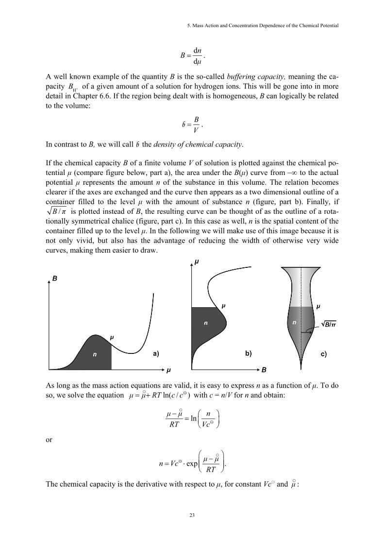
In contrast to B, we will call b the density of chemical capacity. If the chemical capacity B of a finite volume V of solution is plotted against the chemical po-tential μ (compare figure below, part a), the area under the B(μ) curve from −∞ to the actual potential μ represents the amount n of the substance in this volume. The relation becomes clearer if the axes are exchanged and the curve then appears as a two dimensional outline of a container filled to the level μ with the amount of substance n (figure, part b). Finally, if

/B π is plotted instead of B, the resulting curve can be thought of as the outline of a rota-tionally symmetrical chalice (figure, part c). In this case as well, n is the spatial content of the container filled up to the level μ. In the following we will make use of this image because it is not only vivid, but also has the advantage of reducing the width of otherwise very wide curves, making them easier to draw.

As long as the mass action equations are valid, it is easy to express n as a function of μ. To do so, we solve the equation ln( / )μ μ RT c c= +

○ with c = n/V for n and obtain:

lnμ μ nRT Vc− ⎛ ⎞= ⎜ ⎟

⎝ ⎠

○

or

exp μ μn VcRT

⎛ ⎞−⎜ ⎟= ⋅ ⎜ ⎟⎝ ⎠

○ .

The chemical capacity is the derivative with respect to μ, for constant Vc and μ○ :


24

expVc μ μ nBRT RT RT

⎛ ⎞−⎜ ⎟= ⋅ =⎜ ⎟⎝ ⎠

○

.

As a consequence, B, like n, depends exponentially upon μ. In this case, the container whose curve we are interested in has the form of an „exponential horn“ which is open at the top. The chemical capacity density b can be easily calculated from B:

expB c μ μ cV RT RT RT

⎛ ⎞−⎜ ⎟= = ⋅ =⎜ ⎟⎝ ⎠

○

b

.

Again, it depends exponentially on µ. We will take a closer look at this approach using the example of glucose. In its solid and pure state, glucose has a chemical potential which is not subject to mass action. For this reason, it is represented as a horizontal line in the potential diagram. Because, as previously stated, glucose occurs in two forms, α and β, two potential levels lying close together should actually be drawn in. However, for the sake of simplicity, only one is represented here.

In the dissolved state and depending upon concentra-tion or amount, we have an entire band of potential val-ues. Instead of the band, we will use the B(μ) curve as it is described for the general case above to express this dependence. Alternatively, we can use the b(μ) curve, which looks identical to it. The radius of the rotation-ally symmetrical chalice equals / πb . Therefore,

the contents up to a chosen level equal the quantity of glucose present there relative to the volume of solution. This means it is equal to the total concentration of glucose. At small con-centrations, the radius increases exponentially with rising μ; for high concentrations, this is only approximate. We do not need to differentiate between the α and the β forms because an equilibrium rather quickly develops between the two isomers. The basic value of the potential applies to this equilibrium mixture. The contents of the chalice have been drawn to this arbi-trarily chosen potential level. We will also generally choose this fill level for other substances. The value in a living organism would be considerably lower, though. If the amount of dissolved glucose were to be continuously increased, and the fill level of the chalice raised to the level of the solid glucose, the glucose would begin to crystallize. At the same time, the glucose would begin to run over the rim of the chalice. If, on the other hand, solid glucose were present, it would need to dissolve for as long as it would take for all the crystals to disappear or until the potential in the solution increased to the level of the chalice


25

rim in the drawing. One might say that in this state, the glucose solution is saturated relative to the solid.

Mass Action and Concentration Dependence of the Chemical Potential

Documents

Transcript of Mass Action and Concentration Dependence of the Chemical Potential