O(4)-symmetric position-space renormalization of lattice operators

Masaaki Tomii1, ∗ and Norman H. Christ1

1Physics Department, Columbia University, New York 10027, USA

Abstract

We extend the position-space renormalization procedure, where renormalization factors are cal-

culated from Green’s functions in position space, by introducing a technique to take the average of

Green’s functions over spheres. In addition to reducing discretization errors, this technique enables

the resulting position-space correlators to be evaluated at any physical distance, making them con-

tinuous functions similar to the O(4)-symmetric position-space Green’s functions in the continuum

theory but with a residual dependence on a regularization parameter, the lattice spacing a. We

can then take the continuum limit of these renormalized quantities calculated at the same physical

renormalization scale |x| and investigate the resulting |x|-dependence to identify the appropriate

renormalization window.

As a numerical test of the spherical averaging technique, we determine the renormalized light

and strange quark masses by renormalizing the scalar current. We see a substantial reduction of

discretization effects on the scalar current correlator and an enhancement of the renormalization

window. The numerical simulation is carried out with 2 + 1-flavor domain-wall fermions at three

lattice cutoffs in the range 1.79–3.15 GeV.

∗ mt3164˙at˙columbia.edu

1

arX

iv:1

811.

1123

8v1

[he

p-la

t] 2

7 N

ov 2

018

I. INTRODUCTION

Operator renormalization is necessary to calculate many quantities such as weak matrix

elements using lattice simulation. So far, several different methods to renormalize lattice

operators have been proposed, applied and improved. Since each method has individual

advantages and disadvantages, we can use the method that is the most convenient for our

situation and purpose.

In this work, we focus on the position-space procedure [1, 2], in which the renormalization

condition for an operator is imposed on the corresponding correlation function in position

space. It is an important advantage of this procedure that it provides a fully gauge invariant

renormalization prescription since the correlator used in the renormalization condition is

gauge invariant. This advantage prevents the mixing with gauge noninvariant operators that

occurs in gauge noninvariant schemes such as the regularization independent momentum

subtraction (RI/MOM) scheme [3]. Since the operators appearing in the position-space

renormalization prescription are evaluated at separated space-time points, operators which

vanish when the equations of motion are imposed will also not contribute. Therefore a

position-space renormalization scheme will also avoid mixing with operators which vanish

by the equations of motion – mixing which can occur in the RI/MOM approach.

An important difficulty of the position-space approach arises from the discrete lattice of

points on which the position space Green’s function is evaluated. Unless one works with

lattices whose lattices spacings are related as integer multiples, errors may be introduced

when combining results from two different ensembles. Combining results from ensembles

with different lattice spacing is necessary both when evaluating the continuum limit and

when using step scaling [4–6]. (For example, when Cichy et al. [7] employ step scaling in

position space they consider lattice spacings which differ by factors of two.) Recall that step

scaling is an important nonperturbative method used to relate the normalization of operators

that are being used in a coarse lattice calculation to physically equivalent operators defined

on a fine, weak-coupling lattice where a connection to perturbatively normalized operators

can be more accurately made.

In an RI/MOM scheme the Fourier transform averages over the discrete lattice and

the resulting functions of momentum approach their continuum limits in a well-understood

fashion [8, 9]. In this paper we propose an alternative average that partially smooths the

2

discrete nature of the position-space lattice while working with gauge invariant quantities

and maintaining a non-zero separation between the operators whose Green’s functions are

being studied.

Our strategy is best illustrated using two-point functions, which are the starting point of

the present position-space renormalization schemes, as illustrated by the expression

G(xn) =⟨O(xn)O(0)†

⟩(1)

where O is a gauge-invariant composite local operator, xn is a point on our discrete lattice

determined by the four integers n = (n1, n2, n3, n4) and, for simplicity, the second point 0

is chosen to be the origin, also a point of this lattice. As is described in more detail in Sec-

tion III, we begin by extending this function into a function G(x) of the continuous position

four-vector x, obtained by multi-linear interpolation from the sixteen values obtained by

evaluating G(xn) at the sixteen lattice points that lie at the vertices of the four-dimensional

cube which contains the point x.

Assuming, as we do throughout this paper, that our lattice theory has no order a errors,

our interpolated Green’s function G(x) will agree with the corresponding Green’s function

of the continuum theory up to errors which vanish as a2 in the continuum limit. Of course,

the a2 errors which appear in the piece-wise linear function G(x) will still reflect the O(4)

symmetry breaking of the underlying lattice. In order to reduce these lattice artifacts and

define a function of a single scale, we further simplify our Green’s function by averaging the

point x over a three-dimension sphere of radius |x| centered at the origin:

G(|x|) =1

2π2|x|3

∫d4x′ δ

(|x′| − |x|

)G(x′). (2)

We will then impose conditions on G(|x|) to renormalize the operator O.

The finite lattice spacing errors that are present in the lattice Green’s function G(xn) are

expected to appear as simple polynomials in a with coefficients which in perturbation theory

depend only logarithmically in a, allowing a simple exptrapolation to the continuum limit.

The lattice spacing dependence of our averaged quantity G(|x|) will be more complicated.

In addition to the simple a2 errors coming from G(xn), the sphere averaging procedure will

introduce O(a2) errors which, while bounded by a2 may be complicated irregular functions of

a which could cause an explicit extrapolation in a2 to fail. As will be shown in Appendix A,

this irregular dependence on a appears to be negligible, making the scheme proposed here

3

suitable for a calculation in which the continuum limit is to be evaluated. Of course, were

this error too large, we may be able to introduce a higher-order interpolation scheme which

would make these troubling effects of higher order than a2 and therefore systematically

negligible.

As an example of the spherical average, we present our result for the quark mass renormal-

ization, which can be done by renormalizing the scalar current. There are several previous

works on position-space renormalization of bilinear operators [2, 10, 11]. For renormalization

of bilinear operators, there is another important advantage of the position-space procedure:

the perturbative matching to the modified minimal subtraction (MS) scheme is available to

O(α4s) for the vector, axial-vector, scalar and pseudoscalar currents and to O(α3

s) for the

tensor current [12]. Utilizing the spherical averaging technique, we perform a new analysis

that takes the continuum limit of the renormalized quark mass at many values of |x| and

shows its |x|-dependence. The final result agrees with the FLAG average [13] as well as our

previous result using the RI/SMOM scheme [14, 15], an improved version of the RI/MOM

scheme with reduced sensitivity to long-distance effects, for the same ensembles [16].

An important future use for this sphere-averaged position-space renormalization scheme

is to accurately define the weak operators which are needed in the calculation of non-leptonic

decays, such as the K → ππ decay, in a three-flavor theory. At present these three-flavor

operators are determined by using QCD perturbation theory to calculate that combination

of three-flavor operators which will give the same matrix elements as the more physical

four-flavor operators when evaluated at energies below the charm threshold. Such a use

of QCD perturbation theory below the charm threshold introduces uncontrolled system-

atic errors. However, a nonperturbative matching of three- and four-flavor operators using

RI/MOM methods is also potentially uncertain. The gauge-noninvariant operators that are

traditionally neglected in RI/MOM calculations when performed at higher energies because

of the presence of explicit factors of the gluon field, may give large contributions at energies

below the charm mass. The sphere-averaged position-space renormalization scheme may

allow a nonperturbative determination of the three-flavor Wilson coefficients in which the

only errors, which are systematically improvable, come from the neglect of higher-dimension

operators proportional to inverse powers of the charm quark mass.

The paper is organized as follows. In Section II, we summarize the traditional procedure

of the position-space renormalization of an operator that does not mix with any other

4

operator and identify the problem posed by the discretization errors that is addressed by

the method presented in this paper. Our core technique in this work, the spherical average,

is introduced in Section III. In Section IV, a concrete strategy to calculate the renormalized

quark mass through the position-space renormalization of the scalar current is proposed.

In Section V, the details of the numerical simulation is described. In Section VI, our final

result for the renormalized quark mass is shown. In the process, we show the performance

of the spherical average especially at short distances and discuss how the renormalization

window can be extended. In addition, we present a test of an ad hoc prescription to reduce

nonperturbative effects at long distances that are mainly due to instanton interactions. In

Section VII, we summarize the paper and discuss the prospect of further applications of the

spherical average for various quantities calculated on the lattice. In Appendix A, we describe

our investigation of the irregular a-dependence that appears in the spherical average, which

turns out to be negligible.

II. FUNDAMENTAL PROCEDURE IN PREVIOUS WORKS

In this section, we summarize the traditional approach to position-space renormalization

of an operator that does not mix with any other operator. We consider two-point Green’s

functions of a composite operator Os(µ;x) renormalized at a scale µ in a scheme s and the

corresponding lattice operator Olat(1/a; an) for a lattice spacing a,

GsO(µ;x) =

⟨Os(µ;x)Os(µ; 0)†

⟩, Glat

O (1/a; an) =⟨Olat(1/a; an)Olat(1/a; 0)†

⟩. (3)

Here, we distinguish a four-dimensional point in the continuum theory x = (x1, x2, x3, x4)

from that on the lattice an = (an1, an2, an3, an4) since the discrete character of the lattice

points is carefully considered throughout the paper. In this section, we treat these two-point

functions in the chiral limit, which does not require consideration of the mass renormalization

of quarks in the correlators and remove an extra scale from the renormalization procedure.

An operator OX(µ;x) renormalized at µ in the X-space scheme [2, 10] is defined in the

continuum theory by the condition

GXO (µ;x)

∣∣µ=1/|x| = Gfree

O (x), (4)

where GfreeO (x) is the corresponding two-point Green’s function evaluated in free field theory

and |x| =√∑

µ x2µ. Since this nonperturbative scheme is fully gauge invariant and free from

5

contact terms unlike the RI/MOM scheme, it prevents mixing with irrelevant operators and

thus is a quite convenient scheme especially at low energies where perturbative schemes are

not applicable and mixing with many irrelevant operators can occur in gauge noninvariant

schemes.

The traditional renormalization condition

ZX/latO (µ, 1/a; an)

2∣∣µ=1/a|n|G

latO (1/a; an) = Gfree

O (x)∣∣x=an

, (5)

yields

ZX/latO (µ, 1/a; an)

∣∣µ=1/a|n| =

√GfreeO (x)

∣∣x=an

GlatO (1/a; an)

, (6)

which violates rotational symmetry and depends on n in a complicated way. Since the

O(4)-violating n-dependence is O(a2), it can be eliminated and only the dependence on

the distance scale µ = 1/a|n| remains if the continuum limit of the renormalized operator

ZX/latO (µ, 1/a; an)Olat(1/a; an′) is accurately taken. However, evaluating the continuum limit

requires an a2 extrapolation of numerical values at a fixed physical location x = aAnA =

aBnB = . . . so that when comparing ensembles A and B it is only the lattice spacing, not

the physical position which is changing. This means the ratios of the lattice spacings for

the ensembles used to evaluate the continuum limit need to be integers or simple rational

numbers. However, lattice spacings are not tuned so precisely in practical simulations. We

propose a way to circumvent this problem in the next section.

We close the section by describing the relation between operators in the X-space scheme

and those in another scheme s. Using Eqs. (3) and (4), the matching factor Zs/XO (µ, µ′),

which is defined by Os(µ;x) = Zs/XO (µ, µ′)OX(µ′;x), can be written as

Zs/XO (µ, µ′) =

√GsO(µ;x)

GfreeO (x)

∣∣∣∣∣|x|=1/µ′

. (7)

If we already know the correlator in the scheme s and any treatments in the X-space scheme

such as the step scaling are not needed, we can skip renormalizing operators to the X-space

scheme and directly compute

Zs/latO (µ, 1/a; an) ≡ Z

s/XO (µ, µ′)Z

X/latO (µ′, 1/a; an)

∣∣µ′=1/a|n| =

√GsO(µ;x)

∣∣x=an

GlatO (1/a; an)

. (8)

Of course, this expression violates rotational symmetry as does Eq. (6) and therefore suffers

from the same difficulty in taking the continuum limit of the corresponding renormalized

operator as is described above.

6

III. SMOOTHING AVERAGE OVER SPHERES

Renormalization factors determined through the procedure discussed in the previous sec-

tion contain discretization errors which depend in a complicated way on the lattice point n

where the renormalization condition is imposed due to the violation of rotational symme-

try. The complicated discretization errors induce difficulty in taking the continuum limit of

renormalized operators as mentioned in the previous section. Some ideas to reduce this kind

of discretization errors, subtracting free-field discretization error [2, 11] and discarding the

lattice data points where discretization errors are quite large [10, 17], have been applied.

These previous works usually naıvely averaged the renormalization factor Eq. (8) over lattice

points in the renormalization window, which could induce an irrelevant linear dependence

on a and further degrade the accuracy of the continuum extrapolation of a renormalized

quantity which assumed that the leading discretization error is O(a2). In this section, we

propose another way to smooth lattice results, in which the irrelevant O(a1) discretization

error does not appear and the continuum extrapolation of a renormalized quantity using a

constant plus an O(a2) term can be safely taken.

We consider a lattice quantity fa,n calculated at each lattice point n. The a-dependence

of fa,n can be sketched as

fa,n = F (x; a)|x=an + ca,na2 +O(a4), (9)

with a coefficient ca,n which depends on the lattice point n in a complicated way. In the

simplest case, F (x; a) is the continuum limit of the quantity being computed and does not

depend on a. However, by including a possible logarithmic a-dependence, we can make our

discussion more general and include the case where fa,n is an n-dependent renormalization

factor such as the quantities given in Eqs. (6) and (8) or a correlator of unrenormalized

operators.

We start with the case of one dimension, where we assume x = x1. We then use linear

interpolation to extend the lattice results for fa,n, to define a function fa(x) for all values of

the continuous physical distance x:

fa(x) =(a(n+ 1)− x)fa,n + (x− an)fa,n+1

a, (10)

where n is now defined as bx/ac, the largest integer that is less than or equal to x/a.

Inserting Eq. (9) into this equation and expanding F (an; a) and F (a(n+1); a) around x, we

7

see that fa(x) is an approximation to F (x; a) as a continuous function of x that is accurate

up to O(a2). Note that the appropriate weight of a(n + 1) − x and x − an in Eq. (10)

is important to avoid introducing an O(a1) error which would spoil the accuracy of an a2

continuum extrapolation.

In the case of two dimensions, the weighted average Eq. (10) can be modified to a bilinear

interpolation

fa(x) = a−2( a(n1 + 1)− x1 x1 − an1 )

fa,n fa,n+2

fa,n+1 fa,n+1+2

a(n2 + 1)− x2x2 − an2

, (11)

where nµ = bxµ/ac and µ is the unit vector for the µ-direction. While this weighted average

is also easily found to be free from the O(a1) error, it is expected to depend significantly

on the direction of x as well as the distance |x| due to the violation of rotational symmetry.

The most naıve way to smooth this discretization error may be to introduce the average

over a circle with the radius of |x|,

fa(|x|) =1

2π

∫ 2π

0

dθ fa(x), (12)

where we use two-dimensional polar coordinates

x1 = |x| cos θ, x2 = |x| sin θ. (13)

The extension to four dimensions is straightforward. The interpolation of fa at x is given

by

fa(x) = a−41∑

i,j,k,l=0

∆1,i∆2,j∆3,k∆4,l fa,n+i1+j2+k3+l4, (14)

where we define the factors

∆µ,i = |a(nµ + 1− i)− xµ|. (15)

One can easily verify this interpolated value is also free from the O(a1) error. The smoothing

average over the four-dimensional sphere with the radius of |x| is

fa(|x|) =1

2π2

∫ π

0

dθ1

∫ π

0

dθ2

∫ 2π

0

dθ3 sin2 θ1 sin θ2 fa(x), (16)

8

with four-dimensional polar coordinates

x1 = |x| cos θ1,

x2 = |x| sin θ1 cos θ2,

x3 = |x| sin θ1 sin θ2 cos θ3,

x4 = |x| sin θ1 sin θ2 sin θ3. (17)

The averaged quantity fa(|x|) will differ from the direction independent continuum quantity

F (x; a) by discretization errors of O(a2).

Although the discretization error of the spherical average is thus O(a2), it should be

noted that the averaged value is not a regular polynomial in a but will contain extra non-

differentiable terms of O(a2) because of the complicated a-dependence of the floor function

nµ = bxµ/ac. This irregularity could arise also from the fact that the set of the lattice

points n and their weight used by the spherical average at each fixed physical distance |x|

depend on the lattice spacing a. Such complicated a-dependence could spoil the accuracy

of a continuum extrapolation which assumed a regular a2 term. In Appendix A, we discuss

the significance of such complicated a-dependence and demonstrate it is small.

IV. QUARK MASSES RENORMALIZATION IN POSITION SPACE

A. Strategy

Since the quark mass renormalization factor Zm can be calculated as the inverse of the

renormalization factor ZS of the scalar current S(x) = u(x)d(x), we consider the renormal-

ization of S(x), which is equivalent to that of the pseudoscalar current P (x) = u(x)iγ5d(x)

as long as chiral symmetry on the lattice is maintained. Since we use domain-wall fermions,

we can calculate Zm from the renormalization of S(x) and P (x).

In what follows, we employ the MS scheme and introduce the input light quark mass

parameter m′ud that is used for the calculation of the correlators on the lattice. The n-

dependent renormalization factor Eq. (8) is then rewritten as

ZMS/latS/P (µ, 1/a; an;m′ud) =

√√√√ GMSS (µ;x; 0)

∣∣x=an

GlatS/P (1/a; an;m′ud)

. (18)

9

The chiral limit (m′ud → 0) is taken in Section VI. In this work, the scalar correlator GMSS in

continuum perturbation theory is considered only in the massless limit, where it is equivalent

to the pseudoscalar correlator and is available to O((αs/π)4) accuracy [12]. The strategy

to improve the convergence of the perturbative series of the correlator is discussed in the

following subsection and in [11] for more detail.

We also analyze an O(4)-symmetric renormalization factor

Z

MS/lat

S/P (µ, 1/a; |x|;m′ud) = ZMS/XS (µ, µ′)

ZX/lat

S/P (µ′, 1/a; |x|;m′ud) (19)

obtained from Eq. (7) and the O(4)-symmetric renormalization condition

ZX/lat

S/P (µ, 1/a; |x|;m′ud)2∣∣µ=1/|x|G

latS/P (1/a; |x|) = Gfree

S (x), (20)

with the sphere-averaged Green’s function GlatS (1/a; |x|) calculated as follows. It should be

noted that the complicated a-dependence appearing in the multi-linear interpolation depends

on the first and second derivatives of the continuum version of the function that is to be

interpolated with respect to |x|. Therefore, the spherical averaging procedure is applied to

a function whose |x|-dependence in the continuum limit is as small as possible. For this

reason, we calculate the spherical average of the ratio GlatS/P (1/a; an;m′ud)/G

freeS (x)|x=an at

each distance |x| and then define the sphere-averaged Green’s function GlatS (1/a; |x|) as the

product of it and GfreeS (x).

Note that either ZMS/latS/P (µ, 1/a; an;m′ud) or

Z

MS/lat

S/P (µ, 1/a; |x|;m′ud) may not be an ap-

propriate renormalization factor since it still depends on the location n or |x| due to the

following sources of error:

• Discretization effects in GlatS/P (1/a; an;m′ud).

• Truncation error from the perturbative calculation of GMSS (µ;x; 0).

• Nonperturbative QCD effects, which are not present in the perturbatively calculated

GMSS (µ;x; 0) but do appear in the nonperturbatively measured Glat

S/P (1/a; an;m′ud).

The first source is uncontrollable at short distances (|x|, a|n| ∼ a), while the others are

significant at long distances (|x|, a|n| & 1/ΛQCD). We need to find or create an appropri-

ate window where all of these sources of error are under control and the n-dependence of

ZMS/latS/P (µ, 1/a; an;m′ud) or |x|-dependence of

Z

MS/lat

S/P (µ, 1/a; |x|;m′ud) is sufficiently small.

10

Since the third source especially violates the degeneracy of ZMS/latS (µ, 1/a; an;m′ud) and

ZMS/latP (µ, 1/a; an;m′ud), analyzing both of these may specify the region where nonperturba-

tive effects are less significant.

Using the unrenormalized quark mass mbareq (1/a) at the physical pion mass, which is

given in Ref. [16] for the degenerate up and down quarks (q = ud) and the strange quark

(q = s) on our ensembles, we analyze the n- and |x|-dependent renormalized quark masses

mMSq,S/P (µ; an; a,m′ud) =

mbareq (1/a)

ZMS/latS/P (µ, 1/a; an;m′ud)

, (21)

and mMS

q,S/P (µ; |x|; a,m′ud) =mbareq (1/a)

ZMS/lat

S/P (µ, 1/a; |x|;m′ud), (22)

where q = ud, s.

In Section VI, we determine the renormalized mass of the degenerate up and down quarks

and the strange quark on our ensembles.

B. Scalar correlator in massless perturbation theory

While the available four-loop perturbative results is an important advantage of the

position-space renormalization of the scalar current, the region where discretization errors

may be under controlled is 1/|x| . 1 GeV for currently available lattices with domain-wall

fermions and therefore the convergence of the perturbative expansion might be still insuffi-

cient. The convergence can be improved by a resummation of the perturbative series using

the coupling constant at another renormalization scale as explained below.

Chetyrkin and Maier [12] gave the coefficients CS,CMi of the perturbative expansion

GMSS (µx;x; 0) =

3

π4|x|6

(1 +

∑i

CS,CMi as(µx)

i

), (23)

up to i = 4. Here, the strong coupling constant as(µx) = αs(µx)/π is renormalized in

the MS scheme at µx = 2e−γE/|x| ' 1.123/|x| with Euler’s constant γE = 0.5772 and is

evaluated using the scale of QCD ΛMSQCD = 332(17) [18] in three flavor theory. By setting the

renormalization scale µx of the scalar current and the strong coupling constant proportional

to |x|−1, the logarithmic |x|-dependence of the perturbative coefficients can be eliminated.

11

The anomalous dimension of the scalar current, which is the same as the mass anomalous

dimension except for the sign and is calculated up to the five-loop level [19], enables us to

evolve the scale on the LHS of Eq. (23). The beta function, which is also available to the

five-loop level [20], can be used to evolve the scale of the strong coupling constant on the

RHS of Eq. (23). Using the original perturbative coefficients CS,CMi and these scale evolution

procedures, we obtain a general expression of the perturbative series

GMSS (µ′x;x; 0) =

3

π4x6

(1 +

∑i

CSi (µ∗x, µ

′x)as(µ

∗x)i

), (24)

where µ′x and µ∗x are the renormalization scale of the scalar current and that of the strong

coupling constant, respectively. While the all-order calculation of the RHS is supposed

to be independent of µ∗x, any finite-order calculation does depend on µ∗x. Therefore, the

convergence of the perturbative series can be investigated by varying µ∗x.

Thus, we obtain the numerical value of the scalar correlator GMSS (µ′x;x; 0)

∣∣µ∗x

calculated

with a scale µ∗x of the strong coupling constant. In order to renormalize the scalar current

at a specific scale, which we set to 3 GeV, the scale evolution is needed from µ′x to 3 GeV,

GMSS (3 GeV;x; 0)

∣∣µ∗x,µ

′x

= exp

(−2

∫ as(3GeV)

as(µ′x)

dz

z

γm(z)

β(z)

)GMSS (µ′x;x; 0)

∣∣µ∗x

=

(ρ(as(µ

′x))

ρ(as(3 GeV))

)2

GMSS (µ′x;x; 0)

∣∣µ∗x, (25)

where γm(z) and β(z) are the mass anomalous dimension and the beta function, respectively,

and ρ(z) is known to the five-loop level [19]. While GMSS (3 GeV;x; 0)

∣∣µ∗x,µ

′x

is also supposed

to be independent of µ∗x and µ′x in an all-order calculation, the convergence can be optimized

by tuning the scale parameters µ′x and µ∗x so that the dependence on these scale parameters

is minimized. We use the optimal values µ′x = e0.8/|x| ' 2.2/|x| and µ∗x = e1.05/|x| ' 2.9/|x|

in the case of three-flavor QCD quoted by Ref. [11].

V. LATTICE SETUP

We perform lattice simulation with the ensembles of 2 + 1-flavor dynamical domain-wall

fermions [21, 22] and the Iwasaki gauge action [23, 24] generated by the RBC and UKQCD

collaborations [16]. Table I summarizes the properties of the ensembles used in this work.

We calculate with three lattice cutoffs ranging from 1.785(5) GeV to 3.148(17) GeV. The

12

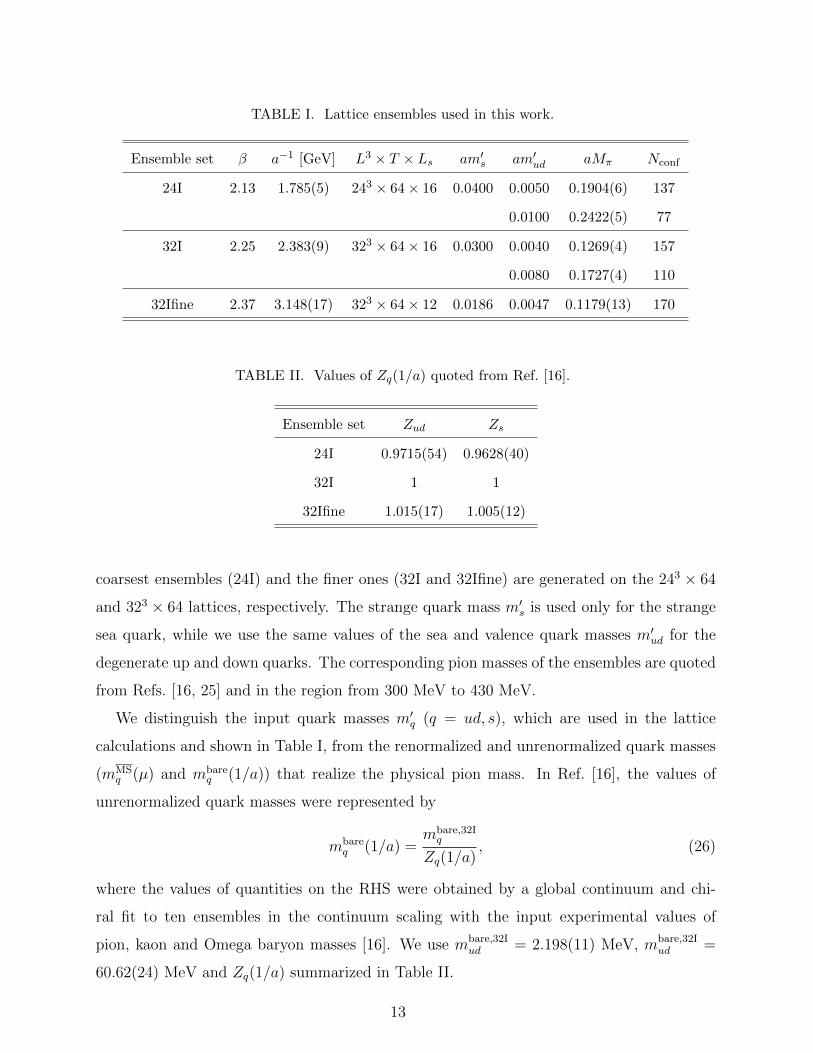
TABLE I. Lattice ensembles used in this work.

Ensemble set β a−1 [GeV] L3 × T × Ls am′s am′ud aMπ Nconf

24I 2.13 1.785(5) 243 × 64× 16 0.0400 0.0050 0.1904(6) 137

0.0100 0.2422(5) 77

32I 2.25 2.383(9) 323 × 64× 16 0.0300 0.0040 0.1269(4) 157

0.0080 0.1727(4) 110

32Ifine 2.37 3.148(17) 323 × 64× 12 0.0186 0.0047 0.1179(13) 170

TABLE II. Values of Zq(1/a) quoted from Ref. [16].

Ensemble set Zud Zs

24I 0.9715(54) 0.9628(40)

32I 1 1

32Ifine 1.015(17) 1.005(12)

coarsest ensembles (24I) and the finer ones (32I and 32Ifine) are generated on the 243 × 64

and 323 × 64 lattices, respectively. The strange quark mass m′s is used only for the strange

sea quark, while we use the same values of the sea and valence quark masses m′ud for the

degenerate up and down quarks. The corresponding pion masses of the ensembles are quoted

from Refs. [16, 25] and in the region from 300 MeV to 430 MeV.

We distinguish the input quark masses m′q (q = ud, s), which are used in the lattice

calculations and shown in Table I, from the renormalized and unrenormalized quark masses

(mMSq (µ) and mbare

q (1/a)) that realize the physical pion mass. In Ref. [16], the values of

unrenormalized quark masses were represented by

mbareq (1/a) =

mbare,32Iq

Zq(1/a), (26)

where the values of quantities on the RHS were obtained by a global continuum and chi-

ral fit to ten ensembles in the continuum scaling with the input experimental values of

pion, kaon and Omega baryon masses [16]. We use mbare,32Iud = 2.198(11) MeV, mbare,32I

ud =

60.62(24) MeV and Zq(1/a) summarized in Table II.

13

�

�

�

�

�

�� ���� ���� ���� ���� �� ���� ���������������

���

������

���

��������

�������� ���������

〜�

�

��

�

�

�

�

�

�� ���� ���� ���� ���� �� ���� ����

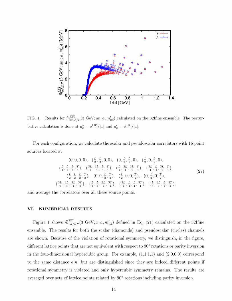
FIG. 1. Results for mMSud,S/P (3 GeV; an; a,m′ud) calculated on the 32Ifine ensemble. The pertur-

bative calculation is done at µ∗x = e1.05/|x| and µ′x = e0.80/|x|.

For each configuration, we calculate the scalar and pseudoscalar correlators with 16 point

sources located at

(0, 0, 0, 0), (L2, L2, 0, 0), (0, L

2, L2, 0), (L

2, 0, L

2, 0),

(L4, L4, L4, T4), (3L

4, 3L

4, L4, T4), (L

4, 3L

4, 3L

4, T4), (3L

4, L4, 3L

4, T4),

(L2, L2, L2, T2), (0, 0, L

2, T2), (L

2, 0, 0, T

2), (0, L

2, 0, T

2),

(3L4, 3L

4, 3L

4, 3T

4), (L

4, L4, 3L

4, 3T

4), (3L

4, L4, L4, 3T

4), (L

4, 3L

4, L4, 3T

4),

(27)

and average the correlators over all these source points.

VI. NUMERICAL RESULTS

Figure 1 shows mMSud,S/P (3 GeV;x; a,m′ud) defined in Eq. (21) calculated on the 32Ifine

ensemble. The results for both the scalar (diamonds) and pseudoscalar (circles) channels

are shown. Because of the violation of rotational symmetry, we distinguish, in the figure,

different lattice points that are not equivalent with respect to 90◦ rotations or parity inversion

in the four-dimensional hypercubic group. For example, (1,1,1,1) and (2,0,0,0) correspond

to the same distance a|n| but are distinguished since they are indeed different points if

rotational symmetry is violated and only hypercubic symmetry remains. The results are

averaged over sets of lattice points related by 90◦ rotations including parity inversion.

14

The n-dependence of this quantity arises mainly from discretization errors at short dis-

tances, the truncation error of the perturbative calculation and nonperturbative effects at

long distances as explained in Section IV A. These sources of the n-dependence need to be

under controlled in order to obtain the correct value of the renormalized mass mMSq (3 GeV).

However, Figure 1 indicates the ambiguity due to such n-dependence is O(1 MeV), which is

much larger than the uncertainty of the renormalized light quark mass calculated by other

works.

A rapid decrease is seen below 1/|x| = 1/a|n| ∼ 0.3 GeV since the truncation uncer-

tainty of the perturbative calculation increases tremendously below this threshold. We do

not expect that this lower limit on the perturbative window can be decreased because the

convergence is already optimized by our choice of µ∗x = e1.05/|x| and µ′x = e0.80/|x|. These

choices are found to maintain reasonable convergence down to 1/|x| ∼ 0.4 GeV [11].

Among the three sources of n-dependence listed in Section IV A, the n-dependence associ-

ated with the convergence of the perturbative calculation is thus already taken into account

as much as possible. We discuss and take into account the remaining two sources below. The

n-dependence associated with discretization errors can be reduced by the spherical average

designed in Section III. The third source of n-dependence associated with nonperturbative

effects can be investigated by comparing the scalar and pseudoscalar channels. While Fig-

ure 1 provides some information, we prefer to take the spherical average first and then to

discuss the difference between the scalar and pseudoscalar correlators.

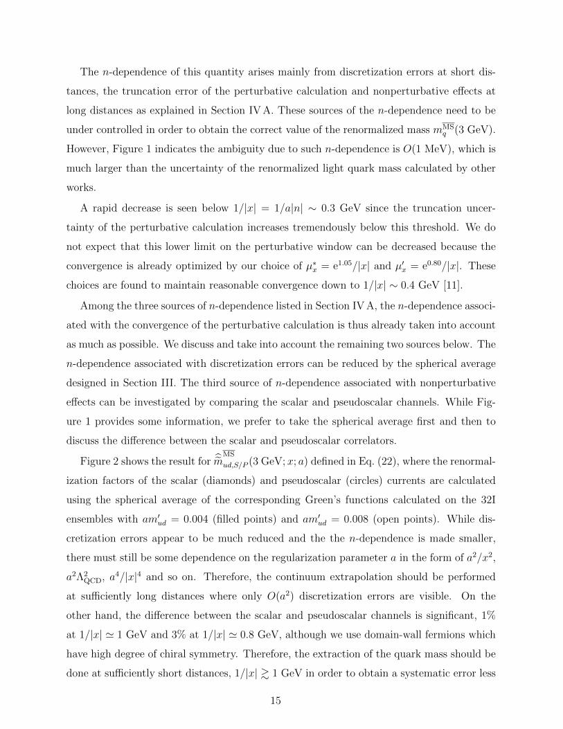
Figure 2 shows the result for mMS

ud,S/P (3 GeV;x; a) defined in Eq. (22), where the renormal-

ization factors of the scalar (diamonds) and pseudoscalar (circles) currents are calculated

using the spherical average of the corresponding Green’s functions calculated on the 32I

ensembles with am′ud = 0.004 (filled points) and am′ud = 0.008 (open points). While dis-

cretization errors appear to be much reduced and the the n-dependence is made smaller,

there must still be some dependence on the regularization parameter a in the form of a2/x2,

a2Λ2QCD, a4/|x|4 and so on. Therefore, the continuum extrapolation should be performed

at sufficiently long distances where only O(a2) discretization errors are visible. On the

other hand, the difference between the scalar and pseudoscalar channels is significant, 1%

at 1/|x| ' 1 GeV and 3% at 1/|x| ' 0.8 GeV, although we use domain-wall fermions which

have high degree of chiral symmetry. Therefore, the extraction of the quark mass should be

done at sufficiently short distances, 1/|x| & 1 GeV in order to obtain a systematic error less

15

���

���

���

���

���

���� ���� ���� ���� �� ���������������

���

������

���

�����������

������ ���������

〜�

�

�

��������������������������������

��������������������������������

���

���

���

���

���

���� ���� ���� ���� �� ����

FIG. 2. Results for mMS

ud,S/P (3 GeV; |x|; a,m′ud) calculated on the 32I ensembles.

than 1%. For this, the continuum extrapolation has to be safe at 1/|x| ' 1 GeV.

An important advantage of the spherical average is our ability to take the continuum

limit of renormalized quantities as explained below. Since the structure of the a-dependence

depends on |x| as it contains a term proportional to a2/x2, the renormalized quantities

need to be calculated at the same physical distance scale |x| for each ensemble in order

to take the continuum limit as a quadratic a2 → 0 extrapolation. The spherical averaging

technique trivially enables such an extrapolation. The extrapolation of the spherical averagemMS

ud,S/P (3 GeV; |x|; a,m′ud) to the continuum (a → 0) and chiral (m′ud → 0) limits is done

by performing a simultaneous fit to the data from all the ensembles with the fit function

mMS

ud,S/P (3 GeV; |x|; a,m′ud) = mMS

ud,S/P (3 GeV; |x|) + Ca,S/P (|x|)a2 + Cm,S/P (|x|)Mπ(a,m′ud)2,

(28)

with three fit parameters: mMS

ud,S/P (3 GeV; |x|), Ca,S/P (|x|) and Cm,S/P (|x|) for each |x|.

Here, we introduce a term proportional to the pion mass squared Mπ(a,m′ud)2 labeled by the

ensemble parameters a and m′ud, although the leading mass correction in perturbation theory

is proportional to quark mass squared or Mπ(a,m′ud)4. This is because the perturbative mass

correction is much smaller than the mass correction from OPE such as m〈qq〉 and m〈qGq〉

around 1/|x| ∼ 0.5 GeV [17, 26].

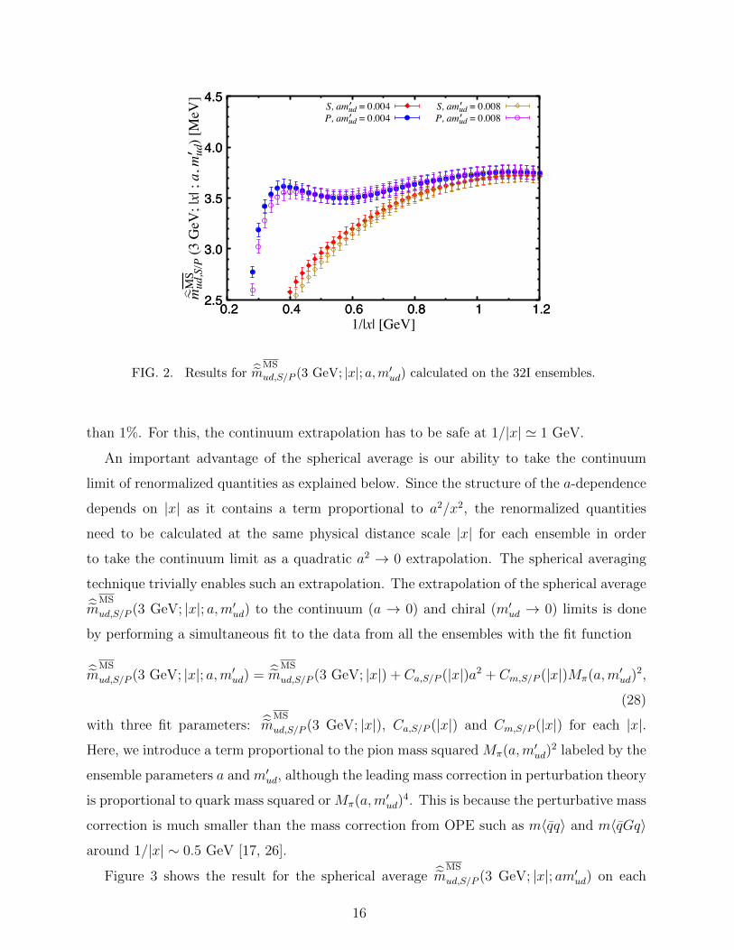
Figure 3 shows the result for the spherical average mMS

ud,S/P (3 GeV; |x|; am′ud) on each

16

���

���

���

���

���

���� ���� ���� ���� ���� ���� ���� ���������������

���

������

�����������

������ ���������

〜�

�

�

�����������������������������������

����������������������������������

����������������������������������������������������������������������������

���

���

���

���

���

���� ���� ���� ���� ���� ���� ���� ����

���

���

���

���

���

���� ���� ���� ���� ���� ���� ���� ���������������

���

������

�����������

���

��� ���������

〜�

�

�

�����������������������������������

����������������������������������

����������������������������������������������������������������������������

���

���

���

���

���

���� ���� ���� ���� ���� ���� ���� ����

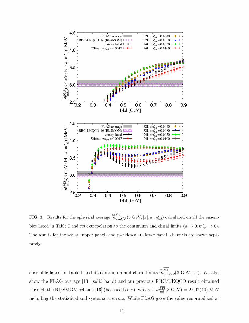
FIG. 3. Results for the spherical average mMS

ud,S/P (3 GeV; |x|; a,m′ud) calculated on all the ensem-

bles listed in Table I and its extrapolation to the continuum and chiral limits (a → 0,m′ud → 0).

The results for the scalar (upper panel) and pseudoscalar (lower panel) channels are shown sepa-

rately.

ensemble listed in Table I and its continuum and chiral limits mMS

ud,S/P (3 GeV; |x|). We also

show the FLAG average [13] (solid band) and our previous RBC/UKQCD result obtained

through the RI/SMOM scheme [16] (hatched band), which is mMSud (3 GeV) = 2.997(49) MeV

including the statistical and systematic errors. While FLAG gave the value renormalized at

17

���

���

���

���

���

���� ���� ���� ���� �� ���������������

���

������

�����������

������ ���������

〜�

�

�

�����������������������������������

������������

������������������������������������������������������������

���

���

���

���

���

���� ���� ���� ���� �� ����

���

���

���

���

���

���� ���� ���� ���� �� ���������������

���

������

�����������

���

��� ���������

〜�

�

�

�����������������������������������

������������

������������������������������������������������������������

���

���

���

���

���

���� ���� ���� ���� �� ����

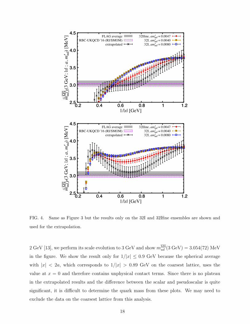
FIG. 4. Same as Figure 3 but the results only on the 32I and 32Ifine ensembles are shown and

used for the extrapolation.

2 GeV [13], we perform its scale evolution to 3 GeV and show mMSud (3 GeV) = 3.054(72) MeV

in the figure. We show the result only for 1/|x| ≤ 0.9 GeV because the spherical average

with |x| < 2a, which corresponds to 1/|x| > 0.89 GeV on the coarsest lattice, uses the

value at x = 0 and therefore contains unphysical contact terms. Since there is no plateau

in the extrapolated results and the difference between the scalar and pseudoscalar is quite

significant, it is difficult to determine the quark mass from these plots. We may need to

exclude the data on the coarsest lattice from this analysis.

18

Figure 4 shows the results on the finer two lattices (32I and 32Ifine). The continuum limit

is taken only with these lattice data, excluding the result on the coarsest ensembles. Since

the number of free parameters in Eq. (28) and the number of data points in this extrapolation

are both three, the extrapolation is not an actual χ2 fit but the free parameters can still be

determined, with propagated errors, by solving Eq. (28). While the |x|-dependence of the

extrapolated result becomes milder especially around 1/|x| ' 0.8 GeV, the statistical error

is substantially increased by discarding the data on the coarsest lattice. In order to obtain

a reasonable result with sufficiently small statistical error from such an analysis, we need to

introduce finer lattices.

Since it is currently not easy to introduce a finer lattice, we seek a more economical

analysis that enables to extract the quark mass from the data we currently have. Among

the three sources of the n-dependence of ZMS/latS/P (µ, 1/a; an;m′ud) mentioned in Section IV A,

we now focus on the third one, the nonperturbative effects. The nonperturbative effects on

the scalar and pseudoscalar correlators are known to be quite large compared to those on

the vector and axial-vector correlators in a model based on instantons because the scalar

and pseudoscalar channels are directly affected by instantons [27, 28]. The effect of a single

instanton on these channels, which is the most significant at short distances, is of the same

magnitude but with opposite sign [29]. Therefore, the naıve average of these two channels

may be free from the largest source of nonperturbative effects. Therefore, we analyze

mMS

q (3 GeV; |x|; a,m′ud) =mbareq (1/a)

ZMS/lat

S+P (3 GeV, 1/a; |x|;m′ud), (29)

with the O(4)-symmetric renormalization factorZ

MS/lat

S+P (3 GeV, 1/a; |x|;m′ud) obtained from

Eqs. (19) and (20) by substituting S/P with S + P and defining GlatS+P (1/a; |x|) as the

spherical average of the average of the scalar and pseudoscalar correlators.

Figure 5 shows the results for mMS

ud (3 GeV; |x|; a,m′ud). The continuum and chiral limits

are taken using the fit function

mMS

ud (3 GeV; |x|; a,m′ud) = mMS

ud (3 GeV; |x|) + Ca(|x|)a2 + Cm(|x|)Mπ(a,m′ud)2, (30)

with the fit parameters mMS

ud (3 GeV; |x|), Ca(|x|) and Cm(|x|). The fit results with (upper

panel) and without (lower panel) the data on the coarsest lattice are shown. We see a plateau

of the extrapolated data in the interval 0.4 GeV . 1/|x| . 0.6 GeV in the upper panel and

19

���

���

���

���

���

���� ���� ���� ���� ���� ���� ���� ���������������

�������

�����������

���

��� ���������

〜�

�

�

�����������������������������������

����������������������������������

����������������������������������������������������������������������������

���

���

���

���

���

���� ���� ���� ���� ���� ���� ���� ����

���

���

���

���

���

���� ���� ���� ���� �� ���������������

�������

�����������

���

��� ���������

〜�

�

�

�����������������������������������

������������

������������������������������������������������������������

���

���

���

���

���

���� ���� ���� ���� �� ����

FIG. 5. Results for the spherical average mMS

ud (3 GeV; |x|; a,m′ud) calculated from the average of

the scalar and pseudoscalar correlators. The results for the extrapolation to the continuum and

chiral limits (a→ 0,m′ud → 0) performed using all the ensembles (upper panel) and only the finer

two lattices (lower panel) are also shown.

0.4 GeV . 1/|x| . 0.8 GeV in the lower panel. These facts agree with the instanton-based

observation that the nonperturbative effects on the average of the scalar and pseudoscalar

correlators are much smaller than those on the individual channels.

Figure 6 shows the result for the strange quark mass defined in Eq. (29) with q = s, where

the same renormalization factors as for the light quark mass are used. The continuum and

20

��

��

���

���

���� ���� ���� ���� ���� ���� ���� ���������������

������

�����������

���

��� ���������

〜�

�

�

�����������������������������������

����������������������������������

����������������������������������������������������������������������������

��

��

���

���

���� ���� ���� ���� ���� ���� ���� ����

FIG. 6. Same as the upper panel of Figure 5 but the result for the strange quark mass.

���

���

���

���

���

���� ���� ���� ���� ���� ���� ���� ���������������

�����������

�

�

�������������������������

���

���

���

���

���

���� ���� ���� ���� ���� ���� ���� ����

FIG. 7. The χ2/d.o.f. obtained through the fit in the upper panel of Figure 5 (crosses) and in

Figure 6 (circles).

chiral extrapolations are done by the fit function (30) with the substitution mMS

ud → mMS

s .

A plateau is seen in the same region as in the result for the light quarks mass.

Figure 7 shows the χ2/d.o.f. obtained through the simultaneous fit both for the light

(crosses) and strange (circles) quark masses. While the position-space renormalization fac-

21

���

���

���

���

���

�� ����� ���� ����� ���� ����� ��������������

�������

�����������

������ ��

��

���������

〜�

�

�

�������������������

��������������������������������������������������������������������������������������������������

���

���

���

���

���

�� ����� ���� ����� ���� ����� ����

���

���

���

���

���

���

�� ����� ���� ����� ��������������

�������

�����������

����

���

��� ���������

〜�

�

�

�������������������

��������������������������������������������������������������������������������������������������

���

���

���

���

���

���

�� ����� ���� ����� ����

FIG. 8. Continuum and chiral extrapolations seen on the planes with Mπ = 0 (upper panel) and

a = 0 (lower panel) at 1/|x| = 0.52 GeV.

tors calculated on each ensemble are uncorrelated, the statistical errors for Zq and mbare,32Iq ,

which are taken from Ref. [16] and used in Eq. (26) to calculate unrenormalized quark mass

mbareq (1/a) for each lattice cutoff, are likely correlated. We interpret the small values of

χ2/d.o.f. shown in Figure 6 as resulting from our ignorance of such correlations. Since

χ2/d.o.f. at 1/|x| ' 0.6 GeV, which roughly corresponds to |x| ' 3a on the coarsest ensem-

ble, is not too large, we may conclude that the spherical average does not suffer significantly

from higher orders of O(a) errors for |x| & 3a.

22

To investigate the a- and Mπ-dependences of mMS

ud (3 GeV; |x|; a,m′ud) more clearly, we

visualize this extrapolation by analyzing the renormalized mass at a specific distance |x| in

the chiral limit

mMS

ud (3 GeV; |x|; a,m′ud → 0) ≡ mMS

ud (3 GeV; |x|; a,m′ud)− CmMπ(a,m′ud)2

= mMS

ud (3 GeV; |x|) + Caa2, (31)

and in the continuum limit

mMS

ud (3 GeV; |x|; a→ 0,m′ud) ≡ mMS

ud (3 GeV; |x|; a,m′ud)− Caa2

= mMS

ud (3 GeV; |x|) + CmMπ(a,m′ud)2, (32)

with the parameters mMS

ud (3 GeV; |x|), Ca(|x|) and Cm(|x|) obtained through the simultane-

ous fit Eq. (30). Figure 8 shows the result for these values with the lines of the extrapolation

at 1/|x| = 0.52 GeV. The result indicates both of the a- and Mπ-dependences are treated

well with their quadratic terms.

We use the result from the extrapolation including the data on the coarsest lattice to

determine the renormalized quark mass. We estimate the central value of the quark mass

at 1/|x| = 0.52 GeV, where χ2/d.o.f is minimum. Our result is

mMSud (3 GeV) = 3.113(36)(52)(24)(70) MeV. (33)

The first error is the statistical error. The second error is the systematic error due to

discretization effects, which is estimated by increasing 1/|x| up to 0.60 GeV where a deviation

from the plateau is beginning. The third error is the systematic uncertainty due to the

truncation of the perturbative calculation, which is estimated by varying the parameter µ∗x

in the region µ∗,optx /√

2 ≤ µ∗x ≤√

2µ∗,optx . The forth error corresponds to the systematic

error due to the uncertainty of the strong coupling constant, which is estimated by varying

the scale of three-flavor QCD in the region 315 MeV ≤ ΛMSQCD ≤ 349 MeV [18]. The result

is compatible with our previous RBC/UKQCD result mMSud (3 GeV) = 2.997(49) MeV [16]

obtained through the RI/SMOM scheme using the same lattice ensembles and with the

FLAG average mMSud (3 GeV) = 3.054(72) MeV [13] of many works done through various

renormalization procedures including the RI/(S)MOM and the Schrodinger functional [30]

methods using 2 + 1-flavor ensembles. Applying the same procedure, we obtain the strange

23

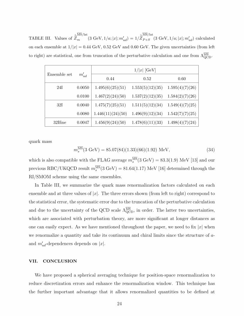
TABLE III. Values ofˆZ

MS/lat

m (3 GeV, 1/a; |x|;m′ud) = 1/ˆZ

MS/lat

P+S (3 GeV, 1/a; |x|;m′ud) calculated

on each ensemble at 1/|x| = 0.44 GeV, 0.52 GeV and 0.60 GeV. The given uncertainties (from left

to right) are statistical, one from truncation of the perturbative calculation and one from ΛMSQCD.

Ensemble set m′ud

1/|x| [GeV]

0.44 0.52 0.60

24I 0.0050 1.495(6)(25)(51) 1.553(5)(12)(35) 1.595(4)(7)(26)

0.0100 1.467(2)(24)(50) 1.537(2)(12)(35) 1.584(2)(7)(26)

32I 0.0040 1.475(7)(25)(51) 1.511(5)(12)(34) 1.549(4)(7)(25)

0.0080 1.446(11)(24)(50) 1.496(9)(12)(34) 1.542(7)(7)(25)

32Ifine 0.0047 1.456(9)(24)(50) 1.478(6)(11)(33) 1.498(4)(7)(24)

quark mass

mMSs (3 GeV) = 85.07(84)(1.33)(66)(1.92) MeV, (34)

which is also compatible with the FLAG average mMSs (3 GeV) = 83.3(1.9) MeV [13] and our

previous RBC/UKQCD result mMSs (3 GeV) = 81.64(1.17) MeV [16] determined through the

RI/SMOM scheme using the same ensembles.

In Table III, we summarize the quark mass renormalization factors calculated on each

ensemble and at three values of |x|. The three errors shown (from left to right) correspond to

the statistical error, the systematic error due to the truncation of the perturbative calculation

and due to the uncertainty of the QCD scale ΛMSQCD, in order. The latter two uncertainties,

which are associated with perturbation theory, are more significant at longer distances as

one can easily expect. As we have mentioned throughout the paper, we need to fix |x| when

we renormalize a quantity and take its continuum and chiral limits since the structure of a-

and m′ud-dependences depends on |x|.

VII. CONCLUSION

We have proposed a spherical averaging technique for position-space renormalization to

reduce discretization errors and enhance the renormalization window. This technique has

the further important advantage that it allows renormalized quantities to be defined at

24

any fixed physical distance. This allows a direct matching between renormalized quantities

defined on ensembles with different lattice spacings and a continuum limit to be easily taken

for position-space renormalized quantities at a fixed, physical renormalization scale.

The technique is applied to the quark mass renormalization using the scalar and pseu-

doscalar correlators in position space. We investigate the |x|-dependence of the renormalized

quark mass in the continuum limit and find a plateau even when the MS renormalized quark

mass at finite a still depends slightly on the distance |x| at which the intermediate position-

space scheme is applied. The investigation of the χ2/d.o.f. found for the continuum and

chiral extrapolations implies that the a-dependence of sphere-averaged correlator is mostly

O(a2) in the region |x| & 3a. The renormalized quark mass obtained through this renor-

malization procedure agrees with the FLAG average and our previous RBC/UKQCD result

obtained by using the RI/SMOM renormalization scheme on the same lattice ensembles.

The averaging approach proposed here is one of many possible schemes that can be

devised which involve a smearing or averaging over lattice points in position space. However,

the scheme proposed here may be of particular value because it involves two quite sharply

defined scales: a long-distance scale |x|, the radius of the sphere over which we average, and

a short-distance scale, the lattice spacing a which describes the thickness of the spherical

shell of points which are averaged. The multi-linear interpolation method which is employed

might be viewed as among the simplest prescriptions for creating this average. Having two

such distinct scales may improve the continuum limit of the quantities renormalized using

this method.

Since this X-space scheme is gauge invariant and free from contact terms, it prevents the

mixing with irrelevant operators, which can be a serious complication for gauge-noninvariant

schemes such as the RI/MOM scheme. Therefore, this position-space renormalization is

especially well-suited for the four-quark operators in the ∆S = 1 weak Hamiltonian where

it can be imposed at the relatively long distances needed to define three-flavor operators —

distances much longer than the Compton wavelength of the charm quark. At such distances

(or at the corresponding energies below 1 GeV), the RI/MOM scheme is plagued by gauge

noise and the usually justified neglect in the RI/MOM scheme of additional dimension-six

operators constructed from a product of quark bilinears and gluon fields is likely to be a

poor approximation. In fact, one of the motivations for this X-space method is to allow

the Wilson coefficients of the three-flavor ∆S = 1 weak Hamiltonian to be determined non-

25

perturbatively in terms of the more accurate, perturbatively-determined Wilson coefficients

of the corresponding four-flavor theory.

Further technique must be developed before such a complete three-to-four flavor matching

is possible. Some renormalization conditions can be imposed on the position-space two-point

functions of four-quark operators renormalized in analogy with the sphere average of the

two-point functions of scalar or pseudo-scalar currents presented in this paper. However,

such in a position-space scheme, we will also need to constrain other Green’s functions such

as three-point functions of a four-quark operator and two two-quark operators to uniquely

define a position-space scheme. The two-point functions of N mixing operators, will form

a real symmetric matrix and allow at most N(N + 1)/2 renormalization conditions to be

imposed. These will be insufficient to determine the needed N ×N renormalization matrix.

An extension of the spherical averaging procedure to such three-point functions is the next

step with is being developed.

ACKNOWLEDGMENTS

The authors thank their RBC and UKQCD colleagues for many useful discussions espe-

cially Peter Boyle and Robert Mawhinney. This work is supported in part by the US DOE

grant #de-sc0011941.

Appendix A: Irregular a-dependence of spherical average

Since the interpolation Eq. (14) contains nµ = bxµ/ac, which is a discontinuous function

of x/a, some irregularity could occur and the continuum extrapolation with only a term

proportional to a2 may not be accurate. In this Appendix, we discuss the significance of

such irregular a-dependence of the spherical average.

Let us begin with the case of one dimension, in which the interpolated value f(x) of a

quantity f(x) defined in Eq. (10) can be written as

fa(x) = F (x) + ca(x)a2 +x2F ′′(x)

2

(ax

(n+ 1)− 1)(

1− a

xn)

+O(a3). (A1)

Here, F ′′(x) stands for the second derivative of F (x) and ca(x) comes from ca,n and ca,n+1

in Eq. (9), which are the discretization errors in the values fa,n and fa,n+1 evaluated on the

lattice. We omit the possible logarithmic a-dependence of F (x) and F ′′(x) for simplicity.

26

�����

�����

�����

����

����

����

����

�� ���� ���� ���� ���� ���� ���������

�������

���������������������

�

�

�

���������������

����������

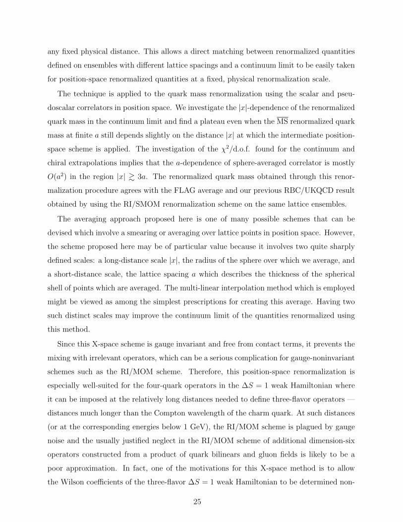
FIG. 9. B1(x; a)/(x2F ′′(x)), B2(|x|; a)/(x2Frr(|x|)) and B4(|x|; a)/(x2Frr(|x|)) plotted as func-

tions of a/|x|. The curve of (a/|x|)2/8 is also plotted for comparison.

While the both of the second and third terms in Eq. (A1) are expected to contain com-

plicated a-dependence, the third term

B1(x; a) =x2F ′′(x)

2

(ax

(n+ 1)− 1)(

1− a

xn), (A2)

can be explicitly analyzed and therefore is discussed first. Since the value of n = bx/ac

jumps where x/a is an integer, the a-dependence of I1(x; a)/(x2F ′′(x)) given by Eq. (A2)

is drawn (dashed curve) in Figure 9. Thus, the continuum extrapolation with a few data

points with an assumption of simple a2 discretization error could be inaccurate. While such

ambiguity is expected to be less than 1% of x2F ′′(x) in the case of one dimension, one

could imagine that in higher dimensions the spherical average further softens such irregular

dependence on a and makes the continuum extrapolation more accurate.

The interpolation in d dimensions can be written as

fa(x) = F (x) + ca(x)a2 +Bd(x; a) +O(a3), (A3)

where

Bd(x; a) =x2

2

d∑µ=1

Fµµ(x)

(a

|x|(nµ + 1)− xµ

|x|

)(xµ|x|− a

|x|nµ

), (A4)

and Fµµ(x) is the second derivative of F (x) with respect to xµ. Averaging over the sphere

by the integral given in Eq. (12) for two dimensions or in Eq. (16) for four dimensions, this

27

�����

�����

�����

����

����

����

����

�� ���� ���� ���� ���� ���� ���������

���

����

����������� ����������

�����

�

�

�

����������

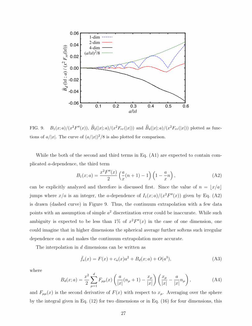
FIG. 10. B2(|x|; a)/(a2Frr(|x|)) and B4(|x|; a)/(a2Frr(r)) shifted by δd, the mid point of the

oscillation. Note by dividing by a2 instead of by |x|2 as is done in Figure 9, we are plotting the

correction relative to the regular a2 error.

term becomes

Bd(|x|; a) = Cd x2

∫ π/2

0

dθ sind−2 θ

(Frr(|x|) cos2 θ +

Fr(|x|)|x|

sin2 θ

)×(a

|x|

(⌊|x|a

cos θ

⌋+ 1

)− cos θ

)(cos θ − a

|x|

⌊|x|a

cos θ

⌋), (A5)

where

C2 =2

π, C4 =

8

π, (A6)

and Fr(|x|) and Frr(|x|) respectively stand for the first and second derivatives of F (|x|) with

respect to |x|.

In order to describe the a dependence implied by Eq. (A5), we need to assume a relation

between the Frr(|x|) and Fr(|x|)/|x| terms found in the first line of that equation. For the

purposes of illustration we will assume that F (|x|), which in this application is expected

to be a slowly varying function of |x|, behaves as ln(|x|) so we can replace Fr(|x|) by the

|x|Frr(|x|). In this case, Eq. (A5) becomes

Bd(|x|; a) ' Cdx2Frr(|x|)

∫ π/2

0

dθ sind−2 θ(2 cos2 θ − 1

)×(a

|x|

(⌊|x|a

cos θ

⌋+ 1

)− cos θ

)(cos θ − a

|x|

⌊|x|a

cos θ

⌋). (A7)

28

������

������

������

�����

�� ����� ���� �������������

�������

������

�

�

�

�������������������������������������������������������

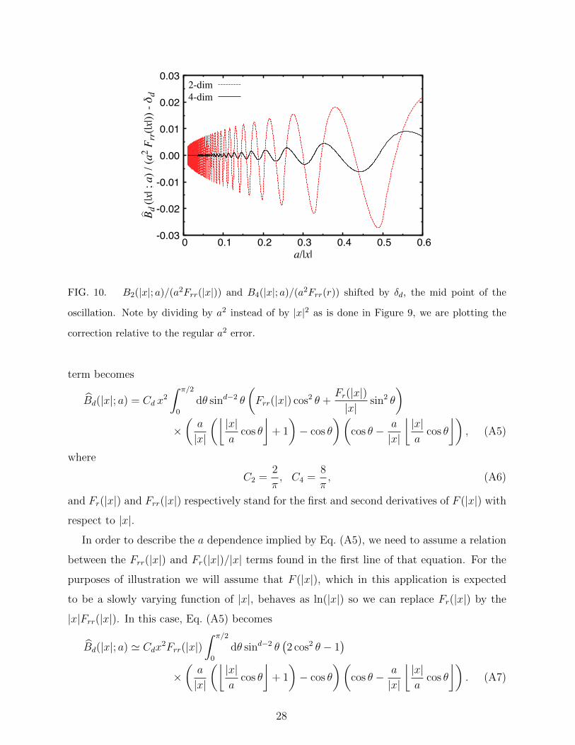
FIG. 11. ∆S(|x|;m2) versus (a/|x|)2 for several values of m|x|.

Figure 9 also shows the results for the spherical average Bd(|x|; a) normalized by x2Frr(|x|) in

two and four dimensions. The magnitude of the irregular a-dependence in two dimensions is

smaller than that in one dimension and therefore the continuum extrapolation with a regular

a2 term is expected to be more accurate. The irregular a-dependence of the spherical average

in four dimensions is even smaller than that in two dimensions in the sense explained below.

The significance of the irregular term in

Bd(|x|; a)

x2Frr(|x|)= δd · (a/|x|)2 + (irregular oscillation) +O

((a/|x|)3

), (A8)

can be investigated by

Bd(|x|; a)

a2Frr(|x|)− δd, (A9)

which is plotted in Figure 10 for two and four dimensions. Here, we find δ2 ' 0.00047 and

δ4 ' 0.16667. As the figure indicates, the irregular oscillation in four dimensions is even

smaller than that in two dimensions. It means the continuum limit can be safely taken with

a regular a2 term.

Thus, we conclude that the irregular a-dependence associated with the third term of

Eq. (A1) or (A3) is negligible. We proceed to discuss the other source of the irregular

29

a-dependence associated with ca(x) in Eq. (A1) or (A3), which can be written as

ca(x) = a−41∑

i,j,k,l=0

∆1,i∆2,j∆3,k∆4,l ca,n+i1+j2+k3+l4, (A10)

in the case of four dimensions. Here, cn for the scalar or pseudoscalar correlator may be

roughly approximated to a dispersion integral of the difference between the lattice and

continuum propagators of a scalar field

ca,na2 =

∫ ∞0

ds ρ(s)δDF (an; s), (A11)

δDF (an;m2) = DlatF (an;m2)−Dcont

F (an;m2), (A12)

DlatF (an;m2) =

∫ π/a

−π/a

d4q

(2π)4eiaqn

1

4a−2∑

µ sin2 aqµ2

+m2, (A13)

DcontF (x;m2) =

∫ ∞−∞

d4q

(2π)4eiqx

1

q2 +m2=

m

4π2

K1(m|x|)|x|

, (A14)

where ρ(s) is the corresponding spectral function and K1(z) is the modified Bessel function

of the second kind. To quantify the significance of cn, we analyze the spherical average

∆S(|x|;m2) of

∆S(an;m2) =δDF (an;m2)

DcontF (x;m2)

∣∣x=an

. (A15)

The result is shown in Figure 11, which indicates that the discretization error is mostly

proportional to a2 for |x| & 3a and that the continuum extrapolation using lattice data at

|x| ' 3a, 4a and 5a is likely accurate within the O(0.1%) level.

While the above analysis using the bosonic propagator may be valid in QCD at long

distances, the discretization error of Green’s functions in the perturbative regime may need to

be discussed in terms of fermionic propagators. We analyze the spherical average ∆2f (|x|; 0)

of

∆2f (an; 0) = limm→0

Glat,freeS (an;m)−Gcont,free

S (x;m)

Gcont,freeS (x;m)

∣∣∣∣∣x=an

, (A16)

Gcont,freeS (x;m) =

3

π4x6, (A17)

Glat,freeS (x;m) = Tr

[Slat,freeF (x;m)Slat,free

F (−x;m)], (A18)

where the lattice propagator Slat,freeF (an;m) in free field theory at small input mass am .

0.1 is quite sensitive to finite volume since the physical length scale in the deconfinement

phase is associated with the input quark mass, not the pion mass. Here, we calculate it

30

���

���

���

���

�� ����� ���� ����� ���� �������������

�������

�����

�

�

�

�����

����

����

����

����

�� ����� ����� ����� �����

���

���

���

���

�� ������ ������ ������ ��������������

�������

�����

�

�

�

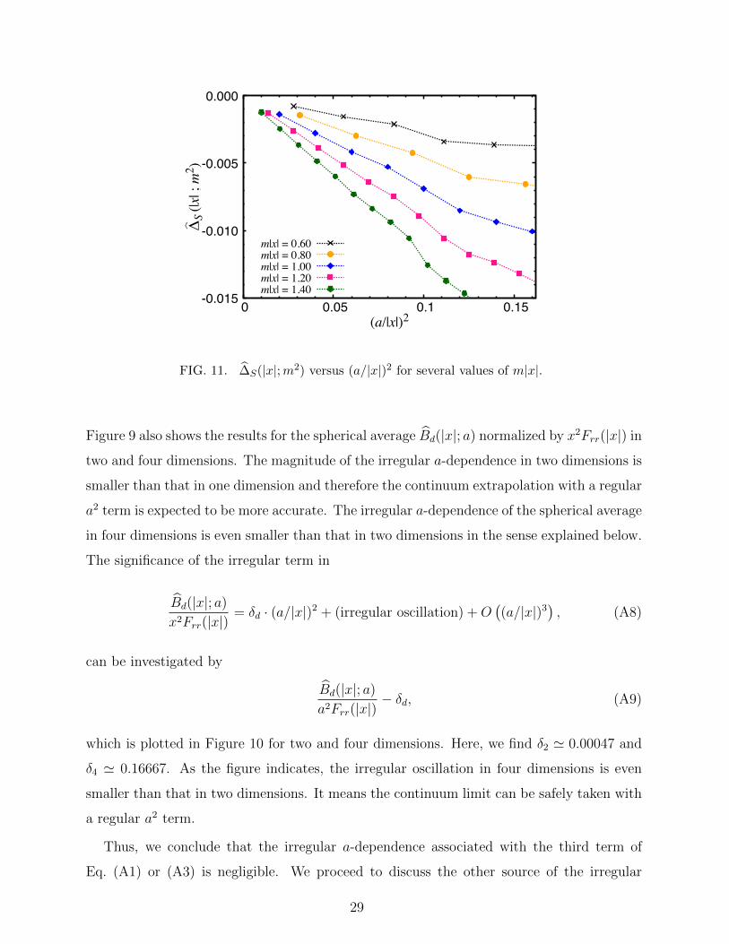
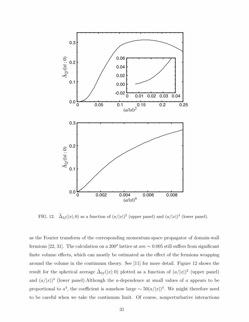
FIG. 12. ∆2f (|x|; 0) as a function of (a/|x|)2 (upper panel) and (a/|x|)4 (lower panel).

as the Fourier transform of the corresponding momentum-space propagator of domain-wall

fermions [22, 31]. The calculation on a 2004 lattice at am ∼ 0.005 still suffers from significant

finite volume effects, which can mostly be estimated as the effect of the fermions wrapping

around the volume in the continuum theory. See [11] for more detail. Figure 12 shows the

result for the spherical average ∆2f (|x|; 0) plotted as a function of (a/|x|)2 (upper panel)

and (a/|x|)4 (lower panel).Although the a-dependence at small values of a appears to be

proportional to a4, the coefficient is somehow large ∼ 50(a/|x|)4. We might therefore need

to be careful when we take the continuum limit. Of course, nonperturbative interactions

31

could reduce the magnitude of the O(a4) term to a size closer to that found above using the

bosonic propagator.

[1] G. Martinelli, G. C. Rossi, C. T. Sachrajda, S. R. Sharpe, M. Talevi, and M. Testa,

“Nonperturbative improvement of composite operators with Wilson fermions,” Phys. Lett.

B411 (1997) 141–151, arXiv:hep-lat/9705018 [hep-lat].

[2] V. Gimenez, L. Giusti, S. Guerriero, V. Lubicz, G. Martinelli, S. Petrarca, J. Reyes,

B. Taglienti, and E. Trevigne, “Non-perturbative renormalization of lattice operators in

coordinate space,” Phys. Lett. B598 (2004) 227–236, arXiv:hep-lat/0406019 [hep-lat].

[3] G. Martinelli, C. Pittori, C. T. Sachrajda, M. Testa, and A. Vladikas, “A General method

for nonperturbative renormalization of lattice operators,” Nucl. Phys. B445 (1995) 81–108,

arXiv:hep-lat/9411010 [hep-lat].

[4] M. Luscher, P. Weisz, and U. Wolff, “A Numerical method to compute the running coupling

in asymptotically free theories,” Nucl. Phys. B359 (1991) 221–243.

[5] K. Jansen, C. Liu, M. Luscher, H. Simma, S. Sint, R. Sommer, P. Weisz, and U. Wolff,

“Nonperturbative renormalization of lattice QCD at all scales,” Phys. Lett. B372 (1996)

275–282, arXiv:hep-lat/9512009 [hep-lat].

[6] RBC, UKQCD Collaboration, R. Arthur and P. A. Boyle, “Step Scaling with off-shell

renormalisation,” Phys. Rev. D83 (2011) 114511, arXiv:1006.0422 [hep-lat].

[7] K. Cichy, K. Jansen, and P. Korcyl, “Non-perturbative running of renormalization constants

from correlators in coordinate space using step scaling,” Nucl. Phys. B913 (2016) 278–300,

arXiv:1608.02481 [hep-lat].

[8] K. Symanzik, “Continuum Limit and Improved Action in Lattice Theories. 1. Principles and

phi**4 Theory,” Nucl. Phys. B226 (1983) 187–204.

[9] K. Symanzik, “Continuum Limit and Improved Action in Lattice Theories. 2. O(N)

Nonlinear Sigma Model in Perturbation Theory,” Nucl. Phys. B226 (1983) 205–227.

[10] K. Cichy, K. Jansen, and P. Korcyl, “Non-perturbative renormalization in coordinate space

for Nf = 2 maximally twisted mass fermions with tree-level Symanzik improved gauge

action,” Nucl. Phys. B865 (2012) 268–290, arXiv:1207.0628 [hep-lat].

[11] JLQCD Collaboration, M. Tomii, G. Cossu, B. Fahy, H. Fukaya, S. Hashimoto, T. Kaneko,

32

and J. Noaki, “Renormalization of domain-wall bilinear operators with short-distance

current correlators,” Phys. Rev. D94 no. 5, (2016) 054504, arXiv:1604.08702 [hep-lat].

[12] K. G. Chetyrkin and A. Maier, “Massless correlators of vector, scalar and tensor currents in

position space at orders α3s and α4

s: Explicit analytical results,” Nucl. Phys. B844 (2011)

266–288, arXiv:1010.1145 [hep-ph].

[13] S. Aoki et al., “Review of lattice results concerning low-energy particle physics,” Eur. Phys.

J. C77 no. 2, (2017) 112, arXiv:1607.00299 [hep-lat].

[14] Y. Aoki et al., “Non-perturbative renormalization of quark bilinear operators and B(K)

using domain wall fermions,” Phys. Rev. D78 (2008) 054510, arXiv:0712.1061 [hep-lat].

[15] C. Sturm, Y. Aoki, N. H. Christ, T. Izubuchi, C. T. C. Sachrajda, and A. Soni,

“Renormalization of quark bilinear operators in a momentum-subtraction scheme with a

nonexceptional subtraction point,” Phys. Rev. D80 (2009) 014501, arXiv:0901.2599

[hep-ph].

[16] RBC, UKQCD Collaboration, T. Blum et al., “Domain wall QCD with physical quark

masses,” Phys. Rev. D93 no. 7, (2016) 074505, arXiv:1411.7017 [hep-lat].

[17] M. C. Chu, J. M. Grandy, S. Huang, and J. W. Negele, “Correlation functions of hadron

currents in the QCD vacuum calculated in lattice QCD,” Phys. Rev. D48 (1993) 3340–3353,

arXiv:hep-lat/9306002 [hep-lat].

[18] ParticleDataGroup Collaboration, M. Tanabashi et al., “Review of Particle Physics,”

Phys. Rev. D98 no. 3, (2018) 030001.

[19] P. A. Baikov, K. G. Chetyrkin, and J. H. Kuhn, “Quark Mass and Field Anomalous

Dimensions to O(α5s),” JHEP 10 (2014) 76, arXiv:1402.6611 [hep-ph].

[20] P. A. Baikov, K. G. Chetyrkin, and J. H. Kuhn, “Five-Loop Running of the QCD coupling

constant,” Phys. Rev. Lett. 118 no. 8, (2017) 082002, arXiv:1606.08659 [hep-ph].

[21] D. B. Kaplan, “A Method for simulating chiral fermions on the lattice,” Phys. Lett. B288

(1992) 342–347, arXiv:hep-lat/9206013 [hep-lat].

[22] Y. Shamir, “Chiral fermions from lattice boundaries,” Nucl. Phys. B406 (1993) 90–106,

arXiv:hep-lat/9303005 [hep-lat].

[23] Y. Iwasaki and T. Yoshie, “Renormalization Group Improved Action for SU(3) Lattice

Gauge Theory and the String Tension,” Phys. Lett. 143B (1984) 449–452.

[24] Y. Iwasaki, “Renormalization Group Analysis of Lattice Theories and Improved Lattice

33

Action: Two-Dimensional Nonlinear O(N) Sigma Model,” Nucl. Phys. B258 (1985) 141–156.

[25] RBC, UKQCD Collaboration, Y. Aoki et al., “Continuum Limit Physics from 2+1 Flavor

Domain Wall QCD,” Phys. Rev. D83 (2011) 074508, arXiv:1011.0892 [hep-lat].

[26] UKQCD Collaboration, S. J. Hands, P. W. Stephenson, and A. McKerrell, “Point-to-point

hadron correlation functions using the Sheikholeslami-Wohlert action,” Phys. Rev. D51

(1995) 6394–6402, arXiv:hep-lat/9412065 [hep-lat].

[27] G. ’t Hooft, “Computation of the Quantum Effects Due to a Four-Dimensional

Pseudoparticle,” Phys. Rev. D14 (1976) 3432–3450. [Erratum: Phys. Rev.D18,2199(1978)].

[28] V. A. Novikov, M. A. Shifman, A. I. Vainshtein, and V. I. Zakharov, “Are All Hadrons

Alike?,” Nucl. Phys. B191 (1981) 301.

[29] E. V. Shuryak, “Correlation functions in the QCD vacuum,” Rev. Mod. Phys. 65 (1993)

1–46.

[30] M. Luscher, R. Narayanan, P. Weisz, and U. Wolff, “The Schrodinger functional: A

Renormalizable probe for nonAbelian gauge theories,” Nucl. Phys. B384 (1992) 168–228,

arXiv:hep-lat/9207009 [hep-lat].

[31] R. Narayanan and H. Neuberger, “Infinitely many regulator fields for chiral fermions,” Phys.

Lett. B302 (1993) 62–69, arXiv:hep-lat/9212019 [hep-lat].

34