MAS6012 1 Turn Over

PLEASE LEAVE THIS EXAM PAPER ON YOUR DESK. DO NOT REMOVE IT FROM THE HALL. Data Provided: Neaves Tables Graph Paper

SCHOOL OF MATHEMATICS AND STATISTICS MAS6012 Session 2011 2012 3 Hours

Medical Statistics, Sampling, Design

RESTRICTED OPEN BOOK EXAMINATION. Candidates may bring to the examination lecture notes and associated lecture material (but no textbooks) plus a calculator that conforms to University regulations. All answers will be marked but credit will be given for only the best FIVE answers. All questions carry equal marks. Total marks 100.

Registration number from U-Card (9 digits) to be completed by student

MAS6012

MAS6012 2 Continued

(This page is left blank)

MAS6012 3 Turn Over

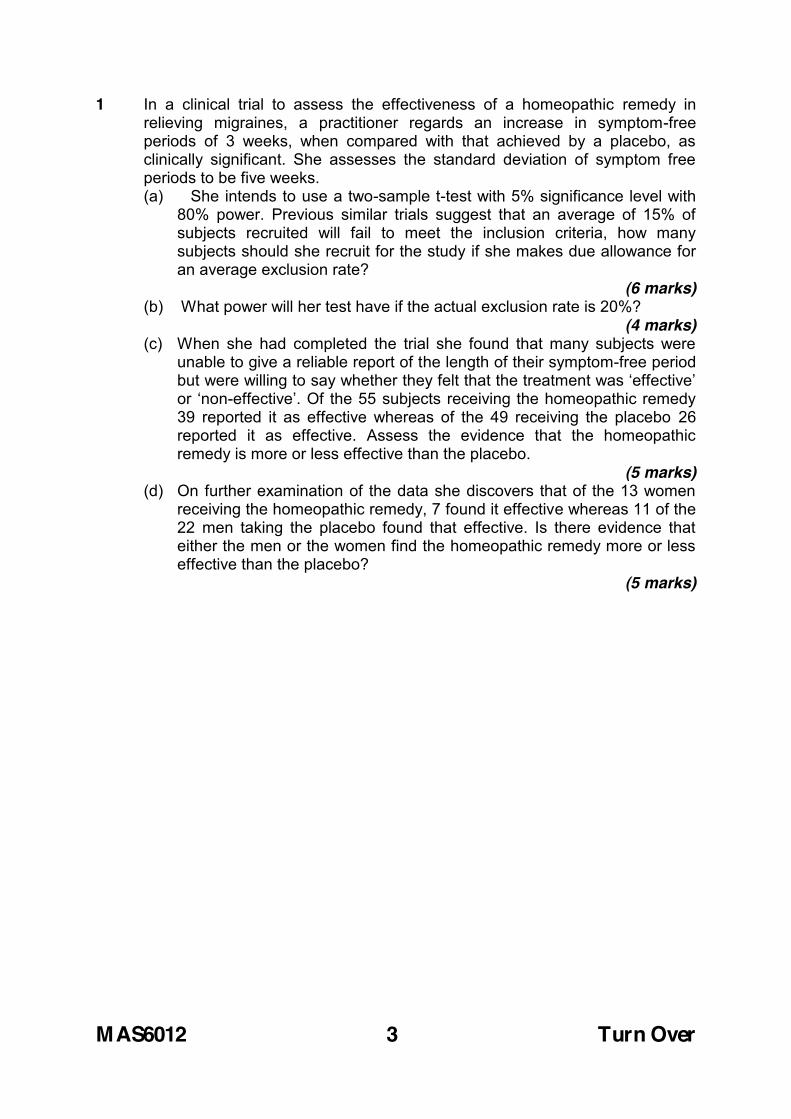
1 In a clinical trial to assess the effectiveness of a homeopathic remedy in relieving migraines, a practitioner regards an increase in symptom-free periods of 3 weeks, when compared with that achieved by a placebo, as clinically significant. She assesses the standard deviation of symptom free periods to be five weeks. (a) She intends to use a two-sample t-test with 5% significance level with

80% power. Previous similar trials suggest that an average of 15% of subjects recruited will fail to meet the inclusion criteria, how many subjects should she recruit for the study if she makes due allowance for an average exclusion rate?

(6 marks) (b) What power will her test have if the actual exclusion rate is 20%?

(4 marks) (c) When she had completed the trial she found that many subjects were

unable to give a reliable report of the length of their symptom-free period

-39 reported it as effective whereas of the 49 receiving the placebo 26 reported it as effective. Assess the evidence that the homeopathic remedy is more or less effective than the placebo.

(5 marks) (d) On further examination of the data she discovers that of the 13 women

receiving the homeopathic remedy, 7 found it effective whereas 11 of the 22 men taking the placebo found that effective. Is there evidence that either the men or the women find the homeopathic remedy more or less effective than the placebo?

(5 marks)

MAS6012

MAS6012 4 Continued

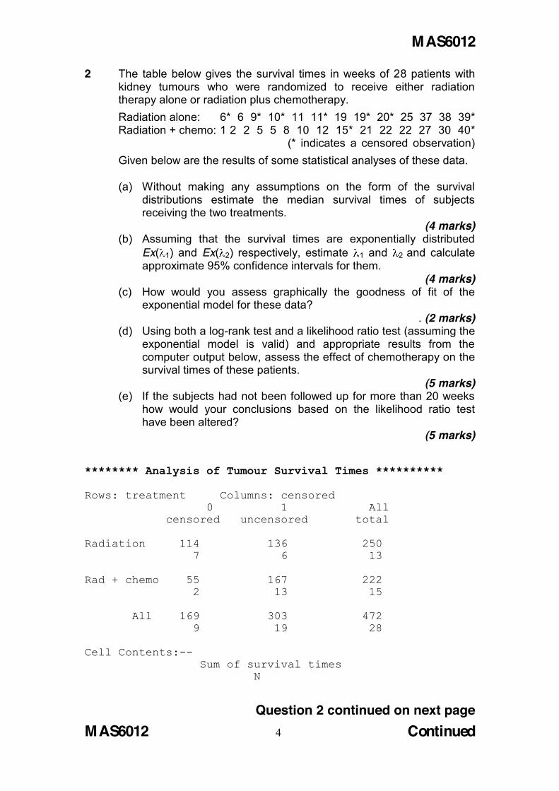
2 The table below gives the survival times in weeks of 28 patients with kidney tumours who were randomized to receive either radiation therapy alone or radiation plus chemotherapy.

Radiation alone: 6* 6 9* 10* 11 11* 19 19* 20* 25 37 38 39* Radiation + chemo: 1 2 2 5 5 8 10 12 15* 21 22 22 27 30 40* (* indicates a censored observation)

Given below are the results of some statistical analyses of these data.

(a) Without making any assumptions on the form of the survival distributions estimate the median survival times of subjects receiving the two treatments.

(4 marks) (b) Assuming that the survival times are exponentially distributed

Ex( 1) and Ex( 2) respectively, estimate 1 and 2 and calculate approximate 95% confidence intervals for them.

(4 marks) (c) How would you assess graphically the goodness of fit of the

exponential model for these data? . (2 marks)

(d) Using both a log-rank test and a likelihood ratio test (assuming the exponential model is valid) and appropriate results from the computer output below, assess the effect of chemotherapy on the survival times of these patients.

(5 marks) (e) If the subjects had not been followed up for more than 20 weeks

how would your conclusions based on the likelihood ratio test have been altered?

(5 marks)

 ********  Analysis  of  Tumour  Survival  Times  **********    Rows:  treatment          Columns:  censored                                      0                    1                        All                          censored      uncensored              total    Radiation          114                    136                      250                                  7                        6                        13    Rad  +  chemo        55                    167                      222                                  2                      13                        15                  All        169                    303                      472                                  9                      19                        28    Cell  Contents:-­-­                                                Sum  of  survival  times                                                    N  

     

Question 2 continued on next page

MAS6012

MAS6012 5 Turn Over

Question 2 continued   ***  Nonparametric  Survival  ***  Call:  survfit(formula  =  Surv(time,  censor,  type  =  "right")  ~  treatment,  type  =  "kaplan-­meier",  data  =  kidneytumour)    

                       n.obs  n.max  n.first  events  mean  se(mean)  median    treatment=1        13        13            13            6  28.3          3.79          37              treatment=2        15        15            15          13  15.6          3.11          12                

                               treatment=1      time  n.risk  n.event  survival  std.err  lower  95%  CI  upper  95%  CI            6          13              1        0.923    0.0739              0.7890                        1          9          11              0        0.923    0.0739              0.7890                        1        10          10              0        0.923    0.0739              0.7890                        1        11            9              1        0.821    0.1169              0.6206                        1        19            7              1        0.703    0.1477              0.4660                        1        20            5              0        0.703    0.1477              0.4660                        1        25            4              1        0.527    0.1883              0.2620                        1        37            3              1        0.352    0.1907              0.1215                        1        38            2              1        0.176    0.1567              0.0307                        1        39            1              0        0.176    0.1567              0.0307                        1    

                               treatment=2      time  n.risk  n.event  survival  std.err  lower  95%  CI  upper  95%  CI            1          15              1      0.9333    0.0644              0.8153                1.000          2          14              2      0.8000    0.1033              0.6212                1.000          5          12              2      0.6667    0.1217              0.4661                0.953          8          10              1      0.6000    0.1265              0.3969                0.907        10            9              1      0.5333    0.1288              0.3322                0.856        12            8              1      0.4667    0.1288              0.2717                0.802        15            7              0      0.4667    0.1288              0.2717                0.802        21            6              1      0.3889    0.1287              0.2033                0.744        22            5              2      0.2333    0.1150              0.0888                0.613        27            3              1      0.1556    0.0995              0.0444                0.545        30            2              1      0.0778    0.0742              0.0120                0.504        40            1              0      0.0778    0.0742              0.0120                0.504  

Time

Survival

0 10 20 30 40

0.0

0.2

0.4

0.6

0.8

1.0 treatment=1

treatment=2

Question 2 continued on next page

MAS6012

MAS6012 6 Continued

Question 2 continued survdiff(Surv(time,  censor)~treatment,data=kidneytumour)  Call:  survdiff(formula  =  Surv(time,  censor)  ~  treatment,  data  =       kidneytumour)                              N  Observed  Expected  (O-­E)^2/E    

treatment=1  13                6          9.99            ?????  treatment=2  15              13          9.01            ?????

 Chisq=  ?????    on  1  degrees  of  freedom,  p=  ?????  

MAS6012

MAS6012 7 Turn Over

3 Given below is a record (edited in places) of an R session analysing the results of a randomized double-blind two period crossover trial comparing nphenomenon. The data are the number of attacks in two weeks. Patients were randomly allocated to two groups: group 1 received treatment N in period 1 and P in period 2. Group 2 received the treatments in the opposite order. (a) Plot the treatment means for each period.

(3 marks) (b) Assess all of the evidence that there is a carryover effect from

period 1 to period 2. (5 marks)

(c) Do the data provide evidence that there is a difference in average response between periods 1 and 2?

(4 marks) (d) Assess whether the treatments differ in effect, taking into account

the results of your assessments of carryover and period effects. (5 marks)

(e) Which, if any, of the three confidence intervals provided in the analyses below provides a confidence interval for the effect of the treatment with nicardipine on the number of attacks in patients with

(3 marks)

Question 3 continued on next page

MAS6012

MAS6012 8 Continued

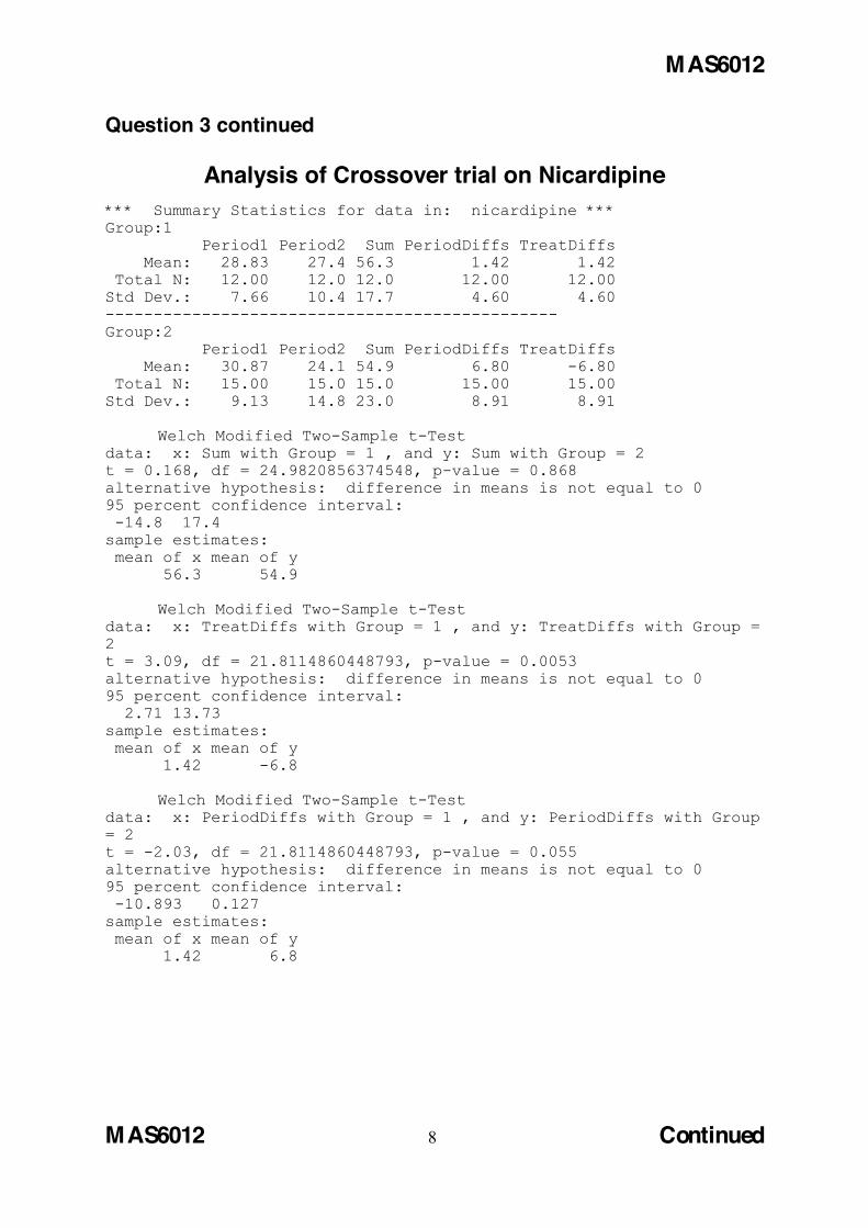
Question 3 continued

Analysis of Crossover trial on Nicardipine ***    Summary  Statistics  for  data  in:    nicardipine  ***  Group:1                      Period1  Period2    Sum  PeriodDiffs  TreatDiffs            Mean:      28.83        27.4  56.3                1.42              1.42    Total  N:      12.00        12.0  12.0              12.00            12.00  Std  Dev.:        7.66        10.4  17.7                4.60              4.60  -­-­-­-­-­-­-­-­-­-­-­-­-­-­-­-­-­-­-­-­-­-­-­-­-­-­-­-­-­-­-­-­-­-­-­-­-­-­-­-­-­-­-­-­-­-­-­  Group:2                      Period1  Period2    Sum  PeriodDiffs  TreatDiffs            Mean:      30.87        24.1  54.9                6.80            -­6.80    Total  N:      15.00        15.0  15.0              15.00            15.00  Std  Dev.:        9.13        14.8  23.0                8.91              8.91       Welch  Modified  Two-­Sample  t-­Test  data:    x:  Sum  with  Group  =  1  ,  and  y:  Sum  with  Group  =  2    t  =  0.168,  df  =  24.9820856374548,  p-­value  =  0.868    alternative  hypothesis:    difference  in  means  is  not  equal  to  0    95  percent  confidence  interval:    -­14.8    17.4    sample  estimates:    mean  of  x  mean  of  y                56.3            54.9       Welch  Modified  Two-­Sample  t-­Test  data:    x:  TreatDiffs  with  Group  =  1  ,  and  y:  TreatDiffs  with  Group  =  2    t  =  3.09,  df  =  21.8114860448793,  p-­value  =  0.0053    alternative  hypothesis:    difference  in  means  is  not  equal  to  0    95  percent  confidence  interval:      2.71  13.73    sample  estimates:    mean  of  x  mean  of  y                1.42            -­6.8       Welch  Modified  Two-­Sample  t-­Test  data:    x:  PeriodDiffs  with  Group  =  1  ,  and  y:  PeriodDiffs  with  Group  =  2    t  =  -­2.03,  df  =  21.8114860448793,  p-­value  =  0.055    alternative  hypothesis:    difference  in  means  is  not  equal  to  0    95  percent  confidence  interval:    -­10.893      0.127    sample  estimates:    mean  of  x  mean  of  y                1.42              6.8    

MAS6012

4 An investigator is studying the dependence of a variable Y on two continuousexplanatory variables x1 and x2, which have been scaled to lie between -1 and 1.It is known that EY = 0 when both x1 = 0 and x2 = 0, and the following modelis proposed. Each observation is subject to a measurement error with mean 0 andvariance σ2.

EY = β1x1 + β2x2.

The investigator proposes to take four observations, at (-1,0), (1,0), (0,-1) and(0,1). Denote the four observations by Y1, . . . , Y4.

(i) Find the least squares estimators of β1 and β2, verify that they are unbiased,and give their variances in terms of σ2 only. (5 marks)

(ii) By examining the form of your estimators in part (i) (rather than by con-sidering the design matrix), briefly explain why β1 and β2 are orthogonal toeach other for the chosen design. (2 marks)

(iii) Show that this design is neither D-optimal nor G-optimal, by using theGeneral Equivalence Theorem. (4 marks)

(iv) Suggest an alternative design, with four observations, that is D-optimal.Justify your suggestion. (6 marks)

(v) If the A-optimality criterion is to be used, is your design in part (iv) betterthan the original proposed design? Justify your answer. (3 marks)

MAS6012 9 Turn Over

MAS6012

5 An experiment is to be carried out to investigate the effect of three diets andthree drugs on blood pressure. Nine volunteers are recruited to the study, and aregrouped by weight into three blocks of three. A design is chosen based on thefollowing Latin square.

A B CC A BB C A

The following model is to be fitted to the data.

EYi j = µ+ θi + φj + ψκ(i ,j),

with i = 1, 2, 3 representing block, j = 1, 2, 3 representing diet, and ψκ(i ,j) repre-senting the effect of the drug given to the individual on diet j in block i (so thatκ(i , j) = 1, 2 or 3.) The constraints

3�

i=1

θi =3�

j=1

φj =3�

k=1

ψk = 0,

are applied.

(i) Write this model in matrix notation, and explain, with justification, whichgroups of parameters are orthogonal to each other. (7 marks)

(ii) Suppose the experiment is to be extended to investigate the effect of threedifferent exercise regimes, in addition to drug, diet and weight. State howyou would allocate exercise regimes to volunteers using a second Latinsquare that is orthogonal to the first. State how you would modify theoriginal model, and give the extra columns of the design matrix.

(7 marks)

(iii) In an alternative experiment, the effect of the three diets are to be consid-ered only, but volunteers will still be blocked by weight. If blocks of size twoare to be used, how many volunteers are required for the smallest possiblebalanced incomplete block design? For the smallest possible such design,list which diets should be used in each block. (3 marks)

If there are four diets to compare, can a balanced incomplete block designbe used with 8 blocks of size 3? Justify your answer. (3 marks)

MAS6012 10 Continued

MAS6012

6 (i) A small survey has been conducted to estimate the proportion of the pop-ulation in favour of raising the female retirement age. The sex of eachparticipant in the survey was recorded, and the results are given below.

males femalesin favour 23 15against 18 44

If the sample was drawn using simple random sampling, suggest two differ-ent estimates of the population proportion in favour of raising the femaleretirement age. Briefly explain your reasoning. (3 marks)

(ii) An opinion poll is to be taken to estimate the proportion of the adultpopulation in Scotland who are in favour of Scotland leaving the UnitedKingdom. If a simple random sample is to be used, how large would thesample need to be to ensure that a 90% confidence interval for the trueproportion was no wider than 0.1? You may ignore the finite populationcorrection. (5 marks)

(iii) 100 motors have various different ages, all of which are known. It is believedthat the remaining lifetime of each motor will be dependent on the motor’sage. Five motors are selected at random, their ages are noted and theirremaining lifetimes are observed by running them continuously until failure.Let Yi be the age of the i-th motor, and Xi be the remaining lifetime ofthe i-th motor. The following summary statistics are observed.

100�

i=1

Yi = 9024,5�

i=1

yi = 350,5�

i=1

xi = 4646,

5�

i=1

(xi − x)(yi − y) = −13754,5�

i=1

(yi − y)2 = 13960,

where (x1, y1), . . . , (x5, y5) are the observed age and remaining lifetime for5 randomly selected motors.

Suggest two possible estimates of X, explaining your reasoning. Withoutreferring explicitly to the formulae of your estimators, give an intuitiveexplanation for the discrepancy between the two estimates. (6 marks)

MAS6012 11 Question 6 continued on next page

MAS6012

6 (continued)

(iv) A survey is to be taken to estimate the mean starting wage of individualsfollowing completion of a new training course. Two pilot studies have beenconducted. In the first study, a simple random sample of size 20 was used,and the following summary statistics were observed.

20�

i=1

xi = 564.9,20�

i=1

x2i = 16131.2,

where each xi is measured in £1000.

In the second study, cluster sampling was used. Courses are run at differenttraining centres around the country, with 10 students at each centre. Twotraining centres were selected as the clusters. The following summarystatistics were observed.

10�

j=1

x1j = 258.7,10�

j=1

x21j = 6714.3,

10�

j=1

x2j = 305.0,10�

j=1

x22j = 9319.2,

where xi j is observation j within cluster i .

Based on the pilot survey data, would you recommend the use of clustersampling or simple random sampling for the new survey? Briefly explainyour reasoning. (6 marks)

End of Question Paper

MAS6012 12