MAS2317/3317: Introduction to Bayesian Statisticsnlf8/teaching/mas2317/notes/slides0.pdf · Dr. Lee...

MAS2317/3317:Introduction to Bayesian Statistics

Dr. Lee Fawcett

Semester 2, 2014—2015

Dr. Lee Fawcett MAS2317/3317: Introduction to Bayesian Statistics

Contact details

My name: Dr. Lee Fawcett

Office: Room 2.07 Herschel Building

Phone: 0191 208 7228

Email: [email protected]

www: www.mas.ncl.ac.uk/∼nlf8


Timetable and Administrative arrangements

Lectures are on Mondays at 11 (LT3) and Tuesdays at 12(LT2).

Problems classes are in ODD teaching weeks starting inteaching week 3. These take place on Thursdays at 9 inLT1. We will use this slot in week 1 as a lecture to getahead in the notes.

Drop–in sessions are at the same time and place inEVEN weeks starting in teaching week 4.

Computer practicals : Wednesdays at 12 (Herschel fullPC cluster). These happen in some EVEN weeks, and youwill be notified of these well in advance.


Timetable and Administrative arrangements

So to summarise:

Activity Day Time Room FrequencyLecture Mon 11–12 Herschel: LT3 Every week

Tues 12–1 Herschel: LT2 Every weekPC/ Thurs 9–10 Herschel: LT1 PC odd weeksDI DI even weeks

Practical Wed 12–1 Herschel: PC cluster Some even weeks


Assessment

Assessment is by:

End of semester exam in May/June (80%)

In course assessment, including written solution toproblems and computer practical work (10%)

Mid-semester test (10%)

No CBAs!

There will be four assignments, each one having a mixture ofwritten and practical questions.

Solutions to the starred questions should be submitted by thedates given in your notes.

We will work through the unstarred questions in problemsclasses and practicals.


Other stuff

Notes (with gaps) will be handed out in lectures – youshould fill in the gaps during lectures.

A summarised version of the notes will be used in lecturesas slides.

– Listen and learn– Write down– Announcements

These notes and slides will be posted on the coursewebsite and/or BlackBoard after each topic is finished,along with any other course material – such as problemssheets, model solutions to assignment questions,supplementary handouts etc.


Other stuff

The course website can be found via the “Additionalteaching information” link on the School’s webpage, ordirectly via:

http://www.mas.ncl.ac.uk/∼nlf8Please check your University email account regularly, ascourse announcements will often be made via email.

I have scheduled an office hour for this course (Fridaysfrom 1pm) where I will always be available to see studentswho need extra help/support with the course material.

I also have an office hour for MAS1343 (most Thursdays at3pm) that you are welcome to drop in to.


Preface to lecture notes:

The Bayesian paradigm


Statistics: an alternative approach

Up until now, you have been taught Probability andStatistics according to a particular way of thinking

The Bayesian paradigm offers another way of seeingthings

Your ideas about Probability and Statistics are deeplyentrenched...perhaps so much so that at first, BayesianStatistics might take you a while to grasp!

Not because it’s hard! Just because you have become soconditioned to think in a particular way!

I want to broaden your horizons a bit!


Bayes goes to war!

The work of Thomas Bayes (see later) was published in1764, 3 years after his death

Over the course of the next 100–150 years, it received littleattention

In fact, some key figures in Statistics – e.g. R.A. Fisher –outrightly rejected the idea of Bayesian statistics

By the start of WW2, Bayes’ rule was virtually taboo inthe world of Statistics!

During WW2, some of the world’s leading mathematiciansresurrected Bayes’ rule in deepest secrecy to crack thecoded messages of the Germans


Bayes goes to war!

Alan Turing – mathematician working at Bletchley Park

Designed the ‘bombe’ – an electro–mechanical machinefor testing every possible permutation of a messageproduced on the Enigma machine — could take up to 4days to decode a message

New system: Banburismus – where Bayesian methodswere used to quantify the belief in guesses of a stretch ofletters in an Enigma message

Certain permutations – unlikely to be the original message– were ‘thrown out’ before they were even tested

Greatly reduced the time it took to crack Enigma codes


Air France 447


Air France 447

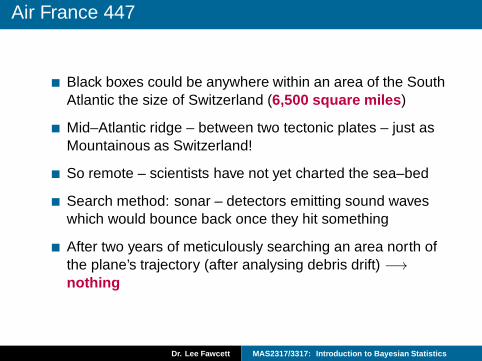
Black boxes could be anywhere within an area of the SouthAtlantic the size of Switzerland (6,500 square miles )

Mid–Atlantic ridge – between two tectonic plates – just asMountainous as Switzerland!

So remote – scientists have not yet charted the sea–bed

Search method: sonar – detectors emitting sound waveswhich would bounce back once they hit something

After two years of meticulously searching an area north ofthe plane’s trajectory (after analysing debris drift) −→nothing


Air France 447

April 2011: Metron, Inc., of Retson, Virginia, hired tolaunch a Bayesian review of the entire search effort

Included in the analysis were:

– Data from 9 previous airline crashes involving loss of pilotcontrol – reduced search area to 1,600 square miles

– Expert opinions on the credibility of the flight data

– Expert opinions about whether or not the black box‘pingers’ might have become damaged on impact

– Positions/recovery times of bodies found drifting – expertopinions assigned to the reliability of this data because ofthe turbulent equatorial waters

– Expert information from oceanographers: Sea state,visibility, underwater geography,...

All information combined through Bayes Theorem : Afterone week, black boxes found!


Motivating example

School A and School B each have a football team. They havetwo matches against each other coming up in the next fewweeks: a league match and a cup match.

What is the probability that School A wins both matches?


Equally likely outcomes?

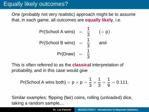
One (probably not very realistic) approach might be to assumethat, in each game, all outcomes are equally likely , i.e.

Pr(School A wins) =13

(= p)

Pr(School B wins) =13

and

Pr(Draw) =13

This is often referred to as the classical interpretation ofprobability, and in this case would give

Pr(School A wins both) = p × p =13× 1

3=

19= 0.111.

Similar examples: flipping (fair) coins, rolling (unloaded) dice,taking a random sample,...


Relative frequency approach?

Perhaps a better approach would be to consider what hashappened historically when these two teams have played eachother.

In fact, in their last 10 matches against each other, School Awon 7 times.

Then we might use

Pr(School A wins) =7

10(= p).

This is known as the relative frequency or frequentistinterpretation of probability, and would give

Pr(School A wins both) = p × p =7

10× 7

10=

49100

= 0.49.


Subjectivity?

You might argue that the second approach is more realistic.

However, you should notice that in both examples, once wehave figured out how likely it is that School A wins a matchagainst School B (p), this probability is assumed constant.

What if the team that wins the first match gains confidencebefore the second meeting?

What if they lost the last three consecutive matches?

What if School A think the cup match is more important?

What if we have some inside information: School A’s topscorer will be missing from one or both matches?

Enthusiastic supporters of School B might have their own(subjective) probabilities that their team will win, no matterwhat previous form suggests.


A third approach to probability

We have the classical approach to probability (equally likelyoutcomes).

We have the frequentist approach to probability (relativefrequency).

And then we have the subjective approach to probability.

When we work within the Bayesian framework, we try toaccount for subjective notions of probability, instead of(artificially) assuming equally likely outcomes or solely lookingat the outcomes of past ‘trials’ or ‘experiments’.


A third approach to probability

One way of doing this is to acknowledge that parameters in astatistical model (i.e. p in the above example) are not fixedconstants.

Perhaps it is okay to assume that our parameter of interest cantake on a whole range of values, reflecting the (perhapssubjective) beliefs of various parties?


Year 7 – The probability scale

I was introduced to the concept of probability in year 7.

We were asked to place a sunshine counter, a ten pence pieceand a Subbuteo figure on a ‘probability scale’ according to howlikely we thought the following events were to occur:

A: the sun will rise tomorrow;

B: I get a head when I flip a coin;

C: our school football team will win the cup this year.


“Results”


“Results”

Most of us understood there was an evens chance of getting ahead.

Most of us also believed the sun was certain to rise tomorrow,although you can see that one pupil has expressed some doubthere!

However, we all had different opinions about where to place thefootballer.

Pupil 2 was on the school football team

Most of us (thought we) knew our team were rubbish!

Pupil 6 had inside information!

A Bayesian analysis would take into account the variability ofthe pupils’ beliefs. The Probability and Statistics that you areused to would not do this.


Probability and Statistics at School

The National Curriculum probability syllabus steers clear ofevents like C – we were never told how to think aboutinterpreting subjective probabilities.

Teachers then have to focus on the Classical or frequentistinterpretations of probability – hence all those examples about

flipping (fair) coins

rolling (unloaded) dice

picking coloured balls at random from a bag

drawing cards from a pack

In short: pretty uninspiring!


Probability and Statistics at School

In fairness, you are taught about

the language of probability

correlation and regression

the Normal distribution

amongst other things, but let’s face it: most applications ofProbability and/or Statistics seem, at best, contrived, and nevertake into account subjectivity !


Probability and Statistics at University

First year: Not much better, but the aim of MAS1341/1342 is toget everyone up to the same level – basically A level standard.

You are introduced to Statistical inference : the process bywhich we attempt to infer things about the population based oninformation available in our sample.

Estimation

Confidence intervals

Hypothesis tests

All taught within the Classical /frequentist framework!


Example: Body Mass Index

Suppose we are interested in whether or not there is any realdifference between the Body Mass Index (BMI) of Maths &Stats students and Food & Human Nutrition students.

BMI is often used as a measure of ‘fatness’ or ‘thinness’: it isthe ratio of a person’s weight (measured in kg) to their squaredheight (measured in metres).

In a two–sample t–test, we often test the null hypothesis thatthere is no difference between the population means of the twogroups:

H0 : µM = µF ,

How can we test this hypothesis?



Suppose we obtain the following BMI values for a randomsample of students from both groups:

Maths & Stats 23.1 28.3 35.3 24.0 32.4 30.5 30.1 21.9 22.129.9 27.2 33.2

Food & Human Nutrition 25.5 27.3 21.0 23.3 19.1 22.2 29.5 27.5 23.2

From this we can obtain the summaries:

nM = 12 x̄M = 28.17 sM = 4.54

nF = 9 x̄F = 24.29 sF = 3.40



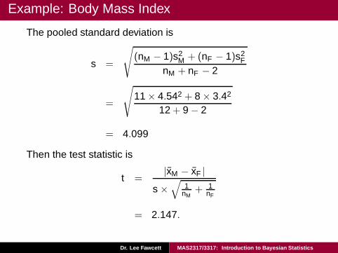
The pooled standard deviation is

s =

√

(nM − 1)s2M + (nF − 1)s2

F

nM + nF − 2

=

√

11 × 4.542 + 8 × 3.42

12 + 9 − 2

= 4.099

Then the test statistic is

t =|x̄M − x̄F |

s ×√

1nM

+ 1nF

= 2.147.



From t19–tables, we get:

p–value 10% 5% 1%critical value 1.729 2.093 2.861

Our test statistic t = 2.147 indicates that our p–value is lessthan 5%:

We have a significant result at the 5% level of significance

We reject H0

We conclude that there is a significant difference in BMIbetween M&S and FHN students



Notice from R that the exact p–value is 0.004488 = 4.488%.

As we have already concluded, we would reject H0 at the5% level;

However, if we work at the 1% level of significance, wewould retain H0!

What are we to do? Convention tells us to work at the 5% level,but why? Some practitioners work at the 1% level!



In MAS1341/1342 and MAS2304 you were introduced toBayes’ Theorem .

As we shall see, Bayes’ Theorem gives us a way of combiningsubjective assessments with observed data.

For example, what if – prior to observing the data – we believedthat Food & Human Nutrition students were likely to have aconsiderably lower BMI than Maths & Stats students?

What if, from a previous study, we knew that Maths & Statsstudents were quite likely to have a BMI somewhere between25 and 33?



Would it not be sensible to build this information into ouranalysis before forming our conclusions using the data alone?

This could be a good idea – we have relatively small samples,which could be biased!

A Bayesian analysis can do this!

Some people argue against this on the grounds that it issubjective... But as we have just seen, the usual approach tohypothesis testing is also subjective!

Not only are hypothesis tests tricky to interpret... but so areconfidence intervals .



Obtain a 95% confidence interval for the population mean BMIfor Maths & Stats students.

We usex̄M ± t

sM√nM

, giving

28.17 ± 2.201 × 4.54√12

i.e.

28.17 ± 2.743,

giving (25.28, 31.05).



What is Pr(25.28 < µM < 31.05)?

NOT 0.95!! In the frequentist approach, population parameters(in this case µM ) are NOT random variables!

This means µM is a fixed (but unknown) quantity. So it’s eitherin the interval, or it’s not, i.e.

Pr(25.28 < µM < 31.05) = 1 or

Pr(25.28 < µM < 31.05) = 0.

Nothing else!

Equivalent intervals in the Bayesian framework have morenatural interpretations!


Frequentist/Subjectivist debate

One of the main arguments against working within theBayesian paradigm is that it is subjective .

Although we have not yet thought about how the Bayesianframework combines subjective assessments with the data, wehave said that this is what it does.

Surely we should strive to be as objective as we can?



Actually, to be able to incorporate a person’s beliefs into ananalysis of sample data is surely the right thing to do —especially if that person is an expert!

This is in line with how scientific experiments are carried out:

The experimenter usually knows something ;

She then carries out the experiment in which data arecollected ;

the experimenter then updates her beliefs from theseresults.



In other words, the data are used to refine what theexperimenter knows.

And that is what MAS2317/3317 is all about – we will considerhow

prior beliefs can be combined with

experimental data to form

posterior beliefs – which include both the prior knowledgeand what we have learnt from the data


Bayesian Statistics: leading players

Thomas Bayes (1702–1761)

Presbyterian minister in Tunbridge Wells, Kent

Bayes’ solution to a problem of “inverse probability” waspresented in the Essay towards Solving a Problem in theDoctrine of Chances (1764)

Work published posthumously by his friend Richard Pricein the Philosophical Transactions of the Royal Society ofLondon.

This work gives us Bayes’ Theorem , a key result on whichmost of the work in this course rests.



Bruno di Finetti (1906–1985)

Italian mathematical probabilist, developed his ideas onsubjective probability in the 1920s.

Famed for saying

“Probability does not exist”

By this, he meant it has no objective existence – i.e. it isnot a feature of the world around us.

It is a measure of degree–of–belief – your belief, my belief,someone else’s belief – all of which could be different.



Dennis Lindley (1923—2013)

Worked hard to find a mathematical basis for the subject ofStatistics

With Leonard Savage, he found a deeper justification forStatistics in Bayesian theory

Turned into a critic of the classical statistical inference hehad hoped to justify

Quoted as saying:

“Uncertainty is a personal matter. It is not the uncertainty,but your uncertainty”


Recent developments

One of the difficulties in early applications of Bayesianmethodology was the maths:

Combining prior beliefs with a probability model for the dataoften resulted in maths that was just too difficult/impossibleto solve by hand .


Recent developments

Then – in the early 1990s – a technique called “Markov chainMonte Carlo ” (MCMC for short) was developed.

MCMC is a computer–intensive simulation–based procedurethat gets around the problem of hard maths.

If you choose to take MAS3321: Bayesian Inference nextyear, you will be introduced to this technique.

MCMC has revolutionised the use of Bayesian Statistics , tothe extent that Bayesian data analyses are now routinely usedby non–Statisticians in fields as diverse as biology, civilengineering and sociology.


Newcastle’s contribution

Number of academic staff publishing advanced researchusing Bayesian methods:

1985: 1 (Professor Boys)

2012: 9– Systems Biology: (Boys, Farrow, Gillespie, Golightly,

Henderson and Wilkinson)

– Environmental Extremes: (Fawcett, Walshaw)


Newcastle’s contribution: Environmental Extremes

Use Statistical methods to help plan for environmentalextremes:

Hurricane–induced waves : how high should we build asea–wall to protect New Orleans against anotherHurricane Katrina?

Extreme wind speeds : how strong should we designbuildings so they will not fail in storm–strength windspeeds?

Extreme cold spells : How much fuel should we stockpileto cater for an extremely cold winter?


Newcastle’s contribution: Environmental Extremes

We work within the Bayesian framework to combine

expert information from hydrologists/oceanographers, with

extreme rainfall data/hurricane–induced sea surge data,

to help estimate how likely an extreme flooding event is tooccur , or to aid the design of sea wall defences instorm–prone regions.

If you’re interested, you can see my web–page for more details.


Quick quiz

Suppose A, θ and µM are constants and Z is a randomvariable, such that A = 5, θ = 10, µM = 33.5 and Z ∼ N(0,1).

Write down

1 Pr(Z > 0)

2 Pr(−1.96 < Z < 1.96)

3 Pr(2 < A < 4)

4 Pr(7 < θ < 12)

5 Pr(25.28 < µM < 31.05)


MAS2317/3317: Introduction to Bayesian Statisticsnlf8/teaching/mas2317/notes/slides0.pdf · Dr. Lee...

Documents

Transcript of MAS2317/3317: Introduction to Bayesian Statisticsnlf8/teaching/mas2317/notes/slides0.pdf · Dr. Lee...