ANL-89/23

ARGONNE NATIONAL LABORATORY9700 South Cass AvenueArgonne, Illinois 60439

Distribution Category:Cogeneration Research

(UC--311)

ANL---89/ 23

DE90 008093

EVALUATION OF INDUSTRIAL

MAGNETIC HEAT PUMP/REFRIGERATOR CONCEPTS

THAT UTILIZE SUPERCONDUCTING MAGNETS

by

J. A. Waynert, A. J. DeGregoria, R. W. Foster, and J. A. Barclay

ASTRONAUTICS CORPORATION OF AMERICAAstronautics Technology Center

5800 Cottage Grove RoadMadison, Wisconsin 53716

June 1989

Prepared for Argonne National Laboratory

under Subcontract No. 90232402

ANL Project Manager

Kenneth L. Uherka

Materials and Components Technology Division

Work Sponsored by

U. S. DEPARTMENT OF ENERGYAssistant Secretary for Conservation and Renewable Energy

Office of Industrial Programs

MAS1t'ERDISTRIBUTION OF THIS DOCUMENT IS UNLMITED

A major purpose of the Techni-cal Information Center is to providethe broadest dissemination possi-ble of information contained inDOE's Research and DevelopmentReports to business, industry, theacademic community, and federal,state and local governments.

Although a small portion of thisreport is not reproducible, it isbeing made available to expeditethe availability of information on theresearch discussed herein.

I

TABLE OF CONTENTS

PageNumber

ABSTRACT vii

EXECUTIVE SUMMARY 1

1. INTRODUCTION 5

2. BACKGROUND 62.1 Principles of Magnetic Heat Pumps 62.2 History of Magnetic Heat Pumps 10

3. LIQUID HYDROGEN MARKET AND POTENTIAL IMPACT OF AMAGNETIC LIQUEFIER 123.1 Overview of the Hydrogen Market 123.2 The Liquid Hydrogen Market - Production and Demand 133.3 Cost of Liquid Hydrogen 13

3.3.1 Distribution 153.3.2 Feedstock 173.3.3 Liquefaction 18

4. LIQUEFACTION OF HYDROGEN 214.1 Gas-Cycle Liquefiers 214.2 Magnetic-Cycle Liquefiers 23

4.2.1 Magnetic Refrigerator Design Options 244.2.1.1 Refrigeration Cycle 24

4.2.1.1.1 Carnot Cycle 244.2.1.1.2 Brayton Cycle 254.2.1.1.3 Ericsson and Stirling Cycles 25

4.2.1.2 Magnetic Materials 254.2.1.3 Heat Exchange 274.2.1.4 Magnetization/Demagnetization 284.2.1.5 Magnet Configuration 314.2.1.6 Heat Sink 324.2.1.7 Source/Sink Connection 32

4.2.2 Active Magnetic Regenerative (AMR) Liquefier 334.2.3 Description of the AMR Model 364.2.4 AMR Performance Analysis 384.2.5 Scaling and Cost of AMR Liquefier 49

5. UPDATE OF ROOM -TEMPERATURE MHP REPORT 53

6. MAGNETIC REFRIGERATOR APPLICATIONS UP TO 300 K 56

7. SUMMARY/CONCLUSIONS 57

8. RECOMMENDATIONS 59

9. REFERENCES 61

iii

LIST OF FIGURES

Figure PageNumber Niunlxir

la A simple magnetic refrigerator. 8

lb Temperature-entropy cycle followed by the magnetic material 8undergoing a Carnot cycle.

2a Schematic of a regenerative magnetic refrigerator for near room 9temperature operation.

2b Temperature-entropy cycle with regeneration showing the heat 9flows which must be accomplished during each cycle.

3 The present industrial LH2 production system. 14

4 The relationship of the form of delivered hydrogen to customer 16annual demand.

5 Capital investment distribution in present liquefaction plants 20as proportioned to the work distribution over the refrigerationand liquefaction temperature range.

6 Typical gas cycle hydrogen liquefier. 22

7 Magnetic entropy-temperature diagrams illustrating several 26thermodynamic cycles with ferromagnetic materials.

8 Entropy-temperature diagram for typical ferromagnet that 29illustrates the relative magnitudes of heat flow in different partsof the cycle.

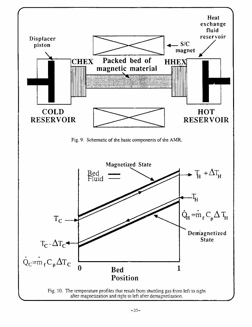
9 Schematic of the basic components of the AMR. 35

10 The temperature profiles that result from shuttling gas from left to 35right after magnetization and right to left after demagnetization.

11 MR using an active magnetic regenerative wheel. 37

12a AMR 20 to 77 K refrigerator performance showing average cooling 40power versus mass flow rate for several values of particle size.

12b AMR 20 to 77 K refrigerator performance showing COP efficiency 40versus mass flow rate for several values of particle size.

12c AMR 20 to 77 K refrigerator performance showing pressure drop 41versus mass flow rate for several values of particle size.

13 Schematic of a multi-stage AMR hydrogen liquefier. 44

iv

LIST OF FIGURES (Cont'd.)

Figure PageNumber Number

14 Effects of the number of stages of the 20 to 77 K AMR hydrogen 45liquefier on performance.

15 Overall efficiency of the 20 to 300 K hydrogen liquefier as a 47function of the efficiency of the 20 to 80 K magnetic liquefier.

16 Effect of AMR period on performance. 48

17 Effect of the field change on performance, expressed in terms of 50the adiabatic temperature change of the ideal magnetic materialat 80 K.

18 Mean wheel diameter versus liquefaction rate of magnetic 52hydrogen liquefier.

19 Complete liquefier system cost as a function of liquefaction rate. 52

V

LIST OF TABLE3

Table PageNumber Nuix-r

I Growth History and Projected Demand for "Small User"Liquid Hydrogen Market 13

II Hydrogen Feedstock Sources and Relative Costs 17

III Relative Prices by Volume frr Merchant Hydrogen 18

IV Operating Costs of an 850 t/d Hydrogen Liquefaction System 19

V Criteria for Selection of Magnetic Materials 27

VI Cost Breakdown of 1 t/d Hydrogen Magnetic Liquefier 51

VII Characteristics of a 533 1/h (1 t/d) Magnetic Hydrogen 53

Liquefier

VIII Cost Breakdown of a 50 kW Supermarket Freezer 56

IX AMR Performance Specifications for 300 K to 80 K Operation 57

X Efficiency Comparison of 1 Ton Per Day All-Gas Hydrogen 60Liquefiers to Magnetic Liquefier Combinations

vi

EVALUATION OF INDUSTRIAL MAGNETIC HEAT PUMP/REFRIGERATORCONCEPTS THAT UTILIZE SUPERCONDUCTING MAGNETS

by

J. A. Waynert, A. J. DeGregoria, R W. Foster, and J. A. Barclay

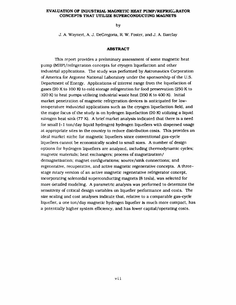
ABSTRACT

This report provides a preliminary assessment of some magnetic heat

pump (MHP)/refrigeration concepts for cryogen liquefaction and other

industrial applications. The study was performed by Astronautics Corporation

of America for Argonne National Laboratory under the sponsorship of the U.S.

Department of Energy. Applications of interest range from the liquefaction of

gases (20 K to 100 K) to cold storage refrigeration for food preservation (250 K to

320 K) to heat pumps utilizing industrial waste heat (350 K to 400 K). Initial

market penetration of magnetic refrigeration devices is anticipated for low-

temperature industrial applications such as the cryogen liquefaction field, and

the major focus of the study is on hydrogen liquefaction (20 K) utilizing a liquid

nitrogen heat sink (77 K). A brief market analysis indicated that there is a need

for small (-1 ton/day liquid hydrogen) hydrogen liquefiers with dispersed usage

at appropriate sites in the country to reduce distribution costs. This provides an

ideal market niche for magnetic liquefiers since conventional gas-cycleliquefiers cannot be economically scaled to small sizes. A number of design

options for hydrogen liquefiers are analyzed, including thermodynamic cycles;

magnetic materials; heat exchangers; process of magnetization/

demagnetization; magnet configurations; source/sink connections; and

regenerative, recuperative, and active magnetic regenerative concepts. A three-

stage rotary version of an active magnetic regenerative refrigerator concept,

incorporating solenoidal superconducting magnets (8 tesla), was selected for

more detailed modeling. A parametric analysis was performed to determine the

sensitivity of critical design variables on liquefier performance and costs. The

size scaling and cost analyses indicate that, relative to a comparable gas-cycleliquefier, a one ton/day magnetic hydrogen liquefier is much more compact, has

a potentially higher system efficiency, and has lower capital/operating costs.

vii

EXECUTIVE SUMMARY

This report presents the results of a study funded by the Argonne National Laboratory (ANL)

for the Office of Industrial Programs (OIP). A subcontract was issued to Astronautics Corporation

of America by ANL. DOE/OIP/ANL's primary interest in magnetic heat pumps (MHPs) is a result

of the potential industrial energy savings that may be achieved through the use of the highly efficient

devices. Further, the discovery of high-temperature superconductors and the desire for alternate

energy conversion devices that do not use chlorofluorocarbons renewed DOE's interest in MHP

technology. MHPs are applicable for all temperature ranges, from liquefaction of gases to cold

storage of foods to industrial heat recovery. With respect to potential energy savings, refrigerator

and heat pump applications near room temperature clearly are where MHPs should be applied.

However, following the workshop held in October 1988 (see page 11) to compare MHPs to vapor

compression devices for near-room-temperature heating and cooling applications, the general

conclusion was that while MHPs could compete on a performance basis, they were presently too

costly to replace existing vapor-compression devices. However, it was suggested that there is a clear

need for more efficient refrigerators in the cryogen liquefaction field, and especially for liquid

hydrogen. Thus, until high-temperature superconductors operating at 77 K or above are

commercially viable, the most appropriate initial industrial market for MHPs is probably in the low-

temperature gas liquefaction sector. In particular, the liquid hydrogen market, with its 20 K

temperature of liquefaction and projected growth rate, appears to offer an ideal market nahe for

magnetic liquefiers. This top-level study assesses whether magnetic liquefiers for hydrogen are

potentially superior to conventional liquefiers on a cost performance basis.

A brief analysis of the liquid hydrogen market indicates that there are presently six large

(typically tens of tons per day, per unit) centralized hydrogen liquefiers in the United States. From

these centralized production centers, liquid hydrogen (LH2) is distributed to perhaps 12 storage

terminals whose locations have been established according to product demand. Here, LH2 is stored

in very large cryogenic tanks. From the terminals, LH2 is trucked to distribution terminals which

also handle other gaseous products. There are perhaps five times as many distribution terminals as

storage terminals. Finally, the product is trucked to the customer. At present, the delivered price of

hydrogen can vary by a factor of ten depending on the quantity used, the distance trucked, and the

form, gaseous or liquid, in which the hydrogen is transported. The transportation distance can have

a major impact on the price to the customer, especially the small user. As an example, the customer

price can be reduced by about 18% if the transportation distance can be decreased from 1500 miles

to under 200 miles. Thus, it appears that the hydrogen market could be expanded through easier

-1-

availability and decreased costs if the distribution system could be economically decentralized

through a dispersed usage of smaller, less costly liquefiers.

Conventional gas cycle liquefiers cannot be economically scaled to the 1 t/d size. A 5 t/d

unit costs about $12.5 million and operates at about 25% efficiency. (Efficiency is used here as the

ratio of the minimum work of liquefaction to the actual work). It is not likely that the efficiency of

conventional units can be maintained as the units are scaled down to the 1 t/d size. It is not

unreasonable to assume the efficiency of a conventional 1 t/d gas cycle liquefier to be 15-20% of

ideal. At best, the capital cost would be $2.5 million. These are the numbers, i.e., an efficiency of

about 20% and capital cost of at least $2.5 million, to which a 1 t/d MHP must be compared.

This study emphasizes an MHP operating between 18 K and 86 K, nominally 20 K to 77 K

with allowance for heat exchange at the cold and hot sinks. It is assumed that liquid nitrogen (LN2 )

is available to precool the hydrogen gas, near atmospheric pressure, to 77 K. The magnetic liquefier

cools and liquefies the precooled hydrogen gas and exhausts heat to the LN2. To achieve reasonable

efficiency of liquefaction, the MHP must incorporate several intermediate temperature stages to

remove the sensible heat and the exothermic energy of the ortho- to para-hydrogen conversion. A

good compromise between efficiency and system complexity is achieved by three stages with

nominal cold temperature operating points of 60 K, 40 K, and 20 K.

A series of design options for both major components and the entire system of the MHP were

analyzed, including thermodynamic cycles; magnetic materials; heat exchangers; process ofmagnetization/demagnetization; magnet configurations; source/sink connections; and regenerative,

recuperative, and active magnetic regenerative concepts. The concept that was selected for more

detailed modeling was a rotary version of an active magnetic regenerative refrigerator (AMR). A

rotary version of the AMR was chosen because it naturally produces continuous cooling, can be

designed with more uniform structural loads, and appears relatively easy to implement. In the rotary

design, a series of parallel-flow, packed-particle beds of magnetic material are assembled into the

form of a ring or wheel. The wheel is actually composed of three I 'P disks with a common axis

of rotation. Each disk is a stage of the AMR. The magnetic field is prOVded by a series of

solenoidal magnets which enclose roughly one-third of the wheel circurerence. There are

manifolds with sliding seals to the beds to allow the appropriate gas flow during heat exchange with

the bed material. In this design, helium gas at 1 MPa (10 atm.) is circulated to communicate

between the hot and cold sinks and the particle bed. The hydrogen gas is cooled by counterflow heat

exchange with the helium gas.

-2-

A parametric performance analysis of the AMR was done considering the effect on the

efficiency of particle size of the bed material, mass flow rate of the helium gas, magnetic field

strength, and frequency of the cycle operation. To perform this analysis, the thermomagnetic

properties of the magnetic material are required. A candidate magnetic material is ErxGd(l-x)Al2 but

to simplify the analysis, ideal magnetic properties were used. Reasonably high efficiency and low

pressure drop across the bed occur for 0.01-cm-diameter particles packed in a bed 5 cm long at 50%

porosity for an 8 T field change with a helium mass flow rate of 0.5 g/s for each square centimeter of

bed cross-section.

Some interesting results were found in a comparison between the magnetic and all-gas cycle

liquefiers. A I t/d /530 !/h) magnetic liquefier is very compact; the mean wheel diameter is 145 cm.

A comparab' Ly cycle liquefier is projected to occupy roughly 5 m x 10 m. The capital cost of the

magnetic liquefier is estimated at $1.07 million versus $2.5 million for the gas cycle device. The

overall efficiency of the hybrid LN2 /magnetic device is 24% versus 20% (projected) for the gas

cycle device. The efficiency diffa'nce represents a 17% reduction in electrical power requirements.

In terms of U.S. energy usage, the rotential amount of energy saved is very small. On the other

hand, the expected hydrogen market expansion should mean many new ventures producing more

jobs. In addition, the use of magnetic refrigeration to liquefy hydrogen is an ideal opportunity to

introduce a new energy-conserving technology which promises to have a much broader range of

future applications, particularly near room temperature.

Based on the results of the analysis described herein, it seems natural to pursue further

development of a magnetic liquefier. We recommend that DOE consider bore research and

development in this area commensurate with their overall objectives.

1. INTRODUCTION

The Office of Indutrial Programs in the U.S. Department of Energy (DOE) and Argonne

National Laboratory (ANL) are active in the development of magnetic heat pumps (MHPs) for

industrial refrigeration applications. Conventional refrigeration technology utilizes gas refrigerants

in a vapor-compression cycle for applications near room temperature and in reverse-Brayton or other

cycles for applications at cryogenic temperature. The conventional technology is well understood,

well established, and mature to the point that there is limited scope for improvement without major

investments.

DOF and ANL recognize that MHPs, with their solid working material, are compact and

offer high efficiency and potentially high reliability at competitive costs. The performance

advantages are especially pronounced in the temperature range below 80 K and especially in

smaller-scale devices. One particular industrial application which appears promising for initial

market penetration is in a relatively small scale (less than 5 ton per day) MHP unit for hydrogen

liquefaction.

This report summarizes the results of an Astronautics Corporation of America (ACA)

contract study for ANL to evaluate magnetic heat pumps with the major application emphasis on the

liquefaction of hydrogen. The objectives of the study are to:

" Establish operating limits and performance characteristics of MHPs for liquefying

hydrogen, considering;* rotating vs. reciprocating devices,

* alternative magnet configurations,

* alternative thermodynamic cycles,

* alternative magnetic materials,

* active magnetic regenerative vs. recuperative/regenerative cycles,

* efficiency, cooling power, and power density, and

* parametric sensitivity studies of magnetic material, cooling capacity, and field

strength;

" Provide a brief assessment of scaling to other low-temperature applications with

differing heat source/sink conditions;

-5-

" Expand and update the previous contract study (Contract No. 81032401) for AYL on

"Impact of High Temperature Superconductors on Room Temperature Magnetic Heat

Pumps/Refrigerators"; and

" Prepare a final report which considers the impact of commercialization of the device

and gives recommendations for future research and development.

The report first presents the principles and history of MHPs in Section 2. Then the present

hydrogen market and the potential market niche for MHPs are discussed in Section 3. Section 4

provides some background on conventional gas-cycle devices for hydrogen liquefaction and then

introduces potential magnetic cycle devices. Section 5 updates previous related MHP studies, while

Section 6 considers other applications up to room temperature. Finally, recommendations for future

work are given in Section 7.

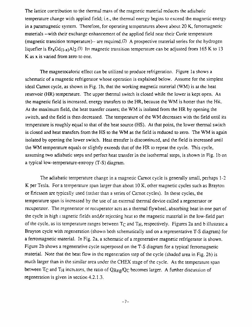
2. BACKGROUND

2.1 Principles of Magnetic Heat Pumps

Heat pumps are similar to refrigerators in that both remove heat from a cold source and

transfer energy to a warm sink under the application of work. Heat pumps and refrigerators differ in

that heat pumps emphasize the heat rejected (as in a space heater) while refrigerators: emphasize the

heat absorbed (as in a freezer). It is common, though, to consider heat pumps as a more general

category which includes refrigerators. That is the approach used throughout this paper, and heat

pump and refrigerator are thus used interchangeably.

Contrary to gas-cycle heat pumps which rely on the expansion and compression of a gas to

achieve the energy transfer from cold to warm sinks, magnetic heat pumps (MHPs) rely on the

magnetocaloric effect. The magnetocaloric effect refers to the reversible change in temperature

exhibited by certain magnetic materials as they experience increasing or decreasing magnetic fields.

Under certain temperature conditions, paramagnetic and ferromagnetic materials warm up upon

adiabatic application of a magnetic field or expel heat at constant temperature if heat transfer is

performed during field application. The process is highly reversible so that adiabatic removal of the

field will cool the material. Conversely, if the temperature is constant during the field reduction,

heat must be absorbed.

The materials commonly used in MHPs are rare earth compounds. For example, gadolinium

gallium garnet(() is a paramagnetic material used in MHPs operating in the 1.8 K to 20 K

temperature range. As the operating temperature is raised, the lattice specific heat increases rapidly.

-6-

The lattice contribution to the thermal mass of the magnetic material reduces the adiabatic

temperature change with applied field; i.e., the thermal energy begins to exceed the magnetic energy

in a paramagnetic system. Therefore, for operating temperatures above about 20 K, ferromagnetic

materials --with their exchange enhancement of the applied field near their Curie temperature

(magnetic transition temperature)-- are required.(2 ) A prospective material series for the hydrogen

liquefier is ErxGd(1-x)Al2.(3) Its magnetic transition temperature can be adjusted from 165 K to 13

K as x is varied from zero to one.

The magnetocaloric effect can be utilized to produce refrigeration. Figure la shows a

schematic of a magnetic refrigerator whose operation is explained below. Assume for the simplest

ideal Carnot cycle, as shown in Fig. 1b, that the working magnetic material (WM) is at the heat

reservoir (HR) temperature. The upper thermal switch is closed while the lower is kept open. As

the magnetic field is increased, energy transfers to the HR, because the WM is hotter than the HR.

At the maximum field, the heat transfer ceases; the WM is isolated from the HR by opening the

switch, and the field is then decreased. The temperature of the WM decreases with the field until its

temperature is roughly equal to that of the heat source (HS). At that point, the lower thermal switch

is closed and heat transfers from the HS to the WM as the field is reduced to zero. The WM is again

isolated by opening the lower switch. Heat transfer is discontinued, and the field is increased until

the WM temperature equals or slightly exceeds that of the HR to repeat the cycle. This cycle,

assuming two adiabatic steps and perfect heat transfer in the isothermal steps, is shown in Fig. 1 b on

a typical low-temperature-entropy (T-S) diagram.

The adiabatic temperature change in a magnetic Carnot cycle is generally small, perhaps 1-2

K per Tesla. For a temperature span larger than about 10 K, other magnetic cycles such as Brayton

or Ericsson are typically used (rather than a series of Carnot cycles). In these cycles, the

temperature span is increased by the use of an external thermal device called a regenerator or

recuperator. The regenerator or recuperator acts as a thermal flywheel, absorbing heat in one part of

the cycle in high r.iagnetic fields and/r rejecting heat to the magnetic material in the low-field part

of the cycle, as its temperature ranges between TC and TH, respectively. Figures 2a and b illustrate a

Brayton cycle with regeneration (shown both schematically and on a representative T-S diagram) for

a ferromagnetic material. In Fig. 2a, a schematic of a regenerative magnetic refrigerator is shown.

Figure 2b shows a regenerative cycle superposed on the T-S diagram for a typical ferromagnetic

material. Note that the heat flow in the regeneration step of the cycle (shaded area in Fig. 2b) is

much larger than in the similar area under the CHEX stage of the cycle. As the temperature span

between TC and TH incrt ases, the ratio of QReg/QC becomes larger. A further discussion of

regeneration is given in section 4.2.1.3.

-7-

LIHR

THERMAL SWITCH

WM MAGNET

HS

Fig. Ia. A simple magnetic refrigerator.

-

Entropy (S/R)

Field Strength (T)

o 0.0

f 0.5

0 1.5

* 2.0

o] 2S

A 3.0

e 3.5

* 4.0

.. 4.5

* 5.0

x 6.0

X 7.0

* 8.0

. 9.0

Fig. 1 b. Temperature--entropy cycle followed by the magneticmaterial undergoing a Carnot cycle.

V-8-

0

0

S..0JH

J

High FieldRegion

HEAT REJECTION

RegenerationHIGH TEMPERATURE (Hot=Cold)HEAT EXCHANGER

ADIABATIC

MAGNETIZATION

ADIABATIC

DEMAGNETIZATION

litE -LOW TEMPERATURE

Regeneration HEAT EXCHANGE(Cold =Hot)

WORK

4- Zero field region

HEAT ABSORPTION

Fig. 2a. Schematic of a regenerative magnetic refrigeratorfor near room temperature operation.

T i

T

Tc

AdiabaticDemagnetization

HHEX Ba>>O

Adiabatic.\Magnetization

------------------------------- ---------------- B a~=0

Regeneration

--------- -------- \c

Q Re;

C H EX

QC

Fig. 2b. Temperature--entropy cycle with regeneration showing the heat flowswhich must be accomplished during each cycle.

-9-

The terms regeneration and recuperation are not uniquely defined in the refrigeration

community. In this report, regenerative heat exchange refers to thermal energy exchange in which

the temperature distribution is time-dependent, i.e., periodic. An example is a packed-particle bed of

lead shot in which warm gas flows in one direction, depositing heat into the bed, followed by heat

recovery as cold gas flows through the bed in the opposite direction. Thus, the temperature

distribution in the bed varies with time. In contrast, a recuperative heat exchanger has a temperature

distribution which is time-independent. A temperature gradient exists in the device, but the

temperature at each point does not vary in time. A common example is the counter-flow heat

exchanger.

Magnetic refrigeration offers a third and unique possibility for the thermal flywheel of which

there is no counterpart in gas-cycle devices. It is possible to use the working magnetic material as

the regenerator. This regenerator is referred to as an active magnetic regenerator or AMR and

refrigerators based on this regenerator are also referred to as AMRs. The AMR is the focal point of

this study. The MHP hydrogen liquefaction concept considered in this study operates between about

18 K and 86 K and thus, requires regeneration. Because the heat absorbed/rejected by the

regenerator is several times larger than the heat absorbed from the source in a single cycle, it is

evident that excellent heat transfer during regeneration is required to obtain high efficiency. Also,

higher fields yield greater cooling power with minimal increase in losses. This means higher

efficiencies result from higher magnetic fields; thus, the need for superconducting magnets.

In addition to factors concerning the magnetic material, superconducting magnets, and

excellent heat transfer to and from the magnetic material, there are other important considerations in

the design of MHPs. Forces within the magnets, between magnets, and between the magnets and

magnetic material can be large. Thus, an effective supporting structure is required to react to these

forces. Some type of drive mechanism is needed to change the relative position of the magnetic

material and the magnets to achieve the magnetization and demagnetization. Dewars and external

heat exchangers are also required. Various sensors are needed to provide power, monitor

temperatures and flow rates, and control the MHP.

2.2 History of Magnetic Heat Pumps

The discovery of the magnetocaloric effect (MCE) occurred in 1918 when A. Piccard and P.

Weiss(4) experimentally separated irreversible hysteretic heating from reversible heating and cooling

upon magnetic field cycling. The metallic ferromagnet Ni was used in their experiments near its

Curie temperature of 3580C (631 K). In 1934 the effect was demonstrated in Fe metal(5 ) at over

-10-

1000 K. Closer to room temperature, the effect in Gd metal (292 K) has only relatively recently

been measured.(6 )

An early examination of the use of the MCE of ferromagnets in heat pumps was presented in

1948 when Iskendrian and Brillouin( 7 ) described the magnetic thermodynamics of a useful cycle.

Following this analysis, thermomagnetic heat engines using ferromagnetic working materials in the

form of direct thermal to electrical energy converters were proposed.(8 ) The efficiencies of the

Carnot cycle convertors were low and the devices were not cost-competitive with other heat engines.

More recently, regenerative-cycle (Ericsson) thermomagnetic generators have been proposed which

offer much higher efficiencies.( 9 ,10) No major development programs presently exist on these

promising devices.

After the discovery of ferrofluids, i.e., stable colloidal suspensions of ferromagnetic particles

in carrier fluids, in 1965(11), there was a burst of activity on the use of ferrofluids as working

materials in heat engines.( 12-13) Although it is not clear from most of the published analyses of the

thermodynamic cycles in the use of ferrofluids in MHPs, the MCE is the basis of operation in these

units. Devices were actually demonstrated but the concentration of ferromagnetic particles (Fe2O3)

in ferrofluids could not be increased enough to make them viable. Operation well below the Curie

temperature and the thermal addenda from the carrier fluid made the effective adiabatic temperature

change of the Fe2O3 particles about 0.1 K. Concentrated suspensions of gadolinium particles in

mercury were investigated for near-room-temperature devices but the suspensions were not stable in

applied fields.( 14 )

The first proposed use of the MCE of solid ferromagnets in magnetic heat pumps near room

temperature was made by Brown( 15 ) in the early 1970's when the ".energy crisis" made high

efficiency in thermal devices a strong technology driver. A reciprocating design using Gd metal, a

7 T magnetic field, and an alcohol-water mixture as the liquid regenerator was successfully operated

in 1976.(16) This device ultimately spanned about 800C around the Curie point of Gd (292 K) with

no external thermal load. This pioneering work formed the basis of research and development

programs at several laboratories around the world.

In parallel with the characterization and eventual use of magnetocaloric effect in

ferromagnets above about 20 K, the use of the MCE in paramagnets at temperatures below 20 K was

pursued. From 1926(17-18) until 1966(19), the technique was used exclusively for very small cooling

powers (microwatts) below 1 K. From 1966 to present, significant effort has been put into

-11-

developing larger-cooling-power (watts) Carnot-cycle devices operating in the 1 K to 20 K

region.(20)

Most of the work on magnetic refrigerators has been for cryogenic applications( 2O.21, 2 2) but

several laboratories such as Idaho National Engineering Laboratory and David Taylor Research and

Development Center have worked on room-temperatures devices. Several proof-of-concept devices

for near-room-temperature operation have been built.(23-26 ) None of these devices has demonstrated

efficiencies and reliabilities that match original predictions but the results were encouraging enough

to move toward engineering prototypes.

In the last three years, the discovery of high-temperature superconductors and the recognition

of the seriousness of ozone depletion by chlorofluorocarbons have increased interest in magnetic

heat pump technology.( 27 ) The DOE Office of Industrial Programs sponsored a workshop in the fall

of 1988 at Herndon, VA, to assess whether magnetic heat pumps at room temperature could

effectively compete with vapor-compression-cycle devices (VCD).( 28) As a result of this meeting it

was concluded that although magnetic heat pumps may compete with VCDs on a performance basis,

they could not presently compete on a cost basis. Alternatively, MHP's were suggested as

potentially economically viable for lower-temperature applications such as hydrogen liquefiers. A

better definition of the potential of MHPs as liquefiers in comparison to conventional gas-cycle

devices is an objective of this report.

3. LIQUID HYDROGEN MARKET AND POTENTIAL IMPACTOF A MAGNETIC LIQUEFIER

3.1 Overview of the Hydrogen Market

The energy content of the presently consumed commercial hydrogen accounts for 0.9% of

the total U.S. energy consumption. While commercial hydrogen usage is small in terms of national

energy consumption, hydrogen is a critical feed stock in ammonia production, methanol production,

and petroleum refining. These commercial uses form the "Large User Hydrogen" marketplace.

Within the Large User Hydrogen marketplace, there is a segment comprising the "Small User" of

hydrogen. This marketplace includes such uses as the synthesis of chemicals, metallurgical

processing, electronic component manufacture, vegetable oil processing, and others. The small user

hydrogen market is a growing market and is presently paying the highest prices for hydrogen. The

history and projected demand for small user hydrogen through the year 2000 is illustrated in Table

I.(29) Wiuiiin the small user hydrogen market, the growth history and future growth projections of

the merchant hydrogen subsector share the same characteristics, i.e., a history of high growth rate

and a projected future of high growth rate .(29)

-12-

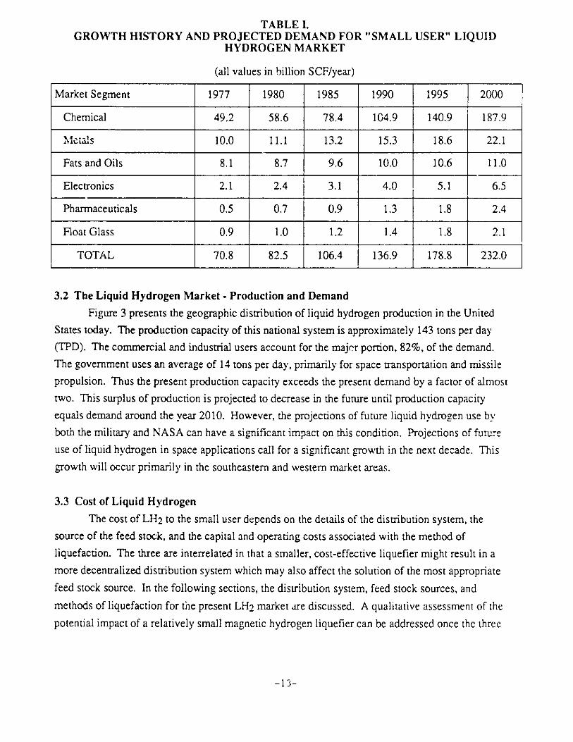
TABLE I.GROWTH HISTORY AND PROJECTED DEMAND FOR "SMALL USER" LIQUID

HYDROGEN MARKET

(all values in billion SCF/year)

Market Segment 1977 1980 1985 1990 1995 2000

Chemical 49.2 58.6 78.4 104.9 140.9 187.9

Metals 10.0 11.1 13.2 15.3 18.6 22.1

Fats and Oils 8.1 8.7 9.6 10.0 10.6 11.0

Electronics 2.1 2.4 3.1 4.0 5.1 6.5

Pharmaceuticals 0.5 0.7 0.9 1.3 1.8 2.4

Float Glass 0.9 1.0 1.2 1.4 1.8 2.1

TOTAL 70.8 82.5 106.4 136.9 178.8 232.0

3.2 The Liquid Hydrogen Market- Production and Demand

Figure 3 presents the geographic distribution of liquid hydrogen production in the United

States today. The production capacity of this national system is approximately 143 tons per day

(TPD). The commercial and industrial users account for the major portion, 82%, of the demand.

The government uses an average of 14 tons per day, primarily for space transportation and missile

propulsion. Thus the present production capacity exceeds the present demand by a factor of almost

two. This surplus of production is projected to decrease in the future until production capacity

equals demand around the year 2010. However, the projections of future liquid hydrogen use by

both the military and NASA can have a significant impact on this condition. Projections of future

use of liquid hydrogen in space applications call for a significant growth in the next decade. This

growth will occur primarily in the southeastern and western market areas.

3.3 Cost of Liquid Hydrogen

The cost of LH2 to the small user depends on the details of the distribution system, the

source of the feed stock, and the capital and operating costs associated with the method of

liquefaction. The three are interrelated in that a smaller, cost-effective liquefier might result in a

more decentralized distribution system which may also affect the solution of the most appropriate

feed stock source. In the following sections, the distribution system, feed stock sources, and

methods of liquefaction for the present LH2 market are discussed. A qualitative assessment of the

potential impact of a relatively small magnetic hydrogen liquefier can be addressed once the three

-13-

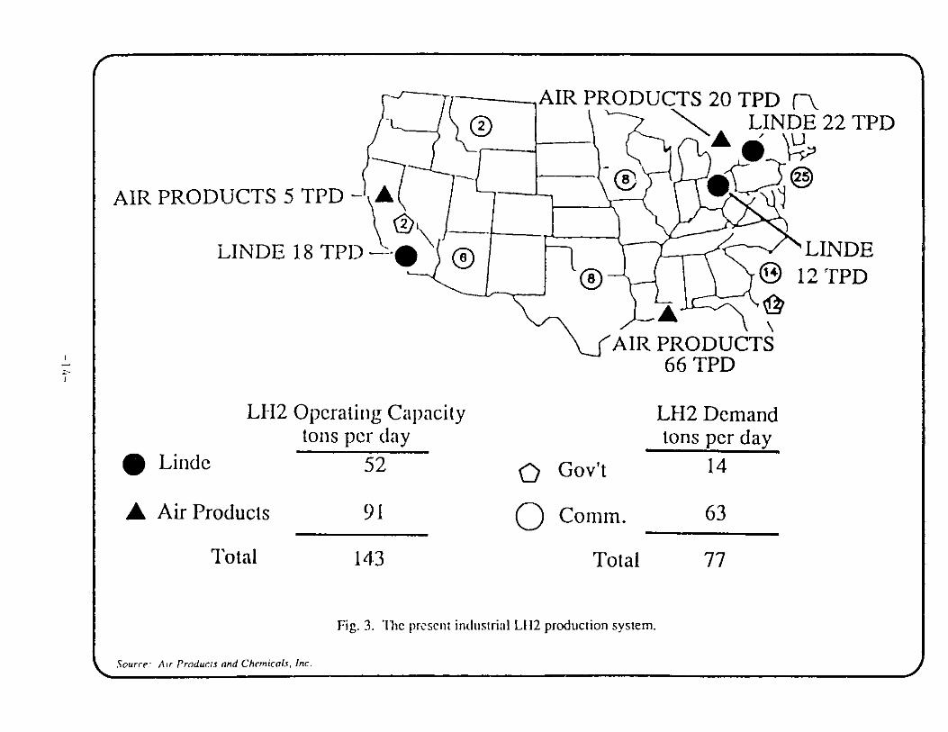
AIR PRODUCTS 20 TPD (\LINDE 22 TPD

AIR PRODUCTS 5 TPD A

LINDE 18 TPD -- _LINDE

1 2 TPD

AIR PRODUCTS66 TPD

LH2 Operating Capacity LH2 Demandtons per (lay tons per day

Linde 52 0 Gov't 14

A Air Products 91 0 Comm. 63

Total 143 Total 77

Fig. 3. 1e present industrial LH2 production system.

YSourre: Air Products and Chemicals. Inc. low,

4%

%.ft 000IN

cost factors (distribution, feed stock, liquefier) are understood. A quantitative assessment of the

impact is beyond the scope of this report.

3.3.1 Distribution

The present liquid hydrogen (LH2) distribution system is based o the centralized location of

production facilities. A liquid hydrogen product is shipped by truck from the large centralized

production facilities to liquid hydrogen terminals, perhaps ten in number, which make up a second

level of the distribution system. At these liquid hydrogen terminals, the bulk product is stored in

large cryogenic tank systems. The liquid hydrogen product is then reshipped to supply a system of

20 to 30 distribution terminals which also sell other gas products. From the distribution terminals,

the liquid hydrogen product is again moved by cryogenic tanker trucks to the customer locations.

The local delivery costs significantly contribute to the delivery price of the hydrogen product. For

example, there is an 18% reduction in the liquid hydrogen sales price if the hauling distance can be

reduced from 1500 to 200 miles.( 3 0) Clearly, the cost of shipment from the centralized production

facility to the hydrogen terminals to the distribution points and finally to the customer represent a

significant portion of the final deiX'ered product price.

Customer annual demand determines the form of delivery of the hydrogen product. Low

demands can be serviced with compressed gas cylinders. However, this delivery is the most

expensive in terms of cost per unit volume or per unit weight delivered. As the customer demand

increases, liquid hydrogen product becomes the most economical delivered form. Recent

improvements in cryogenic storage technology have resulted in a trend towards moving liquid

product delivery into market segments that have been historically serviced by compressed gas

cylinder sales. There is an effort to convert compressed gas cylinder buyers who require annual

volumes as low as one million standard cubic feet (SCF) per annum to the use of liquid hydrogen.

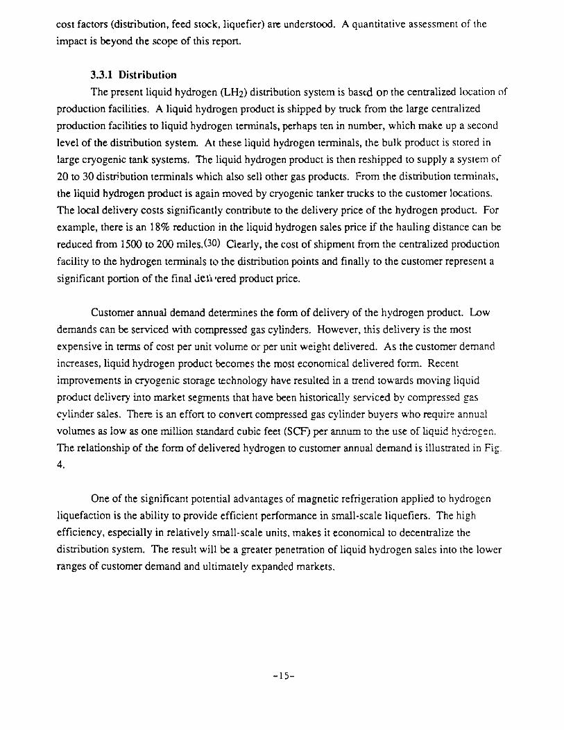
The relationship of the form of delivered hydrogen to customer annual demand is illustrated in Fig.

4.

One of the significant potential advantages of magnetic refrigeration applied to hydrogen

liquefaction is the ability to provide efficient performance in small-scale liquefiers. The high

efficiency, especially in relatively small-scale units, makes it economical to decentralize the

distribution system. The result will be a greater penetration of liquid hydrogen sales into the lower

ranges of customer demand and ultimately expanded markets.

-15-

11111 10

Present Industry Sales Program - practical LH2sales for 1 mmscf/annum customers

Magnetic Liquefaction

Range of liquid sales

Range of bulk sales

Range of cylinder sales

Hlydrogren Demandmillion SCF per year

Fig. 4. The relationship of the form of delivered ydrogen to customer annual demand.

Reference: JPL final report to DOEIN1IASr contract No. 955492, June 195r.. J

10-2 10I

fl**O- - -

_A%,*,4

00p,

10

I I I I I

10~ I

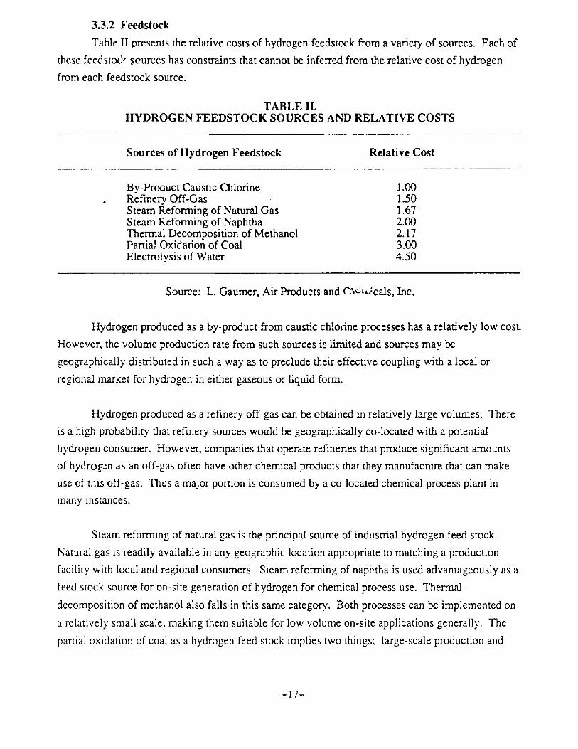
3.3.2 Feedstock

Table II presents the relative costs of hydrogen feedstock from a variety of sources. Each of

these feedstoc c sources has constraints that cannot be inferred from the relative cost of hydrogen

from each feedstock source.

TABLE H.HYDROGEN FEEDSTOCK SOURCES AND RELATIVE COSTS

Sources of Hydrogen Feedstock Relative Cost

By-Product Caustic Chlorine 1.00Refinery Off-Gas 1.50Steam Reforming of Natural Gas 1.67Steam Reforming of Naphtha 2.00Thermal Decomposition of Methanol 2.17Partial Oxidation of Coal 3.00Electrolysis of Water 4.50

Source: L. Gaumer, Air Products and (C'-ecals, Inc.

Hydrogen produced as a by-product from caustic chlorine processes has a relatively low cost.

However, the volume production rate from such sources is limited and sources may be

geographically distributed in such a way as to preclude their effective coupling with a local or

regional market for hydrogen in either gaseous or liquid form.

Hydrogen produced as a refinery off-gas can be obtained in relatively large volumes. There

is a high probability that refinery sources would be geographically co-located with a potential

hydrogen consumer. However, companies that operate refineries that produce significant amounts

of hydrown as an off-gas often have other chemical products that they manufacture that can make

use of this off-gas. Thus a major portion is consumed by a co-located chemical process plant in

many instances.

Steam reforming of natural gas is the principal source of industrial hydrogen feed stock.

Natural gas is readily available in any geographic location appropriate to matching a production

facility with local and regional consumers. Steam reforming of napibtha is used advantageously as a

feed stock source for on-site generation of hydrogen for chemical process use. Thermal

decomposition of methanol also falls in this same category. Both processes can be implemented on

a relatively small scale, making them suitable for low volume on-site applications generally. The

partial oxidation of coal as a hydrogen feed stock implies two things: large-scale production and

-17-

significant environmental impacts. For this reason this process is not used to any great extent in the

production of industrial hydrogens feed stock.

The electrolysis of water offers hydrogen feed stock availability in small scales using

equipment that is relatively simple to operate. However, as can be seen from Table II, electrolysis-

generated hydrogen feedstock is the most expensive source. When viewed in light of the premium

prices paid for delivered hydrogen by small users, as presented in Tabk III, electrolysis-generated

hydrogen feedstock for liquefaction may find some niches in the meienant hydrogen marketplace.

The general promise of magnetic liquefiers, i.e., high efficiency in small-scale systems, is

appropriate to considering this type of application.

TABLE III.RELATIVE PRICES BY VOLUME FOR MERCHANT HYDROGEN

Individual Customer Demand(Million SCF/yr)

0.200.350.500.503.05.0

10.012.01 R.6

22.07.0

72.097.0

100.0120.0150.0180.0200.0

Relative Delivered Price of Hydrogen$/KSCF

7.593.937.573.031.101.661.311.261.190.961.101.100.830.790.971.060.831.0

3.3.3 Liquefaction

The cost of liquefaction must be considered from two perspectives:

" the capital investment required to construct and bring the liquefaction plant to an

operational status; and

* the cost of operation of that liquefaction plant.

-18-

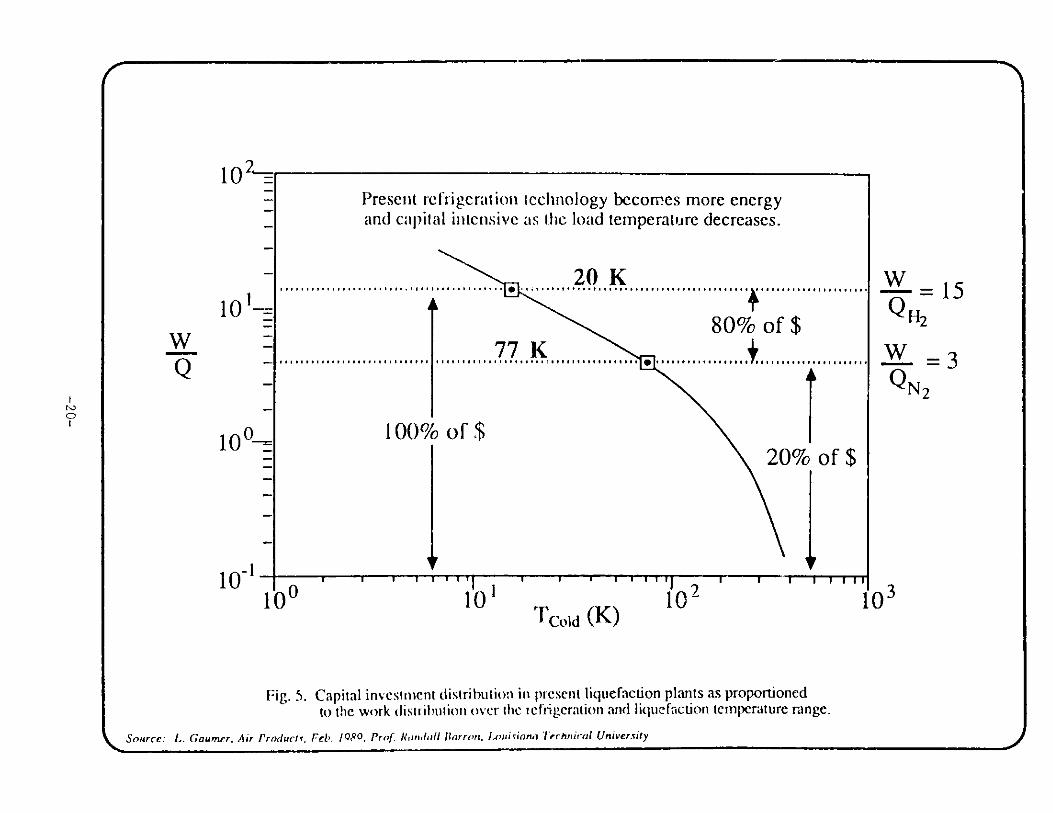
In terms of both these costs accounts, if more efficient, compact, and lower-cost magnetic liquefiers

are developed, they will offer significant advantages to users of liquid hydrogen.

Figure 5 illustrates two things. First, it takes about five times more work to produce a unit of

cooling power at 20 K LH2 temperature than it does at 77 K LN2 temperature. Second, 20% of the

capital cost of a hydrogen liquefier goes into cooling the hydrogen to 77 K, while 80% of the capital

cost goes into achieving the 20 K stage.

Compact, low-cost magnetic refrigeration applied to the 80 K to 20 K stage offers the

opportunity for achieving significantly lower capital investments than those presently made in

mechanical refrigeration systems operating over the same temperature range. This is the principal

mechanism of impact of magnetic refrigeration on capital investments costs.

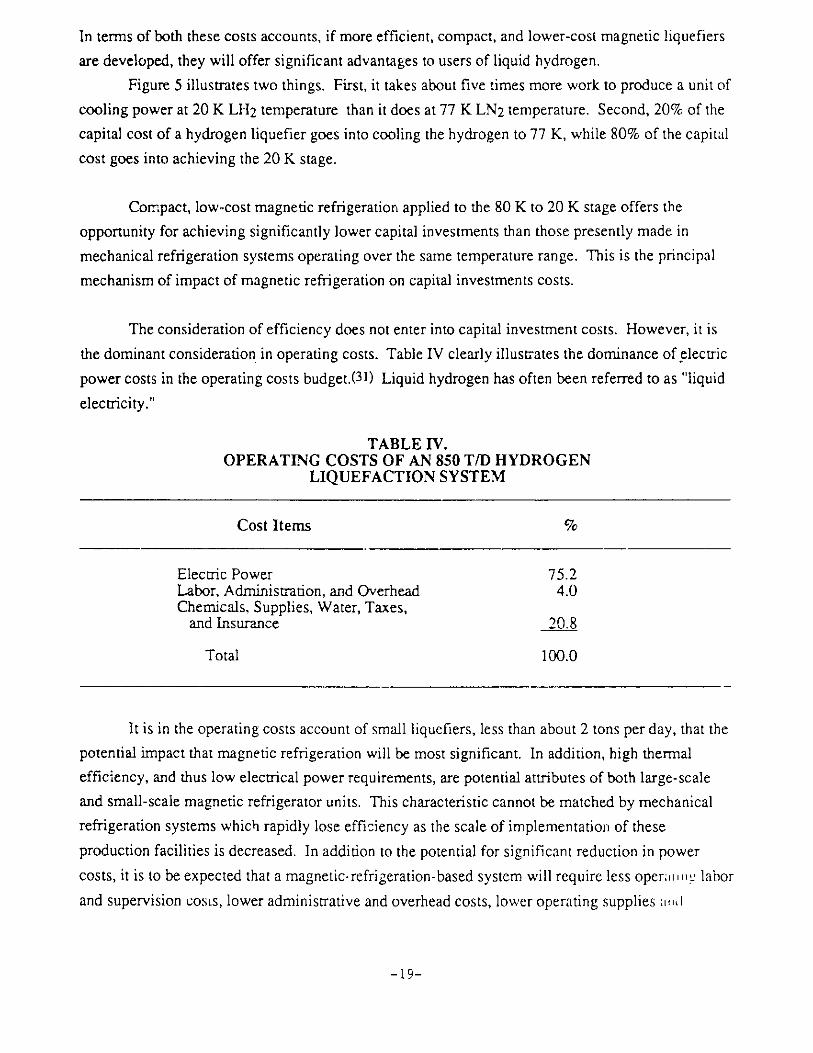
The consideration of efficiency does not enter into capital investment costs. However, it is

the dominant consideration in operating costs. Table IV clearly illustrates the dominance of electric

power costs in the operating costs budget.(3 1 ) Liquid hydrogen has often been referred to as "liquid

electricity."

TABLE IV.OPERATING COSTS OF AN 850 T/D HYDROGEN

LIQUEFACTION SYSTEM

Cost ItemsF%

Electric Power 75.2Labor, Administration, and Overhead 4.0Chemicals, Supplies, Water, Taxes,

and Insurance 20.8

Total 100.0

It is in the operating costs account of small liquefiers, less than about 2 tons per day, that the

potential impact that magnetic refrigeration will be most significant. In addition, high thermal

efficiency, and thus low electrical power requirements, are potential attributes of both large-scale

and small-scale magnetic refrigerator units. This characteristic cannot be matched by mechanical

refrigeration systems which rapidly lose efficiency as the scale of implementation of these

production facilities is decreased. In addition to the potential for significant reduction in power

costs, it is to be expected that a magnetic-refrigeration-based system will require less operaiun labor

and supervision costs, lower administrative and overhead costs, lower operating supplies ;nd

-19-

Present refrigeration technology becomes more energyand capital intensive as the load temperature decreases.

80% of $se.... .. 0 0.... .. .. .. . $.. . . ................ ,. ..... .......... ........ ..... ........

100%o of $

20% of $

-I .-. -. -

10i

w- = 15

w H2

- = 3N 2

1 I I I 3O

Tcola (K)

Fig. S. Capital investment distribution in present liquefactioto the work (Iiditr ibtion over the rcfrigcration and lik

IL~ Source: L. Gaurne'r. Air Producs. Feb'. I980, Pro-f. Rajndall flarrwzn. I,ouirciana Ierhniraul University

rn plants as proportionedtiefaction temperature range.

I

10

110WQ

10 =

II10-

rO*M*N

A- -

Soo

I I

100

opr

maintenance costs, and finally lower taxes and insurance costs (which are usually computed on a

percent of investment cost basis).

Thus it is probable that magnetic-refrigeration-based hydrogen liquefaction systems will be

characterized by significantly lower capital investment cost and operating costs. Further, this

potential advantage will be available in both large-scale and small-scale installations.

4. LIQUEFACTION OF HYDROGEN

4.1 Gas-Cycle Liquefiers

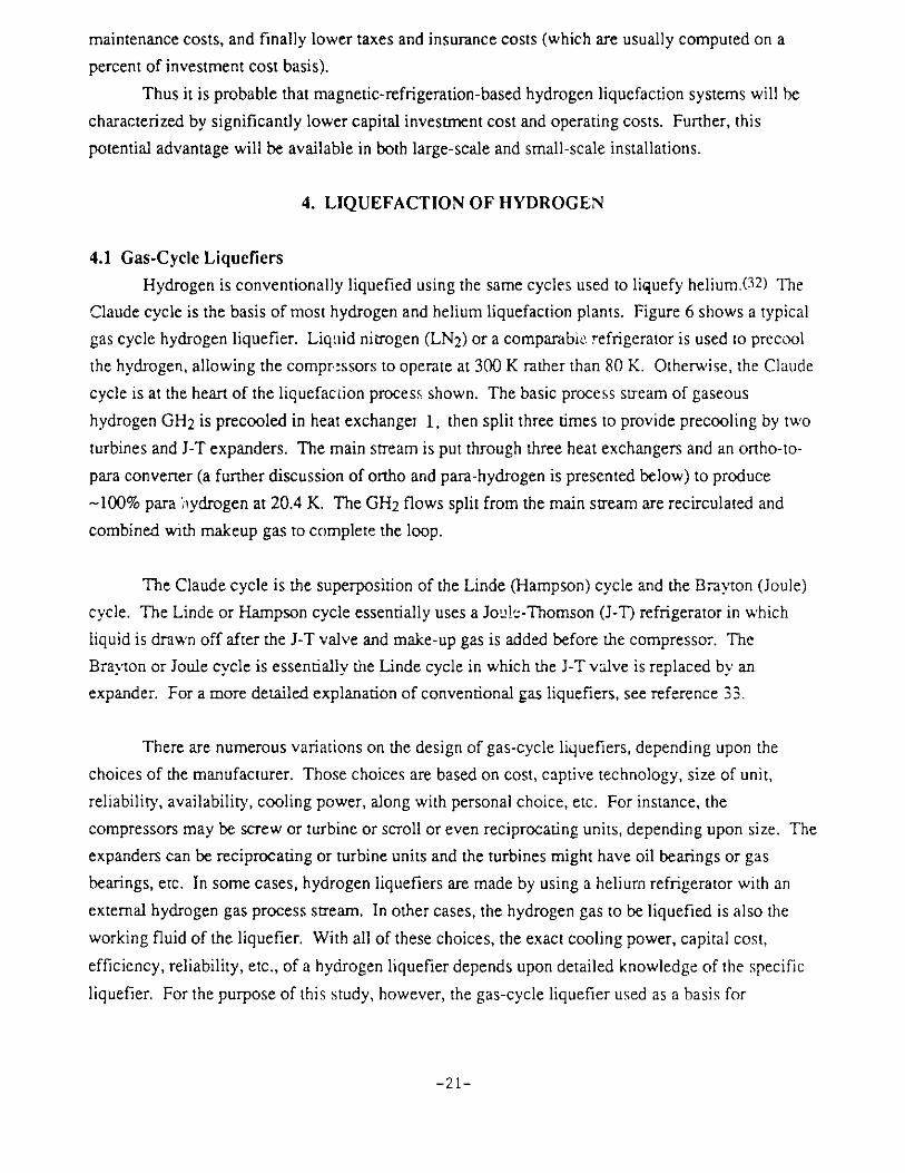
Hydrogen is conventionally liquefied using the same cycles used to liquefy helium.( 32 ) The

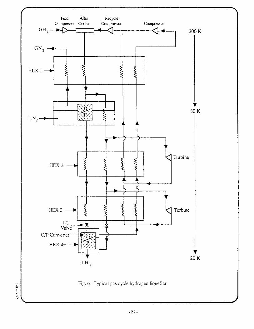
Claude cycle is the basis of most hydrogen and helium liquefaction plants. Figure 6 shows a typical

gas cycle hydrogen liquefier. Liquid nitrogen (LN2) or a comparab e refrigerator is used to precool

the hydrogen, allowing the compressors to operate at 300 K rather than 80 K. Otherwise, the Claude

cycle is at the heart of the liquefaction process shown. The basic process stream of gaseous

hydrogen GH2 is precooled in heat exchanger 1, then split three times to provide precooling by two

turbines and J-T expanders. The main stream is put through three heat exchangers and an ortho-to-

para converter (a further discussion of ortho and para-hydrogen is presented below) to produce

~100% para >ydrogen at 20.4 K. The GH2 flows split from the main stream are recirculated and

combined with makeup gas to complete the loop.

The Claude cycle is the superposition of the Linde (Hampson) cycle and the Brayton (Joule)

cycle. The Linde or Hampson cycle essentially uses a Joul:-Thomson (J-T) refrigerator in which

liquid is drawn off after the J-T valve and make-up gas is added before the compressor. The

Bravton or Joule cycle is essentially the Linde cycle in which the J-T valve is replaced by an

expander. For a more detailed explanation of conventional gas liquefiers, see reference 33.

There are numerous variations on the design of gas-cycle liquefiers, depending upon the

choices of the manufacturer. Those choices are based on cost, captive technology, size of unit,

reliability, availability, cooling power, along with personal choice, etc. For instance, the

compressors may be screw or turbine or scroll or even reciprocating units, depending upon size. The

expanders can be reciprocating or turbine units and the turbines might have oil bearings or gas

bearings, etc. In some cases, hydrogen liquefiers are made by using a helium refrigerator with an

external hydrogen gas process stream. In other cases, the hydrogen gas to be liquefied is also the

working fluid of the liquefier. With all of these choices, the exact cooling power, capital cost,

efficiency, reliability, etc., of a hydrogen liquefier depends upon detailed knowledge of the specific

liquefier. For the purpose of this study, however, the gas-cycle liquefier used as a basis for

-21-

Feed After RecycleCompressor Cooler Compressor

G H2 W-ll -

_____U'I

____4

4

HEX 2

I

Compesso

Compressor

300 K

80 K

Turbine

fri

HEX 3 -Turbine

J TValve

O/P Converter--

HEX 4--

20 KLH

Fig. 6. Typical gas cycle hydrogen liquefier.

-22-

GN 2

HEX i -*

LN,-

4-

\ 4. M.Wooo

A6-

i

comparison to a magnetic liquefier is only an average unit, i.e., a generic Claude-cycle unit which is

close to state of the art. The efficiency of gas-cycle liquefiers varies slightly with designs above 5

tons per day (t/d) to 30 t/d, the relative Carnot efficiency of the liquefier is 20-25%. The capital

costs and operating costs of hydrogen liquefiers is such that gas-cycle plants smaller than about 5 t/d

are not economically feasible.( 27 )

The liquefaction of hydrogen imposes a unique additional complication in that the hydrogen

molecule exists in different forms. A high-energy ortho (0) state and a low-energy para (P) state

exist depending on whether the nuclear spins of the protons are aligned or anti-aligned, respectively.

Above about 20 K there is a significant quantity of ortho-hydrogen in an equilibrium state, the

amount increasing with temperature from about 0.2% at 20 K to 50% at 77 K to about 75% at

300 K. Because of the relatively slow natural conversion rate and because of the large amount of

energy given off during the conversion, catalytic converters are used at various temperatures in

liquefaction plants. One converter at 77 K provides good efficiency for 0 to P conversion from 300

K to 77 K. Several more converters are required to achieve high efficiency between 77 K and 20 K.

4.2 Magnetic-Cycle Liquefiers

Given that typical gas-cycle liquefiers presently are not cost-effective below about 5 t/d and

given that there appears to be a market for a 1-2 t/d hydrogen liquefier, the obvious question is to

address whether a magnetic liquefier is cost effective at the 1-2 t/d size.

With this in mind, a magnetic-cycle liquefier composed of a liquid nitrogen heat sink and

precooler plus a 77 K to 20 K magnetic refrigerator is the simplest unit to compare to a conventional

gas-cycle liquefier. The boiled-off nitrogen gas (GN2) at 77 K can be used to precool the incoming

hydrogen process stream from 300 K to near 77 K in a counterflow heat exchanger. There is ample

sensible heat available from the nitrogen gas evolved by the magnetic stage to precool the hydrogen

stream. The excess sensible heat in GN2 could be used to cool thermal shields which intercept

radiant energy normally incident on lower temperature structures. The 0-to-P conversion to obtain

equilibrium hydrogen at 77 K before entering the 77 K to 20 K magnetic stage can occur in a single

converter in the LN2 tank. (It can be shown that there is negligible benefit in doing the 0-to-Pconversion in more than one stage above 77 K.)

Our computations indicate that a 1 t/d hydrogen liquefier would boil off about 27 t/d of LN2 .

The location of the LN2 supply is a factor in the ultimate cost of LH2 produced by the magnetic

liquefier. Whether it is more economical to truck in this quantity of LN2, or to produce it on site is

beyond the scope of this report. For cost comparisons we have taken delivered LN2 prices.

-23-

4.2.1 Magnetic Refrigerator Design Options

The design of a magnetic refrigerator (MR) involves selecting design parameters for each

major component of the system. The rational for various selections is presented in subsequent

subsections.

The design of an MR begins with the primary specifications of the intended application: for

example, the load to be cooled, the temperature at which the load is to be cooled, and the sink

temperature and method of rejecting heat from the MR. The objectives for this study specified a

heat rejection temperature of 77 K provided by vaporization of LN2. Thus, the MR must cool H2

from 77 K to 20.27 K and liquefy it at a rate of 1 t/d with heat rejection to boiling LN2. The first

choice to be made in the design of a MR for this application involves the refrigeration cycle.

4.2.1.1 Refrigeration Cycle

A suitable thermodynamic refrigeration cycle must be performed to use the magnetocaloric

effect in a refrigerator. The MR may be designed to operate with one of several possible cycles as

summarized in Fig. 7; each cycle has advantages and disadvantages for particular operation

conditions. Some of the differences in the suitability of various cycles at different operating

temperatures can be illustrated by considering the "adiabatic temperature change." The adiabatic

temperature change upon magnetization or demagnetization is given by

ATs = -T ( a dBCB DT B

where C3 is the heat capacity at constant flux density, M is the magnetizadon, and B is the external

flux density. Because the adiabatic temperature change is inversely proportional to CB, which

increases sharply above about 20 K, appreciable ATs can only be obtained by a large SM/ST above

-20 K. Therefore, the materials required for thermodynamic cycles are paramagnets below -20 K

and ferromagnets above ~20 K. The thermodynamic cycles differ somewhat above and below -20

K because of the change in CB. The magnetic cycles shown in Fig. 7 are analogous to gas cycles. A

general description of these cycles is given below.

4.2.1.1.1 Carnot Cycle. The Carnot cycle consists of two isothermal

processes and two isentropic processes that are easy to perform in a magnetic system. Consider a

ferromagnetic material near its Curie temperature: the material can be isolated from, or put in

contact with, hot and cold baths at will. The first step is an iosthermal magnetization while the

-2J -

material is in contact with the hot bath; the heat of magnetization is rejected into the hot bath. Next,

an isolated (isentropic) partial demagnetization cools the material. The third step puts the material

in contact with the cold bath while demagnetization continues to zero field, and heat is absorbed

from the cold bath. The final step is an isentropic partial magnetization back to the original starting

temperature. These two isothermal processes and two isentropic processes constitute a magnetic

Carnot cycle as shown in Fig. 7. The temperature span of a Carnot cycle above about 20 K is

limited to 5-10 K with about 10 T field change, but no regeneration is required. Larger temperature

spans require other cycles.

4.2.1.1.2 Brayton Cycle. The Brayton cycle consists of two isentropic

processes and two isofield processes. With regeneration it can cover much larger temperature spans

than a Carnot cycle. The Brayton cycle is very attractive because it can be coupled easily to the

external heat exchanger through the temperature change caused by the isentropic field changes, as

illustrated in Fig. 7.

4.2.1.1.3 Ericsson and Stirling Cycles. An Ericsson cycle consists of two

isothermal processes, and two isofield processes (Fig. 7). The Stirling cycle requires two isothermal

processes and two isomagnetization processes as shown in Fig. 7. Both cycles require regeneration

to span large temperature differences. These cycles require excellent heat transfer between the heat-

exchange fluid and the source and sink to attain the isothermal process. Thus, the Brayton cycle is

easier to implement in a practical device.

4.2.1.2 Magnetic Materials

To execute any thermodynamic refrigeration cycle, an entropy change must occur. For

magnetic cycles, the entropy change is caused by the application or removal of a magnetic field to a

paramagnetic or ferromagnetic material. Generally, paramagnets are used below, and ferromagnets

are used above ~20 K.

The criteria for selection of ferromagnets and paramagnets are similar with regard to thermal,

chemical, physical, and mechanical properties. A summary of these criteria is presented in Table V.

Based on the above criteria, gadolinium compounds are among the best initial choices as

magnetic refrigerants. Gadolinium may be made into a wide variety of ferromagnetic compounds

with transition temperatures ranging from below 20 K to near 300 K. For the present study, the

thermomagnetic properties of ErxGd(..x)Al2 have been calculated using mean-field theory for the

magnetic properties and the Debye model for the thermal properties. The value of x was chosen to

provide an ordering temperature of 85 K, as required. The calculated properties are estimated to be

-25-

Brayton

isentropic (adiabatic)

B>>0 stages

Ericsson

B=0

B 0 isothermal

Stirling

B=O

B >O

T

constant

magnetizationstages

T

Fig. 7. Magnetic entropy-temperature diagrams illustrating several thermodynamic cycles with ferromagnetic materials.

J

Carnot

6 = 0

B>>0

S

S

r

rv

accurate to 10-20%. Blending of these or similar compounds can be done to provide close to ideal

materials for actual cycles.

TABLE V.CRITERIA FOR SELECTION OF MAGNETIC MATERIALS

MAGNETIC PROPERTIES" Small Magnetic Hysteresis" Large Magnetic Moment" Large Entropy Change with Field

CHEMICAL PROPERTIES" Easy Preparation19 Stability to Oxidation" Non-Poisonous

THERMAL PROPERTIES* Low Heat Capacity" High Thermal Conductivity" Low Thermal Expansion

PHYSICAL PROPERTIES* High Magnetic Ion Density" Small Molar Volume

MECHANICAL PROPERTIES* High Young's Modulus* High Tensile Strength" Good Machinability

ECONOMICS/AVAILABILITY" Relatively Low Cost" Plentiful Sources

4.2.1.3 Heat Exchange

All refrigerator working materials (i.e., gas, liquid, or solid) need some form of regeneration

or recuperation in order to span a large temperature difference between the temperature of the load

being cooled and the heat sink temperature at which heat is rejected. This function is performed by

the counterflow heat exchangers in a gas Claude cycle and by an external regenerator in the gas

Stirling cycle.

Recuperation is a heat exchange process in which heat is continuously transferred between

two bodies. Regeneration is a periodic heat exchange process in which sensible heat is stored and

released in different parts of a cycle. Regeneration, in general, requires a much higher working fluid

-27-

flow rate and a larger mass for the regenerator than are required for recuperation. Active magnetic

regeneration (AMR) is a unique feature of magnetic refrigerators MRs in which the magnetic

material serves as both the working material and as the regenerator matrix.

High efficiency requires excellent heat transfer during regeneration because the heat

transferred during the two regenerative parts of the cycle is much larger than the heat transferred to

or from the external heat exchangers. This point is illustrated qualitatively for a magnetic Brayton

cycle in Fig. 8. The area QC is the heat that flows from the load near TC to the magnetic material;

the area Q- is the heat that flows from the magnetic material to the heat sink near TH; QR is the heat

that must be transferred in each of the regenerative parts of the cycle. The relative size of the areas

illustrates that the effects of irreversibility in handling QR could be comparable to QC and result in

very low efficiency.( 3 4 )

4.2.1.4 Magnetization/Demagnetization

Magnetization and demagnetization of the working material can be accomplished by:

" charging or discharging the magnet;

" moving the magnetic material by rotary motion, reciprocal motion, or rotation of an

magnetically anisotropic material or anisotropically shaped material;

" moving a magnet by rotary or reciprocal motion; and

" moving a magnetic shield.

Each of these will now be discussed in more detail.

The ability to charge and discharge a magnet rapidly and efficiently offers a potentially

exciting magnetic refrigerator design. The charging and discharging of the magnet allows the

magnetic material to remain fixed, which simplifies all of the plumbing and eliminates seal

problems. Also, the work is provided electrically, which is more efficient than converting electrical

energy to mechanical motion to move the magnetic material. One disadvantage of this type of

refrigerator is that low-inductance coils (that can be charged and discharged at rates of ~1 Hz)

require a high current. Because of the Joule heating in the magnet leads at high current, the overall

efficiency will drop. Also, the energy required to produce the magnetic field is several times larger

than the energy required to magnetize the working material so the ac-to-dc convertor supplying and

receiving the power must be very efficient. Large changing magnetic flux will induce large eddy

currents in much more of the magnetic refrigerator parts than in designs where the magnetic field is

constant.

-28-

TH+ATH

TH

LUR

HQCL

TC

Tr. -LTC

QC

ENTROPY (J/kg.K)

Fig. 8. Entropy-temperature diagram for typical ferromagnet that illustrates the relativemagnitudes of heat flow in different parts of the cycle.

-29-

.ddp--

A second option for magnetization and demagnetization involves movement of a magnetic

material through the magnetic field The motion of the magnetic material through the fixed field

may be either reciprocal or rotary. Several difficulties with reciprocal magnetic material motion

designs are:

* the large magnetic forces that must be balanced as the magnetic material enters and

exits the magnetic field at different temperatures;

" the need for excellent heat transfer to the magnetic material while it is both in and out

of the magnetic field (and in some cases while entering or leaving the magnetic field);

" the cooling and heat rejection processes are intermittent; and

* the momentum of stopping, reversing direction, and starting the motion of the

magnetic material.

The first and third of these drawbacks can be somewhat alleviated by multiple magnetic material

sections so that ane section is entering the magnetic field while another is leaving. This reduces the

input force requiica, but doubles the compressive force between the two sections. The reciprocal

motion of two sections also tends to give a long, slender geometry unless the material is moved in a

circular reciprocating (oscillation back and forth) motion.

Rotary motion of magnetic material can be accomplished by a wheel geometry. A torus of

magnetic material rotated through a magnetic field has the advantages of more easily reacted

magnetic forces on different parts of the torus and continuous refrigeration. However, provisions

must be made to prevent the working fluid from rotating with the magnetic material, and the

working fluid must flow through, rather than around, the magnetic material. The seals for flow

control in a rotating wheel housing assembly may be difficult. Several seal options exist.

In a third option for magnetization and demagnetization, flat sheets of a ferromagnetic

material exhibit a demagnetization factor approaching unity when the flat surface of the material is

perpendicular to the direction of a magnetic field and approaches zero when the plane of the sheets

is parallel to the direction of the applied magnetic field. As the material rotates with the plane of

magnetic material alternating between aligned and perpendicular to the field, the demagnetization

factor creates an internal field which alternates between B applied and approximately zero. The

demagnetizing field is typically limited to about 2T by intrinsic material properties. The low

demagnetizing field is not appropriate for high-cooling-power MRs. In addition, the sheets of

magnetic material must be separated sufficiently to not compromise the demagnetizing effects,

hence, they make ineffective use of the magnet volume.

-30-

Another alternative is to rotate a magnetically aiisotropic material in a stationary magnetic

field or rotate the magnet and keep the material stationary. In either case, the material has an easy

magnetization axis which, when aligned with the field, results in a larger magnetization. When the

axis is perpendicular to field, the magnetization is small. These materi must be used in single

crystal form, are less common than isotropic ferromagnets, and typically demonstrate

magnetostriction which can lead to design problems.

Finally, magnetization and demagnetization of the magnetic material can be achieved by

moving a shield with a high magnetic permeability between the magnet and the material. This

magnetic shield adds mass to the MR, increases the space between the magnetic nterial and the

ernet, creates external field fluctuations, and results in large unbalanced forces. This option is not

ver' viable for practical designs.

4.2.1.5 Magnet Configuration

The efficiency of an MR critically depends on the adiabatic temperature change of the

magnetic material being as large as possible over as wide a temperature span as possible. In the

range of interest the adiabatic temperature change is proportional to the applied magnetic field (to a

limit); therefore a superconducting magnet is used to obtain the highest practical magnetic field.

Superconducting magnet technology using NbTi wire is well established for fields up to ~) T. The

possibility of higher fields exists using multifilamentary Nb3Sn wire but at considerably more

expense and development risk.

The following magnet configurations are useful in MR designs:

" solenoid, such as right circular, or bent (circular arc);

" Helmholtz-like pair;

" racetrack; and

" toroid with gap.

The right circular solenoid and Helmholtz-like pair magnets are the easiest to fabricate, while the

others (especially the continuous toroid) are significantly more difficult to fabricatL, Also, in many

cases the superconducting windings are distributed away from the magnetic material and contribute

little to the useful field. The advantage of the toroid is that the field outside a complete toroid is zero

and if a relatively narrow gap were cut, the resulting stray field would be very small. Split wheels,

split bearings, or rim drives may be required for some configurations such as a toroid of magnetic

material rotating through the bore of a solenoidal magnet. Oti~er areas of concern in the choice of a

magnet configuration include:

-31-

" field profile (the shape of the magnetic field);

" flux return (to reduce stray fields);

" current leads for charging (and discharging) the magnet;

* cooling of the magnet (pool boiling of LHe, for example);

" magnetic forces between the magnet and the magnetic material, and between magnets

where more than one magnet is involved; and

" persistent mode switch operation.

A solenoidal magnet configuration was selected for the magnetic liquefier because of its high field

in the bore and its ease of fabrication.

4.2.1.6 Heat Sink

Many times the quantity of heat removed from a load at low temperature must be pumped to

a sink at a higher temperature in any refrigerator. Several options exist for a heat sink for an MR:

* melting and/or boiling of a solid or liquid;

" a gas-cycle refrigerator which in turn rejects its heat to ambient air or cooling water;

and

" direct heat exchange to ambient.

In this study, the MR heat sink configuration specified for the magnetic liquefier is boiling LN2.

4.2.1.7 Source/Sink Connection

The heat load and heat sink may be connected to the MR by conduction, convection, or heat

pipes. High-thermal-conductivity materials such as Oxygen Free High Conductivity (OFHC) copper

may be attached to the heat load and heat sink and thermally connected to the magnetic material in

such a way that when the magnetic material is magnetized, the heat ofafnag-etization is conducted to

the sink; and when the magnetic material is demagnetized and cools, heat is conducted from a load

to the magnetic material. The use of conduction for this process generally requires a close coupling

between the MR, the load, and the sink to minimize the temperature differential through the

conductor. However, no circulating fluid (and thus, no pump) is needed in contrast to the

convection method. The conduction heat transfer coefficient is generally smaller than that for

convection so generally conductive designs are more quickly limited by the heat transfer surface

area of the magnetic material.

-32-

The convection method was selected for the magnetic liquefier because it provided much

higher heat fluxes than conduction. Gaseous He, at about 1 MPa pressure, can be circulated through

the magnetic material and through the heat exchangers for both the load and the heat sink. In

contrast to hydrogen, helium at t'iese temperatures and pressures is a single-phase coolant, thereby

providing the simplest design.

4.2.2 Active Magnetic Regenerative (AMR) Liquefier

Several magnetic cycles were carried through the conceptual stage before settling on the

active magnetic regenerative refrigerator. The first candidate magnetic liquefier design is based on a

recuperative Brayton cycle which can span the temperature range. This option has been explored by

ACA in the 20 K to 80 K range in detail in a previous internal study. In this case, a continuous flow

of magnetic material is necessary. Magnetic material is demagnetized at the cold end, absorbing

heat, and it is magnetized at the hot end, rejecting heat. The magnetized material exchanges heat

with the demagnetized material in their respective flows from the hot to cold and cold to hot sides of

the refrigerator. Because direct heat exchange between solids is difficult, an intermediate heat

transfer fluid, helium, is used. Analysis indicates that the performance of a recuperative device is

good. Overall efficiency in the 50-60% range is possible with 3 to 4 intermediate stages (a good

number from the point of view of efficiently removing the sensible heat and O-P heat). The device

has potential flow control problems with the heat transfer fluid, however, which cannot be

eliminated in a mechanically simple way (for more details on flow control problems see, for

example, reference 23). Without a good solution to this problem, this unit was not pursued any

further.

A second candidate design reviewed was a regenerative Brayton cycle with an external

regenerator. In this device, an intermediate t -'mal mass or regenerator is used to regenerate the

magnetic material in going from the hot to tie co.d end in the magnetized state and from the cold to

the hot end in the demagnetized state. In the 20 K to 80 K range, only solid regenerators are

possible because no liquids exist over the whole temperature range and gases have very limited

enthalpy content. This unit is analogous to the one developed by G.V. Brown(2 6 ) except the liquid

alcohol/water regenerator must be replaced by a solid. Again, an intermediate heat transfer fluid is

necessary. Because the external regenerator must have large thermal mass compared to the working

magnetic material, and excellent heat transfer between the regeneration solid and magnetic material

is required for good efficiency, the heat flow mechanism becomes a limiting process. (The Japanese

are building a low-power unit based on this concept using conductive GHe as the heat transfer

medium. No results have been formally published yet.)

-33-

The final design considered and the one chosen for this study is not based on a single cycle

but rather a very large number of cooperative Brayton cycles connected together in a serial fashion

by a heat transfer fluid which flows in one direction along the individual cycles when they are

demagnetized and in the opposite direction when the cycles are magnetized. The device which

embodies this thermodynamic curiosity is called the Active Magnetic Regenerator (AMR), shown in

Fig. 9. The packed bed of magnetic material is sandwiched between a hot and cold reservoir with a

heat transfer fluid (helium) which can flow from the hot to cold reservoir and vice versa through the

bed. The operation of the AMR is simple: the bed is magnetized with no flow. Fluid is then passed

from the cold to the hot reservoir with the bed in the magnetized state. The bed is then

demagnetized with no flow. Fluid is then passed from the hot to the cold reservoir with the bed in

the demagnetized state, completing the cycle. Figure 10 shows the resulting temperature profiles for

the magnetic material and the fluid, assuming the bed thermal mass is infinitely large. If the bed

thermal mass is finite, the bed and fluid temperature profiles change over the blow periods. The

fluid entering the cold heat exchanger (CHEX) during the cold blow enters it at a temperature ATcold

below the temperature of the heat exchanger. It is simple to see that the resulting heat absorbed by

the gas is given by

Cold = mIfcp ATcold (2)

The same argument can be used to obtain the expression for Qh&t.

Previous analysis of the AMR has shown that its performance is strongly dependent on the

magnetic material properties.(34 ) The ideal AMR material is one in which the adiabatic temperature

change with field is proportional to the absolute temperature. This is the result of constant heat

capacity in the heat transfer fluid and the second law of thermodynamics. As seen in equation (2), in

a closed-cycle AMR, rnf is constant at both the hot and cold ends of the unit and because Cp of the

GHe is also temperature-independent, QC is proportional ATC. For the hot end, QH is proportional

to A TH. Therefore, because the ratio of QH to Qc is TH to TC by the second law, the ratio ATH to

ATc must be TH to TC. This requirement is in contrast to a recuperative external regenerative

magnetic refrigerator in which the ideal material is one with a constant adiabatic temperature change

over the temperature range of the device. It has been shown( 34,3 5) that if a -naterial with a constant

adiabatic temperature change is used in the AMR in the 20 K to 80 K operature range, an AMR

starting at 80 K will not cool much below 50 K with no load. For proper performance, the adiabatic

temperature change must be proportional to the temperature.

-34-

Displacerpiston 4- S/C

magnet

HHEX

Heatexchange

fluidreservoir

CHEX Packed bed ofmagnetic material

COLDRESERVOIR

HOTRESERVOIR

Fig. 9. Schematic of the basic components of the AMR.

Magnetized State

BedFluid

0 Bed

- +ATH

=m C ATmf Cp 0H

DemagnetizedState

1Position

Fig. 10. The temperature profiles that result from shuttling gas from left to rightafter magnetization and right to left after demagnetization.

-35-

U

Tc -ATc4-

QC=m CP ATC

J

h

mmmm

it

"1

The AMR has an advantage over the standard recuperative or regenerative magnetic

refrigerator because multiple materials can be used in the same device to achieve the ideal behavior.

This is so because in the AMR, any given element of magnetic material executes a Brayton cycle

over a limited temperature range. In a recuperative or regenerative magnetic refrigerator, by

contrast, each element of magnetic material executes a single cycle over the entire temperature range

of the refrigerator. In addition to this considerable advantage in achieving ideal behavior, the AMR

has a comparatively simple flow control problem compared to the other recuperative or regenerative

options. As a consequence, we have chosen the AMR as the device to use in the hydrogen liquefier.

4.2.3 Description of the AMR Model

The magnetic liquefier based on the AMR with liquid nitrogen precooling was modeled to

compare with the conventional gas-cycle liquefiers. A schematic of the liquefier is shown in Fig.

11. The heat transfer fluid temperatures at the hot end of the AMR are a maximum of 9 K above

LN2 normal boiling point, which naturally provides easy heat transfer. At the cold end of the AMR,

the temperature of the GHe is at about 2 K below the normal point of LH2 (20 K) for effective heat

exchange. A reasonable effectiveness of 0.90-0.95 is required for the external heat exchangers. The

AMR magnetic stage is the core of the liquefier.

The AMR model used in this study is a modified version of that used in the study of MHPs

for room-temperature applications.( 35) The magnetic materials available for the bed in the 20 K to

77 K temperature range are not ductile. As a consequence, packed-particle beds were selected as

opposed to parallel plates. The internal fluid is assumed to be gaseous helium as opposed to a liquid.

Because the temperature range of interest varies by a factor of about four in absolute terms,

variations in the fluid and bed properties become significant over the bed and have been considered.

As in the previous study, it is assumed that the reduced period of the bed is zero. The reduced

period is defined by

n = hAP/(MmCm) (3)

where P is the time period of the flow in either direction; h is the heat transfer coefficient of the bed;

A its presented area; Mm the total mass of the bed and Cm the average heat capacity of the bed

material. This assumption allows us to eliminate the time dependence in the problem. While it is

possible to solve the more complete time dependent problem, computation time becomes

prohibitively large for a study of this scope. While it may seem to be an unduly restrictive

approximation to assume that the reduced period is zero, experience has shown that, as long as the

ratio of reduced period to reduced length (defined below) is approximately 0.35 or less, the

-36-

4

HIGH FIELD REGIONLN 2

ROTATING

WORKING

MAGNETIC 'DC

MATERIALS

HOUSING

NO FLOW REGION

V

LH 2

OUT

FLOWREGION

Fig. 11. MR using an active magnetic regenerative wheel.

j-37-

GH 2 IN -

IMINEW"

MMMMdWdMllK

v

performance of the fully time dependent AMR model is essentially equivalent to the zero-reduced-

period result.

The reduced length is given by

A = hA/(rnfCp) (4)

where rnf is the fluid flow rate during the. blow period and Cp is the average heat capacity of the

fluid.

In the computations, the variation with temperature of the thermal properties of the helium

and the bed material are taken into account. The expression for the bed heat transfer coefficient is

obtained from empirical data in the literature.(36 ) Axial thermal conduction is taken into account

through use of an empirical expression.( 37 ,38 ) This is the conduction of heat through the particles

and their contacts. Axial dispersion of fluid as it flows through the bed produces an additional

source of thermal conduction which is accounted for through another empirical expression.( 38 )

Pressure drop is computed by a modified Ergun equation.( 39 ) The work expended in

pumping helium through the bed is added to the heat rejected at the hot end of the AMR. If the

pump is p1 aced before the gas enters the hot heat exchanger on its return to the bed, this assumption

is accurate. It is also necessary for the gas to be ideal for this assumption to be accurate. Helium is

quite close to an ideal gas in this temperature range. If the gas is not ideal, then there will be some J-

T effect in going through the bed. In this case, there would be a slight additional cooling.

4.2.4 AMR Performance Analysis

In assessing the performance of an AMR as a relatively small-scale hydrogen liquefier, it is

assumed that the magnetic properties of the packed-particle bed are ideal.( 3 4) As previously

mentioned, because different materials can be used at different axial locations in the bed, it should

be possible to come close to the ideal behavior in which the adiabatic temperature change with field

which occurs in the bed is proportional to the absolute temperature. This means that for ideal

behavior ATadiabatic = 9 K at 80 K, the hot end of the AMR bed, while at the cold 20 K end,

ATadiabatic = 2 K.

The ErxGd(1.x)Al2 series is a good starting point in attempting to approximate the ideal

bed.(40) Depending on x, the Curie point can vary over the entire range of interest, 20 K - 80 K.

Mean field theory indicates that the adiabatic temperature change naturally decreases with

temperature. If ATadiabatic is too large at some temperature, another series material of different

-38-

composition may be blended to provide the proper material properties. Experimental measurements

will have to be made to validate and upgrade the mean field results.

The heat transfer fluid is assumed to be helium at 10 atm pressure. This reduces the pressure

drop in the bed while maintaining the heat capacity per unit volume of the helium in the bed smaller

than that of the bed material (a bed porosity of 50% was assumed), even at the cold end. The

pressure drops through the bed are typically in the several percent range. We therefore approximate

the pressure at 10 atm when computing local properties of the helium in the bed over the cycle.

Figure 12 shows performance curves for an AMR of 5-cm length and a range of particle

sizes, operating between 20 K and 77 K. Similar calculations have been performed for 10 cm and 15

cm bed lengths but, for brevity, only the 5-cm length is shown. As mentioned earlier, these results

naturally include the temperature span for heat exchange, i.e., 18 K to 86 K. Cooling power,

efficiency and pressure drop are shown as a function of mass flow rate. As previously mentioned,

when the ratio of reduced period to reduced length is less than or equal to about 0.35, the zero

reduced period results are very accurate. This condition can be written as follows:

Pmax = 0.5 (L110cm) / rnr (5)

where Pmax is the maximum period of the AMR in seconds, L is the length of the bed in cm, and rn

is the fluid flow rate in grams per square centimeter second, as given in Fig. 12. If the AMR is

operated above Pmax, the predicted performance progressively degrades.

Figure 12a illustrates that cooling power increases as particle size decreases. This is

accounted for by the fact that the total contact area of the bed A and the heat transfer coefficient h of

the bed increase as the particle size decreases. The pressure drop also increases as the particle size

decreases, however, which causes the efficiency to peak out.

For some particle sizes, the cooling power peaks as a function of mass flow rate. If mass

flow rate were increased sufficiently, this would occur for all particle sizes. This is due to the fact

that the reduced length decreases with increasing mass flow rate. Eventually the number of reduced

lengths becomes small enough so that the AMR can not span the temperature range.

There are a number of differences between the methods of calculating the performance of

refrigerators and liquefiers. A term frequently used is the coefficient of performance (COP). For

-39-

43

3 -

2 -

NEV

0

C

00u

AMR 20-77K PERFORMANCE(L = 5 cm, dTad = 9K @ 77)

---- dp .0.0025 cm

-- +- dp 0.005 cm

-0-dpm0.01cm

---- dp -"0.02 cm

0.0 0.2 0.4 0.6 0.8

Mass flow (g/cmas)

1.0 1.2

Fig. 12a. AMR 20 to 77 K refrigerator performance showing average cooling powerversus mass flow rate for several values of particle size. Bed length is 5 cm.Particle diameter is dp.

1.0

0.8-

0.6-

0.4-

0.21

0.00.0

I -, I 1

0.2 0.4 0.6 0.8 1.0

Mass flow (g/cms)

1.2

Fig. 12b. AMR 20 to 77 K refrigerator performance showing COP efficiencyversus mass flow rate for several values of particle size. Bed lengthis 5 cm. Particle diameter is dp.

-40-

0

0

U

c

NO

W

I

f - T I T x -T I T T T -1 IFv

Or'

3

E

cc0

0a

2

1

0

.7

AMR 20-77K PERFORMANCE(L= 5 cm, dTad =9K @ 77)

0.0 0.2 0.4 0.6 0.8 1.0 1.2

Mass flow (g/cm.s)

Fig. 12c. AMR 20 to 77 K refrigerator performance showing pressure dropversus mass flow rate for several values of particle size. Bed lengthis 5 cm. Particle diameter is dp.

-41-

-e-- dp=0.0025 cm

+- dp - 0.005 cm

-i-- - dp-0.01cm

-+-- dp=0.02cm

J14h- --- - - - -- -- -- - - - - - - -- - - MONS00r

refrigerators, the quantity of interest is the cooling power at the low temperature Qc, compared to the

rate work is performed, W. The actual COP is the ratio of these two quantities.

COPa = Qc/W (6)

The ideal cycle refrigeration cycle removing heat at TC and rejecting heat at TH is a Carnot cycle

with no AT required for heat exchange. Its COP is given by

COPideal = TC/(TH-TC). (7)

The efficiency of a refrigerator 71, is then given by

riCOP = COPa/COPideal (8)

This is not the appropriate measure of liquefier efficiency since heat may be removed

continuously between TC and TH. In this case it is appropriate to consider the ideal or minimum

work to liquefy a gas. The ideal work of liquefaction of a gas is the sum of the work to cool the gas

isobarically to its boiling point, plus the work to liquefy it at constant temperature. Thus, for a gas

of mass flow rate rn, starting at a high temperature TH, with entropy S and enthalpy h,

Wideal = m(Ah - ThAS). (9)

A liquefaction efficiency can then be calculated once the actual work rate is known

Tlliq = Wideal/Wa (10)

For equilibrium hydrogen,(4 1 )

Wideal (300 K eq. to 20 K eq.) = 14296 J/g

Wideal (77 K eq. to 20 K eq.) = 2066J/g, (11)

A H (77K eq. to 20 K eq.) = 1409J/g.

Consider an AMR with a particle size of 0.01 cm, a bed length of 5 cm, and a mass flow rate

of 0.5 g/cm2s (period = I s). The total work predicted by the AMR model to make equilibrium

-42-

liquid hydrogen from equilibrium hydrogen at 77 K is 6671J/g, assuming a single-stage device in

which all the sensible heat removal and O-P conversion is done at 20 K. This results in a

liquefaction efficiency of 0.31, compared to the COP efficiency of the AMR of 0.57.

A multi-stage liquefier which absorbs sensible heat and performs the O-P conversion at

intermediate temperatures can have higher efficiency. Figure 13 illustrates one way of staging AMR

refrigerators in this manner.

Figure 14 shows the results of a multi-stage analysis. Intermediate temperature points are

distributed evenly in temperature between 20 K and 80 K. For example, the three-stage device has

intermediate temperature points at 40 K and 60 K. Bed length is taken to be 5 cm; particle diameter

is 0.01 cm, and flow rate is 0.5 g/cm2 s. Heat rejection and bed volume are computed assuming a It/d hydrogen liquefaction rate. If one prefers nitrogen boil-off rate, the conversion is

N2 boil-off (t/d) = 0.475 x Heat rejected (kW) (12)

Assuming the heat of vaporization of LN2 is 200 J/g.(42)

Here it is assumed that only the heat of vaporization of the nitrogen is available to absorb the

heat rejected at 77 K. The sensible heat of the nitrogen vapor at 77 K is more than adequate to

remove the sensible heat and 0-P conversion energy of the hydrogen going from 300 K to 77 K.

Liquefaction efficiency improves dramatically with number of stages. A three-stage device

appears to be a good compromise between high efficiency and low complexity. A three-stage

magnetic liquefier will be assumed throughout the remainder of the report.

The input power requirement for the liquefaction of nitrogen used in the boil-off can be used

to arrive at an overall efficiency for the magnetic plant. From equation (9), the ideal work of

liquefaction of nitrogen(4 2) is

Wide (300 K to 77 K) = 780 J/g (13)

Assuming a large-scale LN2 plant has a liquefaction efficiency of 40%, it is then possible to

compute the total work input for the LN2 stage plus the magnetic and finally an overall efficiency

for hydrogen liquefaction. It is instructive to follow a detailed example. From Fig. 14, a three-stage

magnetic device is seen to reject 58.9 kW into LN2 and require 45 kW input power. Using the fact

-43-

GN 2 1 GH 2

I-

LH 2 4--- LH 2

- ColdBox

Fig. 13. Schematic of a multi-stage AMR hydrogen liquefier.

-44--

FI

LN2

LN2

O/P

AMR

0

AMR

AMR

AMRTI

]

i

l

1

1

80

70

60

50

40

90

80-

70 -

60 -

50 _

-4 - - -w w r -T

0 1 2 3 4

Number of stages

T5

[1

0.5

0.4 W

' 0.36 * Total input power (kW)

Efficiency

I 60

0 1 2 3 4

Number of stages

- 50

E

0-40 *C t

Total heat rejected (kW)

Bed volume (I)

r"'' I305 6 -e--

Fig. 14. Effects of the number of stages of the 20 to 77 K AMR hydrogen liquefieron performance. Liquefaction rate = 1 tld; particle size = 0.01 cm; bedlength = 5 cm.

-45-

r F*

v

0

C

Y0

O

V)

d

O

J

I

. f

-.

a

>iiIiIIII

Z) V

that 1 t/d is equivalent to 10.5 g/s and equation (11) for the ideal work to liquefy hydrogen from 77

K to 20 K, it is clear that

lliq (77 K to 20 K) = (2066 J/g) (10.5 g/s)/45 kW = 48% (14)

The required liquid nitrogen production rate is (assuming heat of vaporization is 200 J/g)

rnLN2 = (58.9 kW)/(200 J/g) = 294.5 g/s (15)

From equation (13), the power to the LN2 stage at 40% efficiency is

WLN2 = (780 J/g) (294.5 g/s)/0.4 = 574.3 kW (16)

Thus, the total power input to the device is

Wtotal = 45 kW + 574 kW = 619 kW

From equation (11), the overall liquefaction efficiency is

Thgq (300 K to 20 K) = (14296 J/g)(10.5 g/s)/619 kW = 24% (17)

Note that if both the LN2 and magnetic devices were ideal, the best efficiency that could be achieved

(because of the use of LN2) is

jug.max = (150.1 kW)/(21.7 kW + 229.7 kW)= 60% (18)

More generalized efficiency results are shown in Fig. 15. Three values for the efficiency of

the nitrogen plant were used to bracket the 40% range and show the overall efficiency as a function

of the efficiency of the 20 K to 77 K magnetic stage. If the efficiency of the magnetic stage is in the

50% range, as occurs in the three-stage AMR, the overall efficiency is in the low to mid 20% range.

This efficiency is competitive with 5 t/d or greater conventional plants,( 3 ) and should exceed the

efficiency of a conventional 1 t/d with a projected efficiency of 20%.

Figure 16 shows the effect of period on performance of the AMR. Longer-period devices

have slightly higher efficiency at the expense of a larger bed.

-46-

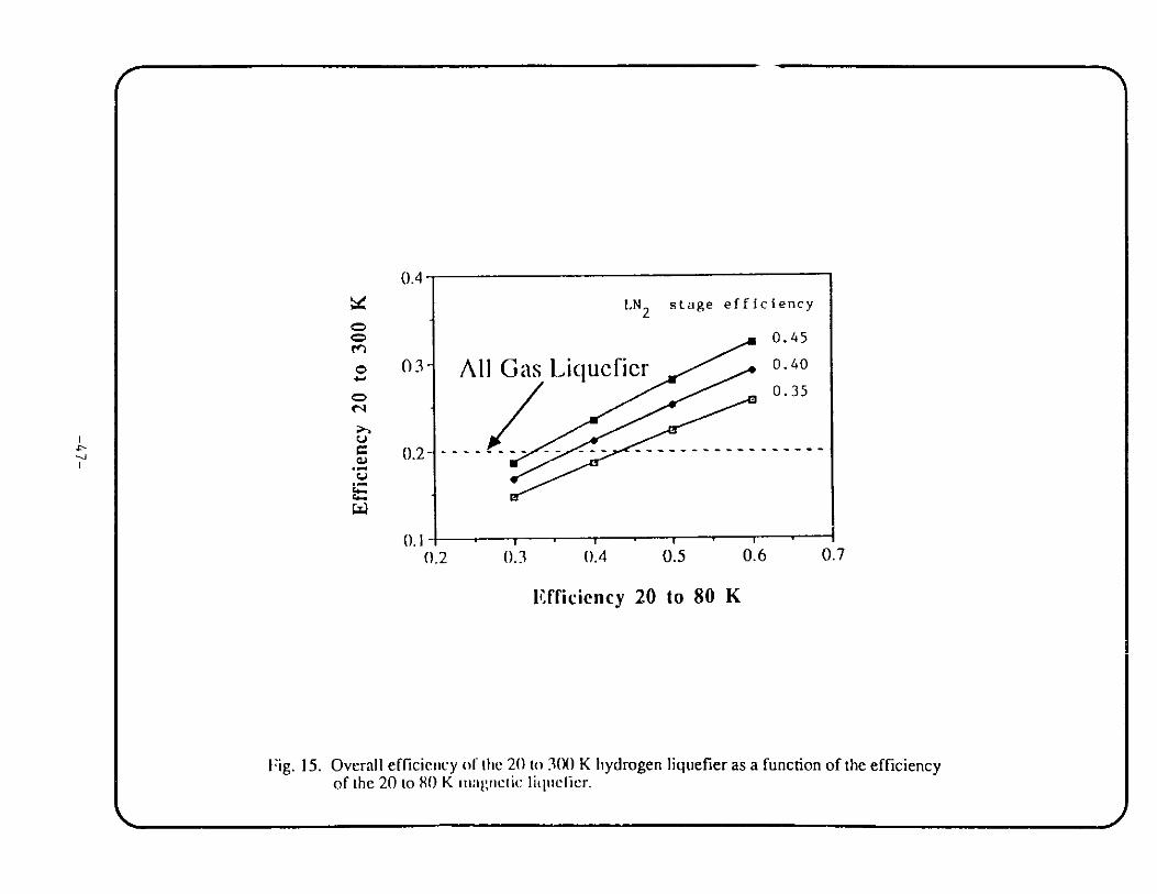
0.4

C>)

C>)

C>-

03

0.2-

0. 10.2 0.3 0.4 0.5 0.6 0.7

Efficiency 20 to 80 K

Fig. 15. Overall efficiency of the 20 to 3(X) K hydrogen liquefier as a function of the efficiencyof the 20 to 80 K inagnctic liquefier.

I

LN 2 stage efficiency

0.45

All Gas Liquefier 0.40

0.35

- - - - - - - - - - - - - - -

- --

or

--

T

%k% 000'M

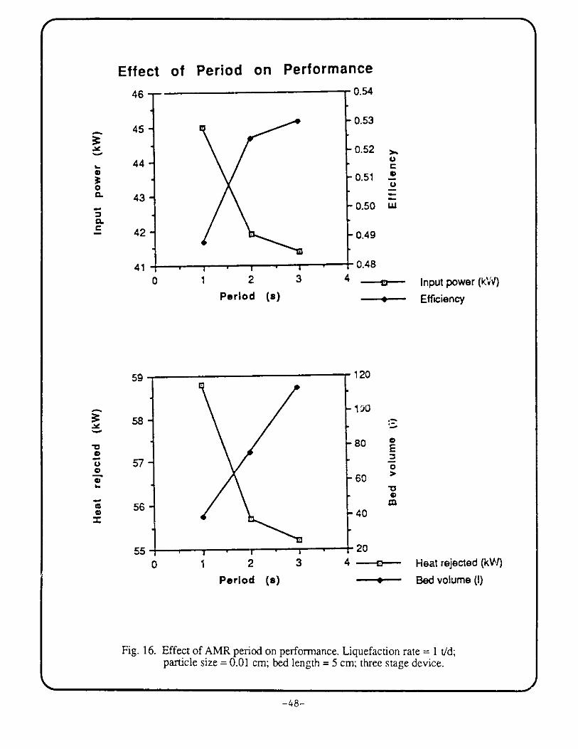
Effect of Period on Performance--

-F I

-U

1 2

Period (s)

3

0.54

0.53

0.52 ),

0.51 .!

0.50 w

0.49

'II

0.48

4 --.-- Input power (kW)----- Efficiency

S -- . .

2

Period (s)

120

-40o804 --

60 ~

20

40

3 Heat rejected (kW)

*+ Bed volume (I)

Fig. 16. Effect of AMR period on performance. Liquefaction rate = 1 t/d;particle size = 0.01 cm; bed length = 5 cm; three stage device.

-48-

46

45

44

43

42 -

0.

CL

410

59 -p 1"

58-

57-

56 -

%WO

O

V.

m

Goa

ccm

550 1

K9

Figure 17 illustrates the effect of field change on performance, or more accurately, the effect

of the adiabatic temperature change at 80 K of an ideal material on performance. As field increases,

the adiabatic temperature change increases. Assuming ErxGd(1-x)Al2 with a Curie point of 80 K for

the material at the hot end of the bed, the 9 K adiabatic temperature change corresponds to a field

change of approximately 7 to 8 Tesla. An adiabatic temperature change of 5 K corresponds to a

field change of about 5 T. These results come from mean field theory. From the results of Fig. 17, a

field change of 5 T would yield a device with too low an efficiency. A field change of 7 to 8 Tesla

is necessary to produce a competitive device from the standpoint of efficiency.

4.2.5 Scaling and Cost of AMR Liquefier

Several different magnetic refrigerator scaling analyses were performed in this study. All

involved a three-stage magnetic refrigerator for liquefying hydrogen, with 8 T superconducting

magnets, external heat exchangers, 0-P converters, and liquid nitrogen precooling of the incoming I

MPa (1 atm) hydrogen.

A rotary version of the AMR was chosen for the scaling and cost analyses but the

reciprocating design should not be regarded as unsuitable. The rotary AMR naturally produces

continuous cooling and uniform loads. It uses a wheel composed of many parallel particle beds in a

radial direction. The magnet remains stationary and the magnetic material continuously enters and

leaves the high-field region. Figure 11 illustrates the design. A high-field region is maintained by a

toroidal magnet configuration. In the high-field region, an radially outward flow is produced by

sliding seals on the inner and outer portion of the wheel. A housing surrounds the entire wheel so

these seals are only for small AP flow control purposes, not sealing to the vacuum in the cold box.

In the low-field region, similar manifolds and seals exist but the flow is radially inward.

In the first scaling analysis, the cost of a 1 t/d unit as a function of the wheel diameter was

studied. The recurring cost breakdown for a 145-cm mean diameter wheel is shown in Table VI

below. The cost varied by less than 3% for wheel diameters varying from 80 cm to 200 cm. In

calculating the recurring costs, material and labor ($10 /h direct) burden rates were assumed to be

100% and 200%, respectively. The analysis was done by taking each system component and

estimating the cost to the manufacturer based on our experience and from calls to vendors. The

source for each component is listed. Development costs have not been included.

-49-

4 5 6 7 8 9 1

Field Strength (T)

LC

POO

0.5 -- -- Input Power (kW)- - Efficiency

60

10

Field Strength (T)

Fig. 17. Effect of the field change on performance, expressed in terms of theadiabatic temperature change of the ideal magnetic material at 80 K.Liquefaction rate = 1 t/d; particle size = 0.01 cm; bed length = 5 cm.

J-50-

70

50

40

80

70

60

50 S 7 8 16 7 8 94 5

-.

\4,

I

7

0.4 -

-0.3

100 1teat Rejected (kW)* Bed Volume (I)

- 90

80 -

70

. 2

-50

- 40

30

-

-

1

-

r

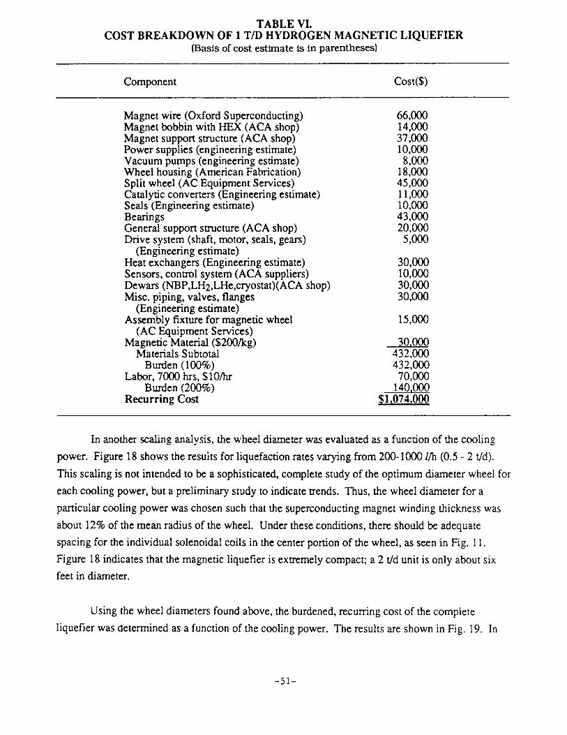
TABLE VI.COST BREAKDOWN OF 1 T/D HYDROGEN MAGNETIC LIQUEFIER

(Basis of cost estimate is in parentheses)

Component Cost($)

Magnet wire (Oxford Superconducting)Magnet bobbin with HEX (ACA shop)Magnet support structure (ACA shop)Power supplies (engineering estimate)Vacuum pumps (engineering estimate)Wheel housing (American Fabrication)Split wheel (AC Equipment Services)Catalytic converters (Engineering estimate)Seals (Engineering estimate)BearingsGeneral support structure (ACA shop)Drive system (shaft, motor, seals, gears)

(Engineering estimate)Heat exchangers (Engineering estimate)Sensors, control system (ACA suppliers)Dewars (NBP,LH2,LHe,cryostat)(ACA shop)Misc. piping, valves, flanges

(Engineering estimate)Assembly fixture for magnetic wheel

(AC Equipment Services)Magnetic Material ($200/kg)

Materials SubtotalBurden (100%)

Labor, 7000 hrs, 510/hrBurden (200%)

Recurring Cost

66,00014,00037,00010,000

8,00018,00045,00011,00010,00043,00020,000

5,000

30,00010,00030,00030,000

15,000

30,000432,000432,000

70,000140,000

$1,074.000

In another scaling analysis, the wheel diameter was evaluated as a function of the cooling

power. Figure 18 shows the results for liquefaction rates varying from 200-1000 1/h (0.5 - 2 t/d).

This scaling is not intended to be a sophisticated, complete study of the optimum diameter wheel for

each cooling power, but a preliminary study to indicate trends. Thus, the wheel diameter for a

particular cooling power was chosen such that the superconducting magnet winding thickness was

about 12% of the mean radius of the wheel. Under these conditions, there should be adequate

spacing for the individual solenoidal coils in the center portion of the wheel, as seen in Fig. 11.

Figure 18 indicates that the magnetic liquefier is extremely compact; a 2 t/d unit is only about six

feet in diameter.

Using the wheel diameters found above, the burdened, recurring cost of the complete

liquefier was determined as a function of the cooling power. The results are shown in Fig. 19. In

-51-

1 t/d200

r1

VN"MPOIL

r.+

GC

.. n

180-

160-

140-

120-

1 nnf

IU0 V I I

200 400 600 800 1000 1200

Liquefaction Rate (I/h)

Fig. 18. Mean wheel diameter versus liquefaction rate of magnetic hydrogen liquefier.

1 t/d

V:

Ew

1.8

1.6-

1.4-

1.2

1.0-

0.8-

0.6 2

200 400 600 800 1000

Liquefaction Rate (1/h)

1200

Fig. 19. Complete liquefier system cost as a function of liquefaction rate.

-52-

J

1

.t

this relatively simple analysis, the cost of the system appears linearly dependent on cooling power

over the range 0.5 - 2 t/d, such that

Cost = 0.001 X (Liq. Rate, 1/h) + 0.54 (19)

where cost is in millions of dollars and the liquefaction rate is in liters per hour. For example, the

cost of a I t/d or 533 1/h system is $1.07 M. This capital cost is much less than the projected cost for

a conventional gas cycle device. The smallest commercial hydrogen liquefier is a 5 t/d device

whose capital cost is about $12.5 M. If this cost is linearly extrapolated to a 1 t/d unit, it would cost

$2.5 M or more than twice the 1 t/d magnetic liquefier. A summary listing of the characteristics of a

1 t/d magnetic hydrogen liquefier is shown in Table VII.

TABLE VII.CHARACTERISTICS OF A 533 1/h (1 t/d) MAGNETIC HYDROGEN LIQUEFIER

Parameter Value

LH 2 Production RateStagesNominal Cold End Temperature

Stage 1Stage 2Stage 3

High-Temperature Heat SinkLN2 Boil-off RateMean Wheel DiameterWheel SpeedField StrengthMagnetic MaterialAmount of Magnetic MaterialInput Power (drive motor)Efficiency 80 K - 20 KOverall Efficiency 300 K - 20 K(assuming LN2 produced at 40%)

Estimated System Cost

533 l/h (1 t/d)3

60 K40 K20 KLN 2

1310 l/h (27.9 t/d)145 cm60 rpm

8TErxGdi -xAl2

152 kg45 k We

48%24%

$1,074,000

5. UPDATE OF ROOM-TEMPERATURE MHP REPORT

Astronautics Corporation of America completed a study entitled "Assessment of the Impact

of High Temperature Superconductors on Room Temperature Magnetic Heat Pumps/Refrigerators"

for ANL that was sponsored jointly by DOE's Office of Energy Conservation and Utilization

Technology (ECUT) and EPRI in July 1988 (Contract no. 81032401). This study took a "first look"

at the potential impact of high-temperature superconductors (HTSCs) on magnetic heat pumps

-53-

(MHPs). In particular, the study focused on both a heat pump absorbing energy from 350 K water

and delivering 500 kW to produce 389 K water, and an industrial refrigeration unit (supermarket

freezer) removing 50 kW from 255 K air and exhausting to 308 K air. Recuperative and

regenerative magnetic devices were analyzed.

Some of the conclusions from the room-temperature MHP study are reiterated below.

" Reliability is probably the most important criteria for selection of refrigerator or heat

pump equipment, although cost is a close second in importance.

" A 50-kW magnetic heat pump and refrigerator has been conceptually analyzed and

modeled to show performance comparable to, or better than, conventional vapor

compression devices.

" The active magnetic regenerator appears to have several advantages compared to the

magnetic recuperative design.

" The magnetic regenerator achieves high performance, i.e., large heat flux per kg, by

operating at higher frequency than earlier magnetic designs. (The frequency is well

below that of comparable regenerative gas-cycle refrigerators.)

" The capital and operating costs of the 50-kW magnetic devices has been estimated.

The capital costs appear larger than those of vapor-compression devices but the

operating costs are lower so an overall cost advantage appears after a few years.

" The costs of the magnetic units are a weaker function of size than for the vapor-

compression devices because similar magnets can be used for a variety of sizes.

" The magnetic heat pumps appear to be much more tolerable of variation in hot and

cold temperatures, which is generally not true for vapor compression devices.

" Magnetic units do not use chlorofluorocarbons.

One of the objectives of the present study is to update the ECUT/EPRI report based on the

results of this work. Although both studies involve MHP technology and both concentrate on rotary,

-54-

regenerator devices, there are significant differences which minimize the analysis overlap. The

supermarket refrigerator used:

" liquid (water plus ethanol) for heat transfer to the magnetic material (implies very

high heat transfer);

" parallel plates of magnetic material, gadolinium (implies ductile or malleable

material);

* porosity of 10% (high heat transfer); and

" the external medium to which heat is absorbed and rejected is a gas.

The hydrogen liquefier uses:

* helium gas for heat transfer to the magnetic material (relatively poor heat transfer);

" packed particle bed of magnetic material, ErxGd(1.x)Al2 (brittle material);

* porosity of 50% (about the lowest easily obtained porosity);

* the external medium to which heat is absorbed and rejected is mainly liquid.

Thus, the only practical area of overlap is in the costing analysis. The costing shown in

Table VII is more extensive than in the previous study. In many cases, costs have been verified by

outside vendors. The same analysis was applied to the 50-kW supermarket refrigerator. The total

materials cost is about 15% higher, but the estimated retail cost is almost twice that obtained

previously ($55 K now versus $26 K before). The new detailed cost breakdown with burdening

broken out is in Table VIII. Note that this breakout does not contain a magnet power supply or

vacuum pump because it was assumed that these would be used infrequently and therefore, supplied

by a servicing contract.

-55-

TABLE VIII.COST BREAKDOWN OF A 50 kW SUPERMARKET FREEZER

(Basis of cost estimate is in parenthesis)

Component Cost ($)

Magnet wire (Oxford Superconducting) 3,600Magnet bobbin with HEX (ACA shop) 1,200Magnet support structure (ACA shop) 400Wheel housing (American Fabrication) 1,400Split wheel (AC Equipment Services) 500Adiabatic material(Engineering estimate) 1,200Seals (Engineering estimate) 700Bearings 200General support structure (ACA shop) 500Drive system (shaft, motor, seals, gears) 500

(Engineering estimate)Manifolds (Engineering estimate) 500Sensors, control system (ACA suppliers) 1,000Dewars (NBP,LH 2 ,LHe,cryostat)(ACA shop) 2,000Misc. piping, valves, flanges 100

(Engineering estimate)Magnetic Material ($100/kg) 1,500

Materials Subtotal 15,300Burden (100%) 15,300

Labor, 800 hrs, $10/hr 8,000Burden (200%) 16,000

Recurring Cost $54,600

A number of factors contribute to this difference in retail costs. The previous analysis was

simplistic and brief. Retail costs were assumed to be twice the cost to the manufacturer.

Consultants indicated that a factor of three would not be unreasonable. Thus, the 555,000 retail cost

is probably now representative of the first cost of a 50kW magnetic supermarket freezer. This cost

should still be interpreted cautiously. A preliminary design of any real device is required to provide

vendors with drawings before a more accurate costing can be performed.

6. MAGNETIC REFRIGERATOR APPLICATIONS UP TO 300 K

One of the objectives of this study is to consider the application of a magnetic refrigerator

above 77 K. Although the liquefaction of numerous gases other than hydrogen could have been

considered, the scope of the project was limited by replacing the LN2 stage of the hydrogen liquefier

with a magnetic refrigerator. Table IX gives the specifications and performance of an AMR

operating between 77 and 300 K, computed using a zero-reduced-period AMR model. It is assumed

-56-

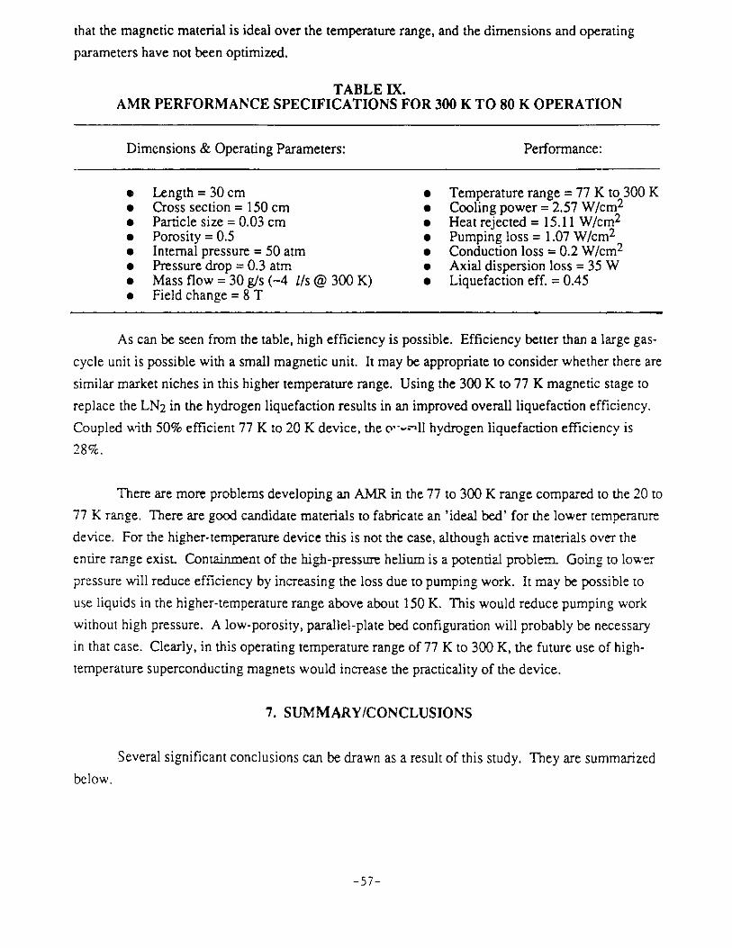
that the magnetic material is ideal over the temperature range, and the dimensions and operating

parameters have not been optimized.

TABLE IX.AMR PERFORMANCE SPECIFICATIONS FOR 300 K TO 80 K OPERATION

Dimensions & Operating Parameters: Performance:

" Length = 30 cm " Temperature range = 77 K to 300 K" Cross section = 150 cm * Cooling power = 2.57 W/cm2

" Particle size = 0.03 cm " Heat rejected = 15.11 W/cm2

" Porosity = 0.5 " Pumping loss = 1.07 W/cm2

" Internal pressure = 50 atm " Conduction loss = 0.2 W/cm 2

" Pressure drop = 0.3 atm * Axial dispersion loss = 35 W" Mass flow = 30 g/s (-4 l/s @ 300 K) " Liquefaction eff. = 0.45* Field change = 8 T

As can be seen from the table, high efficiency is possible. Efficiency better than a large gas-

cycle unit is possible with a small magnetic unit. It may be appropriate to consider whether there are

similar market niches in this higher temperature range. Using the 300 K to 77 K magnetic stage to

replace the LN2 in the hydrogen liquefaction results in an improved overall liquefaction efficiency.

Coupled with 50% efficient 77 K to 20 K device, the o' =1ll hydrogen liquefaction efficiency is

28%.

There are more problems developing an AMR in the 77 to 300 K range compared to the 20 to

77 K range. There are good candidate materials to fabricate an 'ideal bed' for the lower temperature

device. For the higher-temperature device this is not the case, although active materials over the

entire range exist. Containment of the high-pressure helium is a potential problem. Going to lower

pressure will reduce efficiency by increasing the loss due to pumping work. It may be possible to

use liquids in the higher-temperature range above about 150 K. This would reduce pumping work

without high pressure. A low-porosity, parallel-plate bed configuration will probably be necessary

in that case. Clearly, in this operating temperature range of 77 K to 300 K, the future use of high-

temperature superconducting magnets would increase the practicality of the device.

7. SUMMARY/CONCLUSIONS

Several significant conclusions can be drawn as a result of this study. They are summarized

below.

-57-

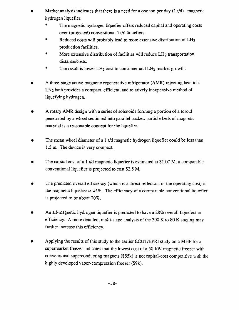
" Market analysis indicates that there is a need for a one ton per day (1 t/d) magnetic

hydrogen liquefier.

* The magnetic hydrogen liquefier offers reduced capital and operating costs

over (projected) conventional 1 t/d liquefiers.

* Reduced costs will probably lead to more extensive distribution of LH2

production facilities.

* More extensive distribution of facilities will reduce LH2 transportation

distance/costs.

* The result is lower LH2 cost to consumer and LH2 market growth.

" A three-stage active magnetic regenerative refrigerator (AMR) rejecting heat to a

LN2 bath provides a compact, efficient, and relatively inexpensive method of

liquefying hydrogen.

" A rotary AMR design with a series of solenoids forming a portion of a toroid

penetrated by a wheel sectioned into parallel packed-particle beds of magnetic

material is a reasonable concept for the liquefier.

* The mean wheel diameter of a I t/d magnetic hydrogen liquefier could be less than

1.5 m. The device is very compact.

" The capital cost of a 1 t/d magnetic liquefier is estimated at $1.07 M; a comparable

conventional liquefier is projected to cost $2.5 M.

" The predicted overall efficiency (which is a direct reflection of the operating cost) of

the magnetic liquefier i 24%. The efficiency of a comparable conventional liquefier

is projected to be about 0%.

" An all-magnetic hydrogen liquefier is predicted to have a 28% overall liquefaction

efficiency. A more detailed, multi-stage analysis of the 300 K to 80 K staging may

further increase this efficiency.

* Applying the results of this study to the earlier ECUT/EPRI study on a MHP for a

supermarket freezer indicates that the lowest cost of a 50-kW magnetic freezer with

conventional superconducting magnets ($55k) is not capital-cost competitive with the

highly developed vapor-compression freezer ($9k).

-58-

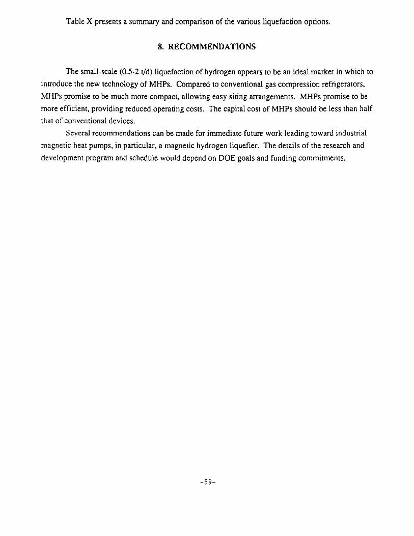
Table X presents a summary and comparison of the various liquefaction options.

8. RECOMMENDATIONS

The small-scale (0.5-2 t/d) liquefaction of hydrogen appears to be an ideal market in which to

introduce the new technology of MHPs. Compared to conventional gas compression refrigerators,

MHPs promise to be much more compact, allowing easy siting arrangements. MHPs promise to be

more efficient, providing reduced operating costs. The capital cost of MHPs should be less than half

that of conventional devices.

Several recommendations can be made for immediate future work leading toward industrial

magnetic heat pumps, in particular, a magnetic hydrogen liquefier. The details of the research and

development program and schedule would depend on DOE goals and funding commitments.

-59-

'TABLE X.

EFFICIENCY COMPARISON OF I TON PER IDAY A LL-GAS HYDROGEN LIQUEFIERS TO MAGNETIC LIQUEFIERCOMBINATIONS

TemlIerature Range& Technology

OverallLiquefaction rT

Relative EnergyUnit Mass of LH2

1 t/d all gashydrogen liquefier

27 t/d LN 2plant on-site+ AMR

27 t/d deliveredfrom a large LN2plant + AMR

All magnetic(future)

0'

(300 K - 2( K all gas)[I -').2()

(300 K - 77 K g ) + (77 K - 20 K AMR)Ti = 0.25 Ti = 0.49

(300 K - 77 K LN 2 hoiloff) + (77 K - 20 K AMR)TI = 0.40 TI = 0.49

(300 K -77 K AMR) + (77 K -20 K AMR)Ti= 0 .45 11= 0.49

*The efficiency of a 5 t/d 112 liquefier is 25% per Air Products,the 20% value is our estimate for a 1 t/d all-gas P-% liquefier

T = 0.20*

1 = 0.16

1.0

1.25

T = 0.25 0.8

i = 0.28 0.7

9. REFERENCES

1. J.A. Barclay and W. A. Steyert, Cryogenics, 2, 73 (1982). "Materials for MagneticRefrigeration Between 2 K and 20 K."

2. T. Hashimoto, et al,, Cryogenics, 21, 647 (1981). "Magnetic Refrigeration in theTemperature Range from 10 K to Room Temperature."

3. C.B. Zimm, et al., J. Apple. Phys., U, 2609 (1984). "Low Hysteresis Materials forMagnetic Refrigeration: Gd1-xErxAl2."

4. P. Weiss and A. Piccard, C.R. Acad. Sci. (Paris) , 352 (1918).

5. H.H. Potter, Proc. R. Soc. (London) 146, 326 (1934).

6. S.M. Benford and G.V. Brown, J. Apple. Phys., U, 2210 (1981). "T-S Diagram forGadolinium Near the Curie Temperature."

7. L. Brillouin and H.P. Iskenderian, Elec. Comm., 25, 300 (1948). "ThermomagneticGenerator."

8. J.F. Elliot, J. Apple. Phys., 3Q, 1774 (1959). "Thermomagnetic Generator."

9. L.D. Kirol and J.L. Mills, J. Appl. Phys., 5, 3 (1984). "Numerical Analysis ofThermomagnetic Generators."

10. D. Solomon, J. Apple. Phys., f&, 3687 (1989). "Thermomagnetic Mechanical HeatEngines."

11. S. Pappell, NASA Lewis Research Center (1965). U.S. Patent 3,215,572.

12. E.L. Resler and R.E. Rosenweig, J. Eng. Power, p. 399 (1967). "RegenerativeThermomagnetic Power."

13. E. Van Der Voort, Appl. Sci. Res., ?Q, 98 (1969). "Ideal Magnetocaloric Conversion."

14. J. Poppelwell and S. Charles, in Proceedings of Ferrofluid Conference entitledThermomechanics of Magnetic Fluids, edited by B. Berkowsky (Hemisphere PublishingCo., Washington, DC, 1978).

15. G.V. Brown, IEEE Trans. on Mag., MAG13, 1146 (1977). "Magnetic Stirling Cycles - ANew Application for Magnetic Materials."

16. G.V. Brown, J. Apple. Phys., 47, 3673 (1976). "Magnetic Heat Pumping Near RoomTemperature."

17. P. Debye, Ann. Phys., $., 1154 (1926). "Einize Burnerkungen zur Magnetisierung beitiefer Temperature."

18. W.F. Giauque, J. Am. Chem. Soc., 49, 1870 (1927) and W.F. Giauque and I.D.P.MacDougall, Physical Review, 4, 768 (1932). "Attainment of Temperatures Below 1 KAbsolute by Demagnetization of Gd2(SO4)3-8H2O)."

19. J.R. van Geuns, Philips Research Report Suppl. 6, (1966!. "A Study of a New MagneticRefrigerating Cycle."

-61-

REFERENCES(Continued)

20. J.A. Barclay, Adv. in Cryog. Eng., 2, 719 (1988). "Magnetic Refrigeration: A Review of aDeveloping Technology" and references therein.

21. A.F. Lacaze, Proc. Int'l Inst. of Refrigeration Conf., Prague, 1986, p. 99-110, "MagneticRefrigeration - An Overview."

22. T. Hashimoto, Adv. in Cryog. Eng., , 261 (1986). "Recent Investigations onRefrigerants for Magnetic Refrigerators."

23. L. D. Kirol and M.W. Dacus, Adv. in Cryog. Eng., 33 757 (1988). "Rotary RecuperativeMagnetic Heat Pump."

24. G. Patton, G. Green, J. Sevens, and J. Humphrey, Proc. 4th Int'l Cryocooler Conf.,Easton, MD, Sept. 25-26 (1986), "Reciprocating Magnetic Refrigerator."

25. J.A. Barclay and W.A. Steyert, Electric Power Research Institute (EPRI) Final ReportEL-1757, April, 1981. "Magnetic Refrigerator Development."

26. G.V. Brown, Am. Soc. of Heating, Refrigeration, and Air Conditioning Engineers Trans.,.Z, 783-793 (1981). "Basic Principles and Possible Configurations of Magnetic HeatPumps."

27. J.R Hull and K.L. Uherka, Proc. 23rd Intersociety Energy Conv. Engng. Conf., Denver,-, p. 531-536; July 31-Aug. 5 (1988); "Magnetic Heat Pumps."

28. 'Prrcwedings of the Magnetic Heat Pump Workshop," (P.E. Scheihing, editor), Oct. 27,1988, Herndon, VA; U.S. Dept. of Energy, Office of Industrial Programs.

29. The Market Potential for Electrolytic Hydrogen, Report prepared by the Futures Group,Glastonbury, CT, for the Electric Power Research Institute, EPRI Project No. 1086-4,Report No. EM-1154, Palo Alto, CA, August 1979.

30. Lee Gaumer, Air Products and Chemicals, Inc.; private communication (1989).

31. C.R Baker and RL. Shaner, Int. J. Hydrogen Energy, , 321 (1978). "A Study of theEfficiency of Hydrogen Liquefaction."

32. R. Barron, Cryogenic Systems. Oxford University Press (1985).

33. Cryogenic Engineering, edited by B.A. Hands, Academic Press (1986).

34. C.R. Cross, J.A. Barclay, A.J. DeGregoria, S.R. Jaeger, and J.W. Johnson, Adv. in Cryog.Eng., 2, 767, Plenum Press, New York (1988). "Optimal Temperature Entropy Curvesfor Magnetic Refrigeration."

35. J.A. Waynert, A.J. DeGregoria, S.R. Jaeger, J.W. Johnson, and J.A. Barclay, reportprepared by Astronautics Corp. of America for Argonne National Laboratory underDOE-ECUT/EPRI sponsorship (July 1988). "Assessment of the Impact of HighTemperature Superconductors on Room Temperature Magnetic HeatPumps/Refrigerators."

36. S. Whitaker, AICHE J., 18, 2 (1972). "Forced Convection Heat Transfer Correlations forFlow in Pipes, Past Flat Plates, Single Cylinders, Single Spheres, and for Flow inPacked Beds and Tube Bundles."

-62-

REFERENCES(Continued)

37. G.S.G. Beveridge and D.P. Haughey, Int. J. Heat & Mass Transfer, .j4. 1093-1113 (1971)."Axial Heat Transfer in Packed Beds: Stagnant Beds Between 20 and 750 C."

38. S. Sarangi and H.S. Baral, Cryog., 27 (1986). "Effects of Axial Conduction in the Fluidon Cryogenic Regenerator Performance."

39. I. F. Macdonald, et al., Ind. Eng. Chem. Fundam., .a, 199-208 (1979). "Flow ThroughPorous Media - the Ergun Equation Revisited."

40. W.R. Johanson, G. Pierce, C.B. Zimm, and J.A. Barclay, J. Appl. Phys., 4, 5892 (1988).

41. RD. McCarty, J. Hard, and H.M. Roder, NBS Monograph 168 (1981). "SelectedProperties of Hydrogen."

42. N.B. Vayaftik, Hemisphere Publishing (1975). "Tables on the ThermophysicalProperties of Liquids and Gases."

-63-