Martin Pfleiderer, Klaus Frieler, Jakob Abeßer, Wolf-Georg ...mainly jazz analysis, and in the...
352
Martin Pfleiderer, Klaus Frieler, Jakob Abeßer, Wolf-Georg Zaddach, Benjamin Burkhart (Eds.) Inside the Jazzomat New Perspectives for Jazz Research Veröffentlicht unter der Creative-Commons-Lizenz CC BY-NC-ND 4.0
Transcript of Martin Pfleiderer, Klaus Frieler, Jakob Abeßer, Wolf-Georg ...mainly jazz analysis, and in the...

Martin Pfleiderer, Klaus Frieler, Jakob Abeßer, Wolf-Georg Zaddach, Benjamin Burkhart (Eds.)
Inside the JazzomatNew Perspectives for Jazz Research
Veröffentlicht unter der Creative-Commons-Lizenz CC BY-NC-ND 4.0
978-3-95983-124-6 (Paperback)
978-3-95983-125-3 (Hardcover)
© 2017 Schott Music GmbH & Co. KG, Mainz
www.schott-campus.com
Cover: Portrait of Fats Navarro, Charlie Rouse, Ernie Henry and Tadd Dameron, New York, N.Y., between 1946 and 1948 (detail)
© William P. Gottlieb (Library of Congress)
Veröffentlicht unter der Creative-Commons-Lizenz
CC BY-NC-ND 4.0
The book was funded by the German Research Foundation
(research project „Melodisch-rhythmische Gestaltung von Jazzimprovisationen. Rechnerbasierte Musikanalyse
einstimmiger Jazzsoli“)

Martin Pfleiderer, Klaus Frieler, Jakob Abeßer, Wolf-Georg Zaddach, Benjamin Burkhart (Eds.)
Inside the Jazzomat
New Perspectives for Jazz Research


Contents
Acknowledgements 1
Intro
Introduction 5
Martin Pfleiderer
Head: Data and concepts
The Weimar Jazz Database 19
Martin Pfleiderer
Computational melody analysis 41
Klaus Frieler
Statistical feature selection: searching for musical style 85
Martin Pfleiderer and Jakob Abeßer
Score-informed audio analysis of jazz improvisation 97
Jakob Abeßer and Klaus Frieler
Solos: Case studies
Don Byas’s “Body and Soul” 133
Martin Pfleiderer
Mellow Miles? On the dramaturgy of Miles Davis’s “Airegin” 151
Benjamin Burkhart

ii
West Coast lyricists: Paul Desmond and Chet Baker 175Benjamin Burkhart
Trumpet giants: Freddie Hubbard and Woody Shaw 197Benjamin Burkhart
Michael Brecker’s “I Mean You” 211Wolf-Georg Zaddach
Right into the heart. Branford Marsalis and the blues“Housed from Edward” 227Wolf-Georg Zaddach
Bob Berg’s solo on “Angles” 243Klaus Frieler
Steve Coleman—Balanced improvisation 273Friederike Bartel
Following the red line: Chris Potter’s solo on “Pop Tune #1” 291Wolf-Georg Zaddach
Head out
Conclusion and outlook 305Martin Pfleiderer
Outro: Appendix
JazzTube: Linking the Weimar Jazz Database with YouTube 315Stefan Balke and Meinard Müller
The FlexQ algorithm 319Klaus Frieler
Brief introduction to circular statistics 323Klaus Frieler
Glossary 327
References 335

Acknowledgements
During the project runtime, a close and inspiring collaboration with severalpersons and institutions arose: The International Audio Laboratories Erlan-gen, in particular Meinard Müller, Stefan Balke, and Christian Dittmar, theSemantic Music Technologies group at Fraunhofer IDMT Ilmenau, namelyEstefanía Cano, and the Center of Jazz Studies and its J-DISC group, namelyTad Shull. Moreover, we would like to thank Andreas Kissenbeck, Munich,for inspiring exchanges about jazz theory, Wolfram Knauer, Jazz InstituteDarmstadt, for his continuous interest in our project, and Simon Dixon,Queen Mary University London, who initiated a successful application foran international two-year follow-up research project focused on pattern usagein jazz.
Most of the aforementioned persons came to Weimar to participate in one orboth of our International Jazzomat Research Workshops in September 2014and September 2016. We would like to thank all the participants, speakersand audience, of these workshops for sharing their time and taking part indiscussions about computational perspectives of jazz research with us.
Moreover, we extend our thanks to the Jazzomat community who testedpreliminary versions of our software and our database and gave invaluablefeedback, and to all the people who helped the project find a broader public.
A heartfelt thank you goes out to Christiane Kraft and Kerstin Höhn fromthe administration of the Music University Weimar, who helped manage theproject. We would also like to thank the German Research Foundation for thetwo grants which enabled both the existence of the project during 2012–2017and this publication in the first place and Nicola Heine for proofreading andrevising the manuscript.
Last but not least, cheers to all jazz musicians who provided us with thiswonderful music.
Weimar, June 2017
Martin Pfleiderer, Klaus Frieler, Jakob Abeßer,Wolf-Georg Zaddach, and Benjamin Burkhart


Intro


Introduction
Martin Pfleiderer
The Jazzomat Research Project is situated at the intersection between jazzresearch, music psychology and computational musicology. It aims at de-veloping new perspectives for jazz analysis as well as for the psychologyof improvisation and, last but not least, for computational music researchand music information retrieval (MIR). Up to now, the ongoing researchproject’s main contributions have been a database of 456 transcriptions ofmonophonic jazz improvisations (the Weimar Jazz Database) and a stand-alone software toolkit (MeloSpySuite/GUI) for the analysis of monophonicmusic; both of these, the database and software toolkit, are freely availableand open to further additions and adjustments by users. Several studies andnew approaches have been devised within the project both in the areas of jazzresearch and music psychology, e. g., the concept of midlevel units for analyz-ing jazz improvisations, resulting in a new model of improvisation, as wellas in music information retrieval, e. g., approaches involving score-informedautomated feature annotations of music recordings. The database and thesoftware as well as the project’s contributions to music information retrievalare introduced within the four chapters in the first part of this publication.The subsequent chapters within the second part of the book are devoted tonine analytical case studies using the Weimar Jazz Database and MeloSpyGUI.In this introductory chapter, the project’s background both in jazz research,mainly jazz analysis, and in the computer-aided analysis of music is outlined.Then, a brief overview over the book’s contents is given.
Jazz research: studying the infinite art of improvisation
The Jazzomat Research Project ties in with a long tradition of jazz researchwhich focuses on musicians and their performances, on creative processes

6 Martin Pfleiderer
and their cultural contexts. By introducing computational methods for theanalysis of recorded jazz improvisations the project aims at contributing tothis multifaceted research tradition with new analytical methods, a compre-hensive database and corresponding software tools.
Jazz is a musical performance practice which now spans over more thana century. The origins of jazz extend back to musical practices of AfricanAmericans living in New Orleans around 1900. In the 1920s, jazz increasinglygained recognition all over the United States and worldwide, culminatingin the swing craze of the late 1930s and early 1940s. In these times, jazzwas often viewed as a very popular musical practice for entertainment anddancing. However, since its beginnings, jazz has also striven for recognitionas an art form. During the 1940s, 1950s, and 1960s, both jazz musiciansand jazz critics strove for a cultural recognition of jazz. Modern jazz wasincreasingly appreciated in concerts and festivals as music one has to primarilylisten to ‘seriously’, and jazz critics such as André Hodeir (1956) or GuntherSchuller (1958) started to write about the artistic value of jazz music. Thiscritical writing involved an analytical approach to the music, relying stronglyon recordings and transcriptions. In particular, Schuller (1958) intended touse methods of music analysis to prove that a jazz musician, in this caseSonny Rollins with his improvisation on “Blue Seven” (1956), is at a similarartistic level to European composers. Later, Schuller wrote two extensivehistorical studies of traditional jazz and swing (Schuller, 1968, 1989) featuringcomprehensive analytical style portraits of leading musicians.
Since the late 1960s, the project of writing a history of jazz that is foundedin analytical scrutiny was pursued by jazz critics and musicologists withanalytical studies on jazz musicians such as Charlie Parker (Owens, 1974),Miles Davis (Kerschbaumer, 1978), Lester Young (Porter, 1985), or JohnColtrane (Putschögl, 1993; Porter, 1998). Moreover, Thomas Owens (1995)adopted Schuller’s approach of an analytical style history with regard tomodern jazz styles (bebop, cool jazz, hardbop). His rather sketchy styleportraits were complemented by many other studies, e. g., Bickl’s study ofseveral bebop musicians (Bickl, 2000). Ekkehard Jost (1975) presented anextensive study of the creative principles guiding free jazz or avant-garde jazzmusicians of the 1960s by analyzing the music of, among others, OrnetteColeman, Cecil Taylor, and the late John Coltrane.
In general, the analysis of the creative principles that guide jazz improvisationrelies strongly on recordings. However, it is questionable to study a recordedimprovisation as a final musical work even if it results from a longer chainof rehearsals and preliminary recordings which could be conceived as draftversions (Tirro, 1974). On the contrary, the art of jazz could be termed an

Introduction 7
“infinite art of improvisation”, as the subtitle of Paul Berliner’s seminal studystates (Berliner, 1994), one that does not find its objective in an ultimateperformance or recording of a piece. Ekkehard Jost argues for a methodologyof jazz analysis that aims at describing the prevailing creative principles of anindividual style of improvisation rather than certain musical artifacts:
How relevant is an analysis of recorded improvisations made on acertain date and under certain circumstances (the group involved,the improviser’s physical and mental disposition, the conditionsimposed by the producer, etc.)? This will depend on the extent towhich those improvisations can be taken, beyond the immediatemusical facts, as indicative of the specific musicians’ and groups’creative principles. (. . . ) analysing and interpreting the featuresof a given improvisation demands that the analyst take (sic!) intoaccount everything he has learned from other improvisations bythe same musician. The significance of general pronouncementson the stylistic features of an improviser, from whom one hasjust a single solo at hand, is minimal, while the likelihood ofdrawing false conclusions is very great (Jost, 1975, p. 13f.).
This suggests a two-step methodology of jazz analysis: First, listen to theavailable recordings of a musician or a group. Then, choose the pieces thatseems to be typical for the creative principles of the respective musician andanalyze them in detail in order to pinpoint and depict those principles.
John Brownell (1994) emphasizes that jazz unfolds dynamically within aperformance process which involves instantaneous improvisation as well asinteraction between the musicians. Therefore, he differentiates between theanalysis of those unfolding processes and an analysis of the results, such ascommercial recordings. Focusing on improvisation as a process opens upan interdisciplinary field of investigation involving approaches and method-ologies taken from ethnomusicology, sociology and music psychology. Thisinvolves interviews with musicians (Berliner, 1994; Monson, 1996; Norgaard,2008; C. Müller, 2017), participatory observation in the recording studios andat club stages (Jackson, 2012), and introspection (Sudnow, 1999). Notably,many of these scientific approaches to jazz improvisation also involve ananalytical study of recordings and their transcriptions. For instance, at leastone third of Berliner’s ethnographic study Thinking in Jazz (1994) is devotedto music examples transcribed from jazz recordings and to their analyticalexploration.
Following the ideas put forth by André Hodeir and Gunther Schuller, BarryKernfeld (Kernfeld, 2002b, 1995, p. 119-158) proposes different types of im-

8 Martin Pfleiderer
provisation. In paraphrase improvisation, prevalent in jazz of the 1920s and1930s, a musician refers closely to the original melody of a piece, ornamenting,varying or reworking it. By contrast, in so-called chorus phrase improvisation,jazz musicians improvise without much reference to a tune’s theme, insteadinventing new lines that fit the harmonies of the original composition. Often,this strategy relies on a vocabulary of formulas, patterns or ‘licks’ which areartfully woven into ever-changing melodic lines (formulaic improvisation).The usage of repeated patterns during improvisation has become one of themain issues in the study of jazz improvisation and is thoroughly discussed byOwens (1974, 1995), Smith (1991), Berliner (1994), and Finkelman (1997). Inmotivic improvisation, the musicians vary one or several motives, sometimestaken from the theme of a piece, but more often drawn from the ongoingstream of improvisational ideas, with strategies such as ornamentation, trans-position, rhythmic displacement, expansion, compression etc. In particular,this type of improvisation flourished within modal jazz, avant-garde jazz andfusion music, since in those styles the musician is for the most part free fromrapidly changing chords.
Besides these improvisation strategies identified by Kernfeld, there are severalfurther dimensions and creative principles to be investigated in improvisedjazz music. These are, first of all, the tonal and harmonic implications ofimprovised melodic lines as well as their relation to the original melodyand the chords they are based on and, secondly, the rhythmic features ofthe improvised lines, including particular features such as cross rhythms ormicro-rhythmic play that contribute to the overall ‘feel’, ‘swing’ or ‘drive’of a solo (see e. g., Friberg & Sundström, 2002). While for a long time ana-lytical jazz studies focused on the improvising soloists alone, Berliner (1994)and Monson (1996) presented transcriptions and analyses of a whole jazzgroup playing together. This, thirdly, opens up perspectives on the interactiveprocesses between musicians. Robert Hodson (2007) and Benjamin Givan(2016) continued to systematically explore the interplay both between thesoloist and rhythm section and within the rhythm section. Last but not least,the individual instrumental or vocal ‘sound’ characterizes the style of a jazzmusician. All of these features contribute to the overall dramaturgy of ajazz improvisation, often described by metaphors such as “telling a story”,“making a journey” or “doing a conversation” (see Berliner, 1994; Bjerstedt,2014), its aesthetic coherence and complexity or simplicity, as well as to thestylistic conciseness and recognizability of a musician or style.
While there are countless studies on the leading jazz musicians of the 1940sand 1950s, approaches to postbop avant-garde and fusion music are still ratherscarce. Besides Jost’s seminal research on free jazz both in the United Statesand in Europe (Jost, 1975, 1987), e. g., Keith Waters (2011) examined the

Introduction 9
recordings of Miles Davis’ 1960s quintet, and Andrew Sugg compared impro-visational strategies of saxophone players John Coltrane, Dave Liebman, andJerry Bergonzi (Sugg, 2014).
Since the late 1960s, the growth of jazz studies was paralleled by a growingdemand for jazz education and jazz theory, both in the United States andin Europe, and resulted in a consolidation or even canonization of jazzhistory for students’ textbooks. However, since the 1990s, a critique of thatcanon and new approaches to jazz studies have been promoted by severalresearchers from various disciplines, namely by film scholar Krin Gabbard(1995a, 1995b, 1996) and literary scholar Robert O’Meally (2004; 2007). Bothof them looked for relationships between jazz and American cultural history,e. g., by inquiring into the contribution made by jazz critics to the historyof jazz, or the intersections between jazz music and other art forms such asliterature, film, photography, and painting. This approach was labeled “newjazz studies” (cf. O’Meally et al., 2004) to set it apart from the ‘old’ jazz studiespursued by jazz critics and musicologists, who investigated jazz primarilyas an art form and sometimes detached from its cultural meanings and thesocial conditions of production and reception. However, in ‘new jazz studies’,the music itself often tends to be faded out altogether and in this regardits approach often falls behind the efforts of jazz analysis to appreciate thesounding dimensions of jazz performances. Surprisingly, many studies in theanthologies edited by Gabbard and O’Meally are dedicated to the Americanjazz canon from 1940s bebop to 1960s avant-garde jazz, while minor figuresas well as the somewhat confusing varieties of both jazz after 1980 and jazzoutside the United States tend to be neglected.
To sum up, there are several approaches to studying jazz improvisation, allof which complement each other and in doing so, deepen and enrich theunderstanding, aesthetic pleasure and appreciation of the music as well asan interpretation of its meaning within its cultural and social context. TheJazzomat Research Project aims at contributing to these approaches withboth a repository of several hundreds of high-quality transcriptions andcomputer-based methods. The transcriptions were manually annotated byjazz experts with the aid of computer software using a newly developed dataformat. Furthermore, a software toolkit was developed to meet the mani-fold requirements of an analytical approach to monophonic lines, e. g., theexamination of pitches and their harmonic implications, duration, rhythmand micro-rhythm, as well as the usage of patterns. These achievements werepossible thanks to the close collaboration of software engineers with both aninterest in music research and an understanding of jazz on the one hand, andjazz researchers open to concepts and procedures from computational musicanaylsis and music information retrieval on the other.

10 Martin Pfleiderer
Computational music analysis
The Jazzomat Research Project is rooted in a longer tradition of computa-tional musicology and aims to contribute to that growing field of research—within and beyond jazz music. Computational musicology started withinethnomusicology where researchers often collected, annotated and examinedlarge repositories of music recordings and manual transcriptions. Computershelped to handle these collections, e. g., by systematically managing the meta-data and manual annotations (Bronson, 1949; Lomax, 1976) and enablingautomated inquiries into those data. An important step towards computa-tional music analysis was the introduction of machine-readable formats forsheet music. Besides widespread music formats such as MIDI (since 1982),several formats were developed for scientific purposes, e. g., the Essen As-sociative Code (EsAC), designed for building and analyzing the Essen FolkSong Collection, and the **kern-format. Since the 1990s, David Huron andothers have encoded large amounts of sheet music in the **kern-format(Huron, 1999; Cook, 2004), including the Essen Folk Song Collection andmany scores of classical European as well as non-Western music. Recently,Temperley and de Clerq designed a new format for their transcriptions ofrock songs (Temperley & DeClercq, 2013; DeClercq & Temperley, 2011).According to Nicholas Cook, these new music databases
present a significant opportunity for disciplinary renewal: [...]there is potential for musicology to be pursued as a more data-rich discipline than has generally been the case up to now, andthis in turn entails a re-evaluation of the comparative method(Cook, 2004, p. 103).
Huron and collaborators developed a modular software toolkit, the Hum-drum Toolkit, which enables a flexible analysis of various features encodedin **kern-format. Further modular analysis toolkits are the MIDI-Toolbox(Eerola & Toiviainen, 2004), which works within the MATLAB environment,and the music21 library for Python (Cuthbert & Ariza, 2010). All of thesesoftware tools have their merits and downsides of course; their helpfulness forjazz research appears to be rather limited. By contrast, the software toolkitMeloSpySuite/GUI for Windows and OS X was designed especially for theanalysis of monophonic melodic lines and has several specific functionalitiesfor jazz improvisations.
In general, computer-aided music analysis has many advantages. Computersare able to extract musical features quickly, accurately and automatically fromlarge amounts of data, such as an improvisation encompassing hundreds orthousands of tone events, and repositories of thousands of folk songs or jazz

Introduction 11
improvisations. The feature extraction results in representations (e. g., tables,graphs, statistical values) of the music in regard to various musical dimensionsand creative principles, e. g., histograms of pitch class occurrence throughouta music piece or statistical values concerning its degree of syncopicity orchromaticity. As Cook puts it,
[t]he value of objective representations of music, in short, liesprincipally in the possibility of comparing them and so identify-ing significant features, and of using computational techniquesto carry out such comparisons speedily and accurately (Cook,2004, p. 109).
Comparison is a central capacity of the human mind and an importantoperation in science. To compare two or more objects, one has to identifysome common feature dimensions; if they had nothing in common, onewould be comparing apples and oranges. Several objects can then be comparedin regard to their similarities along these feature dimensions. The researcher’stask is to choose suitable feature dimensions based on research objectives.The computer algorithms can then be used in order to extract the chosenfeatures objectively and, in many cases, also more quickly and reliably. In anycase, clear and explicit analytical terminology that can be unambiguouslytransformed into algorithms and data structures is a prerequisite of computer-aided analysis routines. At times, this can help clarify fuzzy ‘traditional’terminology, which is a welcome side-effect.
Besides comparing pieces and identifying their significant features, computer-generated representations could also be used in a more explorative manner—asa kind of guidance leading the researcher to listen to particular features thathad hitherto passed unnoticed. However, it is important to emphasize thatthese computational tools and facilities are not meant to (and are hardly ableto) replace human researchers, but are for the most part designed for thepurpose of enriching traditional methodologies. Since music analysis alwaysinvolves individual processes of learning and understanding, a researcher hasto listen closely to the music in the first place and then identify its typicaland idiosyncratic features (cf. Cook, 2004, p. 107). However, this processof ‘close listening’ to certain pieces could be enhanced and stimulated by akind of ‘distant listening’ enabled by algorithms and software tools. Onemain intention of the analytical case studies presented in the second part ofthis book is to demonstrate how the analysis of certain typical or particularexamples can be fruitfully combined with computer-aided ‘distant listening’to larger repertoires and how these latter routines could support and extendan understanding of the music.

12 Martin Pfleiderer
Inside the Jazzomat: an overview
This book is an interim report on the ongoing Jazzomat Research Project,focusing mainly on its contributions to jazz research and jazz analysis. In itsfirst part, several basic assumptions and concepts of the project are introduced.In the following chapter the Weimar Jazz Database is introduced, includingthe transcription process, the assets and drawbacks of the data format as wellas the criteria for data selection. Additionally, the contents of the WeimarJazz Database (release version 2.0) and some of its features and peculiaritiesare outlined.
Then, the basics of computational melody analysis are discussed—whichare at the core of the MeloSpySuite/GUI software. With the aid of thisstand-alone software, various musical features of several musical dimensionscan be extracted from the transcription data. The mathematical conceptsof music representation, segmentation and annotation, feature extractionand pattern mining are introduced along with several examples. Includedare short introductions into the approach to a metrical quantification of thedata, the concept of midlevel annotation, descriptions of the most importantof those features available in MeloSpySuite/GUI as well as the approach topattern search with regular expressions.
In the subsequent chapter, a statistical approach to the characterization andanalysis of musical style is depicted. By using a subset of the musical featuresextracted by MeloSpySuite/GUI as well as subsets of the Weimar Jazz Data-base, one can explore which musical features distinguish a certain subset ofimprovisations, e. g., all improvisations by a certain musician or in a certainjazz style, from the remaining improvisations of the database. The potentialsof this powerful and promising statistical approach are exemplified in regardto several subsets and research issues.
While the Jazzomat Research Project focuses on symbolic data, i.e., transcrip-tions of recorded jazz improvisations, there are several additional aspectsconcerning an exploration of the audio recordings. Therefore, in the last chap-ter of the first part, several approaches to linking symbolic and audio datausing state-of-the-art algorithms are introduced. At first, approaches basedon a score-informed source separation between soloing and accompanyinginstruments are depicted. This approach leads to an automatic assessmentof instrument tuning, tone intensity and tone-wise pitch contour tracking.Furthermore, approaches to an analysis of instrument timbre (as a centralaspect within the personal sound of a jazz musician) and an approach toan automatic beat-wise transcription of walking bass lines with deep neuralnetworks are introduced. Additionally, several findings that rely on thesenew approaches and the data of the Weimar Jazz Database are depicted.
Introduction 13
The second part of the book encompasses nine analytical case studies whichcan also be read as examples of how to research on jazz improvisation eitherwith statistical methods and computational analysis tools or with more con-ventional analytical methods—or with a combination of both approaches. Bydemonstrating some of these possibilities, the case studies aim at stimulatingfurther analytical research with both the transcriptions included within theWeimar Jazz Database and the MeloSpySuite/GUI software. The main chal-lenge is to meaningfully relate insights gained from closely listening to themusic and from its close description with more abstract musical features andrepresentations that can be generated automatically by the software. Eachchapter focuses on certain issues exemplified by the analysis of one or moreparticular improvisations. In most cases, these analytical findings are contex-tualized within a larger stylistic context-—be it within the context of otherimprovisations by the same musicians or other musicians, or within a largerrepertoire of recordings. The comprehensive aim of these analytical case stud-ies is to open up new perspectives for analytical jazz research by combiningthe advantages of old-school jazz analysis with an analysis supplemented bycomputer-based methods and comparative approaches.
The first case study is dedicated to two improvisations on “Body and Soul”—one of the jazz standards most favored by jazz musicians. While ColemanHawkins’s recording of “Body and Soul” (1939) is widely appreciated as animportant and influential milestone in the history of jazz improvisation, thefocus is at first placed on the improvisation by a minor figure in jazz history,Don Byas, who recorded “Body and Soul” in 1944. Then, features of theimprovisations by Byas and Hawkins are compared with each other and, indoing so, Gunther Schuller’s characterization of an overall intensificationprocess within Hawkins’s solo (Schuller, 1989, p. 444) is re-examined bystatistical means.
Trumpet player Miles Davis is said to have established a less formulaic andinstead more melodic and motivic style of improvisation. In the case studyon Davis’s improvisation on “Airegin” (1954), presumably one of the firsthardbop recordings, several features of Davis’s ‘mellow’ style are character-ized, especially in regard to both the usage of different categories of midlevelunits and the overall dramaturgy of the improvisation. Additionally, Davis’ssolo is compared with both improvisations by several bebop trumpeters andother improvisations by Davis.
While Davis is a pivotal figure within the history of modern jazz and hasbeen discussed in many books and articles, there are legions of jazz musicianswho have been rather neglected by jazz analysis so far. Moreover, jazz stylessuch as West Coast jazz or postbop have only been tentatively explored by
14 Martin Pfleiderer
jazz research up until today. In West Coast lyricists the styles of trumpeterChet Baker and alto saxophonist Paul Desmond, which are often describedas ‘lyrical’, are characterized and compared with those of other cool jazzand West Coast jazz musicians included in the Weimar Jazz Database. Thecase study aims both at exploring characteristics associated with Baker andDesmond as well as with West Coast jazz in general and at providing afoundation for further analytical research.
The remaining six case studies are dedicated to important musicians who areusually attributed to postbop style. Postbop musicians seem to be very influ-ential for young jazz musicians and improvisation techniques developed bythem are at the very core of more recent trends in jazz education (Kissenbeck,2007). However, there is still a gap concerning an analytical, comprehensivecharacterization of improvisation strategies in postbop. The case studies aimat contributing to fill this gap. At first, two influential postbop trumpeters,Freddie Hubbard and Woody Shaw, are examined in regard to two aspectswhich seem to be characteristic for their personal style of improvisation: theusage of uncommon interval leaps within the fast lines played by both ofthem and the usage of recurring patterns, especially within Hubbard’s soloon “Maiden Voyage” (1965) and Shaw’s solo on “In a Capricornian Way”(1978).
Tenor saxophonist Michael Brecker is one of the most influential postbopmusicians. His playing style could be characterized as a virtuosic explorationof several improvisation techniques, including temporarily playing ‘outside’the chord changes or tonality. As is shown in the analytical case study ofhis improvisation on Thelonious Monk’s “I Mean You” (1995), however, hisinventive personal style is rooted in the jazz tradition and alludes to severalmore conventional strategies of improvisation. The relation between postbopplaying and the jazz tradition is analyzed in an analytical case study of a soloplayed by tenor saxophonist Branford Marsalis in the trio recording “Housefrom Edward” (1988). Again, the question of how different strategies ofimprovisation contribute to the overall dramaturgy of the piece is discussed.
While the case studies on Brecker and Marsalis are conceived as both a closeanalytical description of the particularities of a certain improvisation and aquestioning and contextualizing of more conventional analytical tools basedon jazz theory, the case study on tenor saxophonist Bob Berg’s solo on“Angles” (1993) takes a slightly different approach. The dramaturgy of thesolo is exhaustively explored in regard to many of the features that could beextracted by the MeloSpyGUI software, including midlevel units and patternusage, and then contextualized within the repertoire of the whole WeimarJazz Database. This statistical contextualization aims at answering one central

Introduction 15
question of jazz analysis: Which musical aspects and which creative strategiesdifferentiate a certain improvisation from other improvisations?
Steve Coleman stands out from various other postbop saxophonists in regardto his idiosyncratic concept of tonality which he has described as “symmet-rical movement”. Taking his solo in “Pass It On” (1991), it is asked whichtraces of this guiding principle can be found within Coleman’s improvisationsand how the tonal and rhythmical dimension of his playing style might becharacterized in general. This includes a comparison with another solo byColeman as well as with two solos on “Pass It On” played by other musicians.
The analytical part of the book is concluded by a case study of a solo bysaxophone player Chris Potter, who is one of the most widely appreciated jazzmusicians of a younger generation born after 1970. His solo on “Pop Tune#1”, recorded live in 2007, is a striking example of his distinctive personalstyle, which both emphasizes rhythmical improvisation orientated towardsgroove-based popular music and includes advanced strategies of ‘outside’playing.
The book closes with a summary and a critical discussion of the findings, andleads to conclusions in regard to new perspectives and possibilities as well aschallenges and tasks opened up for jazz research, both by transcriptions in adata format readable by computer and by software tools for music analysis,such as the MeloSpyGUI. In the appendix, there are condensed introductionsinto the the concept of JazzTube, the FlexQ algorithm and circular statis-tics, a glossary of technical terms from jazz theory, music analysis, statisticsand music information retrieval as well as a bibliography of cited works.Discographical information in regard to the analysed recordings as well as acomprehensive documentation and tutorials of both the Weimar Jazz Data-base and MeloSpyGUI are available at the website of the Jazzomat ResearchProject.1
1http://jazzomat.hfm-weimar.de


Head: Data andconcepts


The Weimar Jazz Database
Martin Pfleiderer
In this chapter, the Weimar Jazz Database is described. Concepts and purposesof the transcriptions and the data format are presented in detail and thetranscription process is outlined. Furthermore, the criteria for the selectionof jazz solos are discussed. Finally, the database content and some of itspeculiarities are portrayed.
Transcription and data format
The art of jazz improvisation is elusive and hard to grasp. However, audiorecordings offer an opportunity to reproduce the sounding dimension ofimprovised performances, to listen to them repeatedly and to study themin detail. Transcriptions, i. e., visual representations of what one hears andcomprehends while listening to music, are of great help for musical analysis.They allow for comparisons both between temporally distant passages withina performance and between different improvisations by one musician ormany musicians.
Therefore, it is not surprising that the use of transcriptions of audio recordingsis widespread in jazz research as well as in jazz education. While transcribingmusical details, the listener becomes more familiar or even intimate with themusic—leading to a deepening of his or her knowledge and understandingof the music (cf. Winkler, 1997). Many transcriptions of jazz solos can serveboth as an analytical description of music structures and processes as well as aprescription—or used less rigidly, as inspiration—for performance and impro-visation and therefore lie somewhere on a continuum between descriptiveand prescriptive music notation (cf. Seeger, 1958; Rusch, Salley, & Stover,2016). On the one hand, there are countless prescriptive transcriptions ofjazz solos that serve as the basis for a re-performance by younger musicians.

20 Martin Pfleiderer
This is a common learning strategy for enhancing and enlarging one’s ownimprovising skills and for learning about the improvisational strategies ofthe older generation (see Berliner, 1994). Therefore, building on a set ofhandy conventions within the jazz community, e. g., in regard to the nota-tion of swinging eighths, prescriptive transcriptions should be easy to read.Descriptive transcriptions, on the other hand, are made by scholars in orderto analyze certain stylistic features or aesthetic peculiarities of a performance.While these analytical transcriptions tend to be more detailed, every tran-scription is a compromise situated between the poles of easy readability anda precise representation of musical details.
Within the field of jazz research, there are various analytical strategies. Onecould be interested, e. g., in the examination of and comparison betweenmelodic dramaturgies, harmonic strategies, pattern usage, interaction pro-cesses, micro-rhythmic peculiarities or expressive qualities. The notationalsystem used in a transcription can vary substantially with regard to style andthe amount of detail, depending on these various analytical objectives. Thus,descriptive music transcription in general is hardly separable from both theanalytical issues at stake and from an interpretation of analytical findings(Owens, 2002; Rusch et al., 2016, p. 293).
The aim of the Weimar Jazz Database is to meet the requirements for asmany analytical issues as possible. What is actually annotated manually arepitches and their durations (onset and offset time), chord changes, beat andmeter, form sections, phrase boundaries as well as some expressive features.Additionally, information regarding the dynamics and the intonation of thetones played is extracted automatically, as are accompanying bass lines. Lastbut not least, annotations of so-called midlevel units are included for all solos(cf. Chapter Computational melody analysis). The annotation of midlevel unitsfollows a new qualitative approach introduced by Frieler et al. (2016a) toexamine improvisational processes. Therefore, scholars interested in creativeprocesses, jazz theorists interested in harmonic strategies and jazz historianswho follow stylistic differences in regard to dramaturgy, melody or rhythmand micro-rhythm can all benefit from the transcriptions within the WeimarJazz Database.
Unfortunately, due to temporal resources, it was not possible to transcribeall the information in a recorded solo. First of all, the database is restrictedto monophonic improvisations. Although it would be desirable to includepolyphonic solos played, e. g., on the piano, guitar or vibraphone, thesetranscriptions would be quite laborious to produce. However, a few single-line solos played on the piano, guitar and vibraphone are included. Secondly,each transcription includes only the melodic line of one improvising soloist

The Weimar Jazz Database 21
and does not refer to the full accompaniment of the rhythm section or theinterplay between several musicians. The transcription of a whole group(cf. Berliner, 1994; Hodson, 2007; Waters, 2011; Givan, 2016) was beyondthe scope of our project. However, the melodic lines were placed within themetric and harmonic framework of the performance and beat-wise pitchestimates of the accompanying bass lines were added. Thirdly, features of thesounds actually played by a musician, their timbre, dynamics and intonationas well as expressive features such as ghosted notes, vibrato etc. are crucialfor the particular rendition of a melodic line and for the overall style ofa jazz musician. However, it is hard to transcribe these features reliably.Therefore, vibrato, slides etc. are only roughly described using verbal tags,while dynamics and intonation are extracted automatically by advanced audioalgorithms.
The improvised solos were transcribed manually by a team of students and su-pervised by one of the editors (Wolf-Georg Zaddach). While there are severalautomatic transcription programs available today (e. g., Songs2see, Tony),none of them met our purposes. The results of these automatic transcriptionsoftware are quite inaccurate, so that a correction of the faulty output ap-peared to be more laborious than transcribing from scratch. However, theSonic Visualiser2 software proved to be a helpful tool for the transcriptionprocess. Sonic Visualiser is a powerful and easy-to-handle tool for the visualiza-tion of various aspects of an audio-file. Its main concept is the non-destructivesuperposition of annotation or visualization layers or panes. Sonic Visualiserallows for
• transcribing notes in a piano-roll-like notation that is easily generatedin a note layer;
• tapping along with the recording in order to generate a beat grid in atime-instant layer;
• adding chords and section names (e. g., chorus 1 or secetion A, B etc.)to the beats in an editor window;
• adding further region and text layers in which phrases and expressivecharacteristics (slides, vibrato, bends etc.) can be captured;
• monitoring the transcription in parallel with listening to the recording;
• slowing down the recording speed while listening to it in order toidentify details;
2http://www.sonicvisualiser.org/

22 Martin Pfleiderer
• visual support during the transcription process with a spectrogramlayer.
The staff members involved in the transcription process relied heavily onthese features. For each solo, they used a note layer to notate the pitch, onset,and offset of the tones. They did not have to assign metric starting points ornote values to the tones—one of the more intriguing aspects of transcriptionwhich is often open to a certain amount of ambiguity and interpretation (seeRusch et al., 2016). Since automatic beat and bar detection algorithms—whichwere integrated in the Sonic Visualiser software via Vamp Plugins—provedto be not very reliable in the case of jazz, we settled on manual tapping in atime-instant layer for beat annotation. To this beat track, metric information,chords and form sections were added manually. In general, annotated chordswere taken from available lead sheets (mainly various issues of Realbooksand Aebersold recordings) and were added in the same manner throughoutall the choruses during a solo. In some cases, chords taken from lead sheetswere modified to correspond to the chords actually played by the rhythmsection. Musical phrases were annotated in a region layer according to theperception and judgment of the transcriber. Additionally, bass pitches perbeats, e. g., the pitch of the walking bass line, dynamics of the solo tones aswell as aspects of intonation were added automatically to the transcriptions.
The structure of the transcription process and the resulting transcription datais depicted in Figure 1. The annotations can be exported in Sonic Visualiserproject files (with the file extension .sv), which are the basis for the database.Additionally, various metadata concerning the solo, the recording, and thetranscription were collected in an Excel spreadsheet, the so-called mastertable. The metadata can be partially inspected and exported for analyticalpurposes with MeloSpyGUI. A short introduction into the database formatand into some manually annotated metadata categories (such as style, genre,rhythmic feel and tonality type), as well as a complete list of the solos andshort descriptions of each solo including graphs and statistical values areavailable online.3 The data format allows for a seamless addition of new solostranscribed by the user as well as other transcriptions, following the given datasyntax (see online tutorial4). Additionally, one can build up a new databaseby compiling several new transcriptions and including their metadata in anew database.
3http://jazzomat.hfm-weimar.de/dbformat/dboverview.html4http://jazzomat.hfm-weimar.de/tutorials/sv/sv_tutorial.html

The Weimar Jazz Database 23
Figure 1: Transcription process and data structures for the Weimar Jazz Database.Dashed lines denote human/manual processes.
The transcription: process and challenges
The twelve staff members involved in the transcription and annotation pro-cess were students of either musicology, music education or the jazz programat the Music University ‘Franz Liszt’ Weimar. They had various musicalbackgrounds but were in general familiar with jazz, mostly by both listeningto and playing jazz. Despite a high level of expertise, the quality of the tran-scriptions inevitably varied according to the respective solos, transcribersand their form on the day. To guarantee a consistently high quality of data,a multi-level quality improvement procedure was installed. In a first step, aspecialized software tool which checks for syntactical errors and omissionsin the data structure of sv-files as well as for suspicious data such as beatoutliers was developed. After these issues had been dealt with, the files werecross-checked by a single supervisor (Wolf-Georg Zaddach), who is at thesame time a postgraduate student of musicology and an experienced jazzguitarist. Sometimes, chord changes had to be adjusted or the beat layer hadto be tapped again due to irregularities. Midlevel units were annotated ex-

24 Martin Pfleiderer
clusively by Benjamin Burkhart, Friederike Bartel and, initially, by MartinBreternitz. These midlevel annotations were cross-checked by Klaus Frielerto get a consistent coding.
The resulting data can be converted to MIDI and conventional music nota-tion using MeloSpySuite/GUI; the software allows for transpositions, too.Although these scores could be used as a starting point for analyzing orre-performing a given improvisation, they should not be confused with aconventional prescriptive transcription, e. g., jazz transcriptions publishedfor educational purposes. In order to generate readable music scores, how-ever, and also for analytical purposes, metrical positions have to be annotatedduring post-processing. This is done automatically on the basis of the anno-tated beat track and the event onsets by a new specially devised algorithmcalled FlexQ (see Appendix The FlexQ algorithm). Since there are still someuncommon note values and hard-to-read metric irregularities, it might benecessary to ‘smooth’ this score with Lilypond notation software in orderto obtain a prescriptive score that could easily be examined by a scholaror performed by a musician. One has to keep in mind that all these scoresare only approximations of the transcription data stored within the SonicVisualiser files and the database.
The transcriptions provided by the Weimar Jazz Database have several ad-vantages. One advantage is the exact annotation of tone onsets regardless ofmetric positions and duration values which allows for a detailed analysis ofmicro-rhythmic playing. Since there are many micro-rhythmic subtleties thatcan be examined only if a precise notation of tone onsets and durations isavailable, we prefer to provide our data in a raw, unquantified version, albeitaccompanied by metrical annotation. Moreover, the transcribed pitches arehighly accurate since they are cross-checked several times by several persons.Nevertheless, the transcriptions still involve a moment of fuzziness due toseveral subjective factors and algorithmic short-comings in regard to themetrical beat grid, pitch notation and the annotation of phrases and midlevelunits. One has to keep these aspects in mind whenever one explores the data.
Beat and rhythm transcription
In many jazz performances, the tempo changes subtly and more or lesscontinuously. Therefore, it is very important to have a beat grid that followsthese subtle modulations. Since automatic beat trackers were not able toreliably follow the beat in most jazz recordings, the manual tapping of a beattrack was a central task for the music transcribers. As it turned out, thereare several problems with beat-tapping. First of all, the common concept

The Weimar Jazz Database 25
of beats as definite time points is questionable per se. Is it the soloist, thedrummer or the bass player with his walking bass line who provides themetric beat grid for the whole ensemble? What about those cases when thesoloist plays behind or before the beat played by the rhythm section while,additionally, the beats of the drummer and the bass player constantly shift inrelation to each other? Since the transcribers could however only tap definitetime points, they were advised to focus on the probably most reliable beatreference, i. e., the drummers’ ride cymbal and hi-hat. Although the drumsare sometimes hard to perceive in older recordings, this turned out to be apracticable solution. Nonetheless, beat tapping remains an interpretationon the part of the transcriber—similar to the beat interpretation amongstmusicians of the band, which may differ sometimes, too.
A second uncertainty was introduced by the differing cognitive and mo-toric abilities of the staff members in tapping a beat constantly over a wholesolo, which sometimes goes on for several minutes. Therefore, in some ofthe more difficult cases (high tempo, complex playing by the drummer), ajazz drummer was recruited to tap the whole beat track. In other cases, theplayback speed was slowed down while tapping, or the transcriber chose totap in half tempo first. Additionally, it turned out that different computerkeyboards used for tapping had different latency times, posing another sourceof challenge and error. Despite these problems, the beat tracks of most tran-scriptions seem to be sufficiently exact and appropriate. Nevertheless, in thefuture, the beat tracks will be checked and compared with state-of-the-artbeat detection algorithms.
In some cases, the offsets of tones are not clear-cut but rather vague, in partic-ular when the tones are very short, very low or within fast lines. Additionally,due to the acoustics of the recording room as well as studio post-productiontechniques such as reverb, it is sometimes hard to detect the exact offsets interms of milliseconds. Although these offsets have also been cross-checked,some tone durations and offsets are still disputable.
Pitch transcription
In regard to pitches, uncertainties were rather scarce. At the most, it some-times turned out to be difficult to determine a definite pitch within fast lines,very low tones and glissandi, as well as in the case of slides, ambiguouslyintoned tones and appoggiaturas or grace notes. While the cross-checkedpitch notation is, in general, very precise, one has to keep in mind that everytone—even a very short appoggiatura or the many tones within a longerglissando—is notated in the same way an as, e. g., a long tone played over

26 Martin Pfleiderer
a whole bar. Slides at the beginning of a tone, ‘bends’ (raising or loweringthe pitch within a tone) and ‘fall-offs’ at its ending were either notated astwo (or more) separate tones or as one tone with an additional note (‘slide’,‘bend’, ‘fall-off’) in the annotation text layer (see the glossary for furtherexplanation).
Metadata
For each improvisation, a large variety of metadata was collected and includedin the Weimar Jazz Database. These metadata can be used for filtering withinthe software, e. g., choosing or excluding certain solos for a comparativeexploration. Most of the metadata values can also be exported and serve forfurther statistical analysis. An overview of the most important metadatafields can be found in Table 1.
Table 1: The most important metadata fields
Field name Description
filename_sv Name of the originating SV file.filename_solo Name of the solo cut from the original track.filename_track Name of the original track.solotime Start/Endtime of the solo in the original track. Format mm:ss-
mm:ss.performer Performer.title Title of tune.instrument Instrument used in the solo.style Style of the solo. Possible values: TRADITIONAL, SWING, BEBOP,
COOL, HARDBOP, POSTBOP, FREE, FUSION, OTHER, MIX.avgtempo Avg. tempo (beats per minute, bpm) of the solo as determined
by the SV project file.tempoclass Rough classification of tempo of the solo. Possible values: SLOW,
MEDIUM SLOW, MEDIUM, MEDIUM UP, UP.rhythmfeel Basic rhythmic groove of the solo. Possible values: TWOBEAT,
SWING, BALLAD, LATIN, FUNK.key Key of the solo (if applicable) or tonal center.signature Signature(s) of the solo.chord_changes Chord changes of solo (as a compact string, as defined by one
chorus).chorus_count Number of choruses played.composer Composer(s) of the underlying tune.

The Weimar Jazz Database 27
Field name Description
form Basic form of the song (e. g., AABA), including labels and length(in bars).
tonalitytype Tonality type of the song. Possible values: FUNCTIONAL, BLUES,JAZZ-BLUES, MODAL, COLOR, FREE.
genre Genre of the composition. Possible values: TRADITIONAL, BLUES,GREAT AMERICAN SONGBOOK, WORMS, ORIGINAL, RIFF.
artist Name of the artist of the record containing the track with thesolo.
recordtitle Title of the record containing the track with the solo.lineup Line up of the track containing the solo.label Record label.record Discographic entry for the record.mbzid MusicBrainz identifier for the track containing the solo.trackno Number of the track containing the solo on the record.releasedate Release date of the record.recordingdate Recording dates of the record.
Besides the recording year and line-up, key, meter and tonality type, therhythmic feel and style of a recording was also attributed. The style categorieswill be discussed later in this chapter. The ‘key’ annotation encompasses thetonal center as well as the mode, i. e., major, minor or one of the modal scales.If the tonal center or mode is ambiguous or non-existent, the entry is missing(i. e., ‘not available’) or if there is a clear tonal center but no discernible mode,the label ‘-chrom’ (for ’chromatic’) is used. Additionally, we introduced thevariable ‘tonality type’ to distinguish categories indicating chord changeswith a more traditional, functional harmony (FUNCTIONAL), chord changesimplying a blues tonality (BLUES), chord changes with a mixture of functionaland more modal harmony (COLOR), improvisation based on scales with fewor no chord changes (MODAL) and free playing with no definite harmonicframework (FREE). Meter is, in the overwhelming majority, common time(44), with only few exceptions. The prevailing meter is annotated. However, ifno clear meter is discernible (as with some recordings of Ornette Coleman),the respective improvisation is labeled 1
4, i. e., each beat has the same metricvalue (‘pulse’). The rhythmic feel is in most cases SWING—even if there is aride cymbal figure with straight eighths. Further categories are TWOBEAT forrecordings of traditional jazz, LATIN including bossa nova, FUNK includingmany fusion recordings (even if they are played with more rock-like patterns),and BALLAD for improvisations which have no ride cymbal accompanimentand are often played in half time. As with any classification system, the

28 Martin Pfleiderer
categories themselves as well as the attributions are at times debatable, notleast because we did not allow multi-class membership. In uncertain cases,we generally took a majority vote among the staff members. In this regard,all class labels can be viewed as most likely labels, not as a unique one. Thephilosophy behind our various categories is that any classification is betterthan no classification. In particular when dealing with large amounts of data,categories give some orientation and allow for easy filtering and navigation.Besides these content-based metadata, we also included standard discographicdata such as record label, record title, recording and release date, lineup andMusicBrainz-ID (if available).
The original audio recordings of the Weimar Jazz Database are not availableat the website of the Jazzomat Research Project due to copyright restrictions.Fortunately, however, Stefan Balke and Meinard Müller designed an internetapplication called JazzTube which is automatically linked to freely availableYouTube clips of most of the recordings.5 Additionally, statistical informationof the solos are given as well as piano roll representations which moves alongon the screen while listening to the YouTube recording. The conception ofthe online application is sketched in Appendix JazzTube: Linking the WeimarJazz Database with YouTube.
The Weimar Jazz Database: within and beyond the canon
The Weimar Jazz Database v2.0 contains 456 transcriptions of improvisedjazz solos. It is clear that some sort of selection process had to take placeduring the development. The final selection of musicians and solos does notautomatically imply that these musicians and recordings are deemed moreimportant or more valuable than those left out. A pragmatic stance wasoften taken and recordings were included that were easily available in theuniversity library or the private collections of staff members. Nonetheless,several selection criteria were devised. These include criteria according tostyle, the number of solos by one musician, as well as the distribution ofinstruments and compositions. All criteria and all decisions are, of course,negotiable and open for revision.
In general, when building databases of musical works, two principles can beadopted: ‘depth first’ or ‘breadth first’. Since our goals were rather generaland designed to serve a variety of analytical and scientific needs, we chose a‘breadth first’ approach, i. e., we decided to cover a broad range of jazz stylesrather than focusing exclusively on a very narrow range of (eminent) players.
5http://mir.audiolabs.uni-erlangen.de/jazztube/

The Weimar Jazz Database 29
We nevertheless decided to represent some players more strongly than others(e. g., Charlie Parker, Miles Davis, or John Coltrane) because for some analyses(e. g., of personal style), a certain depth is necessary. Likewise, due to ourrather broad goals, we decided to start from a core of players and solos, guidedby the established jazz canon, and then to further supplement this core withlesser-known players to serve as a context for analytical applications
Jazz is a global music practice. Since its beginnings in the early 20th century,jazz music has been performed not only in the United States, but also inEurope, Australia, Canada, and all over the world (Atkins, 2003; Bohlman &Plastino, 2016). This is one of the reasons why the US jazz canon—as docu-mented in the Smithsonian Collection of Classical Jazz (Williams, 1973) orin several jazz history textbooks (Tirro, 1977; Gridley, 1978; Porter, Ullman,& Hazell, 1993)—was questioned by authors such as Scott DeVeaux (1991),Gary Tomlinson (1991), or Krin Gabbard (1995a, 1995b). However, there isa need for a jazz canon for teaching purposes, e. g., in jazz history courses atcolleges and universities. As Kenneth E. Prouty puts it:
It is one thing to point out what is missing or what is wrongwith a particular historical narrative. Suggesting an alternative,however, is more difficult. Perhaps this is why we have yet to seea jazz history text that truly departs from the canon, one thatrepresents a clear break from the ‘consensus view’ of MarshallStearnes, or of Scott DeVeaux’s ‘official history’ (Prouty, 2010,p. 43).
Significantly, and despite his own critique of the canon, Scott DeVeaux’s ac-count of jazz history—published in cooperation with Gary Giddins in 2009(DeVeaux & Giddins, 2009)—predominantly follows the well-trodden pathsof established jazz historiography. Moreover, many jazz musicians worldwiderefer profoundly to the US-American—predominantly Afro-American—jazztradition. This has practical reasons, too. Following the stylistic paths ofswing, bebop, cool jazz, and hardbop as well as relying on a common reper-toire of jazz standards (compositions from the Great American Songbook andwell-known original compositions by jazz musicians) allows for spontaneousplaying and jamming together—regardless of the jazz musicians’ provenience.In regard to this repertoire and common strategies for improvising with itsfunctional harmony, one might speak of a ‘common practice jazz’ whichrelies mainly on role models from US-jazz of the 1940s, 1950s and 1960s.Investigations of more recent directions in jazz after 1970 have to deal withthis tradition in a comparative manner, too. Therefore, it is important tostart with a corpus which encompasses the ‘American jazz canon’—ranging

30 Martin Pfleiderer
from the first jazz recordings of the 1920s over the great improvisers of the1930s, 1940s and 1950s until the avant-garde, e. g., the 1960s recordings ofOrnette Coleman, John Coltrane, or Miles Davis.
While the history of jazz until the 1960s and to some parts of the 1970s iswell examined and documented, there are still debates going on concerningjazz after 1980 and jazz outside the United States (Nicholson, 2005, 2014).It is the intention of the Jazzomat Research Project to contribute to thedebate on canonization by including jazz musicians beyond the establishedcanon—minor figures such as Don Byas, Pepper Adams and Don Ellis, as wellas musicians of the younger generation such as Chris Potter, Steve Colemanor Pat Metheny. However, the current version of the Weimar Jazz Databasefocuses strongly on jazz musicians from the United States—with only a fewexceptions, e. g., Canadian trumpet player Kenny Wheeler, who lived inGreat Britain from the 1950s onwards. The history of jazz improvisationin Europe, Canada, Australia, Latin America, Africa and Asia will have tobe examined in follow-up research projects. Nonetheless, it is necessary forthose further studies to be able to draw on a repository of the established USjazz canon for comparison.
The corpus
The Weimar Jazz Database focuses on monophonic instruments, mostly sax-ophone (alto, tenor, soprano and baritone), trumpet, trombone, and clarinet(see Table 2). Additionally, there are several monophonic improvisations onthe vibraphone (Lionel Hampton and Milt Jackson), guitar (Pat Metheny,John Abercrombie, and Pat Martino) and piano (single-line improvisationsby Red Garland and Herbie Hancock). Unfortunately, piano, guitar and vi-braphone solos had to be excluded if chords or polyphonic lines were played.Transcriptions of bass solos and drum solos were also excluded.
There is a large variety of tempo, ranging from 50 bpm to over 300 bpm(Figure 2), but with a certain preference for fast tempos (the median of temposis 170.5 bpm). Most of the solos are rather short (Table 3, Figure 3), witha median of two choruses and a median duration of 87 s (1 min 27 s). Therhythmic feel of about 80 % of the solos is SWING, but LATIN, FUNK, andothers can be found, too (Table 4).
The selection of musicians and pieces for the Weimar Jazz Database followsthe historical occurrence of jazz styles—from traditional jazz and swing,via bebop, cool jazz and west coast jazz, to hardbop, modal jazz and newconcepts of improvisation that are often summarized under the umbrellaterm ‘postbop’. Additionally, a few recordings of free jazz (Ornette Coleman)

The Weimar Jazz Database 31
Table 2: Distribution of instruments in the Weimar Jazz Database.
Instrument Count Percentage
ts 158 34.6tp 101 22.1as 80 17.5tb 26 5.7ss 23 5.0cl 15 3.3cor 15 3.3vib 12 2.6bs 11 2.4g 6 1.3p 6 1.3bcl 2 0.4ts-c 1 0.2
Total 456 100.0
Table 3: Number of choruses in the Weimar Jazz Database.
Choruses Count Percentage1 173 37.92 128 28.13 55 12.14 28 6.15 21 4.66 13 2.97 10 2.28 9 2.0
More than 8 19 4.2
Total 456 100.0
and fusion jazz are also included. Most of the musicians included in the Wei-mar Jazz Database are represented by five or six solos each (see Table 6; thecomplete list is available online6). This number allows for the comparison
6http://jazzomat.hfm-weimar.de/dbformat/dbcontent.html

32 Martin Pfleiderer
0%
2%
4%
6%
8%
60 120 180 240 300 360
Avg. Tempo (bpm)
Per
cent
age
(%)
Tempo Class
SLOW
MEDIUM SLOW
MEDIUM
MEDIUM UP
UP
Figure 2: Distribution of tempos in the Weimar Jazz Database, colored by tempoclass.
0%
5%
10%
0 60 120 180 240 300 360
Solo Duration (s)
Per
cent
age
(%)
Figure 3: Distribution of solo durations in the Weimar Jazz Database.
between different improvisations by each musician, mostly with differenttempos and chord changes, and for tentative conclusions about personal style.If a musician has played two or more solos within one recording of a certainpiece, e. g., at the start and the end, all solos are included as separate items inorder to allow for comparison. Some seminal musicians are represented withten or more improvisations—Sonny Rollins with 17 solos, Charlie Parker and

The Weimar Jazz Database 33
Table 4: Distribution of rhythm feels in the Weimar Jazz Database.
Rhythm Feel Count Percentage
SWING 361 79.2TWOBEAT 32 7.0LATIN 27 5.9FUNK 20 4.4BALLAD 10 2.2MIX 6 1.3
Total 456 100.0
Table 5: Distribution of harmonic templates in the Weimar Jazz Database.
Harmonic Template Count Percentage
None 329 72.1Blues 97 21.3I Got Rhythm 19 4.2So What 5 1.1All the Things You Are 1 0.2Cherokee 1 0.2Confirmation 1 0.2How High the Moon 1 0.2Tune Up 1 0.2What Is this Thing Called Love 1 0.2
Total 456 100.0
Miles Davis with 19 solos each, and John Coltrane with 21 solos —in orderto enable a more thorough examination of their improvisation strategies,their personal style or their stylistic development over time. In most cases,several improvisations by different musicians over the same piece are included;therefore, these solos allow not only for a reliable depiction of their personalstyle but also enable comparison between different musicians improvisingduring the same recording session over the same piece. On the other hand,this is the reason why some musicians are represented by only one or twosolos: they had participated in only one of those recordings and their soloswere included for comparison. In some cases, there are two alternate takes ofan improvisation, coming from two recordings of the same piece made during

34 Martin Pfleiderer
the same recording session. Moreover, there are many solos improvised to thesame chord changes, e. g., 12-bar-blues, rhythm changes, or standards such as“Body and Soul”, in order to enable comparisons between improvisationalstrategies and solutions (Table 5). Additionally, a number of special researchinterests led to the inclusion of certain musicians or pieces (see below), e. g.,musicians after 1980. Again: Extensions of the repository are absolutelydesirable for the future.
We were faced with several restrictions regarding the inclusion of certainpieces and musicians. Many pieces for which no reliable source for chordchanges was available had to be excluded. In a few cases, we transcribed somechord changes, but for the most part, determining chord changes turnedout to be very difficult and time-consuming, not least due to harmonicambiguities. Unfortunately, the lack of available lead-sheets resulted in gapswith regard to jazz after 1960. As a small remedy, we included several solosover a modal framework, marked by a bass pedal point or ostinato pattern,or solos with no recurring chord changes at all. Moreover, solos within abig band arrangement and with brass or reed section backings seemed tobe a special case and are, for reasons of comparability, excluded from therepository. The omission of these recordings does not imply that they haveless aesthetic or historic value.
A chronological run-through
In the Weimar Jazz Database, there are 31 solos of TRADITIONAL jazz recordedbetween 1925 and 1941 with a rhythmic feel labeled as TWOBEAT. These aresolos by members of the Louis Armstrong Hot Five and Hot Seven: Arm-strong (8 solos), Johnny Dodds (6) and Kid Ory (5), by Sidney Bechet (5)and by Bix Beiderbecke (5), as well as one solo each by J.C. Higginbotham,Charlie Shavers and Henry Allen. Due to the restrictions imposed by theshellac format, these solos are rather short, lasting one or two choruses of amaximum of one to two minutes duration. This also holds true for solos ofthe swing era as well as most of the bebop musicians.
There are 68 solos by musicians of the swing era: tenor saxophonists DonByas (7), Coleman Hawkins (6), Lester Young (7) and Ben Webster (5), as wellas Chu Berry with his two solos over “Body and Soul”, alto sax player BennyCarter (7), trumpet players Roy Eldridge (6) and Buck Clayton (3), plus onesolo each by Rex Stewart and Harry Edison, trombone player Dickie Wells(6) as well as the “King of Swing”, clarinetist Benny Goodman (7), and LionelHampton (6), vibraphone, a member of the Goodman combo. Unfortunately,seminal alto player Johnny Hodges is represented by only two solos since

The Weimar Jazz Database 35
most of his available solos are rather short or interwoven with band backings.Don Byas is a special case since many of his recordings are situated at thetransition between swing and bebop. Therefore, one of his solos (entitled“Be-Bop”) is labeled BEBOP, while all solos by Coleman Hawkins, anotherborder crosser between the styles, are unambiguously performed within theswing idiom.
Similarly, it is sometimes hard to draw a clear distinction between bebopand hardbop (as well as between hardbop and postbop, see below) and thereare also intersections between bebop and cool jazz, e. g., vibraphone playerMilt Jackson was an integral member of bebop pioneer Dizzy Gillespie’s bigband before joining the Modern Jazz Quartet, one of the most famous cooljazz ensembles. Therefore, deciding whether a musician can be attributed tobebop, hardbop or cool jazz (or postbop) was often a question of what yearthe recording was made. There are 61 improvisations labeled BEBOP, amongthem solos by trumpet players Dizzy Gillespie (6) and Fats Navarro (6) as wellas one early solo each by Kenny Dorham and Miles Davis on trumpet. TheWeimar Jazz Database includes 17 solos by alto saxophonist Charlie Parker.Other saxophonists are Sonny Stitt (with three alto and three tenor solos),Phil Woods (6) and one early solo by Dexter Gordon. Moreover, tromboneplayers J. J. Johnson (7) and Kai Winding (one solo) are included, as well asthree early solos by vibraphonist Milt Jackson. Most of the bebop solos areperformed with a swing feel and most of the solos were recorded between1945 and 1952—except for some later solos by J. J. Johnson (1957) and PhilWoods (1961).
There are 53 cool jazz and West Coast jazz solos which are labeled COOLthroughout since there is no clear musical distinction between the two styles.These are mostly solos by saxophone players: Lee Konitz (8), Warne Marsh(3), Zoot Sims (6), Gerry Mulligan (6), Stan Getz (6), Paul Desmond (8) andArt Pepper (6). Moreover, trumpet player Chet Baker (8 solos) and threesolos by Milt Jackson performing with the Modern Jazz Quartet are alsoincluded. While most of the solos are situated in a swing feeling, there aresome latin—bossa nova, to be precise—recordings, too. Most of the soloswere recorded in the 1950s, but some early recordings from 1949 (Lee Konitz,Warne Marsh) and 1950 (Zoot Sims), as well as recordings from the 1970s(Chet Baker and Art Pepper) are also included. While Chet Baker clearlyfollows his early cool style throughout his career, it is disputable whetherArt Pepper’s style after his comeback in the 1970s is still West Coast jazz inthe sense of the 1950s or if he changed his style of improvising. However, his1979 recordings were marked as COOL.

36 Martin Pfleiderer
There are 68 solos labeled HARDBOP: solos by trumpet players Clifford Brown(9), Miles Davis (8) and Lee Morgan (3), as well as two solos each by KennyDorham, Freddie Hubbard and Nat Adderley. The saxophone players in-cluded are Steve Lacy on soprano (6), Cannonball Adderley on alto (4), PepperAdams on baritone (5) and John Coltrane (11), Sonny Rollins (9), DexterGordon (5) and Hank Mobley (4) on tenor, as well as an early solo by WayneShorter. Moreover, there are two solos by trombonist Curtis Fuller and onetrombone solo by J. J. Johnson (“Walking” with Miles Davis), as well as onesingle-line piano improvisation by Red Garland. Of course, there are severalmusicians whose career spans over several decades and several jazz styles-—first of all Miles Davis, who is included as a soloist within BEBOP (1), HARDBOP(8), POSTBOP (6) and FUSION (4), but unfortunately not with solos from hisshort cool jazz period. Besides Miles Davis, many other musicians playedseveral jazz styles, e. g., Kenny Dorham who started to play in the bebop eraand continued to play in the 1960s with Joe Henderson, or John Coltranewho passed from hardbop to a modal jazz and, finally, a free jazz period (thelatter not included in the database). It is not easy to decide where exactlyhardbop ends and postbop starts. The term ‘postbop’ seems to function asan umbrella term for all kinds of jazz that depart from hardbop with moreadvanced strategies of improvisation, e. g., in regard to harmonies (modal ornon-functional harmonies) or rhythm (more groove-based pieces, in particu-lar in 1960s recordings with Blue Note Records). We decided to start withMiles Davis’ “Kind of Blue” (1959) as the first postbop album—since it wasthe first album with prevailingly modal compositions and improvisations. Bycontrast, Coltrane’s solos over “Giant Steps” and related chord changes withcircles of (major) thirds, e. g., “26-2” or “Countdown”, are labeled HARDBOPbecause of their functional harmony—and in spite of their harmonicallyinspiring impact on postbop players. Therefore, there are some hardbopsolos as well as, then, many postbop solos by quite a lot of musicians inthe database, e. g., trumpet players Freddie Hubbard (four postbop solos,two hardbop), Kenny Dorham (three postbop solos, two hardbop) and LeeMorgan (one postbop solo, three hardbop), as well as saxophone playersWayne Shorter (9 postbop, one hardbop) or John Coltrane (9 postbop solosincluding two long improvisations on performances of “Impressions” andhis two solos in “My Favourite Things”).
Exclusively postbop musicians include both musicians with recordings fromthe early 1960s, e. g., Eric Dolphy (6 solos) and Don Ellis (6)—both of whomare situated at the transition to avant-garde or free jazz—as well as manymusicians who continued to record in the 1970s, 1980s and 1990s: tenorsax players David Liebman (11), Michael Brecker (10), Joe Henderson (9),Joe Lovano (8), Bob Berg (6) and Branford Marsalis (6), as well as alto sax

The Weimar Jazz Database 37
player Steve Coleman (7). Along with Freddie Hubbard, Miles Davis, KennyDorham and Lee Morgan (see above), there are trumpet solos by Woody Shaw(8) and Kenny Wheeler (2), as well as three trombone solos by Steve Turre,performing with Woody Shaw. Moreover, there are five single-line pianosolos by Herbie Hancock (with the Miles Davis Quintet), four single-lineguitar solos by Pat Metheny, and one solo each by tenorist George Colemanand guitarists John Abercrombie and Pat Martino.
In addition, there are two special cases: Both the solos by trumpeter WyntonMarsalis (7 solos) and tenor saxophonist David Murray (6) are labelled asPOSTBOP, even though Marsalis situates himself as a traditionalist with manystylistic references to jazz styles from the 1920s to the 1960s, and Murrayclearly has his origins in the late 1970s avant-garde scene. However, in theimprovisations selected for the database, Marsalis tends to improvise in amore contemporary fashion, while David Murray improvises around bluesand jazz standards in a more conventional manner (without ignoring hispersonal style coined by his earlier avant-garde jazz performances).
Regarding free or avant-garde jazz, only five Ornette Coleman solos fromColeman’s early quartet recordings are included (labeled FREE). Playing withsound rather than definite pitches and without a constant beat is widespreadamong avant-garde players. However, the computer-based analysis tools usedin our project can only handle lines with pitches and onsets related to ametrical grid. Developing computer coding for these free improvisations thatalso enables their computational exploration is a challenge for the future.
Again, the dividing lines between postbop and fusion music are blurred.Therefore, several musicians are represented with solos both within a morestraight-ahead or swing feel (POSTBOP) and with more of a funk or rockaccompaniment, then labeled FUSION. This applies to saxophone player BobBerg (six POSTBOP solos, one FUSION), Joshua Redman (three POSTBOP, twoFUSION), Chris Potter (two POSTBOP, four FUSION), Steve Coleman (twoPOSTBOP solos with the Dave Holland group and three FUSION solos withhis own groups), as well as hardbop tenorist Sonny Rollins (2) who playedcalypso-jazz-fusion since the 1970s and, of course, Miles Davis (with foursolos from his seminal album Bitches Brew). Moreover, there are two fusionsolos by Kenny Garrett and one solo each by Kenny Wheeler and tenoristVan Freeman, both playing with Steve Coleman.Of course, this selection is open to question and there are probably bothseveral gaps as well as many musicians that could have been included in thedatabase, too. However, there is a kind of balance between musicians from theestablished jazz canon as well as musicians who further developed the infiniteart of jazz improvisation after the 1960s with their achievements in modal,

38 Martin Pfleiderer
free and fusion playing. Unfortunately, it passed unnoticed during projectruntime that there are no women musicians included within the database.This deplorable gap will be filled up in a future version of the database.
Table 6: Performers, styles, and solos in the Weimar Jazz Database.
Performer Solos Styles
Art Pepper 6 COOL (6)Ben Webster 5 SWING (5)Benny Carter 7 SWING (7)Benny Goodman 7 SWING (7)Bix Beiderbecke 5 TRADITIONAL (5)Bob Berg 7 POSTBOP (6), FUSION (1)Branford Marsalis 6 POSTBOP (6)Buck Clayton 3 SWING (3)Cannonball Adderley 5 HARDBOP (4), POSTBOP (1)Charlie Parker 17 BEBOP (17)Charlie Shavers 1 TRADITIONAL (1)Chet Baker 8 COOL (8)Chris Potter 7 FUSION (4), POSTBOP (3)Chu Berry 2 SWING (2)Clifford Brown 9 HARDBOP (9)Coleman Hawkins 6 SWING (6)Curtis Fuller 2 HARDBOP (2)David Liebman 11 POSTBOP (11)David Murray 6 POSTBOP (6)Dexter Gordon 6 HARDBOP (5), BEBOP (1)Dickie Wells 6 SWING (6)Dizzy Gillespie 6 BEBOP (6)Don Byas 8 SWING (7), BEBOP (1)Don Ellis 6 POSTBOP (6)Eric Dolphy 6 POSTBOP (6)Fats Navarro 6 BEBOP (6)Freddie Hubbard 6 POSTBOP (4), HARDBOP (2)George Coleman 1 POSTBOP (1)Gerry Mulligan 6 COOL (6)Hank Mobley 4 HARDBOP (4)Harry Edison 1 SWING (1)Henry Allen 1 TRADITIONAL (1)
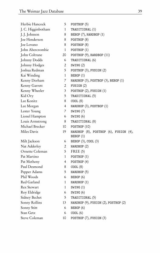
The Weimar Jazz Database 39
Herbie Hancock 5 POSTBOP (5)J. C. Higginbotham 1 TRADITIONAL (1)J. J. Johnson 8 BEBOP (7), HARDBOP (1)Joe Henderson 8 POSTBOP (8)Joe Lovano 8 POSTBOP (8)John Abercrombie 1 POSTBOP (1)John Coltrane 20 POSTBOP (9), HARDBOP (11)Johnny Dodds 6 TRADITIONAL (6)Johnny Hodges 2 SWING (2)Joshua Redman 5 POSTBOP (3), FUSION (2)Kai Winding 1 BEBOP (1)Kenny Dorham 7 HARDBOP (3), POSTBOP (3), BEBOP (1)Kenny Garrett 2 FUSION (2)Kenny Wheeler 3 POSTBOP (2), FUSION (1)Kid Ory 5 TRADITIONAL (5)Lee Konitz 8 COOL (8)Lee Morgan 4 HARDBOP (3), POSTBOP (1)Lester Young 7 SWING (7)Lionel Hampton 6 SWING (6)Louis Armstrong 8 TRADITIONAL (8)Michael Brecker 10 POSTBOP (10)Miles Davis 19 HARDBOP (8), POSTBOP (6), FUSION (4),
BEBOP (1)Milt Jackson 6 BEBOP (3), COOL (3)Nat Adderley 2 HARDBOP (2)Ornette Coleman 5 FREE (5)Pat Martino 1 POSTBOP (1)Pat Metheny 4 POSTBOP (4)Paul Desmond 8 COOL (8)Pepper Adams 5 HARDBOP (5)Phil Woods 6 BEBOP (6)Red Garland 1 HARDBOP (1)Rex Stewart 1 SWING (1)Roy Eldridge 6 SWING (6)Sidney Bechet 5 TRADITIONAL (5)Sonny Rollins 13 HARDBOP (9), FUSION (2), POSTBOP (2)Sonny Stitt 6 BEBOP (6)Stan Getz 6 COOL (6)Steve Coleman 10 POSTBOP (7), FUSION (3)

40 Martin Pfleiderer
Steve Lacy 6 HARDBOP (6)Steve Turre 3 POSTBOP (3)Von Freeman 1 FUSION (1)Warne Marsh 3 COOL (3)Wayne Shorter 10 POSTBOP (9), HARDBOP (1)Woody Shaw 8 POSTBOP (8)Wynton Marsalis 7 POSTBOP (7)Zoot Sims 6 COOL (6)

Computational melody analysis
Klaus Frieler
Introduction
This chapter provides an introduction into both the basic principles of com-putational melody analysis and their application and implementation inMeloSpySuite/GUI as developed and applied within the Jazzomat ResearchProject, especially within the case studies in the second part of this volume.The chapter addresses at a wide and diverse audience ranging from jazz re-searchers and musicologists seeking for an understanding of MeloSpyGUI,its possibilities and functionalities, to computer scientists who wishes tocomprehend or build on the concepts used within the software. Of course,both groups have different needs and different sets of previous knowledge.We tried to accommodate as many of these needs as possible and decidedon a dual strategy of using exact mathematical notations on the one handand verbal descriptions and concrete examples on the other. Mathematicalnotation might be hard to read or even off-putting for non-experts, but inthe spirit of reproducibility and transparency it is inevitable if one wishesto be as precise as possible for those who want to know or to recreate thedetails of an algorithm. Some mathematical basics as well as details regardingthe implementation of features and categories are included in ‘info boxes’along the main text. Additionally, there are short introductions to the FlexQquantization algorithm and into circular mathematics in the appendix. Wethink that those readers who are more interested in the applications andthe functionality of the software for jazz research as well as music researchin general can safely skip the formulas and stick to the verbal contexts andparticularly the examples. Nevertheless, a minimum openness to the mathmight be necessary for a more comprehensive picture.
This chapter focuses on three main topics: Firstly, the basic mathematicalconcepts for the computational representation of music used within the Wei-

42 Klaus Frieler
mar Jazz Database as well as the main annotation categories (segmentation,chords, meter and midlevel units) are explained. Secondly, both the generalconcepts of feature extraction and the most important musical features thatcan be extracted with our software are discussed. The features are groupedinto the main types in alphabetical order: accents, auxiliary, melodic contour,intervals, metadata, meter, pitch, rhythm, sequences of intervals pitch orrhythm, structure, and tone formation (including dynamics, articulation,and intonation). The last section is dedicated to the concepts of pattern searchand pattern mining which is a powerful tool within the MeloSpy software.
Music representation and annotation
Computational musicology aims to extract useful information from musicby using suitable (digital) representations of music. This is a very generaltask with many different approaches, depending on the concrete goals athand. It is very unlikely that any representational system will fulfill all pos-sible needs. In fact, quite a few representational systems have already beenproposed, implemented, and used. The best-known approach is commonWestern musical notation, which was originally developed for practical pur-poses. But since it features rather good mapping between scores and musicalobjects, musicologists and music theoreticians have used common Westernmusical notation for many centuries and are still using it today. In fact, itis still the most commonly used analytical representation. Many musicalrepresentation systems aim towards a digital version of common Westernmusical notation, e. g., MusicXML, MEI, MuseScore and Lilypond. But sincecommon Western musical notation is basically a prescriptive system fraughtwith a lot of historic conventions, idiosyncrasies, and implicit assumptions,it is not always well-suited for analytical tasks, e. g., for performance researchwhere information on micro-timing, loudness, and timbre is needed.
Moreover, since common Western musical notation is basically a graphical(two-dimensional) representation, encoding it to a digital format is not al-ways straight-forward and the results might not be well suited for analyticalpurposes due to of many purely graphical elements. Hence, computationalanalysis very often relies on more task-compatible encoding formats, e. g.,**kern, ABC, EsAC or MIDI, all of which have all their own advantagesand disadvantages. They are all based on certain (simplifying) assumptions,which reduce the expressiveness of the encoding, i. e., the amount of availableinformation.
In regard to expressiveness, audio files contain maximal information in thesense that they facilitate a re-creation of the sounding music with the aid

Computational melody analysis 43
of a suitable audio player. However, this maximal expressiveness comes at ahigh analytical cost, since a large amount of effort is necessary to extract theanalytically relevant information. This poses technological problems that cannot be deemed fully solved today, though impressive progress has been madein this regard in the field of music information retrieval (MIR) in the last twodecades. Music is ultimately a psychological phenomenon and the humancognitive system acts as a very powerful and specific filter system which, forexample, can easily extract the main melody from a complex polyphonictrack, a task that modern algorithms are still struggling with. Also, musicallyvery important phenomena such as beat induction and meter or tonalityperception are not easily defined and extracted from complex audio files,although these are often the focus of analytical endeavors.
In a more formal sense, a musical performance7 can be viewed (physically) asa sound-wave p(t ) over a bounded time interval T . This sound wave is thentransformed into a psychological representation p ′(t ) during listening. Wefurther assume that music differentiates into streams of (sonic, musical) eventseries. This assumption is strongly supported by research on auditory sceneanalysis (Bregman, 1990). Events in this context have a defined beginning(onset) and end (offset). The content of a musical event, however, cannot bedescribed easily in full generality, particularly not in psychological terms. Butvery often it can be agreed upon that musical events have certain qualities(qualias) such as pitch, loudness, and timbre as well as modulations of thesequalities.
Infobox 1: Mathematical basics: sets, maps, and sequences
The math used here deals mostly with ‘sets’, ‘maps’, and ‘sequences’. A set isbasically a collection of items, each counted only once and in no particularorder. Sets are notated using curly brackets which embrace either a list ofelements or some sort of condition that defines the elements in the set. Forexample, A= 1, . . . ,N is the set of the first N natural numbers. Standard setsoften used in the context of computational musicology are the natural numbers(symbol N), the integer numbers (symbol Z), and the real numbers (symbolR). To indicate that x is contained in a set A, one writes x ∈ A. For example,17 ∈N. The empty set with no elements is notated ;. The numbers of elementsin a set A is written as |A|. Sets can have infinitely or finitely many elements.Sets can also have subsets, notated A ⊂ B . Sets of consecutive numbers are
7We do not wish to go into the complicated discussion of what music actually is here, butsimply take this as an externally given label. However, in certain audio engineering applica-tions, it is an important to classify chunks of audio files into music or non-music, e. g., speech,environmental noise, or bird song.

44 Klaus Frieler
very important in the context of computational musicology and are writtenas [N : M ] = N ,N + 1, . . . , M, which means all integers between N and Mincluding M . It holds [N : M ]⊂N. Intervals of real numbers are written with acomma instead of a colon, e. g., [x, y] is the interval of all real numbers betweenand including x and y. Sets have intersections A∩B , i. e., the set of all elementsboth in A and B , and unions A∪ B , i. e., the set of elements either in A or B .Large symbols are used to indicate intersections and unions of more than oneset, e. g.,
⋃
1≤i≤N Ai is a shorthand notation for A1 ∪A2 ∪ · · · ∪AN . Anotherimportant construction is the so-called Cartesian product. For two sets A and Bthe Cartesian product A×B is the set of pairs (x, y)where x ∈A and y ∈ B . Thisalso works for more than two sets, and the elements are then called N-tuplesfor a Cartesian product of N sets. The order is important, i. e., A×B 6= B ×A.Maps are collections of arrows between two sets, starting in a domain set, say A,and ending in a image set (or co-domain), say B . A map from A to B is writtenas M : A→ B . If one wants to express the mapping of a concrete element in thedomain to an element in the image of M , one writes x 7→ y = M (x). Not allelements in B have to be the endpoint of an arrow. Likewise, not all elementsin A need to be a starting point, but in most cases we will assume this to be thecase. We also assume that at most one arrow points from each element in thedomain to an element in the image set. Maps can also be defined between maps,which will be encountered quite often in computational musicology, e. g., inthe case of transformations or vector features. This comes from the fact thatsequences play an important role.A sequence is simply a collection of elements with an order; thus, one cansay such things as “element x appears earlier than element y in the sequence”.Since the integer numbers have a natural order of this kind, they can be usedto define sequences as maps from integer intervals onto a certain image set X .For example, x : [1 : N ]→X , with i 7→ x(i) ∈X . Very often, index notationis used for this, i. e., i 7→ xi . Another compact notation for this is with simpleparentheses (xi )1≤i≤N , or, even lazier, just xi . An explicit listing of elements inparentheses means that it is a sequence or a tuple and not just a set.
In some cases, e. g., for percussive events, a simple (task-relative) categoriza-tion might be sufficient, e. g., naming the percussive instrument that hasproduced the event. In other cases, a justifiable simplification is to use a con-stant single pitch as a sole descriptor, whereby pitch is represented with asymbol (e. g., a note name) or a number as a proxy derived from the funda-mental frequency ( f0) of the event. These events are called tone events. Chordscan then be represented as collections of pitches (and further abstracted intochord symbols).
In the context of the Jazzomat Research Project, we are dealing exclusivelywith monophonic solos and therefore use exactly this simplified represen-

Computational melody analysis 45
tation as a core, complemented by various annotations. Formally, thus, amelody is a discrete times series
ti 7→ ei = (ti , di , pi ),
where an event ei is described by a triple (ti , di , pi ) of numbers which repre-sent
• onset ti (seconds),
• duration di (seconds),
• and a (constant) pitch value pi (MIDI number),
of a tone event.
Pitch values are represented by indices in the 12-tone equal tempered system,using the well-known and common MIDI indexing scheme (Selfridge-Field,1997), which represents an associated f0 value via the formula8
p = 12
log2f0
440 Hz
+ 69,
where the square brackets mean taking only the integer part. The note A4=440 Hz is mapped to MIDI index 69 and every octave equals 12 semi-tonesteps, e. g.,
A3 (220 Hz) 7→ 12 log212+ 69=−12+ 69= 57,
orA5 (880 Hz) 7→ 12 log2 2+ 69= 12+ 69= 81.
The number of events in a melody is called its length, whereas the durationof a melody is defined as the difference between the onset of its first elementand the offset of its last event. For the following, we will use the conventionthat the first element in an event series is indexed by 0 (zero-indexing). Hence,a melody of length N is indexed with 0 . . .N − 1. For intervals of integernumbers we will adopt the notation [N : M ] for the set of integers betweenand including N and M (with M ≥ N ). Formally, a melody of length N isthen a map e : [0 : N − 1]→R×R+× [0 : 127].
8The actual transcription process for the Weimar Jazz Database was performed by humantranscribers who assigned the most fitting pitch to a tone event. See Chapter Score-informedaudio analysis of jazz improvisation for measuring the exact intonation of the played tones.

46 Klaus Frieler
A melody is defined as monophonic, which means that its onsets should bestrictly ordered (ti < ti+1, for all i ). In a strictly monophonic melody, eventsdo not overlap, i. e., the offset ti + di of an event should be smaller thanor at most equal to the onset of the following event, ti + di ≤ ti+1 for all i .The inter-onset intervals (IOI) are then defined as the differences of onsetsbetween consecutive events, IOIi = ti+1− ti . Note that there are one fewerIOI than there are events. Semitone intervals are defined as differences ofpitches between consecutive events,∆pi = pi+1− pi . An elementary set ofoperations that can be applied to melodies or series is a projection, which is aformal term for ‘forgetting information’. A projection means to only use asubset of the information, e. g., onsets, durations, or pitches or combinationsthereof. For example, the sequence (ti ) is the list of onsets, the sequence (pi )is the pitch sequence derived from a melody, and so on. Using only partof the information in a melody (or annotated melody, see below) is a verycommon technique for constructing features and defining patterns.
Figure 1: Beginning of Chet Baker’s solo on “Let’s Get Lost”, also known as the “TheLick”.
Example. The core representation and some derived values of the melodydepicted in Figure 1 (in common Western musical notation) can be foundin Table 1. In output files of the MeloSpyGUI the value NA (not available)is mostly used for this. Note that the difference values IOI and interval areattached to the first interval here, which is the convention used in the Jazzo-mat Research Project; other authors prefer to attach it to the second value.However, attaching difference values to the first element often simplifiessubsequent computations.
Annotations
Obviously, this core representation of a melody is rather bare-bone and ofonly limited analytical value (although it already allows for the derivation ofpitch and interval features as well as Markov models and very basic rhythmanalysis). Thus, it is desirable to ‘thicken’ this description of tone eventswith a flexible annotation system, which allows the ‘tagging’ of additionalinformation to an event or a series of events. Most annotations are generatedexternally, mostly by humans, and are not directly derivable from the basic

Computational melody analysis 47
Table 1: Core representation and some derived values of the beginning of Chet Baker’ssolo on “Let’s Get Lost”.
Core representation Derived values
Note Onset (s) Duration (s) Pitch Offset (s) IOI (s) Interval
1 2.667 0.195 71 2.862 0.395 02 3.062 0.087 71 3.150 0.166 -23 3.228 0.194 69 3.422 0.221 24 3.448 0.190 71 3.638 0.192 15 3.640 0.190 72 3.830 0.200 26 3.840 0.161 74 4.001 0.200 -37 4.040 0.280 71 4.310 0.360 -48 4.400 0.155 67 4.555 0.244 29 4.644 0.673 69 5.317 n. d. n. d.
Note. n. d. = not defined.
representation. Most annotations are generated only once and then storedalong with the basic presentations. Hence, the term annotation expresses amore practical distinction to transformations and features, as described belowin p. 60.
One has to differentiate two types of annotations: local and contextual. Lo-cal annotations pertain to the event itself and are directly derived from it.Important examples are acoustical features such as f0 modulations (vibrato,slides etc.), intensities/loudness or timbre (cf. Chapter Score-informed audioanalysis of jazz improvisation). Contextual annotations are only derivablewith respect to a certain context of an event, e. g., segmentations (cf. Infobox2). However, contextual annotation can always be represented (and stored)as local annotations to certain events, e. g., a phrase segmentation can beexpressed by annotating phrase IDs. The contextuality must then be reflectedby certain consistency conditions, e. g., the phrase IDs of two adjacent eventsmust be equal or the second must be greater than that of the first.
Formally, we define an annotated melody as the map
ti 7→ (ei ,ai ),
where ei is the core representation (ti , di , pi ) and the annotations
ai = (ai1,ai2, . . . ,ai M )
are M -dimensional tuples of values (i. e., vectors of M values for each event).
48 Klaus Frieler
The only condition imposed on an annotation is applicability to each eventin a series (which can always be fulfilled trivially by allowing the empty setor a similar special symbol as a valid annotation value). We will encounterseveral important annotations (e. g., metrical and chord annotations) in thefollowing sections.
Segmentations
Segmentations play an important role in computational musicology. Theyoccur naturally, e. g., in the form of melodic phrases, during melody per-ception (Lerdahl & Jackendoff, 1983). Segmentation simply refers to sets ofsubsequences or segments. A subsequence is any consecutive patch of a series,i. e., without ‘holes’. Formally, a subsequence of a melody e : [0 : N −1]→ eiis a restriction on [k : l ] with 0 ≤ k ≤ l ≤ N − 1. We will notate such asubsequence as ek:l .
Two main kinds of segmentations can be differentiated: overlapping and non-overlapping. Overlapping segmentations contain segments that can sharecommon events, whereas in non-overlapping segmentations segments aredisjunctive. Exhaustive segmentations are those for which every event is con-tained in at least one segment. Pattern partitions (s. p. 82) are an importantexample of non-exhaustive overlapping segmentations, whereas phrase andchord annotations are an example for exhaustive non-overlapping segmenta-tions. Very often, segmentations are themselves equipped with some kind ofannotation, e. g., an ID or a value of arbitrary type, cf. Infobox 2 for exam-ples. In the following, we will briefly discuss three important segmentationtypes—form parts, chord and midlevel annotation—which are specific to thejazz solos in the Weimar Jazz Database.
Infobox 2: Segmentations in the Weimar Jazz Database
Several important segmentations are included in the Weimar Jazz Database andaccessible via different mechanisms in the MeloSpyGUI. On the database level,the following (exhaustive, non-overlapping) segmentations are available.
• Phrase IDs These are integer IDs, starting with phrase 1, for each phraseannotated by the transcriber.
• Chord annotations. These contain chord symbols for each event underthe scope of this chord, which were manually annotated to the beat track.See Infobox 3 and Chapter The Weimar Jazz Database.
• Form parts. Annotated according to the lead sheet. Each event is also
Computational melody analysis 49
part of a form part which is represented by specific form part symbols(e. g., A1, B2).
• Chorus IDs. Each solo consists of one or more choruses, i. e., cycles ofthe underlying form as embodied in the chord sequences. Chorus IDs areintegers, starting from chorus 1. However, sometimes there are pick-upbars, i. e., a solo starting slightly before the beginning of a new formcycle. These pick-ups are notated as chorus ID -1.
• Midlevel Units (MLU)→ p. 54.
Segmentations are stored in the Weimar Jazz Database in the SECTIONS tableusing the IDs of the first and last element index of the segmentation in the anno-tated melody plus the annotated value/ID. All these segmentations can be usedin the MeloSpyGUI during feature extraction to chop a melody into segmentsfor which features are calculated. There are also auxiliary features which addthe values/IDs for direct event-wise annotations. Additionally, segmentationswith bar chunks can be chosen, which will segment the melodies/solos intoconsecutive patches of bars of arbitrary length with user-definable overlap (i. e.,these are overlapping, exhaustive segmentations if the overlap is not empty).
Chord symbols
Chords play a major role in jazz improvisation, thus a comprehensive rep-resentation of chords is vital for the computational analysis of jazz solos.Consequently, the beat tracks in the Sonic Visualiser project files of the solotranscriptions have been annotated with chord symbols taken from leadsheets. Chord annotations are included in the Weimar Jazz Database and are,for instance, used for chord-related pitch representations (s. p. 63).
A chord is basically a pitch class set with a certain structure, in which the rootis the most important tone. Chords are represented by chord labels, whichhold all relevant information and follow a certain syntax. The MeloSpyGUIchord syntax is designed to match the chord symbols that are in practical (jazz)use as closely as possible. Internally, a CHORD object consists of a root note,a triad type (major, minor, diminished, augmented, half-diminished/7[5)and an optional bass note (for slash chords and inversions). Sevenths (major,minor, or diminished), ninths (natural, flat, or sharp), elevenths (natural orsharp), and thirteenths (natural or flat) are optional.
Instead of using existing chord syntax (e. g., Harte, Christopher, Sandler,Samer, & Gómez, 2005), we decided to devise our own, closer to traditionalchord symbols, in order to facilitate annotation and readability. However,

50 Klaus Frieler
very often users will not have to deal with the low-level chord annotations,since during exporting, internal chord symbols are translated back to standardnotation. For sake of completeness, and for those users who would like toproduce their own Sonic Visualiser project files in our format, the syntax canbe found in Infobox 3.
Infobox 3: Chord syntax
Chords are expressed using the following grammar. The grammar should beread as follows: Each line contains a definition of an expression, indicated bythe ::= sign, where small letter names represent other expressions and quotedstrings are the terminal symbols. For example, a chord can either be the ‘nochord’ expression, which is the string NC, or a normal chord, defined on thethird line, or a special chord, defined on the fourth line. Vertical bars denotealternatives and square brackets denote optional elements. For example, anaccidental can be either a sharp (]) or a flat ([) and a ‘generic note name’ is noteletter (‘A’ to ‘G’) optionally followed by an accidental.Note that some conveniences and optional expressions are included to facilitateannotation. The main difference to standard notation (e. g., in the Realbook)is that accidentals of chord tensions are placed after the number. For instance,a C7]9]11[13 chord is translated to C79]11]13b. The usual implications of lowertension in the presence of a higher tension also apply. Hence, a Cm11 notatedas C-11 or Cm11 automatically includes the sevenths and the ninth as well andis therefore equivalent to C-7/9/11. Currently, no mechanism is included for‘adding’ single tension without implications. For example, a Cadd9 with addedninth but without the seventh is not expressible in our chord syntax.
chord ::= no_chord | normal_chord | special_chordno_chord ::= "NC"normal_chord ::= generic_note_name triad_type
[seventh] [ninth] [eleventh] [thirteenth][slash_expr]
special_chord ::= generic_note_name exception [slash_expr]generic_note_name ::= note_letter [accidental]note_letter ::= "A"-"G"accidental ::= sharp | flatsharp ::= "#"flat ::= "b"triad_type ::= major | minor | augmented |
diminished | suspendedmajor ::= "maj" | ""minor ::= "min" | "m" | "-"augmented ::= "aug" | "+"diminished ::= "dim" | "o"

Computational melody analysis 51
suspended ::= "sus"seventh ::= ["j"]"7"ninth ::= "9" accidentaleleventh ::= "11" [sharp]thirteenth ::= "13" [flat]slash_expr ::= "/" generic_note_nameexception ::= "7b5" | "alt" | "7#9" |
"m7b5" | "7sus4" | "maj7"
Metrical annotation
Metrical frameworks are very important for the perception and productionof music around the world. The perception and induction of a beat is aprecondition for the occurrence of the phenomenon of meter. For our repre-sentation of the musical surface, we adopted a very general framework whichworks with minimal assumptions, e. g., without presupposing a deeply nestedmetrical hierarchy.
The basic conception puts the beat level in the center, with beats not beingassumed to be isochronous, or even regular, but are essentially just a series oftime points. Internally, a beat is stored as an onset with a duration, which isthe interval between consecutive beats, i. e., the inter-beat interval (IBI).
In our metrical framework, there are only three hierarchical levels: Beatsare grouped into units (‘measures’) of certain length (called ‘period’) on onehand, and divided into sub-beat levels (‘tatums’) on the other; no regularityassumptions are made for either. A sequence of measures with constantlyvarying periods can be represented as well as beat-wise changing subdivisions,which are not required to be of equal length although this is common. Ametrical framework has to be differentiated from a concrete realization ofthis framework. For transcriptions, the task is often to infer an underlyingmetrical framework to a certain realization of a musical rhythm, which mightnot be unequivocal. For the transcriptions in the Weimar Jazz Database, thecore part is implemented via human annotations, i. e., based on manualbeat tracks with annotated time signatures. To accelerate and facilitate thetranscription process, the annotation of musical tones to metrical positionis done algorithmically based on the beat track and the tone onsets. Thisalgorithm, called ‘FlexQ’, was specifically devised in the context of the Jazzo-mat Research Project and is described in more detail in Appendix The FlexQ
52 Klaus Frieler
algorithm (see also Frieler and Pfleiderer (2017) for a discussion of generalissues with respect to metrical annotations).
First, we will introduce some notations and concepts. A beat track is a se-quence of time points ti , with inter-beat intervals∆ti := ti+1− ti . The inverse
1∆ti
of the inter-beat interval is the (instantaneous) tempo of the beat track.
A metrical annotation of the beat track is a mapping of beat times to pairs ofinteger values ti → (p j (i ), bk j
(i )) subject to the following conditions: p j ≥ 1and 1 ≤ k j ≤ p j for all j . The numbers j are the bar numbers, the p j arethe periods (number of beats in a bar j ) and the bk j
are the beat indices inthe j -th bar, running from 1 to p j . A shorthand notation for the metricalannotation is mi = ( j (i), p j (i), bk j
(i)).
Example. Assume an (isochronous) series of six beats (cf. Figure 2). A 2-periodmetrical annotation, using the shorthand notation, would then be given by
(1,2,1), (1,2,2), (2,2,1), (2,2,2), (3,2,1), (3,2,2),
and a 3-period one by
(1,3,1), (1,3,2), (1,3,3), (2,3,1), (2,3,2), (2,3,3).
A mixed 4-period/2-period annotation is also feasible:
(1,4,1), (1,4,2), (1,4,3), (1,4,4), (2,2,1), (2,2,2).
Since the numbers are only a function of the beat indices i , but not of theactual beat times ti , this representation is purely abstract. Consequently,given such a metric representation, any series of beat onsets can be viewed asa realization of such a metric framework.
To establish a connection to an actual perceived meter, the beat times shouldfulfill certain criteria, e. g., approximate isochrony. Note that, in contrastto common Western musical notation’s time signatures, only the numberof beats per group (periods) are provided. No distinction is made between24 or 2
2, or 68, all of which have two beats grouped into a bar. The difference
between 24 and 6
8 is that in the former one beats are more likely to be subdividedbinarily, whereas in the latter the prevalent subdivision is ternary. Note, thatbinary or ternary subdivisions are not a fixed rule, but only prevalences,e. g., triplets occur less often in 2
4 and duplets (dotted eighths notes) in 68. The
system proposed here leaves this mostly to the user and simply provides asystem for annotating arbitrary subdivisions for each beat. This brings us tothe general definition of a metrical annotation.

Computational melody analysis 53
(1, 2, 1) (1, 2, 2) (2, 2, 1) (2, 2, 2) (3, 2, 1) (3, 2, 2)
(1, 3, 1) (1, 3, 2) (1, 3, 3) (2, 3, 1) (2, 3, 2) (2, 3, 3)
(1, 4, 1) (1, 4, 2) (1, 4, 3) (1, 4, 4) (2, 2, 1) (2, 2, 2)4/2−period
4−period
2−period
Figure 2: Three different sample metrical annotations of a six beat sequence. Solidlines: first beat of a bar; dashed lines: all other beats. Annotations are given in theformat (bar number, period, beat index).
Consider an arbitrary rhythm, i. e., a series of time-points ti . A metricalannotation for this rhythm is then a map onto tuples of five integers
( j , p j , bk j, dk j
, sm),
where ( j , p j , bk j) is a beat annotation as defined above, dk j
∈N is the divisionof the beat bk j
, and 1 ≤ sm ≤ dk jis the tatum position below the beat bk j
,which runs between 1 and the division of the beat.
Example. Consider the rhythm of the ‘The Lick’ in Figure 1. The metricalannotation consists of two bars (mm. 1 and 2), both of period 4. The first twonotes are each placed on the second tatums of beat 1 and 2. The followingfour eighth notes are on tatum 1 or 2 of the binary subdivided beats 3 and4. The next note is on tatum 1 of the undivided first beat of the second bar,while the last two notes are on tatum positions 2 and 4 of beat 2 with a4-subdivision (sixteenth notes). Rests are not considered here. The resultingmetrical annotations can be found in Table 2 and Figure 3.

54 Klaus Frieler
Infobox 4: Metrical position notation
For output purposes, the MeloSpyGUI uses a special dot-notation formetrical positions. The format is
period.division.bar_number.beat_number.tatum_position
period is the number of beats in a bar. If beat_proportions are set(for non-isochronous beats), beat_proportions will be used instead ofperiod in an ‘additive’ notation, e. g., (3+2+2). division is the numberof tatums in the current beat. The other fields are bar number, beatnumber, and tatum position.
Midlevel annotation
Midlevel analysis (MLA) can be regarded as a short and compact system tosegment the musical surfaces into sections of sufficiently distinct character.These units are called midlevel units (MLU). It was developed in an attemptto identify underlying playing ideas of jazz improvisations. The approachwas first developed for piano solos (Frieler & Lothwesen, 2012; Schütz, 2015)and then adapted for monophonic solos (Frieler et al., 2016a).
MLA is based on the hypothesis that jazz players are more likely to makedecisions on a middle level (with regard to playing details), comprising timesspans of a few seconds, which are then actualized using preconceived orspontaneous material from motor memory. This guiding principle led to theidentification of several distinct types of ideas by analyzing a large sample ofsolos. First, solos were segmented into parts of discernibly different character,which were tentatively named. In a second step, these types were condensedand re-ordered by simultaneously establishing a comprehensive system of sub-and sub-subtypes. In principle, this typology of playing ideas is not closed,but can be considered saturated for the Weimar Jazz Database, in the sensethat it is possible to typify all playing ideas into one of the devised types.However, with new data or data of a different kind, it might be desirable toadd new types if enough ideas are encountered that cannot be reasonablywell fitted into one of the existing categories. For example, due to instrumentspecifics, playing ideas for piano solos and monophonic solos are not identical,although a large overlap exists. There is evidence that piano players, when

Computational melody analysis 55
Table 2: Metrical annotation of the rhythm of ‘The Lick’.
Note TAS Metrical annotation Dot notation( j , p j , bk j
, dk j, sm) (p j , dk j
, j , bk j, sm)
1 1+ (1, 4, 1, 2, 2) 4.2.1.1.22 2+ (1, 4, 2, 2, 2) 4.2.1.2.23 3 (1, 4, 3, 2, 1) 4.2.1.3.14 3+ (1, 4, 3, 2, 2) 4.2.1.3.25 4 (1, 4, 4, 2, 1) 4.2.1.4.16 4+ (1, 4, 4, 2, 2) 4.2.1.4.27 1 (2, 4, 1, 1, 1) 4.1.2.1.18 2e (2, 4, 2, 4, 2) 4.4.2.2.29 2a (2, 4, 2, 4, 4) 4.4.2.2.4
Note. Note= note number in the example from Figure 1 and Table 1;TAS = traditional American system for counting metrical positions(second sixteenth= e, eighth=+, fourth sixteenth= a); metrical an-notation as defined in the text; dot notation =metrical dot notationused in the MeloSpyGUI, see Infobox 4.
Figure 3: Metrical annotation for ‘The Lick’. Thick vertical lines correspond to theonsets, thin lines to annotated beats. Labels are given in metrical dot notation for theonsets and in the format (bar number, beat index) for the beats.

56 Klaus Frieler
confronted with the system, find the concept at least partly adequate forinternal improvisation processes, though possibly not with regard to alldetails of the typology (Schütz, 2015). However, the exact connection toactual playing ideas is still an open research question. Besides identifyingdistinct MLUs, the system also incorporates an easy way to encode musicalrelationships and similarities between MLUs, e. g., variations, which permitinteresting insights into the process of improvisation and an examination ofdramaturgy and form.
1. line:9 A line is a series of tones for the most part proceeding in small,step-sized intervals with high rhythmical uniformity and a salient tra-jectory in pitch space. Depending on the trajectory, there are severalsub- and sub-subcategories. The main subcategories are simple (default),tick, interwoven, and wavy lines. The main shapes are ’horizontal’,‘ascending’, ‘descending’, ‘concave’, and ‘convex’. Tick lines are lines ofexclusively convex and concave shapes but with asymmetric arms, i. e.,a longer or shorter descent or ascent combined with an accordinglylonger or shorter ascent or descent. Simple lines show a straight direc-tion, i. e., without too many twist and turns, which are characteristic ofwavy lines. Wavy lines tend to be rather long and may have an overalldirection besides ‘wiggling around’. Interwoven lines consist of twoindependent horizontal ascending or descending lines that are playedin tone-wise alternation.
2. licks: In the context of MLA, a lick is a rather short and concise melodicfigure that often includes rhythmical and intervallic salience. Licks havea clear gestalt-like quality, which distinguishes them from fragments.They comprise mostly short tones and sometimes large intervals andchromaticism, which distinguishes them from melodies. Shortness,rhythmic diversity, or both qualities together separate licks from lines.We have two proper subtypes in this category: lick_bebop and lick_blues.All other licks are grouped into a residual subclass lick. Blues licks aredefined by tonal features such as blue notes as well as typical construc-tions. Historically, the blues played (and still plays) a special role injazz improvisation (Schuller, 1958), so it seemed worth defining a spe-cial subcategory. Bebop licks on the other hand use certain techniqueswhich are typical for bebop lines, such as approach notes and chromaticpassing tones.
9The following description of the nine main MLU types is a slightly edited version takenfrom Frieler et al. (2016a).

Computational melody analysis 57
3. melody: A melodic figure that is not derived from the theme of thesong and embodies some kind of song-like, lyrical, cantabile character.A rule of thumb may be: If an MLU sounds more like scatting (if sung),it should be termed a lick or a line; if it sounds more like a Broadwaytune, a pop song or a folk tune, it should be labeled as melody.
4. rhythm: This category describes units in which the rhythmical expres-sion is the single most prominent feature. There are four subtypes thatdiffer according to the number of pitches (single or multiple) and basicrhythm quality (regular or irregular). The most important subtypesare single tone repetitions, predominantly regular and isochronous,and oscillations with multiple tone repetitions, predominantly regular.
5. theme: Denotes material taken directly from the theme of the tune,possibly with variations. The characteristics of a theme MLU are oftensimilar to those of melody, but because of its relationship to the tune,it is a distinct playing idea.
6. quote: These are direct quotes from another piece of music (jazz tune,classical tune etc.), which might resemble a melody or a theme. Playinga pattern taken from another jazz musician as part of a longer line or alick does not count as a quote if it is not clearly recognizable as such.
7. fragment: A small set of tones which neither form a clear contour-based succession or motivic/thematic figure nor are very expressive.Fragments are most often single tones or very short segments whichcan even sound like ‘mistakes’.
8. expressive: These are figures or single tones with a sound- or gesture-like character in which aspects of expressivity are clearly focused, e. g.,scream-like sounds.
9. void: This category refers to moments of ‘actively playing nothing’.Generally, jazz soloists add short breaks between phrases, e. g., justfor breathing, which do not belong to this category. The length ofthe break in the flow of a solo should clearly exceed these usual gapsbetween phrases.
All solos in the Weimar Jazz Database were manually annotated with MLUsby three annotators. Special care has been taken to ensure that the MLUtypes are consistently annotated. One annotator double-checked all otherannotations. As this is basically a qualitative system with categories thatcannot be defined unequivocally and which have continuous and overlapping

58 Klaus Frieler
boundaries, there is some leeway for the annotators. However, when compar-ing annotations of three to four different coders using a small subset of solos,high agreement (Fleiss’s κ = .81) for assignment of MLU boundaries wasfound, whereas the agreement for MLU types was lower (Fleiss’s κ= .60),but still sufficiently good. The main disagreement was between line and lickas well as between melody and lick. For specific MLUs, disagreements be-tween different coders might come about due to the fact that several equallyadequate solutions exist, but each MLU has to be assigned to exactly one type.Even when annotations might disagree, they can often still be considered as‘correct’ (or ‘not wrong’). Hence it can be safely assumed that for statisticalanalyses the disagreements level each other out and that the resulting statis-tics are sufficiently valid. The most common MLU type is, not surprisingly,lick with about 45 % followed by lines 30 %. However, since licks are muchshorter than lines, they only account for about 37 % of the duration of allsolos, whereas lines account for about 40 %. For more details about MLUstatistics and distributions in the Weimar Jazz Database, we refer to Frieleret al. (2016a).
Infobox 5: MLU syntax
For the MLA annotation in Sonic Visualiser, a specific short mnemonic codewas devised (see Online Supplementary Material S2 of Frieler et al., 2016a).The basic rule is that a musical phrase starts an MLU, but that more thanone MLU can be contained in one musical phrase, which is called ‘glueing’.Each MLU contains information about its type (full type with all possible sub-subtypes), whether the MLU is glued on, possible reference or relationship to aforegoing MLU (called ‘back reference’), some additional information aboutthis relationship, and finally comments of further specification.The basic syntax is:
[~][#[N][*+-=]]cat-label[:specifier]
where square brackets denote optional elements. The first element, the tilde ~,if present, indicates a glued MLU. The hash #, followed by an optional integernumber N indicates a back reference to the MLU N MLUs before. If N is missing,a value of one is assumed, i. e., a relationship to the immediately precedingMLU. Equivalently, this can also be expressed by sequences of N hashes. Thefollowing symbols *+-= indicate the type of relationship, if clearly identifiable.The asterisk * indicates an unspecified variant and can be omitted. The plusand minus signs denote transpositions up + or down - in pitch space, wherebythe transposition does not need to be exact (hence an asterisk is implied). Forexact (possibly transposed) repetitions, the equal sign = can be used.The cat-label has to be one of the following:

Computational melody analysis 59
• Licks: lick (unspecified), lick_bebop (bebop lick), lick_blues (blues lick).
• Simple lines: line_a (ascending), line_d (descending), line_cv (concave),line_cx (convex).
• Tick lines (a= ascending, d= descending, s= short, l= long): line_t_asdl,line_t_alds, line_t_dsal, line_t_dlas.
• Interwoven lines (a = ascending, h = horizontal, d = descending, topline first) : line_ah, line_ha, line_ad, line_hd, line_aa, line_ad, line_da,line_dd.
• Wavy lines line_w[_x], where x can be any specifier from simple andtick lines or missing, which is short for line_w_h, a wavy line that startsand ends roughly at the same pitch.
• Rhythms (s = single pitch, m =multiple pitches, r = regular rhythm,i = irregular rhythm): rhythm_sr, rhythm_si, rhythm_mr, rhythm_mi.
• Others: melody, void, expressive, quote, theme.
The specifier part is optional and can be any string, e. g., the name of the musicalwork a quote was taken from or the location in the theme of a theme reference.Examples. ~#2+melody is a glued melody that is an upwardly transposedvariation of the MLU (not necessarily also a melody) two units before; theme:t1is a reference to measure 1 of the theme of the tune; lick, #lick, #lick is a chainaa’a” of successively varied licks. If more than one back reference is possible, asprobably here for the last one, the shortest back reference should be taken.
Feature extraction
Feature extraction is one of the central tasks in computational musicology anda prerequisite to many analytical investigations. In a general sense, featurescan be conceived as characteristics, traits, or properties that describe specificentities, e. g., musical objects. They range from very simple features, whichrequire only a trivial measurement or are part of the definition of an object,to very complex ones (‘deep stucture’), which require elaborate measurementprocedures or cognitive models. Moreover, features can be ascribed to thewhole entity of interest or only to parts of it. They can be single values (e. g.,the number of notes in a melody) or vectors of symbols (e. g., the title of apiece.)
Features often serve as dependent variables in models to predict target vari-ables, e. g., music perceptions or style classification. For example, certainmusical properties, such as tempo, articulation, or tonality, are known to con-

60 Klaus Frieler
tribute to the emotional expression or impact a piece of music can have. Forclassification, objects are grouped into classes, categories, or types accordingto certain properties, i. e., feature values, using suitable similarity measures.Features are essentially human constructions and seldom merit ontologicalstatus. They coordinate the relationship between the objects and operationalmodels for the prediction and description of these objects, but are principallyarbitrary and contingent on the purpose of the scientific model. In analogy tocoordinate systems that describe physical objects in space, one can also speakof ‘feature spaces’ for the description of an object. Like coordinate systemsin the physical world, certain features are more apt or easier to handle thanothers, depending on the tasks and objects at hand. Finding the most suitablefeatures for a problem is often a central task, called ‘feature selection’.
There are always possibilities for constructing new features from old onesusing algorithmic or mathematical operations. This is basically the approachwe followed in designing our feature extraction software (melfeatures). Ithas a flexible module (‘feature machine’) at its core that allows the definitionof a large class of features based on certain predefined properties of the musicalobject (i. e., its basic representation) and a set of mathematical and statisticaloperations.
General concepts
It is useful to first define some general properties of features. Let O = oibe a set of objects and F = F1 × F2 × · · · × FN an arbitrary feature space.The number N is called the dimension of the feature space, where we assumethat the components Fi are mostly elementary (one-dimensional). In mostcases, the components are either real or integer numbers (Fi =R,N) or a setof labels, i. e., an arbitrary set with no further internal structure.
A feature is then a map from the objects into the feature space. The primaryor defining features are those which are used to define the objects. Please notethat the abstract representation of objects here is not identical to the objectsthemselves, i. e., the objects of interest here are the digital representations ofmusical objects as defined in section p. 41. Hence, in our representation, theprimary feature of a melody is the representation itself, i. e., tuples of onsets,durations, and pitches etc. In this approach, each object has to have its ownfeature space, since the dimension of the basic representation is dependenton the length of the melody. The representation space for a melody of lengthN is then effectively 3N dimensional with components Fi = R × R+ ×[0 : 127]. Feature maps where the feature spaces vary with the object arecalled sequential features or, alternatively and probably less confusingly,

Computational melody analysis 61
transformations. Such transformations can themselves, of course, becomethe starting point of another feature map and in this way transformationchains can be built. This is also the basic logic behind the ‘feature machine’of the melfeature module of MeloSpyGUI software, where transformationchains are defined with the aid of a simple syntax.
An important special case of feature maps are global features, which mapan object to one and the same feature space. If the feature space is one-dimensional, these are called scalar features, even if the feature space is notnumerical. Metadata are an important case of global and scalar feature. Forexample, the solos in the Weimar Jazz Database have an annotated rhythmfeel which is represented by the set of labels
R = SWING,LATIN,FUNK,TWOBEAT,MIX.
Then, the ‘rhythm feel feature’ is a map from the solos S →R onto theset of rhythm feel labels. Similar constructions hold for all metadata, eventhough the feature space is not always a fixed set of labels, but often strings(character sequences), e. g., the title of a piece.
Phrase IDs are an example of a non-primary sequential feature. Since eachsolo has a different number of phrases, a global finite-dimensional featurespace is not sufficient to represent all possibilities. We can formally solve thiswith the aid of sequence spaces, e. g., spaces of sequences of arbitrary lengthinto a fixed target space. Let T be such a target space (in the case of phraseIDs, these are the integers, T =N). A sequence of length N over T , denotedSN (T ), is a map [0 : N −1]→ T . The space of all sequences over T is definedas the union of all sequences of positive length:
S (T ) =∞⋃
N=1
SN (T ) = S1(T ),S2(T ), . . ..
Note that sequences of length 1 are identical to the target space itself,S1(T ) =T . A sequential feature (also sometimes, a bit misleadingly, called vectorfeature) is a feature map with feature space S (T ). The list of phrase IDs of asolo is then a sequence of integers from 1 to M , where M is the number ofphrases in a solo. Of course, such a list of integers is not very informative, soit can be combined, for example, with the indices of start and end tones tounequivocally identify phrases within a certain solo.
Our basic representation of melodies can then be viewed as a sequentialfeature with feature space S (R×R+× [0 : 127]). In the case of sequentialmusical objects, a sequential feature is called point-wise or local if the lengthof the sequence space is (a simple function of) the length of the melody. In

62 Klaus Frieler
other words, a transformation that results in a sequence of the same length asthe original melody is ‘local’ in this sense.
Finally, a matrix feature is a feature map into the space of matrices (mostlyover R), where the dimension of the matrices can be dependent on the ob-ject itself. A prominent example, available in the MeloSpyGUI, is the self-similarity matrix of phrases (see p. 63).
An important class of—mostly global—features are statistical features. Theseare constructed by using descriptive statistics (e. g., mean, median, standarddeviation etc.) of a sample distribution which in this case are the elements of atransformation chain. For example, the mean pitch of a melody is constructedby the projection on the pitch component and subsequent averaging all(MIDI) pitches pi of a melody of length N , i. e.,
p =1N
N−1∑
i=0
pi .
A more complicated example is the relative frequencies of a chordal pitchclass. Chordal pitch classes are defined for a pitch p and an annotated chordCp with root pitch class r (Cp ) ∈ [0 : 11]. The chordal pitch class of p is thendefined as the interval of p to the root modulo 12. The modulo 12 operationreturns the remainder after an integer division by 12, e. g., 23 mod 12= 11.This operation effectively disregards the octave. The full formula is then:
γ (p,Cp ) = (p − r (Cp )) mod 12.
Applying this transformation to a melody of length N results in a sequence ofchord pitch classes γi = γ (pi ,Cpi
), also of length N , which can then be treatedas a random sample over the numbers from 0 to 11. The frequency of chordalpitch class Γ j , j ∈ [0 : 11], f (Γ j ) is the number of times it occurs in the sample
f (Γ j ) =
γi = Γ j , i ∈ [0 : N − 1]
. Clearly, the sum of all frequencies over all
possible pitch classes equals the size of the sample, i. e.,∑11
j=0 f (Γ j ) =N . Therelative frequency of a chordal pitch class d (Γ j ) is then the absolute frequencydivided by the size of the sample, which is a number between 0 and 1. Thisrelative frequency can be regarded as an estimation of the probability thata certain chordal pitch class will occur. The twelve relative frequencies ofsingle chordal pitch classes can also serve as global, scalar features for a solo.

Computational melody analysis 63
Selected features
A classification of melodic features can be performed according to manydifferent criteria. A first classification is with respect to the musical dimensionthey pertain to, e. g., pitch/intervals or rhythm/meter. But since there arealso features that relate to several different musical dimensions at once, thisschema is not without problems. Another approach is more technical, like theone presented in the preceding section, e. g., global, sequential, scalar, vector,matrix features etc., which gives some information about the structure butnot about the meaning. In the feature definition files of the MeloSpySuite/-GUI, a rough classification, mainly based on musical dimension, is alreadyin use, so it seems natural to follow this approach. The reader can thus easilymake a connection to the software. We will discuss global characteristics ofeach feature class and the most important features, but we have to leave manydetails to our online documentation10 due to limitations on space.
Accents
Accent features (or better, accent transformations, also called ‘structuralmarkers’) are exclusively sequential, local transformations. They result ina sequence of numerical values of the same length as the melody. Nearlyall accent features provide boolean values (binary markers), i. e., TRUE (1)or FALSE (0), indicating, whether or not a certain condition is fulfilled foran event in a melody. They originated in a paper (Müllensiefen, Frieler, &Pfleiderer, 2009), in which perception of perceived accents (in pop music) wasmodeled with the help of a long list of so-called ‘accent rules’ taken from theliterature. The MeloSpySuite/GUI currently includes all accent rules usedin the paper and several others. A slight generalization leads to the conceptof structural markers, which provide point-wise boolean values with respectto some structural conditions, e. g., phrase and bar beginnings and endings.These are particular useful for more complex analyses in conjunction withother features. For example, if one wants to find out the distribution ofmetrical positions of phrase endings in a solo, one could extract metricalpositions and phrase ending markers, and examine the distribution of metricalposition with respect to phrase endings.
Auxiliary
Auxiliary features (transformations) either export the basic representationof the melody (which also permits the export of raw melodic data, thoughwe recommend using the melconv module of the MeloSpySuite/GUI for
10http://jazzomat.hfm-weimar.de/documentation.html

64 Klaus Frieler
this purpose), or annotated values, such as phrase IDs, form labels, metricalposition, and chords.
Contour
Pitch contour is an important concept in music psychology since melodyperception and melodic memory seem to work mostly with the rough con-tour of pitch sequences (Dowling & Fujitani, 1971), i. e., the ups and downs,and its global shape.
Huron and Abeßer contour map a pitch sequence to a fixed contour shapeclass. The Huron contour was proposed by Huron (1996) in a study about themelodic arch in Western folk song. For a sequence of N pitch values (pi ) thealgorithm proceeds as follows: Take the first and last pitch p0 and pN−1 andthe mean value of all pitches in between p = 1
N−2
∑N−2i=1 pi . Between the first
and the mean pitch and the mean and the last pitch, three size relationships arepossible: equal (=), less (<), or greater (>). This yields nine possible combina-tions, which represent certain global contour shapes, e. g., == is a horizontal,<> a convex, and < < an ascending contour. A reduced version with onlyfive classes is obtained by mapping mixed horizontal-ascending/descendingcontours to the ascending/descending parts. This procedure is more suitedfor shorter melodies, e. g., folk song phrases of about 7–10 pitches, and notmeaningful for very long melodies such as entire jazz solos or even a longbebop line. For this, an extension of Huron’s method proposed by Abeßer etal. (2015) is better suited. It was developed for frequency contours (cf. p. 113),but carries over to pitch sequences without modification. Generally, contourshapes are best calculated for phrases or other shorter melody sections inorder to obtain meaningful results.
Interval
Intervals are another very important musical dimension. They are derivedfrom the pitch dimension, but are generally invariant under pitch transpo-sition which reflects the psychological phenomenon that most people haveonly relative and not absolute pitch. All interval features provided in theMeloSpySuite/GUI use the semitone interval transformation as a startingpoint, i. e.,
∆pi = pi+1− pi .
This transformation has one fewer element than the original melody. It canbe made a point-wise transformation by adding an empty element at thebeginning or the end. Intervals have a sign indicating the direction of thepitch change, but sometimes only the magnitude is of interest, which can be

Computational melody analysis 65
retrieved by taking the absolute value, |∆pi |. The interval features providedare mostly statistical descriptors (maximum/minimum, range, mode, mean,median, variance, standard deviation, entropy, and Zipf’s coefficient).
Infobox 6: Information entropy and Zipf’s coefficient
Information entropy is a useful concept in computational musicology. It wasdeveloped by Claude Shannon (Shannon, 1948) to measure the informationcontent of messages. The definition is generally applicable to the distributionof random events. The information of an event is defined as being inverselyproportional to its probability, since very common events are expectable andthus less informative, whereas rare events provide a lot of information. If wehave a set of possible events ei with probabilities pi , the information contentof ei is defined as the logarithm of the inverse probability:
hi = log1pi
=− log2 pi .
The information content of an event can be interpreted as the number ofaverage Yes/No-question (called bits) one has to ask to guess the outcome ofan experiment. That is also why the logarithm appears in the above, becausewith every Yes/No-question one halves the space of possibilities. For example,to obtain the result of a fair coin toss, one has to ask one question on average.(For an unfair coin, which always lands heads up, no question has to be asked,because the result is always the same).The information entropy is then the expected information gain over all possibleevents:
H = E[h] =∑
i
pi hi =−∑
i
pi log2 pi .
Entropy will have low values if few very likely events dominate the process andwill have very high values if all outcomes are roughly equally likely. Indeed, foruniform distributions, i. e., pi =
1N if there are N possible events, the entropy
is maximal:
Hmax =−N∑
i=1
1N
log21N=− log2
1N= log2 N .
This can be used to define normalized entropy for a random process with Noutcomes:
H0 =H
Hmax
=H
log2 N.
The Zipf coefficient can be regarded as a measure for the non-uniformity ofa probability distribution: the higher the value, the more the distribution isdominated by the most frequent elements. Power laws are a very common

66 Klaus Frieler
phenomenon in a wide area of applications from income distribution to citysizes. Zipf observed his law for word frequencies in English texts, where hefound that the frequency of words fell as ∝ 1/r with the frequency rank(α= 1). Zipf’s coefficient is generally defined as the slope of the logarithm ofclass frequencies vs. the frequency ranks, i. e., the coefficient α of a (supposed)power law f (r ) ∝ r−α, where r is the frequency rank (see Zanette, 2006,for discussion of Zipf’s law in the context of music). Very often, however,the Zipf coefficient is strongly correlated with the information entropy of adistribution. In practice, information entropy is mostly preferred as a measurefor non-uniformity of a sample distribution. since it is more well-known andmore easily and robustly calculated.
For semitone intervals, two classifications are available: fuzzy intervals andParsons’s code. The latter is sometimes called ‘contour’, which is not tobe confused with the contour measures in the sense defined above. Parsons(1975) devised his code in the context of cataloging musical themes, wherehe considered only the basic interval directions, i. e., U(p) (+1), D(own) (-1), or S(ame)/R(epeat) (0), to achieve a very rough but compact code formelodies. Formally, this is just the mapping of semitone intervals to theirsign, i. e., ∆pi 7→ sgn(∆pi ), where positive numbers are mapped to +1,negative numbers to -1 and zero onto itself.
A more detailed classification is given by the fuzzy interval transformation,which is sometimes called ‘refined contour’ in the literature. There are, ofcourse, many different possible classifications of intervals. We used one withnine symmetric classes which seemed to be a good compromise betweencompactness and specificity (cf. Table 3).
Metadata
This category consists of all available metadata (in the Weimar Jazz Database,or other corpora such as the EsAC folk song database). These are all global,scalar features. For a list of the most important metadata in the Weimar JazzDatabase, see Table 1.
Meter
This category collects global and local features and transformations connectedto the metrical annotation. Besides raw exports of metrical annotations suchas bar, beat, and tatum positions, the Metrical Circle Map transformation(MCM) and derived statistical features are also provided. The Metrical Circle

Computational melody analysis 67
Table 3: Fuzzy interval classes.
Name Interval range Numerical value
large jump down <−7 −4jump down [−7 :−5] −3leap down [−4 :−3] −2step down [−2 :−1] −1repetition 0 0step up [1 : 2] 1leap up [3 : 4] 2jump up [5 : 7] 3large jump up > 7 4
Map (Frieler, 2007, 2008) was introduced to enable a comparison of melodieswith all types of meters and highly diverse rhythms. Metrical measures arebinned into N equally long segments and metrical positions are mapped tothe closest bin. This ensures comparability, admittedly rather brute-force, ofmetrical positions in any metrical frame, as well as for music with changingmeters. However, for actual comparisons using the MCM, care should betaken in regard to the different metrical frames in a set of melodies in orderto achieve interpretable results. In the MeloSpySuite/GUI a MCM with N = 48is implemented, i. e., each tone event is mapped to a number m ∈ [0 : 47].This is a local transformation (provided a metrical annotation is available).For this mapping, several circular statistical descriptors are available (seeAppendix Brief introduction to circular statistics for a short introduction tocircular statistics).
There are two metrical complexity measures available, compression complexityand division complexity as well as the arithmetic mean of both. The first isbased on the idea that metrical local sub-beat grids are more complex iffewer positions are occupied. The beat-local grid is defined by the localdivision of the beat. For example, a group of four sixteenths is ‘simpler’than a group of one eighth and two sixteenths, since the third sixteenthposition in the sixteenth sub-beat grid is unoccupied in the latter. The secondcomplexity measure is inspired by the idea that frequently changing beatdivisions are more complex, particularly if these are not related by doublingor quadrupling. Let us take again ‘The Lick’ as an example (Figure 1, p. 46), seeTable 4. Compression complexity values are calculated as follows. For eachbeat i in a set of N beats with local divisions di , the number 1≤ ni ≤ di of

68 Klaus Frieler
occupied tatum positions is counted. Then, the total compression complexityis given by the mean over all beats:
1N
N∑
i=1
di − ni
di − 1.
A rhythm where all tatum positions are occupied will receive the minimalvalue of zero and a rhythm with only syncopated events the maximal valueof one. (Note that the division is ensured to be optimal due to the FlexQalgorithm in our metrical representation).
The division complexity is similarly calculated for all beats with at leastone event, where a change in division will be penalized by 1 if the ratio ofdivisions is not a power of two, in which case the penalty is set to 1/2.
1N − 1
N−1∑
i=1
θ(di , di+1),
where
θ(x, y) =
0 x = y,0.5 | log2(x/y)| ∈N,1 else.
A rhythm with a constant beat division will be awarded the minimal divisioncomplexity of 0; a rhythm with constantly changing divisions, not related bya power of 2, will receive the maximal value. (Note that this constructionalso relies on the fact that the divisions are guaranteed to be local and optimalas provided by the FlexQ algorithm.)
MLA
From midlevel annotations as described above (p. 54), a set of sequentialfeatures can be derived, e. g., lists of raw MLUs, main types, duration, andback references.
Pitch
The base for all pitch features is the pitch dimension of the basic represen-tation from which several representations are derived. The most importanttransformation of pitch is pitch classes (pc), which reflect the octave equiva-lence. In the common 12-tone equal tempered tone system, this is easily doneby taking the MIDI pitch values modulo 12. Since, by convention, C 4= 60,all Cs are mapped to 0, where the hat over the zero conventionally indicates

Computational melody analysis 69
Table 4: Compression and division complexity for ‘The Lick’.
Measure Beat Division Occupation CC DC
1 1 2 .X 0.5 0.01 2 2 .X 0.5 0.01 3 2 XX 0.0 0.01 4 2 XX 0.0 0.02 1 1 X 0.0 0.52 2 4 .X.X 0.5 0.5
Sum 1.5 1.0
Note: ./X = unoccupied/occupied tatum position, CC = compressioncomplexity value, DC = division complexity value.
pitch classes (Forte, 1973). The other tones are enumerated accordingly, i. e.,C]/D[→1, D→2, D]/E[→3 etc. Formally, given a fixed anchor pitch P , thepitch class transformation (PC) for pitches pi with respect to P is given by:
pi 7→ (pi − P ) mod 12.
It is an established tradition to use P = 0 for (absolute) pitch classes (Forte,1973), but the anchor is basically arbitrary.
The idea is to use different anchors with respect to context. One option forthis is the tonic of the key of the melody (if available). For example, for amelody in A[major, one sets the anchor to P = 8, and all A[s are then mappedto 0, with the other pitches mapped accordingly. This transformation is calledtonal pitch class (TPC) and is available in the MeloSpySuite/GUI.
Another option, which is especially important in chord-based jazz improvi-sation, is to use the root of the underlying chord as the anchor. For example,a C will be mapped to 0 if played in a Cmaj7 context, but to 11 in a D[min7
context, and to 4 in a A[7 context. This is called chordal pitch class (CPC).
Another modification of the approach is to reflect the diatonic major/minorsystem, since under TPC and CPC minor thirds are mapped to 3 whereas majorthirds are mapped to 4, even though both serve the function of a diatonicthird scale degree in minor or major, resp. Diatonic scale degrees are mappedto the values 1 to 7 and special symbols are used for the remaining ‘chromatic’tones. This leads to tonal and chordal diatonic pitch classes (TDCP, CDPC).

70 Klaus Frieler
An extension of CDPC, called extended chordal pitch class (CDPCX), provedto be more important in practice and is often used in this book. For chordswith a major third, the major scale is used as the underlying diatonic scale;for chords with a minor third (including diminished and half-diminishedchords), the dorian scale is used11 as the underlying diatonic scale. Exceptionsare dominant seventh chords, where the minor seventh is mapped to theseventh scale degree (mixolydian). See Table 5 for a mapping of chord typesto base scales. The remaining non-diatonic pitches are thus also dependent onthe chord, or—to be more precise—from the diatonic context derived fromthe chord and are thus mapped to different symbols (Table 6). The resultingalphabet as implemented in the MeloSpySuite/GUI contains 13 symbols plusthe symbol X for pitches without chord context (NC). Note that flat ninth,sharp fourth/flat fifth, and flat sixth are always considered to be non-diatonic,even when the chord prescribes these as a tension. The major/minor third isconsidered non-diatonic over chords with a minor/major third. The samerule also holds for major and minor sevenths.
Table 5: Mapping of chord types to diatonic scales for CDPCX.
Chord type Diatonic scale
maj(6,7), aug ioniandom7, alt, aug7 mixolydianmin(7), dim(7), min7[5, sus(7) dorian
Generally, all higher chord tensions are ignored for reasons of simplicity inconjunction with the fact that the chord annotations in the Weimar JazzDatabase are taken from lead sheets. One should bear this in mind wheninterpreting CDPCX values. Some chords, such as the diminished seventhchords, do not fit to a classical diatonic scale over any of its chord tones or are,at least, ambiguous. These are in someway intrinsically non-diatonic chords(even though, e. g., a fully diminished seventh chord can be interpreted as adominant seventh chord with an added minor ninth and without a root in aminor scale.) Moreover, linear movements should be considered too, sincemany of the non-diatonic pitch classes are produced not as ‘free chromatics’but using passing and neighboring tones. Features derived from these pitch
11The choice to use the dorian scale and not the minor (aeolian) scale was based on therationale that (1) a minor sixth (or [13) is generally considered a dissonant extension over aminor chord, (2) dorian minor chords are somehow more common in jazz due to the frequentuse of ii7 chords, and (3) the transformation becomes simpler this way.

Computational melody analysis 71
Table 6: Mapping of CPC to CDPCX.
CPC Diatonic context NameIonian Dorian Mixolydian
0 1 1 11 - - - [92 2 2 23 B 3 B ]94 3 > 3 ]105 4 4 46 T T T ]117 5 5 58 % % % [139 6 6 610 < 7 7 [711 7 L L ]7
NC X X X
transformations are mostly statistical descriptors, either continuous (PITCH),circular (PC and CPC), or nominal (CDPC, CDPCX), TDCPC).
Example. In Table 7 the most important pitch transformations are listed for‘The Lick’ (cf. Figure 1, p. 46.)
Rhythm
For rhythms, the most important distinction is the one between durationsand inter-onset intervals (IOI). Generally, IOIs are more relevant for rhythmperception whereas durations are mainly a matter of articulation and toneformation. Durations are already part of the basic representation of a toneevent and IOIs can be easily calculated given the list of onsets. However,due to micro-timings and transcription imprecisions, the bare numericalvalues of either durations and IOIs are of little analytical help and requiresome binning processes. In the MeloSpySuite/GUI a classifications for timespans (durations and IOIs) are predefined in two different variants, absoluteand relative. This classification has five classes, VERY SHORT, SHORT, MEDIUM,LONG, and VERY LONG. To calculate the classes, one first has to relate thetime spans to a reference value. Absolute time span classes are constructedusing a fixed reference value of 500 ms corresponding to the beat duration in

72 Klaus Frieler
Table 7: Pitch representations of ‘The Lick’.
Note Chord Name PITCH PC TPC TDPC CPC CDPCX
1 Cmaj7 B4 71 11 11 7 11 72 Cmaj7 B4 71 11 11 7 11 73 Cmaj7 A4 69 9 9 6 9 64 Cmaj7 B4 71 11 11 7 11 75 Cmaj7 C5 72 0 0 1 0 16 Cmaj7 D5 74 2 2 2 2 27 F]m7[5 B4 71 11 11 7 5 48 F]m7[5 G4 67 7 7 5 1 -9 F]m7[5 A4 69 9 9 6 3 3
Note. PITCH =MIDI pitch, PC = Pitch class, TPC/TDPC = Tonal (diatonic)pitch class (based on C major), CPC/CDPCX Chordal (diatonic, extended) pitchclass.
120 bpm. This value is a good approximation to preferred and spontaneoustempos reported in the rhythm research literature. In a way, it represents a‘natural’ time unit for humans (e. g., Fraisse, 1982). Relative time span classesare constructed using the duration of the momentary beat as the referencevalue.
Formally, let Ti denote time-spans, i. e., durations di or IOIs ∆ti , and fixa reference duration T0,i , possibly a function of the time-span itself, e. g.,the local beat duration for relative time-span classes, or a fixed value (e. g.,T0 = 0.5 for absolute time-span classes). Furthermore, let ε < 1 be a smallnumerical offset. Then the time-span classification Θ is defined for normalizedtime-spans
Θ(Ti ) =K
Ti
T0,i
with the time-span classification function K(t ):
Kε(t ) =
−2 t < 2−2+ε
−1 2−2+ε < t ≤ 2−12−ε
+0 2−12−ε < t ≤ 2
12+ε
+1 212+ε < t ≤ 22−ε
+2 > 22−ε.
In the time-span classifications in the MeloSpySuite/GUI ε= 0.1 was used.

Computational melody analysis 73
This gives a classification function, using verbal class labels, of
K(t ) =
VERY SHORT t < 0.268,SHORT 0.268< t ≤ 0.660,MEDIUM 0.660< t ≤ 1.560,LONG 1.560< t ≤ 3.732,VERY LONG t > 3.732.
The rationale behind these numerical class boundaries is based on a few ideas.First, a five-fold classification seems a good choice between specificity andcompactness. Secondly, sixteenth notes should be mapped to VERY SHORT,eighth notes to SHORT, quarter notes to MEDIUM, half notes to LONG, andwhole notes to VERY LONG. These correspond to normalized time-spans of14 , 1
2 , 1, 2, 4, which are mapped to the desired classes. But besides these binarymetrical time-spans, there are also triplets, quintuplets etc., as well as dottedand double dotted durations which have to be accommodated. Furthermore,in performance-based data such as Weimar Jazz Database, the time-spansare actually real-valued numbers. The choice of class boundaries was furthermotivated by the conditions that triplets should be mapped to the class shortand dotted quarters to medium. Finally, the boundaries were determined byprogramming parsimony by tweaking powers of two, since—accidentally—2
12 =p
2 = 1.4142 . . . is less then 1.5, which is the normalized length of adotted quarter note.
In the MeloSpySuite/GUI four different time-span classifications are avail-able: relative and absolute duration and IOI classes. For these, standard statis-tical descriptors such as class frequencies and entropies are implemented asscalar global features.
Example. Let’s calculate the relative IOI classes of ‘The Lick’ (Figure 1, p. 46).The first quarter note is of medium class (numerical 0), the eighth notes areof class short (-1), the prolonged quarter note in measure 2 still falls in themedium class, and for the last tone, no IOI class can be given, but let usassume that it ends a phrase, so it might be assigned to the class very long (2).As a result, we have a sequence of relative IOI classes
(0,−1,−1,−1,−1,−1,0,−1,2).
Another important set of features comes from the field of micro-timing(micro-rhythm). Micro-timing can be generally defined as the deviations ofperformed timing from a nominal timing as for instance prescribed in ascore. However, in the case of jazz improvisation, where there is no score

74 Klaus Frieler
which could define nominal values, the definition of micro-timing is not asstraightforward and is intrinsically intertwined with the metrical annotationprocess (see Frieler & Pfleiderer, 2017 for a more in-depth discussion of thistopic). Nevertheless, if a metrical framework is given, the deviation fromnominal onset can be measured. The MeloSpySuite/GUI contains some localfeatures in this respect. For jazz solos, the swing ratio is a very importantspecial case of systematic micro-timing. It is defined as the ratio of the first tothe second eighth note in a binarily divided beat. The MeloSpySuite/GUIcontains some local transformations and global scalar values for measuringswing ratios.
Sequence/Interval, Sequence/Pitch, Sequence/Rhythm
These classes of features deal all with direct sequential aspects of melodies,based on different abstractions (transformations) of the three main types:interval, pitch, and rhythm. Moreover, there are two main types of construc-tion: N-gram based and run-length based sequential features.
N-gram-based features are closely related to the concept of patterns (see p. 78).N-grams are defined as subsequences e j :k of length N = k− j+1 of a sequenceei1≤i≤L. The sequences of interest mostly originate from simple point-wiseone-dimensional transformations such as semitone intervals, pitch classes, orduration classes. A sequence of length L has L−N+1 subsequences of lengthN , since at each position of a sequence except the last N − 1 a subsequencecan be found. Of interest then are distributions of subsequences, e. g., fre-quencies of N-grams and other statistical properties, particularly informationentropies. This is also connected to Markov chains, since the frequencies ofbigrams are an estimator for the transition probabilities between elements.Generally, N-grams are connected to Markov chains of order N − 1.
Example. Consider all unigrams (1-grams), bigrams (2-grams), and trigrams(3-grams) for the relative IOI classes of ‘The Lick’ (numerical representation)listed above. For this sequence of nine elements, nine unigrams, eight bigrams,and seven trigrams can be extracted; see Table 8, where the N-grams are shownalong with their frequencies. In the predefined features of the MeloSpySuite/-GUI only bi- and trigrams are available. This has mostly practical reasons,but is also motivated by the fact that N-gram spaces for finite sequencesquickly become rather sparse with increasing N , e. g., the set of observedN-grams is much smaller than the space of all possible N-grams, which hassize M N , exponential in the size M of the alphabet (i. e., the set of all possibleoutcomes). This means that each N-gram is mostly observed only once, andcertain features, such as the entropy, cannot be meaningfully estimated.
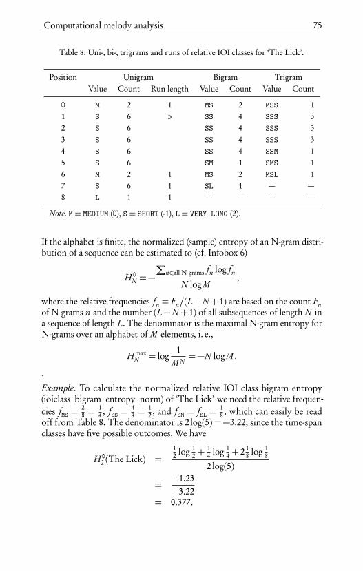
Computational melody analysis 75
Table 8: Uni-, bi-, trigrams and runs of relative IOI classes for ‘The Lick’.
Position Unigram Bigram TrigramValue Count Run length Value Count Value Count
0 M 2 1 MS 2 MSS 11 S 6 5 SS 4 SSS 32 S 6 SS 4 SSS 33 S 6 SS 4 SSS 34 S 6 SS 4 SSM 15 S 6 SM 1 SMS 16 M 2 1 MS 2 MSL 17 S 6 1 SL 1 — —8 L 1 1 — — — —
Note. M = MEDIUM (0), S = SHORT (-1), L = VERY LONG (2).
If the alphabet is finite, the normalized (sample) entropy of an N-gram distri-bution of a sequence can be estimated to (cf. Infobox 6)
H 0N =−
∑
n∈all N-grams fn log fn
N log M,
where the relative frequencies fn = Fn/(L−N +1) are based on the count Fnof N-grams n and the number (L−N + 1) of all subsequences of length N ina sequence of length L. The denominator is the maximal N-gram entropy forN-grams over an alphabet of M elements, i. e.,
H maxN = log
1M N=−N log M .
.
Example. To calculate the normalized relative IOI class bigram entropy(ioiclass_bigram_entropy_norm) of ‘The Lick’ we need the relative frequen-cies fMS =
28 =
14 , fSS =
48 =
12 , and fSM = fSL =
18 , which can easily be read
off from Table 8. The denominator is 2 log(5) =−3.22, since the time-spanclasses have five possible outcomes. We have
H 02 (The Lick) =
12 log 1
2 +14 log 1
4 + 2 18 log 1
8
2 log(5)
=−1.23−3.22
= 0.377.

76 Klaus Frieler
Another important type of sequence features is based on run lengths. A ‘run’in any sequence is a subsequence with only identical elements. Run lengths area natural way of looking at sequences and have several applications, e. g., forstatistical tests or for data compression. For example, in the relative IOI classabstraction of ‘The Lick’ there are four runs of length 1 and one run of length5 (a sequence of eighth notes); see Table 8, Columns 2 and 4. Run lengths canbe used to construct features either as mean lengths of specific elements, e. g.,descending or ascending semitone intervals, or—more generally—as meanrun lengths of all runs of all elements of a certain alphabet as well as derivedconstructions, e. g., ratio_chromatic_sequences, which is the percentage ofchromatic (semitone) passages with respect to all passages, where a passage isdefined as a run of at least three elements.
Structure
Structural features relate to musical form, which is viewed here as the self-similarity of a melody with respect to a given segmentation, e. g., phrases. Toquantize self-similarity for melodies, one needs a melodic similarity measure(Müllensiefen & Frieler, 2004; Frieler, 2009), which is normally conceptual-ized as a (symmetric) map
σ(m1, m2)→ [0,1],
for two melodies m1 and m2 with values in the unit interval, where the value1 is interpreted as ‘identity’ and 0 as maximal dissimilarity. If a segmentationof a melody m into M segments (mi )1≤i≤M is given, then the self-similaritymatrix is given by the values
σi j = σ(mi , m j ).
Currently, in the MeloSpySuite/GUI only interval-based self-similarity matri-ces for bar and phrase segmentations are available and the similarity measureis defined via the edit distance (Müllensiefen & Frieler, 2004). From a self-similarity matrix, scalar features can be derived via statistical descriptors ofdistributions of similarity values, e. g., for adjacent segments or non-adjacentsegments. Using a clustering algorithm to find clusters of segments with highinter-group similarity, the SSM can also be expressed as a form string, e. g.,where similar segments are labeled with letters and primes, e. g., aaba’. (Thisis also available for duration classes.)
Tone formation
Tone formation means the actual process of performing a note (the mapof abstract notes to performed tones). Currently, this falls into three main

Computational melody analysis 77
categories: articulation, f0-modulation, and loudness. Micro-timing as animportant fourth dimension is sorted under rhythm features.
Articulation is traditionally addressed with musical labels such as staccato,legato, portamento etc., which often also have special symbols in commonWestern musical notation, e. g., dots for staccato and horizontal lines forlegato. There are also instrument specific articulations, such as spizzicato forbowed instruments. For our purposes, we approximately define the articu-lation of a tone event simply as the ratio of duration to inter-onset interval.Higher ratios indicate more legato and smaller ones more staccato articulation.This is only a first approximation, e. g., there is an absolute, tempo-dependentaspect to articulation which is ignored when using time-spans ratios—whichare tempo invariant by definition. With this definition, the articulation val-ues with a range of 0 to 1 for monophonic melodies can be easily calculatedfrom the basic representation and scalar global features can be derived usingstatistical descriptors such as mean, median, and standard deviation.
f0-modulation means the changing of the fundamental frequency ( f0) of a tone.The abstraction that a tone event has one single pitch is very often not justifiedin practice, particularly not for wind instruments and singing. Frequently,bends, slides, and vibratos can be observed. Measuring f0-modulations isnot an easy task. The techniques used for the solos in the Weimar Jazz Da-tabase are explained in detail in Chapter Score-informed audio analysis ofjazz improvisation. In the MeloSpySuite/GUI only a basic set of features isavailable, which includes the deviation of the f0 from the nominal 12-toneequal tempered pitch, the vibrato (modulation) frequency and the modulationrange (in cents). Moreover, for the solos in the Weimar Jazz Database manualtone-wise annotations of f0-modulation types are available, which can takeon the values BEND, SLIDE, FALL-OFF, STRAIGHT (no modulation), and theempty value (no annotation).
Loudness and intensity are the third aspect of tone formation. Intensity valuesare not easily measured and the corresponding loudness (a psycho-physicalconcept) even less so. Nevertheless, for each tone event in the Weimar JazzDatabase, intensity estimations were extracted using sophisticated audioalgorithms, as described in detail in Chapter Score-informed audio analysisof jazz improvisation. This results in a frame-wise estimation of intensityvalues per tone, for which the maximum, median, and standard deviationsare available. Furthermore, the relative position of the loudness maximumwith respect to the duration of the tone and the temporal centroid of theframe-wise loudness distribution are provided. Finally, the ratio of the medianloudness to the median value of the background track is included (signal-to-background ratio).

78 Klaus Frieler
Patterns
In the context of jazz research, we are interested in the use of patterns duringimprovisation (e. g., Owens, 1974; Norgaard, 2014). To measure the patterncontent in improvisations, we devised the melpat module of the MeloSpy-Suite/GUI, which helps with two basic tasks in this context: pattern searchand pattern mining/extraction. In the first task, a certain pattern is given andinstances of this pattern are to be found in a corpus of melodies. In the secondtask, all patterns, possibly subject to certain conditions, are to be extractedautomatically from a corpus of melodies.
More specifically, patterns in the context of melodies are defined as subse-quences, or N-grams, of a certain representation of the melody, e. g., intervalor pitch sequences. Therefore, we recall and extend first the notations forsequences and N-grams as introduced earlier (p. 63).
Basic definitions
Our starting point is a corpusC = mi of melodies and a local (point-wise)transformation F with target space TF , so that the object of interest is the setof transformed sequences in the corpusF = si ≡ F (mi ), mi ∈C . For thesake of simplicity, we will write C for a transformed corpus as well.
The maximal length of the corpus is the length of the longest sequence in C ,notated as lmax(C ) =maxs∈C l (s), where l (s) is the length of the sequences . The size of the corpus is the number of sequences in C , notated as σ(C ).The total length of the corpus is the sum of all lengths of all sequences
l∞(C ) =∑
s∈Cl (s).
We denote subsequences of a sequence s with
si : j = (si , si+1, . . . , s j )
for 0≤ i ≤ j < l (s ). The length of the subsequence is l (si : j ) = j − i + 1. Wedenote the set of all subsequences of length n of s as n(s ), e. g., 2(s ) is the setof all bigrams, 3(s) the set of all trigrams of s .
Two sequences are said to be identical if they have the same length and thesame sequence of elements. An N-gram is then the equivalence class of allidentical sequences of length N (over the target space TF ). The standardrepresentative of an N-gram is then the sequence [0 : N − 1] → TF . The

Computational melody analysis 79
frequency of an N-gram n in a sequence s is the size of the set of occurrencesof n in s :
χs (n) = i ∈ [0 : l (s)− 1],where si :i+N−1 = n,
hence, Fs (n) = |χs (x)| . χs (n) is the set of all indices for s where the N-gramn can be found. We say n is contained in s , n ∈ s , if the set of occurrences isnot empty, i. e., χs (n) 6= ;.The relative frequency of n in s is defined as the ratio of frequency to themaximal number of subsequences of length N in s , i. e.,
fs (n) =Fs (n)
l (s)−N + 1,
see Table 8 for an example.
The frequency of an N-gram in a corpusC is the sum of all frequencies of theN-gram over all sequences in the corpus, i. e., the size of the set of occurrencesof n in C :
χC (n) =⋃
s∈Cχs (n).
Hence,FC (n) = |χC (n)|=
∑
s∈CFs (n).
The relative frequency of n in the corpus is then defined as
fC (n) =FC (n)
∑
s∈C l (s)−N + 1.
The number of occurrences of an N-gram n in the corpus is the number ofsequences where n appears at least once, i. e., the size of the set of embeddingsequences:
ωC (n) = s ∈C where n ∈ s.
Pattern search
Pattern search can be defined as searching for a given sequence in a corpus(after suitable transformation). For a given search pattern (N-gram) n in acorpus C , the search result is just the set of subsequences and indices wherethe pattern can be found:
ρC (n) = ( j , i , l (n)) | i ∈ χs j(n) 6= ;.
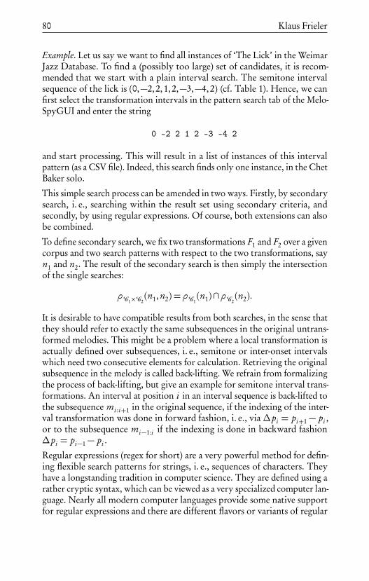
80 Klaus Frieler
Example. Let us say we want to find all instances of ‘The Lick’ in the WeimarJazz Database. To find a (possibly too large) set of candidates, it is recom-mended that we start with a plain interval search. The semitone intervalsequence of the lick is (0,−2,2,1,2,−3,−4,2) (cf. Table 1). Hence, we canfirst select the transformation intervals in the pattern search tab of the Melo-SpyGUI and enter the string
0 -2 2 1 2 -3 -4 2
and start processing. This will result in a list of instances of this intervalpattern (as a CSV file). Indeed, this search finds only one instance, in the ChetBaker solo.
This simple search process can be amended in two ways. Firstly, by secondarysearch, i. e., searching within the result set using secondary criteria, andsecondly, by using regular expressions. Of course, both extensions can alsobe combined.
To define secondary search, we fix two transformations F1 and F2 over a givencorpus and two search patterns with respect to the two transformations, sayn1 and n2. The result of the secondary search is then simply the intersectionof the single searches:
ρC1×C2(n1, n2) = ρC1
(n1)∩ρC2(n2).
It is desirable to have compatible results from both searches, in the sense thatthey should refer to exactly the same subsequences in the original untrans-formed melodies. This might be a problem where a local transformation isactually defined over subsequences, i. e., semitone or inter-onset intervalswhich need two consecutive elements for calculation. Retrieving the originalsubsequence in the melody is called back-lifting. We refrain from formalizingthe process of back-lifting, but give an example for semitone interval trans-formations. An interval at position i in an interval sequence is back-lifted tothe subsequence mi :i+1 in the original sequence, if the indexing of the inter-val transformation was done in forward fashion, i. e., via ∆pi = pi+1− pi ,or to the subsequence mi−1:i if the indexing is done in backward fashion∆pi = pi−1− pi .
Regular expressions (regex for short) are a very powerful method for defin-ing flexible search patterns for strings, i. e., sequences of characters. Theyhave a longstanding tradition in computer science. They are defined using arather cryptic syntax, which can be viewed as a very specialized computer lan-guage. Nearly all modern computer languages provide some native supportfor regular expressions and there are different flavors or variants of regular

Computational melody analysis 81
Table 9: List of special characters for regular expression search.
Special character Meaning
. matches any elementˆ matches beginning of sequence$ matches end of sequence* zero or more repetitions+ one or more repetitions? zero or one repetition
m exactly m repetitionsm,n between m and n repetitions| matches either regex before or after the symbol
expressions. The basic elements for regular expressions are character sets,quantifiers, and position indicators. For instance, the string [a-z] indicatesthe set of lower-case letters in most regex implementations. Wildcards, e. g., asingle dot, which stand in for an arbitrary character are also very important.Examples for quantifiers are *, meaning ‘zero or more instances’, and + for‘one or more instances’. Examples for position parameters are ˆ (‘caret’) for‘beginning of a string’ and $ for ‘end of a string’ (cf. Table 9).
With only these few elements, rather complex search patterns can already bedefined. For example, the regex ˆA[a-z]+C will find all strings that start withan upper-case A, followed by at least one lower-case letter, and an upper-caseletter C. For example. the strings ABC, AAbC, and AC would not match thispattern, but AbC and AabcC would.
Regular expressions are defined for finite alphabets, i. e., ASCII or unicode.To use the powerful regex machinery for melodic sequences, only transfor-mations which have a finite alphabet can be used. For continuous transfor-mations, i. e., inter-onset intervals, they are not applicable. On using regularexpressions with the MeloSpyGUI, see Infobox 7.
Infobox 7: Using regular expressions for pattern search
The use of regular expressions (regex) for finite-sized transformations is donein the MeloSpySuite/GUI by mapping the target domain of the transforma-tion to a consecutive segment in the unicode alphabet and using the regularexpression library for Python. The basic syntax of regular expressions thus

82 Klaus Frieler
follows the Python rules (https://docs.python.org/2/library/re.html). How-ever, this mapping to unicode characters cannot be used for actually inputtingregular expressions, which makes a hybrid syntax necessary. Moreover, usingfixed character classes such as \w, which means all alphanumeric characters(i. e., [a-zA-Z0-9_]) in standard Python regex syntax is of no use. Instead, thestandard representations have to be used to define ‘character sets’ manually. Forexample, for semitone intervals, integer numbers are used, e. g., the sequence-1 0 1 -2 (without commas) means a sequence of a semitone down, a tonerepetition, a semitone up, and a whole-tone down. All quantifiers and positionparameters have to be (singly or doubly) quoted, e. g., ’[’ -1 0 ’]+’ meansone or more occurrences of the elements -1 0 (semitone down and repetition).The most important special characters for the use of regexes in pattern searchcan be found in Table 9.In case of the above example, the interval search for ‘The Lick’, one might thinkthat the first tone repetition could be absent and the last tone could be varied.This can be expressed with the regex
0 "?" -2 2 1 2 -3 -4 "."
This will find variations of ‘The Lick’ with and without the first tone repetition,as expressed by the quantifier ? translating to ‘zero or one tone repetition’, andwith all possible end tones, expressed by the dot . as a stand-in for all possibleintervals. The actual search in the Weimar Jazz Database brings up six instancesof four different patterns: the original instance with the tone repetition at thebeginning, and five beginning with a descending whole tone (-2), two of whichend in a descending fourth (-5) and two in a descending minor third (-3).
Pattern mining
The task of pattern mining or pattern extraction is to extract all patterns froma given corpus C , which is subject to certain conditions for the patterns.A pattern database with minimal length K , maximal length M is the setof all N-grams with k ≤ N ≤ M . Often, we like to subject the patterndatabase to further conditions, e. g., minimal frequencies or occurrences. Infact, (sequential) patterns are often defined as N-grams that occur at least ktimes in at least l different entities in the corpus, with the minimal definitionof K = 2 and L= 1. Obviously, L≥ 1 implies also K > 1.
Another useful restriction, available as a submodule to the melpat module inthe MeloSpySuite/GUI, is called pattern partition. A pattern partition is de-fined for a single sequence s in the corpus with respect to the pattern databaseof the entire corpus (including the borderline case of a single-sequence corpus).
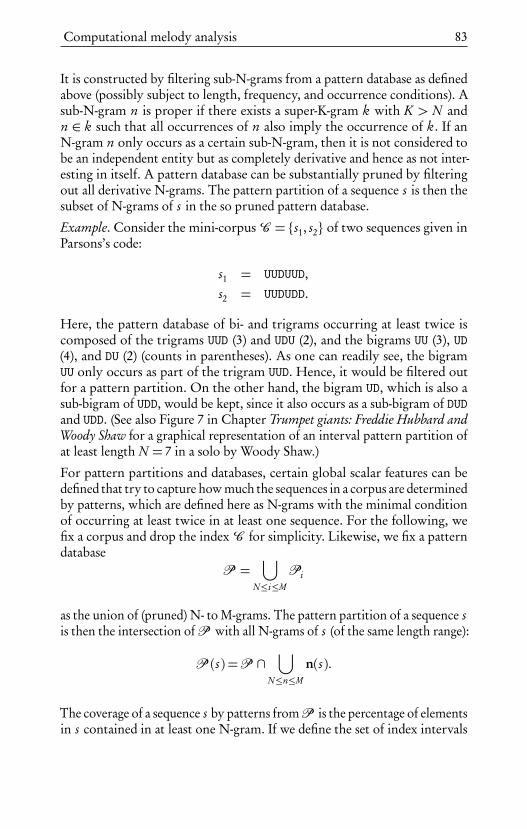
Computational melody analysis 83
It is constructed by filtering sub-N-grams from a pattern database as definedabove (possibly subject to length, frequency, and occurrence conditions). Asub-N-gram n is proper if there exists a super-K-gram k with K > N andn ∈ k such that all occurrences of n also imply the occurrence of k. If anN-gram n only occurs as a certain sub-N-gram, then it is not considered tobe an independent entity but as completely derivative and hence as not inter-esting in itself. A pattern database can be substantially pruned by filteringout all derivative N-grams. The pattern partition of a sequence s is then thesubset of N-grams of s in the so pruned pattern database.
Example. Consider the mini-corpus C = s1, s2 of two sequences given inParsons’s code:
s1 = UUDUUD,s2 = UUDUDD.
Here, the pattern database of bi- and trigrams occurring at least twice iscomposed of the trigrams UUD (3) and UDU (2), and the bigrams UU (3), UD(4), and DU (2) (counts in parentheses). As one can readily see, the bigramUU only occurs as part of the trigram UUD. Hence, it would be filtered outfor a pattern partition. On the other hand, the bigram UD, which is also asub-bigram of UDD, would be kept, since it also occurs as a sub-bigram of DUDand UDD. (See also Figure 7 in Chapter Trumpet giants: Freddie Hubbard andWoody Shaw for a graphical representation of an interval pattern partition ofat least length N = 7 in a solo by Woody Shaw.)
For pattern partitions and databases, certain global scalar features can bedefined that try to capture how much the sequences in a corpus are determinedby patterns, which are defined here as N-grams with the minimal conditionof occurring at least twice in at least one sequence. For the following, wefix a corpus and drop the index C for simplicity. Likewise, we fix a patterndatabase
P =⋃
N≤i≤M
Pi
as the union of (pruned) N- to M-grams. The pattern partition of a sequence sis then the intersection ofP with all N-grams of s (of the same length range):
P (s) =P ∩⋃
N≤n≤M
n(s).
The coverage of a sequence s by patterns fromP is the percentage of elementsin s contained in at least one N-gram. If we define the set of index intervals

84 Klaus Frieler
in s where any n covered by any N-gram fromP as
Γ (s) = i , . . . , i +N − 1 | ∃n∈P : i ∈ χs (n),
then the coverage is simply
γ (s) =|Γ (s)|l (s)
.
The over coverage is the average number of N-grams to which an element in sbelongs. The average overlap is defined as the average number of elements twoadjacent patternsP share, where the patterns are sorted with respect to startpositions in s . The average N-gram length is defined as the mean length ofN-grams contained in the pattern partition of s . Finally, the mean logarithmexcess probability is defined using the ratio of the observed frequency of apattern to the expected frequency derived from a Markov process of zerothorder. The latter is just a complicated term for the product of the probabilitiesof the elements that constitute an N-gram. For an illustration, consider themini-corpus of Parsons’s code sequences from above. The relative frequenciesof the unigrams are fU =
712 and FD =
512 . Using elementary probability
theory, the a priori frequency is the probability under the assumption thatall elements in the sequence are independently produced, i. e., the product ofthe single probabilities. The trigram UUD thus has an expected probability of
pe (UUD) = p(U)p(U)p(D) =712· 7
12· 5
12= 0.142.
On the other hand, the observed frequency is three times out of a possibleeight times, or po =
38 = 0.375. The ratio of observed to expected probabilities,
the excess probability, is then
po
pe=
0.3750.142
= 2.64.
Hence the trigram UUD appears about 2.6 times more often than an indepen-dent (Markov) process would suggest. The logarithm of excess probabilityis then used to make the process of averaging excess probabilities over allpatterns more meaningful.
Statistical feature selection:searching for musical style
Martin Pfleiderer and Jakob Abeßer
The Weimar Jazz Database offers myriads of possibilities to compare vari-ous subsets of data using musical features which are automatically extractedwith MeloSpyGUI and statistical methods. In the following pilot study, onepowerful statistical approach is chosen. It follows a simple idea: First, thedatabase is divided into two subsets, e. g., the improvisations of a certain mu-sician versus the improvisations of all other musicians, or all improvisationswithin one jazz style or played with a certain musical instrument versus allremaining improvisations. Next, the statistical values for a large number ofmusical features are automatically extracted for these two subsets. In the laststep, those musical features that differ significantly between the two subsetsare identified. In a statistical sense, these discriminative features can be in-terpreted as being particular or idiosyncratic for a musical characterizationof the chosen subset, e. g., for the improvisations of a certain musician—atleast in regard to those improvisations which are included in the Weimar JazzDatabase. From these exploratory findings with regard to the particularitiesof certain musicians, jazz styles, or instruments, one can confirm or questionexisting claims about jazz styles as well as gain new insights into stylisticfeatures within the history of jazz which, in turn, could be further examinedwith subsequent analytical case studies.
Within the 456 solos included in the Weimar Jazz Database, there are, how-ever, only few musicians who are represented with more than five or siximprovised solos. To expand the statistical base for the method, chorusesinstead of entire solos were chosen as basic investigation units, resulting inan extended corpus of 1416 (chorus) units. Thus, longer solos with manychoruses receive more weight, while short solos with only a few choruses
86 Martin Pfleiderer and Jakob Abeßer
receive less weight. Likewise, however, improvisations with an open form,e. g., the solos of Ornette Coleman, also receive less weight.
For each of the 1416 choruses, 121 statistical values concerning various musi-cal features were extracted. All statistical values discussed below were averagedover all investigation units of the subsets of interest. The features encompassseveral musical dimensions:
• Pitch: Extended chordal pitch classes are chosen, since this category isvery relevant in a jazz improvisation context by relating pitch classesto each underlying chord. Additionally, there are several values con-cerning the overall range of pitch usage and the degree of chromaticity,as well as the entropy of the usage of pitches and pitch classes, e. g.,how redundant (low entropy value) or unforeseeable (high entropyvalue), resp., the usage of pitch classes is within the improvisation.
• Interval: The usage of intervals is characterized by interval classes (fuzzyintervals) and several statistical values including interval entropy, range,and mean.
• Rhythm and meter: Rhythm is characterized by several measures ofduration classes and classes of inter-onset intervals in regard to bothtempo and absolute time (seconds). Moreover, there are general mea-sures for event density and tempo. Meter is characterized by variousmeasures, e. g., by syncopicity, metrical complexity, and entropy.
• Lines: The characteristics of longer lines are depicted, among others,by the mean lengths of ascending and descending passages, chromaticlines, and arpeggios. By measuring the run-lengths of identical dura-tion classes or interval classes, one can characterize the uniformity ofthe improvised line, e. g., if a musician mainly plays eighth-chains ofdescending steps.
Sometimes, several statistical values indicate the same musical feature in aslightly different way, e. g., the event density in regard to the tempo or inregard to absolute time intervals in seconds. Some of those features are alreadyexplained in Chapter Computational melody analysis, others are introducedin this chapter during the interpretation of the results. The exact definitionsof all features are documented with their corresponding feature definitionfiles, which are listed in regard to musical parameters within the onlinedocumentation.12
12http://jazzomat.hfm-weimar.de/commandline_tools/melfeature/melfeature_features.html

Statistical feature selection 87
In an exploratory study, the subsets of the data are built following the cat-egories ‘performer’, ‘style’, ‘tonality type’, and ‘instrument’. This resultsin several dozens of statistical investigations comparing each musician withall other musicians, each style (traditional, swing, bebop, cool/West Coast,hardbop, postbop, fusion, free) with all other styles, each tonality type (‘func-tional’, ‘blues’, ‘modal’, ‘color’ and ‘free’) with all other types and eachmusical instrument with all other instruments. However, to gain meaningfulresults, it is important that the size of a subset is not too small, since com-paring just two choruses with the remaining 1414 choruses of the WeimarJazz Database will evidently not lead to statistically robust and conclusivefindings.
In order to identify those musical features that discriminate the two datasubsets significantly, the statistical method of classification or decision treeswas chosen (Breiman, 2001). Given a two-class partition of the dataset, arandom forest classifier with 250 decision trees was trained using randomsubsets of both investigation units (choruses) and features, since this approachleads to more robust classification models.
As a next step, the 20 features with the highest differences between thetwo subsets were selected. For each of those features a two-sample t-testwas performed in order to investigate whether the distribution means ofboth subsets for a particular feature differ significantly in a statistical sense.Furthermore, the Cohen’s d effect size measure (Cohen, 1988) was computedin order to determine how big the difference between the subsets effectivelyis. Finally, all features with a significant difference of means ( p < 0.05) and arather strong effect size of d > 0.5 were selected. The ranking of the chosenmusical features in the tables results from the absolute values of this effect size.However, due to space constraints, in the following only a small selection ofthe results are reported and interpreted in order to give just an impressionof the potentials of the statistical procedure. The discussion is confined tosome of the most striking examples in regard to the performers’ personalstyle as well as to jazz style, harmonic style and instrument, respectively.The complete lists of features concerning all subsets are stored in an onlinerepository13 and are open for examination.
Characteristics of jazz style, tonality type and instrument
Could jazz styles be differentiated in regard to how jazz musicians improvisewithin these styles? Surprisingly, there are no statistical differences between
13https://github.com/jazzomat/python/tree/master/publications/book_2017/feature_selection

88 Martin Pfleiderer and Jakob Abeßer
Table 1: Significant features of improvisations within swing style (106 choruses)compared to all other improvisations (1310 choruses).
Feature Mean (class) Mean (others) Cohen’s d Sig.
ioiclass_abs_hist_01_very_short 0.306 0.452 −0.60 ***durclass_abs_hist_02_short 0.408 0.302 0.52 ***ioiclass_abs_hist_02_short 0.494 0.387 0.52 ***
the subsets of all solos stylistically labeled as ‘bebop’, ‘cool’ or ‘hardbop’ andthe respective remaining solo corpus. Apparently, the ways in which jazzmusicians improvise within these modern jazz styles of the 1940s and 1950sare similar to a degree that makes it impossible to distinguish between themon a global statistical level. One could conclude that bebop, cool jazz andhardbop all lie at the core of jazz improvisation as represented within theWeimar Jazz Database.
Looking at the jazz styles beyond this modern ‘common practice jazz’, the sta-tistically most significant differences lie within the domain of rhythm and du-ration rather than pitch and harmony. Looking, for example, at all 106 swingchoruses in contrast to the remaining 1310 choruses improvised in other jazzstyles (Table 1), there are only three distinguishing measures that are statisti-cally significant and have a strong effect size: Swing solos have fewer ‘veryshort’ duration intervals (31 % vs. 45 %, durclass_abs_hist_01_very_short)and a much higher percentage of both ‘short’ durations (41 % vs. 30 %, dur-class_abs_hist_02_short) and ‘short’ inter-onset intervals (49 % vs. 39 %,ioiclass_abs_hist_02_short), both in regard to absolute time, i. e., indepen-dent from tempo. Generally speaking, swing musicians play ‘slower’ lines(i. e., with more eighth notes and fewer sixteenth notes) than the players inthe remaining corpus. The same holds true for musicians playing traditionaljazz. In contrast, postbop musicians play a much higher percentage of ‘veryshort’ durations and inter-onset intervals, i. e., ‘faster’ lines.
Some jazz styles are tied to certain tonality types. Improvisations withinfunctional tonality, blues tonality and ‘color’ tonality (defined as mainlynon-functional chord changes employed in postbop or fusion jazz) displaysignificant differences compared to the respective remaining improvisationsonly with regard to interval range (blues uses smaller intervals) and pitchrange (higher within ‘color’ tonality). However, modal improvisations havemany significant differences compared to all other, non-modal improvisationsincluding those pieces classified as ‘color’ (Table 2). In the Weimar JazzDatabase, there are 102 choruses of modal improvisation taken from 25solos. Within those solos, there are fewer minor thirds (‘blue notes’) played

Statistical feature selection 89
Table 2: Significant features of improvisations with modal tonality (102 choruses)compared to all other improvisations (1314 choruses).
Feature Mean (class) Mean (others) Cohen’s d Sig.
int_range 29.500 21.068 0.93 ***abs_int_range 17.225 12.38 0.84 ***cdpcx_density_> 0.029 0.011 0.83 ***int_std 4.007 3.33 0.76 ***ioiclass_abs_hist_02_short 0.267 0.405 −0.67 ***cdpcx_density_B 0.008 0.036 −0.63 ***durclass_abs_hist_02_short 0.199 0.318 −0.59 ***abs_int_mean 3.017 2.661 0.58 ***ioiclass_abs_hist_01_very_short 0.570 0.431 0.57 ***pitch_std 5.946 5.038 0.56 ***durclass_abs_entropy 0.475 0.593 −0.54 ***
over major scales or chords than within the remaining corpus (0.8 % vs.3.6 %, cdpcx_density_B). Moreover, there are significantly fewer major thirdsplayed over minor chords or scales (dorian, aeolian, phrygian, locrian) thanwithin the remaining corpus (1.1 % vs. 2.9 %, cdpcx_density_>). While thepercentage of these dissonant pitches is in general very low, those dissonancesare clearly avoided within modal improvisation. Additionally, there is ahigher range of intervals used within modal improvisation (see int_rangeand abs_int_range), and there are more ‘very short’ tone durations than‘short’ tone durations (shown with significant differences with regard toioiclass_abs_hist_02_short, durclass_abs_hist_02_short and ioiclass_abs_hist_01_very_short)—which is significant also for postbop in general.
With regard to musical instruments, improvisations played on the trombonedisplay the most significant differences compared with improvisations playedon all other instruments (Table 3). Included in the subset are 76 trombonechoruses within 26 solos played by stylistically diverse jazz musicians, suchas Kid Ory, Dickie Wells, J. J. Johnson, Curtis Fuller, or Steve Turre. Thesedifferences include a higher share of medium inter-onset intervals relativeto tempo (31 % vs. 16 %, ioiclass_rel_hist_03_medium), a higher metricalcomplexity (0.22 vs. 0.17 for metric_complexity, and 0.17 vs. 0.10 for met-ric_complexity_compression) as well as a significantly higher percentage oftone repetitions (12 % vs. 5 % of all played intervals, fuzzyint_hist_05_repeat).Therefore, trombone players clearly play slower, but metrically more com-plex lines with much more tone repetitions than musicians improvising onother instruments.

90 Martin Pfleiderer and Jakob Abeßer
Table 3: Significant features of improvisations played on the trombone (76 choruses)compared to all other improvisations (1340 choruses).
Feature Mean (class) Mean (others) Cohen’s d Sig.
ioiclass_rel_hist_03_medium 0.305 0.163 1.11 ***art_median 0.776 0.849 −1.05 ***fuzzyint_hist_05_repeat 0.123 0.053 0.81 ***parsons_hist_constant 0.123 0.053 0.81 ***pitch_median 61.736 65.607 −0.78 ***metric_complexity 0.221 0.167 0.77 ***art_std 0.214 0.185 0.72 ***ric_mean_seg_len 1.811 2.320 −0.63 ***aic_mean_seg_len 1.698 2.314 −0.61 ***metric_complexity_compression 0.166 0.101 0.59 ***parsons_entropy 0.822 0.711 0.57 ***metric_complexity_division 0.276 0.232 0.56 ***pitch_range 18.934 23.461 −0.55 ***pitch_std 4.258 5.151 −0.54 ***parsons_bigram_entropy 2.485 2.168 0.53 ***
By contrast, improvisations played on the alto saxophone seem to lie rightin the center of our database (with no significant differences to the rest ofthe database), while tenor saxophone and trumpet solos mainly differ withregard to pitch range (tenor is lower, trumpet is higher) as well as in the caseof trumpet solos with regard to the share of very long tones (2.9 % vs. 1.7 %,ioiclass_rel_hist_05_very_long).
Personal style of jazz musicians
Each jazz musician improvises on a variety of pieces exhibiting a variety ofdifferent chord changes, differing tempos and differing rhythmic feels. Despitethese many different contexts and frameworks for improvisation, are thereany musical peculiarities which, in general, differentiate the improvisationsof one jazz musician from those of all other jazz musicians? Presumably,the issue of personal style is one of the most exciting topics with regard tojazz improvisation. Looking at the many results provided by our statisticalapproach, the answer seems to be ambivalent: On the one hand, there aresignificant differences between the solos of almost every jazz musician andthe remaining corpus. But on the other hand, there are fewer differencesthan expected—and sometimes the significant differences are rather trivial,e. g., that a trumpet player’s improvisations shows a higher and a baritonesaxophonist show a lower mean pitch due to the tonal range of the instrument.

Statistical feature selection 91
Table 4: Significant features of improvisations played by Benny Goodman (8 choruses)compared to all other improvisation (1408 choruses).
Feature Mean (class) Mean (others) Cohen’s d Sig.
durclass_rel_hist_04_long 0.156 0.028 1.55 ***pitch_median 72.312 65.360 1.39 ***avgtempo 264.900 194.667 1.00 **mean_length_chromatic_descending 4.562 2.896 0.98 **mean_length_chromatic_mixed 4.657 3.542 0.89 *syncopicity 0.191 0.314 0.87 *int_min −14.250 −10.020 −0.78 *mean_length_arpeggio_ascending 3.713 2.598 0.76 *mean_length_chromatic_sequences 4.171 3.177 0.74 *mean_length_arpeggio_descending 3.558 2.541 0.72 *
In some cases, however, the statistical approach yields results which shouldbe further examined. Here are five examples.
Swing clarinetist Benny Goodman is included in the Weimar Jazz Data-base with only seven solos and eight choruses. Goodman plays more longarpeggios, both ascending (3.7 tones vs. 2.6 tones on average, seemean_length_arpeggio_ascending) and descending (3.6 tones vs. 2.6 tones on average,mean_length_arpeggio_descending), more long chromatic sequences (4.2 vs.3.2 tones on average, mean_length_chromatic_sequences) as well as morelong tones relative to the beat (15.6 % vs. 2.8 %, durclass_rel_hist_04_long)(Table 4). Moreover, his improvisations display a smaller amount of synco-pated tones (19 % vs. 31 % of all tones, syncopicity) than the improvisationsof the other musicians. Unfortunately, all solos by Goodman in the WeimarJazz Database are in a fast or very fast tempo (199 to 303 bpm). Therefore, itis disputable whether the significant features which distinguish Goodman’simprovisations from all other improvisations are indeed peculiarities of hisgeneral personal style or are just due to the fast tempo. In particular, a highvalue for syncopicity could result from playing inaccuracies, e. g., tones playedtoo early (or too late), which are detected as syncopations.
The next four examples are all related to postbop improvisation. Beside beingplayed higher (as with all trumpet players) and faster (as with all postbop mu-sicians), Woody Shaw’s improvisations differ from all other improvisationsby rather high percentages of fourths (11.2 % vs. 8.5 %, cdpcx_density_4) andminor seconds (5.5 % vs. 3.9 %, cdpcx_density_b2) in regard to the underlyingharmony (see Table 5). By contrast, tenor saxophonist Wayne Shorter dis-plays peculiarities in regard to choice of pitches (see Table 6): Compared withthe improvisations of all the other musicians, he has a slightly but significantly

92 Martin Pfleiderer and Jakob Abeßer
Table 5: Significant features of improvisations by Woody Shaw (23 choruses) comparedto all other improvisations (1393 choruses).
Feature Mean (class) Mean (others) Cohen’s d Sig.
pitch_median 71.326 65.301 1.21 ***ioiclass_rel_hist_01_very_short 0.607 0.438 0.68 **cdpcx_density_4 0.112 0.085 0.59 **cdpcx_density_b2 0.055 0.039 0.55 **
Table 6: Significant features of improvisations by Wayne Shorter (34 choruses) com-pared to all other improvisations (1382 choruses).
Feature Mean (class) Mean (others) Cohen’s d Sig.
art_std 0.216 0.185 0.75 ***cdpcx_density_> 0.027 0.012 0.72 ***cdpcx_density_T 0.064 0.042 0.50 **
higher preference for playing tritones (6.4 % vs. 4.2 %, cdpcx_density_T) aswell as major thirds over minor chords (2.7 % vs. 1.2 %, cdpcx_density_>).
David Liebman is a postbop saxophone player who reflected his individualapproach to improvisation in several texts, including a comprehensive treatisecalled A Chromatic Approach to Jazz Harmony and Melody (Liebman 1991).Therefore, in regard to the improvisations included in the Weimar Jazz Da-tabase, one could ask to what degree he puts his chromatic approach intopractice. In regard to the ten musical features which significantly differentiateLiebman’s solos from all other solos, there are three features concerningchromaticity and another three features concerning the usage of non-diatonicintervals (Table 7). The mean length of both chromatic sequences and de-scending chromatic lines is higher within Liebman’s solos than within othersolos (3.9 vs. 3.2 tones, mean_length_chromatic_sequences, and 4.2 vs. 2.9tones, mean_length_chromatic_descending) as well as the mean length ofsequences with both ascending and descending semitones (which includetrills, mean_length_chromatic_mixed). Liebman uses significantly more tri-tones (7.5 % vs. 4.2 %, cdpcx_density_T), minor seconds (6.1 % vs. 3.8 %,cdpcx_density_b2) and minor sevenths over major chords (0.8 % vs. 0.2 %,cdpcx_density_<) than the other musicians. Of course, chromaticity anddissonant pitches are interrelated. Additionally, both the pitch entropy (4.3vs. 3.8, pitch_entropy) and standard deviation of pitch usage (6.3 vs. 5.1,pitch_std) are higher. It is remarkable that both pitch entropy and pitch stan-

Statistical feature selection 93
Table 7: Significant features of improvisations by Dave Liebman (34 choruses) com-pared to all other improvisations (1382 choruses).
Feature Mean (class) Mean (others) Cohen’s d Sig.
cdpcx_density_T 0.075 0.042 0.79 ***mean_length_chromatic_descending 4.193 2.874 0.78 ***cdpcx_density_b2 0.061 0.038 0.77 ***pitch_std 6.314 5.073 0.76 ***pitch_median 68.852 65.314 0.71 ***cdpcx_density_< 0.008 0.002 0.59 ***pitch_entropy 4.313 3.763 0.57 ***mean_length_chromatic_sequences 3.906 3.164 0.55 **mean_length_chromatic_mixed 4.216 3.532 0.54 **
Table 8: Significant features of improvisations by Dave Liebman (34 choruses) com-pared to all improvisations labeled as “postbop” and played on the tenor saxophone(513 choruses).
Feature Mean (class) Mean (others) Cohen’s d Sig.
pitch_median 68.852 63.633 1.31 ***pitch_std 6.314 5.383 0.55 **ratio_chromatic_sequences 0.125 0.082 0.54 **cpc_bigram_entropy 5.909 5.216 0.51 **pitch_entropy 4.313 3.859 0.51 **
dard deviation are also higher in Liebman’s improvisations than in the impro-visations of all other postbop tenor saxophone solos (Table 8). Compared tothat subset of the database, Liebman’s improvisations show a higher percent-age of chromatic sequences (12.5 % vs. 8.2 %, ratio_chromatic_sequences) anda higher entropy of chordal pitch classes (5.9 % vs. 5.2 %, cpc_bigram_entropy).However, the usage of dissonant non-diatonic pitches does not differ signifi-cantly for Liebman and other postbop tenor saxophone players.
According to the results of the statistical comparisons, trumpet player FreddieHubbard is one of the jazz musicians whose improvisations differ over a ratherbroad variety of musical dimensions (Table 9). While playing more very longtones than the other musicians (in regard to absolute inter-onset intervals,2.5 % vs. 0.6 %, ioiclass_abs_hist_05_very_long), sequences of very shorttones played by Hubbard tend to be longer. The average length of lines withthose ‘very short’ tones is 4.5 tones in Hubbard’s improvisations, while onlybeing 2.3 tones within the remaining corpus (mean_seg_len_01_very_short).In general, the event density is lower within Hubbard’s improvisations (3.4
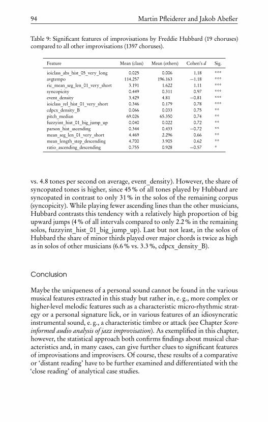
94 Martin Pfleiderer and Jakob Abeßer
Table 9: Significant features of improvisations by Freddie Hubbard (19 choruses)compared to all other improvisations (1397 choruses).
Feature Mean (class) Mean (others) Cohen’s d Sig.
ioiclass_abs_hist_05_very_long 0.025 0.006 1.18 ***avgtempo 114.257 196.163 −1.18 ***ric_mean_seg_len_01_very_short 3.191 1.622 1.11 ***syncopicity 0.449 0.311 0.97 ***event_density 3.429 4.81 −0.81 ***ioiclass_rel_hist_01_very_short 0.346 0.179 0.78 ***cdpcx_density_B 0.066 0.033 0.75 **pitch_median 69.026 65.350 0.74 **fuzzyint_hist_01_big_jump_up 0.040 0.022 0.72 **parson_hist_ascending 0.344 0.433 −0.72 **mean_seg_len_01_very_short 4.469 2.296 0.66 **mean_length_step_descending 4.700 3.905 0.62 **ratio_ascending_descending 0.755 0.928 −0.57 *
vs. 4.8 tones per second on average, event_density). However, the share ofsyncopated tones is higher, since 45 % of all tones played by Hubbard aresyncopated in contrast to only 31 % in the solos of the remaining corpus(syncopicity). While playing fewer ascending lines than the other musicians,Hubbard contrasts this tendency with a relatively high proportion of bigupward jumps (4 % of all intervals compared to only 2.2 % in the remainingsolos, fuzzyint_hist_01_big_jump_up). Last but not least, in the solos ofHubbard the share of minor thirds played over major chords is twice as highas in solos of other musicians (6.6 % vs. 3.3 %, cdpcx_density_B).
Conclusion
Maybe the uniqueness of a personal sound cannot be found in the variousmusical features extracted in this study but rather in, e. g., more complex orhigher-level melodic features such as a characteristic micro-rhythmic strat-egy or a personal signature lick, or in various features of an idiosyncraticinstrumental sound, e. g., a characteristic timbre or attack (see Chapter Score-informed audio analysis of jazz improvisation). As exemplified in this chapter,however, the statistical approach both confirms findings about musical char-acteristics and, in many cases, can give further clues to significant featuresof improvisations and improvisers. Of course, these results of a comparativeor ‘distant reading’ have to be further examined and differentiated with the‘close reading’ of analytical case studies.

Statistical feature selection 95
There are many more possibilities for creating data subsets and examining thedistinguishing musical features of those subsets (cf. p. 175, where differentsubsets of cool jazz players are compared). One could create subgroups of jazzmusicians according to various criteria, e. g., year of birth, origin, affiliation toa certain school or direction, or alleged influence, and then identify the mostdiscriminative features of their improvisations. Or one could also compareimprovisations within certain keys—say, all flat keys against all sharp keys—or tempo ranges in order to gain insights into learning and playing routinesof jazz musicians. Moreover, there are statistical methods for identifying thedifferences between more than two classes. Additionally, one can chooseless restrictive statistical criteria (higher significance threshold, lower effectsize) for the selection of a larger set of relevant musical features, since theseless robust features could also, nonetheless, both carry musical meaningand inspire further investigations and analytical case studies. However, ifthe reader gains some ideas of how to pursue this approach in regard tocertain research issues, the aim of this chapter will be fulfilled—that is, todemonstrate some of the potentials of performing comparative music analysiswith statistical methods.


Score-informed audio analysisof jazz improvisation
Jakob Abeßer and Klaus Frieler
One main challenge of analyzing recordings of ensemble music with compu-tational tools is the inherent overlap of simultaneously sounding instruments.In particular, spectrograms of mixed audio tracks exhibit both horizontalstructures (overtones) and vertical structures (tone attack transients), whichoften superimpose each other (M. Müller, 2015). Separating of a musicianimprovising within an ensemble is very complicated and in many cases im-possible. Furthermore, the sound quality of many audio recordings, e. g., theearly recordings of the transcriptions within the Weimar Jazz Database, israther poor since they come from the early stage of audio recordings in thebeginning of the 20th century.
We face these challenges using a score-informed analysis approach, i. e., weuse the manually created transcriptions of the Weimar Jazz Database (cf.p. 19) of the soloists’ melodies as additional cues during different steps of theaudio analysis. p. 101 will detail how manual transcriptions of pitch, onset,and duration allow for an automatic separation of the ensemble recordinginto two audio streams: the isolated solo instrument and the accompanyinginstruments (rhythm section), respectively. This approach allows for an in-vestigation of the audio recordings of jazz solos in regard to performancefeatures such as dynamics (changes in intensity), intonation (pitch accuracywith respect to a given tone system), articulation (relation of tone durationto inter-onset interval), pitch modulation (temporal variation of the funda-mental frequency over the tone duration) as well as timbre characteristics(sound).
The methods and results discussed in this chapter are complementary tothe symbolic music analysis methods discussed in Chapter Computationalmelody analysis. Following this approach, we pursued several in-depth studies

98 Jakob Abeßer and Klaus Frieler
Figure 1: Score-informed audio analysis of jazz solos.
of the original audio recordings of the solos included in the Weimar Jazz Data-base which are motivated by jazz research questions and which we approachusing several methods from audio signal processing and Music InformationRetrieval (MIR).
Besides analyzing extracted solo parts, we also developed a new algorithm forthe automatic transcription of the bass lines, based on a deep neural network.This representation measures the likelihood of different bass pitch valuesover time and can be used as a first step towards a transcription of walkingbass lines as we show in p. 123.
The score-informed analysis procedure is summarized in Figure 1. At first,the transcribed part of the original audio recording is separated into a backingtrack, which includes the accompanying instruments, and a solo track, whichincludes the improvising soloist (cf. p. 101). Then, the underlying tuningfrequency is estimated from the backing track (cf. p. 101). In the next step, weestimate tone-wise fundamental frequency contours and intensity contoursfrom the isolated solo instrument track (cf. p. 104 and p. 109). Finally, wedescribe each contour using more abstract features such as the fundamentalfrequency modulation range or the median tone intensity (cf. p. 104).

Score-informed audio analysis 99
Table 1: Overview of performers, instrument(s), number of solos, and number oftones.
Performer Instrument # Solos # Tones
Art Pepper as, cl 6 3634Ben Webster ts 5 1826Benny Carter as 7 2650Benny Goodman cl 7 1144Bix Beiderbecke cor 5 680Bob Berg ts 7 4894Branford Marsalis ts 6 4691Cannonball Adderley as 5 2642Charlie Parker as 17 5672Chet Baker tp 8 1428Chris Potter ts 7 7156Clifford Brown tp 9 4232Coleman Hawkins ts 6 2609David Liebman ss, ts 11 7518David Murray ts 6 3005Dexter Gordon ts 6 4149Dickie Wells tb 6 870Dizzy Gillespie tp 6 1808Don Byas ts 8 2264Don Ellis tp 6 1458Eric Dolphy as, bcl 6 3330Fats Navarro tp 6 1968Freddie Hubbard tp 6 2222Gerry Mulligan bs 6 2621Hank Mobley ts 4 2118Herbie Hancock p 5 2769J. J. Johnson tb 8 3324Joe Henderson ts 8 4930Joe Lovano ss, ts, ts-c 8 6104John Coltrane ss, ts 20 19428Johnny Dodds cl 6 722

100 Jakob Abeßer and Klaus Frieler
Performer Instrument # Solos # Tones
Joshua Redman ts 5 2422Kenny Dorham tp 7 2856Kid Ory tb 5 319Lee Konitz as 8 3519Lee Morgan tp 4 2243Lester Young ts 7 1787Lionel Hampton vib 6 1326Louis Armstrong cor, tp 8 1157Michael Brecker ts 10 7601Miles Davis tp 19 6734Milt Jackson vib 6 2302Ornette Coleman as 5 2857Pat Metheny g 4 2374Paul Desmond as 8 2169Pepper Adams bs 5 2343Phil Woods as 6 2802Roy Eldridge tp 6 1748Sidney Bechet ss 5 1078Sonny Rollins ts 13 5399Sonny Stitt as, ts 6 1759Stan Getz ts 6 3705Steve Coleman as, ss 10 5552Steve Lacy ss 6 2332Wayne Shorter ts 10 3815Woody Shaw cor, tp 8 3193Wynton Marsalis tp 7 3070Zoot Sims ts 6 1136
Total 423 191464
In each of the following sections, we describe for each processing step boththe applied computational method and an exemplary corpus study to demon-strate the analytical potentials of our approach. Of course, there are many
Score-informed audio analysis 101
more research issues that could be approached within this analytical frame-work. Most of the data used in the case studies is included within the WeimarJazz Database and is ready to be further explored.
In order to have a representative corpus in regard to personal styles, we focuson all soloists featured within the Weimar Jazz Database with at least foursolos. This selection still covers around 95 % of all annotated tones within theWeimar Jazz Database. Table 1 gives an overview over the selected performersand their instruments as well as the total number of solos and tones for eachperformer.
Source separation
The main goal of the sound source separation step is to isolate the solo in-strument from the accompanying instruments, i. e., the rhythm section. Thealgorithm applied for solo and accompaniment source separation was origi-nally proposed in E. Cano, Schuller, & Dittmar, 2014. The high-quality solotranscriptions from the Weimar Jazz Database, which are perfectly alignedto the audio track, are used as prior information to the separation algorithm.The main approach is to iteratively model the tones of the solo instrumentin the spectral domain. Typical characteristics such as inharmonicity (devi-ation of harmonic frequencies from integer multiples of the fundamentalfrequency), magnitude and frequency smoothness, as well as common ampli-tude modulation among partials are taken into account.
Tuning estimation
Tuning refers to the adjustment of the pitch frequencies of musical instru-ments to a given reference frequency. As will be shown in p. 102, jazz record-ings exhibit a high variance with respect to the tuning frequency. While thefirst jazz recordings date back to the 1920s, a standardized reference frequencyfor the concert pitch A4 of 440 Hz was not defined until 1955 in the ISO 16standard and later re-affirmed in ISO16:1975 (1975). Furthermore, pianos—the most important accompaniment instruments in jazz recordings—tendto detune over time (Fletcher & Rossing, 1998). A third reason for tuningfrequency deviations in early jazz recordings lies in technical imperfectionsin the recording process, such as speed variations in gramophones or taperecorders (Ballou, 2008). As a consequence, the tuning frequency fref must beestimated before the intonation of jazz soloists in relation to the performingensemble can be analyzed. Rhythm section instruments like the piano anddouble bass provide a suitable tuning reference for the soloist since they have

102 Jakob Abeßer and Klaus Frieler
mostly stable tone pitches. Therefore, we estimate fref exclusively from thebacking track, which is automatically extracted using a source separationalgorithm (cf. p. 101). Audible artifacts from the source separation processdo not affect the tuning frequency estimation (Abeßer et al., 2015). An esti-mate of the tuning frequency from the rhythm section allows to investigatewhether and to what extent a soloist tends to play “sharp” or “flat” by usingslightly higher or lower pitch frequencies, respectively.
In a previous study (Abeßer, Frieler, Cano, Pfleiderer, & Zaddach, 2017),we compared two state-of-the-art methods for tuning frequency estimationproposed by Müller and Ewert (2011), as well as Mauch (2010) for tuningfrequency estimation from jazz recordings. In the first approach, a multi-rate filter bank with semitone spacing is used. The center frequencies ofthe filters are systematically shifted in order to estimate the most likelytuning frequency from the averaged spectrogram. In the second approach, anote saliency representation is computed with a third-of-semitone spacing.This saliency is averaged over the full audio recording and analyzed using aDiscrete Fourier Transformation (DFT). The most likely tuning deviationfrom 440 Hz is finally estimated from the phase of the DFT. Both methodsshowed a very high agreement over the solos in the Weimar Jazz Databasewith a sample correlation of r = 0.96 (p < .001). We finally decided touse the method proposed by Mauch since it is available as a time-efficientimplementation as part of the NNLS Vamp Plugin14.
Temporal development of tuning frequencies in jazz recordings
The Weimar Jazz Database includes recordings from almost every decadeof the 20th century. In this study, we investigate the hypothesis that earlierrecordings show a larger deviation from the later on standardized tuningfrequency of 440 Hz than later recordings. Based on the estimated tuningfrequency fref in Hz, we compute its deviation from the standardized tuningfrequency as
tuning_dev= 1200 log2fref
440.
Figure 2 shows the absolute tuning deviation for all solos in the WeimarJazz Database as a function of their recording years. We observe a negativecorrelation of r = −0.286 (p < .001). Similarly, Figure 3 illustrates thedistribution of the tuning deviation over four different recording periods of
14http://isophonics.net/nnls-chroma (last accessed: 01.09.2017)

Score-informed audio analysis 103
1880
1900
1920
1940
1960
1980
2000
2020
Year
0
10
20
30
40
50
|tuning
_dev
|
Figure 2: Absolute tuning deviation from 440 Hz over the recording year for all solosin the Weimar Jazz Database.
−40 −20 0 20 40tuning_dev
0.00
0.01
0.02
0.03
0.04
0.05
0.06
Den
sity
1900 - 19401940 - 19601960 - 19801980 - 2010
Figure 3: Tuning deviation from 440 Hz in cents over different recording periods ofthe 20th century.

104 Jakob Abeßer and Klaus Frieler
the 20th century. Both figures confirm that the absolute tuning deviation ofjazz recordings from the ideal concert pitch decreased over the 20th century.
Notably, before 1960, absolute tuning deviations larger than 30 cents canbe observed, while afterwards, the highest tuning deviations drop to below25 cents with the exception of three solos recorded around 1990. Probablereasons are the technical progress of audio recording technology as well asthe delayed adoption of the standardized 440 Hz tuning frequency.
Analysis of fundamental frequency contours
Fundamental frequency contour tracking
An important means of expression for musicians is the ability to shape thefundamental frequency ( f0) contour of a tone. Abeßer, Frieler, et al. (2017)evaluated two algorithms which automatically extract tone-wise f0 contoursfrom jazz solos in ensemble recordings. With the first method proposed byAbeßer, Pfleiderer, Frieler, and Zaddach (2014), a spectrogram representationof the mixture track is analyzed in order to track neighboring spectral peaksover time and join them to contours. The algorithm is score-informed, i. e.,the search region in the spectral domain is restricted by the annotated toneparameters pitch, onset time, and offset time. The second algorithm was thepYIN algorithm proposed by Mauch and Dixon (2014), which estimates thepredominant fundamental frequency from monophonic signals based on anautocorrelation analysis in the time domain. Naturally, this approach allowsone to achieve a better frequency resolution compared to spectrogram-basedmethods. At the same time, however, it is less robust if multiple harmonicsignals overlap. We applied the pYIN algorithm to the solo track, which isextracted in the source separation step. Finally, we segmented the extractedf0 track using the tone onset and offset times to extract tone-wise f0 contours.In the experiments described in the following sections, we used the pYINalgorithm as it outperformed the first approach by showing a slightly higherpitch accuracy.
Fundamental frequency contour features
We extracted several features to characterize important aspects of the contourshape, such as periodic modulations, or general trends, such as vibrato or pitchbends. Table 2 summarizes all features used in this chapter. The tone-wise f0contours are denoted as f0(n), with n being the frame number.

Score-informed audio analysis 105
Table 2: Fundamental frequency contour features.
Feature Description
mod_range_cent Modulation range in cents around the annotatedpitch (taking into account the estimated tuningfrequency); computed as the difference betweenthe 95th and the 5th percentile over f0(n).
dev_median Median tone-wise frequency deviation from the an-notated pitch frequency f0,A (taking into accountthe estimated tuning frequency); computed as the
median over 1200 log2
f0(n)f0,A
in cent.
mod_freq_hz Modulation frequency in Hz; computed as themost prominent peak in the autocorrelation func-tion over f0(n)within a lag range that correspondsto modulation frequencies between 2 and 15 Hz.
Sharp and flat intonation
In this study, we investigate whether and to what extent saxophone andtrumpet players systematically show flat or sharp intonation in their solos.To this end, we group the solos by musicians and compute the dev_medianfeature for each tone. Figure 4, Figure 5, and Figure 6 show comparative boxplots for all selected alto saxophone, tenor saxophone, and trumpet players.
As a general observation across all instruments, sharp intonation is moreprevalent than flat intonation, while the median of absolute f0 deviationrarely exceeds 20 cents. Of all the alto saxophone players listed in Figure 5,Steve Coleman, Ornette Coleman, and Benny Carter show a slight tendencyto flat intonation while particularly Sonny Stitt, Lee Konitz, and CharlieParker clearly intonate sharply with positive dev_median values around 20cents and higher. A similar picture emerges with the tenor saxophone playersin Figure 5. While only Ben Webster shows a clear tendency towards flatintonation, a number of players such as Don Byas, Branford Marsalis, SonnyStitt, Coleman Hawkins, Dexter Gordon, and John Coltrane show positivedev_median values between 10 and 20 cents. Finally, Figure 6 shows that,for the most part, trumpet players Roy Eldridge, Clifford Brown, DizzyGillespie, Wynton Marsalis, and Kenny Dorham use sharp tone intonationof around 10 to 20 cents. In general, there are no intonation commonalities

106 Jakob Abeßer and Klaus Frieler
Ste
ve C
olem
an
Orn
e e
Col
eman
Ben
ny C
ar e
r
Phi
l Woo
ds
Eric
Dol
phy
Can
nonb
all A
dder
ley
Pau
l Des
mon
d
Ar
Pep
per
Son
ny S
i
Lee
Kon
i z
Cha
rlie
Par
ker
Performer
−40
−20
0
20
40de
v_m
edia
n
Figure 4: Boxplot over median tone-wise f0 deviations in cents for alto saxophoneplayers.
in regard to different recording periods or different jazz styles. Furthermore,the findings are only tendencies in regard to personal idiosyncrasies since therange of deviations is rather large across all musicians.
Context-dependency of fundamental frequency contour features
Is there any correlation between f0 contour features of tones (see Table 2)and parameters that characterize their musical context? These parametersare median tone intensity (intensity_solo_median, see p. 109), note number(noteid), tatum value (tatum, cf. p. 51), relative tone position within the cor-responding musical phrase (normalized to [0,1], rel_pos_in_phrase), as wellas the tone parameters pitch, onset, and duration. An initial test (D’Agostino,1971) showed that none of the contour features nor the contextual parametersshowed a normal distribution. Therefore, throughout the analyses discussedin this section, we used Kendall’s τ as a rank correlation coefficient. Thecorrelation results between pairs of features and contextual parameters areshown in Table 3.
In general, we only observed only very small correlations with small effectsizes. However, at least in the case of a tone’s duration, its intensity and itsposition within a phrase, these correlations indicate some overall trends. The
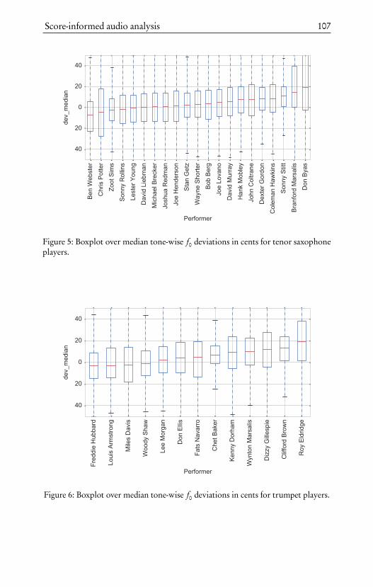
Score-informed audio analysis 107
Ben
Web
ster
Chris P tter
Z t Sims
S n
ny R llins
Lester Y u
ng
David Liebm
an
Micha
el Brecker
J shua
Red
man
J e Hen
ders n
Stan Getz
Wayne
Sh
rter
B b
Berg
J e L
van
David Murray
Han
k M b
ley
J hn
C ltra
ne
Dexter G
rd
n
C lem
an Haw
kins
S n
ny Stitt
Branf rd Marsalis
D n
Byas
Perf rmer
−40
−20
0
20
40de
v_med
ian
Figure 5: Boxplot over median tone-wise f0 deviations in cents for tenor saxophoneplayers.
Fred
die Hub
bard
Louis Arm
stro g
Miles Davis
Woo
dy Sha
w
Lee Morga
Do
Ellis
Fats Navarro
Che
t Baker
Ke
y Dorha
m
Wy to Marsalis
Dizzy Gillespie
Clifford Brow
Roy Eldridge
Performer
−40
−20
0
20
40
dev_med
ia
Figure 6: Boxplot over median tone-wise f0 deviations in cents for trumpet players.
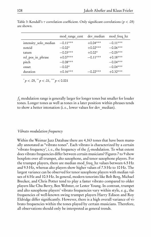
108 Jakob Abeßer and Klaus Frieler
Table 3: Kendall’s τ correlation coefficient. Only significant correlations (p < .05)are shown.
mod_range_cent dev_median mod_freq_hz
intensity_solo_median −0.11*** +0.04*** −0.11***noteid −0.02* +0.02*** −0.06***tatum −0.03*** +0.02* −0.05***rel_pos_in_phrase +0.07*** −0.11*** +0.18***pitch −0.08*** −0.04***onset −0.02* −0.04***duration +0.16*** −0.22*** +0.32***
* p < .05, ** p < .01, *** p < 0.001
f0 modulation range is generally larger for longer tones but smaller for loudertones. Longer tones as well as tones in a later position within phrases tendsto show a better intonation (i. e., lower values for dev_median).
Vibrato modulation frequency
Within the Weimar Jazz Database there are 4,163 tones that have been manu-ally annotated as “vibrato tones”. Each vibrato is characterized by a certain‘vibrato frequency’, i. e., the frequency of the f0-modulation. To what extentdoes vibrato frequencies differ between certain musicians? Figures 7 to 9 showboxplots over all trumpet, alto saxophone, and tenor saxophone players. Forthe trumpet players, there are median mod_freq_hz values between 6.5 Hzand 9.5 Hz, whereas alto players show higher values of 7.5 Hz to 10 Hz. Thelargest variance can be observed for tenor saxophone players with median val-ues of 6 Hz and 10.5 Hz. In general, modern tenorists like Bob Berg, MichaelBrecker, and Chris Potter tend to play a faster vibrato compared to olderplayers like Chu Berry, Ben Webster, or Lester Young. In contrast, trumpetand alto saxophone players’ vibrato frequencies vary within style, e. g., thefrequencies of well-known swing trumpet players Harry Edison and RoyEldridge differ significantly. However, there is a high overall variance of vi-brato frequencies within the tones played by certain musicians. Therefore,all observations should only be interpreted as general trends.

Score-informed audio analysis 109
Harry Edison
Don Ellis
Freddie Hubbard
Woody Shaw
Chet Baker
Miles Davis
Louis Armstrong
Kenny Dorham
Lee Morgan
Wynton Marsalis
Clifford Brown
Roy Eldridge
Performer
2
4
6
8
10
12
14
16mod_freq_hz
Figure 7: Boxplot over vibrato modulation frequency for trumpet players.
Tempo dependency of vibrato modulation frequency
Another interesting question is whether the modulation frequency of vibratotones depends on the tempo of a song. In order to answer this, we detectedthe most prominent modulation frequency fmod between 2 Hz and 15 Hz,as explained in p. 104. We computed the ratio r = Tmod/Tsolo between the‘modulation tempo’, which follows from Tmod = 60 · fmod, and the averagetempo over the solo Tsolo in beats per minute. Figure 10 shows the relationshipbetween r and Tsolo.
As can be observed in Figure 10, there is no evidence in the Weimar JazzDatabase that performers adapt the speed of their vibrato to integer multiplesof the current tempo. For tempos above 150 bpm (medium and fast solos),the modulation frequency varies between the beat level (quarter note) andthe 16th note level. For slower tempos, the vibrato can be up to 10 times fasterthan the beat tempo.
Intensity estimation
Dynamics are essential to any music performance (Fraisse, 1982; Langner& Goebel, 2003). Supposedly, implicit syntactical rules as well as expressiveintentions influence how musicians apply dynamics. Musicians can accentuatecertain parts of musical phrases by playing tones with different intensities,

110 Jakob Abeßer and Klaus Frieler
John
ny Hod
ges
Art Pep
per
Pau
l Desmon
d
Son
ny Stitt
Cha
rlie Parker
Ben
ny Carter
Ornette Colem
an
Lee Kon
itz
Eric Dolph
y
Steve Colem
an
Phil W
oods
Performer
2
4
6
8
10
12
14
16mod
_freq_
hz
Figure 8: Boxplot over vibrato modulation frequency for alto saxophone players.
Chu
Ber
ry
Ben
Web
ster
Zoot
Sim
s
Lest
er Y
oung
Don
Bya
s
Way
ne S
horte
r
Dav
id M
urra
y
Han
k M
oble
y
Son
ny S
titt
Dex
ter G
ordo
n
Bra
nfor
d M
arsa
lis
Josh
ua R
edm
an
Sta
n G
etz
Dav
id L
iebm
an
Joe
Lova
no
Son
ny R
ollin
s
Bob
Ber
g
John
Col
trane
Mic
hael
Bre
cker
Joe
Hen
ders
on
Chr
is P
otte
r
Performer
2
4
6
8
10
12
14
16
mod
_fre
q_hz
Figure 9: Boxplot over vibrato modulation frequency for tenor saxophone players.
i. e., “local stresses” (Lerdahl & Jackendoff, 1983). In regard to meter, theemphasis of certain tones via intensity changes allows musicians both tounderline the given metrical structure and to imply additional rhythms, e. g.,by using syncopation (Pfleiderer, 2006). Two prominent examples are clarinet
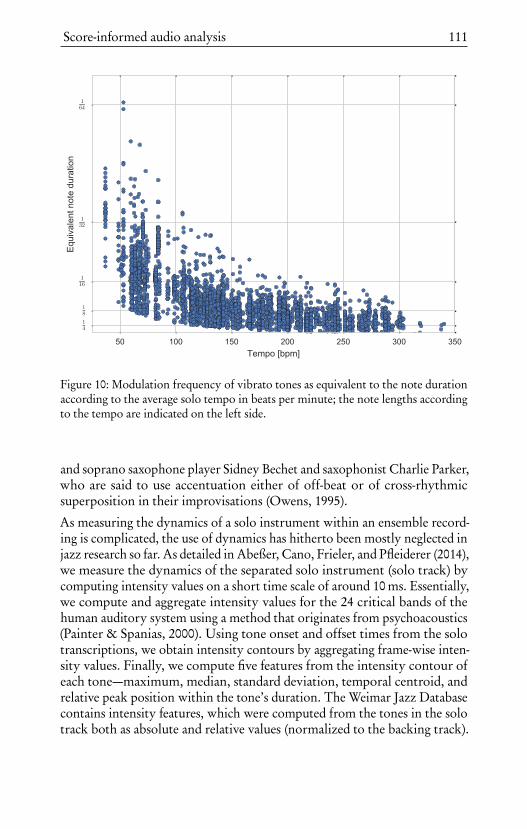
Score-informed audio analysis 111
50 100 150 200 250 300 350Tempo [bpm]
14
18
116
132
164
Equ
ivalen
t note du
ratio
n
Figure 10: Modulation frequency of vibrato tones as equivalent to the note durationaccording to the average solo tempo in beats per minute; the note lengths accordingto the tempo are indicated on the left side.
and soprano saxophone player Sidney Bechet and saxophonist Charlie Parker,who are said to use accentuation either of off-beat or of cross-rhythmicsuperposition in their improvisations (Owens, 1995).
As measuring the dynamics of a solo instrument within an ensemble record-ing is complicated, the use of dynamics has hitherto been mostly neglected injazz research so far. As detailed in Abeßer, Cano, Frieler, and Pfleiderer (2014),we measure the dynamics of the separated solo instrument (solo track) bycomputing intensity values on a short time scale of around 10 ms. Essentially,we compute and aggregate intensity values for the 24 critical bands of thehuman auditory system using a method that originates from psychoacoustics(Painter & Spanias, 2000). Using tone onset and offset times from the solotranscriptions, we obtain intensity contours by aggregating frame-wise inten-sity values. Finally, we compute five features from the intensity contour ofeach tone—maximum, median, standard deviation, temporal centroid, andrelative peak position within the tone’s duration. The Weimar Jazz Databasecontains intensity features, which were computed from the tones in the solotrack both as absolute and relative values (normalized to the backing track).

112 Jakob Abeßer and Klaus Frieler
Table 4: Highest-ranked and lowest-ranked performers sorted in descending orderaccording to Pearson correlation coefficient values between median tone intensityand pitch, note duration, or relative note position within a phrase (averaged over allsolos by a performer); both mean and standard deviation values are given.
# pitch duration rel_pos_in_phrase
1 Don Ellis (tp)(0.55 ± 0.06)
Lionel Hampton (vib)(0.29 ± 0.09)
Branford Marsalis (ts)(-0.09 ± 0.02)
2 Sonny Stitt (as, ts)(0.53 ± 0.18)
Fats Navarro (tp)(0.26 ± 0.04)
John Coltrane (ss, ts)(-0.09 ± 0.02)
3 Chet Baker (tp)(0.52 ± 0.18)
Phil Woods (as)(0.18 ± 0.05)
Stan Getz (ts)(-0.12 ± 0.01)
4 Bix Beiderbecke (cor)(0.50 ± 0.10)
Dizzy Gillespie (tp)(0.15 ± 0.01)
Sonny Stitt (as, ts)(-0.14 ± 0.03)
5 Fats Navarro (tp)(0.48 ± 0.11)
Michael Brecker (ts)(0.12 ± 0.04)
Ben Webster (ts)(-0.15 ± 0.01)
6 Lee Konitz (as)(0.46 ± 0.15)
Cannonball Adderley (as)(0.11 ± 0.01)
Ornette Coleman (as)(-0.16 ± 0.02)
7 Kenny Dorham (tp)(0.45 ± 0.16)
John Coltrane (ss, ts)(0.10 ± 0.12)
Clifford Brown (tp)(-0.16 ± 0.06)
52 Michael Brecker (ts)(0.14 ± 0.02)
David Murray (ts)(-0.23 ± 0.08)
Paul Desmond (as)(-0.28 ± 0.14)
53 Hank Mobley (ts)(0.14 ± 0.01)
Gerry Mulligan (bs)(-0.27 ± 0.11)
David Murray (ts)(-0.29 ± 0.09)
54 Wynton Marsalis (tp)(0.09 ± 0.24)
Paul Desmond (as)(-0.29 ± 0.11)
Lester Young (ts)(-0.29 ± 0.04)
55 Bob Berg (ts)(0.07 ± 0.14)
Don Byas (ts)(-0.30 ± 0.12)
Coleman Hawkins (ts)(-0.30 ± 0.03)
56 Johnny Dodds (cl)(-0.02 ± 0.27)
Louis Armstrong (cor, tp)(-0.34 ± 0.02)
Louis Armstrong (cor, tp)(-0.32 ± 0.10)
57 Joshua Redman (ts)(-0.22 ± 0.02)
Steve Lacy (ss)(-0.34 ± 0.21)
Don Byas (ts)(-0.36 ± 0.04)
58 Chris Potter (ts)(-0.24 ± 0.04)
Bix Beiderbecke (cor)(-0.51 ± 0.17)
Bix Beiderbecke (cor)(-0.41 ± 0.08)
Context-dependency of tone intensities
Are there any correlations between a tone’s intensity and its pitch height,its duration, or its position within a phrase? In order to find an answer tothese issues, we computed the Pearson correlation coefficient between tone-wise median intensity values and the context parameters pitch, duration, andrel_pos_in_phrase as explained in p. 106. In Table 4, the artists in the WeimarJazz Database with the highest and lowest average correlation coefficientsaveraged over the corresponding solos are listed; both the mean and standarddeviation are shown, and only musicians with significant correlations aredisplayed. It is not surprising that most of the solos show a positive correlationbetween intensity and pitch since, in general, higher notes are played moreloudly. Notable exceptions are the two modern tenor saxophone playersJoshua Redman and Chris Potter with negative correlation values of around

Score-informed audio analysis 113
−0.2, presumably due to several loud tones which are ‘honked’ at the verybottom of the tenor saxophone range.
The correlation between tone intensity and duration seems well balancedamong artists and no instrument-specific tendencies towards positive or neg-ative correlation values could be observed. As it becomes obvious from thethird column, tones at the beginning of musical phrases are generally playedmore loudly than tones at the end. This seems to be true in particular forearlier trumpet and cornet players such as Bix Beiderbecke and Louis Arm-strong and tenor saxophone players like Don Byas, Coleman Hawkins, LesterYoung, and David Murray. However, saxophone players such as BranfordMarsalis, John Coltrane, and Stan Getz manage very well to play at the samedynamic level throughout an entire phrase.
Phrase-wise intensity and pitch contours
The movement of pitch and intensity within melodic phrases has a stronginfluence on the overall perception of a melody (Müllensiefen, Wiggins, &Lewis, 2008). In this study, we compare pitch contours and intensity contoursof phrases taken from the solos in the Weimar Jazz Database. We modifiedHuron’s classification of melodic contours of folk songs (Huron, 1996) inorder to make it suitable for the very long phrases which are often encoun-tered in jazz (Abeßer, Frieler, et al., 2017). For both parameters, pitch andintensity, five contour types, ‘horizontal’, ‘ascending’, ‘descending’, ‘convex’,and ‘concave’, are distinguished. We first compute the median intensity valuesv1, v2, and v3 within the first 25 %, the central 50 %, and the final 25 % ofthe phrase duration over tone-wise pitch and intensity values. Based on boththe median intensity and pitch values of all tones in a given phrase, the first25 %, the central 50 %, and the final 25 % of tones are grouped into threesegments. Furthermore, based on the median values vi within the i -th group,the differences between adjacent groups are computed using a tolerance value∆vmin.
Then, we compare the segment intensity difference∆vi via
∆vi =¨
sign(vi+1− vi ), if
vi+1− vi
≥∆vmin,0, otherwise.
using the threshold ∆vmin = 0.1 (maxi vi −mini vi ). Finally, the contourtype is determined using the heuristic given in Table 5, based on the pairsof segment intensity differences (∆v1,∆v2). Phrases with a length of fewerthan 4 tones are grouped into an additional category.

114 Jakob Abeßer and Klaus Frieler
Table 5: Heuristic for the classification of phrase contours. Each phrase contour typeis based on differences ∆v1 and ∆v2 between adjacent segment pairs according toeither pitch or intensity.
Contour Type (∆v1,∆v2)
Horizontal (0,0)Ascending (0,1), (1,0), (1,1)Descending (0,−1), (−1,0), (−1,−1)Concave (−1,1)Convex (1,−1)
Table 6: Percentage of intensity and pitch contour types in jazz solo phrases.
Contour Type Intensity Pitch
< 4 notes 10.1 10.1Horizontal 12.9 3.5Convex 13.4 17.4Concave 9.7 10.9Ascending 13.6 20.0Descending 40.3 38.1
Intensity and pitch contour types in musical phrases
How often do the the pitch and intensity contour types detailed in theprevious section occur within the solos in the Weimar Jazz Database? Arethere any correlations between pitch contours and intensity contours?
As shown in Table 6, descending contours appear most often for both inten-sity and pitch. Ascending and convex pitch contours also appear quite often,while for intensity, almost non-descending contour types appear compara-bly often, except for horizontal contour, i. e., playing at one and the samedynamic level throughout a phrase.
Table 7 illustrates how often different intensity and pitch contours co-occur.All pitch contour types most often coincide with the corresponding intensitycontour (32.9 % on average) or with a descending intensity contour (41.4 %on average). This finding is confirmed by the positive correlation betweenintensity and pitch shown in p. 112.

Score-informed audio analysis 115
Table 7: Percentage of co-occurrence of intensity and pitch contour in jazz solo phrases(minimum length is 4 tones).
Pitch Contour Type Intensity Contour Type
Horiz. Conv. Conc. Ascend. Descend.Horizontal 24.5 7.2 7.8 19.1 41.3Convex 10.6 30.1 7.9 13.7 37.7Concave 16.9 7.4 23.6 11.0 41.2Ascending 14.7 16.3 11.7 28.5 28.8Descending 14.1 10.1 8.3 9.5 57.9
Alternating eighth-note accentuations
It is claimed that many jazz musicians contribute to the swing feeling of theirplaying by accentuating every second eight-note within eight-note chains.The tone-wise intensity values extracted by our score-informed audio analysismethodology allow for an inspection of this hypothesis. For each solo, weperformed a paired t-test between the median tone intensity values of thesecond and first eighths in eight-note sequences. We selected all solos with atleast 10 eight-note pairs, which led to a subset of 77 solos from the WeimarJazz Database.
After selecting solos with significant differences between both eighths ( p <0.05) according to the t-test, we computed Cohen’s d to measure the effectsize (Cohen, 1988). In total, we found 67 solos with positive values for d andonly 10 solos with negative values for d . Therefore, most jazz musicians tendto play the first or on-beat eighth note louder than the second or off-beateighth. In contrast to the hypothesis cited above, there is a clear trend towardson-beat accentuation, at least within the Weimar Jazz Database solos. Theten solos with the highest and lowest effect size values are shown in Table 8.In general, there is a higher effect size for solos with positive d , i. e., withemphasis on the first eighths.
Since the five solos with the highest effect size are played by traditional andswing musicians, there seems to be a tendency to accent the on-beat eighthsby playing them more loudly in older styles. However, modern saxophoneplayers such as David Liebman, Zoot Sims or Joe Henderson follow thistendency, too. It has to be further explored whether intensity differences ofeighth pairs are stylistic traits of individual musicians or depend on otheraspects such as the overall tempo.

116 Jakob Abeßer and Klaus Frieler
Table 8: Ten solos with the highest effect size for both positive intensity differences(first eighths louder than second eighths) and negative intensity differences.
Performer Title Cohen’s d
Bix Beiderbecke (cor) Margie 1.23*
Sidney Bechet (ss) Limehouse Blues 1.04***
Lionel Hampton (vib) High Society 0.90***
Benny Goodman (cl) Tiger Rag 0.89***
Johnny Dodds (cl) Heebie Jeebies 0.87*
David Liebman (ss, ts) Nica’s Dream 0.85**
Zoot Sims (ts) Night and Day 0.83***
Joe Henderson (ts) Totem Pole 0.83*
J.C. Higginbotham (tb) Baby Won’t You PleaseCome Home
0.80**
Coleman Hawkins (ts) It’s Only a Papermoon 0.77**
Stan Getz (ts) Blues in the Closet −0.19**
Herbie Hancock (p) Hand Jive −0.23*
Clifford Brown (tp) I’ll Remember April −0.28*
Chet Baker (tp) You’d Be So Nice toCome Home to
−0.33*
Phil Woods (as) Strollin’ with Pam −0.34**
Kai Winding (tb) Tiny’s Blues −0.36*
Milt Jackson (vib) Don’t Get AroundMuch Anymore
−0.40*
Hank Mobley (ts) Soul Station −0.40*
Fats Navarro (tp) Good Bait −0.52*
Steve Turre (tb) Steve’s Blues −0.58***
* p < .05, ** p < .01, *** p < 0.001
Timbre analysis
Jazz musicians are said to create and develop an individual personal ‘sound’in order to be acknowledged as unique and creative artists (Berliner, 1994;Jackson, 2012) While young musicians learn and grow by imitating oldermusicians, they are generally not appreciated as ‘real’ jazz musicians by theirpeers or by critics and the audience until the have found their own instrumen-tal ‘voice’ with a distinctive ‘sound’. However, what actually contributes to apersonal style or ‘sound’ is not easy to grasp. One might define the ‘sound’ ofa jazz musician as a combination of a characteristic instrumental timbre and

Score-informed audio analysis 117
preferred sound effects (such as growls or slides), dynamics and articulation,as well as structural idiosyncrasies such as the usage of certain rhythmic ormelodic patterns or catch-phrases, or an individual approach to harmony orto solo dramaturgy. While in this usage the term ‘sound’ tends to becomesynonymous with ‘style’, we prefer to focus on aspects of timbre as detectablefrom single tones within a musician’s instrumental improvisations. Couldtimbral characteristics of single tones or a certain amount of tones played by ajazz musician be used to distinguish his ‘sound’ from that of other musicians?And if so: Which sonic features are the decisive factors?
In this section, we aim to distinguish between the ‘sound’ of different jazzmusicians by examining timbral characteristics of their improvisations. Inparticular, we focus on trumpet (tp), alto saxophone (as), and tenor saxophone(ts) musicians with at least four solos included in the Weimar Jazz Database.
Method
We approach the task by first separating the solo instrument from the ensem-ble recording using automatic source separation as explained above (p. 101).Then we extract several acoustic features from the solo instrument track byanalyzing the corresponding magnitude spectrograms of each tone. Thesefeatures quantify spectral and temporal properties such as the tone’s envelopecontour shape and the energy distribution across the tone’s partials. Finally,we apply machine learning algorithms to learn artist-specific timbre patternsfrom a large set of representative solo excerpts taken from the Weimar JazzDatabase.
Based on the STFT magnitude spectrogram M of a tone in the separatedsolo track, we use Non-Negative Matrix Factorization (NMF, D. D. Lee &Seung, 2001) with one component to represent each tone as a product of aspectral envelope S and a temporal envelope A. An example of such a simpledecomposition is shown in Figure 11. In the temporal envelope A, the shortattack part as well as the decay and release parts of the tone’s envelope arevisible. The peaks in the spectral envelope S indicate the partials (overtones)of the tone. Also, it becomes apparent that higher partials show higher energythan lower partials.
Since the temporal envelope, in particular the attack part with its risingamplitude shape, is important for the human recognition of instrumenttimbres, we compute two additional representations. We calculated the firstderivative∆A of the temporal envelope A as a second representation and thehistogram values N∆A over ∆A with 10 equally spaced histogram bins as athird representation.

118 Jakob Abeßer and Klaus Frieler
Figure 11: Decomposition of a tone’s magnitude spectrogram M into a spectral enve-lope S and a temporal envelope A.
Based on these two representations S and A, we extracted 127 audio featureswhich combine state-of-the-art features from the field of MIR with severalnovel contributions. The main categories of these features are listed in Table 9.The first group of features based on the spectral envelope S includes standardlow-level features such as the statistical measures spectral centroid, spread,skewness, and kurtosis as well as spectral shape characteristics such as spectraldecrease, slope, flatness, and roll-off frequency. Most of these features imple-ment summative statistical measures while some of them capture higher-levelproperties such as the energy distribution over partials (relative harmonicmagnitudes, odd-to-even ratio, tristimulus 1-3) or the tone envelope shape(log attack time, log decay time, multi-resolution gamma filter bank) (Peeters,2004).
Mel-Frequency Cepstral Coefficient (MFCC) features originate from speechprocessing and give a compact description of the spectral envelope shape.We use the MFCC coefficients 2 to 13. The Octave-Based Spectral Contrast(OSC) features characterize spectral peaks and valleys in different octave-related frequency bands, which can indicate the presence of harmonic peaks(overtones) and noise-like components in an audio signal (C.-H. Lee, Shih,Yu, & Lin, 2009).

Score-informed audio analysis 119
Table 9: Spectral and temporal features to characterize the timbre of tones in a jazzsolo.
Category Feature
Spectral features Statistics (centroid, spread, skewness, kurtosis), shape(decrease, slope, flatness, roll-off), Mel-Frequency Cep-stral Coefficients (MFCC), spectral contrast (octave-based, shape-based), inharmonicity coefficient, relativepartial magnitudes, odd-to-even ratio, tristimulus 1-3
Temporal features Statistics (centroid, spread, skewness, kurtosis), shape(decrease, slope, flatness, roll-off), relative attackpart length, log attack time, log decay time, Multi-Resolution Gamma Filter Bank (MRGF)
Furthermore, features to quantify the relationships between partial frequen-cies and between partial magnitudes are computed. Therefore, we first esti-mate the fundamental frequency of a given tone as the frequency position thatcorresponds to the highest cross-correlation between the spectral envelope Sand an idealized harmonic spectrogram with unit peaks at the harmonic fre-quency positions (Abeßer & Schuller, 2017). The ‘inharmonicity coefficient’measures how strong the partial frequencies deviate from integer multiplesof the fundamental frequency. We estimate the coefficient from the spectralenvelope S as proposed in (Abeßer & Schuller, 2017). By normalizing thepartial magnitudes in S to the magnitude of the fundamental frequency, wecompute the ‘relative partial magnitudes’. As proposed by Peeters (Peeters,2004), we additionally compute the ‘odd-to-even ratio’ and the three ‘tristim-ulus’ features, which provide alternative relationship measures between thepartial magnitudes to describe the timbre of a given tone.
The second set of features includes temporal features. Similarly to the spectralaudio features, we compute the aforementioned low-level statistic descriptorson the three temporal representations A,∆A, and N∆A to characterize theirgeneral distribution. Based on the position of the global peak in A, we segmentthe temporal envelope into an attack part and a decay part. From the durationsof the two parts, we compute the ‘relative attack part length’ (by normalizingto the overall tone duration) and the log attack and decay time. In addition,we compute the ‘Multiresolution Gamma Filterbank Response’ (MGFR)features (Tjao & Liu, 2010). The applied filter bank consists of 32 gamma filterkernels that resemble different temporal envelope shapes with varying attacktimes and overall durations. The proposed set of 127 features is computed forall tones in a given solo.

120 Jakob Abeßer and Klaus Frieler
Table 10: Data set for automatic performer identification for trumpet (tp), alto saxo-phone (as), and tenor saxophone (ts) players.
Instrument Performer
tp (13) Chet Baker, Clifford Brown, Dizzy Gillespie, Don Ellis, FatsNavarro, Freddie Hubbard, Kenny Dorham, Lee Morgan,Louis Armstrong, Miles Davis, Roy Eldridge, Woody Shaw,Wynton Marsalis
as (11) Art Pepper, Benny Carter, Cannonball Adderley, CharlieParker, Eric Dolphy, Lee Konitz, Ornette Coleman, PaulDesmond, Phil Woods, Sonny Stitt, Steve Coleman
ts (21) Ben Webster, Bob Berg, Branford Marsalis, Chris Potter,Coleman Hawkins, David Liebman, David Murray, DexterGordon, Don Byas, Hank Mobley, Joe Henderson, Joe Lo-vano, John Coltrane, Joshua Redman, Lester Young, MichaelBrecker, Sonny Rollins, Sonny Stitt, Stan Getz, WayneShorter, Zoot Sims
Timbre-based performer classification
To what extent can a soloist be identified among his instrument peers basedon the tone-wise features specified above (cf. p. 116)? In the following, wefocus on all trumpet, alto saxophone, and tenor saxophone players includedin the Weimar Jazz Database with at least four solos as listed in Table 10. Foreach solo, we extracted features from the first 100 tones with a duration ofmore than 100 ms.
The classification was performed using leave-one-label-out cross-validation.Here, the total data set of tones is repeatedly split into a training set, which isused to train the classification model, and a test set, which is used to evaluatethe model’s performance. The leave-one-label-out strategy implies that in eachcross-validation fold, tones from all solos of a given artist except one solo areused to train the classification algorithm while the tones from the remainingsolo are used as a test set. This strategy reflects the use case, in which a trainedsystem is used to classify an artist with tones taken from a previously unseensolo. The final model performance is computed by averaging the performancemeasures in each cross-validation fold.
In each fold, we first standardize the features to zero mean and unit varianceand then apply Linear Discriminant Analysis (LDA) to transform the initialfeature space. LDA maximizes the variance between tones of different per-formers and minimizes the variance between tones of the same performer in
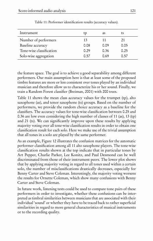
Score-informed audio analysis 121
Table 11: Performer identification results (accuracy values).
Instrument tp as ts
Number of performers 13 11 21Baseline accuracy 0.08 0.09 0.05Tone-wise classification 0.29 0.36 0.25Solo-wise aggregation 0.57 0.69 0.57
the feature space. The goal is to achieve a good separability among differentperformers. Our main assumption here is that at least some of the proposedtimbre features are more or less consistent over tones played by an individualmusician and therefore allow us to characterize his or her sound. Finally, wetrain a Random Forest classifier (Breiman, 2001) with 200 trees.
Table 11 shows the mean class accuracy values for the trumpet (tp), altosaxophone (as), and tenor saxophone (ts) groups. Based on the number ofperformers, we provide the random choice accuracy as a baseline for theclassifiers. The accuracy values for tone-wise classification between 0.25 and0.36 are low even considering the high number of classes of 11 (as), 13 (tp)and 21 (ts). We can significantly improve upon these results by applyingmajority voting over all tone-wise classification results in order to obtain oneclassification result for each solo. Here we make use of the trivial assumptionthat all tones in a solo are played by the same performer.
As an example, Figure 12 illustrates the confusion matrices for the automaticperformer classification among all 11 alto saxophone players. The tone-wiseclassification results shown at the top indicate that in particular tones byArt Pepper, Charlie Parker, Lee Konitz, and Paul Desmond can be welldiscriminated from those of their instrument peers. The lower plot showsthat by applying majority voting in regard to all tones used within a certainsolo, the number of misclassifications drastically decreases, especially forBenny Carter and Steve Coleman. Interestingly, the majority voting worsensthe results for Ornette Coleman, which show many confusions with BennyCarter and Steve Coleman.
In future work, listening tests could be used to compare tone pairs of theseperformers in order to investigate, whether these confusions can be inter-preted as timbral similarities between musicians that are associated with theirindividual ‘sound’ or whether they have to be traced back to rather superficialsimilarities in regard to more general characteristics of musical instrumentsor to the recording quality.

122 Jakob Abeßer and Klaus Frieler
(a) Tone-wise classification.
(b) Solo-wise classification using majority voting.
Figure 12: Confusion matrices for performer identification (alto saxophone players).

Score-informed audio analysis 123
With our approach, known sonic similarities between jazz musicians canbe systematically verified and formerly unknown sonic similarities betweenmusicians might be uncovered. Moreover, an automatic analysis of largearchives of jazz recordings would permit an investigation of how the timbralcharacteristics of the most common jazz instruments have changed over thecourse of jazz history. Using an algorithmic procedure of timbre characteri-zation could also help to clean up metadata annotations in jazz archives andto enrich algorithms for automatic performer identification in jazz ensemblerecordings.
Walking bass transcription
Method
Walking bass lines are a significant and even defining feature of many jazzstyles. They mostly consist of quarter-note chains to support the main met-rical structure and to provide harmonic orientation by emphasizing chordtones such as roots, thirds, and fifths. In a recent study (Abeßer, Balke, Frieler,Pfleiderer, & Müller, 2017), we proposed a novel method to automaticallytranscribe the walking bass line from jazz recordings. The central idea is totrain a deep neural network to learn a mapping from a mixture (constant Q)spectrogram to a bass saliency representation. This representation measuresthe likelihood of the bass line playing certain pitches at a certain time. Themapping is learned automatically based on labeled training data, i. e., 31 jazzrecordings selected from the Weimar Jazz Database with manually createdbass line transcriptions.
Based on the bass saliency representation, we avoid the error-prone step ofautomatic tone formation, i. e., grouping salient pitches to tone events, butinstead use manual beat annotations from the Weimar Jazz Database andestimate the most salient bass pitches for each beat. Based on a separatedtest set of ten bass lines, the proposed approach achieved a beat-wise pitchaccuracy of 83 % and outperformed three state-of-the-art bass transcriptionalgorithms for the given task.
Walking bass analysis
To demonstrate the analytical potential of our method for walking basstranscription, we will present some first exploratory studies of walking basspitches, mostly with respect to the underlying harmony. It is the usual taskof the bass player to convey the chords of a tune while also creating smooth

124 Jakob Abeßer and Klaus Frieler
and interesting lines. The golden rule (in common practice jazz, at least)is to play the root of the chord on the first beat of a bar. Doing so clearlypresents harmonic guidance for the other players and leaves also the piano (orother chord) player the freedom to omit the root and to play more modernsounding voicings, often using harmonic extensions (e. g., [9, ]11, [13). Besidesthe root, the fifth, the third and, to some extent, the seventh are the nextmost important tones for conveying a chord. However, focusing exclusivelyon chord tones would create arpeggios with rather large intervals in between,which neither form smooth lines nor are they generally easy to play on adouble bass. Hence, besides the ‘root-on-the-first-beat rule’, bass players havesome freedom (or are even supposed) to create well-sounding lines. Quiteprobably, they rely here on a large repertoire of patterns, particularly forfrequently occurring accord transitions, e. g., II-V combinations in the morecommon keys such as F, B[, and C. An in-depth analysis of walking basspatterns cannot be carried out here, but by using simple distributions of pitchclasses some insights into the principles of creating walking bass lines canalready be gained. We used 422 walking bass lines with annotated rhythmfeel ‘swing’ extracted from the solos of the Weimar Jazz Database using themethod described above. This resulted in 110,703 bass tones for which contextinformation was also gathered, most importantly the annotated chords.
First, it might be interesting to look at the distribution of pitch classes15). InTable 12, the distribution of pitch classes across all solos is shown. Interest-ingly, this distribution does not so much reflect the most common keys, as itdoes the specifics of the double bass. The pitch classes which are available asopen strings, i. e., E, A, D, and G, are the most frequent, with G being themost frequent of all, which might be explained by the fact that the pitch G isa more frequent chord root in the most common keys than the other threepitches E, A, and D. Besides these four most frequent ones, the other pitchclasses are basically uniformly distributed.
Secondly, we take a look at the distribution of chordal pitch classes, i. e., thepitch class of each bass tone in relation to the root of the chord. Since majorand minor chords have different thirds, we also annotated each chord with itsbasic triad type (major or minor) to see whether the thirds are used differently.In Figure 13, boxplots for chordal pitch classes differentiated with respect tobasic triad types are shown. One clearly sees that the root of the chord (cpc= 0) is by far the most frequent chord pitch class (about 30 % on average forboth minor and major), followed by the fifth (cpc = 7), with about 10 %. Inboth major and minor contexts, the next most common chordal pitch class
15We restrict ourselves to pitch classes here to circumvent problems with octave errors intro-duced by the extraction algorithm.
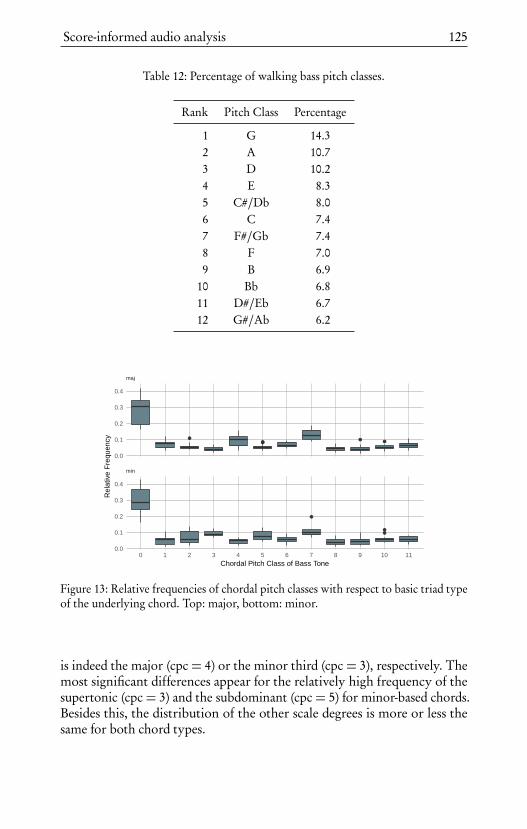
Score-informed audio analysis 125
Table 12: Percentage of walking bass pitch classes.
Rank Pitch Class Percentage
1 G 14.32 A 10.73 D 10.24 E 8.35 C#/Db 8.06 C 7.47 F#/Gb 7.48 F 7.09 B 6.9
10 Bb 6.811 D#/Eb 6.712 G#/Ab 6.2
min
maj
0 1 2 3 4 5 6 7 8 9 10 11
0.0
0.1
0.2
0.3
0.4
0.0
0.1
0.2
0.3
0.4
Chordal Pitch Class of Bass Tone
Rel
ativ
e F
requ
ency
Figure 13: Relative frequencies of chordal pitch classes with respect to basic triad typeof the underlying chord. Top: major, bottom: minor.
is indeed the major (cpc = 4) or the minor third (cpc = 3), respectively. Themost significant differences appear for the relatively high frequency of thesupertonic (cpc = 3) and the subdominant (cpc = 5) for minor-based chords.Besides this, the distribution of the other scale degrees is more or less thesame for both chord types.

126 Jakob Abeßer and Klaus Frieler
3 4
1 2
0 1 2 3 4 5 6 7 8 9 10 11 0 1 2 3 4 5 6 7 8 9 10 11
0%
10%
20%
30%
40%
50%
0%
10%
20%
30%
40%
50%
Chordal Pitch Class of Bass Tone
Per
cent
age
(%)
Figure 14: Relative frequencies of chordal pitch classes with respect to beat position.
Since all selected solos are in common 44 time, we can easily differentiate
the distribution of chordal pitch classes with respect to beat positions asseen in Figure 14. The root is still the most common chordal pitch classfor all four positions, but, as expected, even more so for the first beat withmore than 40 %, which is, however, at the same time rather unexpectedlylow. Interestingly, no clear pattern for the other chordal pitch classes can beidentified, which hints at a rather large variation and fluidity of walking basslines.
Thirdly, one could conjecture that differences in chordal pitch class usagemight exist with respect to commonness of chords. To examine this point,we calculated chordal pitch class frequencies with respect to the frequency ofthe root of the underlying chord, again differentiated for major and minorbasic triad types (Figures 15 and 16, for the relative frequencies of chord rootpitch classes see Table 13). Pearson’s correlations can be found in Table 14.Clear trends can be seen for both triad types. For instance, the chord rootpitch class occurs less often for more common chord roots in both cases, verystrongly so for major chords (rma j =−.92), slightly less so for minor chords(rmi n =−.64). The second scale degree (cpc = 2) increases in frequency formore common chords, particularly for minor chords (rma j = .63, rmi n = .85).Interestingly, the frequency of major thirds (cpc = 4) increases for morecommon chord roots as well as for minor chords (rma j = .86, rmi n = .8),but the frequency of minor thirds (cpc = 3) decreases for minor chords. Theincrease in major thirds could be partly explained by their use as chromaticpassing tones to the root of a following dominant seventh chord, since minorchords very often occur in ii7-V combinations. An examination of beat

Score-informed audio analysis 127
Table 13: Relative frequencies of chord root pitch classes for major and minor triadtype chords.
Major MinorRank Root PC Rel. Frequency Root PC Rel. Frequency
Major All Minor All
1 F 0.18 0.12 C 0.20 0.062 Bb 0.17 0.12 G 0.17 0.053 Eb 0.15 0.10 F 0.15 0.054 C 0.12 0.08 D 0.14 0.045 G 0.10 0.07 A 0.07 0.026 Ab 0.08 0.06 Bb 0.07 0.027 D 0.07 0.05 Eb 0.06 0.028 Db 0.05 0.03 E 0.04 0.019 A 0.02 0.02 Gb 0.04 0.0110 B 0.02 0.01 B 0.02 0.0111 Gb 0.02 0.01 Db 0.02 0.0112 E 0.02 0.01 Ab 0.02 0.01
Note. Chord root frequencies are counted beat-wise.
positions of major thirds over minor seventh chords shows that they occurmore often on weak beats 2 and 4 (54 % vs. 46 % for beat 1 and 3). Thefrequency of fifths (cpc = 7) decreases for less common chord roots in thecase of major chords (rma j =−.41), but not significantly so, and increases forminor chords (rmi n = .68). Finally, the frequency of major sixths (cpc = 10)and minor sevenths (cpc = 11) are higher for major chords with increasingcommonness of the chord roots (rma j = .81 and rmi n = .66).
How to interpret these interesting trends? The increased use of roots with lesscommon chords might indicate a “safe playing” strategy, since there might befewer preconceived patterns at hand, so bass players tend to rely on the easiestand safest solution, the root. On the other hand, the more common a chord(root), the more freedom and the more patterns the bass player might have attheir disposal due to their playing and practice routines. Complementarily,one might conjecture that the more common chords tend to occur in longerstretches, i. e., as a tonic or subdominant chord in a standard 12-bar blues(e. g., F or B[ blues) where chords can last up to four bars and more in arow. This leaves room for the bass player to create longer, more diverse,and interesting lines, possibly also including spontaneous, temporary, and

128 Jakob Abeßer and Klaus Frieler
8 (n.s.) 9 (**) 10 (n.s.) 11 (*)
4 (***) 5 (n.s.) 6 (n.s.) 7 (n.s.)
0 (***) 1 (n.s.) 2 (*) 3 (n.s.)
0.0625 0.12500.1250 0.0625 0.12500.1250 0.0625 0.12500.1250 0.0625 0.12500.1250
0.0625 0.12500.1250 0.0625 0.12500.1250 0.0625 0.12500.1250 0.0625 0.12500.1250
0.0625 0.12500.1250 0.0625 0.12500.1250 0.0625 0.12500.1250 0.0625 0.12500.12500.020.030.040.050.060.07
0.1000.1250.1500.175
0.040.060.080.10
0.050.070.090.11
0.050.060.070.080.09
0.04
0.06
0.08
0.0500.0750.100
0.030.040.050.060.070.08
0.025
0.050
0.075
0.100
0.150.200.250.300.350.40
0.04
0.08
0.12
0.16
0.02
0.04
0.06
0.08
Relative Frequency of Root
Rel
ativ
e F
requ
ency
Chord type: maj
Figure 15: Relative frequencies of chordal pitch classes plotted against relative frequen-cies of chord roots for major-based chords. Each panel shows the relative frequencyof the corresponding chordal pitch class on the y-axis for all 12 chord root pitchclasses with the relative frequency on the x-axis. Asterisks in parentheses indicatethe significance of the trend (n.s. = not significant, * = p < .05, ** = p < .01,*** = p < .001).
8 (n.s.) 9 (n.s.) 10 (n.s.) 11 (n.s.)
4 (**) 5 (n.s.) 6 (n.s.) 7 (*)
0 (*) 1 (n.s.) 2 (***) 3 (*)
0.02 0.04 0.06 0.02 0.04 0.06 0.02 0.04 0.06 0.02 0.04 0.06
0.02 0.04 0.06 0.02 0.04 0.06 0.02 0.04 0.06 0.02 0.04 0.06
0.02 0.04 0.06 0.02 0.04 0.06 0.02 0.04 0.06 0.02 0.04 0.06
0.08
0.10
0.12
0.10
0.15
0.20
0.04
0.06
0.08
0.05
0.10
0.020.040.060.08
0.040.060.080.10
0.03
0.06
0.09
0.040.060.080.100.12
0.020.040.060.080.10
0.200.250.300.350.40
0.020.030.040.050.06
0.020.040.060.08
Relative Frequency of Root
Rel
ativ
e F
requ
ency
Chord type: min
Figure 16: Relative frequencies of chordal pitch classes plotted against relative frequen-cies of chord roots for minor-based chords. Each panel shows the relative frequencyof the corresponding chordal pitch class on the y-axis for all 12 chord root pitchclasses with the relative frequency on the x-axis. Asterisks in parentheses indicatethe significance of the trend (n.s. = not significant, * = p < .05, ** = p < .01,*** = p < .001).
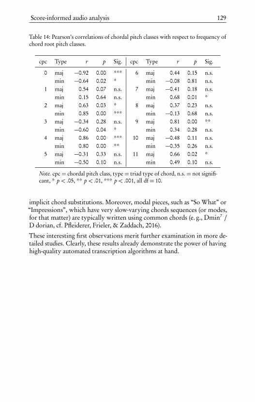
Score-informed audio analysis 129
Table 14: Pearson’s correlations of chordal pitch classes with respect to frequency ofchord root pitch classes.
cpc Type r p Sig. cpc Type r p Sig.
0 maj −0.92 0.00 *** 6 maj 0.44 0.15 n.s.min −0.64 0.02 * min −0.08 0.81 n.s.
1 maj 0.54 0.07 n.s. 7 maj −0.41 0.18 n.s.min 0.15 0.64 n.s. min 0.68 0.01 *
2 maj 0.63 0.03 * 8 maj 0.37 0.23 n.s.min 0.85 0.00 *** min −0.13 0.68 n.s.
3 maj −0.34 0.28 n.s. 9 maj 0.81 0.00 **min −0.60 0.04 * min 0.34 0.28 n.s.
4 maj 0.86 0.00 *** 10 maj −0.48 0.11 n.s.min 0.80 0.00 ** min −0.35 0.26 n.s.
5 maj −0.31 0.33 n.s. 11 maj 0.66 0.02 *min −0.50 0.10 n.s. min 0.49 0.10 n.s.
Note. cpc = chordal pitch class, type = triad type of chord, n.s. = not signifi-cant, * p < .05, ** p < .01, *** p < .001, all df= 10.
implicit chord substitutions. Moreover, modal pieces, such as “So What” or“Impressions”, which have very slow-varying chords sequences (or modes,for that matter) are typically written using common chords (e. g., Dmin7 /D dorian, cf. Pfleiderer, Frieler, & Zaddach, 2016).
These interesting first observations merit further examination in more de-tailed studies. Clearly, these results already demonstrate the power of havinghigh-quality automated transcription algorithms at hand.


Solos: Case studies


Don Byas’s “Body and Soul”
Martin Pfleiderer
Coleman Hawkins’s solo on “Body and Soul” is generally viewed as a mile-stone in the history of jazz improvisation (see, e. g., Schuller, 1989, pp. 441-445; Porter et al., 1993, pp. 173-175; DeVeaux, 1997, pp. 98-110). ColemanHawkins recorded “Body and Soul” in October 1939 and the recording un-expectedly sold over 100 000 copies in the first six months after its release(DeVeaux, 1997, p. 99). In these times, this was a remarkable success for ajazz recording with no singer and no big band—all the more so as Hawkinsdoes not play the melody but just improvises two choruses, accompaniedby a rhythm section and, during the second chorus, by some horn chords.With “Body and Soul”, Hawkins proved that improvisation is the centralartistic achievement of jazz—given that sound recordings could transformelusive improvisations into a lasting art form (cf. DeVeaux, 1997, p. 11). Withthis recording, the “father of the jazz tenor saxophone” (Porter et al., 1993,p. 62) influenced subsequent musicians in their focus on improvisation and,in particular, tenor saxophonists in their improvisations over “Body andSoul” (cf. Bowen, 2011, pp. 23ff.; Pfleiderer, 2011). This chapter is dedicatedto one of those follow-up improvisations over “Body and Soul” recorded inJanuary 1947 by the tenor saxophonist Don Byas and to a comparison withHawkins’s seminal improvisation.
Don Byas—a side figure in jazz history
Today, Don Byas is far less well-known than Hawkins, but nevertheless awidely acknowledged master of the jazz tenor saxophone. He was born in1912 as Carlos Wesley in Muskogee, a little town in Oklahoma, and startedplaying in local swing bands at the age of 17. During his college years (1931–32, at Langston College, Oklahoma), he led a band called Don Carlos and

134 Martin Pfleiderer
His Collegiate Ramblers. After a four-year stay in Los Angeles, Byas movedto New York in 1937 where he started to work with several swing bands, e. g.,those of Don Redman, Lucky Millinder, Andy Kirk, Edgar Hayes, and BennyCarter, and recorded with Billie Holiday. In early 1941, Byas was chosen byCount Basie to be Lester Young’s successor in his big band; he recorded withBasie’s big band and small groups, and started to play at clubs on 52nd Street.Moreover, Byas recorded with Coleman Hawkins, Charlie Parker, and DizzyGillespie as well as for several Hollywood films. Like Coleman Hawkins,Don Byas participated in bebop jam sessions right from its beginnings in theearly 1940s. In 1941, a jam session at Minton’s Playhouse was recorded byJerry Newman, featuring Byas with the Minton’s ‘house band’, including JoeGuy on trumpet, Thelonious Monk on piano, and Kenny Clarke on drums.They played, among other songs, “Body and Soul”; later, parts of the sessionwere issued on a vinyl album called Midnight at Minton’s under the name ofDon Byas. In February 1944, Don Byas participated in one of the first bebopstudio recordings which was made with a twelve-man group led by ColemanHawkins including, among others, bebop pioneers Dizzy Gillespie, OscarPettiford, and Max Roach.
In September 1946, Don Byas went to Europe—following the example ofHawkins, who lived in Europe from 1934 until 1939. At first, Byas touredwith Don Redman’s big band in Denmark, Belgium, Switzerland, and Ger-many. Then, he settled in France and in the early 1950s moved to the Nether-lands where he lived until his death in 1972. During his residence in Europe,Byas had only loose connections to the US jazz scene. Although he playedand sometimes recorded with US jazz musicians such as Dizzy Gillespie,Mary Lou Williams, Bud Powell, or Ben Webster, Byas mostly worked andrecorded with European musicians.
Presumably, his absence from the United States is the main reason why Byasis a rather underrated figure in jazz history. Nevertheless, he has been highlypraised by musicians and connoisseurs. As an example, saxophonist andcomposer Leo T. Sullivan writes on an internet website dedicated to DonByas:
Byas was a masterful swing player with his own style, an ad-vanced sense of harmony, and a confidence that was unmistak-ably his own, immediately recognizable. His sense of dramacoupled with a brilliant use of dynamics and timbre, a deeply-feltromanticism—accomplished both the tenderest warmth and themost strident sting. He never picked up the rhythmic phrases,the lightning triplets, that are indigenous to bop. Yet Charlie

Don Byas’s “Body and Soul” 135
Parker said of him that Byas was playing everything there wasto play.
One of the greatest of all tenor players, Don Byas’ decision tomove permanently to Europe in 1946 resulted in him beingvastly underrated in jazz history books. His knowledge of chordsrivaled Coleman Hawkins, and, due to their similarity in tones,Byas can be considered an extension of the elder tenor. (Sullivan,n.d.)
Despite such enthusiastic assessments, there is almost no analytical researchon Byas’s style of improvisation. For example, Thomas Owens’s stylisticaccount of countless modern jazz musicians dedicates only one paragraph toByas, focusing on his relation to bebop playing (Owens, 1995, p. 72).
In January 1947, one year after his arrival in France, Byas recorded “Body andSoul” with Billy Taylor, piano, Jean Bouchety, double bass, and Buford Oliver,drums. The following analytical case study is an attempt to appreciate severalcharacteristics of this improvisation. First, several techniques of improvisa-tion will be exemplified by analyzing parts of the solo. Then, a comparisonbetween the solos of Byas and Hawkins will investigate commonalities anddifferences between their styles of improvisation.
Don Byas’s “Body and Soul” (1947)
The formal structure of Byas’s “Body and Soul” is clearly modeled afterHawkins’s 1939 version. The recording starts with a four-measure introduc-tion, passes through two improvised choruses, and ends with a rubato cadenza.In contrast to Hawkins, however, Byas returns to paraphrasing the melodyin the last A section of the second chorus. When listening to Don Byas im-provising two choruses on “Body and Soul”, I am in particular impressedby both his warm and intimate tenor sound and his elegant and highly orna-mented melodic lines. His articulation of each tone of these lines is pin-sharp,like a pearl on a string, and he plays with an amazing rhythmic variability,including several moments of brief hesitation and laid back phrases. Afterparaphrasing and commenting on the original melody in the first A section,he departs from the melodic template with sophisticated lines, which flowup and down the whole range of the tenor saxophone. Additionally, thereare clear melodic statements that are accentuated both by sequencing certainmotifs as well as by retarding certain tones and playing them louder at thesame time. One climax of the solo, at least in regard to instrumental virtuos-ity, consists of several lines shortly after the beginning of the second chorus

136 Martin Pfleiderer
(mm. 38–40), which flow up and down with both astonishing velocity andprecise articulation. Another climax is in the last B section (mm. 52 and 53),where Byas jumps two times to the top of the saxophone range, first to D5and then to G5.
In the following, I will give examples for several creative strategies employedin Byas’s solo. The music examples are based on the transcription included inthe Weimar Jazz Database. The score has been re-worked in several respects inorder to make it easier to read. In regard to rhythm, the original transcriptionstrictly follows the position of the tones in relation to a constantly tappedmetric framework. Since Byas tends to play some tones or whole phrasesdeliberately behind the beat, however, there are many odd note values andnote shifts with many slurs over metric positions. In most of the musicexamples below I prefer a simplified and more readable notation where theserhythmic shifts are marked by ‘laid back’ above certain notes and phrases.Moreover, several rests which were omitted by the conversion algorithm areadded as well as a few tones which seemingly went unnoticed by the humantranscriber. Some accidentals are adjusted to the harmonic framework. Therubato cadenza at the end is ignored both for transcription and analysis. Sinceit is not known which chords Byas actually had in mind while improvising hisversion of “Body and Soul”, the annotated chords follow a more sophisticatedjazz re-harmonization of “Body and Soul” in the key of D[ major, whichis included in the Weimar Jazz Database transcription too, rather than thesimple chord progressions in C as originally composed by Johnny Green(Krieger, 1995, pp. 20f.).
Melodic strategies for improvisation
Following proposals by André Hodeir and Gunther Schuller, jazz scholarBarry Kernfeld categorizes three types of jazz improvisation which mayoccur within a certain solo (Kernfeld, 1995, pp. 119-158). While in paraphraseimprovisation there is a close reference to the original melody of a piece, inso-called chorus phrase or formulaic improvisation musicians invent newlines that fit to the harmonies of the original composition. Often, this strategyrelies on a vocabulary of melodic building blocks, patterns or formulas. Inmotivic improvisation, the musicians vary one or several motifs, sometimestaken from the theme of a piece but more often drawn from the ongoingstream of improvisational ideas. All three strategies for improvisation can befound in Byas’s solo on “Body and Soul”.
Byas starts and ends his solo with a paraphrasing of the original melody (firstA section and last A section). An immediate comparison with the original

Don Byas’s “Body and Soul” 137
Figure 1: Original melody of “Body and Soul” (in Db major) and Byas’s improvisationin the first and last A section.
melody (see Figure 1) reveals many of Byas’s techniques of paraphrasing,ornamenting and varying the melody as well as some general features of hisstyle of improvising. In a few cases, he keeps playing the longer and metricallyimportant tones of the original melody, e. g., the F at beat one of m. 6 (bothsections), but more often he does not place the melody tone but a tone fromthe underlying chord on beat one, e. g., at mm. 3 and 5 (both sections), andthen plays the melody a bit later and in a varied and rhythmically condensedmanner, such as in mm. 1, 3, 4, and 5. In between the individual parts of thismelodic skeleton, he often adds ornamenting phrases within the second halfof a measure, such as in mm. 2, 6, and 8 of the first section or mm. 2, 3, 5,and 6 of the last section. As another strategy of ornamentation he plays short

138 Martin Pfleiderer
Figure 2: Don Byas “Body and Soul”, second A section.
figurations before a goal tone, e. g., E and F (end of m. 4) before E[ (m. 5)or D[ and E[ (end of m. 5) before F (m. 6) in the first section. Several timesByas emphasizes certain tones by retarding them. Interestingly, all the clearlylaid back tones in the first section A (see mm. 3, 4 and 7) also stand out asthe highest tones within the melodic contour. In m. 7, he repeats a four-tonemotif one semitone lower. This technique of sequencing is employed by Byasregularly throughout the solo and contributes to the motivic coherence ofhis improvisation.
In the second A section (see Figure 2), Byas departs from paraphrasing theoriginal melody by playing the ascending E[ minor scale. Now, a chorusphrase improvisation in the sense of Kernfeld starts. Byas switches from thepulse in the first eight measures, which is mainly based on eighth triplets,to a sixteenth note pulse. However, he continues to employ strategies offiguration (see, e. g., B and A at the end of m. 9 leading to B[ in m. 10) and ofsequencing by repeating motivic cells a semitone lower, e. g., in m. 12, wherea line upwards is twice followed by a jump down (the third time in m. 13by a line down). In m. 15, he repeats a four-tone figure, with a jump up asixth, a semitone lower. Therefore, chorus phrase improvisation is closelyintertwined with motivic improvisation.

Don Byas’s “Body and Soul” 139
Another strategy of Byas to generate melodic coherence seems to be the usageof an open system of melodic patterns. His pattern vocabulary encompassesboth melodic lines which have a certain salience and recognition value andmore amorphous melodic building blocks that mostly pass unnoticed forthe listener. MeloSpyGUI offers a comfortable functionality to search forvarious kinds of these building blocks or patterns. In general, patterns aredefined as certain sequences of elements (pitches, intervals, etc.) which arerepeated at least a second time within one solo or within a set of severalsolos. Although these patterns are often part of longer lines, their double ormultiple occurrences indicate that they are characteristic for a solo—or, ifoccurring in other solos too, for Byas’s overall personal melodic vocabulary.
Within his improvisation on “Body and Soul”, Byas repeats several long pitchpatterns (see Figure 3). The longest pattern is part of the paraphrasing inthe first A section, containing twelve tones played in m. 6 and then repeatedin the last section over the same chord in mm. 61 and 62 (Figure 3a). Bothmelodies start on beat one with an ascending E[ minor seventh arpeggioand sound similar despite their slightly different rhythms. The second longpattern, consisting of ten tones, is played in m. 26 and repeated closely inm. 29 (Figure 3b). Both patterns start on different metric points and are partof longer lines, which continue differently.
Furthermore, there are three pitch patterns containing seven tones (e. g., inmm. 30 and 62, see Figure 3c), five patterns with six tones, and twelve patternswith five tones. While most of the patterns occur only two times, two of thefive-tone patterns appear three times at different positions within the solo.The coverage with patterns of five or more tones within the whole solo isalmost 27.6 % (disregarding overlapping patterns). If one looks at patterns offour or more pitches, the percentage rises to more than 50 % and to about80 % if one disregards absolute pitch and instead allows for patterns of threeidentical intervals. Of course, these patterns encompass chord arpeggios andsimple scale sections, too. Nevertheless, the repeated use of such buildingblocks may contribute to an overall impression of melodic coherence.
Comparison: Coleman Hawkins and Don Byas
In his performance history of “Body and Soul”, José Antonio Bowen statesthat jazz musicians in general learn tunes as performed by other musicians—and not by studying the original score (Bowen, 2011, p. 25). Most likely, Byaswas familiar with the famous recording by Hawkins from 1939. At least inregard to form, Byas widely modeled his recording after Hawkins’s.

140 Martin Pfleiderer
a)
b)
c)
Figure 3: Several melodic patterns (marked by brackets), which are played at differentpositions of “Body and Soul” by Don Byas.
Beside other examples, Bowen points at two motivic allusions several jazzmusicians have made to the Hawkins recording of “Body and Soul”: theupbeat three-tone repetition of the first melody tone (E[) and the alternationof the second E[ by a G[ (Bowen, 2011). While Byas chooses other tones atthe beginning of his solo, he plays an upbeat too, and emphasizes the G[byplaying it, not as Hawkins does on an offbeat, but prominently on beat four(see Figure 1).
There are several further parallels between the two solos. First of all, theclimax of Byas’s solo in mm. 53–54 recalls the climax at the end of Hawkins’ssolo (mm. 58–59, see Figure 4). There, Hawkins plays a sequence of threemotifs, each consisting of three upwards interval jumps to a high tone whichresult in an ascending guide tone line E[5–E5–F5 at the top of the tenor range.The climax of Byas’s solo encompasses only two salient tones at the top, D5and G5, which are embedded in flowing lines. However, those two tones

Don Byas’s “Body and Soul” 141
are approached by big upward jumps of an octave and a seventh respectively.While differing in detail, the climaxes of both solos follow the same strategyof accentuating high tones, which are highlighted by exceptionally largeinterval jumps.
Figure 4: Top: Don Byas “Body and Soul”, mm. 53–54; bottom: Coleman Hawkins“Body and Soul”, mm. 58–59.
Additionally, there are some striking examples concerning the usage of iden-tical patterns. There are 34 identical interval patterns consisting of five tonesand another twelve patterns consisting of six to eight tones which are playedat least once by both players in their improvisations on “Body and Soul”.While some of these patterns, including chord arpeggios and scale extractswhich are part of a common vocabulary of jazz patterns of these times, othersare more specific to the styles of both Hawkins and Byas. Figure 5 showstwo examples of such specific patterns, which Byas and Hawkins both playedin the course of their solos on “Body and Soul”. While the first pattern (a),an ascending diminished chord followed by a descending augmented triad,is played by both musicians over the same chords and at the same metricalposition, the second pattern (b) is played with a different rhythm and a wholetone apart. Notably, these patterns only appear in these two solos and arenot picked up within other solos transcribed in the Weimar Jazz Database.Therefore, it seems to be probable that Byas deliberately or unconsciouslyborrowed these patterns from Hawkins’s “Body and Soul” recording.
Parallels in regard to the usage of particular motifs and patterns aside, it is notan easy task to compare two improvisations. In the following, I shall choosea comparative perspective of a ‘distant listening’ of the two solos, mainlywith statistical values and distributions. Although in a slightly faster tempo(99 bpm versus 95 bpm), Byas plays more tones than Hawkins, resulting ina higher event density. Even if one disregards the final cadenza of Byas aswell as a few short tones (which were both omitted in the transcription), hissolo includes 723 tones while Hawkins’s solo includes only 635 tones. Theresulting event density of Hawkins’s solo is lower (3.79 tones per second or

142 Martin Pfleiderer
a)
b)
Figure 5: Two examples of patterns used by both Byas (1st and 3rd line) and Hawkins(2nd and 4th line) in their solos on “Body and Soul”.
9.57 tones per measure) in comparison to Byas (4.65 and 11.2 tones, resp.).However, the rate of syncopicity (40 and 39 , resp., of all tones) the overallambitus (two and a half octave) are rather similar for both solos. Rather subtledifferences between the two solos are revealed if one examines the choices ofpitches and intervals as well as of melodic contour and metric placement. Inregard to harmony, both Hawkins and Byas clearly prefer the constitutingintervals of a chord, i. e., the fifth, the root and the third, followed by theseventh (see Figure 6). This mirrors the orientation of both musicians towardschords and vertical playing.
However, more than 20 % of all tones fall outside the scales prescribed bythe chords. This indicates both a high degree of harmonic flexibility withregard to the chord changes, including different kinds of chord substitutions,and a high degree of chromatic figuration and ornamentation employed bythe two musicians. They both play many non-diatonic tones, however thesedissonances quickly find their resolution, as Scott DeVeaux put it in regardto Hawkins (DeVeaux, 1997, p. 97) and as can be seen in Byas’s solo, too.
Apparently, both musicians employ the technique of tritone substitution forthe A[7 chord in the second measure of the A section as well as a substitutionby one of the whole-tone scales (cf. DeVeaux, 1997, pp. 104-107). In threecases, m. 2 of the first and second A sections and m. 6 of the first A section,

Don Byas’s “Body and Soul” 143
Figure 6: Percentage of both diatonic pitch classes (1 to 7) and non-diatonic pitchclasses in relation to the underlying chord root within the solos of Hawkins and Byas.
Byas plays phrases based on a whole-tone scale—which, of course, fits both tothe A[7 and D7 chord. Coleman Hawkins has employed this strategy widely,although this device has already been used before, e. g., by Benny Goodman(DeVeaux, 1997, p. 107ff.).
There are many commonalities but also some striking differences betweenthe two musicians concerning the usage of intervals (Figure 7). Hawkins playsmore tone repetitions than Byas and almost twice as many falling minor thirds.In contrast, Byas prefers descending minor and major seconds, which is muchmore typical for musicians of modern jazz. By contrast, the distributionof contours of melodic phrases are similar in both solos and dominated bydescending contours, followed by convex, concave and ascending contours(Figure 8).
In regard to the metric positions where Byas and Hawkins place their tones,there is a broad variation in general. Judging from the metrical map (Figure 9),tones on the eighth offbeat level occur almost as frequently as tones on beats.Therefore, an overall eighth pulse dominates the solo while a sixteenth pulse isclearly discernible, too. However, this sixteenth pulse is blurred by additionaleighth triplets and sixteenth triplets that lie near the second and fourthsixteenth of each beat. However, there are slight differences betweenn Byas’sand Hawkins’s solo, too. For example, while Hawkins plays tones on all beatpositions more often than on eighth or sixteenth positions, Byas plays on the

144 Martin Pfleiderer
Figure 7: Percentage of intervals within the two solos.
Figure 8: Percentage of five melodic contour types in regard to all phrases within thetwo solos.
eighths between the beats more often than on beats 2 and 3. Nevertheless,syncopations, i. e., tones played on a metric subdivision without a tone onthe following beat, occur rather frequently in the improvisations of both

Don Byas’s “Body and Soul” 145
Figure 9: Metrical Circle Map of Don Byas’s solo on “Body and Soul” (top) andHawkins’s solo on “Body and Soul” (bottom). Each tone is assigned to the closest of48 equidistant time points within a bar.
musicians: 39 % of all tones are syncopations, however, including those toneswithin passages that are generally played behind the beat or ‘laid back’.
Comparison of overall dramaturgy
In his analysis on Hawkins’s solo on “Body and Soul” Schuller writes of a“seamless inner unity” and that Hawkins “steadily builds up his solo to ananguished climax fifty-seven measures later, using the various compositionaland articulative elements at his command to shape and guide the line ofprogression” (Schuller, 1989, p. 441). As Schuller puts it, this progressionencompasses the expansion of pitch range, the rhythmic intensification fromeighth triplets to sixteenth triplets as well as the usage of dynamics andsonority, developing from a “warm friendly sound” at the beginning to“an ever keener edge” and “almost strident bursts of sound” at the climax(Schuller, 1989, p. 444). He illustrates this progress of intensification in regardto pitch range, rhythm and dynamics with graphic representations (Figure 10).However, it is neither clear what exactly Schuller depicts in these graphsnor how he arrived at his slightly ascending wavy lines. In the following, Ishall attempt to reconstruct the three graphs by statistical means in order tocompare the overall dramaturgy of the solos by Byas and Hawkins.

146 Martin Pfleiderer
Figure 10: Progression of Coleman Hawkins’s “Body and Soul” in regard to pitchrange, rhythm and dynamics. Graphic representation by Gunther Schuller (1989,p. 444).
Figure 11: Median pitches over successive four-measure groups over the course ofboth solos.
Obviously, the first of Schuller’s graphs describes not the course of all pitchesbut an overall tendency of pitch range in the course of the solo. Since themedian is a statistical measure for the central tendency of a distribution, themedian pitches in regard to successive four-measure units of both solos aredepicted in Figure 11, ranging from F2 (MIDI pitch 53) to E3 (MIDI pitch 64).There are striking differences to the graph “range” of Schuller. For Hawkins’s

Don Byas’s “Body and Soul” 147
Figure 12: Highest pitches over successive four-measure groups over the course ofboth solos.
solo, the curve shows two peaks (mm. 33–36 and mm. 57–60). Byas in generalplays tones with higher pitches, despite a low beginning and a trough at thethird A section (mm. 25ff.).
Following the intuitive assumption that the highest pitches may have thestrongest impact on the overall impression of pitch height or range, the high-est pitches in successive four-measure groups are depicted for both solos inFigure 12. Now the continuously ascending tendency within both solos be-comes apparent by the zigzagged upward lines, notwithstanding the fact thatByas moves down during his reprise of the theme in the last eight measuresof his improvisation.
It is not easy to reconstruct what exactly Schuller depicts in his graph titled“rhythm”. Both solos show a rather large variety of rhythmic values with aclear dominance, however, of an eighth and sixteenth note pulse during mostpassages of the solo. This finding is affirmed by the metrical maps of the twosolos (Figure 9) that depicts the occurrence of tone onsets in regard to a finemetric grid. Unfortunately, examining the metrical maps for successive groupsof four and eight measures did not result in a more detailed graph concerning atendency towards a shift of metric pulse. However, looking at the overall eventdensity in regard to successive four-measure groups (Figure 13) brings to lightthat the total amount of tones played by Hawkins remains the same overall:On average, Hawkins plays four tones per second. Therefore, Schuller’s

148 Martin Pfleiderer
Figure 13: Amount of tones per second averaged in regard to successive four-tonegroups for both solos.
impression of an increasing tendency in regard to rhythm or metric pulsecould not be confirmed. However, the graph for Byas’s improvisation clearlyshows both a much higher variety of event densities and, at certain passagesduring his solo, a much higher density, extending up even to seven tones perbeat averaged over four measures.
Last but not least, the median dynamics of all the tones played by Byas andHawkins varies in the course of both the solos (see Figure 14). Both solosstart on a relatively high level and, towards the end of the bridge or the startof the third A section (around m. 21 or 25), go down in regard to loudness.While in the case of Byas the dynamics vary around roughly the same levelfor the rest of the solo, Hawkins’s solo shows a clear tendency towards risingdynamics until the start of the first half of the A section, which at the sametime is the climax of his solo (cf. Figure 4).
Summary and outlook
In his solo on “Body and Soul” (1944), Byas combines several strategies ofimprovisation. He uses the strategies of ornamenting and sequencing withinpassages dedicated to both paraphrasing the theme and improvising overthe harmonies. Moreover, both strategies are intertwined with passages of

Don Byas’s “Body and Soul” 149
Figure 14: Median loudness of tones in regard to successive four-tone groups for bothsolos. The loudness of each tone is extracted automatically by a method described insection p. 109.
motivic variation. In the case of Byas, therefore, Kernfeld’s categorization ofthree distinct types of improvisation (paraphrase, chorus phrase and motivicimprovisation) would appear to be a rather simplifying analytical heuristics.Besides an evident motivic approach to improvisation there is an astonishingvariety of pitch and interval patterns, which Byas plays two or more timeswithin the course of two choruses. Moreover, many of these patterns areshared by Byas and Hawkins in their versions of “Body and Soul”. Furtherstudies will be required to reveal commonalities and differences between theirusage of musical building blocks and patterns—in regard to the improvisationsover certain chord changes as well as in regard to personal style.
Don Byas modeled his recording of “Body and Soul” in 1944 after Hawkins’sseminal recording made five years earlier. He was familiar with Hawkins’simprovisation on “Body and Soul” as well as Hawkins’s style of improvisa-tion. Since jazz improvisation is an open-ended process of giving and takingplaying ideas and musical patterns, it is not surprising that there are severalparallels between the two improvisations. However, there are differences,too, e. g., in regard to overall event density or preference for intervals. Byasseems to play even more virtuosic and with a higher variety concerningseveral musical dimensions. In regard to solo dramaturgy, Hawkins seems tofocus more on an intensifying process while Byas follows a more arch-like

150 Martin Pfleiderer
process with much more variety in between. However, the impression of anoverall intensification during the course of Hawkins’s solo, which has beenformulated and visualized by Gunther Schuller, arises not so much from acontinuing overall tendency concerning metric subdivision, pitch range or anaveraged mean pitch, but seemingly from a tendency concerning the highestpitches in the course of the solo as well as dynamics within the second halfof the solo only. This demonstrates that the task of unambiguously relatingoverall listening impressions to certain musical dimensions is not as easyas it seems at first glance. A statistical exploration of musical features cancontribute to this analytical task.

Mellow Miles?On the dramaturgy of Miles Davis’s “Airegin”
Benjamin Burkhart
Miles Davis is generally acknowledged to be one of the most flamboyant fig-ures in the history of jazz. Davis is one of the canonical artists of jazz—besidesLouis Armstrong, Charlie Parker, Dizzy Gillespie, or John Coltrane—whoseinfluence is believed to be essential for following generations of musicians.Hence, it is hardly surprising that a number of researchers have already in-vestigated multiple aspects of the musical work of Miles Davis. For instance,various authors have concentrated on the recordings of the late 1950s (Barrett,2006)—quite often with a focus on modal compositions and improvisations—,the ensemble recordings of the 1960s (Meyers, 2015; Waters, 2011), or onfusions with musical styles other than jazz during the late 1960s (Grella, 2015;Svorinich, 2015), to collaborations with pop or rap music artists in the 1970sand 1980s (Cole, 2006; Tingen, 2001). On the other hand, relatively littleattention has been paid to Miles Davis’s early recordings and early improvi-sational style (Kerschbaumer, 1978; Owens, 1995, pp. 113ff.; Sagee, 2003).Using the solo on “Airegin” (1954) as an example, this chapter’s objective isto analyze aspects of Davis’s personal style in the first half of the 1950s—thatis to say, in a relatively early stage of his career. Since Miles Davis is wellknown for his highly thought-out improvisational style, the solo’s generaldramaturgy as well as the motivic development will be central focal pointsof the analysis.
The (early) improvisational style of Miles Davis
Compared with the virtuoso playing of his contemporaries and mentorsCharlie Parker or Dizzy Gillespie, Miles Davis’s early improvisational stylein the late 1940s and early 1950s has often been described as ‘reductive’ or

152 Benjamin Burkhart
‘calm’ (Kerschbaumer, 1971, p. 226; Wilson, 2001, p. 39). Nevertheless, therewere elements of bebop-like lines and a focus on vertical—that is, chordalrather than melodic (horizontal)—playing in his recordings even in the mid-1950s (Sagee, 2003, p. 27). But as prior analytical work has also shown, certainsolos in the late 1940s demonstrate that Davis’s personal style in this earlystage of his career deviated clearly from the fast and virtuoso playing ofother bebop trumpeters such as Dizzy Gillespie, Fats Navarro, or the earlyKenny Dorham. In his analysis of the solo on “Israel” (Birth of the Cool) fromApril 1949, Peter Niklas Wilson characterizes Davis’s style as rhythmicallysimple, dynamically regular, and reductive—according to Wilson, there areno extravagant or dramatic effects with regard to musical features such asrhythmic diversity or pitch range (Wilson, 2001, pp. 61ff.). In a furtherexamination of the characteristics of Miles Davis’s personal style, especiallyin the 1950s, Wilson speaks of an “aesthetics of reduction” (“Ästhetik derReduktion”, Wilson, 2001, p. 43) or of a “combination of simplicity andsophistication” (“Verbindung von Simplizität und Raffinesse”, Wilson, 2001,p. 226). This deliberate kind of melodic and thought-out improvisation, ratherthan virtuoso playing, was further developed during the 1950s. Accordingto John Szwed, the “effect is one of hearing him think, with the audiblethought process itself becoming part of the music” (cited from Sagee, 2003,p. 27). Meanwhile, Davis’s style of improvisation has even been describedwith the aid of quantitative methods: a comparison between solos by MilesDavis, John Coltrane, and Cannonball Adderley on “So What” (1959) hasshown that both saxophonists roughly play twice as many tones as Davisdoes (Frieler et al., 2016a, p. 5).
This leads to another central stylistic component of Miles Davis’s record-ings during the (late) 1950s—the modal compositions and improvisations.In modal compositions, scales or modes but not chords form the basis forimprovisation. This new approach to jazz improvisation was establishedby the Miles Davis Sextet with the seminal recording Kind of Blue (1959),which contains the modal compositions “So What” and “Flamenco Sketches”.But it is generally acknowledged that Davis had already experimented withmodal compositions at least one year earlier—the piece “Milestones” (1958)is assumed to be the first modal tune in jazz history (Kerschbaumer, 1978,p. 90; Sagee, 2003, p. 30). What makes Davis’s modal approach interesting inthe context of this chapter is the way he himself describes the prospects andbenefits of improvising modally. In his autobiography, Miles Davis states:
The challenge here, when you work in the modal way, is to seehow inventive you can become melodically. It’s not like whenyou base stuff on chords, and you know at the end of the thirty-

Mellow Miles 153
two bars that the chords have run out and there’s nothing to dobut repeat what you’ve done with variations. I was moving awayfrom that and into more melodic ways of doing things. And inthe modal way I saw all kinds of possibilities (cited from Sagee,2003, p. 30).
That is to say, for Davis himself, the focus on melodic (horizontal)—andexplicitly not chordal (vertical)—improvisation and on melodic inventivenesswas one key argument in favor of modal playing. As mentioned before,the melodic style is already apparent in certain recordings of the late 1940s.Moreover, prior research has highlighted Miles Davis’s ability to developmotivic ideas over the entire duration of a single solo. Davis often introducedmelodic ideas which he further developed and varied in different stages ofthe improvisational process—a technique he especially differentiated duringthe 1950s (Kerschbaumer, 1978, p. 80).
To sum up: The focus on melodic improvisation can be described as one keyfeature of many solos recorded by Miles Davis. Additionally, expanding thepossibilities for melodic inventiveness during the improvisational process wasdescribed as one central motivation for the development of modal playingby Davis himself. Still, his focus on motivic, thought-out improvisation wasalready apparent several years before Kind of Blue (Wilson, 2001, pp. 61ff.). Inthe following, several features and elements within Davis’s improvisation on“Airegin” will be systematically described and compared with improvisationsby other bebop trumpeters.
Listening and describing
Composed by saxophonist Sonny Rollins, “Airegin” was recorded on June29th 1954 and first released on the LP Miles Davis with Sonny Rollins (1954).The line-up consisted of Miles Davis (tp), Sonny Rollins (ts), Horace Sil-ver (p), Percy Heath (b), and Kenny Clarke (dr). The key is A[-maj and theaverage tempo is 241 bpm. Miles Davis plays three choruses and the solo hasa duration of approximately 1:50 min. The analysis starts with a descriptionof my own impressions when listening to Miles Davis’s solo on “Airegin”.The tempo is quite high, but this is, of course, not unusual in the contextof jazz. In fact, there are several lines of fast eighth notes in the solo thatcould also be described as typical for the style of other bebop trumpeters,too, but they certainly do not dominate the structure of the solo. On thecontrary, these lines are mixed with passages that sound more melodic oreven cantabile, or with rather rhythmic passages. In general, there seems tobe no real climax in the solo: The improvisation sounds calm and there are

154 Benjamin Burkhart
Fats Navarro − Our Delight Kenny Dorham − Blues in Be−Bop Kenny Dorham − Lady Bird
Dizzy Gillespie − Blue 'n Boogie Fats Navarro − Anthropology Fats Navarro − Double Talk
Miles Davis − Airegin Dizzy Gillespie − Anthropology Dizzy Gillespie − Be−Bop
G3 C4 G4 C5 G5 C6 G3 C4 G4 C5 G5 C6 G3 C4 G4 C5 G5 C6
0%
5%
10%
15%
0%
5%
10%
15%
0%
5%
10%
15%
Pitch
Per
cent
age
(%)
Figure 1: Pitch distributions in “Airegin” and selected bebop trumpet solos.
few elements that imply an increase in musical expressiveness. By contrast,the improvisation is structured quite homogeneously and there are no ex-pressive ‘outliers’. This rather rough description confirms the findings ofthe authors cited: rather than playing several fast and virtuoso lines, Davisseems to concentrate instead on the homogeneity of the improvisation andon melodic inventiveness.
Basic computational analysis
In a second step, one has to transfer these rather vague overall impressionsinto definite musical features that can be verified by examining the solo.For example, as the degree of expressiveness appears to be relatively low,the pitch range of the solo might also be rather low. While examining theregularity of the improvisation, the interval structure might also be of interest.Additionally, as the solo, from time to time, sounds quite cantabile, it canbe assumed that Davis improvises fairly harmonically and without manydissonances; this could be explored by using the features for chordal pitchclass analysis. Furthermore, the rhythm might be quite regular as well, whichcan be analyzed by using the features for rhythmic analysis or by examiningthe durations of tone events. First of all, in Figure 1 the pitch distribution ofDavis’s solo on “Airegin” can be seen.

Mellow Miles 155
Fats Navarro − Our Delight Kenny Dorham − Blues in Be−Bop Kenny Dorham − Lady Bird
Dizzy Gillespie − Blue 'n Boogie Fats Navarro − Anthropology Fats Navarro − Double Talk
Miles Davis − Airegin Dizzy Gillespie − Anthropology Dizzy Gillespie − Be−Bop
Larg
e Ju
mp
Down
Jum
p Dow
n
Leap
Dow
n
Step
Down
Repet
ition
Step
Up
Leap
Up
Jum
p Up
Larg
e Ju
mp
Up
Larg
e Ju
mp
Down
Jum
p Dow
n
Leap
Dow
n
Step
Down
Repet
ition
Step
Up
Leap
Up
Jum
p Up
Larg
e Ju
mp
Up
Larg
e Ju
mp
Down
Jum
p Dow
n
Leap
Dow
n
Step
Down
Repet
ition
Step
Up
Leap
Up
Jum
p Up
Larg
e Ju
mp
Up
0%10%20%30%40%
0%10%20%30%40%
0%10%20%30%40%
Fuzzy Interval
Per
cent
age
(%)
Figure 2: Fuzzy interval distributions in “Airegin” and selected bebop trumpet solos.
The histogram shows that the pitch range is nearly two octaves, from A3 toA[5—that is to say, it is comparatively small and Davis avoids extremely highor low tones. Moreover, he obviously concentrates on the pitches between,approximately, E[4 and D5, which means that the greater part of the tonesplayed is within roughly one octave. Regarding the pitch range and pitchdistribution, the solo seems to be quite restrained. This is strengthened whenwe compare “Airegin” with solos by other bebop trumpeters played in similartempi: In this case, solos by Dizzy Gillespie (“Anthropology”, 1946; “Be-Bop”, 1945; “Blue ‘n Boogie”, 1945), Fats Navarro (“Anthropology”, 1948;“Double Talk”, 1948; “Our Delight” (1948), and Kenny Dorham (“Blues inBe-Bop”, 1946; “Lady Bird, 1955) were chosen.
Concerning the pitch range, the solos by Dizzy Gillespie in particular differclearly from Miles Davis’s improvisation on “Airegin”. In “Be-Bop”, theambitus is over three octaves and Gillespie frequently plays high notes upto D[6, besides several outliers ranging as high as G[6. In the solos by FatsNavarro and particularly in those by Kenny Dorham, the differences are notcomparably distinctive—nevertheless, they are obvious, since the pitch rangesare always larger than in the case of “Airegin”. The homogeneity of Davis’simprovisation can be explored further by analyzing the interval structureof the solo: Figure 2 shows rough categorizations of intervals, from ‘largejump up/down’ (seven semitones or more) to ‘step up/down’ (two or onesemitones), and tone repetitions. Miles Davis focuses distinctly on interval

156 Benjamin Burkhart
Fats Navarro − Our Delight Kenny Dorham − Blues in Be−Bop Kenny Dorham − Lady Bird
Dizzy Gillespie − Blue 'n Boogie Fats Navarro − Anthropology Fats Navarro − Double Talk
Miles Davis − Airegin Dizzy Gillespie − Anthropology Dizzy Gillespie − Be−Bop
1 2 3 4 5 6 7 #9 #7#11 b7#1
0 b9b13 1 2 3 4 5 6 7 #9 #7#1
1 b7#10 b9b1
3 1 2 3 4 5 6 7 #9 #7#11 b7#1
0 b9b13
0%
5%
10%
15%
0%
5%
10%
15%
0%
5%
10%
15%
Extended chordal diatonic pitch class
Per
cent
age
(%)
Figure 3: Extended chordal diatonic pitch class distribution in “Airegin” and selectedbebop trumpet solos.
steps, mostly upwards but also often downwards, while almost completelyavoiding (large) jumps. These results suggest an interval structure withoutany expressive outliers. The interval structures of the aforementioned solosplayed by Dizzy Gillespie, Fats Navarro, and Kenny Dorham are quite similar.One key difference concerns the direction of the interval steps: All the othertrumpeters prefer steps downwards, while Davis focuses on steps upwards.
Figure 3 lists the pitch classes in relation to the underlying chord roots andchord types (‘cdpcx’ = chordal diatonic pitch class extended, see ChapterComputational melody analysis). The fifth is the pitch class played most oftenby Davis, followed by the third and the root. Pitch classes outside of therange of tones from root to seventh are played quite seldom, the highestvalue being approximately five percent ([13). In comparison with the othersolos, there are several small differences. A special emphasis on the third—asin “Airegin”—is only apparent in Fats Navarro’s “Double Talk” and KennyDorham’s “Lady Bird”, whereas the other trumpeters show a slight tendencyto play more chromatically than Miles Davis does. Furthermore, DizzyGillespie (“Be-Bop”, “Blue ‘n Boogie”) and Fats Navarro (“Anthropology”)clearly emphasize the seventh (Figure 3).
When listening to Davis’s improvisation, it seems obvious that he combinesseveral motivic and rhythmic features; relatively fast lines as well as short,rather melodic passages. Hence, it might be interesting to find out whether

Mellow Miles 157
Fats Navarro − Our Delight Kenny Dorham − Blues in Be−Bop Kenny Dorham − Lady Bird
Dizzy Gillespie − Blue 'n Boogie Fats Navarro − Anthropology Fats Navarro − Double Talk
Miles Davis − Airegin Dizzy Gillespie − Anthropology Dizzy Gillespie − Be−Bop
Very
Sho
rt
Short
Med
ium Long
Very
Lon
g
Very
Sho
rt
Short
Med
ium Long
Very
Lon
g
Very
Sho
rt
Short
Med
ium Long
Very
Lon
g
0%
25%
50%
75%
100%
0%
25%
50%
75%
100%
0%
25%
50%
75%
100%
Duration classes
Per
cent
age
(%)
Figure 4: Duration classes in “Airegin” and selected bebop trumpet solos.
such combinations lead to high rhythmic flexibility. One option for exploringrhythmic tension is to analyze whether a soloist plays rather long or shorttones, or a mixture of different elements. Figure 4 illustrates that Davis,for the most part, plays short tones relative to the tempo and very shorttones in relation to 0.5 seconds (abs). The solo is clearly dominated by shorttone events, which could be interpreted as another constitutive feature forthe perceived homogeneity. In this respect, the other improvisations do notclearly differ from “Airegin”.
In summary, these rather basic descriptions of the solo, based on the author’slistening experience and the use of just a small sample of musical features,which were described statistically by using MeloSpyGUI, already provide anoverview of the central structural details of Miles Davis’s improvisation on“Airegin”. It becomes obvious that the improvisation’s overall structure lackshighly expressive tonal or rhythmic moments. These findings confirm thedescriptions by the authors mentioned above.
One central point of interest for this chapter is the overall dramaturgy of thesolo as well as its motivic development. Since the solo is for the most partplayed without highly expressive moments, it could be even more interestingto see how Davis organizes the improvisation on a higher structural level, orhow he further develops and varies melodic ideas. For these reasons, the focuswill now be on the analytical tools used to describe the temporal dramaturgyof Davis’s improvisation on “Airegin”.
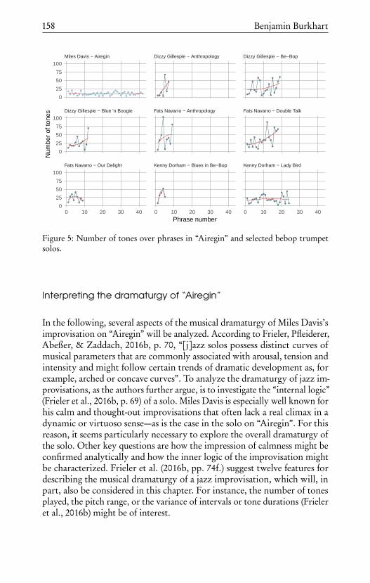
158 Benjamin Burkhart
Fats Navarro − Our Delight Kenny Dorham − Blues in Be−Bop Kenny Dorham − Lady Bird
Dizzy Gillespie − Blue 'n Boogie Fats Navarro − Anthropology Fats Navarro − Double Talk
Miles Davis − Airegin Dizzy Gillespie − Anthropology Dizzy Gillespie − Be−Bop
0 10 20 30 40 0 10 20 30 40 0 10 20 30 40
0
25
50
75
100
0
25
50
75
100
0
25
50
75
100
Phrase number
Num
ber
of to
nes
Figure 5: Number of tones over phrases in “Airegin” and selected bebop trumpetsolos.
Interpreting the dramaturgy of “Airegin”
In the following, several aspects of the musical dramaturgy of Miles Davis’simprovisation on “Airegin” will be analyzed. According to Frieler, Pfleiderer,Abeßer, & Zaddach, 2016b, p. 70, “[j]azz solos possess distinct curves ofmusical parameters that are commonly associated with arousal, tension andintensity and might follow certain trends of dramatic development as, forexample, arched or concave curves”. To analyze the dramaturgy of jazz im-provisations, as the authors further argue, is to investigate the “internal logic”(Frieler et al., 2016b, p. 69) of a solo. Miles Davis is especially well known forhis calm and thought-out improvisations that often lack a real climax in adynamic or virtuoso sense—as is the case in the solo on “Airegin”. For thisreason, it seems particularly necessary to explore the overall dramaturgy ofthe solo. Other key questions are how the impression of calmness might beconfirmed analytically and how the inner logic of the improvisation mightbe characterized. Frieler et al. (2016b, pp. 74f.) suggest twelve features fordescribing the musical dramaturgy of a jazz improvisation, which will, inpart, also be considered in this chapter. For instance, the number of tonesplayed, the pitch range, or the variance of intervals or tone durations (Frieleret al., 2016b) might be of interest.

Mellow Miles 159
Fats Navarro − Our Delight Kenny Dorham − Blues in Be−Bop Kenny Dorham − Lady Bird
Dizzy Gillespie − Blue 'n Boogie Fats Navarro − Anthropology Fats Navarro − Double Talk
Miles Davis − Airegin Dizzy Gillespie − Anthropology Dizzy Gillespie − Be−Bop
0 10 20 30 40 0 10 20 30 40 0 10 20 30 40
0
10
20
30
0
10
20
30
0
10
20
30
Phrase number
Pitc
h ra
nge
Figure 6: Pitch range over phrases in “Airegin” and selected bebop trumpet solos.
Phrases can be understood as rather short and meaningful units with a musicalsense of their own. For each solo in the Weimar Jazz Database, such unitswere annotated manually during the transcription process. When exploringthe musical dramaturgy and the inner logic of a solo, analyzing the successionof musical phrases might be quite helpful, since various musical characteristicsmay differ meaningfully from phrase to phrase. In the solo on “Airegin”,42 phrases in total are annotated. The number of tones contained in eachsingle phrase ranges from three to twenty, the median number is ten. Figure 5illustrates the development over the solo: the number of tones (y-axis) andthe number of phrases (x-axis). The variability is fairly low and, like the meanlength of phrases, does not clearly de- or increase over the course of the solo.When comparing Davis’s variability on “Airegin” with that of the selectedsolos by other bebop trumpeters, one can clearly see the differences (Figure 5).Especially in the rather short solos by Dizzy Gillespie (“Anthropology”),Fats Navarro (“Our Delight”), and Kenny Dorham (“Blues in Bebop”), butalso in Navarro’s longer solo on “Double Talk”, the number of tones overphrases is more variable.
The following analytical features will refer to the musical parameters discussedin the previous section—pitch, interval, and rhythm—in order to contextual-ize the prior findings regarding homogeneity and calmness. Figure 6 providesan overview of the development of pitch range over the 42 phrases of thesolo. The figure illustrates the development over the solo: the number of

160 Benjamin Burkhart
Fats Navarro − Our Delight Kenny Dorham − Blues in Be−Bop Kenny Dorham − Lady Bird
Dizzy Gillespie − Blue 'n Boogie Fats Navarro − Anthropology Fats Navarro − Double Talk
Miles Davis − Airegin Dizzy Gillespie − Anthropology Dizzy Gillespie − Be−Bop
0 10 20 30 40 0 10 20 30 40 0 10 20 30 40
0.0
0.2
0.4
0.6
0.8
0.0
0.2
0.4
0.6
0.8
0.0
0.2
0.4
0.6
0.8
Phrase number
Fuz
zy in
terv
al e
ntro
py
Figure 7: Entropy of fuzzy intervals over phrases in “Airegin” and selected beboptrumpet solos.
tones (y-axis) and the phrase number (x-axis). The minimum pitch rangeover the phrases is three semitones, the maximum sixteen, and the medianrange is thirteen. The variability is again quite low, but the pitch range overthe phrases clearly decreases in the middle of the solo. Additionally, whenreaching the 16 semitone peaks, Davis immediately and clearly reduces thepitch range over the following phrases. As an analysis of improvisations byGillespie, Navarro, and Dorham shows, the differences between the pitchranges over phrases are very apparent. Again, especially in the short solos(e. g., Gillespie’s “Anthropology”), the variability is clearly higher than in“Airegin” (Figure 6). The variability of fuzzy intervals (as explained above)can be analyzed in a similar fashion by calculating the entropy (cf. ChapterComputational melody analysis). Figure 7 was generated by measuring thevariability of interval classes, whereby smaller values indicate lower variabil-ity (Frieler et al., 2016b, p. 75). Therefore, the variability increases slightlyin the second half of the solo. With regard to the other solos, the variabilityis more comparable here than in the foregoing examples. However, Davis’stendency towards smaller values is also apparent.
The variability of the chosen pitches in reference to the underlying chordsmight also be of interest when analyzing the musical dramaturgy. Figure 8illustrates an overview which was created by calculating the entropy (cf. Chap-ter Computational melody analysis) of the distribution of extended chordal

Mellow Miles 161
Fats Navarro − Our Delight Kenny Dorham − Blues in Be−Bop Kenny Dorham − Lady Bird
Dizzy Gillespie − Blue 'n Boogie Fats Navarro − Anthropology Fats Navarro − Double Talk
Miles Davis − Airegin Dizzy Gillespie − Anthropology Dizzy Gillespie − Be−Bop
0 10 20 30 40 0 10 20 30 40 0 10 20 30 40
0.25
0.50
0.75
0.25
0.50
0.75
0.25
0.50
0.75
Phrase number
CD
PC
X e
ntro
py
Figure 8: Entropy of chordal diatonic pitch classes over phrases in “Airegin” andselected bebop trumpet solos.
diatonic pitch classes: In this case, smaller values signify a higher variability(Frieler et al., 2016b, p. 75). As the figure illustrates, there are four obviousoutliers, while the general variability remains quite constant over the courseof the solo. Gillespie’s “Blue ‘n Boogie” and Navarro’s “Double Talk” inparticular are clearly different, since both trumpeters start their improvisa-tions with high values which decrease radically over the following phrases(Figure 8). Furthermore, the development of the duration classes per phrasemust also be mentioned. Similar to the previous figures, smaller values indi-cate a lower variability, since the entropy (cf. Chapter Computational melodyanalysis) of duration classes was calculated (Figure 9; Frieler et al., 2016b,p. 75). There are three clear outliers in the middle of the solo—but as in allother figures, the variation increases at the end of the improvisation. Hence,Davis does not clearly change the phrase durations over the course of theimprovisation. In particular the solos by Gillespie (“Be-Bop”) and Navarro(“Anthropology”) are of higher variability (Figure 9).
In summary: All of the figures concerning “Airegin” depict fairly similarconcave curves. The intensity and variability always decreases slightly untilthe middle of the improvisation, and then increases slightly again until theend of the solo. But in general, the solo appears to be very homogeneous—especially in comparison with more expressive solos in the context of modernjazz and compared to several solos by other bebop trumpeters. All in all,

162 Benjamin Burkhart
Fats Navarro − Our Delight Kenny Dorham − Blues in Be−Bop Kenny Dorham − Lady Bird
Dizzy Gillespie − Blue 'n Boogie Fats Navarro − Anthropology Fats Navarro − Double Talk
Miles Davis − Airegin Dizzy Gillespie − Anthropology Dizzy Gillespie − Be−Bop
0 10 20 30 40 0 10 20 30 40 0 10 20 30 40
0.000.250.500.751.00
0.000.250.500.751.00
0.000.250.500.751.00
Phrase number
Abs
. dur
atio
n cl
ass
entr
opy
Figure 9: Entropy of duration classes over phrases in “Airegin” and selected beboptrumpet solos.
the tools for a dramaturgical analysis confirm the results of the previoussections. That is, the calmness of Miles Davis’s improvisational style canalso be described in terms of statistics. However, one further and importantfeature that cannot be explained by drawing on the statistical tasks outlinedhere is the motivic and melodic development of the improvisation. But thisappears to be a central component, since the solo is played very regularly invarious regards, and too much regularity might even bore listeners.
Midlevel analysis part 1: analyzing the motivic development
The overall structure of an improvisation probably cannot adequately beunderstood if one concentrates solely on certain excerpts of jazz solos—forthis reason, the foregoing section focused on the structural variability of mu-sical phrases over time. The recently developed method of “midlevel analysis”(MLA, Frieler et al., 2016a; Frieler & Lothwesen, 2012; Schütz, 2015) pro-vides an opportunity to explore the motivic structure of an improvisation. Ingeneral, the MLA system encompasses nine main categories, 18 subcategories,and 41 sub-subcategories that are annotated manually to midlevel units. Addi-tionally, the so-called back reference is part of the system. This term describesthe relationship between two or more successive or non-successive midlevelunits within a solo (cf. Chapter Computational melody analysis). Whether two

Mellow Miles 163
units can be described as related to each other is, as is midlevel annotation ingeneral, based on the perception of the annotators. Since relations sometimespass unnoticed, there may be even more references than those actually an-notated. There are various kinds of relationships or references: For instance,musical ideas such as lick can simply be repeated or further developed whilerhythmically or melodically varying just a small excerpt of the foregoingunit. Furthermore, midlevel units can be transposed or varied tonally bychanging the accompanying chords. Additionally, elements of a certain typeof a midlevel unit can be reused in order to create a midlevel unit of anothertype—for example, melodic fragments can form the basis for line MLUs.Miles Davis’s ability to develop and recombine motivic ideas over the entireduration of a single solo has already been highlighted by other researchers(Kerschbaumer, 1978, p. 90). Hence, back references may help to describethese central creative strategies of Davis’s personal style in a quantitativemanner. That is to say, this new approach to studying improvisation mightbe a suitable toolkit for analyzing one of the central components of Davis’spersonal style. For instance, midlevel analysis has already shown remarkabledifferences between Davis and his contemporary John Coltrane (Frieler etal., 2016a, pp. 158f.). In general, this method appears to be highly suitablefor an exploration of Davis’s so-called thoughtful improvisational style.
In “Airegin”, 48 midlevel units in total were annotated by the author of thischapter; 29 musical ideas were labeled as lick, 16 as line, and three as melody(for definitions, see p. 54 and Frieler et al., 2016a, pp. 146f.). Their minimumduration is 0.48 seconds, the maximum 3.59, and the median is 1.45. Theunits contain two to twenty tones, the median number is eight. As for themusical phrases in the previous section, the following figures shall providean overview of the variability of lengths—referring to the number of tones—and durations of the midlevel units (in seconds) during the improvisation(Figure 10, Figure 11).
Once more, the variations are structured quite homogeneously and theyform concave curves. If peaks in duration or length are reached, Davis alwaysimmediately goes back to shorter midlevel units. In general, there are noconspicuous differences between the trends of musical phrases and midlevelunits. In Figure 10, the variations are compared with those of solos played byother bebop trumpeters. Regarding the length (number of tones) of midlevelunits, the graphs do not at first sight show any clear differences in comparisonwith “Airegin”. The variability is predominantly low, as is the case in FatsNavarro’s solo on “Double Talk”, and even decreases over the course ofthe improvisation. Differences become apparent when one compares thelength of individual units. Whereas the longest unit in “Airegin” encompasses20 tones, all the other trumpeters play distinctively longer units up to 77
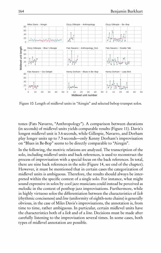
164 Benjamin Burkhart
Fats Navarro − Our Delight Kenny Dorham − Blues in Be−Bop Kenny Dorham − Lady Bird
Dizzy Gillespie − Blue 'n Boogie Fats Navarro − Anthropology_No1 Fats Navarro − Double Talk
Miles Davis − Airegin Dizzy Gillespie − Anthropology Dizzy Gillespie − Be−Bop
0 10 20 30 40 50 0 10 20 30 40 50 0 10 20 30 40 50
0
20
40
60
80
0
20
40
60
80
0
20
40
60
80
Midlevel unit number
Mid
leve
l uni
t len
gth
Figure 10: Length of midlevel units in “Airegin” and selected bebop trumpet solos.
tones (Fats Navarro, “Anthropology”). A comparison between durations(in seconds) of midlevel units yields comparable results (Figure 11). Davis’slongest midlevel unit is 3.6 seconds, while Gillespie, Navarro, and Dorhamplay longer units up to 7.5 seconds—only Kenny Dorham’s improvisationon “Blues in Be-Bop” seems to be directly comparable to “Airegin”.
In the following, the motivic relations are analyzed. The transcription of thesolo, including midlevel units and back references, is used to reconstruct theprocess of improvisation with a special focus on the back references. In total,there are nine back references in the solo (Figure 14, see end of the chapter).However, it must be mentioned that in certain cases the categorization ofmidlevel units is ambiguous. Therefore, the results should always be inter-preted within the specific context of a single solo. For instance, what mightsound expressive in solos by cool jazz musicians could instead be perceived asmelodic in the context of postbop jazz improvisations. Furthermore, whilein highly virtuoso solos the differentiation between the characteristics of lick(rhythmic conciseness) and line (uniformity of eighth-note chains) is generallyobvious, in the case of Miles Davis’s improvisations, the annotation is, fromtime to time, rather ambiguous. In particular, certain midlevel units havethe characteristics both of a lick and of a line. Decisions must be made aftercarefully listening to the improvisation several times. In some cases, bothtypes of midlevel annotation are possible.

Mellow Miles 165
Fats Navarro − Our Delight Kenny Dorham − Blues in Be−Bop Kenny Dorham − Lady Bird
Dizzy Gillespie − Blue 'n Boogie Fats Navarro − Anthropology_No1 Fats Navarro − Double Talk
Miles Davis − Airegin Dizzy Gillespie − Anthropology Dizzy Gillespie − Be−Bop
0 10 20 30 40 50 0 10 20 30 40 50 0 10 20 30 40 50
2
4
6
2
4
6
2
4
6
Midlevel unit number
Mid
leve
l uni
t dur
atio
n (s
)
Figure 11: Duration of midlevel units in “Airegin” and selected bebop trumpet solos.
Miles Davis starts with three licks of similar length and continues with threelines of different subtypes. What follows is an oscillation between one lick,two lines, and again one lick. The following lick, midlevel unit 11 in mm. 23to 24, is the first back reference. The group of six tones is not simply copiedfrom the convex line in mm. 19 and 20, but played at a different metricalposition, and the underlying chords are also different. As a result, the line inbar 20 is reinterpreted as an lick in mm. 23 and 24. In the following, Davisagain plays a mixture of licks and lines. In mm. 46 to 48, he improvises aconvex line which occurs in a similar fashion two units later, in mm. 50 to52, at different metrical positions. After a subsequent concave line, Davisvirtually repeats the first lick of the solo, which functions as an introduction,and ends up in the first bar of the first chorus; the new lick, played in mm.55 to 57, introduces the last A section of the second chorus. That is to say,Miles Davis reuses an idea developed 17 midlevel units before, in the sameharmonic and metrical context. Additionally, the following lick in m. 58 refersto the same idea, as the characteristic interval jump over a fifth is extendedto a sixth. After several more licks and lines, Davis introduces the first moremelodic or cantabile midlevel unit (labeled as melody) in mm. 72 to 74 andfurther develops this idea in the following two bars. The label #+ indicatesthat the idea was partially transposed upwards. The next back reference (mm.88 to 89) is the reinterpretation of the third lick in the solo, which meansthat Davis reuses an idea he introduced 38 midlevel units before. In detail,
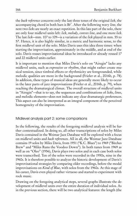
166 Benjamin Burkhart
the back reference concerns only the last three tones of the original lick, theaccompanying chord in both bars is B[7. After the following wavy line, thenext two licks are nearly an exact repetition. In this late part of the solo, thereare only four midlevel units left: lick, melody, convex line, and one more lick.The last lick—mm. 107 to 109—is a variation of the lick played in mm. 55 to57. Hence, it is also highly similar, in a metric and harmonic sense, to thefirst midlevel unit of the solo. Miles Davis uses this idea three times: whenstarting the improvisation, approximately in the middle, and at end of thesolo. Davis reuses improvisational ideas he introduced or already reused 17and 22 midlevel units earlier.
It is important to mention that Miles Davis’s solo on “Airegin” lacks anymidlevel units, such as expressive or rhythm, that might rather create mu-sical tension, since timbral effects or rhythmicity are foregrounded, whilemelodic qualities are more in the background (Frieler et al., 2016b, p. 78).In addition, these types of musical ideas are generally more likely to occurin the later parts of jazz improvisations (Frieler et al., 2016b, p. 79), whenreaching the dramaturgical climax. The overall structure of midlevel unitsin “Airegin”—that is to say, the sequences and combinations of licks, lines,and melodic elements—does not indicate any clear dramaturgic preferences.This aspect can also be interpreted as an integral component of the perceivedhomogeneity of the improvisation.
Midlevel analysis part 2: some comparisons
In the following, the results of the foregoing midlevel analysis will be fur-ther contextualized. In doing so, all other transcriptions of solos by MilesDavis contained in the Weimar Jazz Database will be explored with a focuson midlevel units and back references. All in all, the Weimar Jazz Databasecontains 19 solos by Miles Davis, from 1951 (“K.C. Blues”) to 1969 (“BitchesBrew” and “Miles Runs the Voodoo Down”). In both tunes from 1969 aswell as on “Oleo” (1956), Davis plays two solos and in each case both soloswere transcribed. Ten of the solos were recorded in the 1950s, nine in the1960s. It is therefore possible to analyze the historic development of Davis’simprovisational strategies by comparing older recordings, before the modalimprovisations on Kind of Blue, with solos from the 1960s. At this stage ofhis career, Davis even played rather virtuoso and started to experiment withrock music.
Drawing on the foregoing analytical steps, several graphs illustrate the de-velopment of midlevel units over the entire duration of individual solos. Asin the previous section, there will be two analytical features: the length (the

Mellow Miles 167
1969 − Miles Runs the ...
1969 − Bitches Brew 1969 − Bitches Brew (2) 1969 − Miles Runs the ...
1965 − Agitation 1966 − Dolores 1966 − Orbits
1959 − So What 1964 − E.S.P. 1964 − Eighty−One
1956 − Oleo (2) 1956 − Trane's Blues 1956 − Vierd Blues
1954 − Walkin' 1956 − Blues by Five 1956 − Oleo
1951 − K.C. Blues 1951 − Tune Up 1954 − Airegin
0 20 40 60
0 20 40 60 0 20 40 60
0255075
100
0255075
100
0255075
100
0255075
100
0255075
100
0255075
100
0255075
100
Midlevel unit number
Mid
leve
l uni
t len
gth
Figure 12: Length of midlevel units in all solos by Miles Davis contained in the WeimarJazz Database.
number of tones per unit) (Figure 12) and the duration of midlevel units(in seconds) (Figure 13). The durations are generally comparable with thoseof the solo on “Airegin”. Davis tends to avoid expressive dramaturgical cli-maxes. The graphs further confirm the impression that the uniformity ofmusical ideas over the course of a solo can be considered a central aspect ofMiles Davis’s personal style. One particularly striking example is the solo on“E.S.P.”. In this rather virtuoso improvisation, the durations of midlevel unitshardly de- or increase at all. The analysis of lengths leads to similar results.

168 Benjamin Burkhart
1969 − Miles Runs the ...
1969 − Bitches Brew 1969 − Bitches Brew (2) 1969 − Miles Runs the ...
1965 − Agitation 1966 − Dolores 1966 − Orbits
1959 − So What 1964 − E.S.P. 1964 − Eighty−One
1956 − Oleo (2) 1956 − Trane's Blues 1956 − Vierd Blues
1954 − Walkin' 1956 − Blues by Five 1956 − Oleo
1951 − K.C. Blues 1951 − Tune Up 1954 − Airegin
0 20 40 60
0 20 40 60 0 20 40 60
05
10152025
05
10152025
05
10152025
05
10152025
05
10152025
05
10152025
05
10152025
Midlevel unit number
Mid
leve
l uni
t dur
atio
n (s
)
Figure 13: Duration of midlevel units in all solos by Miles Davis contained in theWeimar Jazz Database.
One recurring feature that was already shown in the analysis of “Airegin”is Davis’s tendency to ultimately reduce the duration or length of musicalideas after reaching conspicuous peaks. On the one hand, this leads to zigzagstructures. On the other hand, as in the case of the second solo on “Miles Runsthe Voodoo Down”, there can sometimes be only one clear outlier, whereasall other midlevel units are of comparable, rather short duration. “Miles Runsthe Voodoo Down” further illustrates that Davis significantly lengthenedsome of his ideas in recordings during the late 1960s—the longest midlevelunits contain up to 100 tones in both solos due to fast rhythmic oscillations.

Mellow Miles 169
Table 1: Midlevel back references in solos by Miles Davis in the Weimar Jazz Database.
Solo Year MLU BR BR (%) MD
K.C. Blues 1951 14 1 7.1 1Tune Up 1951 39 4 10.3 13Airegin 1954 48 9 18.8 38Walkin’ 1954 49 6 12.2 1Blues by Five 1956 63 1 20.6 2Oleo (1) 1956 21 5 23.8 2Oleo (2) 1956 22 4 18.2 2Trane’s Blues 1956 36 10 27.8 16Vierd Blues 1956 24 3 12.5 1So What 1959 27 8 29.6 1E.S.P. 1964 67 11 16.4 60Eighty One 1964 39 6 15.4 5Agitation 1965 41 14 34.2 19Dolores 1966 44 3 6.8 1Orbits 1966 32 1 3.1 1Bitches Brew (1) 1969 39 3 7.7 2Bitches Brew (2) 1969 40 21 52.5 24Miles Runs the Voodoo Down (1) 1969 48 12 25.0 10Miles Runs the Voodoo Down (2) 1969 30 7 23.3 10
Note. MLU = count of midlevel units, BR = count of back references,MD =maximum distance.
As demonstrated in the analysis of “Airegin”, it seems worthwhile to exploreDavis’s usage of back references, too. Table 1 provides an overview of backreferences in all 19 solos by Davis contained in the Weimar Jazz Database.Back references do occur in every solo, but to a varying degree. In the solo on“Orbits”, the percentage of back referenes in relation to all midlevel units isonly 3.1, whereas in the second solo on “Bitches Brew” it is 52.5. Furthermore,in several solos Davis simply develops ideas introduced one unit before, butin “E.S.P.” he refers back to an idea he played as many as 60 units earlier. Allin all, 19.2 % of all midlevel units in the solos analyzed are based on ideasalready introduced beforehand. The extensive usage of back references canbe described, not as a feature necessarily occurring in every analyzed solo,but as a regularly recurring and sometimes essential feature. These findingsshould be verified by analyzing more solos. Nevertheless, back references
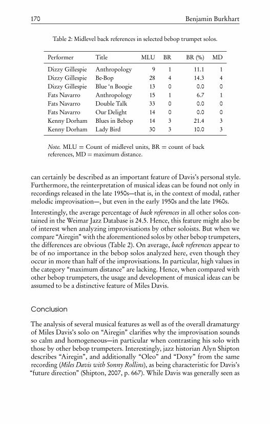
170 Benjamin Burkhart
Table 2: Midlevel back references in selected bebop trumpet solos.
Performer Title MLU BR BR (%) MD
Dizzy Gillespie Anthropology 9 1 11.1 1Dizzy Gillespie Be-Bop 28 4 14.3 4Dizzy Gillespie Blue ‘n Boogie 13 0 0.0 0Fats Navarro Anthropology 15 1 6.7 1Fats Navarro Double Talk 33 0 0.0 0Fats Navarro Our Delight 14 0 0.0 0Kenny Dorham Blues in Bebop 14 3 21.4 3Kenny Dorham Lady Bird 30 3 10.0 3
Note. MLU = Count of midlevel units, BR = count of backreferences, MD =maximum distance.
can certainly be described as an important feature of Davis’s personal style.Furthermore, the reinterpretation of musical ideas can be found not only inrecordings released in the late 1950s—that is, in the context of modal, rathermelodic improvisation—, but even in the early 1950s and the late 1960s.
Interestingly, the average percentage of back references in all other solos con-tained in the Weimar Jazz Database is 24.5. Hence, this feature might also beof interest when analyzing improvisations by other soloists. But when wecompare “Airegin” with the aforementioned solos by other bebop trumpeters,the differences are obvious (Table 2). On average, back references appear tobe of no importance in the bebop solos analyzed here, even though theyoccur in more than half of the improvisations. In particular, high values inthe category “maximum distance” are lacking. Hence, when compared withother bebop trumpeters, the usage and development of musical ideas can beassumed to be a distinctive feature of Miles Davis.
Conclusion
The analysis of several musical features as well as of the overall dramaturgyof Miles Davis’s solo on “Airegin” clarifies why the improvisation soundsso calm and homogeneous—in particular when contrasting his solo withthose by other bebop trumpeters. Interestingly, jazz historian Alyn Shiptondescribes “Airegin”, and additionally “Oleo” and “Doxy” from the samerecording (Miles Davis with Sonny Rollins), as being characteristic for Davis’s“future direction” (Shipton, 2007, p. 667). While Davis was generally seen as

Mellow Miles 171
a bebop trumpeter in the mid-1950s, pieces such as “Airegin” can retrospec-tively be interpreted as early hardbop tunes. Furthermore, the analysis ofthe motivic relations created by Miles Davis illustrates his ‘thoughtful’ styleof improvising. In this specific example, variability seems to be created notby virtuoso lines or expressiveness, but by melodic and motivic references.Therefore, a statistical approach can help to systematically describe and fur-ther understand characteristics of Davis’s (early) personal style that havefrequently been discussed in jazz studies over the last decades. Midlevel anno-tations, in particular, provide deep insights into Miles Davis’s improvisationalstrategies.

172 Benjamin Burkhart
% α α α α 33 Ó − œ œ1
N.C.
q = 241 œ œ œ œ ιœµ ‰ œ ιœ Œ − Ιœ Œ −
2
F m7
ιœ Œ ιœµ ‰ œµ ΙœC 7(∀ 9)
−œ Ιœ œ œ ŒF m7
% α α α α4 ∑F 7( α 9)
Œ Ιœ ‰ ˙B αm7
−œ Ιœ Œ Ιœ ‰F 7(∀ 9)
‰ œµ œ œ œ ÓB αm7
∑
% α α α α9 Œ œ œ œ œ œ œD αmaj7
‰ œµ œ œ œµ œµ œ œD m7 G 7
œµ œµ œ œ œµ œµ œ ‰C maj7
Ó Ιœ œ∀ œµ œα œD αm7 G α7
œµ œµ ˙α ŒB maj7
% α α α α14 Œ œµ œ œ œ œµ œC m7 F 7
œ œµ œ œ œµ œ œ Œ3B αmaj7
Ó − ‰ Ιœ œ œ Ιœ Œ −B αm7
œ œ œ œ œ œ œEα7
% α α α α19 Œ − œµ œ œ œ œ œA αmaj7
œ œ œ œ œ œ œµ œG ø C 7
˙ Ιœ ‰ œF m7
−œµ Ιœ ÓC 7(∀ 9)
Ó œ œ œ œF m7
% α α α α24
œ œ Œ ÓF 7( α 9)
−œ ‰ −œ ιœµB αm7
œ œ œ∀ œµ œ œF 7(∀ 9)
œ Ó −B αm7
Ó − ‰ Ιœ
% α α α α29 ‰ Ιœ ‰ ιœ œ œD αmaj7
−œ Ιœ ÓD ø G 7
‰ œ œ œ œ œ œ œ œ3
3C ø G α7
œ Ιœµ Œ − ≈ œ œF 7 B 7
‰ Ιœ ‰ ιœ œ œB αm7
% α α α α34 −œ Ιœ Ólick
Eα7
Ó œ œ œ œA α6
œ œµ œα œ œµ Œ − œµ œ3
G ø C 7
−œ œµ œ −œ œ œF m7
−œ Ιœ œ œµ ŒC 7(∀ 9)
% α α α α39
œ œµ œ œ œ œ ŒF m7
Ó − ‰ − θœµF 7( α 9)
œ œ œµ œ œ œ Ιœ ≈ Θœline_ascending
B αm7
œ ˙ œµ~lick
F 7(∀ 9)
œ ˙ ŒB αm7
% α α α α44 œ œ Ιœ Œ −lick
lick
∑D αmaj7
‰ œµ œ œ œµ œµ œ œ line convex
##-line convex
D m7 G 7
œµ œµ œ œ œµ œC maj7
ιœ ‰ Ó −D αm7 G α7
% α α α α49 ‰ œ œ∀ ‰ œ ιœα ‰B maj7
Ó − œ œC m7 F 7
œµ œ œ œµ − −œ ΘœB αmaj7
œµ ˙ ιœ ‰ Œ œ œ œ œ œ œµline concave
B αm7
lick lick
lick
line wavy line tick
line wavy lick line descending
line convex ~lick #lick
lick
lick lick ##lick
line tick lick
Figure 14: Transcription with midlevel annotations of Miles Davis’s solo on “Airegin”.

Mellow Miles 173
% α α α α54
œ œ œ œ Ιœ Œ −Eα7
−œ ιœ œ œ œ œA αmaj7
œ œ œ œ œµ œG ø C 7
−œ Ιœ ÓF m7
−œµ Ιœ ÓC 7(∀ 9)
% α α α α59
Ιœ ‰ Ιœ ‰ −œ ΙœF m7
œ œ œ ‰ ÓF 7( α 9)
Œ Ιœ ‰ Ιœ ‰ Ιœ ‰B αm7
−œ Ιœ ‰ − θœ ιœ ‰F 7(∀ 9)
Ιœ ‰ Ιœ ‰ −œ ΙœB αm7
% α α α α64 œ œ ‰ Ιœ ‰ Ιœ Œ Ó − œ œD αmaj7
œ œ œ œ œµ œ œ œµD ø G 7
Θœ ≈ Ιœ œ œµ œα œ œµ Œ3
4C ø G α7
−œ Ιœµ ÓF 7 B 7
% α α α α69 œµ œ ‰ ιœ Œ − ιœB αm7
œ œ œ œ œ œµ œ œµEα7
œ œ Œ ιœ Œ −A α6
Œ − ιœµ œµ œ −œ œµG ø C 7
œ œ ˙F m7
% α α α α74
œ ˙µ œC 7(∀ 9)
‰ − θœ œ −œ ιœF m7
œ −œ Œ −F 7( α 9)
Œ Ιœ œ œ ιœµB αm7
œ œ œ œ œµF 7(∀ 9)
% α α α α79
−œ ‰ ÓB αm7
∑lick
‰ œ œ œ œ œ œ ‰line ascending
line wavyD αmaj7
œ œ œµ œα œ œ œ œµline tick
~lick
D m7 G 7
œ œ ‰ Ó −#38 lick
C maj7
% α α α α84 ∑D αm7 G α7
‰ ιœµ œ −œ ‰line wavy
B maj7
‰ œ œ œ œµ œ œ œαC m7 F 7
œ œµ œ œ œ œlick
B αmaj7
œ Œ Ιœ ‰ œ œ
% α α α α89 ‰ − θœ œ œ ÓB αm7
œ œ œ œ Ιœ ‰ œµ œµEα7
œ œ −œ œµ œ œ œα œA αmaj7
Œ œ œ œ œ œG ø C 7
ιœ ‰ −œ Œ −F m7
% α α α α94 Œ œ œ −œ Ιœ#lick
C 7(∀ 9)
œ œ Œ œ ŒF m7
∑F 7( α 9)
Ιœ ‰ œ œ œµlick
B αm7
œ ‰ Ιœ −œ ΙœF 7(∀ 9)
Ιœ ‰ −œ Œ −B αm7
% α α α α100 ∑line convex
‰ Ιœ Œ ˙D αmaj7
Ιœ ‰ œ œ œmelody
#22-lickD ø G 7
−œ −œ ‰ ιœαC ø G α7
œ −œ Œ −F 7 B 7
% α α α α105 Œ œ œ œ œ œ œB αm7
œ œ œ œµ œα œµ œα œEα7
ιœ Ó ιœ œ œA α6
œ œ œ œ œ œµG ø C 7
−œ ‰ ÓF m7
#17 lick #-lick
lick lick
line tick lick
lick melody
#+melody lick
Figure 14: (Continued).


West Coast lyricists:Paul Desmond and Chet Baker
Benjamin Burkhart
The term “West Coast jazz” itself often occurs in jazz historiography, eventhough there is no general agreement as to what it exactly refers to. Thequestion of whether it can be characterized as a distinctive musical style or, asjazz critic and researcher Ted Gioia puts it, merely “a somewhat unified phe-nomenon” (Gioia, 1992, p. 363) often arises. This chapter explicitly does notaim at answering this question, but instead focuses analytically on musicianssuch as Chet Baker and Paul Desmond who are generally acknowledged to beamong the most prominent protagonists of West Coast jazz—either becauseof their origins or because of their long-term activities in the western part ofthe US, principally Los Angeles and San Francisco. The focus will be on acomparison between their personal improvisational styles, with reference toanalytical writings published on West Coast jazz up till now. One main goalis to explore characteristics often associated with West Coast jazz musiciansand to provide a foundation for further analytical research.
In terms of public attention and commercial success, West Coast jazz wasthe most popular jazz style since the swing era. In the first half of the 1950s,musicians such as Gerry Mulligan and Dave Brubeck formed ensembleswhich soon attracted national attention. Hence, it is hardly surprising thatthe West Coast stars were criticized by journalists and jazz musicians alikefor their alleged commercialism or musical primitivism. One key aspect indiscussions of West Coast jazz is the assumption that it somehow deviatedfrom the cool jazz of the East Coast, mainly New York City. Generallydescribed as a ‘Euro-American’ equivalent to ‘African-American’ cool jazz inthe tradition of Miles Davis, several sociocultural influences are believed to beessential for the development of West Coast jazz. Being based in California,mainly in Los Angeles, many jazz musicians profited from an artistic and
176 Benjamin Burkhart
economic infrastructure that was distinctly different from that of the EastCoast. Thanks to the recording studios of Hollywood and a number ofbig bands and orchestras, musicians often had the opportunity to be paidrelatively well for their work—as a result, working as a jazz musician on theWest Coast was described as a regular employment rather than an artistic,creative activity (Hellhund, 1985, p. 240; Jost, 2003, pp. 160–171).
According to Ekkehard Jost, the employment of jazz musicians in big bandsand orchestras further led to an unusual degree of musical standardization.To be a member of these big ensembles, one had to fulfill certain criteriarelating to instrumental sound, since the music was an integral part of Califor-nia’s cultural industry—people wanted to hear the sound they already knewand appreciated. Furthermore, pianist Stan Kenton’s big band was of greatsignificance for West Coast jazz. Kenton in particular tried to create a ‘Euro-pean’ sounding version of contemporary jazz, one influenced by symphoniccompositions by, for instance, Richard Strauss, Nikolai Rimsky-Korsakov, orSergei Prokofiev (Jost, 2003, pp. 158–162). However, West Coast jazz becamefamous not for its big bands and orchestras but for the small ensembles ofGerry Mulligan and Dave Brubeck, and for instrumentalists such as ChetBaker, even though most of the musicians were former members of the largeHollywood ensembles. According to Herbert Hellhund, the music of thesmall ensembles can be characterized by distinctly non-virtuoso and rathercantabile improvisations and by technical sophistication in arrangements andensemble playing. Furthermore, Hellhund believes that the various synthesesof musical styles of African-American and European descent are significantfor West Coast jazz (Hellhund, 1985, pp. 236–241). Ted Gioia further notesthat the sound of West Coast jazz “was cleanly articulated, the executionfluid and polished” (Gioia, 1992, p. 362). Among the most prominent in-strumentalists who became well-known especially for their melodic, lyricalimprovisations are the alto-saxophonist Paul Desmond and the trumpeterChet Baker. The analysis of these two musicians forms the basis of this chap-ter, since they appear to be directly comparable. Additional comparisons withother musicians generally associated with West Coast jazz, Gerry Mulligan,Stan Getz, and Zoot Sims, are also undertaken in order to contextualize thefindings. In a last step, solos by East Coast cool jazz instrumentalists (LeeKonitz, Warne Marsh) are analyzed in order to compare aspects of West andEast Coast jazz.

West Coast lyricists 177
“The world’s slowest alto player”—Paul Desmond
A description like “the world’s slowest alto player” might seem quite unflat-tering—however, it is a description formulated not, as one might think, byjournalists or resentful musicians, but by Paul Desmond himself. And indeed,Desmond, who became especially well-known for his collaboration withpianist Dave Brubeck and for his composition “Take Five” (1959), does notseem directly comparable with the virtuoso alto style of the 1940s and 1950spopularized by Charlie Parker and his fellows. Nevertheless, he is assumed tobe one of the most well-known alto players of the 1950s and 1960s, referringdirectly to the style of saxophonists such as Lester Young or Benny Carter inthe two foregoing decades (Harrison & Kernfeld, 2001, p. 605).
Desmond began his career as a professional musician when studying the clar-inet at San Francisco Polytechnic; in 1943, he switched to the alto saxophone.After being drafted into the army, he worked as a military musician and waspart of the 253rd AGF (Army Ground Forces) Band. In the following years,he was first hired to play in Alvino Rey’s and Jack Fina’s ensembles beforeworking with Dave Brubeck. He was a member of Brubeck’s famous quartetfrom 1951 to 1967. Besides his collaboration with Dave Brubeck, Desmondreleased several recordings with musicians such as Gerry Mulligan, Jim Hall,Chet Baker, and the Modern Jazz Quartet (Gioia, 1992, p. 77).
Even though Desmond’s work has largely been ignored by academia up untilnow, some of his contemporaries describe him as one of the most centralfigures in jazz during the 1950s and 1960s. Dave Brubeck states:
Of all the alto saxophonists of his day, so under the influenceof Charlie Parker, Paul was the one who struck his own pathand found his own sound, integrating in his improvisations agreat sense of melody, harmonic and rhythmic invention—andwit (cited from Ramsey et al., 2005, p. 11).
Musicologist Thomas Owens further describes Desmond as being one ofthe “three most prominent non-members of the Parker school”, besidesArt Pepper and Lee Konitz (Owens, 1995, p. 2). Not being part of the so-called ‘Parker school’ means that the alto saxophonist was among those jazzmusicians who created musical styles that deviated from the bebop idiomof the late 1940s and early 1950s. Ted Gioia even assumes that Desmondhad “perfected a ‘cool’ alternative to the bebop style” (Gioia, 1992, p. 122).But at the same time, he describes Desmond as “a saxophonist who seemedcompletely out of touch with musical modernism” (Gioia, 1992, p. 69) andwho had polished “a retrograde, almost anti-modern saxophone style“ (Gioia,1992, p. 75).
178 Benjamin Burkhart
What Gioia both praises and criticizes is the probably most prominent fea-ture of Desmond’s personal style: the melodic, rather simple improvisationsthat clearly distinguish him from the virtuosity of jazz musicians associatedwith the aforementioned ‘Parker school’. Most of the authors who have pub-lished biographical or analytical works on Paul Desmond highlight the altoplayer’s melodic inventiveness (Harrison & Kernfeld, 2001, p. 605; Kunzler,2002, p. 292), or again in Gioia’s words: his “talent for melodic construction”(Gioia, 1992, p. 90). According to Günter Gliesche, Desmond played jazz likea thinking person with lyrical intelligence, and improvised clear and melodiclines (Gliesche, 2006, p. 9). In his analytical study on cool and West Coastjazz, musicologist Herbert Hellhund further highlights Desmond’s simple,motivic style which, according to the author, led to highly structured andcontinuous improvisations (Hellhund, 1985, pp. 259f.). One other strikingand frequently mentioned feature is Desmond’s personal sound. When at-tempting to describe Desmond’s sound, adjectives such as “lyrical”, “tender”,“airy”, “romantic” (Kunzler, 2002, p. 292), “lucid”, or “bright” (Gioia, 1992,p. 90) are used. In summing up, biographer Dough Ramsey states that PaulDesmond was “famous for the warmth, inventiveness and lyricism of hisplaying“ (Ramsey et al., 2005, p. 13).
The writings mentioned above demonstrate that Paul Desmond’s melodicallyinventive and motivic improvisations are among the most distinctive featuresof his personal style. Even though this talent is frequently highlighted by anumber of authors, Desmond’s technical abilities are generally described asbeing quite limited. The parallels to writings on Chet Baker are obvious, sinceBaker is acknowledged to be another great melodic improviser of so-calledWest Coast jazz.
“There’s a little white cat out on the West Coast who’s gonnaeat you up”—Chet Baker
This section heading refers to a quote attributed to Charlie Parker. Accordingto Chet Baker himself, Parker had warned Miles Davis and Dizzy Gillespieafter having played a short tour on the West Coast with Baker—a tour thatis generally acknowledged as being a breakthrough in Baker’s career (Gioia,1992, p. 172). As a child, Baker started playing music on the trombone beforeswitching to the trumpet at the age of thirteen. Like Paul Desmond, Bakerbecame a military musician in the 1940s. In 1946, he first joined the 298thArmy Band in Berlin, and then the Presidio Army Band in San Franciscoin 1948. After being discharged in 1952, Baker intermittently played localjobs until he first met Charlie Parker at an audition hosted by Parker in

West Coast lyricists 179
Los Angeles (Gordon, 1986, p. 72). At that time, Baker was already highlyinterested in the music of trumpeters such as Miles Davis, Fats Navarro, andRed Rodney (Gioia, 1992, p. 170). Miles Davis in particular is believed tohave had a huge influence on Chet Baker. But, as Alain Tercinet assumes,Baker had already developed some highly characteristic elements of his ownpersonal style before becoming more and more inspired by Davis (Tercinet,1986, p. 95). That is to say, it might be difficult to decide which trumpeterinfluenced the other to what degree at any given time. In 1952, Baker andbaritone saxophonist Gerry Mulligan formed their famous quartet and Bakerbecame well-known as a solo artist with his later groups, too (Gordon, 1986,p. 82).
Like Paul Desmond, Baker deviated from the virtuoso solo style of the bebopera. According to Robert Gordon, his style as a trumpeter was dominated by“a tendency towards introspection, a limited emotional range”—somethingGordon further characterizes as the “very worst faults of Baker’s trumpetstyle” (Gordon, 1986, p. 83). Gordon was not the only writer to criticizeBaker’s technical abilities. Jeroen de Valk assumes the expressivity of Baker’splaying to be his key talent, whereas in a technical sense, he calls him an“[a]nalphabet” (Valk, 1991, p. 15). But Ted Gioia also highlights Chet Baker’sability to deal with his technical limitations and to thereby create a distinctivestyle of playing:
[H]e did so much with his limited musical tools that one scarcelykept track of what he couldn’t or didn’t do. In an age of incessantvirtuosity, Baker’s work was a telling and much-needed reminderthat technical mastery was not the only path to musical expres-sion, and indeed could often be a beguiling dead-end street (Gioia,1992, p. 169).
As in the case of Paul Desmond, Baker’s playing has been described as “un-commonly lyrical” (Gioia, 1992, p. 181). Alain Tercinet further states thatChet Baker’s improvisations were characterized by a “disenchanted lyricism”(“lyrisme désenchanté”) (Tercinet, 1986, p. 95) and had an “intimate andromantic character” (“charactère intimiste et romantique”) (Tercinet, 1986,p. 234). Furthermore, his contemporaries highlight his ability to react intu-itively to new or unfamiliar musical situations, as stated by Gerry Mulligan(Valk, 1991, p. 35). According to Mulligan, Baker could not even read sheetmusic and played everything by ear (Gioia, 1992, p. 174). Herbert Hellhundfurther praises Baker’s talent for melodic inventiveness and states that thisability led to an “atmospheric intensity” (“atmosphärische[n] Intensität”)(Hellhund, 1985, p. 264).

180 Benjamin Burkhart
What therefore seems interesting about the improvisational styles of PaulDesmond and Chet Baker is their melodic and technically limited but nonethe-less—according to the authors quoted above—lyrical playing. The followingsections aim particularly at exploring and comparing these characteristicsin improvisations by both musicians. Furthermore, the results are contex-tualized by analyses of selected solos by other jazz musicians commonlyassociated with West and East Coast cool jazz.
Analyzing pitch classes
The Weimar Jazz Database contains eight solos each by Desmond and Baker.Six of Desmond’s tunes were released on his album Bossa Antigua (1964); heplayed two solos on “Alianca” and “Samba Cantina” and in each case, bothsolos were transcribed. Two more solos are from “Blue Rondo a la Turk” and“The Girl from East 9th Street”, which appeared on the album Time Out(1959) by the Dave Brubeck Quartet. Six of Baker’s solos were recorded inthe mid-1950s (1954/1955), whereas his improvisations on “Two’s Blues” and“You’d Be So Nice to Come Home to” are from 1975. Most of Desmond’ssolos are played on bossa nova pieces. The available recordings of Chet Bakerare more heterogeneous, ranging from the slow ballad “I Fall in Love TooEasily” (1954) to the up-tempo tune “You’d Be So Nice to Come Home to”.
In order to gain an impression of the degree of harmony or consonance,the distribution of pitch classes—diatonic or consonant vs. chromatic ordissonant pitches—will be analyzed. The following histograms provide anoverview of the (extended) chordal diatonic pitch class distribution—that is,the diatonic and non-diatonic pitches according to the root of the underlyingchord—in all solos by the two musicians, in total (Figure 1) and per tune(Figure 2). In the case of Paul Desmond, the fifth is the pitch class played mostoften, followed by the third and the root note. Chet Baker, on the other hand,emphasizes the root note, the fifth, and the fourth. But the pitch distributionper solo also illustrates that there are only a few obvious preferences forcertain pitch classes in both musicians’ improvisations. Interestingly enough,Desmond and Baker often focus on the third (Desmond: “Alianca (1)”, “AloneTogether”, “Samba Cantina (1)”, “Samba Cantina (2)”; Baker: “Long Agoand Far Away”, “Two’s Blues”, “You’d Be So Nice to Come Home to”),which indicates a highly consonant melodic structure that emphasizes theunderlying chords. On the other hand, Desmond sometimes emphasizes thesecond and fourth (“Bossa Antigua”), and Baker even the sixth and seventh(“Just Friends”) or fourth (“Let’s Get Lost”, “There Will Never Be AnotherYou (1)”). Hence, there are no overall preferences in either musicians’ solos.
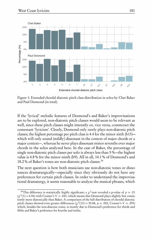
West Coast lyricists 181
Paul Desmond
Chet Baker
1 2 3 4 5 6 7 #9 #7 #11 b7 #1
0 b9 b13
0%
5%
10%
15%
0%
5%
10%
15%
Extended chordal diatonic pitch class
Per
cent
age
(%)
Figure 1: Extended chordal diatonic pitch class distribution in solos by Chet Bakerand Paul Desmond (in total).
If the ‘lyrical’ melodic features of Desmond’s and Baker’s improvisationsare to be explored, non-diatonic pitch classes would seem to be relevant aswell, since these pitch classes might intensify or, vice versa, counteract theconsonant ‘lyricism’. Clearly, Desmond only rarely plays non-diatonic pitchclasses; the highest percentage per pitch class is 4.4 for the minor sixth (b13)—which will only sound (mildly) dissonant in the context of major chords or amajor context—, whereas he never plays dissonant minor sevenths over majorchords in the solos analyzed here. In the case of Baker, the percentage ofsingle non-diatonic pitch classes per solo is always less than 5 %—the highestvalue is 4.8 % for the minor ninth (b9). All in all, 14.1 % of Desmond’s and18.2 % of Baker’s tones are non-diatonic pitch classes.16
The next question is how both musicians use non-diatonic tones or disso-nances dramaturgically—especially since they obviously do not have anypreferences for certain pitch classes. In order to understand the improvisa-tional dramaturgy, it seems reasonable to analyze the musical phrases, which
16This difference is statistically highly significant; a χ 2-test revealed a p-value of p = .01(χ 2(1) = 6.54) with Cramer’s V = .043, which means that Desmond plays slightly but consis-tently more diatonically than Baker. A comparison of the full distribution of chordal diatonicpitch classes showed even greater differences (χ 2(13) = 30.68, p = .002, Cramer’s V = .093)which, besides the non-diatonic tones, is mostly due to Desmond’s preference for thirds andfifths and Baker’s preference for fourths and sixths.

182 Benjamin Burkhart
Paul Desmond − Samba Cantina−2 Paul Desmond − The Girl from East 9th Street
Paul Desmond − Bossa Antigua Paul Desmond − Samba Cantina
Paul Desmond − Alone Together Paul Desmond − Blue Rondo a la Turk
Paul Desmond − Alianca Paul Desmond − Alianca−2
Chet Baker − Two's Blues Chet Baker − You'd Be So Nice to Come Home to
Chet Baker − There Will Never Be Another You Chet Baker − There Will Never Be Another You−2
Chet Baker − Let's Get Lost Chet Baker − Long Ago and Far Away
Chet Baker − I Fall in Love Too Easily Chet Baker − Just Friends
1 2 3 4 5 6 7 #9 #7 #11 b7 #1
0 b9 b13 1 2 3 4 5 6 7 #9 #7 #1
1 b7 #10 b9 b1
3
0%5%
10%15%20%25%
0%5%
10%15%20%25%
0%5%
10%15%20%25%
0%5%
10%15%20%25%
0%5%
10%15%20%25%
0%5%
10%15%20%25%
0%5%
10%15%20%25%
0%5%
10%15%20%25%
Extended chordal diatonic pitch class
Per
cent
age
(%)
Figure 2: Extended chordal diatonic pitch class distribution in solos by Chet Bakerand Paul Desmond (per tune).

West Coast lyricists 183
were annotated manually for each solo contained in the Weimar Jazz Data-base. Phrases, which can be understood as fairly short and meaningful unitswith a musical sense of their own, can help to understand the “internal logic”(Frieler et al., 2016b, p. 69) of jazz improvisations by allowing one to examinethe variation of musical features over phrases. The following graphs illustratethe development of playing non-diatonic tones over phrases in the solos ofPaul Desmond and Chet Baker (Figure 3). There, the phrase-wise percentageof non-diatonic tones is depicted along with quadratic polynomial trend lines.
In the case of Desmond, there are various strategies for playing dissonancesover phrases. Ongoing variations lead to zigzag curves (“Alianca (1)”, “AloneTogether”, “Blue Rondo A La Turk”), convex curves (“Alianca (2)”, “BossaAntigua”, “Samba Cantina (2)”), and low variability with few outliers (“SambaCantina (1)”, “The Girl From East 9th Street”). In Baker’s solos, there areconvex curves (“I Fall in Love Too Easily”, “There Will Never Be AnotherYou (1)”), strongly increasing trend lines (“Let’s Get Lost”, “Long Ago AndFar Away”), and examples with low variability (“Just Friends”, “There WillNever Be Another You (2)”, “You’d Be So Nice to Come Home to”).
In the following, both musicians’ strategies for playing non-diatonics arecompared. In doing so, it is fairly essential to choose comparable examples.First of all, solos played on comparatively slow and balladic tunes, which atthe same time display certain distinctive features regarding outliers or trendlines, are selected. Desmond’s first improvisation on “Samba Cantina” is oneof the slower solos contained in the Weimar Jazz Database; the average tempois 150.8 bpm. The structure of non-diatonic playing is quite conspicuous,since there are several phrases without any chromatic pitch classes at all, aswell as obvious outliers (up to 70 %). Chet Baker’s “I Fall in Love Too Easily”is by far the slowest tune among the selected recordings (65.2 bpm) and, as in“Samba Cantina”, there is a pendulum structure of non-diatonic and diatonicphrases—whereas the convex trend lines clearly differ from those in the figurereferring to Desmond’s solo. The strategies of playing diatonically or non-diatonically over phrases can be explored by analyzing both the percentageof non-diatonic pitch classes and the number of tones per phrase. In doingso, the focus is on whether the soloists choose non-diatonic pitch classesin short phrases, thereby creating attention for brief moments only, or ifthe non-diatonics are played over longer passages. In this case, it could beargued that non-diatonic tones are highlighted as more integral elements ofthe overall dramaturgy.
Figure 4 illustrates the percentage of non-diatonic pitch classes and the num-ber of tones for each phrase in Paul Desmond’s first solo on “Samba Cantina”.First of all, the trend lines are clearly reversals of one another—convex for non-

184 Benjamin Burkhart
Paul Desmond − The Girl from East 9th...
Paul Desmond − Samba Cantina Paul Desmond − Samba Cantina−2
Paul Desmond − Blue Rondo a la Turk Paul Desmond − Bossa Antigua
Paul Desmond − Alianca−2 Paul Desmond − Alone Together
Chet Baker − You'd Be So Nice to Come... Paul Desmond − Alianca
Chet Baker − There Will Never Be Anot... Chet Baker − Two's Blues
Chet Baker − Let's Get Lost Chet Baker − Long Ago and Far Away
Chet Baker − I Fall in Love Too Easily Chet Baker − Just Friends
0 10 20 30
0 10 20 30
0%20%40%60%
0%20%40%60%
0%20%40%60%
0%20%40%60%
0%20%40%60%
0%20%40%60%
0%20%40%60%
0%20%40%60%
Phrase number
Non
−D
iato
nics
(%
)
Figure 3: Non-diatonic tones over phrases in solos by Chet Baker and Paul Desmond.

West Coast lyricists 185
Chet Baker − I Fall in Love Too Easily Paul Desmond − Samba CantinaN
on−D
iationicsN
ote Count
Syncopicity
Duration E
ntropy
0 5 10 15 20 0 5 10 15 20
0.0
0.2
0.4
0.6
10
20
30
40
0.0
0.2
0.4
0.6
0.8
0.00
0.25
0.50
0.75
Phrase number
Figure 4: Non-diatonic tones, number of tones, syncopicity, and duration entropyover phrases in Chet Baker’s solo on “I Fall in Love Too Easily”, and Paul Desmond’sfirst solo on “Samba Cantina”.
diatonic tones and concave for the number of tones per phrase. Desmond’sfirst three phrases are relatively short, and as the percentage of non-diatonictones is zero twice, it could be argued that he improvises very consonantly.In phrases four and five, both trend lines display the same direction, whereasin the following phrases up until number eleven, the directions are some-times opposed. Additionally, the next dissonance peak in phrase 17 is notaccompanied by a strong increase in the number of tones. In contrast, thedirections of both trend lines over the last three phrases are quite similar. Butas in the case of phrase 8 or 19, Desmond sometimes plays comparativelylong phrases of 20 tones or more without any non-diatonic pitch classes. Thatis to say, he uses rather long phrases to play fairly consonantly rather thancreate tonal tension or smooth out his lines with chromatic passing tones.Figure 5 illustrates an example of a long diatonic phrase. The melodic qualitymight be attributed to the four-eighth-note pattern which Desmond repeatsthree times in bars 21 and 22. Desmond repeats a pendulum between theminor seventh, minor third, minor seventh, and fifth in bar 21, and betweenthe fourth, minor seventh, fourth, and second in bar 22.
Figure 4 also illustrates the development over phrases in Chet Baker’s soloon “I Fall in Love Too Easily”. In this case, the trend lines look fairly similar.Baker starts with a phrase without any non-diatonic pitch classes, whereas in
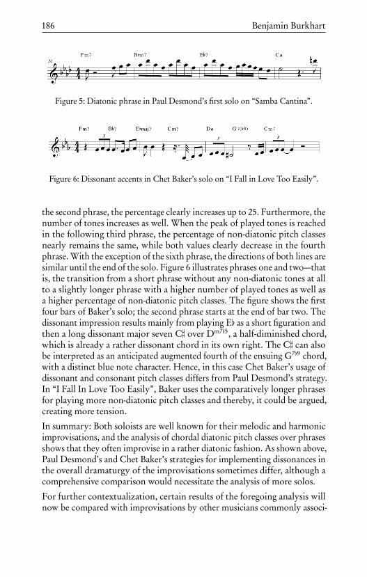
186 Benjamin Burkhart
Figure 5: Diatonic phrase in Paul Desmond’s first solo on “Samba Cantina”.
Figure 6: Dissonant accents in Chet Baker’s solo on “I Fall in Love Too Easily”.
the second phrase, the percentage clearly increases up to 25. Furthermore, thenumber of tones increases as well. When the peak of played tones is reachedin the following third phrase, the percentage of non-diatonic pitch classesnearly remains the same, while both values clearly decrease in the fourthphrase. With the exception of the sixth phrase, the directions of both lines aresimilar until the end of the solo. Figure 6 illustrates phrases one and two—thatis, the transition from a short phrase without any non-diatonic tones at allto a slightly longer phrase with a higher number of played tones as well asa higher percentage of non-diatonic pitch classes. The figure shows the firstfour bars of Baker’s solo; the second phrase starts at the end of bar two. Thedissonant impression results mainly from playing E[ as a short figuration andthen a long dissonant major seven C] over Dm7[5, a half-diminished chord,which is already a rather dissonant chord in its own right. The C] can alsobe interpreted as an anticipated augmented fourth of the ensuing G7[9 chord,with a distinct blue note character. Hence, in this case Chet Baker’s usage ofdissonant and consonant pitch classes differs from Paul Desmond’s strategy.In “I Fall In Love Too Easily”, Baker uses the comparatively longer phrasesfor playing more non-diatonic pitch classes and thereby, it could be argued,creating more tension.
In summary: Both soloists are well known for their melodic and harmonicimprovisations, and the analysis of chordal diatonic pitch classes over phrasesshows that they often improvise in a rather diatonic fashion. As shown above,Paul Desmond’s and Chet Baker’s strategies for implementing dissonances inthe overall dramaturgy of the improvisations sometimes differ, although acomprehensive comparison would necessitate the analysis of more solos.
For further contextualization, certain results of the foregoing analysis willnow be compared with improvisations by other musicians commonly associ-

West Coast lyricists 187
Table 1: Phrase lengths (number of tones) in solos by West and East Coast jazzmusicians.
Soloist Median Range
Paul Desmond 12 2–63Chet Baker 14.5 1–63Gerry Mulligan 18 2–65Stan Getz 14 2–71Zoot Sims 13 3–48Lee Konitz 24 3–79Warne Marsh 24 2–66
ated with West Coast jazz. For the comparisons, solos by Gerry Mulligan,Stan Getz, and Zoot Sims are taken into consideration. Furthermore, solosby Lee Konitz and Warne Marsh—East Coast cool jazz musicians in the tra-dition of Lennie Tristano—are analyzed as well, in order to explore possibledifferences between West and East Coast jazz soloists. According to HerbertHellhund, short phrases are especially typical for Paul Desmond’s personalstyle (Hellhund, 1985, p. 258).17 These characteristics were also evident inthe foregoing analysis. For this reason, the number of tones per phrase waschosen as one analytical feature for the comparison with other jazz musicians.The following table lists the median phrase lengths and their range over allthe solos by each musician (Table 1).
As a matter of fact, the median phrase length of Desmond’s solos is thelowest, followed by Sims and Getz. The median length of Baker’s phrasesis slightly higher than Getz’s, whereas Mulligan plays the most tones perphrase compared with the other West Coast players. The median valuesof Konitz’s and Marsh’s solos are both, at 24 tones per phrase, generallyhigher, even twice as high as Desmond’s median value, which can be regardedas a considerable difference. However, the differences with respect to theminimum and maximum values are rather small.18
Furthermore, we will also compare the distribution of chordal diatonic pitchclasses (extended)—summarized for all solos (Figure 7). The root note, the
17This can in fact be corroborated with a t-test (t (105.14) = 2.769, p = .007∗∗), with a meanphrase length of 13.6 tones for Desmond and 18.3 for Baker. Baker also displays a highervariability of phrase lengths (SD = 14.0) than Desmond (SD = 8.43).
18A one-way variance analysis (ANOVA) of phrase lengths by performer revealed highlysignificant differences (F (6,778) = 13.84, p = .000∗∗∗, adj. R2 = .09), with Konitz and Marshplaying much longer and Desmond playing much shorter phrases. Baker is in the middle field.

188 Benjamin Burkhart
Figure 7: Distribution of extended chordal diatonic pitch classes in solos by West andEast Coast jazz musicians.

West Coast lyricists 189
third, fifth, and the seventh are the pitch classes most often played by WestCoast jazz musicians, while the emphasis on the third is also apparent in theirimprovisations. The percentages of non-diatonic pitch classes are slightlyhigher compared to Desmond and Baker: 18.1 % (Gerry Mulligan), 19.6 %(Stan Getz), and 15.4 % (Zoot Sims). Regarding the chordal diatonic pitchclass distribution, the results for Konitz’s and Marsh’s solos do not differsignificantly. The percentages of non-diatonic pitch classes are comparable,too: 17.6 % (Lee Konitz), 14.3 % (Warne Marsh).19
Analyzing rhythm
When analyzing musicians who are acknowledged to be melodic ‘lyricists’,it seems appropriate to concentrate on stylistic features that might reflectrhythmic tension. One can explore how musicians use or don’t use suchfeatures, especially as part of the overall dramaturgy of an improvisation.Syncopicity, i.e., tones on offbeats with no event on the following on-beat,was chosen as a first basic feature that is assumed to create rhythmic tension.20
The following figure provides an overview of the percentage of syncopicityin all solos by Paul Desmond and Chet Baker contained in the Weimar JazzDatabase, and by the other West and East Coast jazz musicians (Figure 8). Thefigure clearly illustrates that, on average, less than half of all tone events aresyncopated events. These results seem obvious in view of the two musicians’calm, lyrical style of improvising. One might assume that they do not try tocreate rhythmic tension by an extensive use of syncopated events.
As in the previous section, the relevance of the analyzed features for theoverall dramaturgy of improvisations is to be explored here, too. Again, theexamples chosen are Desmond’s first solo on “Samba Cantina” and Baker’s“I Fall in Love Too Easily”—the percentage for Baker’s solo is the highest, thevalues for two solos on “Samba Cantina” are the lowest. Figure 4 illustratesthe development of syncopated tone events over phrases. In Desmond’s solo,the peak is already reached in the second phrase (50 %). In the following bars,the percentages of syncopated events oscillate regularly between values ofup to 40 %, which leads to a slightly concave trend line. Chet Baker, on the
19A one-way ANOVA of the number of non-diatonic pitch classes per phrase by performerrevealed a significant effect (F (6,766) = 3.49, p = .002, adj. R2 = .019), with Gerry Mulligan,Stan Getz and Zoot Sims playing slightly more non-diatonic tones than average, and PaulDesmond and Warne Marsh playing fewer. However, the effect is rather small.
20Note that metrical positions in the Weimar Jazz Database are provided by a metrical anno-tation algorithm, which means that not only proper syncopations contribute to the syncopicityvalue, as used here, but also micro-timing aspects, such as laid-back or loose (or sloppy) playing,which might result in higher values.

190 Benjamin Burkhart
Absolute Duration Class Entropy
Event density
Syncopicity
Chet Baker Paul Desmond Gerry Mulligan Stan Getz Zoot Sims Lee Konitz Warne Marsh
0.00
0.25
0.50
0.75
1.00
2.5
5.0
7.5
10.0
12.5
0.00
0.25
0.50
0.75
1.00
Performer
Figure 8: Syncopicity, event density, and absolute duration class entropy in solos byWest and East Coast jazz musicians.
other hand, seems to purposefully make use of syncopicity, since the highestvalue is 80 % and the trend line increases strongly over the course of theimprovisation. While the structure of Paul Desmond’s solo can be describedas relaxed and calm, Baker appears to improvise more ‘expressively’.
The next feature is event density, measured as the number of tones per second.Figure 8 summarizes the event densities of all solos by both musicians, and bythe other West and East Coast musicians. In this case, the differences betweenDesmond and Baker are rather small—the event densities are comparativelylow. What event density cannot explain is rhythmic flexibility. But this mightbe a relevant analytical feature if improvisational calmness is to be explored,especially in a dramaturgical sense. For this reason, the entropy of absoluteduration classes, which measures the variability of duration classes whichare defined in relation to a tempo-independent reference value of 500 ms,was calculated. Here, smaller values indicate lower variability (Frieler et al.,2016b, p. 75). Figure 8 provides an overview of entropies for all solos, Figure 4illustrates the entropy of duration classes over phrases in Desmond’s “SambaCantina” and Baker’s “I Fall in Love Too Easily”. In Desmond’s solo, thevalues oscillate regularly between approximately 0.5 and 0.9, leading to atrend line that decreases slightly in the middle and increases again slightly atthe end of the solo—the variability is quite low. Chet Baker’s solo appears to

West Coast lyricists 191
be more varied, especially due to phrase four, where the entropy is clearlydecreasing. But in general, the values are rather similar (Figure 4).
In summary: Concerning mean values of syncopicity, event density, and dura-tion classes, the improvisations by Paul Desmond and Chet Baker are highlysimilar. The differences become obvious when one explores the dramaturgyand the concordances of different analytical features. Baker appears to bethe more ‘expressive lyricist’. Whether the analytical findings described hereare special in the context of West Coast jazz (and in part that of East Coastjazz as well) will be explored by a comparison with the aforementioned jazzmusicians (Figure 8).
First of all, the percentage of syncopicity was calculated for each solo. WestCoast jazz instrumentalists Stan Getz and Zoot Sims play distinctly moresyncopations, whereas Lee Konitz and Warne Marsh clearly play fewer syn-copated tone events—probably due to the higher amount of fast eighth-notechains. Baker, Desmond and Mulligan are located in between the extremes. Incomparison with the other West Coast jazz musicians, Desmond and Bakerseem to create less rhythmic tension in terms of syncopicity, but more thantheir East Coat fellows. Furthermore, Figure 8 illustrates the event density(tones per second) per soloist. Evidently, Gerry Mulligan’s event density isnoticeably higher than that of Desmond and Baker, whereas Zoot Sims’simprovisations do not clearly differ—in this case, Stan Getz is located inbetween the extremes. In contrast, the values of Konitz’s and Marsh’s solosare generally much higher, indicating that these players appear to be moreclearly rooted in the bebop tradition of playing fast lines.21 Finally, the valuesfor the entropy of duration classes are compared in regard to all instrumen-talists. Gerry Mulligan’s and Stan Getz’s values are lower in comparison toDesmond and Baker, whereas those of Zoot Sims are clearly higher. Thevalues of the East Coast jazz musicians are comparable with Desmond’s andBaker’s solos in the case of Lee Konitz, but clearly lower in Warne Marsh’simprovisations. The variability of duration classes in Paul Desmond’s andChet Baker’s improvisations is apparently higher than in the solos by most ofthe other musicians.22 It can be assumed that this higher flexibility of rhyth-mic structures is due to a lesser importance of fast note chains, indicating amore ‘melodic’ playing.
21A one-way ANOVA of event density by performer revealed that this is indeed a very strongdifference (F (6,38) = 9.917, p = .000∗∗∗, adj. R2 = .549)
22A one-way ANOVA of the entropy of absolute duration classes by performer yieldedmoderate differences (F (6,48) = 3.327, p = .01∗∗, adj. R2 = .249).

192 Benjamin Burkhart
Table 2: Most discriminating features between Paul Desmond and Stan Getz / GerryMulligan / Zoot Sims.
Feature PD GMS Cohen’s d Sig.
Rel. freq. dur. class short (abs) 0.47 0.24 1.41 ***Event density 3.71 4.71 −1.29 ***Rel. freq. dur. class very short (abs) 0.37 0.67 −1.24 ***Rel. freq. CDPCX (3) 0.16 0.11 0.96 ***Dur. class bigram entropy 2.61 1.90 0.95 ***Dur. class entropy (abs) 0.75 0.57 0.92 **Mean length chromatic ascending 3.86 2.77 0.70 *Mean length of eighth-note chains 3.03 3.94 −0.58 *
Note. Significance is coded as ∗ = p < .05, ∗∗ = p < .01, ∗∗∗ = p < .001; PD =Paul Desmond, GMS = Stan Getz, Gerry Mulligan, and Zoot Sims; durationclass bigram entropy is a measure for rhythmic variability; duration class short isthe relative frequency of short durations (approx. eighth notes); duration classvery short is the relative frequency of sixteenth and shorter notes; event densityis the number of tone events per second; CDPCX density (3) is the relativefrequency of the thirds of the contextual chord; duration class entropy is also ameasure of rhythmic variability. Finally, mean sequence lengths are calculated byidentifying chains of identical elements and averaging the number of elementsof these sequences across a solo. Cohen’s d is a measure of effect size, definedas the mean difference divided by the (pooled) standard deviation, i. e., it is thedifference in units of standard deviations. (Absolute) values between .2 and .5 arecommonly considered to be small, values between .5 and .8 to be medium, andvalues beyond .8 to be strong effects. The sign indicates the direction of the effect.Hence, a positive value of d means that Paul Desmond has a higher mean valuethan all the other soloists.
Concluding statistical comparisons
In the following, the foregoing analysis will be complemented by furtherstatistical analyses. The Weimar Jazz Database provides the opportunity tostatistically cross-check multiple musical features in order to compare thepersonal styles of individual musicians with a number of other soloists, oreven with all the other musicians and solos contained in the database. Thefollowing tables list only those differences that are statistically significant. PaulDesmond and Chet Baker will be compared with West Coast jazz musicianson the one hand and East Coast cool jazz instrumentalists on the other.Interestingly enough, when comparing Paul Desmond’s and Chet Baker’ssolos, the only statistically significant differences concern the mean length of

West Coast lyricists 193
Table 3: Most discriminating features between Paul Desmond and Lee Konitz /WarneMarsh.
Feature PD KM Cohen’s d Sig.
Event density 3.17 5.79 −2.43 ***IOI class entropy (rel) 0.72 0.39 2.08 ***Dur. class bigram entropy 2.61 1.53 1.61 ***Rel. freq. IOI class short (rel) 0.51 0.78 −1.29 ***Mean length of homogeneous rhythms 2.06 3.10 −1.09 ***Mean length of eighth note chains 3.03 5.26 −1.03 **Mean length sequences descending 4.06 4.84 −0.95 **Mean length step descending 3.38 4.47 −0.78 *Mean lengths of chains of very shorttones
1.38 2.63 −0.76 *
Mean number of unique pitch classesper phrase
6.04 7.75 −0.74 *
Note. Significance is coded as ∗ = p < .05, ∗∗ = p < .01, ∗∗∗ = p < .001; PD= PaulDesmond, KM = Lee Konitz and Warne Marsh.
chromatic ascending tone-chains (Desmond: 3.9; Baker: 2.0) and the standarddeviation of the intervals played (Desmond: 3.6; Baker: 2.7). The first tableillustrates a comparison (mean values) between Paul Desmond and other WestCoast jazz musicians—Gerry Mulligan, Stan Getz, and Zoot Sims (Table 2).
In this case, there are various significant differences. Results that especiallyconfirm the findings presented in the foregoing sections concern Desmond’shigher variability regarding duration classes and his special emphasis onthe third, and furthermore, the clearly lower value for event density. Theresults of a comparison with the East Coast cool jazz musicians mentionedabove—Lee Konitz and Warne Marsh—appear to be confirmed (Table 3). Forinstance, the differences concern the inter-onset intervals—Konitz and Marshplay faster tone chains, whereas the variability of IOIs is clearly higher inthe case of Desmond (IOI class entropy), as is the variability of durationclasses. Table 4 shows significant differences between Chet Baker and otherWest Coast jazz musicians. There are less significant deviations from otherWest Coast jazz instrumentalists, as in the case of Paul Desmond, whilesome results appear fairly similar. This concerns differences regarding shortand very short duration classes, and furthermore, the rhythmic variability(duration class entropy). One last table illustrates a comparison betweenChet Baker and Lee Konitz /Warne Marsh (Table 5). As in the case of Paul

194 Benjamin Burkhart
Table 4: Most discriminating features between Chet Baker and Stan Getz / GerryMulligan / Zoot Sims.
Feature CB GMS Cohen’s d Sig.
Rel. freq. duration class short (abs) 0.42 0.26 1.05 ***Duration class very short (abs) 0.45 0.67 −0.87 **Duration class bigram entropy 2.50 1.90 0.78 **Mean length of quarter note chains 1.90 1.49 0.75 *Duration class entropy (abs) 0.69 0.57 0.60 *
Note. Significance is coded as ∗ = p < .05, ∗∗ = p < .01, ∗∗∗ = p < .001; CB =Chet Baker; GMS = Stan Getz, Gerry Mulligan, and Zoot Sims.
Table 5: Most discriminating features between Chet Baker and Lee Konitz /WarneMarsh.
Feature CB KM Cohen’s d Sig.
Mean length of quarter note chains 1.89 1.20 1.74 ***IOI class entropy (rel) 0.66 0.39 1.66 ***Dur. class bigram entropy 2.50 1.53 1.39 ***Rel. freq. of IOI class short (rel) 0.55 0.78 −1.29 ***CDPCX density (4) 0.13 0.08 1.06 **Mean length descending sequences 4.15 4.84 −0.77 *Mean length of very short tone chains 1.33 2.63 0.75 *Mean length of eighth-note chains 3.54 5.26 −0.73 *Mean length of rhythmically uniformchains
2.35 3.10 −0.71 *
Note. Significance is coded as ∗ = p < .05, ∗∗ = p < .01, ∗∗∗ = p < .001; CB =Chet Baker; KM = Lee Konitz and Warne Marsh.
Desmond, the deviations repeatedly concern the variability of IOI classesand duration classes. Additionally, Baker tends to avoid chains of fast tones(see ‘Rel. freq. of relative IOI class short’), and he especially emphasizes thefourth.
Conclusion and outlook
The results of the foregoing section reveal that several differences regardingimprovisational styles of the ‘lyricists’ Paul Desmond and Chet Baker and

West Coast lyricists 195
other musicians of West Coast or East Coast cool jazz can be described interms of statistics of musical features. Furthermore, in terms of statistics, ChetBaker’s improvisations appear to be more similar to solos by other musiciansmentioned in this chapter. What could not be taken into consideration inthis analysis is the personal sound of Paul Desmond and Chet Baker, whichhas been described as “lyrical”, “airy”, “romantic”, “tender” (Kunzler, 2002,p. 292), “bright”, or “lucid” (Gioia, 1992, p. 90). As shown above, musicalfeatures regarding pitch choices and rhythm can be adequately explored inorder to describe aspects of personal style. However, it must be assumed thatthe phenomena of personal sound are of at least similar relevance. Futurestudies would be well advised to consider these distinctive traits of Desmond’sand Baker’s styles.


Trumpet giants:Freddie Hubbard and Woody Shaw
Benjamin Burkhart
In the liner notes of the album The Eternal Triangle (1988), producer MichaelCuscuna describes Freddie Hubbard and Woody Shaw as “the two mostvolatile and most creative living jazz trumpeters” (cited from Richardson,2006, p. 3). Obviously, Cuscuna was highly impressed by the collaboration ofthe two ‘trumpet giants’. Both Hubbard and Shaw stand for the transgressionof the technical limitations of their instrument, for an unusually virtuosoapproach to trumpet playing. This chapter aims at systematically describingtwo characteristics of the virtuoso improvisational styles of both musicians:the internal structure of tone chains and the use of wide intervals.
Frederick Dewayne “Freddie” Hubbard was born in Indianapolis in 1938and played the trumpet, mellophone, tuba, and french horn during his highschool years. He started his career as a professional musician in the mid-1950swhen he had lessons with the first trumpeter of the Indianapolis SymphonyOrchestra, and performed live and on recordings with various jazz ensembles.After moving to New York in 1958, he frequently played with renownedjazz musicians such as Sonny Rollins and J. J. Johnson, before replacingLee Morgan in Art Blakey’s Jazz Messengers in 1961. During the 1960s, heformed his own ensembles and continuously performed as a sideman for,e. g., John Coltrane, Eric Dolphy, and Herbie Hancock. With the latter, heparticipated in the recording of the seminal LP Maiden Voyage (1965). Besideshis experiments with various styles of jazz and popular music during the1970s and 1980s, he occasionally gave lessons at colleges (cf. Barnhart, 2005,pp. 117f.; Kernfeld, 2002a, pp. 288f.; Kerschbaumer, 2003, pp. 435ff.).
According to Randy Sandke, Hubbard can be regarded as “one of the majorvoices in jazz of the sixties and seventies” (Sandke, 2000, p. 623). He is furtherpraised as being one of the best and most important hard bop trumpeters,

198 Benjamin Burkhart
and especially his improvisational diversity is highlighted by several authors(Kernfeld, 2002a, p. 289; Kerschbaumer, 2003, p. 436). Musicologist ThomasOwens even speaks of Hubbard as “one of the most powerful and distinctivetrumpeters and flugelhorn players in jazz” (Owens, 1995, p. 134). Amongthe musical features mentioned most often in writings on Freddie Hubbardare motivic development, melodic sophistication, and especially fast tonechains (cf. Kernfeld, 1995, p. 150; Owens, 1995, p. 134). Furthermore, hispersonal style was not only praised by jazz critics and musicologists, but byjazz musicians as well. For instance, Wynton Marsalis states: “He broughtthe big sound, he had great phrasing, and he had a sense of being extremelymodern” (cited from Goldsher, 2002, p. 22). The trumpeter and flugelhornplayer Valery Ponomarev especially emphasizes Hubbard’s rhythmic preci-sion: “His rhythmic approach was so accurate, so precise. His precision wasincredible—ridiculous, really” (cited from Goldsher, 2002, p. 23). Accordingto Thomas Owens, Hubbard’s very precise and fast tone chains often consistof repetitions of several smaller units (Owens, 1995, p. 135). Additionally, asHarold Ousley states, Hubbard often made “scales out of certain intervals,like alternating seconds and minor thirds” (cited from Berliner, 1994, p. 224)and from these created various patterns that he combined while improvising.Another often proposed characteristic of Hubbard’s style as a trumpet playeris that he was influenced by saxophone players, especially John Coltrane andSonny Rollins (Kunzler, 2004a, p. 582; Richardson, 2006, p. 4). Accordingto trumpeter Chuck Mangione, he even sounded as if “Sonny Rollins [was]playing the trumpet” (cited from Goldsher, 2002, p. 25).
Woody (Herman II) Shaw was born 1944 in Laurinburg, North Carolinaas the son of a gospel singer. He began to play the trumpet at the age of 11and became a member of a YMCA (Young Men’s Christian Association)big band when he was 14. As a professional musician in the 1960s, Shawperformed with Eric Dolphy, Max Roach, and Herbie Hancock and wasa member of Art Blakey’s Jazz Messengers from 1971–1972. Like FreddieHubbard, he further worked as a jazz educator in schools and colleges duringthe 1970s (Kernfeld, 2002c, pp. 557f.; Kerschbaumer, 2006, p. 685). Thetrumpeter Brian Lynch characterized Woody Shaw as “the last innovator inthe trumpet lineage” (cited from Goldsher, 2002, p. 31) and he was furthercalled a “trumpet machine” or even “monster” (Sandke, 2000, p. 541). Asin the case of Freddie Hubbard, Shaw’s ability to improvise unusually fasttone chains with high precision is described as one of the key characteristicsof his personal style (Kernfeld, 2002c, p. 557). And, like Freddie Hubbard,Woody Shaw is also believed to be strongly influenced by jazz saxophonists,mainly John Coltrane and Eric Dolphy (Kunzler, 2004b, p. 1205; Richardson,2006, p. 4). According to Randy Sandke, Coltrane was the main influence,
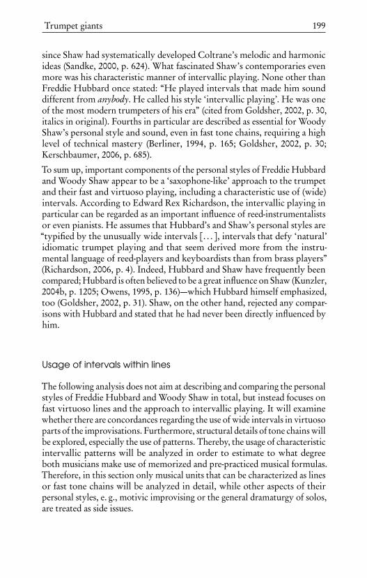
Trumpet giants 199
since Shaw had systematically developed Coltrane’s melodic and harmonicideas (Sandke, 2000, p. 624). What fascinated Shaw’s contemporaries evenmore was his characteristic manner of intervallic playing. None other thanFreddie Hubbard once stated: “He played intervals that made him sounddifferent from anybody. He called his style ‘intervallic playing’. He was oneof the most modern trumpeters of his era” (cited from Goldsher, 2002, p. 30,italics in original). Fourths in particular are described as essential for WoodyShaw’s personal style and sound, even in fast tone chains, requiring a highlevel of technical mastery (Berliner, 1994, p. 165; Goldsher, 2002, p. 30;Kerschbaumer, 2006, p. 685).
To sum up, important components of the personal styles of Freddie Hubbardand Woody Shaw appear to be a ‘saxophone-like’ approach to the trumpetand their fast and virtuoso playing, including a characteristic use of (wide)intervals. According to Edward Rex Richardson, the intervallic playing inparticular can be regarded as an important influence of reed-instrumentalistsor even pianists. He assumes that Hubbard’s and Shaw’s personal styles are“typified by the unusually wide intervals [. . . ], intervals that defy ‘natural’idiomatic trumpet playing and that seem derived more from the instru-mental language of reed-players and keyboardists than from brass players”(Richardson, 2006, p. 4). Indeed, Hubbard and Shaw have frequently beencompared; Hubbard is often believed to be a great influence on Shaw (Kunzler,2004b, p. 1205; Owens, 1995, p. 136)—which Hubbard himself emphasized,too (Goldsher, 2002, p. 31). Shaw, on the other hand, rejected any compar-isons with Hubbard and stated that he had never been directly influenced byhim.
Usage of intervals within lines
The following analysis does not aim at describing and comparing the personalstyles of Freddie Hubbard and Woody Shaw in total, but instead focuses onfast virtuoso lines and the approach to intervallic playing. It will examinewhether there are concordances regarding the use of wide intervals in virtuosoparts of the improvisations. Furthermore, structural details of tone chains willbe explored, especially the use of patterns. Thereby, the usage of characteristicintervallic patterns will be analyzed in order to estimate to what degreeboth musicians make use of memorized and pre-practiced musical formulas.Therefore, in this section only musical units that can be characterized as linesor fast tone chains will be analyzed in detail, while other aspects of theirpersonal styles, e. g., motivic improvising or the general dramaturgy of solos,are treated as side issues.

200 Benjamin Burkhart
Table 1: Percentage of midlevel units in solos by Freddie Hubbard and Woody Shaw.
MLU main type Hubbard Shaw
lick 58.9 48.9line 21.9 22.2melody 10.9 14.7rhythm 6.8 4.9void 0.0 1.1fragment 0.0 1.5expressive 1.0 4.9quote 0.5 0.0theme 0.0 1.9
The Weimar Jazz Database contains six solos by Freddie Hubbard, recordedduring a period from 1960–1966. In the case of Woody Shaw, the databaseencompasses eight solos, recorded in 1977, 1978, and 1987. The improvisa-tional units that shall be explored were chosen with the aid of the midlevelanalysis approach (cf. Chapter Computational melody analysis). In doing so,jazz improvisations are interpreted based on successions of musical unitsbased on various ideas. There are nine main categories for labeling thoseunits: line, lick, melody, theme, rhythm, expressive, quote, fragment, andvoid. Table 1 provides an overview of the percentages of midlevel units inthe solos by Freddie Hubbard and Woody Shaw. In total, 192 midlevel unitswere annotated in the solos by Hubbard, and 266 in the solos by Shaw. Thepercentages of midlevel units labeled as lines are similar for both musicians.Still, there are clear differences regarding the overall percentage of midlevelcategories. Hubbard plays more licks, and he also improvises more rhyth-mically. Shaw, on the other hand, clearly plays more melodies, fragments,and expressive passages, or leaves voids. In general, Woody Shaw’s solos aremore variably structured, since the entropy of midlevel units is 1.45, whereasin Hubbard’s solos it is 1.23 (cf. Chapter Computational melody analysis).A first step for a comparison of the structural details can be undertakenby statistically analyzing the durations, numbers of played tones, and eventdensities of all the lines by Freddie Hubbard and Woody Shaw (Table 2). Theobvious differences concern the median number of tones per line and themedian event density, for which Shaw’s values are clearly higher. Overall,the values for both musicians appear to be comparable. Especially the largerange for duration, number of tones, and event density can be regarded asone obvious concordance in the personal styles of Hubbard and Shaw.
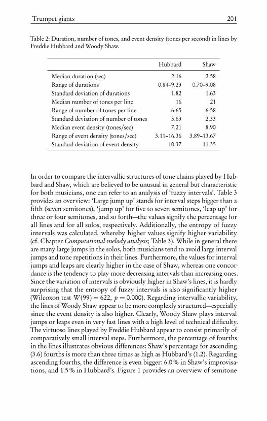
Trumpet giants 201
Table 2: Duration, number of tones, and event density (tones per second) in lines byFreddie Hubbard and Woody Shaw.
Hubbard Shaw
Median duration (sec) 2.16 2.58Range of durations 0.84–9.23 0.70–9.08Standard deviation of durations 1.82 1.63Median number of tones per line 16 21Range of number of tones per line 6-65 6-58Standard deviation of number of tones 3.63 2.33Median event density (tones/sec) 7.21 8.90Range of event density (tones/sec) 3.11–16.36 3.89–13.67Standard deviation of event density 10.37 11.35
In order to compare the intervallic structures of tone chains played by Hub-bard and Shaw, which are believed to be unusual in general but characteristicfor both musicians, one can refer to an analysis of ‘fuzzy intervals’. Table 3provides an overview: ‘Large jump up’ stands for interval steps bigger than afifth (seven semitones), ‘jump up’ for five to seven semitones, ‘leap up’ forthree or four semitones, and so forth—the values signify the percentage forall lines and for all solos, respectively. Additionally, the entropy of fuzzyintervals was calculated, whereby higher values signify higher variability(cf. Chapter Computational melody analysis; Table 3). While in general thereare many large jumps in the solos, both musicians tend to avoid large intervaljumps and tone repetitions in their lines. Furthermore, the values for intervaljumps and leaps are clearly higher in the case of Shaw, whereas one concor-dance is the tendency to play more decreasing intervals than increasing ones.Since the variation of intervals is obviously higher in Shaw’s lines, it is hardlysurprising that the entropy of fuzzy intervals is also significantly higher(Wilcoxon test W (99) = 622, p = 0.000). Regarding intervallic variability,the lines of Woody Shaw appear to be more complexly structured—especiallysince the event density is also higher. Clearly, Woody Shaw plays intervaljumps or leaps even in very fast lines with a high level of technical difficulty.The virtuoso lines played by Freddie Hubbard appear to consist primarily ofcomparatively small interval steps. Furthermore, the percentage of fourthsin the lines illustrates obvious differences: Shaw’s percentage for ascending(3.6) fourths is more than three times as high as Hubbard’s (1.2). Regardingascending fourths, the difference is even bigger: 6.0 % in Shaw’s improvisa-tions, and 1.5 % in Hubbard’s. Figure 1 provides an overview of semitone

202 Benjamin Burkhart
Table 3: Distribution and entropy of fuzzy intervals in solos by Freddie Hubbard andWoody Shaw.
Freddie Hubbard Woody Shawlines (%) solos (%) lines (%) solos (%)
Large jump up 1.0 3.5 0.3 1.6Jump up 2.5 3.7 7.8 8.3Leap up 7.2 8.8 9.0 9.3Step up 27.9 24.6 24.6 23.4Repetition 1.5 7.1 1.2 5.6Step down 46.5 34.6 38.4 31.6Leap down 11.2 12.6 13.7 13.7Jump down 1.8 3.9 4.9 6.2Large jump down 0.4 1.1 0.1 0.3
Entropy (median) 0.42 0.76 0.59 0.72
interval distribution in all lines by Freddie Hubbard and Woody Shaw. SinceWoody Shaw obviously plays wide intervals even in high-speed tone chains,one may ask if he makes use of pre-conceived patterns to meet the technicalchallenge of playing wide intervals in fast lines.
Usage of long patterns
According to musicologist Thomas Owens, patterns play a distinctive rolefor the improvisational language of jazz musicians: “Every mature jazz mu-sician develops a repertory of motives and phrases which he uses in thecourse of his improvisations. His ‘spontaneous’ performances are actuallypre-composed to some extent” (Owens, 1974, p. 17). The improvisations ofFreddie Hubbard and Woody Shaw are assumed to be influenced by modalscales, e. g., “a pentatonic sort of scale” (cited from Berliner, 1994, p. 228).Such assumptions imply clear concordances of their improvisational styles,especially regarding the usage of certain interval patterns.
When searching for recurring formulas in Hubbard’s and Shaw’s solos, therewere various exclusion criteria for the selection of passages that can be definedas patterns. On the one hand, repetitions of single tones, which appear severaltimes in solos by both musicians, were not considered. The same appliesto oscillations of two or more tones. Additionally, since only tone chainswere analyzed and as the aim was to exclude short patterns that might only

Trumpet giants 203
Figure 1: Interval histogram over lines in solos by Freddie Hubbard and Woody Shaw.
be repeated by accident, comparatively long patterns of at least eight tonesoccurring at least twice in at least two different solos were searched for. Itcan be assumed that patterns of at least eight tones that occur in differentimprovisations and in different metrical or harmonic contexts are unlikelyto have been created ‘on the fly’ but are instead practiced and learned inadvance. Since one focus of this chapter is on interval structures, intervalpatterns were taken into consideration—that is, patterns of the same intervals,independent from actual pitches. Searching for patterns meeting the abovementioned criteria results in 77 patterns in Hubbard’s improvisations, and125 in Shaw’s. Most of those patterns are played within different solos, whilepatterns played twice (or more) in only one solo are rather seldom (Table 4).23
In the solos contained in the Weimar Jazz Database, Freddie Hubbard seldomplays patterns longer than eight, and never longer than nine tones occurringin two or more improvisations. Woody Shaw makes use of interval patternsmore extensively than Freddie Hubbard, even though the numbers of patternsoccurring in more than one solo are comparable. However, there are twostriking exceptions: Freddie Hubbard’s solo on “Maiden Voyage” and WoodyShaw’s solo on “In a Capricornian Way”. All patterns that are alike withrespect to the intervallic structure, independent of duration or rhythm, arelisted. Hence, the results must be cross-checked (by ear) in order to check if
23Since mistakes in the transcriptions must be expected, it is just possible that there are evenmore patterns in the solos that cannot be analyzed in this chapter.

204 Benjamin Burkhart
Table 4: Interval patterns in solos by Freddie Hubbard and Woody Shaw.
Performer Solo Interval patterns
Freddie Hubbard 245 0Dolphin Dance 2Down Under 0Maiden Voyage 30Society Red 9Speak No Evil 0All eight solos 77At least two solos 59
Woody Shaw Dat Dere 7If I Were a Bell 9Imagination 8In a Capricornian Way 26Rahsaan’s Run 8Rosewood 6Stepping Stone 4Steve’s Blues 6All eight solos 125At least two solos 72
Note. Only interval patterns counted with at least eight elementsoccurring at least twice.
they sound similar, too. This is of particular relevance in this chapter, sincethe aim is to explore characteristics in fast tone chains. In a first step, onecan refer to the durations of patterns—only comparatively short durationscan refer to lines. Secondly, if durations of two or more listed patterns aresimilar, musical similarities should be checked by ear. When checking the 59interval patterns that can be found in at least two of Hubbard’s solos, it mustbe stated that there are only two results: an ascending line of eight tones heplays both on “Dolphin Dance” (2:21 min, original recording) and “MaidenVoyage”(3:15 min, original recording). That is, Hubbard largely avoids longinterval patterns occurring in two or more solos that sound similar withrespect to duration and rhythm. Additionally, patterns that appear to behighly similar are almost not part of the fast tone chains that are in the focusof this chapter.

Trumpet giants 205
Figure 2: Interval patterns (13 intervals) in solos by Woody Shaw: “In a CapricornianWay” (top) and “Rahsaan’s Run” (bottom). The beams above the staves mark thepatterns, the numbers signify the interval steps in semitones.
Woody Shaw, on the other hand, plays several patterns that are similar ina musical sense within different solos and parts of high tempo tone chains.One striking example is a pattern of 13 intervals occurring in the solos on“In a Capricornian Way” and “Rahsaan’s Run” (Figure 2). Rhythmically, thetwo examples are slightly different, but the patterns are obviously parts ofcomparatively fast tone chains. The durations are 1.15 s (“In a CapricornianWay”), and 1.36 s (“Rahsaan’s Run”). Whereas the patterns mainly consistof small interval steps up to three semitones, Shaw also plays a major third(4) and a fourth (5). Tellingly, not only the intervals but also the pitchesare identical. Another example that illustrates Woody Shaw’s usage of wideintervals in virtuoso lines even better is a twelve-interval-pattern occurring in“In a Capricornian Way” and “Rosewood” (Figure 3). In this case, the durationsare again very similar: 1.21 seconds (“In a Capricornian Way”), and 1.14 s(“Rosewood”). Woody Shaw plays fifths (7), fourths (5), and major thirds(4), which is rather challenging due to the very high tempo. Interestinglyenough, the absolute pitches are transposed by one semi-tone here. Tonally,the first instance is clearly outside, utilizing A major tones over an E[7sus4
chord, whereas in the second instance the pattern neatly aligns with theunderlying Gm9 chord. One further long pattern can be found in the sametwo solos (Figure 4). Shaw avoids wide intervals until the end of the pattern,where he plays two fourths. Again, the absolute pitches are identical here,but the metrical location is shifted by half a beat. Tonally, the first instanceuses tones from the Eb minor scale over an F7sus4 chord, which is slightly off,whereas the second instance fully fits the A[7sus4 chord, with a rather outsideEb minor pickup on beat four of the preceding measure.
As a matter of fact, fourth-steps indeed appear to be an essential characteristicof Shaw’s improvisations, even at very high tempi. The interval patterns oc-
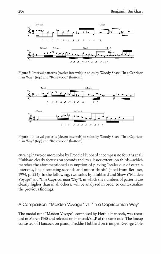
206 Benjamin Burkhart
Figure 3: Interval patterns (twelve intervals) in solos by Woody Shaw: “In a Capricor-nian Way” (top) and “Rosewood” (bottom).
Figure 4: Interval patterns (eleven intervals) in solos by Woody Shaw: “In a Capricor-nian Way” (top) and “Rosewood” (bottom).
curring in two or more solos by Freddie Hubbard encompass no fourths at all.Hubbard clearly focuses on seconds and, to a lesser extent, on thirds—whichmatches the aforementioned assumption of playing “scales out of certainintervals, like alternating seconds and minor thirds” (cited from Berliner,1994, p. 224). In the following, two solos by Hubbard and Shaw (“MaidenVoyage” and “In a Capricornian Way”), in which the numbers of patterns areclearly higher than in all others, will be analyzed in order to contextualizethe previous findings.
A Comparison: “Maiden Voyage” vs. “In a Capricornian Way”
The modal tune “Maiden Voyage”, composed by Herbie Hancock, was recor-ded in March 1965 and released on Hancock’s LP of the same title. The lineupconsisted of Hancock on piano, Freddie Hubbard on trumpet, George Cole-

Trumpet giants 207
Figure 5: Event density (tones per second) over phrases in Freddie Hubbard’s solo on“Maiden Voyage” and Woody Shaw’s solo on “In a Capricornian Way”.
man on tenor saxophone, Ron Carter on bass, and Tony Williams on drums.Hubbard’s solo has been described as “a magnificently creative improvisa-tion”, due to the combination of melodic, rhythmic, and rapid scalar passages(Kernfeld, 1995, p. 150). When listening to the improvisation, the impres-sion of a clearly thought-out dramaturgy and an increasing intensity arises—ranging from fairly cantabile passages at the beginning to virtuoso scalar linesat the end. To illustrate the course of intensity, Figure 5 demonstrates thedevelopment of event density (number of tones per second) per phrase. Theevent density clearly increases over the course of the solo, while decreasingat the end; the values range from 1.31 (phrase 5) to 14.76 (phrase 11).
The high event density results from the fast tone chains that start at 3:48 minin the original recording. The high number of patterns in Hubbard’s im-provisation is due to these lines: Hubbard constantly repeats and furtherdevelops scalar passages. The longest interval pattern encompasses 20 tones,and also consists of shorter, but still comparatively long patterns of 14 and12 tones occurring in other stages of the improvisation. These rapid tonechains, as notated by Barry Kernfeld in his easy-to-read transcription of thesolo (Kernfeld, 1995, pp. 147ff.), only consist of interval steps up to minorthirds. Hubbard seems to play these lines in a very high tempo in order toincrease the improvisation’s intensity at the end of the solo. He does notre-use ideas introduced in other stages of the improvisation or even in other

208 Benjamin Burkhart
Figure 6: Interval patterns (twelve intervals) in Woody Shaw’s solo on “In a Capricor-nian Way”.
solos contained in the Weimar Jazz Database. Additionally, he clearly focuseson small interval steps—pentatonic scales described as characteristic for Hub-bard’s pattern vocabulary (Berliner, 1994, p. 228) cannot be found in theimprovisation on “Maiden Voyage”.
“In a Capricornian Way”, a composition by Woody Shaw, was recorded in1978 and released on the album Stepping Stones. Live At The Village Vanguardin the same year. The following musicians participated in the recording ses-sion: Woody Shaw (cornet), Carter Jefferson (tenor saxophone), Onaje AllanGumbs (piano), Clint Houston (bass), and Victor Lewis (drums). Figure 5illustrates the event density over phrases in Shaw’s solo. The values rangefrom 2.05 to 13.42 tones per second, which is comparable to Hubbard’s im-provisation on “Maiden Voyage”. The dramaturgical increase of intensity isnot as clear as in “Maiden Voyage”, since there are several peaks and a generalzigzag structure.
Besides the patterns occurring in “In a Capricornian Way” as well as in othersolos by Shaw, there are further examples he plays twice in this improvisation,too. One striking example is a twelve-interval-pattern occurring two times(Figure 6). Obviously, Woody Shaw re-uses a pattern he introduced 39 barsearlier. The harmonic and metrical contexts are rather similar, since Shawsimply shifts the starting position of the pattern from the first to the secondbeat of a bar. Additionally, the absolute pitches are the same. Shaw frequentlyre-uses long interval patterns over the course of the solo, which is illustratedin Figure 7.
Pitch patterns as shown above are no exception in Shaw’s improvisations:Altogether, he plays 56 pitch patterns of at least eight tones occurring in twoor more solos. Freddie Hubbard, on the other hand, only plays 19 comparablepatterns. Clearly, Shaw is more apt to long patterns than Hubbard, interval

Trumpet giants 209
Figure 7: Distribution of interval patterns (eight to thirteen intervals) in WoodyShaw’s solo on “In a Capricornian Way”.
Table 5: Pitch patterns in the solos by Freddie Hubbard and Woody Shaw.
Performer Solo Pitch patterns
Freddie Hubbard 245 0Dolphin Dance 0Down Under 0Maiden Voyage 12Society Red 7Speak No Evil 0
Woody Shaw Dat Dere 4If I Were a Bell 4Imagination 6In a Capricornian Way 22Rahsaan’s Run 8Rosewood 4Stepping Stone 4Steve’s Blues 0
Note. Only pitch patterns counted with at least eight elementsoccurring at least twice.

210 Benjamin Burkhart
or pitch patterns alike. This impression can be confirmed when summarizingthe pitch patterns over all solos by both musicians (Table 5).
Summary
When listening to the improvisations by Freddie Hubbard and Woody Shawcontained in the Weimar Jazz Database, some parallels can be found. Asshown above, Hubbard’s and Shaw’s tone chains are comparable to a certaindegree—especially regarding the percentages of lines in relation to othermidlevel units, or concerning the durations and the numbers of tones per line.But when examining structural details, the differences become obvious. Theintervallic structures of Shaw’s tone chains clearly differ from Hubbard’s,since Hubbard rather tends to make use of wide intervals when playingmusical ideas other than lines. On the other hand, Shaw’s focus on fourths,even in high tempos, could clearly be confirmed. Furthermore, and possiblyas a result of the high technical difficulty resulting from his intervallic playing,Woody Shaw seems to refer to a repertory of memorized patterns that ismuch easier to retrace than in the case of Freddie Hubbard.

Michael Brecker’s “I Mean You”
Wolf-Georg Zaddach
Due to his outstanding instrumental skills and enormous workload as arecording and performing artist, Michael Brecker is “widely regarded as themost influential tenor saxophonist since John Coltrane” (Gans, 2017). In fact,his personal style includes bebop and postbop improvisation as well as souland pop music. Therefore, analyzing his solos can be a fruitful approach tohelp understanding the widely shared opinion about Brecker. Brecker (1949–2007), born and raised in the metropolitan area of Philadelphia, alreadyworked with renowned jazz and fusion musicians like Billy Cobham andHorace Silver in his early 20s, and gained wider recognition with the BreckerBrothers, with his brother Randy on the trumpet. After 1980, Brecker mademore than 15 recordings as a leader. Besides these, he went on appearing as asideman on recordings by Chick Corea, Herbie Hancock, John Abercrombieas well as Art Garfunkel or Billy Joel, among others. When Brecker died dueto complications of leukemia in 2007, he had participated on more than 700recordings and won 15 Grammy Awards.
In 1995, Brecker was featured on Infinity with the McCoy Tyner Trio. Here,Brecker once again demonstrates his energetic and creative improvisation abil-ities. Besides a version of John Coltrane’s “Impressions”—for which Breckerwon a Grammy as “Best Jazz Instrumental Solo”—, the album also containsthe jazz standard “I Mean You”. Originally written and first recorded byswing saxophonist Coleman Hawkins in 1946, the tune was rearranged bypianist Thelonious Monk in 1948 to become the ultimate version with anadditional intro that is repeated after the regular form of 32 measures. It isthis historic background of the song which challenges the improviser on adifferent level than, e.g., a modal tune.
When McCoy Tyner starts playing the first A section without bass and drums,he recalls the tune’s origin and connection to the swing and early modern jazz

212 Wolf-Georg Zaddach
era by using techniques of stride piano comping as well as walking bass lines inthe left hand and unison lines in both hands. The band enters for the secondA section and completes the head, including an odd last measure of 2
4 instead of44 that functions as an upbeat to the repetition of the intro section. The tempois a relaxed medium-up swing with about 180 bpm. Brecker starts his soloright after the head and the repeated intro section. During his rather shortsolo, he makes use of several modern jazz improvisation techniques, such asbebop scales, superimposition of chord progressions, symmetric scales suchas the augmented and the half-step/whole-step scale, and constant structures.Yet these contemporary approaches are contrasted as well as interlinked witha rather traditional, early modern jazz style. How he manages to balance outthe jazz tradition with advanced postbop techniques of improvisation duringthat short solo is remarkable, demonstrating Brecker’s class. In the following,I will provide several analytical observations to corroborate this thesis.
The solo
The recording of “I Mean You” on Infinity follows the standard AABA formof 32 measures as can be found in the 557 Standards compilation (p. 159). Thesolo form reads as follows:
A1 F6 F6 D[7 D7 Gm7 C7 F6 Gm7 C7
A2 F6 F6 D[7 D7 Gm7 C7 F6 F6
B1 E[7 E[7 F6 F6 D[7 D[7 G[7 Gm7 C7
A3 F6 F6 D[7 D7 Gm7 C7 F6 F6
Brecker plays two solo choruses. His solo sounds relaxed and bluesy, and yetmodern and contrasting at certain points. When the solo starts, the listenerdetects the restraint of the rhythm section: After the head is played by thecomplete band, McCoy Tyner stops playing. He accompanies Brecker duringthe first chorus only within the B section. Due to this, the A sections ofBrecker’s first chorus are played as a saxophone trio without any chords,whereas the second chorus is fully accompanied by piano, bass, and drums.However, during the first chorus the bass plays out the harmonic progressionrather clearly, as does McCoy Tyner, who renders the underlying chords withoptional tones, fourth chords and bluesy minor third suspensions on majorchords.
Brecker starts his solo in a somehow relaxed feeling with laid-back eighthnotes. Additionally, possibly in reaction to McCoy Tyner’s absence duringthe first two A sections, he plays phrases that span over four measures each (cf.

Michael Brecker’s “I Mean You” 213
A1 A1 A2 A2 B1 B1 A3 A3
A1 A1 A2 A2 B1 B1 A3 A3
2
1
33 37 41 45 49 53 57 61 65
1 5 9 13 17 21 25 29 33
40
50
60
70
80
40
50
60
70
80
Bar number
MID
I Pitc
h
Figure 1: Piano roll of Brecker’s solo. Phrases are alternatingly colored, form partsshaded gray. Pitch is displayed in MIDI pitch (C4 = 60). Top: first chorus, bottom:second chorus.
Figure 1). The beginning of all four phrases is a little delayed and set towardsthe middle of each measure, with the exception of the third phrase (m. 9,see Figure 3 at the end of this chapter). In doing so, Brecker emphasizes theregular structure of the sections and offers the opportunity to hear the rootsof the underlying chords played by the bass at the beginning of each measure.At the same time, that strategy may give Brecker the chance to develop andreact to the playing of the accompanying band. The tonal material outlinesthe somewhat uncommon chord progression of the tune, especially withthe D[7 and the following D7 in the A section. The overall contour of thephrases is mostly descending. In combination with the laid-back phrasing, herecalls the motion of the theme of the A section and demonstrates a relaxedattitude. As I will show later on in detail, this is also supported by certaintonal choices.
During the second half of the B section, Brecker begins to play lines consistingof sixteenth notes. During the third A section, he seems to start mixing therelaxed feeling of the first half of the chorus and the intensity of the B sectionin terms of speed. The second chorus becomes more intense in terms ofdramaturgy and speed, while the peak is reached in the last A section, right atthe end of the solo. Overall, Brecker emphasizes a heavy swing feeling with

214 Wolf-Georg Zaddach
a swing ratio of 1.77:1 on average, and occasionally almost triplet eighthswith a ratio of 2:1. Other solos by Brecker in the Weimar Jazz Databasedemonstrate similar ratios in tunes with a similar, slightly slower mid-tempo(“Midnight Voyage”, 126 bpm, with 1.7:1 and “Naked Soul”, 92.4 bpm, with1.8:1) as well as rather straight eighths such as in “Peep” (320 bpm) and “CabinFever” (300 bpm). This seems to depend on the overall tempo of the tune, seeFigure 2.
Harmonic treatment, phrase structure and motifs
Over the first two A sections, Brecker plays phrases of four measures lengthwhich start delayed in the middle of each measure (see the full transcriptionbased on the Weimar Jazz Database at the end of this chapter). The solobegins with an accent on beat three of the first measure that repeats theunderlying root and tonic, as if he were shouting out “You”, possibly derivedfrom the three-tone motif of the theme whose rhythm fits the phrase “I MeanYou”. What follows is a descending line using the F major scale referring tothe descending motif of the theme. Since the line expands onto four mea-sures, Brecker needs to adjust and transform the line harmonically to the D[7
chord in m. 3, while he is still on a descending move. Here, Brecker plays adescending G7]5 arpeggio as the tritone substitution to the underlying D[7.
During that first phrase, Brecker offers an interesting strategy to connect thesomewhat unusual progression of F6 | F6 | D[7 | D7. While the first measuresare purely inside F major, the following D[7 and D7 create an interestingtension due to their chromatic connection as well as an implied conversion ofa dominant cycle or cycle of fifth to a cycle of fourths, if the D[7 is interpretedas the tritone substitution of G7. How does Brecker handle this progressionexactly? Due to a slight and chromatic adjustment of the F on the last beatof m. 3 to an E on the first beat of m. 4, he displays the harmonic shiftmoving from the major third of the D[7 to the ninth of the D7. At the sametime, he repeats the B natural from m. 3, the minor seventh of D[7, againover the D7. If one interprets the D7 in F and therefore as the secondarydominant (V7/II) to the following Gm7, the B[ as a flatted 13th would be therequired pitch for the D7. But on the contrary, in m. 4 Brecker uses a D majorpentatonic with the B natural on a strong beat. Nonetheless, in playing thenatural B over the D7, Brecker creates a specific connection between bothmeasures in stressing the meaning and relevance of this prominent chromaticprogression that is typical for the music of Thelonious Monk, for examplein tunes like “Well You Needn’t” or “Epistrophy”. Brecker keeps using theB natural instead of the B[ over the D7 for the rest of solo, but contextualizes

Michael Brecker’s “I Mean You” 215
Delta City Blues (282 bpm)
Song for Bilbao (184 bpm)
Cabin Fever (300 bpm)
Peep (320 bpm)
Confirmation (209 bpm)
Nothing Personal (244 bpm)
I Mean You (180 bpm)
Midnight Voyage (126 bpm)
Naked Soul (92 bpm)
1 2 3
Swing Ratios
Figure 2: Box plot of swing ratios of Michael Brecker solos in the Weimar Jazz Da-tabase. Only swing ratios between 1:1 and 4:1 are kept. “I Mean You” has a medianswing ratio of 1.92:1 and forms together with “Naked Soul” and “Midnight Voyage”a group of ‘heavy swinging’ solos.
it differently, e.g., as part of a A minor pentatonic implication in m. 28 or anaugmented E7 in m. 44. Additionally, this approach in the first four measuresallows Brecker to divide the A sections into two harmonically consistent andcoherent phrases of four measures with a harmonically rather interestingfirst part and a traditional II–V–I-cadence in the second part.
In the first B section, Brecker already deviates from a regular four-measurephrasing. He enters and leaves the B section by connecting with the A sectionsthrough expansions of the ongoing phrases so that they each end in the nextsection (cf. Figure 1). Even though he kind of jumps into it, this first B sectionfollows the overall phrase division of four measures. Nevertheless, he marksthe beginning of the B section with a new motif: From the descending F bebopscale in m. 16, he develops a motif that is striking due to its distinctiverhythm and tonal material of B[minor pentatonic over the E[7. The B[minorpentatonic creates a sus4 sound over the underlying E[7, but is also a coherentconsequence of the descending F bebop dominant scale that Brecker playsin the preceding measure. Brecker transforms this idea into a leap sequenceof ascending fourths in mm. 19 and 20, suggesting an F7sus4 that is resolvedinto a F7. At this point, the first four measures of the B section are completedfollowing the previous structure and yet varying it with distinctive motifs

216 Wolf-Georg Zaddach
and breaks in between. The second half of the B section offers the first fastplayed line of mostly sixteenth notes. This phrase, which peaks in the firstmeasure of the following A section with a high F, makes use of superimposedscales. The last A section is less clearly structured, though Brecker outlines theII–V–I progression and an additional turn-around with a superimposed chordprogression that will be discussed later. The function of that superimpositionis to clearly mark the end of the first chorus with a first climax.
The second chorus follows the rather loose structuring introduced in thesecond half of the first chorus. This allows Brecker to develop complexphrases with features of postbop improvisation such as four-tone patterns incombination with advanced harmonic or melodic ideas. Nevertheless, duringthe first two A sections of the second chorus, Brecker still seems to rely onthe middle of the section as a focal point, releasing the tension mainly interms of speed, but also harmonically.
In the B section, Brecker does not follow the regular phrase division anymore,but instead indicates the section again through motivic development. In m. 54,he plays in a descending motion the flatted fifth, the fourth and the majorthird of the underlying D[7, which he repeats transposed and adjusted to theunderlying C7 in m. 56. Both are connected and seem to be a spontaneousinvention. In doing so, he creates a guide tone line that descends chromaticallyin m. 54 from a B[ to an E (though the A[ is missing in m. 54) and is theninterrupted by a measure and yet connected throughout the repetition of theG[7 and the chromatic descending contour. The interrupting m. 55 stands outdue to its harmonic content as well: Over the underlying G[7, one can hear aclear Gm7 arpeggio, with the minor third and root at the end of the phrase.One could interpret this in two different ways: a) Brecker makes use of side-stepping as a typical technique for playing outside (see below); b) Breckerapproaches these last two measures with a horizontal displacement in whichhe anticipates the Gm7 chord of the first half of the last measure having afull measure to fill with the C7. At the same time, easily perceivable for thelistener, the descending motif sounds bluesy and sly, which is an importantgeneral feature of Brecker’s solo. The last A section is the highlight of thesolo and contains mainly lines of sixteenth notes. Concerning the structuringof the phrases, it is the most outstanding section of the whole solo, makinguse of advanced techniques.
The usage of blues and bebop scales
During his relatively short solo, Brecker clearly makes references to thestylistic context of the piece, the late swing era as well as the bebop era as

Michael Brecker’s “I Mean You” 217
personified by the composers of the piece, Hawkins and Monk. Breckeruses several distinct techniques that echo this origin of modern jazz in par-ticular: He re-harmonizes the tonic into a dominant seventh chord, usesblues and bebop scales, and quotes Charlie Parker. Brecker already uses there-harmonization of the tonic F6 in the first measure of the A2 of the firstchorus (mm. 9 and 10). Here, he clearly plays the E[ as the dominant seventhover two measures, the first on the strong beat three of m. 9. He does thesame over the last two measures of the same section and the two measures ofF in the first B section (mm. 19 and 20). For rest of the solo, Brecker avoidsplaying any sevenths over the F tonic with two exceptions in mm. 25 and26 right after the first B section and in m. 52 in the second B section. Eventhough he does not repeat the minor seventh, the strong implication of thebluesy tonic has already been established by Brecker and picked up by theband. Interestingly, bassist Avery Sharps reacts already immediately to thefirst E[ in m. 9 on beat three played by Brecker and plays an E[ on beat four,leading into an F on the next beat followed by a descending chromatic linetowards D, which can be understood as a typical F bebop dominant scale. Atthe end of the section, when Brecker again plays a F7, Sharps incorporatesthe E[ again in a bass line rising from the root to the fifth with the minor andmajor third and adding the E[ and F on top. In the B section, both Sharpsand McCoy Tyner emphasize the F7 as well. McCoy Tyner has obviouslybeen listening during the previous A sections and plays the F7, with theadditional blues influenced grace note of the minor third, simultaneouslywith Brecker’s E[ on beat three. In m. 25 in the A3 section, when Breckerswitches back to the original F major seventh, Sharps outlines tones of theF major pentatonic while avoiding any sevenths. During m. 31 at the endof the section, he plays F–E[–D–A[, which amounts to an F7 and D7, re-spectively, the substitution A[7, which easily leads to the following Gm7
and C7 to complete the turn-around. During the following F6 chords, whenBrecker tends to avoid the seventh, the band seems to be still aware that hecould repeat the blues influenced re-harmonization: In m. 33, right at thebeginning of the second chorus, Sharps uses the E[ again as a passing tone; inm. 47 before the second B section, he clearly plays an F7 in the first measurewith repeated insistence (F–F–E[–E[) while Brecker plays a fast descendingline that implies A7 with the additional blues interval of the flatted fifth—apossible indication of the coming E[7 as a tritone substitution. McCoy Tynerkeeps the re-harmonization in mind as well, indicated by a bluesy F in m. 45with the grace note of a minor third.
Blues and bebop scales are another feature that Brecker uses during his solo.According to Levine, a blues influenced scale is one of the “oldest, most basicmelodic material” that has been played on the blues (Levine, 1995, p. 202ff.).
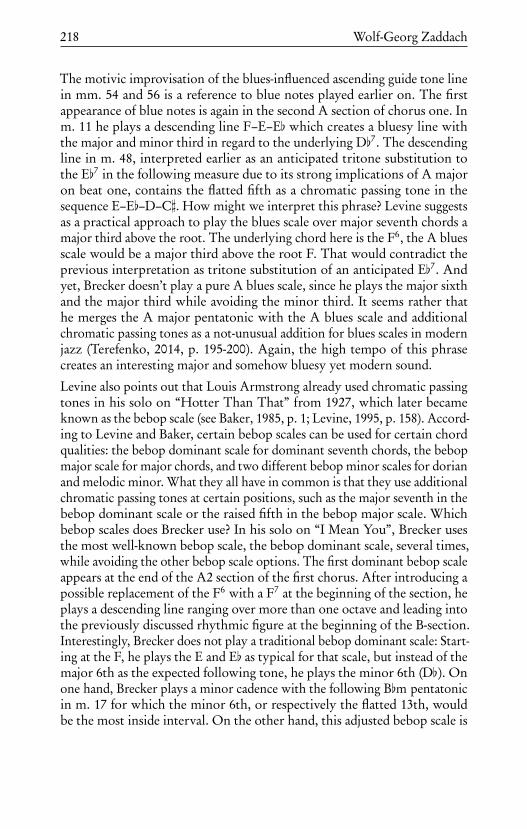
218 Wolf-Georg Zaddach
The motivic improvisation of the blues-influenced ascending guide tone linein mm. 54 and 56 is a reference to blue notes played earlier on. The firstappearance of blue notes is again in the second A section of chorus one. Inm. 11 he plays a descending line F–E–E[ which creates a bluesy line withthe major and minor third in regard to the underlying D[7. The descendingline in m. 48, interpreted earlier as an anticipated tritone substitution tothe E[7 in the following measure due to its strong implications of A majoron beat one, contains the flatted fifth as a chromatic passing tone in thesequence E–E[–D–C]. How might we interpret this phrase? Levine suggestsas a practical approach to play the blues scale over major seventh chords amajor third above the root. The underlying chord here is the F6, the A bluesscale would be a major third above the root F. That would contradict theprevious interpretation as tritone substitution of an anticipated E[7. Andyet, Brecker doesn’t play a pure A blues scale, since he plays the major sixthand the major third while avoiding the minor third. It seems rather thathe merges the A major pentatonic with the A blues scale and additionalchromatic passing tones as a not-unusual addition for blues scales in modernjazz (Terefenko, 2014, p. 195-200). Again, the high tempo of this phrasecreates an interesting major and somehow bluesy yet modern sound.
Levine also points out that Louis Armstrong already used chromatic passingtones in his solo on “Hotter Than That” from 1927, which later becameknown as the bebop scale (see Baker, 1985, p. 1; Levine, 1995, p. 158). Accord-ing to Levine and Baker, certain bebop scales can be used for certain chordqualities: the bebop dominant scale for dominant seventh chords, the bebopmajor scale for major chords, and two different bebop minor scales for dorianand melodic minor. What they all have in common is that they use additionalchromatic passing tones at certain positions, such as the major seventh in thebebop dominant scale or the raised fifth in the bebop major scale. Whichbebop scales does Brecker use? In his solo on “I Mean You”, Brecker usesthe most well-known bebop scale, the bebop dominant scale, several times,while avoiding the other bebop scale options. The first dominant bebop scaleappears at the end of the A2 section of the first chorus. After introducing apossible replacement of the F6 with a F7 at the beginning of the section, heplays a descending line ranging over more than one octave and leading intothe previously discussed rhythmic figure at the beginning of the B-section.Interestingly, Brecker does not play a traditional bebop dominant scale: Start-ing at the F, he plays the E and E[ as typical for that scale, but instead of themajor 6th as the expected following tone, he plays the minor 6th (D[). Onone hand, Brecker plays a minor cadence with the following B[m pentatonicin m. 17 for which the minor 6th, or respectively the flatted 13th, wouldbe the most inside interval. On the other hand, this adjusted bebop scale is

Michael Brecker’s “I Mean You” 219
discussed in jazz theory as one of the ‘altered bebop scales’, in this case theF bebop dominant [13 scale (Terefenko, 2014, p. 205). Brecker even mixesboth dominant scales, with the F bebop dominant scale and the major sixthduring the second half of m. 16, leading into a B[minor triad. The next bebopdominant scale appears during the A3 section of the first chorus over theD[7 in m. 27. Here, Brecker plays the characteristic major and minor seventhand the major sixth. What is new at this point is that he alters the meaningof the scale by altering the positions of the intervals. While the appearanceof the bebop scale is often explained by ensuring that the important chordintervals (root, third, fifth and seventh) fall on the strong beats by addingchromatic passing tones, Brecker reverses that logic at this point. Startingwith the root D[ on an offbeat, he places the major seventh as one of thechromatic passing tones on a strong beat. With that phrase, which spansroughly two beats, he augments the D[7 over the bar line into the followingD7, which therefore sounds like a moment of outside playing, describableas side-slipping (Liebman, 2006, p. 55–58). The last appearance of the bebopdominant scale is rather hidden and embedded in a phrase that spans twoand a half measures right at the end of the solo (mm. 62–64). Embedded in asuperimposed chord progression, Brecker plays the E[ bebop dominant scalein m. 63 on beat three and the C bebop dominant scale on beat four, merginga modern superimposition with a rather traditional bebop phrasing.
Another connection to the bebop era can be found in a perhaps rather uncon-scious quote from well-established Parker formulas (Owens, 1974). Again, itis the A2 section of the first chorus that offers such a lick. In m. 13, Breckerstarts a convincingly bebop-ish phrase which ends with the usage of theF bebop dominant scale discussed above. After a rather long break of two-and-a-half beats, he plays an ascending B[major triad initiated by a chromaticapproach from the leading tone below. Thomas Owens identifies this phrase—in the exact rhythm with a triplet—as a typical formula often played byCharlie Parker over a B[maj chord (Owens, 1974, p.87-93). It is very likelythat Brecker plays that formula here rather unconsciously since he probablypracticed Parker solos a lot. Also, even if the pause before that formula givesBrecker some time to consider such a quote, he may have had somethingmore “traditional” or “bebop-ish” in mind, rather than planning to play thatexact formula.
Superimposed scales and virtual chord progressions
The superimposition of an improvised chord progression over the composedchord progression has, ever since its popularization by John Coltrane, been
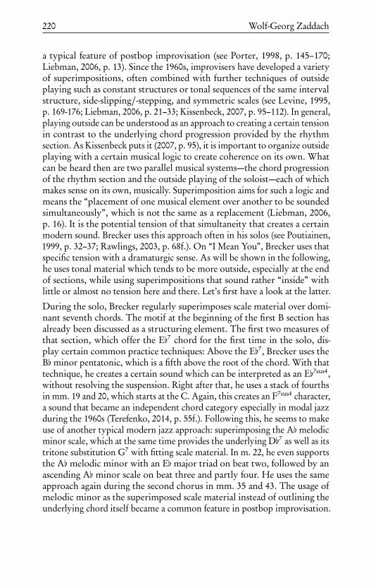
220 Wolf-Georg Zaddach
a typical feature of postbop improvisation (see Porter, 1998, p. 145–170;Liebman, 2006, p. 13). Since the 1960s, improvisers have developed a varietyof superimpositions, often combined with further techniques of outsideplaying such as constant structures or tonal sequences of the same intervalstructure, side-slipping/-stepping, and symmetric scales (see Levine, 1995,p. 169-176; Liebman, 2006, p. 21–33; Kissenbeck, 2007, p. 95–112). In general,playing outside can be understood as an approach to creating a certain tensionin contrast to the underlying chord progression provided by the rhythmsection. As Kissenbeck puts it (2007, p. 95), it is important to organize outsideplaying with a certain musical logic to create coherence on its own. Whatcan be heard then are two parallel musical systems—the chord progressionof the rhythm section and the outside playing of the soloist—each of whichmakes sense on its own, musically. Superimposition aims for such a logic andmeans the “placement of one musical element over another to be soundedsimultaneously”, which is not the same as a replacement (Liebman, 2006,p. 16). It is the potential tension of that simultaneity that creates a certainmodern sound. Brecker uses this approach often in his solos (see Poutiainen,1999, p. 32–37; Rawlings, 2003, p. 68f.). On “I Mean You”, Brecker uses thatspecific tension with a dramaturgic sense. As will be shown in the following,he uses tonal material which tends to be more outside, especially at the endof sections, while using superimpositions that sound rather “inside” withlittle or almost no tension here and there. Let’s first have a look at the latter.
During the solo, Brecker regularly superimposes scale material over domi-nant seventh chords. The motif at the beginning of the first B section hasalready been discussed as a structuring element. The first two measures ofthat section, which offer the E[7 chord for the first time in the solo, dis-play certain common practice techniques: Above the E[7, Brecker uses theB[minor pentatonic, which is a fifth above the root of the chord. With thattechnique, he creates a certain sound which can be interpreted as an E[7sus4,without resolving the suspension. Right after that, he uses a stack of fourthsin mm. 19 and 20, which starts at the C. Again, this creates an F7sus4 character,a sound that became an independent chord category especially in modal jazzduring the 1960s (Terefenko, 2014, p. 55f.). Following this, he seems to makeuse of another typical modern jazz approach: superimposing the A[melodicminor scale, which at the same time provides the underlying D[7 as well as itstritone substitution G7 with fitting scale material. In m. 22, he even supportsthe A[ melodic minor with an E[ major triad on beat two, followed by anascending A[ minor scale on beat three and partly four. He uses the sameapproach again during the second chorus in mm. 35 and 43. The usage ofmelodic minor as the superimposed scale material instead of outlining theunderlying chord itself became a common feature in postbop improvisation.

Michael Brecker’s “I Mean You” 221
He continues with superimpositions till the end of the first B section. In m. 23,he superimposes four independent four-tone patterns over the G[7 whichimply a chord sequence that could be interpreted as the following: Gm7, C7,B[, D7. The Gm7 and C7 can be understood as a II–V tritone substitution tothe underlying G[7, while the B[ is a major third above the G[. The D7 leadsto the following Gm7 in m. 24. Here, Brecker continues to color the C7 withD[melodic minor, which gives the C7 an altered sound.
The next superimposition at the end of the first chorus offers the usageof another feature of outside playing. The lines in mm. 31 and 32 at theend of the chorus could imply a turnaround with an additional D7, Gm7
and C7 as a common practice in jazz. During that turnaround, indicatedby the bass, Brecker plays the following sequence: an F major triad in anascending motion, an F] major triad in a descending motion, an E majortriad in an ascending motion and again a descending F]major triad leadingto the tonic F at the beginning of the second chorus. Each arpeggio consistsof four notes and fills up the space of two beats—the same way a turnarounddoes. The triad structure and regular contour of the phrases creates its ownlogic and consistency. Yet Brecker does not play a complete turnaround ofI–VI–II–V but rather expands resp. augments the dominant C7 over mm. 31and 32. In doing so, he is able to play a longer line that has a dominantfunction. Following this reading, the F] major triad can be understood asa tritone substitution to the C7. The E major triad then could be a side-slipping from the tonic F. The F] again repeats the dominant function of thatsuperimposition.
However, the usage of the E major triad could also be interpreted as a deriva-tion of the augmented scale. The augmented scale can be understood as aninterlocking combination of two augmented triads which are a minor thirdapart from each other (Weiskopf & Ricker, 1993). This creates a certain scalesequence of minor thirds and minor seconds. In C, the scale consists of anaugmented C triad and an augmented E[ triad and builds the following scale:C–E[–E–G–G]–B. It is likely that Brecker uses the C altered and C augmentedscale in an interlocking fashion here to create this sequence of triads. Whilethe tritone substitution of the C7 can easily be derived from the C scale (orlikewise be understood as alterations of the upper structure), the E majortriad is provided in the C augmented scale. This specific usage of the aug-mented scale on dominant chords—a triad (with or without the raised fifthand an additional major seventh) built a major third above the root—hadoften been identified in Brecker’s playing (see Weiskopf & Ricker, 1993, p. 7;Rawlings, 2003, p. 121, 124, 127, 163). He seems to use that approach onthe second chorus in m. 44 as well, superimposing an E augmented triadderived from the C augmented scale over the underlying D7. Only the D
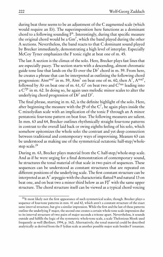
222 Wolf-Georg Zaddach
during beat three seems to be an adjustment of the C augmented scale (whichwould require an E[). The superimposition here functions as a dominantchord to a following sounding F6. Interestingly, during that specific measurethe original chord would be a Gm7, which the band played during the otherA sections. Nevertheless, the band reacts to that C dominant sound playedby Brecker immediately, demonstrating a high level of interplay. EspeciallyMcCoy Tyner emphasizes the F tonic right at beat one of m. 45.
The last A section is the climax of the solo. Here, Brecker plays fast lines thatare especially pacey. The section starts with a descending, almost chromaticguide tone line that lands on the E[ over the D[7 chord in m. 59. From here,he creates a phrase that can be interpreted as outlining the following chordprogression: A[mmaj7 in m. 59, A[m7 on beat one of m. 60, then A7, Amaj7,followed by A[ on beat one of m. 61, G7 on beat two and C7sus leading intoa C7]9 in m. 62. In doing so, he again uses melodic minor scales to alter theunderlying chord progression of D[7 and D7.
The final phrase, starting in m. 62, is the definite highlight of the solo. Here,after beginning the measure with the ]9 of the C7, he again plays inside theC mixolydian scale with an implication of the tonic F through an A minorpentatonic four-tone pattern on beat four. The following measures are salient.In mm. 63 and 64, Brecker outlines rhythmically straight four-tone patternsin contrast to the overall laid back or swing eighths feeling of his solo, whichsomehow epitomizes the whole solo: the contrast and yet deep connectionbetween traditional and contemporary ways of improvising. Measure 63 canbe understood as making use of the symmetrical octatonic half-step/whole-step scale.24
During m. 63, Brecker plays material from the C half-step/whole-step scale.And as if he were urging for a final demonstration of contemporary sound,he structures the tonal material of that scale in two pairs of sequences. Thesesequences can be understood as constant structures that are repeated ondifferent positions of the underlying scale. The first constant structure can beinterpreted as an A7 arpeggio with the characteristic flatted 9 and natural 13 onbeat one, and on beat two a minor third below as an F]7 with the same upperstructure. The chord structure itself can be viewed as a typical chord voicing
24It most likely not the first appearance of such symmetrical scales, though. Brecker plays asequence of four-tone patterns in mm. 41 and 42, which aren’t a constant structure of the exactsame interval structure, but give a similar impression. While the first and the last of these patternsoutline the underlying F major, the second one creates a certain whole tone scale impression dueto its interval structure of two pairs of major seconds a tritone apart. Nevertheless, it soundsoutside and fulfills the logic of the symmetric whole-tone scale, a scale Thelonious Monk usedfrequently as well (Berliner, 1994, p. 162). Alternatively, the tonal material could be describedanalytically as derived from the F lydian scale as another possible major scale besides F ionanian.
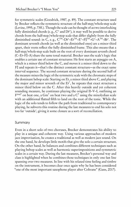
Michael Brecker’s “I Mean You” 223
for symmetric scales (Goodrick, 1987, p. 89). The constant structure usedby Brecker reflects the symmetric structure of the half-step/whole-step scale(Levine, 1995, p. 73ff.). Though the scale can be thought of as two interlockingfully diminished chords (e. g., C and D[), it may well be possible to derivechords from the half-step/whole-step scale that differ slightly from the fullydiminished sound: in C, e. g., C7[9–D[–E[7[9–E–F]7[9–G–A7[9–B[. Thedominant seventh chords (as well as the diminished ones) are a minor thirdapart, their roots reflect the fully diminished frame. This also means that ahalf-step/whole-step scale built on the root of every dominant seventh chord(C–E[–F]–A) share the same tonal material. Brecker uses the scale’s logic thatenables a certain use of constant structures: He first starts an arpeggio on A,which is a minor third below the C, and moves it a minor third down to theF] and repeats it—that’s the distinct constant structure—as the exact sameinterval sequence. The second constant structure during the second half ofthe measure mixes the logic of the symmetric scale with the chromatic steps ofthe dominant bebop scale: Starting on E[, a minor third above C, and playingthe major and minor seventh of the E[7, he repeats that exact structure aminor third below on the C. After this heavily outside and yet coherentsounding measure, he continues playing the original II–V–I, outlining anFmaj7 on beat one, a Gm7 on beat two and a C7 using the mixolydian scalewith an additional flatted fifth to land on the root of the tonic. While thelogic of the solo tends to follow the path from traditional to contemporaryplaying, he subverts this routine during the last measures to end his solo nottoo far ‘outside’, giving it some closure as a sort of reconciliation.
Summary
Even in a short solo of two choruses, Brecker demonstrates his ability toplay in a unique and coherent way. Using various approaches of modernjazz improvisation, he creates a traditional as well as modern jazz sound. Onthe one hand, he develops little motifs that give the solo a certain structure.On the other hand, he balances and combines different techniques such asplaying bebop scales as well as harmonic superimpositions and symmetricscales in a certain way. During the last measures, Brecker’s personal way andclass is highlighted when he combines those techniques in only one fast linespanning over two measures. In line with his relaxed time feeling and timbreon the instrument, it becomes clear once again why he has been considered“one of the most important saxophone player after Coltrane” (Gans, 2017).

224 Wolf-Georg Zaddach
I Mean You
Michael Brecker
í D í7 6
63
í F6F
6
8
í 441
Ì = 180
C7
D7
í
4
8
í G–7
í C
7F6
3
í F6 7
8
í G–7
í í D í7 3
í í D7 í
8
10
F6
3
íG–7
í
13
8
í C
7
í Eí7í í
333
33
í í16
8
í í
í í D í7
3 3
íí í8
F6
19 í í
í 3
í í íí8
22 Gí7 íí
G–7 íí íí 3563
C7
í
8
24
F6
íD í7 íí
6
í D7í í í
8
26 í
F6 í
3333
í í C7í
8
29 G–
7
2 6
3
í í
8
32 í í í
Figure 3: Full transcription of Michael Brecker’s solo, based on the digital transcriptionof the Weimar Jazz Database.

Michael Brecker’s “I Mean You” 225
í D í7
í 3
3 33
íí í í8
íG–
7
35
í D7
C
7
G–73
3
F6 í
38 í8
C7 í
F6
66
8
í41
í 6 6
36
í í
8
í
D í7
43 í D7
í í
F6
6333
G–7í
8
45 F
6 í C
7
Eí7
í í 66
5
í í í
8
48
í íí
33
66
íí íí
8
50
F6
Gí7
í í
3
533
í í 53
8
í Dí7
í íí
G–7 íí í
33
íí í8
56 C7
F6
í íD7íí D í7í
6
6
í í8
59
í
C7
6
3 5 6
í í8
61 íG–
7
í
C7
F6
3
F6
í í í8
63 í í G–
7
í í
Figure 3: (Continued.)


Right into the heart. Branford Marsalis andthe blues “Housed from Edward”
Wolf-Georg Zaddach
Branford Marsalis, saxophonist and member of the Marsalis family, the “FirstFamily of Jazz” (Raz, 2012), was born in 1960 and raised in Louisiana. Whilehis younger brother Wynton Marsalis developed a widely-known advocacyof jazz heritage during the 1980s, Branford followed his own path. Growingup playing in rhythm and blues bands and listening to contemporary funkand pop music, he started digging deeper into jazz rather late, while studyingjazz saxophone at the Berklee College of Music in Boston from 1979 and 1981.Nonetheless, he quickly became one of the most renowned saxophonists ofhis generation. His employers during the 1980s, such as Art Blakey or MilesDavis, were important influences on his development as a jazz musicianas well as on his career. In 1985, the Chicago Tribune called him “a jazzstar of the brightest magnitude”, referring to a quote by Miles Davis, whosupposedly called him the “greatest saxophonist since Coltrane” (Brogan,1985). During that year, Marsalis also started working for Sting, the formerThe Police member, and experienced the glamorous but also—in his ownwords—“gross” world of pop music business (Brogan 1985). While at thattime Wynton criticized Branford for this step as selling out his jazz heritage(Polkow, 1989), Branford remembers it as an important learning progress:
That was one of the things about playing with Sting that wasvery helpful for me. Because I used to play these long ramblingsolos with a lot of space in them and just really didn’t know howto start and finish solos when I was playing in Wynton’s band.And then suddenly I had 90-second solos for a year and a half.And when you have that kind of discipline, where you have toget to it and get out, when I came back to jazz, my solos had alot more intensity and a lot less overthinking (Milkowski, 2012).

228 Wolf-Georg Zaddach
Just a few years after working for Sting, he summarizes that he especiallylearned “aggressive playing” and judged his own playing in the band of hisbrother Wynton during the first half of the 1980s as being “far too tentative”.After his pop experience, when he started playing a lot more jazz again, itfelt to him that he had “a lot of fervor and it was really fresh” (Polkow, 1989).Besides his encounters with pop music, he also recorded classical music byDebussy, Stravinsky and others for the album Romances for Saxophone (1986).Here, he gained a different sense for melody, and the “discipline to play withsimplicity” (Milkowski, 2012). When Marsalis recorded Trio Jeepy in 1988,his sixth album as a leader, he surely could rely on those different experiencesin modern jazz, pop, and classical music.
Trio Jeepy is a trio recording with bass and drums exclusively, and was recordedin New York City. Marsalis chose Milt Hinton (1910–2000) and Delbert Felix(*1958) for bass and Jeff Watts (*1960) for drums. The saxophone trio settingwithout a harmony instrument is a rather modern approach in jazz, called‘strolling’. After Sonny Rollins’s Way Out West (1957), one of the first full-length recordings with that specific setup, it became a frequently used format,especially by the 1960s avant-garde (e. g., Ornette Coleman, Albert Ayler).Marsalis had adopted the strolling approach several times on recordingsbefore, e. g., on the first track of his first solo release Scenes in the City (1984),but had not yet used it for a complete recording. The title list consists mainlyof standards and compositions spanning from the Great American Songbookera to the 1960s, as well as three original compositions by the band. In oneof his previous albums, Renaissance from 1987, he followed a similar mixedapproach, yet the standards there are played rather in a contemporary postbopstyle, while Trio Jeepy has a somehow traditional sound. This is mostly dueto Hinton’s bass playing but also to certain improvising strategies of Marsalis,as will be shown later.
Apparently, Trio Jeepy partly gives the impression of a recorded live concert(though without an audience) or even a rehearsal recording. As Scott Yanowstates, the performances seemed to happen “quite spontaneous[ly]”; it seemsthat the band “had a lot of fun” (Yanow, 2017). False starts and discussionswere left, which was not completely unheard of before in Marsalis’s releases.The short conversations give interesting insights into the band’s social in-teractions, especially between the jazz veteran Hinton and the 27-year-oldMarsalis. The false start of “Three Little Words” (track 3) is one such example.Here, Hinton throws a harsh and yet demanding “You gotta play it, man”at Marsalis (0:13-0:20 min), forcing him to concentrate and start over in aconvincing fashion. This straight-up and demanding mode of communicationwasn’t new to Marsalis at all, it was part of his socio-cultural background: “Igrew up in the South, in New Orleans, where guys torture you all the time

Branford Marsalis and the blues “Housed from Edward” 229
[. . . ]. When you were lousy at something, they told you you were lousy,and they told you how to fix it,” recalls Marsalis, talking about the similarway Art Blakey used to speak to him (Raz, 2012). Pianist and singer HarryConnick Jr. (*1967), a student of Branford’s father Ellis Marsalis in NewOrleans, remembers playing with the Marsalis brothers: “Those guys wereharsh, man! They would verbally cut me down. [. . . ] They would beat youup emotionally. At the time it was tear-inducing” (Panken, 2016). In a recentinterview, Marsalis admits that music students nowadays judge this demand-ing and hands-on mentality as a rather “hostile environment” (Milkowski,2012).
Two of the originals on Trio Jeepy are blues tunes, which is remarkable inso-far as Marsalis’s originals on his previous albums were exclusively postbopcompositions at its best. Turning to the blues might be related to an event inthe mid 80s, when Marsalis was accused by Dizzy Gillespie, with whom heworked at that time, that “he didn’t hear any blues” in his playing (Goodwin,2015). Marsalis admits that his main goal during the first half of the ‘80s was tosound like Coltrane and somewhat modern. Until Trio Jeepy, he had recordedtraditional and blues songs only with Wynton’s band and occasionally as aleader. The blues tunes on Trio Jeepy sound especially old-fashioned in a waythat Marsalis hadn’t released on a solo recording before. Marsalis’s first soloof the blues “Housed from Edward” will be in the focus of the analysis in thefollowing.
“Housed from Edward”—in the safe house of blues?
“Housed from Edward”, the first track of the album, is a blues in F and listedas an original composition by Marsalis. The almost nine-and-a-half-minuterecording is in a relaxed time feel (approx. 127 bpm). Marsalis plays one longerand one short solo; in between are solo choruses by Milt Hinton. The songstarts with Hinton and Marsalis as a duo. At first, Hinton accompanies in ahalf-time feel with half notes outlining the blues progression. Watts entersat the second chorus, and the band plays another two theme choruses in atypical swing 4
4-feeling with walking bass, before Marsalis starts his first soloof 10 choruses. During those first three theme choruses, Marsalis plays ahead-like melody which places dotted half notes on the second beat of everymeasure (Figure 1). The tones mainly emphasize the root, third or fifth ofthe underlying chord progression outlined by the bass. Most of the tones arethe length of half notes—during the first twelve measures there are no fastertones. The rhythmic placement outlines the downbeats, with an emphasis onthe second beat during the first chorus. The first and second repetitions vary

230 Wolf-Georg Zaddach
Figure 1: The theme of “Housed from Edward” as played for the first time, before thesolo starts.
the placement with onsets on beat one. However, due to Marsalis’s variationsand embellishments it sounds improvised rather than composed.
Watts offers a consistent swing drumming that emphasizes beats two andfour of every measure, while reacting to Marsalis’s solo with fills. Hinton’slines clearly emphasize the jazz blues chord progression without employingadvanced (postbop) strategies such as covering up the underlying chord orharmonic progression, e. g., playing the second of the underlying chordon beat one. Furthermore, he plays constant quarter notes with only fewrhythmic embellishments, supplying a steady swing groove together withWatts. His time feeling is rather on the beat provided by Watts’s ride cymbalinstead of pushing forward or playing laid back. When Hinton recordedwith Marsalis in 1988, he had more than five decades of experience since hestarted playing as a professional in the Cab Calloway Orchestra in the 1930s(Chilton & Kernfeld, 2002). According to Kipperman, Branford Marsalisbecame especially attracted to Hinton’s voluminous as well as percussive basssound (Kipperman, 2016, p. 23). That sound is strongly influenced by the jazzera Hinton grew up with. In those times, the upright bass was usually playedwithout any amplification, which required a certain technique to allow thebass to be heard. Playing linear and harmonically clear lines with a certaindrive which provides a specific acoustic foundation became a trademark ofHinton’s playing. In line with his unique approach to the New Orleans slap-bass technique, which he demonstrates on Trio Jeepy as well, he became a“prototypical model for generations of jazz bassists” (Kipperman, 2016, pp. 1;25–36). Tonally, he outlines the harmonic progression by playing the chordtones on strong beats with frequent chromatic connections. As Kippermansummarizes, there is only one measure during the whole recording whereHinton avoids playing the root F right at the beginning of a new chorus(Kipperman, 2016, p. 49). Moreover, Hinton uses different techniques thatare typical for old-school playing, like the repetition of a single, riff-like
Branford Marsalis and the blues “Housed from Edward” 231
motif for several measures in a row. For example, right at the beginning ofthe third chorus, he repeats a simple figure basically repeating the F in thelower octave. He plays that two more times, weakening the underlying chordchange F7 | B[7 | F7 and thereby creating a certain tension that is resolvedby Hinton when he arrives at the B[7 in the fifth measure (Kipperman, 2016,p. 55), while Marsalis continues with the tension by playing a faster line.
Marsalis’s first solo
The first solo right after the repeated head is the main solo of the performance,spanning over 10 choruses. The strong emphasis of the blues progression byHinton and the absence of a harmonic instrument both enable Marsalis todevelop his solo in different facets, balancing out simplicity and complexitythrough rhythmic and melodic aspects. In fact, the improvisation can be un-derstood as a reflection on blues improvisation, oscillating between melodicsimplicity and postbop devices such as outside playing, by a saxophonist whogrew up in a family of renowned jazz musicians in New Orleans.
Melody and simplicity
It is a distinct feature of that setup that the listener hears two simultaneousmelodies provided by the bass and the saxophone rather than a melody em-bedded in chords. Thus, tones played by the saxophone are more difficultto contextualize since the bass produces a constant flow of quarter noteswhich are rather easy to hear. For example, tones that are rather outside theharmonic framework create less tension than they would if a harmonic instru-ment such as a piano were present. On the other hand, tones and melodiesthat strongly support the underlying chord progression can create a certainsound of cohesion. The timbre and Marsalis’s approach to improvisation areimportant here, too. His overall tone is the opposite of aggressive, and heplays and flows with the band rather than just continuously blowing fast lines.For Marsalis, it is a conscious decision to put the focus on the band’s overallsound. In a recent interview, he recalls that he got confused by differentconcepts of a good jazz performance when he moved to New York Cityin the early 80s. Here, other musicians started to ask him what he thoughtabout their solos:
And then I started to realize, as I got older [. . . ]: There are guyswho actually separate themselves from the larger context, andtheir idea of a good song or a good performance is completely
232 Wolf-Georg Zaddach
based on how they felt about their solo. That’s deep, man. Andit was foreign to me. That shit is anti-music (Milkowski, 2012).
On the other hand, Marsalis was already known for his fast and complexlines. He remarks that playing fast and complex was “what everybody wasdoing back then in the ‘80s. You become a product of your environment”(Milkowski, 2012). He describes his search for an adequate musical expressionin jazz as a long-term endeavor that had a lot to do with exploring the music’spast, a fact he states in an interview in 1988 (Reid, 2010). Hence, he judges hisskills at the beginning of his career as a fresh graduate of the Berklee Collegeas having “no fuckin’ idea how to play jazz” (Milkowski, 2012). Workingwith older and experienced jazz musicians like Blakey and Gillespie enabledhim to discover their musical socialization through constant conversationand playing experience. This urge and the resulting conscious attempts tounderstand why the older generation of jazz musicians sounded as theydid influence his playing—besides the other aforementioned experiences heacquired during the 1980s—especially in terms of melody, simplicity andphrasing. Those musical facets attracted his attention because most of theolder musicians told him that the most influential music when they grew upwas “church music and rhythm and blues” (Milkowski, 2012). He learnedthat it requires “discipline to play with simplicity” (Milkowski, 2012). In fact,during the first solo on “Housed from Edward”, Marsalis oscillates betweenrather simple melodic ideas and postbop devices of playing outside, such asside-stepping or superimposing different chord changes.
The theme may be improvised. However, its main feature of half notes seemsto work as a template for the solo (Figure 1). During the first chorus, Marsalispicks up and turns the theme into a template based on quarter notes. He playsa variation of the theme by rhythmic displacement (mm. 3 and 4), diminution(mm. 5–9), and harmonic variation (minor third in m. 1 and 4, flatted fifthin m. 9). Further, The quarter-note template in mm. 8 and 9 is a motif thatMarsalis picks up several times during the solo. The line in mm. 8 and 9 israther quiet and softly played, with gentle onsets in a slightly laid-back feeling(Figure 2).
During the first seven measures, he continues the rhythmic placement oftones on beat two from the theme and alters it with shifts to beats one andfour in mm. 3 and 4. In m. 8, Marsalis starts playing a rhythmic motif ofexclusively quarter notes for four more measures, with a slight rhythmicvariation and offbeat accents in m. 7. During the whole solo, Marsalis getsback to this simple quarter-note template, varying it in different ways, e. g.,at the beginning of chorus three as well as during chorus eight and at the endof the solo during chorus ten (Figures 3 to 5) in chorus three, Marsalis plays

Branford Marsalis and the blues “Housed from Edward” 233
Figure 2: Branford Marsalis, “Housed from Edward”, mm. 1–9.
a variation of the half-note center of the theme with embellishments andcombination with previous rhythmic displacements of the longer notes. Theshift of the rhythmic placement within these three measures is remarkable:At the beginning of m. 25, the embellishment of the half note A is emphasizedby placing it on the second beat, while the half note itself falls on beat three.In the following measure, the embellishment starts on beat one, the halfnote G falls on the strong beat two, and the phrase ends in m. 27 on beatone. By applying this slight but effective variation of placements, Marsaliscreates a certain tension with the swing accompaniment of the drums byalternating between contrasting and emphasizing the swing feel. In choruseight, Marsalis plays again the theme’s quarter-note template with rhythmicand tonal displacement and diminution. The variation in mm. 90 and 91is realized through syncopation and the repetition of the same note overdifferent chords, an approach Marsalis already used during the first chorus(mm. 8 to 12). This can be understood as a variation of the first two measuresof the theme, where an F is played—albeit in octave displacement—over thechanges of F7 and B[7. By repeating the same tone over the chord changes, hecreates a certain tension with the harmonic progression outlined by the bass.In chorus ten, at the end of the solo, Marsalis gets back to the quarter-notetemplate outlining the harmonic progression with a slight extension (Am7[5).Here, he plays a reference to the first chorus (mm. 8 and 9, see Figure 2),where he played a sequence of similar quarter notes for the first time at theexact same position of the blues chord progression.
These rather simple variations are an important feature of the solo’s unique-ness. Slight harmonic variations of the blues progression such as the Gm7[5 orthe C7[9 have a long tradition. But in combination with his timbre, dynamicsand rhythmic variations as well as his postbop devices, he creates a certainpersonal note. This is supported by his rather unconventional approach tothe dramaturgy of the solo.

234 Wolf-Georg Zaddach
Figure 3: Branford Marsalis, “Housed from Edward”, mm. 25ff.
Figure 4: Branford Marsalis, “Housed from Edward”, mm. 89ff.
Figure 5: Branford Marsalis, “Housed from Edward”, mm. 116f.
Freedom in dramaturgy—free-floating spontaneity and interaction
Besides taking the time of improvising to almost four minutes, Marsalisdevelops an interesting dramaturgy during those ten choruses (Figure 6).Surprisingly, the high point in terms of event density is already reachedin chorus four and five, when he plays a dense line of sixteenth and evenfaster notes for almost six measures. Until that point, the event density ofthe phrases builds up from the beginning. Chorus four prepares the highpoint with the highest mean pitch and second most dense section of the solo.On the contrary, Marsalis plays pretty low in chorus five, so that the meanpitch here is the lowest of the whole solo. Nevertheless, he also plays a widerange of pitches during this chorus, spanning over two octaves. During thefirst three choruses, the mean pitch increases slowly while the pitch rangedecreases slightly. While chorus one provides a rather low mean pitch, theoverall range is significantly wider than in chorus two or three, but not yet aswide as in chorus four and five. While chorus two and three differ just slightlyin terms of mean pitch and pitch range, the latter is significantly denser thanthe first two choruses.

Branford Marsalis and the blues “Housed from Edward” 235
Figure 6: Event density (tones per second), mean pitch (averaged across all MIDIpitches), pitch range (difference between highest and lowest pitch), and chromaticism(percentage of non-diatonic tones) for each chorus.
The values for the degree of chromaticism differ and seem not to follow theoverall dramaturgy. The proportion of chromatic or harmonically outsidetones decreases constantly. While chorus one as the most chromatic or har-monically outside chorus with almost 50% outside tones, the other chorusesconsist of about 20 to 30% outside tones. Chorus one differs due to Marsalis’stonal choices their durations especially in mm. 8–12, when he uses alteredtones.
In fact, it is Marsalis’s choice of tonal material that follows a postbop logic ofoutside playing and his rather melodic and rhythmic flow of ideas. Duringthe first chorus, most of the notes are a quarter note or longer. As mentionedabove, the theme-melody is reflected and varied here. The first seven measurescan be heard as harmonically rather inside (Figure 2), though he plays the bluenote A[ over the F7 in mm. 1 and 4 which is outside in strict terms, but ratherindicates the blues. In mm. 8 to 12, Marsalis makes extensive use of alteredtones. On the one hand, he avoids outlining the chord progression Am7 | D7
in m. 8, and instead plays an F triad which he begins already in m. 6. Followingthis, he starts a rhythmic motif and seemingly picks up its repetitive characterby repeating the same D[ until m. 11. In doing so, he continues with alteredtone over the chord progression of Gm7 | C7 | F7. This tone repetitioncreates a certain tension of different altered tones (Gm7[5 | C7[9 | F7[13). The

236 Wolf-Georg Zaddach
D[ implies a reference to F minor. Marsalis played the minor third over F justpreviously in mm. 1 and 4; now the D[ appears as characteristic intervals ofthe F minor cadence, with the flatted fifth of the Gm7 and the flatted ninthof the C7. The following tones played over the turnaround in mm. 11 and12 are derived from this D[ sequence. Over the D7 he again plays a D[ andE[ which can be read as side-stepping to create a moment of outside, whichis resolved to a C. Another interpretation may also be persuasive: Insteadof outlining the chord progression as provided by the bass, the altered tonescan be read as part of an extension of the dominant C7 that leads to the tonicF over the last three measures. Marsalis decides to develop this sequence ofD[—E[—C further and repeats it in a chromatic motion downwards intom. 14, the second measure of chorus two (Figure 7). The interval structureremains the same (+2, -3) and follows the logic of the postbop techniqueof constant structures, the repetition of an identical interval structure ondifferent starting pitches regardless the underlying chords. Yet the motifitself is rather short and singable, and even though it is shifted in chromaticsteps, it lands on the root of the B[7 (m. 14), and in the second half of themeasure on the A as the major seventh of the B[7. However, the line itselfsounds due to its interval structure melodically and harmonically convincing.Following this, the first chorus already installs an intense dramaturgy due toits rhythmic motifs and variations as well as the use of altered tones.
Figure 7: Branford Marsalis, “Housed from Edward”, mm. 11–14.
Yet the first chorus is far from being perceived as the most dramatic one. Infact, in combination with the increasing density of the phrases and occasionaloutside tones, the perceived dramaturgy increases until chorus five. In chorusfour, for example, the percentage of outside tones is lower than in chorus one,yet Marsalis plays certain lines that extend the facets of the solo with postbopsounds. The first of these outstanding phrases already occur in m. 39, wherehe plays the minor and major third over the F7, and in mm. 41 and 42, whenhe plays the minor third over the B[7 (Figure 8).
The second half of chorus 4 contains one long phrase and one short phraseduring the last measure. While the longer phrase balances out inside andoutside tones, the short phrase is completely outside, superimposing differentchords. The first phrase starts in m. 43 and outlines the F major, avoiding

Branford Marsalis and the blues “Housed from Edward” 237
Figure 8: Branford Marsalis, “Housed from Edward”, m. 39 and mm. 41f.
the bluesy dominant seventh. The first four-note group in m. 44 consistsof F—C—C]—G], and could be interpreted as first outlining the F majortriad, followed by side-stepping chromatically upwards. Marsalis continueswith chromatic passing tones and occasional implications of chord super-impositions, such as an F]7[9 with the last four-note group in m. 45. Thesecond phrase superimposes an Eadd9 and E[add9 over the turnaround at theend of the chorus. The placement of that short phrase between breaks at theend of the chorus over the turnaround emphasizes the outside tension andintensifies the dramaturgy. The chord progression can be interpreted eitherfrom a motivic perspective, as a melodic sequence, i. e., a transposition of theoriginal motif onto another pitch; or it could be viewed from a harmonicperspective, either as chromatic side-stepping from F or as derivations ofthe dominant C (E major triad as part of the C augmented scale, E[ majortriad as part of C altered scale), though the added 9 does not fit into thosesuperimposed scales in a strict sense.
The occasional outside implications in combination with the high densityduring the second half of the fourth and the first half of the fifth chorus createthe high point of the solo. Chorus five splits into two parts as well. The firsthalf keeps up the pace of the previous chorus and offers two fast lines, thefastest of the whole solo. During the second half, Marsalis surprisingly slowsdown and plays lines of quarter notes that are a reference to and, in part, arepetition of the motifs of the first chorus. He plays those fast lines duringthe first half of the chorus highly chromatically and outside the harmonicframework. At the same time, he employs melodic ideas implying guide-tonelines and side-stepping.
At the beginning of m. 50, he plays almost inside over an underlying B[7
(Figure 9). Yet Marsalis adds the D[ in the middle of the measure, which
238 Wolf-Georg Zaddach
would be the bluesy minor third of the B[7. During the second half, hereaches the highest note of the whole line, the A. Though this note is onlya short one within the fast-played line, he seems to spontaneously start anembellished melodic line moving downwards chromatically from A to A[(beat two in m. 51) to G on the fourth beat of m. 51. Marsalis fills the space inbetween with a wavy melodic contour, using partly chromatic material. Thenotes filled in between the A and A[ are mostly inside, while the second halfsuperimposes material which not only fills up the space between the melodytones but also implies arpeggios from chords other than the underlying F7
(m. 51). The tones of beat one can be interpreted as an arpeggiated Emaj7]11
and a G major triad or as an Em11. Marsalis reaches that line centered onE easily by side-stepping a half-tone downwards from F. By rising up alongan arpeggiated Em11, he approaches the A[/G]. He plays pitches suggestingan E7]11 chord on beat two again. Both guide tones, the A and the A[, arefollowed by a leap of a major third down, which suggests an F major triadand an E major triad, respectively. The guide tone G, placed on beat three,does not follow that logic and neither emphasizes the F7 nor the side-steppingof E7. In fact, the tonal material he plays may also belong to a B[7]11 chord,which would be the tritone substitution for the previously introduced E7]11.However, the melodic aspect—implying a a descending guide-tone line—isoutstanding, while the superimposition of additional chords adds a certainmodern postbop sound. The second fast line of that chorus in m. 52, stillover an F7, is mainly played inside the blues changes and makes use of onlythe raised eleventh as a chromatic extension. Those two fast lines, creatingthe high point, are followed by a clear motivic reference to the beginning ofthe solo, using quarter notes and breaks. Additionally, he repeats the C]/D[over the Gm7 and C7 (see mm. 9f. and 57f.). Once again, he creates a certainF minor sound with that distinct note, suggesting Gm7[5 and C7[9, yet softensthat effect by alternating between the C] and D in a quarter-note rhythmduring the Gm7 and weakening the C7[9 by avoiding the third.
While the first half of the solo appears to follow a logic of constantly in-tensifying dramaturgy, the second half of the solo differs. Chorus 5 seemsto be the high point; the dramaturgy and intensity of Marsalis’s playing isalso supported by Watts’s drumming, the latter keeping an intensity in hisaccompaniment with cymbal hits and ghost notes on the snare in tripletfigures. During the second half of chorus five, he realizes that Marsalis hassuddenly slows down and switches back to his swing accompaniment. Cho-rus six seems to be a relaxation of the previous dramaturgic peak. Density,pitch range, chromaticism as well as the mean pitch in Marsalis’s playingare low. At this point, the solo could be over. The second half of the fifthchorus with the references to the first chorus might function as a reprise and
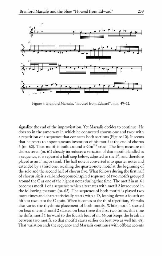
Branford Marsalis and the blues “Housed from Edward” 239
Figure 9: Branford Marsalis, “Housed from Edward”, mm. 49–52.
signalize the end of the improvisation. Yet Marsalis decides to continue. Hedoes so in the same way in which he connected chorus one and two: witha repetition of a sequence that connects both sections (Figure 10). It seemsthat he reacts to a spontaneous invention of his motif at the end of chorus5 (m. 60). That motif is built around a Gm7[5 triad. The first measure ofchorus seven (m. 61) already introduces a variation of that motif: Handled asa sequence, it is repeated a half step below, adjusted to the F7, and thereforeplayed as an F major triad. The half note is converted into quarter notes andextended by a third one, recalling the quarter-note motif at the beginning ofthe solo and the second half of chorus five. What follows during the first halfof chorus six is a call-and-response-inspired sequence of two motifs groupedaround the C as one of the highest notes during that time. The motif in m. 61becomes motif 1 of a sequence which alternates with motif 2 introduced inthe following measure (m. 62). The sequence of both motifs is played twomore times and characteristically starts with a D, leaping down a fourth orfifth to rise up to the C again. When it comes to the third repetition, Marsalisalso varies the rhythmic placement of both motifs. While motif 1 startedon beat one and motif 2 started on beat three the first two times, this timehe shifts motif 1 forward to the fourth beat of m. 66 but keeps the break inbetween two motifs, so that motif 2 starts earlier on beat two as well (m. 68).That variation ends the sequence and Marsalis continues with offbeat accents

240 Wolf-Georg Zaddach
Figure 10: Branford Marsalis, “Housed from Edward”, mm. 60–69.
and a strong laid-back phrasing (mm. 68ff.) which counteracts the regularflow of the previous motifs and sounds rather ragged.
During the last three measures of that chorus (mm. 70–73), Watts again startsplaying a triplet-influenced groove that continues until the beginning ofchorus eight. His triplets stabilize at the end of chorus six into a group of twotriplets which he repeats several times. With this continued superimpositionWatts creates a rhythmic displacement of the swing accents on two and fourand thereby, in combination with Hinton’s continued walking bass linein quarter notes, a certain tension and fragility. Marsalis picks up Watts’srhythmic intention immediately after his introduction in m. 72 (Figure 11).Instead of playing single quarter notes, he splits them up into two eighths,still interrupted and somehow ragged, while the tonal material is inside andoutlines the underlying chord progression. At the end of m. 73, he slowlycombines that rhythmic motif with Watts’s triplet motif, a varying two-notemotif, and lines in triplet feeling. He starts playing additional notes as wellas outside notes, such as the minor third over a B[7 (mm. 74, 78), the sharpeleventh over an F7 (m. 75), the flatted ninth over a D7 and C7 (mm. 80 and82), as well as the flatted fifth over the Gm7 again (m. 81). During the secondhalf of this chorus, he even doubles the triplet feeling and plays sixteenth-note triplets. At that point, he creates another high point by repeating anascending motif with the target tone C, starting from a C below and varyingthe tonal material in between just slightly by repeating the motion threetimes. As stated previously, Watts stops playing his superimposition rightat beat one of chorus eight, and Marsalis ends his intense phrase in chorusseven on the same accent.
During chorus eight and nine, Marsalis works with the previously mentionedtone repetition (mm. 90 and 91) and varies it into fast and repeated trills builtaround the same notes of C and D with a rhythmic placement on beat threefor each trill (mm. 106–108). Additionally, he once more emphasizes the

Branford Marsalis and the blues “Housed from Edward” 241
Figure 11: Branford Marsalis, “Housed from Edward”, mm. 72–76.
blues by oscillating between the minor and the major third over the F7 rightat the beginning of chorus nine (m. 97). In the last chorus, Marsalis refersagain to the theme with half notes on F placed on beat two, embellished, andapproached from faster notes from below (mm. 109 and 111). The referencesback to the theme and its variation in the first chorus are obvious and givethe solo some kind of closure. Yet, due to the continuation of the solo afterthe high point in chorus five, the end isn’t necessarily predictable.
The solo is followed by a bass solo, which mainly outlines the chord progres-sion in walking bass lines. Marsalis’s second solo spans over two choruses.Here, he emphasizes the bluesy minor third of F7 as a kind of anchor tone,frequently repeated and approached throughout the chord changes as thehighest pitch. He repeats the A[ and F in a trill in mm. 14 and 15, in somesense recalling blues and boogie piano trills. The band slows down a bit from127 bpm to 122 bpm and the share of syncopated tones played by Marsalis isslightly higher than during the first solo (35.6 % compared to 31.5 %). Thesong ends with a repetition as well as a variation of the theme, with the drumsstrolling out.
Conclusion
Marsalis’s first entire recording in a trio setup without a harmony instru-ment has a remarkable inclusion of traditional jazz sounds. Especially theblues “Housed from Edward” supports that impression. The traditional bassplaying by Hinton and the setup both enable Marsalis balance out traditionalimprovisation techniques with postbop devices. A focus lies on the creationand variation of simple melodies that effectively fit the blues. Here, Marsalisapplies call-and-response-inspired motivic work as a typical feature of tradi-tional blues. These ideas are contrasted with fast lines that utilize postbopdevices such as side-stepping and the superimposition of chord progressions.

242 Wolf-Georg Zaddach
Yet Marsalis embeds those modern sounds in larger melodic ideas such asimplied guide-tone lines that are built around the major and minor thirdof F7, again emphasizing the blues. The dramaturgy of the solo is the mostoutstanding overall characteristic. After reaching a peak in terms of eventdensity and usage of postbop devices in chorus five, he continues for anotherfive choruses, following a stream of motivic inventions and an interplay withWatts on the drums.
The solo as well as Marsalis’s approach to play the blues in a trio setupwith Milt Hinton on bass could be understood as a meditation or aestheticreflection on his own processes of accumulating and internalizing jazz historyand tradition—from the perspective of a postbop player who had alreadygathered diverse musical experiences at the time. The recording of “Housedfrom Edward” is an outstanding testimonial of a saxophonist who grew upin New Orleans and became involved in contemporary jazz in Boston andNew York City in the search to flourish and to establish his own voice ofmany facets.

Bob Berg’s solo on “Angles”
Klaus Frieler
Introduction
The present study attempts to reconstruct the creative processes underlyinga specific jazz solo improvisation—Bob Berg’s solo on “Angles”—using allavailable data from the musical surface as provided in the Weimar Jazz Data-base. To this end, we also try to integrate classical and computational analysismethods to gain a more complete picture than might be possible with eithermethod alone. This includes general statistical descriptions, a look at tonaland intervallic choices as well as the metrical and rhythmical design. Centralto our analysis will be an attempt to re-tell the ‘story’ of the solo with aspecial focus on playing ideas (midlevel units) and dramaturgic curves. Wealso take a closer look at the construction principles for lines, including aclassification of line types, and in conclusion investigate the usage of intervaland pitch patterns in order to arrive at a maximally complete picture of thecreative devices and processes involved.
The object under study is a solo by Bob Berg (1951–2002), who was aneminent postbop tenor sax player of Miles Davis fame. He was born inBrooklyn, New York, and of Italian-Jewish origin. Unfortunately, only verylittle information is available about his life and personality. What is known isthat he started playing saxophone at age 13 and studied at the Juilliard School,but never graduated. He became a professional musician already at the age of18 and immersed himself in the New York loft jazz scene. He also dippedbriefly into free jazz at the end of the 1960s. He was strongly influenced byJohn Coltrane and, in the 1970s, he initially shunned the then very popularfusion jazz, preferring more classical settings. From 1973 to 1976, he workedwith Horace Silver, and was part of Cedar Walton’s band from 1977 to 1981.His first record as a leader was New Birth from 1978, which featured CedarWalton on keyboards and piano. In the 1980s, Bob Berg came to the attention

244 Klaus Frieler
of Miles Davis, who included him in his famous electric band from 1984to 1987, where he became known as an eminent fusion saxophonist. Afterhe left Davis’s Band, Bob Berg diversified his interests and played postbop,fusion, and other styles in various settings and groups. In an interview from1996, he stated: “I feel pretty comfortable moving between different areas ofmusic.” Amongst others, he was a frequent collaborator with his band matefrom the Miles Davis band, guitarist Mike Stern, and with another Davisalumnus, Chick Corea, on whose Stretch label he also released several albums.After his untimely death in a tragic car accident in 2002, Berg left a musicallegacy of 12 records as a leader and 33 records as a sideman.
The piece “Angles” is a Bob Berg original from his 1993 record Enter theSpirit. The composition can be described as a typical postbop tune, witha chord progression that is halfway between tonality and modality, verymuch in the spirit of Wayne Shorter’s compositions from the 1960s. Thetheme melody is angular, which might have been an inspiration for the titleof the song. The form and chords of the theme are not maintained duringthe solos; instead, a simplified 48-bar scheme AAB of 16 bars each is used,with four chords lasting over four bars each (cf. Table 1). The tonality is notfully clear, but a tendency to A[ major can be stated, since the A sectionsstart with A[maj7 and end with E[7 and most of the chords more or less fitinto A[major. Deviations can be found in the D[7(]11) in the A and B sections,which belong to G[ major/minor, as well as in the altered G7]9 and D7alt
chords at the ends of the B sections, which do not fit into A[major and havea rather unusual falling fourth relationship. The D7alt leads back to the A[maj7
with a tritone step, and hence these two chords might be interpreted as asemitone downward shifted variant of a A[7–E[7 connection, which wouldfit better tonally. Due to the unusual chord connections, the overall loosetonality and rather long chord lengths, the solo form is located somewherebetween tonal and modal conceptions.
The tempo is rather high with 270 bpm and the rhythmic feel oscillatesconstantly between latin in the A sections and swing in the B sections. Theaccompaniment is very dense. In particular, pianist David Kikoski playing isrhythmically very accentuated, relentlessly pushing the energy, while oftenfilling the phrase gaps in Berg’s solo with rhythmical impulses. DrummerDennis Chambers employs a modern, complex and busy drum style, whilefrequently reacting to Berg as well as driving him forward.
The solo comprises 799 tones in 38 phrases and 144 bars over three choruses.Most of the tones (85.4 %) are very short on an absolute scale (i. e., absoluteduration class) which in this high tempo equals mostly the level of eighthnotes (cf. Table 2). The syncopicity, i. e., the percentage of syncopated tones,

Bob Berg’s solo on “Angles” 245
Table 1: General characteristics of Bob Berg’s solo on “Angles”.
Composer Bob BergRecord Enter the Spirit (1993)Personnel Bob Berg (ts), David Kiskoski (p),
James Genus (b), Dennis Chambers (dr)Tempo 270 bpmSignature 4
4
Key Mostly A[ majorForm A(16) A’(16) B(16)
4-bar chord changes throughoutChord Changes A: A[maj7 | Cm7 | D[7 | E[7 |
B: Fm7 | D[7]11 | G7]9 | D7alt |Rhythm feels (theme) A: Latin, B: SwingRhythm feels (solos) A: Latin, B: LatinLengths 799 tones
144 bars3 choruses8 phrases
Duration 127 sDensities 6.3 tones/sec
5.6 tones/bar21 tones/phrase
Metrical centroid 3+Start of phrases 42 % (beat 3)
13 % on 3+10 % on 110 % on 2+
Syncopicity 9.2 %Tessitura A[3−A[5
(36 semitones / 3 octaves)
is rather low (9.4 %) compared to the average value of about 30 % in theWeimar Jazz Database. This seems to be mostly due to Berg’s highly precisetiming, since, due to the metrical annotation with the FlexQ algorithm (cf.Chapter Computational melody analysis), syncopicity values in the WeimarJazz Database are partly driven by laid-back playing and rhythmical freedom.The listening experience corroborates this conjecture, as Berg’s solo shows avery tight rhythmical performance.

246 Klaus Frieler
A1 A1 A1 A1 A2 A2 A2 A2 B1 B1 B1 B1
A1 A1 A1 A1 A2 A2 A2 A2 B1 B1 B1 B1
A1 A1 A1 A1 A2 A2 A2 A2 B1 B1 B1 B1
3
2
1
97 101 105 109 113 117 121 125 129 133 137 141 145
49 53 57 61 65 69 73 77 81 85 89 93 97
1 5 9 13 17 21 25 29 33 37 41 45 49
4050607080
4050607080
4050607080
Bar number
MID
I Pitc
h
Figure 1: Piano roll representation of Bob Berg’s solo. The single panels correspondto choruses. Phrases are colored alternatively; form parts are shaded with differentgray tones.
The metrical placing of tones is uniformly distributed over all eighth notepositions in the 4
4 bar (Figure 2, middle panel). Interestingly, Berg has a strongpreference for starting his phrases on and around the third beat of a bar(Figure 2, top panel; Table 1). As can be seen in Table 3, 22 of all 38 phrasesstart on beat 3, very often (ten times) also right after a chord change (seealso Figure 1 for a visual overview of the interplay of phrase lengths, formsections, and four bar units). Another interesting fact is that Berg nearlyalways continues his phrases over the changes of contrasting form sections,i. e., A2→B1 and B1→A1, but not on the transition A1→A2. The change ofrhythm between the A and B sections under an ongoing phrase has a certainsurprise effect and also contributes to the flow of the solo. The phrase endingsare more diversely distributed but tend to fall on on-beats and also on themetrically strong first and third beats of a bar (Figure 2, lower panel).
With respect to accentuation in loudness, Berg shows a certain tendency toplay (mostly in his fast lines) four eighth groups with descending loudness,starting from the strong first and third beat (Figure 3).

Bob Berg’s solo on “Angles” 247
Table 2: Distribution of absolute and relative duration classes.
Duration Class Absolute (%) Relative (%)
very short 85.4 9.9short 12.0 78.3medium 1.9 9.4long 0.6 1.6very long 0.1 0.8
Table 3: Distribution of metrical and hypermetrical positions of phrase beginnings.
Bar phase Beat position Sum1 2 3 4
0 1 1 10 0 121 4 2 4 1 112 1 2 6 1 103 2 1 2 0 5
Sum 8 6 22 2 38
Note. Bar phase= distance in bars from a chord change / four-bar block. Beat position= beat in the bar disregarding tatumposition.
Tonal and interval choices
The overall pitch range is three octaves from A[2 to A[5, with a strong focuson the middle octave; 83 % of all tones are between A[3 and E[5 (Figure 4, top).Tonally, the pitch classes fit very well into A[ major, even though G is themost common pitch class (accordingly, G4 is the most common tone), but thisis due to some repeating patterns (‘oscillations’) in the third chorus, where G4is the central tone. Looking at the pitch class distribution (Figure 4, bottom)the A[ major seems to be rather dominant, with about 84 % of all tonescoming from A[ major. However, the solo makes a much more chromaticimpression during listening. This can be explained by looking at the chordaldiatonic pitch class distribution (Figure 5) and the chord-wise distribution ofnon-diatonic tones (Figure 6). There is a clear contrast between very inside,sometimes pentatonic playing on the one hand, and highly chromatic andeven outside playing on the other hand. The latter mostly takes place in thesecond half of the B sections over the altered dominant seventh chords G7]9
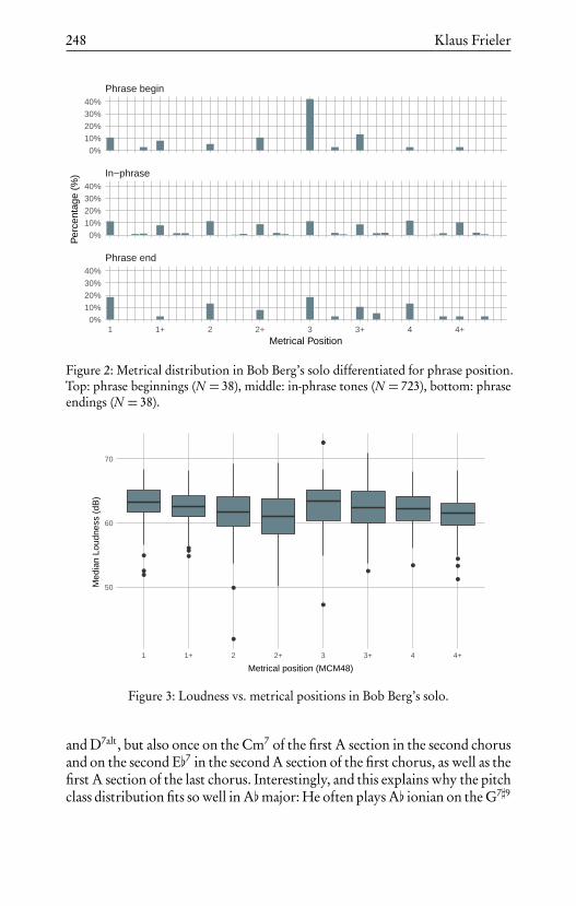
248 Klaus Frieler
Phrase end
In−phrase
Phrase begin
1 1+ 2 2+ 3 3+ 4 4+
0%
10%
20%
30%
40%
0%
10%
20%
30%
40%
0%
10%
20%
30%
40%
Metrical Position
Per
cent
age
(%)
Figure 2: Metrical distribution in Bob Berg’s solo differentiated for phrase position.Top: phrase beginnings (N = 38), middle: in-phrase tones (N = 723), bottom: phraseendings (N = 38).
50
60
70
1 1+ 2 2+ 3 3+ 4 4+
Metrical position (MCM48)
Med
ian
Loud
ness
(dB
)
Figure 3: Loudness vs. metrical positions in Bob Berg’s solo.
and D7alt, but also once on the Cm7 of the first A section in the second chorusand on the second E[7 in the second A section of the first chorus, as well as thefirst A section of the last chorus. Interestingly, and this explains why the pitchclass distribution fits so well in A[major: He often plays A[ ionian on the G7]9
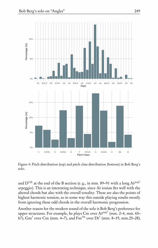
Bob Berg’s solo on “Angles” 249
0%
5%
10%
A2 B2C3 D3 E3F3 G3 A3 B3C4 D4 E4F4 G4 A4 B4C5 D5 E5F5 G5 A5Pitch
Per
cent
age
(%)
0%
5%
10%
15%
C C#/Db D D#/Eb E F F#/Gb G G#/Ab A Bb BPitch Class
Per
cent
age
(%)
Figure 4: Pitch distribution (top) and pitch class distribution (bottom) in Bob Berg’ssolo.
and D7alt at the end of the B section (e. g., in mm. 89–91 with a long A[maj7
arpeggio). This is an interesting technique, since A[ ionian fits well with thealtered chords but also with the overall tonality. These are also the points ofhighest harmonic tension, so in some way this outside playing results mostlyfrom ignoring these odd chords in the overall harmonic progression.
Another reason for the modern sound of the solo is Bob Berg’s preference forupper structures. For example, he plays Cm over A[maj7 (mm. 2–4, mm. 65–67), Gm7 over Cm (mm. 4–7), and Fm7[5 over D[7 (mm. 8–19, mm.25–28).

250 Klaus Frieler
Table 4: Mean and median of chordal diatonic pitch classes mapped to third layers.See text for details.
Form section Chord Median Mean
A1 A[maj7 7.0 6.6Cm7 5.0 6.9D[7 5.0 6.7E[7 7.0 6.2
A2 A[maj7 7.0 7.1Cm7 7.0 6.3D[7 7.0 6.9E[7 7.0 6.3
B1 Fm7 5.0 6.3D[7]11 9.0 8.5G7]9 9.0 7.8D7alt 9.0 8.9
All 7.0 7.02
This observation can be corroborated by mapping chordal diatonic pitchclasses to third layers. This is done by mapping 1 and 3 to itself, and themappings (7, ]7, [7)→ 7, (2, [9, ]9)→ 9, (4, ]11)→ 11, and (6, [13)→ 13.Afterwards, mean and median values of the mapped chordal pitch class distri-bution are a measure for the amount of upper structures used. The resultscan be seen in Table 4, broken down by chords. The overall median is 7, i. e.,the seventh, which is right in the center of a chord’s expansion into thirds.The interval distribution is somewhat unusual, as can be seen in Figure 7.Compared to the overall interval distribution (lower panel), there are manymore tone repetitions but also a flat plateau for small descending intervals.This however can be explained by the long oscillating figures in mm. 75–81and mm. 95–108, in which similar figures are repeated very often. Theseoscillations are responsible for the unusual interval distribution, but arenevertheless very important for the solo as a whole.
Re-telling the story
The storytelling metaphor is an important aspect in jazz parlance and jazzresearch (Frieler et al., 2016b) and might also be an active guiding principlefor improvising jazz solos. Of course, there are no ‘real’ stories to be told

Bob Berg’s solo on “Angles” 251
Abj7
C−
7D
b7E
b7F
−7
Db7#11
G7#9
D7alt
1 2 3 4 5 6 7 #9 #7 #11 b7 #10 b9 b13
010203040
010203040
010203040
010203040
010203040
010203040
010203040
010203040
Extended Chordal Diatonic Pitch Class
coun
t
Figure 5: Tonal choices in Bob Berg’s solo broken down for individual four-bar chords.Dark blue: diatonic pitch classes; light blue: non-diatonic pitch classes.
Chorus 1
Chorus 2
Chorus 3
Abj7 C−7 Db7 Eb7 Abj7 C−7 Db7 Eb7 F−7 Db7#11 G7#9 D7alt
0%
20%
40%
60%
0%
20%
40%
60%
0%
20%
40%
60%
Chords
Non
−di
aton
ic T
ones
(%
)
Figure 6: Outside playing in Bob Berg’s solo for each chorus. Chords are listed as theyappear in the AAB form.

252 Klaus Frieler
All Tenor Solos
Angles
−12 −11 −10 −9 −8 −7 −6 −5 −4 −3 −2 −1 0 1 2 3 4 5 6 7 8 9 10 11 12
0%
5%
10%
15%
0%
5%
10%
15%
Semitone Interval
Per
cent
age
(%)
Figure 7: Semitone interval distribution in Bob Berg’s solo (top) and in all other tenorsax solos in the Weimar Jazz Database (bottom).
in music due to the lack of denotative meanings. Nevertheless, a certaindramaturgy might be discernible, which might or might not follow narrativeprototypes (e. g., the narrative arc).
In the following sections, we will first try a re-narration of the entire solo,based on midlevel units, and then have a look at global dramaturgic shapes.
Midlevel Analysis
Midlevel analysis is a qualitative annotation system for jazz solos which areinspired by playing ideas and called ‘midlevel units’ (MLU, cf. p. 54 andFrieler et al., 2016a). There are nine main types of midlevel units (MLU) (line,lick, melody, rhythm, expressive, theme, quote, void, fragment) with 16 sub-and 38 sub-subcategories.
In Figure 8, a piano roll representation of the solo broken down into the maintypes of MLUs is depicted. The solo transcription in Figure 17 can be foundannotated with full MLU types. Finally, in Table 6 a complete run-down ofthe sequence of MLUs in this solo is listed.
In this solo, 51 MLUs of only five main types are used: line (21), lick (11),melody (6), rhythm (6), expressive (6). 13 MLUs are glued together to form
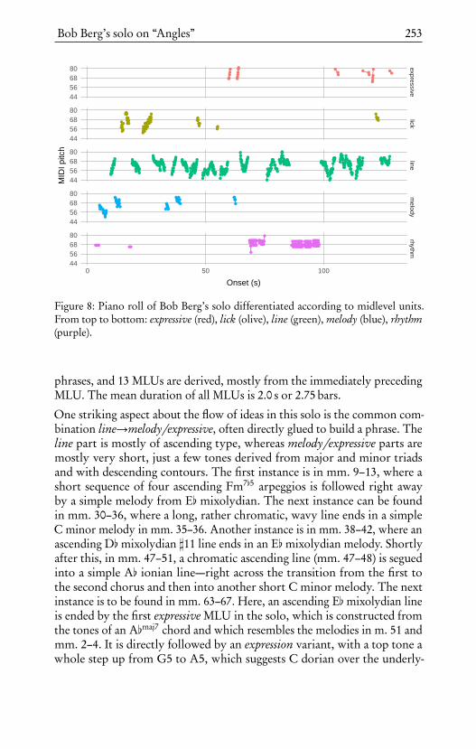
Bob Berg’s solo on “Angles” 253
expressivelick
linem
elodyrhythm
0 50 100
44566880
44566880
44566880
44566880
44566880
Onset (s)
MID
I pitc
h
Figure 8: Piano roll of Bob Berg’s solo differentiated according to midlevel units.From top to bottom: expressive (red), lick (olive), line (green), melody (blue), rhythm(purple).
phrases, and 13 MLUs are derived, mostly from the immediately precedingMLU. The mean duration of all MLUs is 2.0 s or 2.75 bars.
One striking aspect about the flow of ideas in this solo is the common com-bination line→melody/expressive, often directly glued to build a phrase. Theline part is mostly of ascending type, whereas melody/expressive parts aremostly very short, just a few tones derived from major and minor triadsand with descending contours. The first instance is in mm. 9–13, where ashort sequence of four ascending Fm7[5 arpeggios is followed right awayby a simple melody from E[ mixolydian. The next instance can be foundin mm. 30–36, where a long, rather chromatic, wavy line ends in a simpleC minor melody in mm. 35–36. Another instance is in mm. 38–42, where anascending D[mixolydian ]11 line ends in an E[mixolydian melody. Shortlyafter this, in mm. 47–51, a chromatic ascending line (mm. 47–48) is seguedinto a simple A[ ionian line—right across the transition from the first tothe second chorus and then into another short C minor melody. The nextinstance is to be found in mm. 63–67. Here, an ascending E[mixolydian lineis ended by the first expressive MLU in the solo, which is constructed fromthe tones of an A[maj7 chord and which resembles the melodies in m. 51 andmm. 2–4. It is directly followed by an expression variant, with a top tone awhole step up from G5 to A5, which suggests C dorian over the underly-

254 Klaus Frieler
ing Cm7. After this instance, which is a first peak moment in the solo, theseries of longer oscillations starts. The next instance of the model is then tobe found at the beginning of the third chorus (mm. 113–117), introducedhere by a long-reaching, arpeggiated ascending line, ending in a C minortriad-based melody. An intensified variant can then be found a few bars later,in mm. 126–132, where the melody at the end is modified a bit to accommo-date the Fm7 chord. Again a few bars later, in mm. 134–136, a shortened andupwardly transposed echo follows, itself immediately succeeded by a lick,which resembles the melody in mm. 41–42. Finally, the very last phrase, inmm. 138–144, starts out with a faint echo of the oscillations from the secondchorus, and then mutates into a short chromatic passage, segueing into adiatonic ascending arpeggio which ends in a short, two-tone expressive MLU.In a way, these very last seven bars contain the whole solo and its main ideasin a nutshell, functioning somewhat as a short conclusion.
The technique of ending a line with a short melodic part, often with longertone durations, could be dubbed ‘piggy tailing’. In many solos, the ‘piggytails’ consist of only a few tones, normally one to three, which function as ashort deceleration bringing a fast line to halt. One example for a more typical‘piggy tail’ can be found in m. 124.
It interesting to look at ideas that occur only once in the solo. First, thereis a Parker-sounding lick in m. 14–15 which is glued to a piggy tail melody.Indeed, the interval sequence (−3,−4,−5,+3,−2,+1), starting on the thirdbeat in m. 14, can be found three times in the Charlie Parker Omnibook.
Then, there is a very short rhythm_single_irregular in m. 18–19, which func-tions as an interruption of a longer line, even though the MLU right beforeit is labeled lick. Without this short intermission the whole complex wouldbe just one long wavy line.
Generally, there is a shortage of short licks in this solo. Measures 24–28 presentan ascending sequence of licks, which consists of Fm7[5 arpeggios, nearly thesame as the ones in mm. 9–11, but here extended higher and played in aspecific ‘choppy’ rhythm, which transforms it into a sequence of licks. This isa good example of how the same sequence of pitches can be transformed intosomething distinctively different by only changing the rhythm—in this caseby prolonging some inter-onset intervals. After he reaches the same endpoint(E[5) as in m. 11, Berg continues with a very short and abridged version ofm. 12, which sounds as a descending answer to the ascending arpeggios.
In m. 49, in the first bar of the second chorus, when the rhythm group shiftsback from swing to latin, Berg plays his only embellishment figure in theentire solo, which vaguely recalls a pop jazz saxophone lick, but which isfully integrated in a much longer line of mixed character (cf. p. 256).

Bob Berg’s solo on “Angles” 255
At the end of the first A section in the second chorus, in m. 60–62, thereseems to be a short black-out in the flow of the solo. First, after finishing thelong seven-bar line that started in m. 53, Berg continues with a very short lick,which is basically a transposed version of the ‘piggy tail’ of the line (m. 59).This sounds either as a bold confirmation of the preceding line, a false start ofanother line, or as a moment to gain time. After a bar-long pause, he embarksin mm. 61 and 62 on a short line, which is basically an E[9 arpeggio over theE[7 which does not sounds fully convincing, neither tonally nor in regardto phrasing. Next, as if ‘upset’ about this rather weak passage, he expressesthat anger with a short diatonic up-swing (mm. 63 and 64) right into the firstexpressive MLU in the solo, which brings G5, the highest pitch so far, heldfor over one bar.
The last one-time element in this solo can be found in mm. 86–89, where Bergplays a mixed E[/E[+ descending arpeggio with a constant eighth/dottedquarter rhythm pattern with tone repetitions (line_i_dd) over the D[7]11.From that point on, all the remaining material is in one way or anotherrelated to some preceding material.
Dramaturgy
The dramaturgy of Berg’s solo seems to be well-crafted, either intentionallyor as emerging from group interaction. The general tension curve is doublyarched. This can be seen on one hand in the event densities across the courseof the solo. In Figure 9, the number of tones of two-bar units shifted bar-wisealong the time axis and plotted against the onset of the first tone of the barunit is depicted, along with a polynomial trend. From the beginning on, theevent density increases constantly over a long stretch and then dips downat the beginning of the second chorus to increase even more towards theend of the second chorus, where the highest densities are reached with thesequences of oscillations. The third chorus then sees a slow decay, but thisdoes not mean that the intensity decreases, it is merely shifted to anotherdimension. This can be seen in Figure 10 where pitch and loudness curves of20 note windows (with a hop-size of 10 tones) are plotted against the onsetsof the windows. Both curves show an overall ascending trend—particularlythe loudness curve—with some oscillations. One sees that the pitch heightsrise quite rapidly in the first chorus but drop towards the beginning of thesecond chorus, to rise continually towards the end. In the third chorus, acertain saturation is reached, but in fact with strong oscillations, showing astark contrast (at about 100 s). All in all, a clear peak in global intensity isreached with the sequence of oscillations.

256 Klaus Frieler
5
10
15
20
25
0 50 100
Onset (s)
Num
ber
of to
nes
Figure 9: Event densities (number of tones) of Bob Berg’s solo for windows of twobars shifted bar-wise along the solo.
This overall dramaturgy is also reflected in Figure 8. The melody and lickMLUs appear mostly in the first chorus whereas the second chorus is dom-inated by the sequence of oscillations. The expressive MLUs appear for thefirst time at the beginning of the second chorus, and take over the role of themelody afterwards. This has an effect of intensification. The third chorus isthen built from the double sequence of line–expressive and line–line–expressive–expressive, and resolves, finally, in the epitomic phrase line–expressive at thevery end.
Line construction
The analysis of the MLU content of the solo shows that Berg utilizes dif-ferent kind of lines in his solo: diatonic lines, arpeggios, chromatic lines,and mixtures thereof. To gain further insights, we manually classified the 21line MLUs using this four-fold classification scheme and found four diatonic,three chromatic, six arpeggiated, and eight mixed lines. They indeed differwith respect to their interval content, as the distributions of frequencies ofsemitones, whole tones, and thirds show (Figure 11).
Using a similar system, we also classified line segments of seven intervals bymoving this window by four elements. Segments always start at the beginning

Bob Berg’s solo on “Angles” 257
Pitch
Loudness
0 50 100
55
60
65
70
58
60
62
64
66
Onset (s)
Val
ue (
dB)/
MID
I Pitc
h
Figure 10: Smoothed pitch and loudness curves for Bob Berg’s solo. Smoothing wasdone with windows of 20 tone events and a hop size of 10 tones. Trend line fittedwith a polynomial of 6th degree.
Arpeggiated Mixed
Chromatic Diatonic
Semitones Whole Tones Thirds Jumps Semitones Whole Tones Thirds Jumps
0%
20%
40%
60%
0%
20%
40%
60%
%
Figure 11: Interval content of the four line types found in Bob Berg’s solo.
of line MLUs. A segment is classified as ‘pentatonic’ if thirds and whole tonesaccount for more than two thirds of the intervals (i. e., five or more). It is

258 Klaus Frieler
classified as ‘arpeggio’ if thirds and larger intervals account for more than twothirds of the intervals. It is classified as ‘diatonic’ or ’chromatic’, if semitonesand whole tones account for more than two thirds of the intervals, and thendepending on whether there are more semitones (‘chromatic’) or whole tones(‘diatonic’). Finally, segments are classified as ‘mixed’ if they do not fulfillany of these criteria or if the difference between the first and second mostfrequent class is less than 0.1. In Figure 12, the sequences of segment classesare plotted for each line in the solo. The first observation is a slight preferencefor mainly pentatonic lines (e. g., lines 1, 2, 4, 9, 18), although there is anequal share of pentatonic and mixed line segments (30.0 % each). The nextcommon segment type is ‘chromatic’ (20.8 %), followed by arpeggios (13.3 %),and ‘diatonic’ 5.8 %. The length of lines ranges from 3 (line 8, 9, 11, 13) to 12segments (line 7), with a median of 5.5. For the series of segment types, noobvious patterns can be identified, except that a segment type has a strongtendency to be repeated (about 50 %), which is partly due to the constructionof our measure. Furthermore, chromatic segments tend to occur earlier ina line (mean normalized position = .45), whereas diatonic and pentatonicsegments tend to occur later (mean normalized positions of .68 and .64). Withrespect to the entire solo, however, pentatonic segments tend to occur earlier,and arpeggios tend to appear later (e. g., in the third chorus, mm. 113ff. andmm. 126ff.). All in all, Berg shows a great variability in his approach to lineconstruction.
Pattern usage
To investigate the usage of patterns in Berg’s solo, we used the partitionfunction of the melpat module in the MeloSpyGUI with all seven Berg solosin the Weimar Jazz Database as a background corpus. Since the rhythmsare rather uniformly based on eighth notes due to the abundance of lines,we only calculated interval and pitch patterns and no rhythmical patterns.For the interval domain, we extracted patterns with at least N ≥ 5 intervals,which correspond to at least six tones. For the pitch domain, we demandedN ≥ 6. For both cases, we extracted patterns that occur at least twice, butplaced no restriction on the number of solos they should appear in.
We found 147 interval patterns meeting these conditions, with a coverage of64.8 %, i. e., about two thirds of the tones in Berg’s solo are contained in aninterval pattern of at least five intervals that occur at least twice somewherein the seven Berg solos under consideration. This is the highest coverage ofall Berg solos, which have a mean coverage of 56 %. But this is partly due tothe extensive oscillations in the solo. However, when using all postbop tenor

Bob Berg’s solo on “Angles” 259
Line 17 Line 18 Line 19 Line 20
Line 13 Line 14 Line 15 Line 16
Line 9 Line 10 Line 11 Line 12
Line 5 Line 6 Line 7 Line 8
Line 1 Line 2 Line 3 Line 4
chr
dia
pen
arp
mix
chr
dia
pen
arp
mix
chr
dia
pen
arp
mix
chr
dia
pen
arp
mix
chr
dia
pen
arp
mix
Line
Typ
e
Figure 12: Classification of segments of seven intervals for line MLUs in Bob Berg’ssolo. Hop size is four intervals, i. e., points are separated by four notes each. chr= chro-matic, dia = diatonic, pen = pentatonic, arp = arpeggio, mix =mixed.
solos, the coverage rises to 80.7 %, which is close to the mean coverage of78.3 %.
We found 81 pitch patterns, with a coverage of 46.8 % (mean coverage acrossall Berg solos: 40.6 %). See Figure 13 for a display of interval and pitch patternsin Berg’s solo. The longest patterns are produced by the oscillations and arenot shown.
As expected, there are fewer pitch patterns than interval patterns (because apitch pattern is automatically also an interval pattern, but not vice versa). Theshorter patterns are more volatile, whereas the very long interval patterns arealso pitch patterns, which shows that they are specifically rehearsed and then

260 Klaus Frieler
Interval Pattern
Pitch Pattern
68
1012141618
68
1012141618
0 200 400 600 800
Tone position
Pat
tern
leng
th
Figure 13: Interval (top) and pitch patterns (bottom) in Bob Berg’s solo on “Angles”with an effective length of at least six occurring at least twice in the seven solos byBerg in the Weimar Jazz Database. Only patterns up to an effective length of N = 18are shown, since the longest patterns are due to the oscillations.
reproduced. The shorter patterns are probably rehearsed in many differentkeys and thus can be used as building blocks, e. g., for line constructionin many different harmonic situations. To illustrate the pattern usage byBob Berg in this particular solo a little further, we produced a network ofpattern similarities for the interval patterns. To this end, we calculated editdistances between patterns. The edit or Levenshtein distance (Levenshtein,1965; Müllensiefen & Frieler, 2004) is defined as the minimum number ofeditions, deletions, and substitutions required to transform one sequenceof symbols (here: intervals) into the other. For two completely differentsequences of different length, the maximum number of operations is thelength of the longer sequence. This can be used to convert the edit distanceinto similarity values between 0 and 1. The full matrix of similarities betweenall interval patterns was then converted into an adjacency matrix using athreshold of 0.5. This means that all similarities lower than .5 were set to 0and all similarities above .5 were set to 1. These values were used to create asimilarity network by feeding them into a graph representation algorithmfrom the network package for R (R Development Core Team, 2008). Theresult can be seen in Figure 14.

Bob Berg’s solo on “Angles” 261
x73
k72y69
a30
i62
x75
a68
x56
h72
c50
p67
s44
f28
y29
v73
t76
n40
w75
z64
p48
b12
e31
l18
h44
v54
h41
u64j64
q66
e70b74y62
p68
m18
j66
b70
g73
k73
a64
k66
b65
d74
v26
m38
a44
v44r28
y27
s43
w64
m39
t69o55
j54
p69
z56w
63
u68
z28
t59
w55
w71
b66
g74
u69
x58
v53
v64
p61
a73
v71 c53a55
e59
l70
c46
j72
m28
d45s42
Figure 14: Network representation of all interval patterns in Bob Berg’s solo. Edgesare drawn according to pattern similarities, which were calculated using edit distanceand range from 0 to 1, where a value of 1 means identity. Only connections withsimilarity greater than 0.5 shown. Node labels are arbitrary tags assigned by thepartition algorithm.

262 Klaus Frieler
−1,−1,−1,−1,2,2,3
−2,1,1,−2,1,−1,−1,−1,−1,2,2,−4,2,−1,−1,4,−2
1,−1,−1,−1,−1,2,11,−2,1,−1,−1,−1,−1,2,2
−1,−1,−1,−1,2,2,−4,2,−1,−1,4,−2,−3
−1,−1,−1,−1,2,2,−4,2,−1,−1,4,−2,−4
−1,1,1,−2,1,−1,−1,−1,−1,2
−1,−1,−1,−1,2,2,3,−1
−1,−1,−1,2,1,2,−3
−4,−1,−1,−1,2,1,2
−1,−1,−1,−1,−3
−1,−1,2,−1,−1,−1,−1,−1,2,2−1,−1,−1,−1,4
Figure 15: Close-up of the upper middle cluster of the full pattern network. Nodelabels are pattern values; edge widths are proportional to similarity.
One sees two clusters of strongly interconnected patterns and one rather loosecluster. There are also a few small cluster of only two or three highly similarpatterns as well as several singletons. To highlight the cluster structures inmore detail, we will have a closer look at the dense cluster in the upper middleof the network plot. It can be seen in Figure 15. A list of the patterns in thiscluster can be found in Table 5 and are shown in Figure 16. The pattern b12is the longest of all with 17 intervals (18 tones). It occurs twice in “Angles”(mm. 30 and 108) at the same metrical position and with identical pitches. Itconsists of a rather unpredictable sequence of mostly semi- and whole tones.Clearly, this pattern was pre-rehearsed. This is corroborated by the fact thatthe next two longest patterns, l18 and m18, are, except for their last tones,contained in pattern b12 as a suffix. On the other hand, pattern m28, apartfrom some slight rhythmical variation, is contained at the beginning of b12,as a prefix. However, it is counted as a separate pattern because it also occursin another solo by Bob Berg (on “You and the Night and the Music” from the1997 album Another Standard). The same holds true for pattern e31, which isfully contained in b12, but occurs five times in total in three different solos(there only as proper sub-patterns). All other patterns in this cluster are moreor less variations of the material from the above mentioned patterns.
The main core of this pattern cluster is the interval pattern -1, -1, -1, -1, 2, 2 offour descending semitones and two ascending whole tones, mostly realized

Bob Berg’s solo on “Angles” 263
Table 5: Upper middle interval pattern sub-network.
Tag MM. N FC FA Value
b12 30, 108 17 2 2 -2, 1, 1, -2, 1, -1, -1, -1, -1, 2, 2, -4, 2, -1, -1, 4, -2
l18 31 13 2 1 -1, -1, -1, -1, 2, 2, -4, 2, -1, -1, 4, -2, -3m18 43, 110 13 2 2 -1, -1, -1, -1, 2, 2, -4, 2, -1, -1, 4, -2, -4m28 140 10 2 1 -1, 1, 1, -2, 1, -1, -1, -1, -1, 2v26 54 10 4 1 -1, -1, 2, -1, -1, -1, -1, -1, 2, 2e31 30, 92, 109 9 5 3 1, -2, 1, -1, -1, -1, -1, 2, 2m38 55 8 2 1 -1, -1, -1, -1, 2, 2, 3, -1a44 55, 92 7 3 2 -1, -1, -1, -1, 2, 2, 3d45 140 7 2 1 1, -1, -1, -1, -1, 2, 1s42 141 7 6 1 -1, -1, -1, 2, 1, 2, -3s43 58 7 4 1 -4, -1, -1, -1, 2, 1, 2u64 34 5 3 1 -1, -1, -1, -1, -3v64 93 5 3 1 -1, -1, -1, -1, 4
Note. Tag= pattern name generated by the partition algorithm; MM.= measuresin “Angles” where pattern can be found; FC = frequency of pattern in the entireBob Berg sub-corpus in the Weimar Jazz Database; FA = frequency of pattern inthe solo on “Angles”.
in the middle octave starting from G4 and on a strong metrical position(first or third beat, only exception: v64). Only pattern u64 contains a slightlyshorter version (last interval is a descending minor third −3). Notably, thiscore pattern does not occur as an independent pattern in the pattern parti-tion, because it is always embedded in longer patterns. The most commoncontinuation is a whole tone up (all patterns except s32 and v64), followedeither by a descending major third or an ascending minor third.
Taken together, this pattern cluster alone shows clearly that Berg has a pre-rehearsed pattern vocabulary at his disposal, which is stable over time. It ismostly fixed in metrical and pitch position but can be varied by chainingdifferent sub-patterns to longer patterns with contextual adjustments.
Creative Devices
In the foregoing sections, we provided a rich description of Berg’s solo on“Angles” using many different perspectives. We would like to summarize herethe most important creative devices that are employed by Berg.
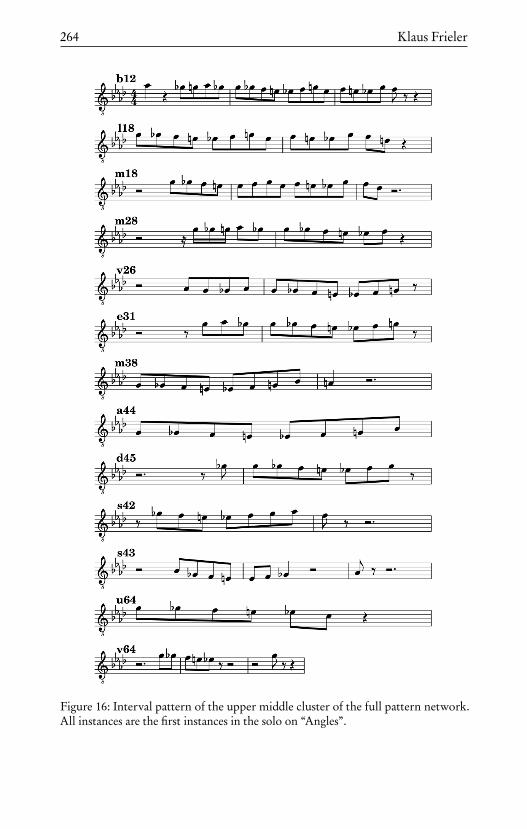
264 Klaus Frieler
Figure 16: Interval pattern of the upper middle cluster of the full pattern network.All instances are the first instances in the solo on “Angles”.

Bob Berg’s solo on “Angles” 265
First of all, the entire solo seems to follow a rather well-crafted dramaturgy.It shows a double arch shape with overall increasing energy. The dramaturgyseems to develop rather spontaneously and is partially driven by interactionswith the band. One characteristic of this solo is the frequent changes ofrhythm feel from latin to swing and back, which produce a tension andrelease pattern on the highest level. Berg nearly always continues his phrasesseamlessly over these changes in rhythmic feel, which adds to the flow of hisimprovisation and the impression of mastery and virtuosity.
On the level of playing ideas, the solo is characterized by an abundance oflines with a conspicuous absence of licks. Rather, the frequently long linesof variable types are contrasted with either pentatonic or diatonic melodieswhich become more expressive during course of the solo. These melodic licksoften occur at the end of a long line, and were dubbed ‘piggy tails’. Such smallextensions at the end of a longer line, or sometimes also at the beginning,can be frequently observed in jazz solos since bebop, but in this solo, theseare rather long and melodious (or expressive). Their general function mightbe to give a certain form of closure to a line and/or coming to a stop after afast-moving line. Sometimes, the effect is that the line feels like a mere upturnto its more melodious or expressive piggy tail.
As shown above, Berg constructs his lines very diversely, mixing penta-tonic/diatonic sections with (wide) arpeggios and chromaticism. These linesappear to be composed from preconceived patterns that Berg has in his vo-cabulary. Some of these patterns can be found in solos on the same recordbut also in solos played years later.
The contrast between pentatonic/diatonic material and chromatic and out-side material can be seen as a general feature of this solo. Though it is strictlyrooted in A[major, the frequent chromaticism as well as the ‘trick’ of playingthe main key over the outside harmonies D7alt and G7]9 at the end of eachchorus, i. e., essentially ignoring these chords, create tonal tension and relax-ation patterns which propel the solo forward. These parts are contrasted withmelodies of ostensible simplicity as well as with expressive outbursts. Theconstruction of lines with inside/outside elements as well as the inside vs. out-side contrasts of larger parts can be seen as a kind of self-similarity and mightresult from deliberate artistic decisions. Berg works by contrasting the simple(e. g., pentatonic, melody) with the complex (e. g., chromaticism, elaborateasymmetric lines) on different levels. This might also be reflected in anotherimportant element not only of this solo but also of many other postbop play-ers (e. g., Michael Brecker, Kenny Garrett, Chris Potter), namely the extensiveoscillating figures. These normally have an intensifying effect, especially ifplayed in ascending tonal sequences as in this solo. Compared to intricate

266 Klaus Frieler
bebop lines, these oscillations are simple in construction and rather easyto perform, hence early bebop pioneers such as Parker and Gillespie mighthave shunned them as they were used by Rhythm & Blues ‘honkers’. But theneed for heightened expressivity in the postbop style, probably starting withColtrane, (re-)introduced them into modern jazz improvisation, where theyserve as energetic counterparts to more sophisticated line constructions.
Finally, Berg frequently uses motivic relationships and tonal sequences tocreate musical logic and coherence. The use of long and very long patterns(e. g., pattern b12 and m18) and parts thereof might also contribute to a senseof coherence. Apart from a few single ideas, much of the material in this solois related in one way or another, sometimes subtly transformed and varied,sometime re-contextualized, sometimes re-used verbatim. In this regard, thevery last phrase (mm. 139–144) is remarkable as it subsumes the entire soloin a nutshell and is hence also an epitome for Berg’s coherent solo design.
Conclusion and outlook
This in-depth case study of a single solo attempts to retrace the underlyingcreative processes. As a case study, its power for generalizations is of courselimited, but a large collection of similar in-depth case studies along with large-scale contextualization in a corpus might finally converge to form a stable andgeneral model of jazz improvisation. We can state for now, however, that theresults presented here are compatible with a three-level hierarchical model.The highest level is the overall dramaturgy of the solo, created in interactionwith the band, which results in the decisions for certain playing ideas onthe middle level, e. g., lines, melodies, expressive moments, oscillations etc.,which are then—on the lowest level—realized by combining preconceivedmaterial on one hand and spontaneous out-of-the-moment inventions onthe other. However, the last point has to actually been proven yet. The sub-corpus of Berg’s solos in the Weimar Jazz Database is rather small. For thefuture, it would be highly desirable to gather a much larger collection to seewhether certain elements, such as the melodic ‘piggy tails’ and the oscillationpatterns, were indeed invented on-the-fly or whether pre- or postdecessorscan be found in Berg’s oeuvre.
Finally, the selection and pre-creation of the material, e. g., their tonal con-struction, seem to be highly specific for Berg’s personal style but are nonethe-less shaped by a general stylistic sensitivity.

Bob Berg’s solo on “Angles” 267
Table 6: Run-down of MLUs in Bob Berg’s solo on “Angles”.
Measures MLU Scale Comment
2–3 rhythm-si G4
4–5 ~melody C-aeol
5–7 ~#melody C-aeol Gm7 arpeggios.
9–10 line-wavy-asc D[-mixo Fm7[5 arpeggios upwards inzig-zag fashion.
11–13 melody E[-mixo Melody reached after longascending line (‘piggy tail’).
14–15 ~lick E[-mixo Strong cadential effect.
16–17 lick E[-mixo Jump octave up.
18–19 ~rhythm-si F4 Short thinking pause.
19–23 ~line-wavy-desc E[-mixo/C-aeol
Mostly diatonic.
24–25 lick D[-mixo Sequence of licks as brokenversion of the Fm7[5 arps. inm. 9–10.
25 #+lick D[-mixo Three-beat pattern, metricshift.
26 #+lick D[-mixo Last tone of lick is first toneof next.
26–27 #+lick D[-mixo
27–28 #+lick D[-mixo
28 #+lick D[-mixo Last tone missing.
29 #lick D[-mixo Answers last lick, dramaticpause.
30–34 line-wavy-hor E[-mixo Largely chromatic line(‘apparatus’). Interestingchange to B section (swingfeel) in middle of line,accompanied by a registerchange.
35–36 ~melody C-aeol Line/melody with piggytail. Stark contrast.

268 Klaus Frieler
38–40 line-wavy-asc D[-mixo Recalls the D[7 arp. before.
41–42 ~melody A[-ion Line/melody with piggytail.
43–46 line-wavy-desc E[-mixo Outside.
47–50 line-wavy-asc E[-WT/A[-ion
Change to second chorusmid-line.
51–52 ~melody C-minpent Another piggy tail.
53–59 line-wavy-hor chrom →G[-majpent
Longest line.
60 #lick D[-mixo More of a fragment, echoessmall piggy tail of last line(cf. m. 29).
61–62 line-wavy-hor E[-mixo Unusually short arpeggioline.
75–78 rhythm-mr G[-majpent First oscillation. Heatingthings up a bit.
79–82 #rhythm-mr E[-mixo/A[-ion
Sequencing up first, butthen down. Ends with ashort piggy tail way up inthe sky.
83–86 line-wavy-asc A[-ion/ D[-mixo
Zig-zagging upwards.
86–88 ~line-i-dd D[-mixo Piggy tail after ascendingline, between staircase andmelody.
89–94 line-wavy-hor A[-ion Outside. Mixture ofdiatonic arps., scales, andchromatic falls.
95–100 rhythm-mr A[-ion Three-beat diatonicmordents are shortened totwo beats, highest rhythmicenergy.
101–104 #rhythm-mr C-dor Changes only A[ to A,spicing things up.
105–108 #rhythm-mr G-majpent Moving a semitone up.Possibly the peak of thesolo. Band fires up.

Bob Berg’s solo on “Angles” 269
109–112 line-wavy-desc E[-mixo/chrom
After a clear mark by theband, Berg is going back tolines, using the apparatusfrom m. 30.
113–116 line-wavy-asc A[-majpent Far-reaching line fromA[2–A[5.
116–117 ~expressive Cm Again, a piggy tail after along ascending line, againon a C minor triad.
118–121 line-wavy-hor C-blues A rather cheesy minor bluesline.
122–124 line-wavy-desc D[-mixo Continues preceding lineafter a short stop on C/D[7.Mistake?
126–129 line-wavy-asc E[-mixo Up-swinging diatonic linewith large intervals.
129–132 ~expressive F-aeol Longest top tone in the solo.Again, line to expressivepiggy tail, with anotherpiggy tail.
134–135 expressive D[-mixo Another top tone on #11, aWT higher. Upwardsequence of expressive ideas.
135–137 ~##lick D[-mixo#11 Piggy tail of the precedingexpressive. Extendedversion of the previouspiggy tail.
138–142 #10line-wavy-hor F-minpent/D-alt
Reminiscence of the lastoscillation, but re-mixedinto a wavy line.
142–144 ~expressive D-alt Again, expressive piggy tailafter a line. Segues intotheme after this.
Note. mixo=mixolydian, min/majpent=minor/major pentatonic, aeol= aeolian,blues = blues scale, dor = dorian, WT = whole-tone scale, ion = ionian/major,arp= arpeggio, alt= altered scale, chrom= chromatic scale. See Infobox 5 (ChapterComputational melody analysis) for the complete MLU syntax.

270 Klaus Frieler
AnglesBob Berg
ç ~melody
C–
7
~#melody
çç ç
rhythm_si
Ì = 270
448
Amaj7
ç ç
ç
melody
D 7
8
7 ç
line_w_a
ç E7
ç
~lick
ç 8
13 ç
Amaj7
lick
C–7
~line_w_d
ç 19
8
rhythm_si
D 7
#+lick #+lick
3
3 33 3
lick
#+lick
#+lick24
8
line_w
3
#+lick
8
28
#lick
E7
F–
7
ç 8
32
3
D 7 Ù11 line_w_a
8
~melody36
line_w_d
~melody
ç G7 Ù9
41
8
D7 Ù9 Ù11 13
1
Amaj7
ç 3
3
8
46
line_w_a
Figure 17: Bob Berg’s solo on “Angles” with MLA annotations.

Bob Berg’s solo on “Angles” 271
line_w
çC–
7
8
50
~melody
D 7
8
55
E7
#lick
3
3 line_w_a
8
59
Amaj7
ç
expressiveç ~melody
line_w_a64
8
line_w_d
3
8
69 C–
7
çç
##expressive
ç 3 oscillation
8
D 7
73
~line_a
F–
7
ç
#oscillation E7
8
77
D 7 Ù11
line_w_a
ç
8
82
ç ~line_i_dd
ç ç ç
G7 Ù9
8
87
line_w
D7 Ù9 Ù11 13
oscillation
8
92
Figure 17: (Continued.)

272 Klaus Frieler
3 3
8
97
2
Amaj7
3 3 3 33 3 3 3 3 3 3
ç C–7101
8
#oscillation
3
D 7 3 3 3 3 3 3
ç
8
105
#+oscillation
E7
8
109
line_w_d
ç ç
Amaj7
C–
7expressive
line_w_a
8
113
D 7
ç
8
118
line_w
#4line_w_a
line_w_d
8
123 E7 ç
D 7 Ù11
3
#expressive
F–
7
8
128
~#4expressive
#10line_w ç
~##lick 135
8
ç
G7 Ù9
expressive
8
140
D7 Ù9 Ù11 13
Figure 17: (Continued.)

Steve Coleman—Balanced improvisation
Friederike Bartel
Steve Coleman is a very productive jazz musician with a very distinctivestyle of saxophone playing. He can be regarded as one of the less traditionalmusicians within the Weimar Jazz Database—less traditional in regard toboth his compositional work and his approach to improvisation.
After beginning to play jazz in his hometown Chicago, Coleman moved toNew York in 1978, where he played in the Thad Jones-Mel Lewis Big Band aswell as in other big bands and as a sideman of Dave Holland, Michael Breckerand other prominent musicians of the New York jazz scene (Coleman, n.d.-a;Pfleiderer, 2005, p. 801). Soon he formed his own band, Five Elements, atfirst to busk on the streets. Since the 1980s, Coleman and Five Elementshave produced nearly 30 records. The band still exists today, touring interna-tionally and producing records with various line-ups. Notable members areCassandra Wilson (voc), Robin Eubanks (trombone), David Gilmore (guitar),Reggie Washington (bass), and Marvin “Smitty” Smith (drums). Many ofthose band members are also part of M-Base, a collective of musicians with asimilar way of thinking about music and improvisation. As they state:
Within a short time the group began finding a niche in tiny, out-of-the-way clubs in Harlem and Brooklyn where they continuedto hone their developing concept of improvisation within nestedlooping structures. These were ideas based on how to createmusic from one’s experiences, which became the foundationwhich Coleman and friends call the M-Base concept (Coleman,n.d.-a).
Coleman sometimes expands Five Elements to form a large ensemble withup to 20 musicians, he then changes the name of the band to Council of Bal-ance. This name is a reference to how Coleman thinks about improvisation:

274 Friederike Bartel
‘Balance’ is a key concept for his own theoretical approach to music, whichis detailed on his homepage and which he calls ‘Symmetrical Movement’.Coleman’s musical roots in jazz music lie in an early admiration for bothCharlie Parker and Maceo Parker. Later on, he learned how to improviseand then played with famous jazz musicians in New York (Coleman, n.d.-a;Pfleiderer, 2005). He combines these roots with an interest in hip hop andfunk (e. g., Steve Coleman and Metrics, The Way of the Cipher, 1995) as well asin African music and the African diaspora in general. This included researchtrips to Cuba, Ghana and other places in Africa in the early 1990s. The musicof Coleman and the M-Base collective is a mixture of jazz-based styles andforms, such as 12-bar blues, combined with groove- and rhythm-oriented,partly polyrhythmic music (e. g., in “Cross-Fade” on Black Science, 1990).Sometimes rhythmical loops are combined with collective improvisationwhile at other times the standard jazz structure—theme, solos, theme—ismaintained. Both of these basic formal structures can also be mixed within arecording.
The aim of this case study is to characterize some aspects of Coleman’spersonal style of improvisation, which is embedded in his compositions andthe input of his band members. So far, there has been almost no analyticalresearch on Coleman’s improvisations. There are only a few dictionary entriesplus all the information Coleman offers himself on his homepage, where heexplains his improvisational concept in a detailed essay (Coleman, n.d.-b),alongside his biography and a discography.
The concept of Symmetrical Movement is based on the terms ‘balance’ and‘symmetry’. In his essay, Coleman claims that his aim in improvisation is tocreate a balance in regard to several parameters of the music, e. g., harmony,melody, and rhythm. An overview of this approach will be given in thefollowing. Subsequently, his improvisation on “Pass It On” will be describedand analyzed and then compared to the solos of the other soloists on therecording as well as to another, stylistically varying solo by Coleman.
Symmetrical Movement
In the introduction to his concept of Symmetrical Movement, Coleman statesthat balance can be achieved musically mainly through symmetry:
We live in a world of immense beauty. [. . . ] I want to speak hereabout balance and make some comments about how balance canbe achieved musically. There are countless ways that architecturalbalance can be musically achieved from the micro to macro level.

Steve Coleman—Balanced improvisation 275
[. . . ] The most obvious kinds of balance that come to mind arethe various forms of symmetry (i. e., bilateral, etc.) that can beapplied musically, using intuitive and logical methods (Coleman,n.d.-b).
He uses the terms ‘balance’ and ‘symmetry’ more or less as synonyms in hisstatements. This is although symmetry can be considered as much more math-ematically connoted than balance—symmetry generally refers to equidistancein regard to one point or axis, whereas balance rather implies that certainelements should be present in the same amount.
Within the essay, Coleman focuses on how to generate a melody symmetri-cally through improvisation, although he claims that the concept can alsobe applied to other parameters of music. The main idea for creating melodicsymmetry is to define so-called ‘axis tones’. Either one or more tones canfunction as the center of a constructed, but also improvised melody. Theother tones should be symmetrically related to this center or axis. It is im-portant that the axis tone(s) are not regarded as harmonic roots of the music.Coleman does not elaborate on how the axis of the improvisation can bechosen or how often it can change. For a long time, he practiced this methodof symmetrical melodic construction by himself without harmonic context,as he writes. In a second step, he was able to bring it into context with theharmonies of a tune.
Coleman establishes rules for how other tones can be symmetrically relatedto the axis, so-called ‘laws of motion’. Symmetry here refers to intervallicequidistance to the axis in both directions, e. g., a minor third above the axisshould be balanced by a minor third below the axis. The main process ofthis symmetrical motion can be described with a simplified example of threeconsecutive tones: If the first tone is the axis, the second tone is, e. g., a certaininterval above the axis and the third tone the same interval below the axis.Therefore, to be able to do this, the musician who follows this concept mustbe able to know and play all the possible intervals up and down starting fromany possible tones.
Depending on whether the intervals derive from a one-tone axis or froman axis consisting of two tones a semitone apart, the arising intervals aredivided into symmetrical and non-symmetrical intervals. In the first case,the intervals include the unison, major second, major third, tritone, minorsixth and minor seventh. Non-symmetrical intervals are the minor second,minor third, perfect fourth, perfect fifth, major sixth and major seventh.Additionally, Coleman names a couple of exceptions from this main process:

276 Friederike Bartel
1. If the first played interval is a symmetrical interval, an additional tonecan be played before the interval is balanced in the opposite direction.
2. The axis tones can be played at the end of this construction, as theresult of two balanced intervals.
3. The two axis tones can also lie further apart than a minor second.
Coleman introduces a new way of thinking while improvising that differsfrom the widespread chord-scale approach. The chord-scale approach offersone or more scales fitting each chord by taking into consideration the functionof the chord in its harmonic context. It is the most suitable approach toanalyzing most traditional jazz improvisations, too. However, Colemanseems to override or at least extend this common approach to improvisation.
Furthermore, if there is no evidence of which tones are the chosen axis tones,it is almost impossible to analyze a solo according to Coleman’s concept.Coleman himself specifies that when analyzing improvised material thatderives from symmetrical motion, there can always be several solutions,whereas there is no wrong solution. Moreover and significantly, he claimsthat this is a technique he learned for many years but that it is not his goal toimprovise solely in agreement with the rules of the Symmetrical Movement.For him, it is just as boring to simply improvise according to the chord-scaleapproach as it is to always improvise in a symmetrical fashion. So his conceptcan be considered as a technique and a way of thinking which Coleman usesto bring up new and uncommon melodic ideas and to shape his own style.
Relating Coleman’s improvisations to the concept of Symmetrical Movementis, for several reasons, a rather speculative task. However, the concept obvi-ously leads to more dissonant tones and outside playing than the chord-scaleapproach. Therefore, the analytical study focuses on Coleman’s choice ofpitches and gives only tentative examples for the usage of the concept. An-other issue is his rhythmical playing, which can be described as characteristicfor his distinctive personal style. As an example, Coleman’s solo on “Pass ItOn” will be analyzed and then compared with the solos of Kenny Wheelerand Van Freeman on the same recording, as well as with other improvisationsby Coleman.
Analysis: “Pass It On”
“Pass It On” is a title from the record Rhythm in Mind that was released in1991. Besides Coleman on alto saxophone, the line-up includes Von Freemanon tenor saxophone, Kenny Wheeler on trumpet and flugelhorn, Kevin
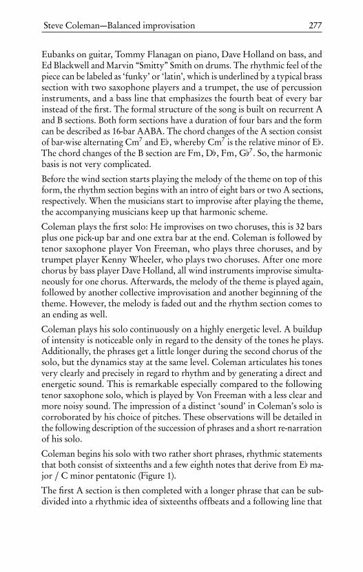
Steve Coleman—Balanced improvisation 277
Eubanks on guitar, Tommy Flanagan on piano, Dave Holland on bass, andEd Blackwell and Marvin “Smitty” Smith on drums. The rhythmic feel of thepiece can be labeled as ‘funky’ or ‘latin’, which is underlined by a typical brasssection with two saxophone players and a trumpet, the use of percussioninstruments, and a bass line that emphasizes the fourth beat of every barinstead of the first. The formal structure of the song is built on recurrent Aand B sections. Both form sections have a duration of four bars and the formcan be described as 16-bar AABA. The chord changes of the A section consistof bar-wise alternating Cm7 and E[, whereby Cm7 is the relative minor of E[.The chord changes of the B section are Fm, D[, Fm, G[7. So, the harmonicbasis is not very complicated.
Before the wind section starts playing the melody of the theme on top of thisform, the rhythm section begins with an intro of eight bars or two A sections,respectively. When the musicians start to improvise after playing the theme,the accompanying musicians keep up that harmonic scheme.
Coleman plays the first solo: He improvises on two choruses, this is 32 barsplus one pick-up bar and one extra bar at the end. Coleman is followed bytenor saxophone player Von Freeman, who plays three choruses, and bytrumpet player Kenny Wheeler, who plays two choruses. After one morechorus by bass player Dave Holland, all wind instruments improvise simulta-neously for one chorus. Afterwards, the melody of the theme is played again,followed by another collective improvisation and another beginning of thetheme. However, the melody is faded out and the rhythm section comes toan ending as well.
Coleman plays his solo continuously on a highly energetic level. A buildupof intensity is noticeable only in regard to the density of the tones he plays.Additionally, the phrases get a little longer during the second chorus of thesolo, but the dynamics stay at the same level. Coleman articulates his tonesvery clearly and precisely in regard to rhythm and by generating a direct andenergetic sound. This is remarkable especially compared to the followingtenor saxophone solo, which is played by Von Freeman with a less clear andmore noisy sound. The impression of a distinct ‘sound’ in Coleman’s solo iscorroborated by his choice of pitches. These observations will be detailed inthe following description of the succession of phrases and a short re-narrationof his solo.
Coleman begins his solo with two rather short phrases, rhythmic statementsthat both consist of sixteenths and a few eighth notes that derive from E[ma-jor / C minor pentatonic (Figure 1).
The first A section is then completed with a longer phrase that can be sub-divided into a rhythmic idea of sixteenths offbeats and a following line that
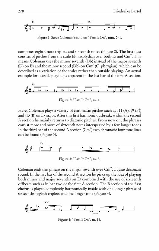
278 Friederike Bartel
Figure 1: Steve Coleman’s solo on “Pass It On”, mm. 0–1.
combines eighth-note triplets and sixteenth notes (Figure 2). The first ideaconsists of pitches from the scale E[mixolydian over both E[ and Cm7. Thismeans Coleman uses the minor seventh (Db) instead of the major seventh(D) on E[ and the minor second (Db) on Cm7 (C phrygian), which can bedescribed as a variation of the scales rather than outside playing. An actualexample for outside playing is apparent in the last bar of the first A section.
Figure 2: “Pass It On”, m. 4.
Here, Coleman plays a variety of chromatic pitches such as ]11 (A), ]9 (F])and [13 (B) on E[major. After this first harmonic outbreak, within the secondA section he mainly returns to diatonic pitches. From now on, the phrasesconsist more and more of sixteenth notes interspersed by a few longer tones.In the third bar of the second A section (Cm7) two chromatic four-tone linescan be found (Figure 3).
Figure 3: “Pass It On”, m. 7.
Coleman ends this phrase on the major seventh over Cm7, a quite dissonantsound. In the last bar of the second A section he picks up the idea of playingboth minor and major sevenths on E[ combined with the use of sixteenthoffbeats such as in bar two of the first A section. The B section of the firstchorus is played completely harmonically inside with one longer phrase ofsixteenths, eighth-triplets and one longer tone (Figure 4).
Figure 4: “Pass It On”, m. 14.
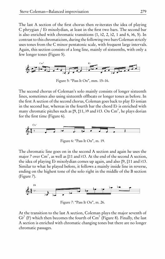
Steve Coleman—Balanced improvisation 279
The last A section of the first chorus then re-iterates the idea of playingC phrygian / E[ mixolydian, at least in the first two bars. The second baris also enriched with chromatic transitions (1, [2, 2, [2, 1 and 6, [6, 5). Incontrast to this chromaticism, during the following two bars Coleman strictlyuses tones from the C minor pentatonic scale, with frequent large intervals.Again, this section consists of a long line, mainly of sixteenths, with only afew longer tones (Figure 5).
Figure 5: “Pass It On”, mm. 15–16.
The second chorus of Coleman’s solo mainly consists of longer sixteenthlines, sometimes also using sixteenth offbeats or longer tones as before. Inthe first A section of the second chorus, Coleman goes back to play E[ ionianin the second bar, whereas in the fourth bar the chord E[ is enriched withmany chromatic pitches such as ]9, ]11, [9 and [13. On Cm7, he plays dorianfor the first time (Figure 6).
Figure 6: “Pass It On”, m. 19.
The chromatic line goes on in the second A section and again he uses themajor 7 over Cm7, as well as ]11 and [13. At the end of the second A section,the idea of playing E[mixolydian comes up again, and also ]9, ]11 and [13.Similar to what he played before, it follows a mainly inside line in reverse,ending on the highest tone of the solo right in the middle of the B section(Figure 7).
Figure 7: “Pass It On”, m. 26.
At the transition to the last A section, Coleman plays the major seventh ofG[7 (F) which then becomes the fourth of Cm7 (Figure 8). Finally, the lastA section is enriched with chromatic changing tones but there are no longerchromatic passages.

280 Friederike Bartel
Figure 8: “Pass It On”, m. 28.
Figure 9: Distribution of midlevel units (MLU) in “Pass It On”.
What is remarkable for the whole solo is Coleman’s alternation betweendiatonic and chromatic playing. He repeats certain ideas, such as playingE[mixolydian on E[ and on Cm7, which then becomes C phrygian. Rhyth-mically, the combination of mainly sixteenths with sixteenth offbeats andtriple eighths is notable. This examination of the solo provides a first impres-sion and exemplifies Coleman’s usage of chromatic pitches—which in turnpartly explains the ‘special’ sound of Coleman’s playing. In the following,some of these observations will be enriched and visualized by using tools ofthe MeloSpyGUI and by giving some examples for possible interpretationsaccording to the rules of Symmetrical Movement. Firstly, on examinationof the midlevel annotation (Figure 9, see for an explanation of midlevelunits), it is noticeable that there are only licks and lines, mostly wavy lines,as well as one void, but no units categorized as melody, rhythm, expressiveor as referring to the theme. This observation, in addition to the followinganalyses, confirms the title of this chapter, for Coleman’s playing seems to bemainly concerned with rhythmic and intervallic construction. By listeningto Coleman’s improvisations, one can get the impression that he builds up

Steve Coleman—Balanced improvisation 281
an area of tones by compounding certain constant rhythmic and harmonicparameters that follow certain rules. The constructive quality of Coleman’ssolo may be connected to his concept of Symmetrical Movement, whichactually consists of rules for choosing intervals while disregarding chords.Moreover, an ongoing rhythmic grid of sixteenths seems to be underlying hisimprovisation, like bricks that build the foundation of a building. However,a constant rhythmic grid is contrary to the idea of a rhythmically variedmelody.
Figure 10 (top left corner) shows the Metrical Circle Map of Coleman’s solo.All the tones are here assigned to 48 rhythmic positions within the 4
4-bar.The diagram visualizes the frequencies of the different rhythmic placementsused by Coleman. Very frequently, Coleman plays on- and offbeat positionsconcerning the eighth-grid (1, 1+, 2, 2+, 3, 3+, 4, 4+); they all occur between16 and 21 times. Also very frequently, he plays the sixteenth offbeats in be-tween all the aforementioned positions, whereas tones on sixteenth positionsbetween 3+ and 4, 4 and 4+, 4+ and 1 are as frequent as on eighth positions.So this diagram certainly gives an impression of Coleman’s balanced metricaltone placements. Another reference to the terms balance and symmetry isColeman’s preferred use of a binary rhythmic grid rather than a ternary one,as the diagram shows. Eighths and sixteenths form a grid with a symmetricbinary division of time intervals which is not possible within a ternary grid.Of course, in this case the rhythmic feel of the music is played in a binaryway, but Coleman also plays binary within a ternary rhythmic framework,which will be pointed out later.
The top left corner in Figure 11 pictures Coleman’s use of pitch classes withrespect to the particular chords played by the rhythm section in percent.The numbers one to seven represent the chord tones (1, 3, 5, 7) and tensions(2, 4, 6), and the numbers and letters on top of that represent the remainingtones that fill up the chromatic scale ([13 =minor sixth, [9 =minor ninth,]11= tritone, ]7=major seventh over minor seventh chord, ]9=minor thirdover major chord, ]10 =major third over minor chord, [7 =minor seventhover major seventh chord). The diagram shows that Coleman plays primarilydiatonic pitch classes while using all of the non-diatonic pitch classes more orless equally. He does not emphasize the chord tones in general, only the fifthand the seventh. Besides, he also uses non-diatonic pitch classes, but with amuch lower percentage. So in this case, balance does not mean that Colemanuses all twelve chromatic pitch classes equally often, as in, for example, twelve-tone music. This can also be demonstrated by the diagram in Figure 12 (topleft corner), which pictures all absolute pitches Coleman uses. With 45 times,B[4 is played by Coleman most often, followed by F4 and G4. All three tones

282 Friederike Bartel
Figure 10: Metrical Circle Maps of Steve Coleman’s, Kenny Wheeler’s, and VonFreeman’s solos on “Pass It On”, and Coleman’s and Wheeler’s solos on “Slippedagain”.
are consonant with Cm7 and E[, the chords of the A section that are playedmost of the time during the whole piece.
Figure 13 shows the alternating diatonic (or ‘inside’) and non-diatonic/chro-matic (or ‘outside’) character of successive phrases that were recognized in there-narration of the solo by picturing pitch classes in relation to the chord(s)within different phrases.
As described before, some phrases are completely diatonic, even pentatonic,such as phrases 2, 4 or 9 (phrase 1, the pick-up bar, is missing because, tech-nically, there was no chord annotation available). Three phrases (7, 8 and10) emphasize the [9 as an extra chromatic pitch. Finally, there are phrases

Steve Coleman—Balanced improvisation 283
Figure 11: Distribution of extended chordal diatonic pitch classes of Steve Cole-man’s, Kenny Wheeler’s, and Von Freeman’s solos on “Pass It On”, and Coleman andWheeler’s solos on “Slipped again”.
Von Freeman − Pass it On
Kenny Wheeler − Pass it on Kenny Wheeler − Slipped again
Steve Coleman − Pass it On Steve Coleman − Slipped again
C3 G3 C4 G4 C5 G5 C6 G6 C7
C3 G3 C4 G4 C5 G5 C6 G6 C7
0%
5%
10%
15%
0%
5%
10%
15%
0%
5%
10%
15%
Pitch
Per
cent
age
(%)
Figure 12: Distribution of pitches of Steve Coleman’s, Kenny Wheeler’s, and VonFreeman’s solos on “Pass It On”, and Coleman’s and Wheeler’s solos on “Slippedagain”.

284 Friederike Bartel
Figure 13: Phrase-wise distribution of extended chordal diatonic pitch classes ofSteve Coleman’s solos on “Pass It On”. Dark blue = ‘inside’ diatonic tones, lightblue = ‘outside’ non-diatonic tones.
Figure 14: Phrase-wise distribution of extended chordal diatonic pitch classes ofSteve Coleman’s solos on “Slipped again”. Dark blue = ‘inside’ diatonic tones, lightblue = ‘outside’ non-diatonic tones.

Steve Coleman—Balanced improvisation 285
Figure 15: Distribution of interval classes of Steve Coleman’s, Kenny Wheeler’s, andVon Freeman’s solos on “Pass It On”, and Coleman and Wheeler’s solos on “Slippedagain”.
that can be described as mainly chromatic, such as phrases 3, 5 or 11. Thealternation of diatonic and chromatic phrases is clearly visible. This could beinterpreted as a kind of balancing, which means that Coleman doesn’t usechromatic tones as a device for building up tension in the course of the solo,but instead starts with a chromatic line right away.
In Figure 15 (top left corner), one can see the percentage of interval classes:steps up and down, leaps (minor and major thirds) up and down, jumps(fourths, tritones, and fifths) up and down, and large jumps (sixths and larger)up and down. The distribution of interval classes can be approximatelydescribed as balanced, although Coleman plays slightly more ascending inter-vals than descending. However, this distribution cannot exactly capture theconcept of Symmetrical Movement, because it refers to particular cases inwhich tones should be played consecutively, not to the occurrence of certainintervals during an entire solo. This is why we will give two typical but rathershort examples from the solo.
The first example is taken from m. 10, which is the second bar of the firstB section. The eighth triplet on beat three includes the tones A[, B[, andG[. If A[ is considered to be the axis tone, B[ and G[ are equidistant fromthis axis, either a major second above or below. The same principle can bedetected for the tones B[, C, and G[ beginning on beat two of the same bar.

286 Friederike Bartel
Figure 16: Symmetric Movement example (“Pass It On”, m. 10).
The second example is part of a more chromatic passage of Coleman’s soloin m. 28. On beat three he plays E, F, and E[, the minor seventh, major
Figure 17: Symmetric Movement example (“Pass It On”, m. 28).
seventh and the 13th of the chord G[7 of the last B section. The symmetryhere follows the same structure as in the first example, only using minorseconds instead of major seconds. E can be considered the axis tone, followedby the minor second above, F, and the minor second below, E[. Especiallythe chromatic passages of the solo offer a good source for more examples likethis. There are examples of passages with larger intervals and with more toneswhich could be related the concept of Symmetric Balance, too. However, inmost cases, the relation has a rather speculative character.
Comparative analysis
In the preceding sections, Coleman’s style of improvisation was describedas individually shaped, originating from his sound, his choice of pitches andintervals, and his alternating usage of diatonic and chromatic pitches resultingin a characteristic style of exact rhythmic and advanced melodic playing. Thecharacterization of personal style can be regarded as one of the main aspectsof jazz research as well as highly important for the jazz musicians themselves,since improvisation in jazz involves personal expression and the developmentof a personal ‘sound’. To examine style, comparisons can be of further help.
The first possibility for a comparison is to take other musicians into account.For this case study, it is appropriate to look at the solos of Kenny Wheelerand Von Freeman on “Pass It On”. Additionally, Coleman’s solo on “PassIt On” will be compared to his improvisation on the blues “Slipped again”whose ternary rhythmic feel contrasts with the binary feel of “Pass It On”.“Slipped again” is a piece written by Coleman and recorded on Rhythm InMind (1991). The key is F and the form can be described as a standard bluesform enriched with a few II-V progressions. After a tenor saxophone solo by

Steve Coleman—Balanced improvisation 287
Von Freeman, a trumpet solo by Kenny Wheeler and a piano solo by TommyFlanagan, Coleman plays the fourth solo on this recorded version of thesong, followed by a bass solo by Dave Holland. Listening to the three solosof Coleman, Wheeler and Freeman, there are clear differences concerningsound, rhythmic attitude, energy, and choice of pitches.
Although the differences between the Metrical Circle Maps of Coleman’s,Wheeler’s and Freeman’s solos (Figure 10) are rather subtle, the distinctiverhythmical playing of Coleman is visibly accessible in “Slipped again”, too.Kenny Wheeler mainly emphasizes the downbeats and plays many tones inbetween the sixteenths, which can indicate a less rhythmically precise or afaster playing (the latter cannot be proved by listening). Freeman, on theother hand, emphasizes the eighth offbeats but not the sixteenth offbeats likeColeman and again, there are more counts in between the sixteenths.
The second comparative diagram (Figure 11) shows the different pitches thethree musicians use in their solos. Firstly, it represents the very different pitchranges, which are partly due to the different instruments being played: altosaxophone, trumpet and tenor saxophone. Wheeler on trumpet thereforeuses the highest tones and Freeman on tenor saxophone the lowest. Secondly,the diagram illustrates that Coleman and Wheeler both emphasize B[4 anda few other tones due to the changes of the A section, whereas Freemanplays very chromatically with nearly uniformly distributed pitches. Thiscorresponds to the listening impression.
To compare sound and dynamics by visualization, different methods wouldbe necessary, for example spectral analysis or other tools the MeloSpyGUIoffers. But the analysis so far already proves that many of the previouslyrecognized distinctive aspects of Coleman’s improvisational style cannot befound in the same way in the solos of Wheeler and Freeman. These are, forexample, a rhythmical exactness based on a clearly played sixteenth-grid andthe observation that the goal of reaching musical balance and the trainingof the Symmetrical Movement don’t lead to an entirely chromatic style ofplaying in Coleman’s solos. In fact, Freeman plays more chromatically thanColeman.
Listening to Coleman’s solo on “Slipped again” again gives the impressionthat he switches between blues scale / diatonic playing and outside playing.This is emphasized by a visualization of the pitch classes within the phrasesof the solo in Figure 14.
Besides the alternating diatonic and chromatic usage of pitches that wasalready recognized in Coleman’s solo on “Pass It On”, some further observa-tions are striking. For example, phrase 14 consists simply of the [9 and theroot of C7 followed by the third of the following chord Fm7. In contrast,

288 Friederike Bartel
in phrase 13, immediately beforehand, there are a variety of diatonic andchromatic pitches with more outside than inside pitches. Yet, this diagramsupports the assumption that Coleman uses an alternation of diatonic andchromatic phrases as a stylistic device.
What generates an easily interpreted graphic is the comparison of the MetricalCircle Map of Coleman’s solo in “Pass It On” with the one of his solo in“Slipped again” (Figure 7, top row). Arguably, both distributions do not lookentirely alike, but they clearly do give an approximative impression. Beatone and three are emphasized more in “Slipped again”, and the sixteenth gridis clearly evident. This observation is further supported if one looks at thecomparison between the Metrical Circle Map of Wheeler’s solo in “Slippedagain” and the one of Coleman’s solo (Figure 10, left column). Wheeleremphasizes beat one and four, comparable to how Coleman emphasizes beatone and three, but the sixteenth grid is much less visible in Wheeler’s solo,probably due to a more ternary style of playing.
All these comparisons underline personal distinctiveness in the improvisa-tional style of Coleman, and also in the styles of Wheeler and Freeman. Theexamination of stylistic aspects, which in this chapter was focused on rhyth-mic and harmonic parameters, could be expanded by additional stylisticallyrelevant features.
Conclusion
The aim of this case study was to analyze individual stylistic aspects of Cole-man’s improvisational style. After outlining Coleman’s musical heritage, wehad a closer look at one specific solo taken from “Pass It On”. Next, weobtained insights from comparative analyses of solos by Kenny Wheelerand Von Freeman on the same tune, on one hand, and of a second solo byColeman taken from the blues “Slipped again”, on the other hand.
The first step disproved the assumption that Coleman plays in a very chro-matic way by using all twelve tones equally, due to the melodic approachthat was derived from the concept of Symmetrical Movement. It was insteadconfirmed that Coleman combines intervallic symmetry with the harmoniccontext of the song rather than ignoring the chord-scale theory altogether,but also that he uses the alternation of inside and outside playing as a stylisticdevice. Likewise, it came to light that the symmetry he approves in his essaycan also be found in prevalent binary subdivisions of the beats, as well as in arhythmically exact playing.
To make sure that these results of the stylistic analysis are distinctive ratherthan general occurrences in jazz improvisation, comparisons were made in

Steve Coleman—Balanced improvisation 289
a second step. The comparative diagrams based on the solos of Wheeler,Freeman and Coleman in the song “Pass It On” result in the findings thatneither Wheeler nor Freeman play rhythmically inside a sixteenth grid asColeman does. This corroborates the assumption that this is an aspect of hisindividual style.
Finally, the comparison of the first analyzed solo of Coleman in “Pass It On”with his solo in “Slipped again”, which are both part of the record RhythmIn Mind, again proved the previously made assumptions, e. g., his switchingbetween inside (blues scale) playing and outside passages. As the SymmetricalMovement concept is hard to fully reconstruct, it can only be assumed thatthe thoughts that go along with it and the training of the intervallic structureslead to the idea of alternating diatonic and chromatic passages, especially inlight of Coleman’s statement that strictly adhering to either the SymmetricalMovement approach or the chord-scale approach would be equally ‘boring’.
Further possibilities for examining Coleman’s style would be, for example, inadditional timbral studies. Another option would be to analyze the individualphrases or more solos in more detail. In this way, one could draw additionalconclusions about how Coleman builds up his improvisations, especiallyabout how fundamental the alternation of inside and outside playing is forhis personal style, or how he uses rhythm and certain motives to build uphis solos. Possibly, the terms of symmetry and balance might come up again.


Following the red line: Chris Potter’s solo on“Pop Tune #1”
Wolf-Georg Zaddach
A world-class soloist, accomplished composer and formidablebandleader, saxophonist Chris Potter has emerged as a leadinglight of his generation. Down Beat called him ‘one of the moststudied (and copied) saxophonists on the planet’ while Jazz Timesidentified him as ‘a figure of international renown.’ Jazz saxelder statesman Dave Liebman called him simply ‘one of the bestmusicians around,’ a sentiment shared by the readers of DownBeat in voting him second only to tenor sax great Sonny Rollinsin the magazine’s 2008 Readers Poll (Milkowski, 2017).
Going by his biographical article on the saxophonist’s homepage, journalistand producer Bill Milkowski is undoubtedly convinced by Potter’s accom-plishments. By 2017, Potter had recorded 19 albums as a leader and appearedon over 100 albums as a sideman. The list of musicians he worked with readsas a Who’s Who of the recent and contemporary American jazz scene: PaulMotian, Dave Holland, Herbie Hancock, John Scofield, Jim Hall, Dave Dou-glas, and many more. Potter, born in Chicago, Illinois in 1971 and raised inColumbia, South Carolina, has been part of the New York City scene since1989, when he started studying at the age of 18 and played in the band of RedRodney, who himself had played alongside Charlie Parker. While Milkowskidescribes Potter’s output in superlatives emphasizing the musician’s interna-tional success, the attraction of his playing may be rooted in his awarenessand mastery of the tradition as well as of contemporary jazz:
My aesthetic as a saxophonist has always been based in Bird andLester Young and Sonny Rollins and all the other greats on the

292 Wolf-Georg Zaddach
instrument. What I’ve learned from them in terms of phrasing,sound, and approach to rhythm I’ll never outgrow,
Potter stated, as cited by Milkowski (2017). Nevertheless, even with his solorecordings, Potter displays a diversity that spans from postbop to moderngroove and fusion. In fact, Potter shows an openness for diverse musicalgenres, and reflects artistically on the music he grew up with:
I’ve been touched by many forms of music, like funk, hip hop,country, different folk musics, classical music, etc., and for menot to allow these influences into my music would be unneces-sarily self-limiting. The difficulty is incorporating these soundsin an organic, unforced way. It helps me to remember I wantpeople to feel the music, even be able to dance, and not think ofit as complicated or forbidding (Milkowski, 2017).
His band project Chris Potter’s Underground is such an attempt to explorecontemporary sounding, groove-based, and rhythmically challenging music.In a setup that includes a modern-sounding electric guitar (Wayne Krantz,later Adam Rogers), a Fender Rhodes (Craig Taborn) that also takes overthe function of the bass, and drums (Nate Smith), Potter can connect hiseducation and experience as a postbop saxophonist with groove and funk-oriented music. Since Potter has proved his postbop playing abilities manytimes with recordings such as Presenting Chris Potter (1992), Unspoken (1997),or recently The Dreamer Is the Dream (2017), it seems worthwhile to analyzehis improvisation in a groove context. In the following, I will discuss thesolo on “Pop Tune #1” on Follow the Red Line: Live at the Village Vanguard,recorded during a three-night appearance from February 15th and 17th 2007in New York City. At this point, Potter had already been experimentingwith this line-up and aesthetic for several years and had released a first stu-dio recording with the highly acclaimed album Underground in 2006. Oneperspective on the music of Potter’s Underground could be that it unitesfunk and groove rhythms and aesthetics with the inventiveness and rhythmic,as well as melodic, versatility of postbop improvisation. “It’s an exercise infutility to find a name for the music of Follow the Red Line”, emphasizes JohnKelman in a review of the album. He further states that Potter convincingly
[. . . ] blurs the lines between jazz, rock, funk and even a little afro-beat in ways that are finally being accepted again two decadesafter The New York Times declared the ‘pestilence known asfusion is dead,’ the best word to describe this recording is, quitesimply, great (Kelman, 2007).

Chris Potter’s solo on “Pop Tune #1” 293
While Kelman is speaking about the music in general, an interesting questionis: Does Potter blur the lines during his improvisation, too? And if so, howdoes he adjust and develop his improvisation in the groove context?
Following the red line: the overall structureof the performance and solo
The hybridization of postbop and modern pop/rock styles is at the core ofFollow the Red Line. At first sight, most of the tracks follow the conventionalstructure of postbop music with an introduction, a (sometimes complex)head, solos, and the head again. “Pop Tune #1” is slightly different though.The performance is split into two main parts. The first part (0:00–6:30 min)has a medium slow tempo in a 6
8-meter, emphasizing a ballad feeling with aconstant harmonic rhythm, slightly shifting through different harmonic cen-ters. During the first part, guitarist Adam Rogers plays an intense solo with arepetition of the head at the end. Then, Chris Potter starts an unaccompaniedinterlude to the second part of the performance (6:30–7:03 min). Followingthis, Potter improvises for another four and a half minutes, accompaniedby the band. The solo culminates in a theme-like passage and ends ratherunexpected (11:01–11:38 min). Potter’s interlude and solo during the secondpart will be in the focus of the following analysis.
Setting the groove—Potter’s solo interlude
The first main part, at approx. 102 bpm and in a 68-feeling, ends with a slight
collective rubato during the last measure and a stop on beat one of the nextmeasure, followed by a slow fade-out by the guitar and keys. Potter uses thestop as a starting point for his improvisation. However, he does not startwith the band’s emphasis on beat one, but instead installs a new time feelingand meter starting on the next beat. What follows is an improvised 30-secondsolo of 16 measures without the band, functioning as an interlude to thesecond part of the performance (see Figure 1). Potter plays in a groovy 4
4-feeling, emphasizing the beats and off-beats with short, accentuated tones anda harmonically rather stable, static tonal center on G, based on the last chordof part one (Gm). The tempo is marginally faster with approx. 108 bpm, andPotter shifts slightly during his solo interlude. While he starts the phraseson the off-beats, he stabilizes the time feel and meter with the percussivenoise of pressing down lower keys without an air stream on the saxophone.However, it is the contrast of accentuation and phrasing as well as the switch
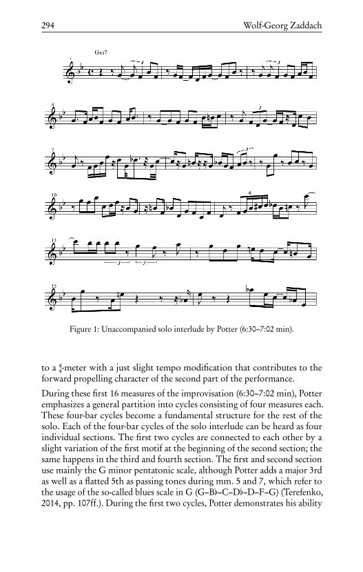
294 Wolf-Georg Zaddach
Figure 1: Unaccompanied solo interlude by Potter (6:30–7:02 min).
to a 44-meter with a just slight tempo modification that contributes to the
forward propelling character of the second part of the performance.
During these first 16 measures of the improvisation (6:30–7:02 min), Potteremphasizes a general partition into cycles consisting of four measures each.These four-bar cycles become a fundamental structure for the rest of thesolo. Each of the four-bar cycles of the solo interlude can be heard as fourindividual sections. The first two cycles are connected to each other by aslight variation of the first motif at the beginning of the second section; thesame happens in the third and fourth section. The first and second sectionuse mainly the G minor pentatonic scale, although Potter adds a major 3rdas well as a flatted 5th as passing tones during mm. 5 and 7, which refer tothe usage of the so-called blues scale in G (G–B[–C–D[–D–F–G) (Terefenko,2014, pp. 107ff.). During the first two cycles, Potter demonstrates his ability

Chris Potter’s solo on “Pop Tune #1” 295
to develop short and rhythmic motifs which create a certain groove feeling.In fact, the first four measures can be split into three phrases: the introductionof a spontaneous motif in m. 1, which emphasizes the root G and picks upthe tonality of the band’s playing before the interlude. By starting the phrasein between beats two and three and by placing the other intervals on beatfour, Potter creates a certain rhythmic tension due to the new time feel andmeter. In measure two, Potter varies the motif, starting with a prelude to themotif between beats one and two, though the G is again placed between beatstwo and three. The end of the motif is reduced, the F is left out. In measurethree and four, Potter plays a fusion of the two previous ideas: The preludebecomes part of the new motif. The G, until now placed on the offbeat,is now placed on beat three, which gives the whole motif a rather stablecharacter. He repeats this variation of motif 1 twice, varying the ending. Bothimportant tones, the G and the following B[ are repeated now on strong beatswith a slightly laid-back feeling. That slight variation in rhythmic placementas well as the limitation to certain repeated tones already prepares the wayfor the groove feeling to be established by the band.
During mm. 5 to 8, Potter works with the first motif again, varying it in anew way. Sticking with the idea of starting the phrase on the offbeat betweenbeats one and two, he especially mirrors the ending of that motif. Insteadof leaping down from the B[ to the F, he steps up chromatically to the C byadding the major third B (m. 5). By incorporating tones above the B[ for thefirst time, he expands his flow of motivic development in a coherent way. Thenext phrase in m. 6 picks up the idea of preluding the motif again, followedby mirroring the ascending G–B[–C in m. 5 into a descending C–B[–G andplacing the G on the strong beat one of m. 7, which gives it a certain cadentialcharacter. Without a break, he continues to emphasize tones that are built upby a descending line which has a bluesy guide-tone line character (D–D[–C–B–B[) as well as a cadential character, too (m. 8). Interestingly, this could be apoint where the band enters: So far, Potter has played eight measures and acadence-like motif at the end of it. Yet Potter leaves the cadence somehowunfulfilled by stopping right between beats three and four, resting on beatfour to the next beat one.
The following eight measures work with new motifs and yet are connectedto the first eight measures through the usage of and in reference to theG blue scale and the rhythmic placement of accents on beat three as wellas on offbeats (mm. 9, 12, 13, 15). In m. 11, he plays natural fourths thatleap up but are incorporated in a descending melodic line (G–F–D–C) whichgives this part a somehow jumpy, excited feeling (m. 11). During the last fourmeasures, he varies this idea with a rather clear cadence: First he expandsthe heavily blues-influenced harmonic frame with a descending line that im-
296 Wolf-Georg Zaddach
plies a C major pentatonic (G–E–D–C). This is followed by a chromaticallydescending line (F–E–E[) varying the motif of fourths into leaps of fifths(mm. 15 and 16). After the A[ in m. 16, he plays an A[ arpeggio which couldfunction as a form of cadential closure, interpretable as a tritone substitutionof the dominant D or simply a side-stepping from the tonic G turned intomajor.
At this point, Smith and Taborn enter (7:02 min). They start with hesitantaccents on the Fender Rhodes, limited to the higher registers, and quiet rimclicks on the snare drum. They keep the energy low and leave room forthe music to grow gradually. In m. 19, a high level of interplay becomesobvious: After the band has entered, Potter stops to play for one and a halfmeasures. Then, he offers a phrase that emphasizes the offbeats with shortand concise accents followed by a series of accents on the beats starting withbeat two of m. 19. Nate Smith reacts immediately and keeps emphasizingevery beat with his bass drum and off-beat accents on the hi-hat. Potter andSmith repeat these accents synchronously for several beats. This spontaneousrhythmic loop enables Smith to stick to a certain groove pattern while stillkeeping the volume level low. For the rest of the solo, Smith maintains thispattern of a four-to-the-floor disco groove on the bass drum and offbeatphrasing on the hi-hat. After four measures, he adds rim clicks on the snareon beats two and four. At the same time, Taborn starts to play a G in thelow register of the Fender Rhodes on beat one of every second measure. Itis part of this line-up without a string bass that may enable the feeling andrepetition of groove cycles in a certain way: The lower registers of a FenderRhodes are less prominently audible than the attack of a plucked string bass,therefore lower keys require a strong attack in order to be heard as bass tones,a constant bass line would thus require a lot of muscle strength. However,these strong accents in the lower registers with a certain amount of spacein between permit the creation of certain patterns of groove in the contextof four-bar cycles as Taborn does. Choosing these regular cycles follows theregular structure of Potter’s interlude and yet leaves the opportunity openfor developing rather complex rhythmic patterns in the frame of four-barcycles, e. g., with cross- or superimposed rhythms.
After another four-bar cycle, Adam Rogers adds a funky guitar pattern thatat the same time emphasizes the tonal center G and picks up Potter’s bluesimplications during the interlude by sliding into the minor third and fifthof the G minor triad from below. The development of the accompanimentchanges in intensity and small chord variations and provides a fundamentalgroove for another two minutes.

Chris Potter’s solo on “Pop Tune #1” 297
After about two minutes of Potter’s solo, Taborn and Rogers split the four-bar cycle harmonically into two parts, beginning in m. 85: Two measures ofG minor, occasionally played as G major, are followed by a shift to B[minor,accompanied by a switch to the full snare hit on beats two and four. Theharmonic rhythm emphasizes the four-bar cycles as well. This section func-tions as a second part of the solo. The cue happens after exactly 17 four-barcycles. During this second part of his solo, Potter improvises over another10 four-bar cycles, followed by a theme-like motif in the high register thatspans over four measures and is repeated three times, so that the tune endswith four four-bar cycles—the same length as the interlude at the beginningof Potter’s solo.
Distinct features of Potter’s solo
As shown, rhythmic motifs especially supporting the strong beats and offbeatsare important features since the start of the solo. During his improvisation,Potter balances out complex and fast lines with rhythmic motifs that supportthe groove established by the drums, Fender Rhodes and guitar. Further,the unaccompanied solo interlude functions as a reference: After the bandenters, Potter improvises over two four-bar cycles before he starts repeatingthe theme-like motif from m. 1 with just a slight variation (mm. 25–28).He contrasts this reminiscence of the beginning of his solo with fast playedlines that rise and fall in wave-like contours and span over a length of twomeasures (mm. 30–41). He mainly uses tones of the G dorian scale, with slightdeviations by playing arpeggios that imply a C13 (m. 31) and G7]5 (m. 32). Inm. 34, he ends a longer line which quotes the distinct motif of m. 1 with itsfalling interval on beat three.25
In m. 39, he begins to introduce another feature of the solo: highly chromaticlines with mainly descending contours. However, Potter organizes these byplaying with short ascending motifs of three- or two-tone cells (Figure 2).
Figure 2: Chromatic motif in mm. 39f., starting with an ascending three-tone cellfollowed by an ascending two-tone cell, built into a line with a descending contour.
25Potter keeps quoting this motif, e.g. in m. 54.

298 Wolf-Georg Zaddach
He frequently gets back to this idea of chromatic descending lines with a clearreference to m. 39 and 40 (Figure 2): in m. 42 and mm. 43f., with variationsand extensions in mm. 99ff. He also repeats the idea of two- or three-tonecells, e. g., in m. 56 with tonal material inside the harmonic frame. M. 51displays a certain variation of this idea: Here, Potter varies the idea of two-tone cells by mirroring and expanding the cell-idea to a sequence of four-tonepatterns (Figure 3). He starts with the mirrored cell, so that there is a stepdownwards by a second. This is answered by the original two-tone cell witha leap upwards by a second so that it expands to a four-tone pattern. The twomotifs are connected by a large jump downwards, first by a minor sixth, thenby a perfect fifth, a tritone and a minor sixth again. Each four-tone patternuses tones outside the harmonic center of G. Played in a sequence, the patternfollows the logic of outside-playing called ‘constant structure’, although theinterval structure of the pattern itself is not repeated exactly.
Figure 3: Sequence of four-tone patterns as a motivic variation and extension ofprevious two-tone cells.
Figure 4: Ascending constant structure of arpeggios (root, fifth, octave) starting onB[–C–E[–F–G[, illustrated by brackets. The arpeggios are played in a wavy contour,however the overall contour with its different roots is ascending.
In mm. 70 and 71, Potter plays a sequence of patterns of upward jumps of afifth followed by a fourth up and a fourth down. He starts on a B[ and repeatsthat exact interval pattern starting on the tone C, then E[, F, with additionalembellishments to the fifth, and G[ (Figure 4). This stack of fourths and fifths

Chris Potter’s solo on “Pop Tune #1” 299
creates another constant structure of a four-tone pattern. Each arpeggio spansover an octave and contains the root, fifth, and octave, e. g., B[3–F3–B[4–F3.Due to the rhythmic placement and the speed of the line, the starting tones donot fall on the beats, so that the overall contour consists of wide oscillationsover an ascending line.
The fast and complex outside lines are balanced out by harmonically insideand rhythmically clear and rather simple passages. For example, in m. 66,Potter starts with such a passage, which he varies slightly in regard to rhythm(Figure 5). The rather simple character is provided by tone repetition anda rhythmic template of quarter and eighth notes. After the previous densephrases, this offers a moment of release and supports the groove.
Figure 5: Rhythmic motif with tone repetition and slight rhythmic variations (m. 66–69).
The beginning of the second part of the solo is strongly supported by arhythmically accentuated passage in mm. 85ff. (Figure 6). Here, Potter plays arhythmic figure of a dotted quarter note and an eighth note, simply alternatinga G and a B[. Due to its rhythmic and melodic structure, it could be heard as areference to the solo interlude. However, the funky groove is supported hereby rhythmic placements on the beats one and three. Potter reacts to the newchord progression played by Taborn and Rogers immediately. Already at thefirst appearance of the B[m7 in m. 87 he plays the corresponding triad withthe tones F–B[–D[. In the following measure, he clearly plays the B[minorpentatonic.
Figure 6: Rhythmic motif emphasizing beat one and three at the beginning of thesecond part of the solo (mm. 85ff.).

300 Wolf-Georg Zaddach
Pitch range Chromaticism
Event density Mean pitch
0 10 20 30 0 10 20 30
55
60
65
70
75
0.0
0.1
0.2
0.3
0.4
2
4
6
8
10
10
20
30
40
Measure number
Figure 7: Event density (tones per second), mean pitch (averaged across all MIDIpitches), pitch range (difference between highest and lowest pitch), and chromaticism(percentage of non-diatonic tones) over four-bar segments.
For the rest of the solo, Potter improvises over the chord progression ofGm7 and B[m7 and makes use of high chromaticism and techniques such asside-stepping (m. 95) and constant structure, e. g., of two-tone cells shiftedchromatically (m. 114f.). The last 16 measures have the character of a themeagain. Potter plays a rhythmically rather simple melody with a characteristicleap up of an octave over the Gm7 and a twelfth to the B[ over the B[m7. Herepeats this motif, which spans over four measures, three times with slightembellishments. The performance ends with a collective stop on the offbeatof beat four in m. 140.
Observations on dramaturgy and the choice of pitches
Up until its theme-like ending, Potter’s solo can be described as a discon-tinuous but still gradual intensification with frequent contrasting passages,supported by the band as well (Figure 7). The event density is at its lowestat the beginning (solo interlude) and at the end (theme-like motif with rep-etition). In between, Potter intensifies his phrases in general, yet varies theintensity a lot. What is remarkable is that Potter tends to avoid maintainingthe event density between the four-bar cycles. However, this is also due toPotter’s placement of the phrases. On the one hand, he connects almost

Chris Potter’s solo on “Pop Tune #1” 301
Figure 8: Pitch class distribution over phrase beginnings and endings and withinphrases (845 tones in 37 phrases).
all four-bar cycles by playing over the bar-line and ending a phrase at thebeginning of the next four-bar cycle. On the other hand, he rests frequentlyin between the cycles, several times for more than three beats. Due to this,the event density differs from four-bar cycle to four-bar cycle.
A similar observation can be made for the pitch range of every cycle—again,variability and contrast are important aspects for Potter’s solo. The mostobvious feature of the intensified dramaturgy is the mean pitch: By varyingthe register and the choice of pitches, Potter creates audible contrasts betweenthe four-bar cycles. Yet the mean pitch rises continuously, with the theme-likeending as one of the highest passages of the solo. The mean pitch rises overone and a half octaves between the beginning and the end.
As described earlier, chromaticism and outside playing are also importantfeatures of Potter’s solo. Interestingly, Potter plays phrases which are notchromatic at all (e. g., repetition of chord tones, see Figure 5), contrasted byphrases of high chromaticism. It is a distinct feature of the solo that it offersa pronounced contrast between inside and outside tones. Yet even the highlychromatic lines are not completely outside. In more than 80 % of the cases,the ending tones of the phrases are either a G, B[, D or F, and therefore insidethe underlying Gm7 (Figure 8). The C occurs as often as the D but can beunderstood as the eleventh and therefore a typical inside upper structureextension for minor chords. The beginnings of the phrases are mostly Gs and

302 Wolf-Georg Zaddach
Fs. Potter also starts frequently with an E or D] as a chromatic approach orembellishment, which adds a dorian character to the underlying Gm7. Thetonal material within the phrases is dominated by the tones G, B[, C, and F,which implies the relevance of the G minor pentatonic. By choosing tonalmaterial inside the harmonic frame with a strong emphasis on the G minorpentatonic at the beginnings, endings as well as within the phrases Pottercontributes to the less chromatic funk and pop/rock idiom with a static tonalcenter.
Conclusion
“Pop Tune #1” is one of several revealing testimonials to Chris Potter’s musi-cal flexibility and diversity. In the course of the solo, which spans over fourminutes, he combines techniques of postbop improvisation within the 4
4-funkgroove and a static tonal center. During his unaccompanied solo interlude,Potter displays his ability to set a new groove feeling and tempo with simplebut effective techniques, e. g., offbeat phrasing and accentuation. In the fol-lowing, he develops his improvisation by using techniques of self-quoting,motivic variation and tonal sequences spiced with a high amount of chromati-cism. Especially the latter is the result of postbop improvisation techniquesof outside playing and installing constant structures, among others. Yet heembeds these techniques in the musical context of a funk groove by contextu-alizing his playing in four-bar cycles, emphasizing offbeats and working withrhythmic motifs that support the groove. By doing so, he creates a playfulapproach to the funk groove—a red line leading through the track.

Head out


Conclusion and outlook
Martin Pfleiderer
The Jazzomat Research Project takes up the challenge of jazz research in theage of digitalization. It intends to open up a new field of analytical explo-ration by providing computational tools as well as a comprehensive corpus ofimprovisations with MeloSpyGUI and the Weimar Jazz Database. Followinga philosophy of open source, both the solo corpus and the software tools areopen for third-party additions and further development. The project aims atinitiating collaboration between researchers within the jazz research commu-nity as well as researchers from various other fields of research, in particularethnomusicology, music psychology, and music information retrieval.
How does the computational approach to jazz analysis contribute to jazz research?
This volume presents the concepts and approaches of the ongoing JazzomatResearch Project. Several case studies demonstrate how these concepts canbe included in jazz analysis to a varying extent and in different ways. Ingeneral, we propose to combine several methods of analysis. A combinationof close readings of single improvisations, comparisons, and distant readingsof big data corpora could contribute both to a data-rich history of jazz im-provisation and a better understanding of the psychology of improvisation.Most of the case studies within the second part of this book start with aclose description of single improvisations of an artist followed by either astatistical description of global stylistic features or the dramaturgy of a solo(e. g., Bob Berg, Miles Davis) or are dedicated to more specific research ques-tions such as a comparisons with other improvisations and improvisers (DonByas, Miles Davis, West Coast jazz, Freddie Hubbard/Woody Shaw, SteveColeman). For example, Don Byas’s solo on “Body and Soul” is comparedwith Hawkins’s famous solo on the same song, and Miles Davis’s solo on“Airegin” is contrasted to solos by other bebop trumpet players. Some studies,e. g., of Michael Brecker, Branford Marsalis, and Chris Potter, complement

306 Martin Pfleiderer
their analytical readings of single solos with certain computational and sta-tistical descriptions. Other chapters aim directly at proving or disprovinghypotheses on the improvisational styles of jazz musicians using computa-tional and statistical tools. In doing so, one crucial step is to decide whichcomputational features are particularly well suited. The broad scope of thecase studies included here shows that there is no single definite way to usethe Weimar Jazz Database and the accompanying analysis software. On thecontrary, it is up to the creativity of the researcher to use the possibilities ourdata and tools offer.
Generally, several musical domains could benefit from complementary sta-tistical approaches. Firstly, they allow both pinning down exact values andfrequencies and carrying out statistical tests and modeling, e. g., classificationand other machine learning methods. Secondly, pattern usage in a solo or acorpus, which is a central issue for research on improvisation, can be exam-ined using the pattern mining tools of the software. This opens up an area ofresearch on personal style and transmission of musical knowledge within thejazz community as well as on the cognitive foundations of improvisationalprocesses. Last but not least, these issues could be further examined by usingthe new approach of midlevel annotation that allows to distinguish betweenseveral playing ideas which are employed consciously or unconsciously bythe musicians.
Are there any specific results that are new and go beyond the findings of previousanalytical approaches?
Firstly, there are several clarifications and revisions of previous findings fromjazz research. For example, the intensification of Hawkins’s solo on “Bodyand Soul” described by Gunther Schuller is revisited and reformulated. Thefeatures that characterize both Miles Davis’s personal style of improvisationand the dramaturgy of his solos are examined in detail and contrasted with so-los of several bebop trumpet players. The analysis of Davis’s solo on “Airegin”shows that the midlevel approach in particular appears to be highly suitablefor analyzing jazz improvisations that lack virtuoso parts and instead focuson motivic inventiveness. The ‘lyricism’ attributed to the improvisationsof West Coast musicians Paul Desmond and Chet Baker is tied to certainmusical features and compared with solos of other cool and West Coast jazzmusicians. Several statistical results make it clear that Desmond and Baker, interms of tonal and rhythmic details, do not seem to be directly comparableto other musicians generally associated with cool jazz. All these findingspoint towards the importance of an identification of those musical featuresthat contribute to the overall listening impression of a certain improvisation.Statistical tools could contribute to solving the task of finding the musical

Conclusion and outlook 307
sources for certain stylistic attributions—which are sometimes associated ina rather vague manner. This includes dimensions such as pattern usage anddistribution of midlevel units both of which contribute to the dramaturgyand stylistic coherence of a jazz solo.
Six out of nine case studies focus on improvisations by postbop musicians.While the first half of jazz history is well documented and investigated, thesecond half of its history, starting around 1970, has not received sufficientattention so far. The personal styles of Freddie Hubbard and Woody Shaw arecompared, with a focus on specific improvisational details: fast tone chains,intervallic playing, and the usage of long patterns. While Hubbard and Shawappear to be highly comparable at first sight, the results show that theirpersonal styles, in part, distinctly differ, especially regarding the usage ofwide intervals in virtuoso lines and the playing of long interval and pitch pat-terns. The close analytical descriptions of solos by Michael Brecker, BranfordMarsalis and Chris Potter point towards innovative strategies for harmonicand rhythmic playing as well as their vital connection to the jazz tradition.Furthermore, it is demonstrated how the distinctive style of Steve Colemanin regard to melody and rhythm could partly be related to his idiosyncraticsystem of a ‘balanced’ or ‘symmetrical’ approach to improvisation. Probably,the case study on Bob Berg’s “Angles” goes furthest in an analytical attemptto reconstruct the formative creative strategies of Berg by analyzing his im-provisation in regard to several musical features and dimensions, patternusage, line construction, and overall dramaturgy.
Additionally, first promising results of using new analytical approaches arepresented within the first part of the book. The approach of an automatedfeature selection enables the identification of those statistically significantfeatures that distinguish certain subsets of improvisations, e. g., the personalstyle of one jazz musician compared to all other improvisations within thedatabase, to the characteristics of a certain instrument type, or to the impro-visations of a certain jazz style. For the first time, relations between harmonyand pitch choices within walking bass lines could be investigated on a broadbasis using the automatic transcription of bass lines due to an innovativetranscription algorithm. A novel algorithm framework for score-informedaudio analysis allows us to obtain new insights into expressive properties ofsolo improvisation such as intonation and the use of pitch modulation tech-niques and dynamics. As an initial approach to a description of the ‘sound’ ofjazz musicians, several timbre attributes were determined automatically andused to classify the performer of a given jazz solo recording using machinelearning techniques.

308 Martin Pfleiderer
The Weimar Jazz Database has only a limited corpus of transcriptions in a specialdata format. Does this restrict its usage for analytical research?
The limitation of a given data corpus is often a problem for statistical andcomparative approaches as well as for corpus studies in general. However,we think that the current version of the Weimar Jazz Database gives a moreor less representative overview of improvisation within the US jazz canon.Nonetheless, extensions and enhancements are always welcome. Therefore,we have published a short manual for the transcription of new material withthe aid of Sonic Visualiser software and with instructions for the correct dataformat. Following these instructions, anyone can contribute new transcrip-tions to the Weimar Jazz Database. Furthermore, the explicit data formatenables comparisons with other music corpora according to a number ofresearch questions, e. g., the degree of syncopicity or the prevalent melodiccontours of jazz lines contrasted to melodies in popular music or folk music.
While the transcriptions within the Weimar Jazz Database have been care-fully cross-checked several times, they are unfortunately not free of errors.However, the error rate seems to be very low with only a small impact onstatistical explorations. The data format was specifically designed to allowfor different directions of research, i.e., for the analysis of syntactical fea-tures of a solo on different levels of resolution, from the single-note levelto higher levels such as midlevel units, but also for more analysis aiming atperformance features such as micro-timing and tone formation. Fundamentalto this approach is the realization that there is no best solution when it comesto choosing a representation system or data format for music. Instead, musicrepresentations should be open to different functions and analytical applica-tions, e. g., for re-performances or, in our case, for analytical investigationsaccording to several—sometimes conflicting—research issues, as for examplein the interplay of micro-timing and syncopicity (Frieler & Pfleiderer, 2017).
Moreover, the data within the Weimar Jazz Database could serve as a groundtruth for various MIR tasks especially in regard to the development of in-novative algorithms for automatic transcription, annotation, and featureextraction from audio files, as well as for classification tasks. As an exam-ple, automatic melody transcription algorithms aim to group a given solorecording into a sequence of tone events with a discrete pitch, onset time,and duration. However, jazz artists frequently use dynamics and pitch modu-lation techniques such as vibrato or glissandi as an expressive means to alterthe pitch and intensity contours of tones, which significantly complicatesthe transcription task. Hence, the Weimar Jazz Dataset provides a valuabledataset with ground truth for melody annotations and can stimulate furtherresearch in this field.
Conclusion and outlook 309
What are the strengths and weaknesses of the software tools MeloSpyGUI andMeloSpySuite?
In developing the software, we aimed at balancing several criteria: On theone hand, the software should be powerful in covering many aspects anddimensions of melody within the context of jazz improvisation and beyond.On the other hand, it should be intuitive and easy to handle. However, themore functions are included in a software, the higher the risks of loss ofusability due to the broad range of possibilities. Moreover, in line with thephilosophy of open source and research collaboration, the software shouldbe open to enhancements and further developments. This affords a clear butopen concept that allows for extensions by others. We faced these challengesby providing extensive and detailed documentation of the software, withonline tutorials as well as several exemplary studies published in journals andproceedings and, last but not least, by publishing this project report.
The main benefits of the software tools are a fast and reliable processing ofqueries in regard to several musical parameters as well as to pattern usage andmidlevel units with a flexible selection of jazz improvisations (or parts ofthem). There are many features implemented in the software which meet thespecific demands of jazz research, e. g., to analyze pitch classes as a functionof the accompanying chords (e. g., chordal diatonic pitch classes and extendedchordal diatonic pitch classes), swing ratio (micro-timing), or statistical valuesfor syncopicity and the run-length of ascending, descending or chromaticphrases, and many more. This allows for investigations into stylistic featuresof jazz improvisation, commonalities and differences between different musi-cians or groups of musicians, into the development of those features over time,into pattern usage and into countless other research issues. The applicationsare not restricted to jazz improvisation but can be extended to many otherareas of musical melody—-provided that the melody repertoires are availablein one of the usable data formats. Unfortunately, many of the results aregiven in a data format (spreadsheets with comma separated variables) whichrequires further processing for exploration and visualization. The main newfeature in the upcoming version of the software is to include harmonic con-cepts of jazz theory which will allow for automatically relating tone sets, asplayed within phrases or sections, to a harmonic interpretation.
Can sound and timbre, group interaction and other performance qualities betaken into account, too?
Of course, the melodic lines improvised by jazz musicians are only one,albeit very important, aspect of improvisation. Sound, micro-rhythm, andgroup interaction are indispensable components of jazz performances too,
310 Martin Pfleiderer
and account for much of the enjoyment jazz listeners experience. In theJazzomat Research Project so far, we focused on the melodic and rhythmicalaspects of jazz improvisation. However, we also indicate new and forthcomingpossibilities of including such information as dynamics, intonation, micro-rhythm, or timbre. Information in respect to dynamics and intonation aswell as to micro-rhythm is already included in the Weimar Jazz Databaseand ready to be explored. The aspect of timbre or ‘sound’ seems to be morecomplicated, for conceptual as well as computational reasons, but first andpromising steps are made in regard to a comparison between the timbres ofdifferent jazz musicians.
In regard to group interaction, we have undertaken first attempts to includedata of the respective accompanying bass player. The automatically tran-scribed walking bass lines accompanying most of the solos are already in-cluded within the Weimar Jazz Database. Besides examining stylistic traitsof walking bass lines by different bassists, one could examine the relationbetween pitch choices of the soloists and those of the bass player. Theseobservations could lead to hypotheses relating to the mutual exchange ofplaying ideas in regard to harmony and contour. Another case is the rhythmicinteraction between the drummer and the soloist, especially between themicro-rhythm of the ride cymbal figure and the micro-rhythm of the soloist’sline. Exploring data taken from the Weimar Jazz Database, Christian Dittmaret al. describe an approach to an automatic estimation of the ride cymbals’swing ratio and relate this ‘swingogram’ to the micro-timing of the soloist(Dittmar, Pfleiderer, & Müller, 2015; Dittmar, Pfleiderer, Balke, & Müller,2017). These are promising attempts to include data on tonal or rhythmicalinteraction which must be further developed in the near future.
How could the approach serve musicians and listeners?
The overall aim of this book, of the Jazzomat Research Project, and of theemerging field of computational music research is to contribute to an under-standing of the variety and richness of musical expression. For jazz musicians,both amateurs and professionals, our work on midlevel analysis and on thedramaturgy of jazz solos could serve as a starting point for reflections onprinciples and strategies for improvisation. At times, these midlevel and high-level dimensions of improvisation are neglected during the training of jazzmusicians. Furthermore, the transcriptions could serve as a starting pointfor working on a repertoire of jazz solos by re-performing canonical solos aswell as by absorbing and transforming them in one’s own style. Additionally,they offer opportunities to complement the training approach of listeningand imitating by reflecting on certain musical dimensions of a given solo,

Conclusion and outlook 311
whether it be in regard to the choice of tones, or rhythmic design, or manyother factors.
These reflections could also inform and enrich the experience of listening tojazz for non-musicians and contribute to the dissemination and discussionof those aspects within an educational or journalistic setting. Additionally,there are several new opportunities for visualizing musical parameters, firstand foremost, Stefan Balke’s and Meinard Müller’s JazzTube applicationfor listening to a solo while watching its piano roll visualization or thevisualization of micro-timing provided by the ‘swingogram’.


Outro: Appendix


JazzTube: Linking the Weimar Jazz Databasewith YouTube
Stefan Balke and Meinard Müller
The annotations contained in the Weimar Jazz Database (WJD) start to unfoldtheir full potential in combination with the underlying jazz recordings. Sincethese are commercial recordings, they cannot be shipped along with the WJD.However, online video platforms such as YouTubeTM make billions of videospublicly available to users from all over the world. Many of these videoscontain recordings of jazz music performances. The remaining task is to findthe relevant YouTube videos which contain the music used for creating theannotations in the WJD and link them together. One way to approach thistask is to perform the retrieval based on the audio content. This is also knownas audio identification or audio fingerprinting which is an active researchsubject in the field of Music Information Retrieval (P. Cano, Batlle, Kalker,& Haitsma, 2005; Arzt, 2016; Knees & Schedl, 2016; M. Müller, 2015).
In particular, we follow a two-step retrieval strategy to establish links betweenthe WJD’s music recordings and the corresponding YouTube videos usingexisting retrieval techniques (Balke et al., 2017). Using these links, we are thenable to combine the annotations from the WJD with the retrieved YouTubevideos in a unifying web-based framework which we call JazzTube. For ahands-on experience, our web-based application can be accessed under thefollowing address:
http://mir.audiolabs.uni-erlangen.de/jazztube
The JazzTube application offers various ways to access the WJD. First, tablesof the compositions, soloists, and transcribed solos give an overview of thedata contained in the WJD. Furthermore, one can access the data on therecord, the track, or at the solo level. The latter is shown in Figure 1 for Clif-ford Brown’s solo on Jordu. At the top of the website, we list some general

316 Stefan Balke and Meinard Müller
metadata about the solo (Figure 1a). Many of these entries are hyperlinks andlead to the artist’s overview page or the corresponding track. Furthermore,we offer several possibilities for exporting the solo transcription, either ascomma-separated values (csv), or as sheet music. The conversion from the an-notations to the sheet music is obtained by using the FlexQ algorithm (Frieler& Pfleiderer, 2017). Underneath this basic information, we list the availableYouTube videos (Figure 1b). Having more than one match provides alterna-tives to the user, since the videos might have different recording qualities ormay even disappear from YouTube. After pressing the play button, the cor-responding YouTube video is automatically retrieved and embedded in ourwebsite (Figure 1c). Below the YouTube player, a piano-roll representation ofthe solo transcription is shown running synchronously when the video isplayed (Figure 1d). Finally at the bottom, additional statistic about the solo(e. g., pitch histograms) are provided (Figure 1e).
With JazzTube, we offer novel possibilities for interacting with and navi-gating through the content of the WJD. Furthermore, we believe that theannotations contained in the WJD are a great resource that could help bothmusicians and researchers in practicing and gaining a deeper understandingof the music.
Acknowledgments
Stefan Balke and Meinard Müller are based at the International Audio Labo-ratories Erlangen. The International Audio Laboratories Erlangen are a jointinstitution of the Friedrich-Alexander-Universität Erlangen-Nürnberg (FAU)and the Fraunhofer-Institut für Integrierte Schaltungen IIS. This work wassupported by the German Research Foundation (DFG MU 2686/6-1 andDFG MU 2686/12-1).

JazzTube 317
< > http://mir.audiolabs.uni-erlangen.de/jazztube
(a)
(b)
(c)
(d)
(e)
A0
A1A2A3A4A5A6A7
60 62 64 66 68 70 72
C C#/Db E F F#/Gb A A#/BbGD#/EbD G#/Ab
2 3 4 5 6 7 8 9 10
+ Additional Information+ Exports (sheet music, annotations)+ Solo Transcription
Solo: Clifford Brown - Jordu
Available YouTube Videos
Statistics
Pitch Class Histogram
CliffordBrown
MaxRoach
GEORGE MORROW HAROLD LAND RICHIE POWELLbass tenor sax piano
DELILAH
PARISIAN THOROUGHFARE
THE BLUES WALK
DAAHOUD
JOY SPRING
JORDU
WHAT AM I HERE FOR
10
30
50
70
C C#/Db E F F#/Gb A A#/BbGD#/EbD G#/Ab B
Figure 1: Screenshot of our web-based interface called JazzTube. (a) Metadata andexport functionalities. (b) List of linked YouTube videos. (c) Embedded YouTubevideo. (d) Piano-roll representation of the solo transcription synchronized with theYouTube video. (e) Additional statistics.


The FlexQ algorithm
Klaus Frieler
The FlexQ algorithm uses an optimization approach to find the optimalsubdivision for all onsets between two beats. This is achieved by combiningcertain heuristic principles to construct a suitable loss function for which asubdivision with the least loss can be found by a simple grid search over alladmissible subdivisions.
Formally, we consider M onsets ti1≤i≤M between two consecutive beats bLand bR, i. e., bL ≤ ti ≤ bR for all i. Without loss of generality, we can rescaleall involved onsets by t−bL
bR−bLso that bL = 0 and bR = 1. A tatum K-grid GK
for a subdivision K is then the set of points
GK =nm
K
o
0≤m<K=§
0,1K
,2K
, . . . ,K − 1
K
ª
.
A quantization of the onsets ti with respect to the grid GK is defined by thefollowing prescription, if M ≤K , else the empty set. For each ti , the closestgrid point is the index
mi =minm
argminm
ti −mK
.
For the M onsets under consideration we thus obtain a set of closest gridindices. Requiring strict monophony entails that duplicated indices are notallowed. Hence, starting from the leftmost onset, we move all indices suc-cessively to the next free position if a duplicated index is found. This mightresult in new duplicated indices and the process is repeated till all indicesoccur only once, which might, however, not always be possible. The resultingquantization of the onsets is then either the set of causal grid points, denotedm∗i , or the empty set.

320 Klaus Frieler
This might be best illustrated by an example. Set K = 2, with grid 0,1/2,and onsets 3/8,5/8. The closest grids points for these onsets are then m1 = 1and m2 = 1. Since the indices are the same, the second index should be moved,but there is no grid point left to the right, hence the quantization is the emptyset. For the 4-grid 0,1/4,1/2,3/4, the closest grid points are m1 = 1 andm2 = 2, so no problem arises in this case. But for onsets 7/16,9/16, wehave m1 = 2 and m2 = 2, which can be resolved by shifting m2 one unit tothe right with a resulting quantization of m1 = 2 and m2 = 3.
For a non-empty quantization, we can then define the quantization error asthe sum of absolute differences between onsets and their modified closestgrid points:
∆q =∑
i
δqi =∑
i
ti −m∗iK
.
Now we have nearly all the elements for defining the FlexQ algorithm. Thelast component is the standard deviation of quantization errors:
sq =
√
√
√1
N − 1
∑
i
δqi −1N∆q
2
The loss function will be built from four preference rules.
1. Prefer smaller subdivisions.
2. Prefer binary and ternary subdivisions.
3. Prefer smaller quantization errors (deviations from the ideal grid points).
4. Prefer homogeneous deviations.
We can now state the loss function:
L(K) = α1K +α2Ω(K)+α3∆q +α4 sq ,
where
Ω(K) =
1, if K odd and K > 3,0.5, if K = 1 or K = 3,0, otherwise.
The function Ω embodies the second preference (“prefer binary and ternarysubdivisions”) only approximately, but in practice the differences are onlymarginal because very large grid sizes are not considered. The only practical
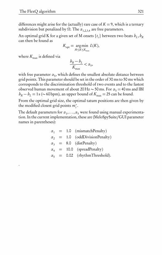
The FlexQ algorithm 321
differences might arise for the (actually) rare case of K = 9, which is a ternarysubdivision but penalized by Ω. The α1,2,3,4 are free parameters.
An optimal grid K for a given set of M onsets ti between two beats bL, bRcan then be found as
Kopt = argminM≤K≤Kmax
L(K),
where Kmax is defined viabR− bL
Kmax<α5,
with free parameter α5, which defines the smallest absolute distance betweengrid points. This parameter should be set in the order of 30 ms to 50 ms whichcorresponds to the discrimination threshold of two events and to the fastestobserved human movement of about 20 Hz∼ 50ms. For α5 = 40ms and IBIbR− bL = 1s (∼ 60bpm), an upper bound of Kmax = 25 can be found.
From the optimal grid size, the optimal tatum positions are then given bythe modified closest grid points m∗i .
The default parameters for α1, . . . ,α5 were found using manual experimenta-tion. In the current implementation, these are (MeloSpySuite/GUI parameternames in parentheses):
α1 = 1.0 (mismatchPenalty)α2 = 1.0 (oddDivisionPenalty)α3 = 8.0 (distPenalty)α4 = 10.0 (spreadPenalty)α5 = 0.02 (rhythmThreshold).
.


Brief introduction to circular statistics
Klaus Frieler
In music analysis, so-called circular variables are rather common due to thecircular nature of pitch perception, i. e., the phenomenon of octave equiva-lence, but also due to metrical structures, as used in the metrical circle map.Circular variables require specific treatment if one wants to perform statisticalanalysis, since the usual formulas do not work in this case.
This can be easily seen in the case of angles, which are also circular variables.Let us assume we have measured two angels 0° and 270°, e. g., by sightinga bird from a bird watch. What is the mean of these two values? Using thestandard formula for arithmetic means the answer would be 135°, but onewould expect in fact an angle somewhere between 270° and 360° (= 0°), tobe specific it should be 315°. One approach to solving this is to use negativeangles for angles larger than 180°. In this case the arithmetic mean of 0° and−90° is−45° which is equivalent to 315°. Unfortunately, this does not workin all cases. To illustrate this, consider four angles, 0°, 90°, 180°, and 270° =−90°, with an arithmetic mean of 45°. But intuitively, the mean is somehowundefined, because the four angles point in all four directions, for which nomean direction can be reasonably assigned. Another, related problem is thatthere is no consistent way to assign a value to 180°.
A solution to this problem lies in actually mapping the angles to points onthe unit circle in the x, y-plane. This can be done using polar coordinates,which are defined by
x = r cosφy = r sinφ,
where a vector (x, y) is represented with an angle φ= arctan y/x and mag-nitude/length r =
p
x2+ y2. Vectors on the unit circle have by definition a

324 Klaus Frieler
length of r = 1, so we map angles (measured in radians26) to the vector
z = (cosφ, sinφ).
With this embedding of angles into the x, y-plane, the standard formula cannow be used for this 2d vectors. The arithmetic mean of a vector is definedby arithmetic means of the coördinates, i. e., for vectors zi = (xi , yi )1≤i≤Nthe mean vector is given by
z =1N
N∑
i=1
zi =1N
N∑
i=1
zi (xi , yi ) =
1N
N∑
i=1
xi ,1N
N∑
i=1
yi
=: (x, y).
For the embedding of N circular variablesφi this yields the so-called resultantvector
z =
1N
N∑
i=1
cosφi ,1N
N∑
i=1
sinφi
=: R(cosφ, sinφ,
where we defined the resultant length R and the resultant angle φ, whichis possible, because the resultant vector is a normal vector in the x, y-plane,though not necessarily on the unit circle; in fact, one can show that theresultant vector lies generally inside the unit circle, i. e., R≤ 1.
The resultant angle can interpreted as the mean angle of a sample of angles,the resultant length is a measure for the variance of the sample. Indeed, thecircular variance is defined as
s2 = 1−R,
with values between 0 and 1.
The circular standard deviation is, however, defined not as the square root ofthe circular variance but via
s =
√
√
√ln1
R2 =
Æ
−2 ln R,
with values between 0 and∞27.
26In radians 360° corresponds to 2π, so every angle α in degree is 2πα/360 in radians.27This definition stems from the observation that this formula is an estimator of the standard
deviation of the circular normal distribution.

Circular statistics 325
Sometimes, the circular dispersion is also used for the analysis of variance itis defined as
δ =1−R
2
2R,
also with values between 0 and 1.
Let us consider our four angles example from above. The embedding resultsin the vectors z1 = (1,0), z2 = (0,1), z3 = (−1,0), z4 = (0,−1). The resultantvector is thus
z =14(z1+ z2+ z3+ z4) = (0,0).
Since the resultant vector is the origin in the x, y-plane, it has no reasonablydefined angle! This corresponds to our intuition that a mean direction is notwell-defined in this case. The resultant length is R= 1, hence the variance ismaximal, s2 = 1. This also correspond well to our intuition since all directionsare equally present. Accordingly, the circular standard deviation in this case isalso maximal s =∞. What is the result for our first example with embeddingz1 = (1,0), z2 = (0,−1)? The resultant vector is
z =12(z1+ z2) =
12
,−12
,
and the resultant length is R=q
12 , the resultant angle is
φ= arctan y/x = arctan(−1) =−π4≡−45°,
as desired.


Glossary
In the following glossary, several terms used throughout this book are brieflyexplained. Since readers of this book are expected to come from varyingareas of research and to have differing degrees of knowledge, these briefexplanations should be of help for quick reference. Included are several termsfrom jazz practice, jazz theory, and music theory, some statistical terms,as well as several names (and abbreviations) for musical features that areimplemented within the MeloSpy software. Some of these features are furtherdetailed in Chapter Computational melody analysis; additionally, there aremore technical definitions available within the online documentation.28
Accentemphasis on a particular tone in contrast to its neighboring tones, eitherby playing it differently (louder, special attack etc.) or by perceptualsalience (e.g., highest tone or last tone within a phrase, tones on beatsetc.) or both.
Algorithmself-contained sequence of actions, e. g., calculation or data processing,to be performed by a computer.
Arpeggioa chord broken into a sequence of tones.
Bendthe effect of bending and releasing the pitch of a tone upwards (inthe case of the guitar) or downwards (in the case of brass and reedinstruments).
28See especially http://jazzomat.hfm-weimar.de/commandline_tools/melfeature/melfeature_features.html.

328 Glossary
CDPC→Chordal Diatonic Pitch Class.
CDPCX→Extended Chordal Diatonic Pitch Class.
Chord changessuccession of musical chords.
Chordal Diatonic Pitch Class (cdpc)→diatonic pitch classes in relation to the root pitch of a given chord(based on major and dorian scales) plus additional symbols for thenon-diatonic pitches.
Chordal Pitch Class (cpc)→pitch class of a tone in relation to the root pitch of a given chordwhich has pitch class 0.
Chorusone round within the cyclical form of a jazz piece, given that withinpieces of chorus-form the→chord changes are repeated again and againduring a performance. The term originated from the final chorus parts(sung by a chorus) of American popular songs which follow the openingverse(s) sung by one singer only; in jazz those verses are omitted inmost cases and one or several improvised solos are played, lasting oneor several choruses.
Chromaticwith several pitches each a semitone above or below the other.
Chromaticitypercentage of semitone intervals in proportion to all intervals.
Constant structuresa technique to achieve coherence while improvising→outside whichmostly relies on the repetition or transposition of certain intervalstructures.
Contoura curve that tracks the absolute pitches over time.

Glossary 329
CPC→Chordal Pitch Class.
Densitya function whose values at any given point can be interpreted as pro-viding a relative likelihood of the variable (in percentage).
Diatonicwith seven pitches within an octave but with varying intervals (hepta-tonic scale), in contrast to→chromatic scales and→pentatonic scales.
Entropythe degree of predictability (or information content) within a system orstructure subject to random processes; measured normally in bits (i. e.,the mean number of yes-no-questions one has to ask to identify anyresult from such a random process). Entropy is maximal for uniformlydistributed random variables, i. e., where each event has the same prob-ability. Normalized entropy is entropy divide by the maximal possibleentropy for this process and attains values between 0 (perfect order orredundancy) and 1 (high complexity or chaos).
Extended Chordal Diatonic Pitch Class (cdpcx)variant of→Chordal Diatonic Pitch Class with additional symbols forthe non-diatonic pitches.
Fall-offeffect caused by the pitch gliding downwards at the end of a tone.
Fundamental Frequencythe lowest frequency of a periodic waveform; in music and speech oftencorrelated to the perceived pitch of a sound.
Fuzzy Duration Classclassification of durations (very short, short, long, very long) in regardto meter (relative) or time (absolute).
Fuzzy Interval Classclassification of intervals (big jump, jump, leap, step—up and down,resp.—and repetition).

330 Glossary
Guide-tone linea melodic line that guides through a chord progression. Guide-tonelines consist of different chord tones and mostly progress by intervalsteps.
Histograma graphical representation of the distribution of data by representingthe frequency or overall percentage of a certain category or class. Forcontinuous numerical data, classes have to be defined beforehand.
Intensity1) a metaphor to describe the strength, magnitude, density, vehemence,or level of music;
2) in an acoustical sense: a relative measure for the momentary degreeof dynamics; normally correlated with the degree of perceived loudness.
Inter-onset interval (IOI)time interval between the onsets of two successive tones.
Intonationthe pitch accuracy of a musical instrument or of a musician’s or singer’srealization of pitches according to a certain→tuning system.
IOI→Inter-onset interval.
Laid backplaying ‘behind the beat’, i. e., with a tendency to place tones laterthan the nominal metrical position in a given metrical frame, e. g., asprovided by the rhythm section. Cf.→Micro-rhythm.
Lick1) a colloquial term for a succession of tones that are played regularlyby a musician;
2) a category for→midlevel units with a certain rhythmic and melodicconciseness—in contrast to an uniform line–, but less singable than amelody.
MCM→Metrical circle map.

Glossary 331
Meana value for the central tendency (or average) of a metric data sample ordistribution.
Medianmeasure for the central tendency of a data sample or distribution thatseparates the higher half from the lower one, i. e., above and below themedian 50 % of the data can be found. More robust to outliers thanthe→Mean.
Metrical Circle Map (mcm)a representation of meter by dividing a bar in N equal time spans; inthis publication mostly N = 48 is used (cf. Frieler, 2007, 2008).
Micro-rhythmtiming nuances in the placement of tones; slight deviations from ideal-ized metronomic time frames or time frames provided by other players.
Midlevel annotationan annotation technique encompassing the segmentation of a melodyinto→midlevel units, the categorization of those units, and the anno-tation of references back to previous midlevel units (see Frieler et al.,2016a and Chapter Computational melody analysis for more details).
Midlevel unita musical unit on a middle level, i. e., between the level of form sectionsand that of musical cells or motives. Since a midlevel unit is conceivedto represent a musical decision or idea, it is often as long as a musical→phrase, but could also be shorter, i. e., phrases can consist of severalmidlevel units.
N-grama contiguous sequence of N items taken from a given sequence of tonesor other musical elements.
Offbeatpoints in time or tones positioned on these points that do not fall on abeat.

332 Glossary
Outsidetones or lines contrasting to or deviating from a given harmony, chord,or mode.
Parsons codea simple notation of melodic motion, basically: interval up, intervaldown and pitch repetition (proposed by Denys Parsons in his bookThe Directory of Tunes and Musical Themes, 1975).
Patterna succession of elements—e. g., tones, intervals, durations—which isrepeated or occurs several times.
Pentatonicscales with five→pitch classes.
Phrasea melodic unit or perceptional chunk of the melodic stream; phraseshave a complete musical sense of their own, or are separated before andafter by rests, or can be sung or played using a single breath.
Pitch Class (pc)a set of all pitches of the same chroma, i. e., lying a whole number ofoctaves apart; e. g., the pitch class C consists of the Cs in all octaves.
Pitch Wavinesspercentage of tones within a melody that are preceded and followedby changes of intervallic direction, i. e., local maxima and minima of apitch contour.
Postbopa rather vague umbrella term for a style of jazz emerging in the 1960sthat developed from hardbop and bebop and contrasts to avant-gardejazz and fusion music.
Scatter plota graphical representation that is used to display the paired values fortwo variables for a set of data units.
Self-similarity matrixa graphical representation of similar sequences in a data series.

Glossary 333
Side-stepping (side-slipping)technique of improvising →outside by shifting chords or lines onesemitone upwards or downwards.
Significancestatistical measure for the likelihood that a statistical result is not purelydue to chance. Statistical significance is computed by one of varioussignificance tests and is expressed as the probability (‘p value’) that theresult could have been generated by chance; by convention, if that prob-ability is lower than 5 % ( p < .05), the result is termed “significant”, ifit is lower than 1 % ( p < .01), “highly significant”.
Slideeffect caused by the pitch gliding up at the beginning of a tone.
Source separationprocedures in digital signal processing with the objective of recover-ing the original component signals of a certain sound source from acombined or complex signal.
Standard deviationa measure for the amount of variation or dispersion of a set of datavalues in regard to their→mean.
Swing ratioratio of the longer to the shorter eighth in a line played with swingfeeling.
Syncopationin general, the temporary displacement of an accent from a strongto a weak metrical position; in a narrower sense (as often used inthis publication), the shifting of a tone from a beat to an →offbeatposition immediately before the beat, while leaving the beat empty(‘anticipation’).
Syncopicitymeasure for the degree of→syncopation within a given musical unit;percentage of syncopated tones.
Timbreperceived sound quality of a sound or tone, often in relation to the
334 Glossary
composition of its harmonics and noise over time; quality that differsbetween two different tones of equal loudness and pitch.
Tonal Diatonic Pitch Class (tdpc)→pitch class in relation to the overall tonal center of a piece and to its→diatonic scale; only pitch classes of the diatonic scale of the tonalityare considered.
Tonal Pitch Class (tpc)→pitch class in relation to the overall tonal center of a piece of music.
Tuning (system)the practice of adjusting musical instruments or devices according to aspecific system of pitches, often in relation to a fixed reference pitch.The most common tuning in contemporary Western Music is 12-toneequal temperament (12-TET), i. e., an octave is divided in twelve equalintervals, with a reference pitch A4 of 440 Hz.
Variancea measure for the amount of variation or dispersion within a set of datavalues; the square of the→standard deviation.
Vectora geometrical object that has a magnitude (or length) and a directionin several (N ) dimensions. Often used in a more abstract sense for aordered collection of N values.
Vibratoa more or less regular modulation of a tone; pulsating change of itspitch and/or dynamics.
Walking bassa style of bass accompaniment with a regular quarter note movementsimilar to the regular alternation of feet while walking. Walking bass ac-companiment was developed during the swing era and is very commonamong various modern jazz styles.

References
Abeßer, J., Balke, S., Frieler, K., Pfleiderer, M., & Müller, M. (2017). Deeplearning for jazz walking bass transcription. In Proceedings of theAES International Conference on Semantic Audio. Erlangen, Germany.Retrieved from https://www.audiolabs-erlangen.de/resources/MIR/2017-AES-WalkingBassTranscription/
Abeßer, J., Cano, E., Frieler, K., & Pfleiderer, M. (2014). Dynamics in jazzimprovisation – score-informed estimation and contextual analysis oftone intensities in trumpet and saxophone solos. In Proceedings ofthe 9th Conference on Interdisciplinary Musicology (CIM) (pp. 156–161).Berlin, Germany.
Abeßer, J., Cano, E., Frieler, K., Pfleiderer, M., & Zaddach, W.-G. (2015).Score-informed analysis of intonation and pitch modulation in jazz so-los. In Proceedings of the 16th International Society for Music InformationRetrieval Conference (ISMIR). Málaga, Spain.
Abeßer, J., Frieler, K., Cano, E., Pfleiderer, M., & Zaddach, W.-G. (2017).Score-informed analysis of tuning, intonation, pitch modulation, anddynamics in jazz solos. IEEE/ACM Transactions on Audio, Speech, andLanguage Processing, 25(1), 168–177.
Abeßer, J., Pfleiderer, M., Frieler, K., & Zaddach, W.-G. (2014). Score-informed tracking and contextual analysis of fundamental frequencycontours in trumpet and saxophone jazz solos. In Proceedings of the 17thInternational Conference on Digital Audio Effects (DAFx–14). Erlangen,Germany.
Abeßer, J., & Schuller, G. (2017). Instrument-centered music transcription ofsolo bass guitar recordings. IEEE/ACM Transactions on Audio, Speech,and Language Processing, 25(9), 1741–1750.
Arzt, A. (2016). Flexible and robust music tracking. Universität Linz.Atkins, E. T. (Ed.). (2003). Jazz planet. Jackson: University Press of Missis-
sippi.Baker, D. (1985). How to play bebop (Vol. 1). Bloomington: Frangipani Press.

336 References
Balke, S., Dittmar, C., Abeßer, J., Frieler, K., Pfleiderer, M., & Müller, M.(2017). Bridging the gap. Enriching YouTube videos with jazz musicannotations. Frontiers in Digital Humanities (accepted).
Ballou, G. (2008). Handbook for sound engineers (4th ed.). Taylor & Francis.Barnhart, S. (2005). The world of jazz trumpet. A comprehensive history &
practical philosophy. Milwaukee, WI: Hal Leonard.Barrett, S. (2006). Kind of Blue and the economy of modal jazz. Popular
Music, 25(2), 185–200.Berliner, P. F. (1994). Thinking in jazz. The infinite art of improvisation.
Chicago: University of Chicago Press.Bickl, G. (2000). Chorus und Linie. Zur harmonischen Flexibilität in der
Bebop-Improvisation (= Jazzforschung / Jazz Research, Vol. 32). Graz:Akademische Druck- und Verlagsanstalt.
Bjerstedt, S. (2014). Storytelling in jazz improvisation. Implications of a richintermedial metaphor. Lund: Lund University Publications.
Bohlman, P. V., & Plastino, G. (2016). Jazz worlds, world jazz. Chicago:University of Chicago Press.
Bowen, J. A. (2011). Recordings as sources in jazz. A performance historyof “Body and Soul”. In Five Perspectives on “Body and Soul” and OtherContributions to Music Performance Research. Proceedings of the “Interna-tional Conference on Music Performance Analysis” (pp. 15–27). Zürich:Chronos.
Bregman, A. S. (1990). Auditory scene analysis. The perceptual organization ofsound (2nd ed.). Cambridge: MIT-Press.
Breiman, L. (2001). Random forests. Machine Learning, 45(1), 5–32.Brogan, D. (1985, September). Branford Marsalis feels the zing
and the sting of instant pop. Chicago Tribune. Retrievedfrom http://articles.chicagotribune.com/1985-09-05/features/8502280144_1_branford-marsalis-wynton-marsalis-live-aid
Bronson, B. H. (1949). Mechanical help in the study of folk song. Journal ofAmerican Folklore, 62, 81–90.
Brownell, J. (1994). Analytical models of jazz improvisation. Jazzforschung /Jazz Research, 26, 9–29.
Cano, E., Schuller, G., & Dittmar, C. (2014). Pitch-informed solo and accom-paniment separation: towards its use in music education applications.EURASIP Journal on Advances in Signal Processing, 1–19.
Cano, P., Batlle, E., Kalker, T., & Haitsma, J. (2005). A review of audiofingerprinting. The Journal of VLSI Signal Processing, 41(3), 271–284.
Chilton, J., & Kernfeld, B. (2002). Hinton, Milt. In The New Grove Dictionaryof Jazz (2nd ed., Vol. 2, pp. 245–246). New York: Grove.

References 337
Cohen, J. (1988). Statistical power analysis for the behavioral sciences (2nd ed.).New York: Lawrence Erlbaum Associates.
Cole, G. (2006). The last Miles. The music of Miles Davis, 1980–1991 (repr. inpaperback ed.). London: Equinox.
Coleman, S. (n.d.-a). Biography. Retrieved 2017-08-15, from http://m-base.com/biography/
Coleman, S. (n.d.-b). Symmetrical Movement Concept. Retrieved 2017-08-15,from http://m-base.com/essays/symmetrical-movement-concept/
Cook, N. (2004). Computational and comparative musicology. In E. Clarke& N. Cook (Eds.), Empirical musicology. Aims, methods, prospects, (pp.103–126). Oxford: Oxford University Press.
Cuthbert, M. S., & Ariza, C. (2010). music21. A toolkit for computer-aidedmusicology and symbolic music data. In Proceedings of the InternationalSymposium on Music Information Retrieval 11 (pp. 637–642).
D’Agostino, R. B. (1971, August). An omnibus test of normality for moderateand large size samples. Biometrika, 58(2), 341–348.
DeClercq, T., & Temperley, D. (2011). A corpus analysis of rock harmony.Popular Music, 30, 47–70.
DeVeaux, S. (1991). Constructing the jazz tradition. Jazz historiography.Black American Literature Forum, 25, 525–560.
DeVeaux, S. (1997). The birth of bebop. A social and musical history. Berkeley:University of California Press.
DeVeaux, S., & Giddins, G. (2009). Jazz. New York: Norton.Dittmar, C., Pfleiderer, M., Balke, S., & Müller, M. (2017). A swingogram rep-
resentation for tracking micro-rhythmic variation in jazz performances.Journal of New Music Research, 46.
Dittmar, C., Pfleiderer, M., & Müller, M. (2015). Automated estimation ofride cymbal swing ratio in jazz recordings. In M. Müller & F. Wiering(Eds.), Proceedings of the 16th ISMIR Conference, Málaga, Spain, October26–30, 2015 (pp. 271–277).
Dowling, W. J., & Fujitani, D. (1971). Contour, interval, and pitch recogni-tion in memory for melodies. The Journal of the Acoustical Society ofAmerica, 49(2, Suppl. 2), 524–531.
Eerola, T., & Toiviainen, P. (2004). MIDI toolbox: MATLAB tools for musicresearch. University of Jyväskylä.
Finkelman, J. (1997). Charlie Christian and the role of formulas in jazzimprovisation. Jazzforschung / Jazz Research, 29, 159–188.
Fletcher, N. H., & Rossing, T. D. (1998). The physics of musical instruments(2nd ed.). New York: Springer.
Forte, A. (1973). The structure of atonal music. New Haven: Yale UniversityPress.

338 References
Fraisse, P. (1982). Rhythm and tempo. In D. Deutsch (Ed.), The psychology ofmusic (pp. 149–180). New York: Academic Press.
Friberg, A., & Sundström, A. (2002). Swing ratios and ensemble timing injazz performance. evidence for a common rhythmic pattern. MusicPerception, 19, 333–349.
Frieler, K. (2007). Visualizing music on the metrical circle. In Proceedings ofthe 8th International Symposium on Music Information Retrieval, ISMIR2007. Wien: OCG.
Frieler, K. (2008). Metrical circle map and metrical Markov Chains. InA. Schneider (Ed.), Systematic and comparative musicology. Frank-furt/M., Bern: P. Lang.
Frieler, K. (2009). Mathematik und kognitive Melodieforschung. Grundlagenfür quantitative Modelle. Hamburg: Dr. Kovac.
Frieler, K., & Lothwesen, K. (2012). Gestaltungsmuster und Ideenfluss inJazzpiano-Improvisationen. Eine Pilotstudie zum Einfluss von Tempo,Tonalität und Expertise. In A. C. Lehmann, A. Jeßulat, & C. Wünsch(Eds.), Kreativität – Struktur und Emotion (pp. 256–265). Würzburg:Königshausen & Neumann.
Frieler, K., & Pfleiderer, M. (2017). Onbeat oder offbeat? Überlegungenzur symbolischen Darstellung von Musik am Beispiel der metrischenQuantisierung. In M. Eibl & M. Gaedke (Eds.), INFORMATIK 2017(pp. 111–125). Bonn: Gesellschaft für Informatik.
Frieler, K., Pfleiderer, M., Abeßer, J., & Zaddach, W.-G. (2016a). Midlevelanalysis of monophonic jazz solos. A new approach to the study ofimprovisation. Musicae Scientiae, 20(2), 143–162.
Frieler, K., Pfleiderer, M., Abeßer, J., & Zaddach, W.-G. (2016b). “Tellinga story”. On the dramaturgy of monophonic jazz solos. EmpiricalMusicology Review, 11(1). Retrieved from http://emusicology.org/article/view/4959
Gabbard, K. (Ed.). (1995a). Jazz among the discourses. Durham: DukeUniversity Press.
Gabbard, K. (Ed.). (1995b). Representing jazz. Durham: Duke UniversityPress.
Gabbard, K. (1996). Jammin’ at the margins. Jazz and the American cinema.Chicago: University of Chicago Press.
Gans, C. J. (2017). Saxophonist completes final pilgrimage. Retrievedfrom http://www.michaelbreckerliverecordings.com/Reviews/Pilgrimage%20review%20by%20Charles%20Gans%20Associared%20Press.pdf
Gioia, T. (1992). West Coast jazz: modern jazz in California, 1945–1960. NewYork: Oxford University Press.

References 339
Givan, B. (2016). Rethinking interaction in jazz improvisation. Music TheoryOnline, 22(3).
Gliesche, G. (2006). Paul Desmond. Der Poet auf dem Altsaxophon. Heidenau:PD-Verl.
Goldsher, A. (2002). Hard bop academy: the sidemen of Art Blakey and theJazz Messengers (1st ed.). Milwaukee: Hal Leonard.
Goodrick, M. (1987). The advancing guitarist. Applying guitar concepts &techniques. Milkwaukee: Hal Leonard.
Goodwin, J. D. (2015, January). Branford Marsalis, taking the long view.Boston Globe. Retrieved from https://www.bostonglobe.com/arts/music/2015/01/24/branford-marsalis-taking-long-view/v61yiNOgm1dbZuQCfWDsDK/story.html
Gordon, R. (1986). Jazz West Coast. The Los Angeles jazz scene of the 1950s.London, New York: Quartet Books.
Grella, G. (2015). Bitches brew. New York: Bloomsbury Academic.Gridley, M. C. (1978). Jazz styles. History and analysis. Englewood Cliffs:
Prentice Hall.Harrison, M., & Kernfeld, B. (2001). Desmond, Paul. In B. Kernfeld (Ed.),
The New Grove Dictionary of Jazz (2nd ed., Vol. 1, pp. 605–606). NewYork: Grove.
Harte, Christopher, Sandler, M., Samer, A., & Gómez, E. (2005). Sym-bolic representation of musical chords. A proposed syntax for textannotations. In Proceedings of the 6th International Conference on Mu-sic Information Retrieval (ISMIR) (pp. 66–71). Queen Mary, London.Retrieved from http://ismir2005.ismir.net/proceedings/1080.pdf
Hellhund, H. (1985). Cool Jazz. Grundzüge seiner Entstehung und Entwicklung.Mainz: Schott.
Hodeir, A. (1956). Hommes et problèmes du jazz. Suivi de la religion du jazz.Paris: Portulan.
Hodson, R. (2007). Interaction, improvisation, and interplay in jazz. NewYork/London: Routledge.
Huron, D. (1996). The melodic arch in western folksongs. Computing inMusicology, 10, 3–23.
Huron, D. (1999). The Humdrum toolkit. Software for music research. Re-trieved 2016-01-02, from http://dactyl.som.ohio-state.edu/Humdrum(Published Online Manual)
ISO16:1975. (1975). Acoustics – Standard tuning frequency (standard mu-sical pitch) (Standard Specification). International Organization forStandardization.
Jackson, T. A. (2012). Blowin’ the blues away. Performance and meaning onthe New York jazz scene. Berkeley: University of California Press.

340 References
Jost, E. (1975). Free Jazz. Stilkritische Untersuchungen zum Jazz der 60er Jahre.Mainz: Schott.
Jost, E. (1987). Europas Jazz 1960–80. Frankfurt: Fischer.Jost, E. (2003). Sozialgeschichte des Jazz (1st ed.). Frankfurt: Zweitausendeins.Kelman, J. (2007, September). Chris Potter Underground: Follow
the Red Line: Live at the Village Vanguard. Retrieved fromhttps://www.allaboutjazz.com/follow-the-red-line-live-at-the-village-vanguard-chris-potter-sunnyside-records-review-by-john-kelman.php
Kernfeld, B. (1995). What to listen for in jazz. New Haven and London: YaleUniversity Press.
Kernfeld, B. (2002a). Hubbard, Freddie. In The New Grove Dictionary ofJazz (2nd ed., Vol. 2, pp. 288–289). New York: Grove.
Kernfeld, B. (2002b). Improvisation. In B. Kernfeld (Ed.), The New GroveDictionary of Jazz (2nd ed., Vol. 2, pp. 313–322). New York: Grove.
Kernfeld, B. (2002c). Shaw, Woody. In The New Grove Dictionary of Jazz(2nd ed., Vol. 3, pp. 557–558). New York: Grove.
Kerschbaumer, F. (1971). Zum Personalstil von Miles Davis. Jazzforschung /Jazz Research, 3/4, 225–232.
Kerschbaumer, F. (1978). Miles Davis. Stilkritische. Untersuchungen zurmusikalischen Entwicklung seines Personalstils. Graz: AkademischeDruck- und Verlags-Anstalt.
Kerschbaumer, F. (2003). Hubbard, Freddie. In Die Musik in Geschichteund Gegenwart. Personenteil (2nd ed., Vol. 9, pp. 435–437). Kassel:Bärenreiter.
Kerschbaumer, F. (2006). Shaw, Woody Herman II. In Die Musik in Geschichteund Gegenwart. Personenteil (2nd ed., Vol. 15, pp. 685–686). Kassel:Bärenreiter.
Kipperman, J. P. (2016). Milt ‘The Judge’ Hinton. A musical analysis (Unpub-lished doctoral dissertation). University of Miami.
Kissenbeck, A. (2007). Jazztheorie. Kassel: Bärenreiter.Knees, P., & Schedl, M. (2016). Music similarity and retrieval. Heidelberg:
Springer.Krieger, F. (1995). Jazz-Solopiano. Zum Stilwandel am Beispiel ausgewählter
"‘Body and Soul"’-Aufnahmen von 1938-–1992 (= Jazzforschung/JazzResearch, Vol. 27). Graz: Akademische Druck- und Verlagsanstalt.
Kunzler, M. (2002). Desmond, Paul. In M. Kunzler (Ed.), Jazz-Lexikon (2nded., pp. 292–293). Reinbek bei Hamburg: Rohwolt.
Kunzler, M. (2004a). Hubbard, Frederick Dewyne (“Freddie”). In Jazz-Lexikon (2nd ed., Vol. 2, pp. 581–583). Reinbek bei Hamburg: Ro-hwolt.

References 341
Kunzler, M. (2004b). Shaw, Woody Herman II. In Jazz-Lexikon (2nd ed.,Vol. 2, pp. 1205–1206). Reinbek bei Hamburg: Rohwolt.
Langner, J., & Goebel, W. (2003). Visualizing expressive performance intempo–loudness space. Computer Music Journal, 27(4), 69–83.
Lee, C.-H., Shih, J.-L., Yu, K.-M., & Lin, H.-S. (2009). Automatic musicgenre classification based on modulation spectral analysis of spectraland cepstral features. IEEE Transactions on Multimedia, 11(4), 670–682.
Lee, D. D., & Seung, H. S. (2001). Algorithms for non-negative matrixfactorization. Advances in Neural Information Processing Systems, 556–562.
Lerdahl, F., & Jackendoff, R. (1983). A generative theory of tonal music.Cambridge, MA: The MIT press.
Levenshtein, V. I. (1965). Binary codes capable of correcting deletions,insertions, and reversals. Doklady Akademii Nauk SSSR, 163(4), 845–848. (English translation in: Soviet Physics Doklady, 10(8), pp. 707–710,1966)
Levine, M. (1995). Jazz theory book. Petaluma: Sher Music.Liebman, D. (2006). A chromatic approach to jazz harmony and melody.
Rottenburg: Advance Music.Lomax, A. (1976). Cantometrics. An approach to the anthropology of music.
Berkeley: University of California Extension Media Center.Mauch, M. (2010). Automatic chord transcription from audio using computa-
tional models of musical context (Unpublished doctoral dissertation).Queen Mary University of London, London.
Mauch, M., & Dixon, S. (2014). PYIN: A fundamental frequency estimatorusing probabilistic threshold distributions. In Proceedings of the 39thIEEE International Conference on Acoustics, Speech and Signal Processing(ICASSP) (pp. 659–663). Florence, Italy.
Meyers, J. P. (2015). Standards and signification between jazz and fusion:Miles Davis and “I Fall in Love Too Easily,” 1963–1970. Jazz Perspectives,9(2), 113–136.
Milkowski, B. (2012). Like it is: The Branford Marsalis interview. BillMilkowski’s extended conversation from the october issue. Retrievedfrom https://jazztimes.com/features/like-it-is-the-branford-marsalis-interview/
Milkowski, B. (2017). Chris Potter – Bio. Retrieved from http://chrispotter.net/home/biography
Monson, I. (1996). Saying something. Jazz improvisation and interaction.Chicago: University of Chicago Press.
342 References
Müllensiefen, D., & Frieler, K. (2004). Cognitive adequacy in the mea-surement of melodic similarity. Algorithmic vs. human judgments.Computing in Musicology, 13, 147–176.
Müllensiefen, D., Frieler, K., & Pfleiderer, M. (2009). The perception ofaccents in pop music melodies. Journal of New Music Research, 38(1),19–44.
Müllensiefen, D., Wiggins, G., & Lewis, D. (2008). High-level featuredescriptors and corpus-based musicology. Techniques for modellingmusic cognition. In A. Schneider (Ed.), Systematic and ComparativeMusicology (= Hamburger Jahrbuch für Musikwissenschaft, Vol. 25) (pp.133–156). Frankfurt/M., Bern: P. Lang.
Müller, C. (2017). Doing Jazz. Zur Konstitution einer kulturellen Praxis.Weilerstwist: Velbrück.
Müller, M. (2015). Fundamentals of music processing: Audio, analysis, algo-rithms, applications. Heidelberg: Springer.
Müller, M., & Ewert, S. (2011). Chroma Toolbox: MATLAB implementa-tions for extracting variants of chroma-based audio features. In Proceed-ings of the 12th International Society for Music Information RetrievalConference (ISMIR) (pp. 215–220). Miami, USA.
Nicholson, S. (2005). Is jazz dead? (Or has it moved to a new address). NewYork: Routledge.
Nicholson, S. (2014). Jazz and culture in a global age. Boston: Northeastern.Norgaard, M. (2008). Descriptions of improvisational thinking by artist-level
jazz musicians (Unpublished doctoral dissertation). University of Texas,Austin.
Norgaard, M. (2014). How jazz musicians improvise. The central role ofauditory and motor patterns. Music Perception: An InterdisciplinaryJournal, 31(3), 271–287.
O’Meally, R. G. (Ed.). (2007). The jazz cadence of American culture. NewYork: Columbia University Press.
O’Meally, R. G., Edwards, B. H., & Griffin, F. J. (Eds.). (2004). Uptownconversations. The new jazz studies. New York: Columbia UniversityPress.
Owens, T. (1974). Charlie Parker. Techniques of improvisation (Unpublisheddoctoral dissertation). University of California, Los Angeles.
Owens, T. (1995). Bebop. The music and its players. New York: OxfordUniversity Press.
Owens, T. (2002). Analysing jazz. In M. Cooke & D. Horn (Eds.), TheCambridge companion to jazz (pp. 286–297). New York: CambridgeUniversity Press.

References 343
Painter, T., & Spanias, A. (2000). Perceptual coding of digital audio. Proceed-ings of the IEEE, 88(4), 451–515.
Panken, T. (2016). For Harry Connick’s 49th birthday, a jazziz feature articlefrom 2002. Retrieved from https://tedpanken.wordpress.com/2016/09/11/for-harry-connicks-49th-birthday-a-jazziz-feature-article-from-2002/
Parsons, D. (1975). The directory of tunes and musical themes. London: BritishLibrary.
Peeters, G. (2004). A large set of audio features for sound description (similarityand classification) in the CUIDADO project. IRCAM.
Pfleiderer, M. (2005). Steve Coleman. In P. N. Wilson (Ed.), Jazz Klassiker(pp. 801–807). Stuttgart: Reclam.
Pfleiderer, M. (2006). Rhythmus. Psychologische, theoretische und stilanalytischeAspekte populärer Musik. Bielefeld: transcript.
Pfleiderer, M. (2011). “Body and Soul” and the mastery of the jazz tenor saxo-phone. In Five perspectives on “Body and Soul” and other contributions tomusic performance research. Proceedings of the “International Conferenceon Music Performance Analysis” (pp. 29–43). Zürich: Chronos.
Pfleiderer, M., Frieler, K., & Zaddach, W.-G. (2016). Pitch class hierarchiesin Miles Davis’s “So What”. Reconsidering modal jazz improvisationwith computer-based analysis tools. In W. Auhagen & W. Hirschmann(Eds.), Beitragsarchiv zur Jahrestagung der Gesellschaft für MusikforschungHalle/Saale 2015 – Musikwissenschaft: die Teildisziplinen im Dialog.Mainz: Schott-Campus.
Polkow, D. (1989, August). Jazz vs. Pop. For Branford Marsalis,it doesn’t pay to be a purist. Chicago Tribune. Retrievedfrom http://articles.chicagotribune.com/1989-08-07/features/8901030105_1_branford-marsalis-kenny-kirkland-wynton
Porter, L. (1985). Lester Young. Boston: Twayne.Porter, L. (1998). John Coltrane, his life and music. Ann Arbor: University of
Michigan Press.Porter, L., Ullman, M., & Hazell, E. (Eds.). (1993). Jazz. From its origins to
its present. Englewood Cliffs: Prentice Hall.Poutiainen, A. (1999). Brecker and patterns. An analysis of Michael Brecker’s
melodic and instrumental devices. (Unpublished doctoral dissertation).Sibelius Academy Helsinki, Helsinki.
Prouty, K. E. (2010). Toward jazz’s “official” history. The debates anddiscourses of jazz history textbooks. Journal of Music History Pedagogy,1(2), 19–43.

344 References
Putschögl, G. (1993). John Coltrane und die afroamerikanische Oraltradition(= Jazzforschung / Jazz Research, Vol. 25). Graz: Akademische Druck-und Verlags-Anstalt.
R Development Core Team. (2008). R: A language and environment forstatistical computing. Vienna.
Ramsey, D., Brubeck, D., Brubeck, I., & Caulfield, P. (2005). Take five. Thepublic and private lives of Paul Desmond. Seattle: Parkside Publications.
Rawlings, D. F. (2003). Brecker’s blues. Transcription and theoretical analysisof six selected improvised blues solos by jazz saxophonist Michael Brecker(Unpublished doctoral dissertation). Ohio State University.
Raz, G. (2012). Branford Marsalis on sensitive musicians and the first family ofjazz. Retrieved from http://www.npr.org/sections/ablogsupreme/2012/08/11/158525752/branford-marsalis-on-sensitive-musicians-and-the-first-family-of-jazz
Reid, G. (2010, June). Branford Marsalis interviewed (1988). Family matters.Retrieved from https://www.elsewhere.co.nz/jazz/3196/branford-marsalis-interviewed-1988-family-matters/
Richardson, E. R. (2006). Structural elegance and harmonic disparity inselected solos by jazz trumpeters Freddie Hubbard and Woody Shaw.Retrieved from http://digitalcommons.lsu.edu/cgi/viewcontent.cgi?article=1028&context=gradschool_majorpapers
Rusch, R., Salley, K., & Stover, C. (2016). Capturing the ineffable. Threetranscriptions of a jazz solo by Sonny Rollins. Music Theory Online,22(3). Retrieved from http://mtosmt.org/issues/mto.16.22.3/mto.16.22.3.rusch.html
Sagee, A. (2003). Miles Davis’s improvised solos in recordings of “Walkin’”:1954–67. Annual Review of Jazz Studies, 13, 27–47.
Sandke, R. (2000). The trumpet in jazz. In B. Kirchner (Ed.), The Oxfordcompanion to jazz. Oxford, New York: Oxford University Press.
Schuller, G. (1958). Sonny Rollins and the challenge of thematic improvisa-tion. Jazz Review, November 58, 6–11.
Schuller, G. (1968). Early jazz. Its roots and musical development. Oxford,New York: Oxford University Press.
Schuller, G. (1989). The swing era. The development of jazz 1930–45. Oxford,New York: Oxford University Press.
Schütz, M. (2015). Improvisation im Jazz. Eine empirische Untersuchung beiJazzpianisten auf der Basis der Ideenflussanalyse. Hamburg: Dr. Kovac.
Seeger, C. (1958). Prescriptive and descriptive music writing. The MusicalQuaterly, 44(2), 184–195.
Selfridge-Field, E. (Ed.). (1997). Beyond MIDI. The handbook of musical codes.Cambridge: The MIT Press.
References 345
Shannon, C. E. (1948). A mathematical theory of communication. BellSystem Technical Journal, 27(3), 379–423 and 623–656.
Shipton, A. (2007). A new history of jazz (Rev. and updated ed.). New York:Continuum.
Smith, G. E. (1991). In quest of a new perspective on improvised jazz: Aview from the Balkans. The World of Music, 33(3), 29–52.
Sudnow, D. (1999). Ways of the hand. The organization of improvised conduct.Cambridge, MA: MIT Press.
Sugg, A. (2014). The influence of John Coltrane’s music on improvising saxo-phonists. Comparing selected improvisations of Coltrane, Jerry Bergonzi,and David Liebman. Lewiston: The Edwin Mellen Press.
Sullivan, L. T. (n.d.). Don Byas. Legendary jazz saxophonist. Retrieved fromhttp://donbyas.jazzgiants.net
Svorinich, V. (2015). Listen to this: Miles Davis and Bitches Brew. Jackson:University Press of Mississippi.
Temperley, D., & DeClercq, T. (2013). Statistical analysis of harmony andmelody in rock music. Journal of New Music Research, 42, 187–204.
Tercinet, A. (1986). West Coast jazz. Marseille: Parenthèses.Terefenko, D. (2014). Jazz theory. From basic to advanced study. New York:
Routledge.Tingen, P. (2001). Miles beyond. The electric explorations of Miles Davis,
1967–1991. New York: Billboard Books.Tirro, F. (1974). Constructive elements in jazz improvisation. Journal of the
American Musicological Society, 27, 285–305.Tirro, F. (1977). Jazz. A history. New York: W.W. Norton.Tjao, S. K., & Liu, K. J. R. (2010). Musical instrument recognition using
biologically inspired filtering of temporal dictionary atoms. In Proceed-ings of the 11th International Society for Music Information RetrievalConference (ISMIR) (pp. 435–440).
Tomlinson, G. (1991). Cultural dialogics and jazz. A white historian signifies.Black Music Research Jounal, 11(2), 229–264.
Valk, J. d. (1991). Chet Baker. Schaftlach: Oreos.Waters, K. (2011). The studio recordings of the Miles Davis Quintet, 1965–68.
New York: Oxford University Press.Weiskopf, W., & Ricker, R. (1993). The augmented scale in jazz. New Albany:
Jamey Aebersold Jazz.Williams, M. (1973). The Smithsonian collection of classic jazz. Smithsonian
Collection – P6 11891.Wilson, P. N. (2001). Miles Davis. Sein Leben, seine Musik, seine Schallplatten.
Waakirchen: Oreos.

346 References
Winkler, P. (1997). Writing ghost notes. The poetics and politics of transcrip-tion. In D. Schwarz, A. Kassabian, & L. Siegel (Eds.), Keeping score.Music, disciplinarity, culture (pp. 169–203). Charlottsville: UniversityPress of Virginia.
Yanow, S. (2017). Branford Marsalis, Trio Jeepy. Retrieved from http://www.allmusic.com/album/trio-jeepy-mw0000200678
Zanette, D. H. (2006). Zipf’s law and the creation of musical context. MusicaeScientiae, 10, 3–18.