Martin Markl- A Resolution (Minimal Model) of the PROP for Bialgebras
31
a r X i v : m a t h / 0 2 0 9 0 0 7 v 6 [ m a t h . A T ] 6 J a n 2 0 0 5 A RESOLUTION (MINIMAL MODEL) OF THE PROP FOR BIALGEBRAS MARTIN MARKL Abstract. This paper is concerned with a minimal resolution of the prop for bialgebras (Hopf algebras without unit, counit and antipode). We prove a theorem about the form of this resolution (Theorem 15) and give, in Section 5, a lot of explicit formulas for the differential. 1. Introduction and main results A bialgebra is a vector space V with a multiplication µ : V ⊗V → V and a comultiplication (also called a diagonal ) ∆ : V → V ⊗ V . The multiplication is associative: (1) µ(µ ⊗ 11 V ) = µ(11 V ⊗ µ), wher e 11 V : V → V denotes the identity map, the comultiplication is coassociative: (2) (11 V ⊗ ∆)∆ = (∆ ⊗ 11 V )∆ and the usual compatibility relation between µ and ∆ is assumed: (3) ∆ ◦ µ = (µ ⊗ µ)T σ(2,2) (∆ ⊗ ∆), where T σ(2,2) : V ⊗4 → V ⊗4 is defined by T σ(2,2) (v 1 ⊗ v 2 ⊗ v 3 ⊗ v 4 ) := v 1 ⊗ v 3 ⊗ v 2 ⊗ v 4 , for v 1 , v 2 , v 3 ,v 4 ∈ V (the meaning of the notation σ(2, 2) will be explained in Definition 17). We suppose that V , as well as all other algebraic objects in this paper, are defined over a field k of characteristic zero. Let B be the k-linear prop (see [9, 10] or Section 2 of this paper for the terminology) describing bialgebras. The goal of this paper is to describe a minimal model of B, that is, a differential graded (dg) k-linear prop (M, ∂ ) together with a homology isomorphism (B, 0) ρ ←− (M, ∂ ) such that (i) the prop M is free and (ii) the image of ∂ consists of decomposable elements of M (the minimality condition), Date : January 5, 2005. 2000 Mathematics Subject Classification. 16W30, 57T05, 18C10, 18G99. Key words and phrases. bialgebra, PROP, minimal model, resolution, strongly homotopy bialgebra. The author was supported by the grant GA AV ˇ CR #1019203. Preliminary results were announced at Workshop on Topology, Operads & Quantization, Warwick, UK, 11.12. 2001. 1
Transcript of Martin Markl- A Resolution (Minimal Model) of the PROP for Bialgebras
8/3/2019 Martin Markl- A Resolution (Minimal Model) of the PROP for Bialgebras
http://slidepdf.com/reader/full/martin-markl-a-resolution-minimal-model-of-the-prop-for-bialgebras 1/31
a r X i v : m a t h / 0 2 0 9 0 0 7 v 6
[ m a t h . A
T ] 6 J a n 2 0 0 5
A RESOLUTION (MINIMAL MODEL) OF THE PROP FORBIALGEBRAS
MARTIN MARKL
Abstract. This paper is concerned with a minimal resolution of the prop for bialgebras(Hopf algebras without unit, counit and antipode). We prove a theorem about the formof this resolution (Theorem 15) and give, in Section 5, a lot of explicit formulas for thedifferential.
1. Introduction and main results
A bialgebra is a vector space V with a multiplication µ : V ⊗V → V and a comultiplication
(also called a diagonal ) ∆ : V → V ⊗ V . The multiplication is associative:
(1) µ(µ ⊗ 11V ) = µ(11V ⊗ µ),
where 11V : V → V denotes the identity map, the comultiplication is coassociative:
(2) (11V ⊗ ∆)∆ = (∆ ⊗ 11V )∆
and the usual compatibility relation between µ and ∆ is assumed:
(3) ∆ ◦ µ = (µ ⊗ µ)T σ(2,2)(∆ ⊗ ∆),
where T σ(2,2) : V ⊗4 → V ⊗4 is defined by
T σ(2,2)(v1 ⊗ v2 ⊗ v3 ⊗ v4) := v1 ⊗ v3 ⊗ v2 ⊗ v4,
for v1, v2, v3, v4 ∈ V (the meaning of the notation σ(2, 2) will be explained in Definition 17).
We suppose that V , as well as all other algebraic objects in this paper, are defined over a
field k of characteristic zero.
Let B be the k-linear prop (see [9, 10] or Section 2 of this paper for the terminology)
describing bialgebras. The goal of this paper is to describe a minimal model of B, that is, a
differential graded (dg) k-linear prop (M, ∂ ) together with a homology isomorphism
(B, 0)ρ
←− (M, ∂ )
such that
(i) the prop M is free and
(ii) the image of ∂ consists of decomposable elements of M (the minimality condition),
Date: January 5, 2005.2000 Mathematics Subject Classification. 16W30, 57T05, 18C10, 18G99.Key words and phrases. bialgebra, PROP, minimal model, resolution, strongly homotopy bialgebra.The author was supported by the grant GA AV CR #1019203. Preliminary results were announced at
Workshop on Topology, Operads & Quantization, Warwick, UK, 11.12. 2001.1

8/3/2019 Martin Markl- A Resolution (Minimal Model) of the PROP for Bialgebras
http://slidepdf.com/reader/full/martin-markl-a-resolution-minimal-model-of-the-prop-for-bialgebras 2/31
2 M. MARKL
see again Section 2 where free props and decomposable elements are recalled.
The initial stages of this minimal model were constructed in [ 9, page 145] and [10,
pages 215–216]. According to our general philosophy, it should contain all information aboutthe deformation theory of bialgebras. In particular, the Gerstenhaber-Schack cohomology
which is known to control deformations of bialgebras [3] can be read off from this model as
follows.
Let E nd V denote the endomorphism prop of V and let a bialgebra structure B =
(V,µ, ∆) on V be given by a homomorphism of props β : B → E nd V . The composition
β ◦ ρ : M → E nd V makes E nd V an M-module (in the sense of [10, page 203]), therefore one
may consider the vector space of derivations Der (M, E nd V ). For θ ∈ Der (M, E nd V ) define
δθ := θ ◦ ∂ . It follows from the obvious fact that ρ ◦ ∂ = 0 that δθ is again a derivation, so
δ is a well-defined endomorphism of the vector space Der (M, E nd V ) which clearly satisfiesδ2 = 0. Then
H b(B; B) ∼= H (Der (M, E nd V ), δ),
where H b(B; B) denotes the Gerstenhaber-Schack cohomology of the bialgebra B with coef-
ficients in itself.
Algebras (in the sense recalled in Section 2) over (M, ∂ ) have all rights to be called
strongly homotopy bialgebras, that is, homotopy invariant versions of bialgebras, as follows
from principles explained in the introduction of [12]. This would mean, among other things,
that, given a structure of a dg-bialgebra on a chain complex C ∗, then any chain complex D∗,
chain homotopy equivalent to C ∗, has, in a certain sense, a natural and unique structure of an algebra over our minimal model (M, ∂ ).
For a discussion of props for bialgebras from another perspective, see [16]. Constructions
of various other (non-minimal) resolutions of the prop for bialgebras, based mostly on a dg-
version of the Boardman-Vogt W -construction, will be the subject of [6]. A completely
different approach to bialgebras and resolutions of objects governing them can be found in
a series of papers by Shoikhet [20, 21, 22], and also in a recent draft by Saneblidze and
Umble [19]. A general theory of resolutions of props is, besides [15], also the subject of
Vallette’s thesis and its follow-up [24, 25].
Let us briefly sketch the strategy of the construction of our model. Consider objects
(V,µ, ∆), where µ : V ⊗ V → V is an associative multiplication as in (1), ∆ : V → V ⊗ V is
a coassociative comultiplication as in (2), but the compatibility relation (3) is replaced by
(4) ∆ ◦ µ = 0.
Definition 1. A half-bialgebra or briefly 12
bialgebra is a vector space V equipped with a
multiplication µ and a comultiplication ∆ satisfying ( 1), ( 2 ) and ( 4).
We chose this strange name because (4) is indeed, in a sense, one half of the compatibility
relation (3). For a formal variable ǫ, consider the axiom
∆ ◦ µ = ǫ · (µ ⊗ µ)T σ(2,2)(∆ ⊗ ∆).

8/3/2019 Martin Markl- A Resolution (Minimal Model) of the PROP for Bialgebras
http://slidepdf.com/reader/full/martin-markl-a-resolution-minimal-model-of-the-prop-for-bialgebras 3/31
MINIMAL MODEL OF THE PROP FOR BIALGEBRAS 3
At ǫ = 1 we get the usual compatibility relation (3) between the multiplication and the
diagonal, while ǫ = 0 gives (4). Therefore (3) can be interpreted as a perturbation of (4)
which may be informally expressed by saying that bialgebras are perturbations of 12bialgebras.Experience with homological perturbation theory [4] leads us to formulate:
Principle. The prop B for bialgebras is a perturbation of the prop 12B for 1
2bialgebras.
Therefore there exists a minimal model of the prop B that is a perturbation of a minimal
model of the prop 12B for 12bialgebras.
We therefore need to know a minimal model for 12B. In general, props are extremely
huge objects, difficult to work with, but 12
bialgebras exist over much smaller objects than
props. These smaller objects, which we call 12
props, were introduced in an e-mail message
from M. Kontsevich [5] who called them small props. The concept of 1
2
props makes the
construction of a minimal model of 12B easy. We thus proceed in two steps.
Step 1. We construct a minimal model (Γ(Ξ), ∂ 0) of the prop 12B for 1
2bialgebras. Here
Γ(Ξ) denotes the free prop on the space of generators Ξ, see Theorem 13.
Step 2. Our minimal model (M, ∂ ) of the prop B for bialgebras will be then a pertur-
bation of (Γ(Ξ), ∂ 0), that is,
(M, ∂ ) = (Γ(Ξ), ∂ 0 + ∂ pert ),
see Theorem 15.
Acknowledegment. I would like to express my gratitude to Jim Stasheff, Steve Shnider,Vladimir Hinich, Wee Liang Gan and Petr Somberg for careful reading the manuscript and
many useful suggestions. I would also like to thank the Erwin Schrodinger International
Institute for Mathematical Physics, Vienna, for the hospitality during the period when the
first draft of this paper was completed.
My particular thanks are due to M. Kontsevich whose e-mail [5] shed a new light on the
present work and stimulated a cooperation with A.A. Voronov which resulted in [15]. Also
the referee’s remarks were extremely helpful.

8/3/2019 Martin Markl- A Resolution (Minimal Model) of the PROP for Bialgebras
http://slidepdf.com/reader/full/martin-markl-a-resolution-minimal-model-of-the-prop-for-bialgebras 4/31
4 M. MARKL
2. Structure of props and 12props
Let us recall that a k-linear prop A (called a theory in [9, 10]) is a sequence of k-vectorspaces {A(m, n)}m,n≥1 with compatible left Σm- right Σn-actions and two types of equivariant
compositions, vertical:
◦ : A(m, u) ⊗ΣuA(u, n) → A(m, n), m,n,u ≥ 1,
and horizontal:
⊙ : A(m1, n1) ⊗ A(m2, n2) → A(m1 + m2, n1 + n2), m1, m2, n1, n2 ≥ 1,
together with an identity 11 ∈ A(1, 1). props should satisfy axioms which could be read off
from the example of the endomorphism prop E nd V of a vector space V , with E nd V (m, n)
the space of linear maps Hom k(V ⊗n, V ⊗m), 11 ∈ E nd V (1, 1) the identity map, horizontalcomposition given by the tensor product of linear maps, and vertical composition by the
ordinary composition of maps. One can therefore imagine elements of A(m, n) as ‘abstract’
maps with n inputs and m outputs. See [8, 10] for precise definitions.
We say that X has biarity (m, n) if X ∈ A(m, n). We will sometimes use the operadic
notation: for X ∈ A(m, k), Y ∈ A(1, l) and 1 ≤ i ≤ k, we write
(5) X ◦i Y := X ◦ (11⊗(i−1) ⊗ Y ⊗ 11⊗(k−i)) ∈ A(m, k + l − 1)
and, similarly, for U ∈ A(k, 1), V ∈ A(l, n) and 1 ≤ j ≤ l we denote
(6) U j◦ V := (11⊗( j−1) ⊗ U ⊗ 11⊗(l− j)) ◦ V ∈ A(k + l − 1, n).
In [10] we called a sequence E = {E (m, n)}m,n≥1 of left Σm-, right Σn-k-bimodules a
core, but we prefer now to call such sequences Σ-bimodules . For any such a Σ-bimodule
E , there exists the free prop Γ(E ) generated by E . It also makes sense to speak, in the
category of props, about ideals, presentations, modules, etc, see [24, Chapter 2] for details.
Recall that an algebra over a prop A is (given by) a prop morphism α : A → E nd V .
A prop A is augmented if there exist a homomorphism ǫ : A → 1 (the augmentation ) to
the trivial prop 1 := E nd k. Therefore an augmentation is the same as a structure of an
A-algebra on the one-dimensional vector space k.
Let A+ := Ker(ǫ) denote the augmentation ideal of an augmented prop A. The space
D(A) := A+◦A+ is then called the space of decomposables and the quotient Q(A) := A+/D(A)
the space of indecomposables of the augmented prop A. Observe that each free prop Γ(E )
is canonically augmented, with the augmentation defined by ǫ(E ) := 0.
Let Γ( , ) be the free prop generated by one operation of biarity (1, 2) and one
operation of biarity (2, 1). More formally, Γ( , ) := Γ(E ) with E the Σ-bimodule
k · ⊗ k[Σ2] ⊕ k[Σ2] ⊗ k · . As we explained in [9, 10], the prop B describing bialgebras
has a presentation
(7) B = Γ( , )/IB,

8/3/2019 Martin Markl- A Resolution (Minimal Model) of the PROP for Bialgebras
http://slidepdf.com/reader/full/martin-markl-a-resolution-minimal-model-of-the-prop-for-bialgebras 5/31

8/3/2019 Martin Markl- A Resolution (Minimal Model) of the PROP for Bialgebras
http://slidepdf.com/reader/full/martin-markl-a-resolution-minimal-model-of-the-prop-for-bialgebras 6/31
6 M. MARKL
of the genus and path gradings are discussed in [15, Section 5]. The following proposition
follows immediately from the results of [15].
Proposition 3. For any fixed d, the subspaces
Span {X ∈ Γ( , )(m, n); gen(X ) = d} and Span {X ∈ Γ( , )(m, n); pth(X ) = d}
are finite dimensional.
The following formula relating the path and genus gradings was also derived in [15]:
(9) pth(X ) ≤ mn(gen(X ) + 1) for X ∈ Γ( , )(m, n).
There is, of course, also the obvious grading grd(X ) given by the number of vertices of
the graph GX . Using this grading, the decomposables of a free prop can be described as
D(Γ(E )) = Span {X ∈ Γ(E ); grd(X ) ≥ 2}.
Let us recall the following important definition [5, 15].
Definition 4. A 12
prop is a collection s = {s(m, n)} of dg (Σm, Σn)-bimodules s(m, n)
defined for all couples of natural numbers except (m, n) = (1, 1), together with compositions
(10) ◦i : s(m1, n1) ⊗ s(1, l) → s(m1, n1 + l − 1), 1 ≤ i ≤ n1,
and
(11) j◦ : s(k, 1) ⊗ s(m2, n2) → s(m2 + k − 1, n2), 1 ≤ j ≤ m2,
that satisfy the axioms satisfied by operations ◦i and j ◦, see ( 5 ), ( 6 ), in a general prop.
Remark 5. Observe that 12props as introduced above cannot have a unit 1 ∈ s(1, 1). We
choose this convention from the following reasons. There exist an obvious unital version
of 12
props, but for all examples of interest, including 12
bialgebras, the corresponding unital12
prop would satisfy s(1, 1) ∼= k. Since there clearly exists a canonical one-to-one correspon-
dence between unital 12
props enjoying this property and non-unital 12
props in the sense of
the above definition, the unit would carry no information.
Moreover, working without units enables one to define the ‘obvious grading’ grd(−) of
free 12props in a very natural way, without using graphs. The same reason lead us in [11]
to introduce pseudo-operads as non-unital versions of operads. The above considerations do
not apply to props because P(1, 1) is typically an infinite-dimensional space.
Let us denote by Γ12
( , ) the free 12
prop generated by operations and . The
following proposition, which follows again from [15], gives a characterization of the subspaces
Γ12
( , )(m, n) ⊂ Γ( , )(m, n)
in terms of the genus and path gradings introduced above.

8/3/2019 Martin Markl- A Resolution (Minimal Model) of the PROP for Bialgebras
http://slidepdf.com/reader/full/martin-markl-a-resolution-minimal-model-of-the-prop-for-bialgebras 7/31

8/3/2019 Martin Markl- A Resolution (Minimal Model) of the PROP for Bialgebras
http://slidepdf.com/reader/full/martin-markl-a-resolution-minimal-model-of-the-prop-for-bialgebras 8/31

8/3/2019 Martin Markl- A Resolution (Minimal Model) of the PROP for Bialgebras
http://slidepdf.com/reader/full/martin-markl-a-resolution-minimal-model-of-the-prop-for-bialgebras 9/31
8/3/2019 Martin Markl- A Resolution (Minimal Model) of the PROP for Bialgebras
http://slidepdf.com/reader/full/martin-markl-a-resolution-minimal-model-of-the-prop-for-bialgebras 10/31
10 M. MARKL
Remark 14. For a 12prop s, let P (s) be the augmented prop whose augmentation ideal
equals s, whose compositions ◦i and j ◦ of (5) and (6) are those of s, and other compositions
(that is, those not allowed for 12props) are set to be zero. Theorem 13 expresses the factthat the prop P (12b
!) is the quadratic dual of the prop 1
2B in the category of props in the
sense of B. Vallette [24, 25].
3. Main theorem and the proof - first attempt
Let us formulate the main theorem of the paper.
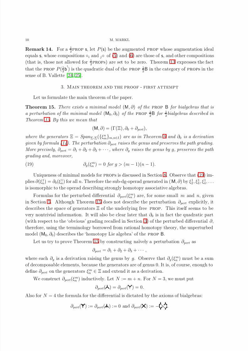
Theorem 15. There exists a minimal model (M, ∂ ) of the prop B for bialgebras that is
a perturbation of the minimal model (M0, ∂ 0) of the prop 12B for 1
2bialgebras described in
Theorem 13 . By this we mean that
(M, ∂ ) = (Γ(Ξ), ∂ 0 + ∂ pert ),
where the generators Ξ = Span Σ-Σ({ξnm}m,n∈I ) are as in Theorem 9 and ∂ 0 is a derivation
given by formula ( 14). The perturbation ∂ pert raises the genus and preserves the path grading.
More precisely, ∂ pert = ∂ 1 + ∂ 2 + ∂ 3 + · · · , where ∂ g raises the genus by g, preserves the path
grading and, moreover,
(19) ∂ g(ξmn ) = 0 for g > (m − 1)(n − 1).
Uniqueness of minimal models for props is discussed in Section 8. Observe that (19) im-
plies ∂ (ξ1n
) = ∂ 0(ξ1n
) for all n. Therefore the sub-dg-operad generated in (M, ∂ ) by ξ12
, ξ13
, ξ14
, . . .
is isomorphic to the operad describing strongly homotopy associative algebras.
Formulas for the perturbed differential ∂ pert (ξmn ) are, for some small m and n, given
in Section 5. Although Theorem 15 does not describe the perturbation ∂ pert explicitly, it
describes the space of generators Ξ of the underlying free prop. This itself seems to be
very nontrivial information. It will also be clear later that ∂ 0 is in fact the quadratic part
(with respect to the ‘obvious’ grading recalled in Section 3) of the perturbed differential ∂ ,
therefore, using the terminology borrowed from rational homotopy theory, the unperturbed
model (M0, ∂ 0) describes the ‘homotopy Lie algebra’ of the prop B.
Let us try to prove Theorem 15 by constructing naıvely a perturbation ∂ pert as
∂ pert = ∂ 1 + ∂ 2 + ∂ 3 + · · · ,
where each ∂ g is a derivation raising the genus by g. Observe that ∂ g(ξmn ) must be a sum
of decomposable elements, because the generators are of genus 0. It is, of course, enough to
define ∂ pert on the generators ξmn ∈ Ξ and extend it as a derivation.
We construct ∂ pert (ξmn ) inductively. Let N := m + n. For N = 3, we must put
∂ pert ( ) = ∂ pert ( ) = 0.
Also for N = 4 the formula for the differential is dictated by the axioms of bialgebras:
∂ pert ( ) := ∂ pert ( ) := 0 and ∂ pert ( ) := − d d .

8/3/2019 Martin Markl- A Resolution (Minimal Model) of the PROP for Bialgebras
http://slidepdf.com/reader/full/martin-markl-a-resolution-minimal-model-of-the-prop-for-bialgebras 11/31
MINIMAL MODEL OF THE PROP FOR BIALGEBRAS 11
For N = 5 we put
∂ pert ( ) = ∂ pert ( ) := 0;
∂ pert ( ) and ∂ pert ( ) are given by formulas
∂ pert ( ) := ( ⊗ )◦σ(2, 2)◦( ⊗ − ⊗ ) − ( ⊗ + ⊗ )◦σ(3, 2)◦( ⊗ ⊗ ),(20)
∂ pert ( ) := ( ⊗ − ⊗ )◦σ(2, 2)◦( ⊗ ) + ( ⊗ ⊗ )◦σ(2, 3)◦( ⊗ + ⊗ ).(21)
In the above displays, σ(2, 2) is the same as in (8),
(22) σ(3, 2) :=
1 2 3 4 5 61 4 2 5 3 6
=
•
•
•
•
•
•
•
•
•
•
•
•
¨ ¨ r r d
with our usual convention that the ‘flow diagrams’ should be read from the bottom to the
top, and σ(3, 2) := σ(2, 3)−1
. Higher terms of the perturbed differential can be constructedby the standard homological perturbation theory as follows.
Suppose we have already constructed ∂ pert (ξuv ) for all u + v < N and fix some m and n
such that m + n = N > 5. We are looking for ∂ pert (ξmn ) of the form
(23) ∂ pert (ξmn ) = ∂ 1(ξm
n ) + ∂ 2(ξmn ) + ∂ 3(ξm
n ) + · · ·
where gen(∂ g(ξmn )) = g. Condition (∂ 0 + ∂ pert )
2(ξmn ) = 0 can be rewritten as
s+t=g
∂ s∂ t(ξmn ) = 0 for each g ≥ 1.
We must therefore find inductively elements ∂ g(ξmn ), g ≥ 1, solving the equation
(24) ∂ 0∂ g(ξmn ) = −
s+t=gt<g
∂ s∂ t(ξmn ).
Observe that the right-hand side of (24) makes sense, because ∂ t(ξmn ) is a combination
of ξuv ’s with u + v < N , therefore ∂ s∂ t(ξm
n ) has already been defined. To verify that the
right-hand side of (24) is a ∂ 0-cycle is also easy:
∂ 0(−s+t=gt<g
∂ s∂ t(ξmn )) = −
s+t=gt<g
∂ 0∂ s∂ t(ξmn ) =
s+t=gt<g
a+b=sb<s
∂ a∂ b∂ t(ξmn )
= 1≤i≤g
∂ i( k+l=g−i
∂ k∂ l(ξm
n
)) = 0.
The degree of the right-hand side of (24) is N − 5, which is a positive number, by
our assumption N > 5. This implies that (24) has a solution, because (Γ(Ξ), ∂ 0) is, by
Theorem 13, ∂ 0-acyclic in positive dimensions.
There is however a serious flaw in the above proof: there is no reason to assume that
the sum (23) is finite, that is, that the right-hand side of (24) is trivial for g sufficiently
large!!! This convergence problem can be fixed by finding subspaces F (m, n) ⊂ Γ(Ξ)(m, n)
satisfying the properties listed in the following definition.
Definition 16. The collection F of subspaces F (m, n) ⊂ Γ(Ξ)(m, n) is friendly if

8/3/2019 Martin Markl- A Resolution (Minimal Model) of the PROP for Bialgebras
http://slidepdf.com/reader/full/martin-markl-a-resolution-minimal-model-of-the-prop-for-bialgebras 12/31
12 M. MARKL
(i) for each m and n, there exists a constant C m,n such that F (m, n) does not contain
elements of genus > C m,n,
(ii) F is stable under all derivations (not necessary differentials) ω satisfying ω(Ξ) ⊂ F ,(iii) ∂ 0(Ξ) ⊂ F , d d ∈ F (2, 2), the right-hand side of ( 20 ) belongs to F (2, 3) and the
right-hand side of ( 21) belongs to F (3, 2), and
(iv) F is ∂ 0-acyclic in positive degrees.
Observe that (ii) with (iii) imply that F is ∂ 0-stable, therefore (iv) makes sense. Observe
also that we do not demand F (m, n) to be Σm-Σn invariant.
Suppose we are given such a friendly collection. We may then, in the above naıve proof,
assume inductively that
(25) ∂ pert (ξmn ) ∈ F (m, n).
Indeed, (25) is satisfied for m + n = 3, 4, 5, by (iii). Condition (ii) guarantees that the right-
hand side of (24) belongs to F (m, n), while (iv) implies that (24) can be solved in F (m, n).
Finally, (i) guarantees, in the obvious way, the convergence.
In this paper, we use the friendly collection S ⊂ Γ(Ξ) of special elements, introduced in
Section 4. The collection S is generated by the free non-Σ 12
prop Γ 12
(Ξ), see Remark 11, by
a suitably restricted class of compositions that naturally generalize those involved in d d .
Another possible choice was proposed in [15], namely the friendly collection defined by
F (m, n) := {f ∈ Γ(Ξ); pth(f ) = mn}.
This choice is substantially bigger than the collection of special elements and contains
‘strange’ elements, such as
∈ F (2, 2)
which we certainly do not want to consider. We believe that special elements are, in a
suitable sense, the smallest possible friendly collection.
Properties of special elements are studied in Sections 6 and 7. Section 9 then contains a
proof of Theorem 15.
4. Special elements
We introduce, in Definition 23, special elements in arbitrary free props. We need first
the following:
Definition 17. For k, l ≥ 1 and 1 ≤ i ≤ kl, let σ(k, l) ∈ Σkl be the permutation given by
σ(i) := k(i − 1 − (s − 1)l) + s,
where s is such that (s−1)l < i ≤ sl. We call permutations of this form special permutations.

8/3/2019 Martin Markl- A Resolution (Minimal Model) of the PROP for Bialgebras
http://slidepdf.com/reader/full/martin-markl-a-resolution-minimal-model-of-the-prop-for-bialgebras 13/31
MINIMAL MODEL OF THE PROP FOR BIALGEBRAS 13
To elucidate the nature of these permutations, suppose we have associative algebras
U 1, . . . , U k. The above permutation is exactly the permutation used to define the induced
associative algebra structure on the product
(U 1 ⊗ · · · ⊗ U k) ⊗ · · · ⊗ (U 1 ⊗ · · · ⊗ U k) /l-times/,
that is, the permutation which takes
(u11 ⊗ u1
2 ⊗ · · · ⊗ u1k) ⊗ (u2
1 ⊗ u22 ⊗ · · · ⊗ u2
k) ⊗ · · · ⊗ (ul1 ⊗ ul
2 ⊗ · · · ⊗ ulk)
to
(u11 ⊗ u2
1 ⊗ · · · ⊗ ul1) ⊗ (u1
2 ⊗ u22 ⊗ · · · ⊗ ul
2) ⊗ · · · ⊗ (u1k ⊗ u2
k ⊗ · · · ⊗ ulk).
Example 18. We have already seen examples of special permutations: the permutation
σ(2, 2) in (8) and the permutation σ(3, 2) in (22). Observe that, for arbitrary k, l ≥ 1,
σ(k, 1) = 1Σk, σ(1, l) = 1Σl
and σ(k, l) = σ(l, k)−1.
Special elements are defined using a special class of compositions defined as follows.
Definition 19. Let P be an arbitrary prop. Let k, l ≥ 1, a1, . . . , al ≥ 1, b1, . . . , bk ≥ 1,
A1, . . . , Al ∈ P(ai, k) and B1, . . . , Bk ∈ P(l, b j ). Then define the (k, l)-fraction
A1 · · · Al
B1 · · · Bk
:= (A1 ⊗ · · · ⊗ Al) ◦ σ(k, l) ◦ (B1 ⊗ · · · ⊗ Bk) ∈ P(a1 + · · · + al, b1 + · · · + bk).
Example 20. If k = 1 or l = 1, the (k, l)-fractions give the ‘operadic’ compositions:
A1 ⊗ · · · ⊗ Al
B1= (A1 ⊗ · · · ⊗ Al) ◦ B1 and
A1
B1 ⊗ · · · ⊗ Bk= A1 ◦ (B1 ⊗ · · · ⊗ Bk).
We are going to use ‘dummy variables,’ that is, for instance, A ∈ P(∗, n) for a fixed
n ≥ 1 means that A ∈ P(m, n) for some m ≥ 1.
Example 21. For a , b ∈ P(∗, 2) and c , d ∈ P(2, ∗),
a b
c d= ( a ⊗ b ) ◦ σ(2, 2) ◦ ( c ⊗ d ) =
dc
ba d d .
Similarly, forx
,y
∈ P(∗, 3) andz
,u
,v
∈ P(2, ∗),
x y
z u v= ( x ⊗ y ) ◦ σ(3, 2) ◦ ( z ⊗ u ⊗ v ) =
vuz
yx
¨ ¨ ¨ r r r d d .
If P is a dg-prop with differential ∂ , then it easily follows from Definition 19 that
∂
A1 · · · Al
B1 · · · Bk
=
1≤i≤l
(−1)deg(A1)+···+deg(Ai−1)A1 · · · ∂Ai · · · Al
B1 · · · · · · Bk
+ 1≤ j≤k
(−1)deg(A1)+···+deg(Al)+deg(B1)+···+deg(Bj−1)A1 · · · · · · Al
B1 · · · ∂B j · · · Bk
.

8/3/2019 Martin Markl- A Resolution (Minimal Model) of the PROP for Bialgebras
http://slidepdf.com/reader/full/martin-markl-a-resolution-minimal-model-of-the-prop-for-bialgebras 14/31
14 M. MARKL
Suppose that the prop P is free, therefore the genus of monomials of P is defined. It is
clear that, under the notation of Example 21,
gen
a b
c d
= 1 + gen( a ) + gen( b ) + gen( c ) + gen( d )
and also that
gen
x y
z u v
= 2 + gen( x ) + gen( y ) + gen( z ) + gen( u ) + gen( v ).
The following lemma generalizes the above formulas.
Lemma 22. Let P be a free prop. Then the genus of the (k, l)-fraction is given by
gen
A1 · · · Al
B1 · · · Bk
= (k − 1)(l − 1) +
l1
gen(Ai) +k1
gen(B j).
Proof. A straightforward and easy verification.
Definition 23. Let us define the collection S ⊂ Γ(Ξ) of special elements to be the smallest
collection of linear subspaces S(m, n) ⊂ Γ(Ξ)(m, n) such that:
(i) 11 ∈ S(1, 1) and all generators ξmn ∈ Ξ belongs to S, and
(ii) if k, l ≥ 1 and A1, . . . , Al, B1, . . . , Bk ∈ S, then
A1 · · · Al
B1 · · · Bk
∈ S.
Remark 24. One may introduce special props as objects similar to props, but for which
only compositions used in the definition of special elements (i.e. the ‘fractions’) are allowed.
The collection S ⊂ Γ(Ξ) would then be the free special prop generated by Ξ.
Example 25. Let the boxes denote arbitrary special elements. Then the elements
and
¡ e
are also special, while the elements
and e ¡
are not special. As an exercise, we recommend calculating the genera of these composed
elements in terms of the genera of individual boxes. Other examples of special elements can
be found in Section 5.
The following lemma states that the path grading of special elements from S(m, n)
equals mn.
8/3/2019 Martin Markl- A Resolution (Minimal Model) of the PROP for Bialgebras
http://slidepdf.com/reader/full/martin-markl-a-resolution-minimal-model-of-the-prop-for-bialgebras 15/31
MINIMAL MODEL OF THE PROP FOR BIALGEBRAS 15
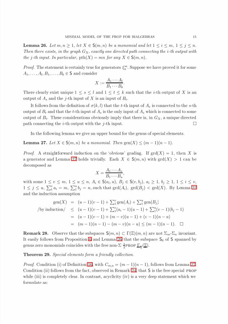
Lemma 26. Let m, n ≥ 1, let X ∈ S(m, n) be a monomial and let 1 ≤ i ≤ m, 1 ≤ j ≤ n.
Then there exists, in the graph GX, exactly one directed path connecting the i-th output with
the j-th input. In particular, pth(X ) = mn for any X ∈ S(m, n).
Proof. The statement is certainly true for generators ξmn . Suppose we have proved it for some
A1, . . . , Al, B1, . . . , Bk ∈ S and consider
X :=A1 · · · Al
B1 · · · Bk
.
There clearly exist unique 1 ≤ s ≤ l and 1 ≤ t ≤ k such that the i-th output of X is an
output of As and the j-th input of X is an input of Bt.
It follows from the definition of σ(k, l) that the t-th input of As is connected to the s-th
output of Bt and that the t-th input of As is the only input of As which is connected to someoutput of Bt. These considerations obviously imply that there is, in GX , a unique directed
path connecting the i-th output with the j-th input.
In the following lemma we give an upper bound for the genus of special elements.
Lemma 27. Let X ∈ S(m, n) be a monomial. Then gen(X ) ≤ (m − 1)(n − 1).
Proof. A straightforward induction on the ‘obvious’ grading. If grd(X ) = 1, then X is
a generator and Lemma 27 holds trivially. Each X ∈ S(m, n) with grd(X ) > 1 can be
decomposed as
X = A1 · · · Av
B1 · · · Bu
,
with some 1 ≤ v ≤ m, 1 ≤ u ≤ n, Ai ∈ S(ai, u), B j ∈ S(v, b j), ai ≥ 1, b j ≥ 1, 1 ≤ i ≤ v,
1 ≤ j ≤ u,v
1 ai = m,u
1 b j = n, such that grd(Ai), grd(B j ) < grd(X ). By Lemma 22
and the induction assumption
gen(X ) = (u − 1)(v − 1) +v
1 gen(Ai) +u
1 gen(B j )
/by induction/ ≤ (u − 1)(v − 1) +v
1(ai − 1)(u − 1) +u
1(v − 1)(b j − 1)
= (u − 1)(v − 1) + (m − v)(u − 1) + (v − 1)(n − u)
= (m − 1)(n − 1) − (m − v)(n − u) ≤ (m − 1)(n − 1).
Remark 28. Observe that the subspaces S(m, n) ⊂ Γ(Ξ)(m, n) are not Σm-Σn invariant.
It easily follows from Proposition 6 and Lemma 26 that the subspace S0 of S spanned by
genus zero monomials coincides with the free non-Σ 12
prop Γ 12
(Ξ).
Theorem 29. Special elements form a friendly collection.
Proof. Condition (i) of Definition 16, with C m,n = (m − 1)(n − 1), follows from Lemma 27.
Condition (ii) follows from the fact, observed in Remark 24, that S is the free special prop
while (iii) is completely clear. In contrast, acyclicity (iv) is a very deep statement which we
formulate as:
8/3/2019 Martin Markl- A Resolution (Minimal Model) of the PROP for Bialgebras
http://slidepdf.com/reader/full/martin-markl-a-resolution-minimal-model-of-the-prop-for-bialgebras 16/31
16 M. MARKL
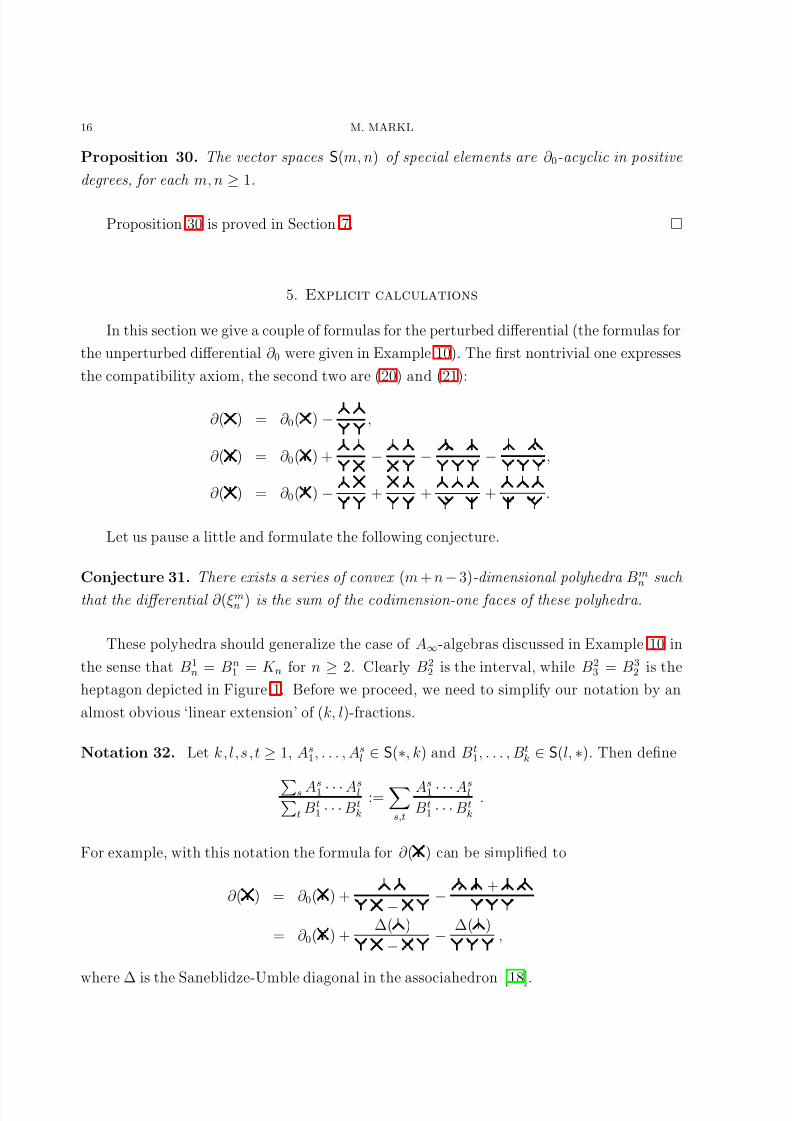
Proposition 30. The vector spaces S(m, n) of special elements are ∂ 0-acyclic in positive
degrees, for each m, n ≥ 1.
Proposition 30 is proved in Section 7.
5. Explicit calculations
In this section we give a couple of formulas for the perturbed differential (the formulas for
the unperturbed differential ∂ 0 were given in Example 10). The first nontrivial one expresses
the compatibility axiom, the second two are (20) and (21):
∂ ( ) = ∂ 0( ) − ,
∂ ( ) = ∂ 0( ) + − − − ,
∂ ( ) = ∂ 0( ) − + + + .
Let us pause a little and formulate the following conjecture.
Conjecture 31. There exists a series of convex (m + n − 3)-dimensional polyhedra Bmn such
that the differential ∂ (ξmn ) is the sum of the codimension-one faces of these polyhedra.
These polyhedra should generalize the case of A∞-algebras discussed in Example 10 in
the sense that B1n = Bn
1 = K n for n ≥ 2. Clearly B22 is the interval, while B2
3 = B32 is the
heptagon depicted in Figure 1. Before we proceed, we need to simplify our notation by an
almost obvious ‘linear extension’ of (k, l)-fractions.
Notation 32. Let k,l,s,t ≥ 1, As1, . . . , As
l ∈ S(∗, k) and Bt1, . . . , Bt
k ∈ S(l, ∗). Then define
s As1 · · · Aslt Bt
1 · · · Btk
:=
s,t
As1 · · · Asl
Bt1 · · · Bt
k
.
For example, with this notation the formula for ∂ ( ) can be simplified to
∂ ( ) = ∂ 0( ) +−
−+
= ∂ 0( ) +∆( )
−−
∆( ),
where ∆ is the Saneblidze-Umble diagonal in the associahedron [18].

8/3/2019 Martin Markl- A Resolution (Minimal Model) of the PROP for Bialgebras
http://slidepdf.com/reader/full/martin-markl-a-resolution-minimal-model-of-the-prop-for-bialgebras 17/31
MINIMAL MODEL OF THE PROP FOR BIALGEBRAS 17
•
•
• •
•
•
•
d d
d
r r r r r r ¨ ¨ ¨ ¨
¨ ¨
Figure 1. Heptagon B23 .
The next term is
∂ ( ) = ∂ 0( ) − − + +
+− − −
−− − −
−+
++
−+ +
+ +.
Observe that the last term of the above equation is
−∆(3)( )
∆(3)( ),
where ∆(3)(−) := (∆⊗11)∆(−) denotes the iteration of the Saneblidze-Umble diagonal which
is coassociative on and (see [13]). The corresponding 3-dimensional polyhedron B33 is
shown in Figure 2.

8/3/2019 Martin Markl- A Resolution (Minimal Model) of the PROP for Bialgebras
http://slidepdf.com/reader/full/martin-markl-a-resolution-minimal-model-of-the-prop-for-bialgebras 18/31
18 M. MARKL
portaturad astra
ornatuscorona
••
• ••••••
••• •
••
••••••••
•••
•••
•••••••••
•
•
••
•
•
¡ ¡
¡ ¡
¡ ¡
¡ ¡ e e
e e
e e
e e d d
d d
d d
d d
d d
d d
d d
¨ ¨ ¨ ¨ ¨ &
& &
&
&
d d
d
d d d
d d
d d
d d
d d
r r r r r
e e
e
e e e
e e
r r r r r
¨ ¨ ¨ ¨ ¨ & &
& &
&
¡ ¡
¡ ¡
¡ ¡
¡ ¡
d d
d d
d d
d d
d d
d d
d d
d d
d d
d d
Figure 2. The plane projection of 3-dimensional polyhedron B33 from one of
its square faces. Polyhedron B33 has 30 2-dimensional faces (8 heptagons and
22 squares), 72 edges and 44 vertices.
The relation with the Saneblidze-Umble diagonal ∆ is even more manifest in the formula
∂ ( ) = ∂ 0( ) ++ +
++
− +
++ + − − −
= ∂ 0( ) +∆( )
+ ++
∆( )
− ++
∆( ).
The corresponding B24 is shown in Figure 3.
6. Calculus of special elements
This section provides a preparatory material for the proof of the ∂ 0-acyclicity of the
space S(m, n) given in Section 7. As in the proof of Lemma 27, each monomial X ∈ S(m, n)
is represented as
(26) X =A1 · · · Av
B1 · · · Bu
,
for 1 ≤ v ≤ m, 1 ≤ u ≤ n, Ai ∈ S(ai, u), B j ∈ S(v, b j ), with
v1 ai = m and
u1 b j = n.
Very crucially, representation (26) is not unique, as illustrated in the following example.

8/3/2019 Martin Markl- A Resolution (Minimal Model) of the PROP for Bialgebras
http://slidepdf.com/reader/full/martin-markl-a-resolution-minimal-model-of-the-prop-for-bialgebras 19/31
MINIMAL MODEL OF THE PROP FOR BIALGEBRAS 19
•
••
••••••
•••••••••
•••••••••
• ••
•
•
d
d d
d d
d d
d d
d d
d d
d d
d d
d d
d
d d
d
d d d
d d
d d
d d
d
d d d
d d
d d
d d
d
e e e ¡
¡ ¡
¡ ¡ ¡
e e e
e e e ¡
¡ ¡
d d d d
d d
Figure 3. The plane projection of 3-dimensional polyhedron B24 . It has 32
vertices, 51 edges and 21 two-dimensional faces (3 pentagons, 5 heptagons and13 squares).
Example 33. It is easy to verify that
(27) = .
Therefore, the element X ∈ S(2, 3) above can be either represented as
X =A1A2
B1B2,
with A1 = A2 = ∈ S(1, 2),
B1 = ∈ S(2, 2)
and B2 = ∈ S(2, 1), or as
X =A′1 A′
2
B′1B′
2B′3
,
with
A′1 = A′
2 = ∈ S(1, 3)
and B′1 = B′
2 = B′3 = ∈ S(2, 1). Of a bit different nature is the relation
(28) =

8/3/2019 Martin Markl- A Resolution (Minimal Model) of the PROP for Bialgebras
http://slidepdf.com/reader/full/martin-markl-a-resolution-minimal-model-of-the-prop-for-bialgebras 20/31
20 M. MARKL
or a similar one
(29) = ,
where is an arbitrary element of S(2, 2).
It follows from the above remarks that
(30) S(m, n) = Span (ξmn ) ⊕
M
S(a1, u) ⊗ · · · ⊗ S(av, u) ⊗ S(v, b1) ⊗ · · · ⊗ S(v, bu)/R(m, n)
where
M = {1 ≤ v ≤ m, 1 ≤ u ≤ n, (v, u) = (1, n), (m, 1) andv
1 ai = m,u
1 b j = n}
and R(m, n) accounts for the non-uniqueness of presentation (26). Observe that if R(m, n)
were trivial, then the ∂ 0-acyclicity of S(m, m) would follow immediately from the Kunneth
formula and induction.
Example 34. We have
S(2, 2) ∼= Span (ξ22) ⊕ [S(2, 1) ⊗ S(1, 2)] ⊕ [S(1, 2) ⊗ S(1, 2) ⊗ S(2, 1) ⊗ S(2, 1)]
∼= Span ( ) ⊕ Span ( ) ⊕ Span
,
the relations R(2, 2) are trivial. On the other hand, the left-hand side of (28) represents an
element of S(3, 3) by
⊗ ⊗ ⊗ ⊗ ∈ S(2, 3) ⊗ S(1, 3) ⊗ S(2, 1) ⊗ S(2, 1) ⊗ S(2, 1),
while the right-hand side of (28) represents the same element by
⊗ ⊗ ⊗ ⊗ ∈ S(1, 2) ⊗ S(1, 2) ⊗ S(1, 2) ⊗ S(3, 2) ⊗ S(3, 1).
Therefore R(3, 3) must contain a relation that identifies these two elements.
Let us describe the space of relations R. Suppose that s, t ≥ 1, c1, . . . , cs, d1, . . . , dt ≥ 1
are natural numbers and let (c;d) denote the array (c1, . . . , cs; d1, . . . , dt). A crucial role in
the following definition will be played by a matrix
(31) C = (C ij) 1≤i≤t1≤j≤s
with entries C ij ∈ S(di, c j). Finally, let
X =A1 · · · Av
B1 · · · Bu
be a monomial as in (26).

8/3/2019 Martin Markl- A Resolution (Minimal Model) of the PROP for Bialgebras
http://slidepdf.com/reader/full/martin-markl-a-resolution-minimal-model-of-the-prop-for-bialgebras 21/31
MINIMAL MODEL OF THE PROP FOR BIALGEBRAS 21
Definition 35. Element X is called (c;d)-up-reducible if u = c1 + · · · + cs, v = t and
(32) Ai =Ai1 · · · Aidi
C i1 · · · C is
for some Aib ∈ S(∗, s), 1 ≤ i ≤ t, 1 ≤ b ≤ di, where C ij are entries of a matrix as in ( 31).
Dually, X is called (c;d)-down-reducible if v = d1 + · · · + dt, u = s and
(33) B j =C 1 j · · · C tj
B1 j · · · Bcj j
for some Baj ∈ S(t, ∗), 1 ≤ j ≤ s, 1 ≤ a ≤ c j, again with C = (C ij) as in ( 31). We
denote by Up(c; d) (resp. Dw(c;d)) the subspace spanned by all (c;d)-(resp. down) -reducible
monomials.
Proposition 36. The spaces Up(c; d) and Dw(c; d) are isomorphic. The isomorphism is
given by the identification of the up-reducible element
A11···A1d1
C 11···C 1s
A21···A2d2
C 21···C 2s· · ·
At1···Atdt
C t1···C ts
B11 · · · Bc11 B12 · · · Bc22 · · · B1s · · · Bcss
with the down-reducible element
A11 · · · A1d1 A21 · · · A2d2 · · · At1 · · · Atdt
C 11···C t1B11···Bc
1
1
C 12···C t2B12···Bc
2
2
· · · C 1s···C tsB1s···Bcss
.
Relations R in ( 30 ) are generated by the above identifications.
Proof. The proof follows from analyzing the underlying graphs.
We call the relations described in Proposition 36 the (c;d)-relations . These relations are
clearly compatible with the differential ∂ 0 and do not change the genus. They are trivial if
d j = ci = 1, for all i, j.
Example 37. Equation (27) of Example 33 is an equality of two (2, 1; 1, 1)-reducible ele-
ments with A11 = A21 = , B11 = B21 = B12 = and the matrix (31) given by
C =
1111
.
Equation (28) of Example 33 is an equality between two (2, 1; 2, 1)-reducible elements with
A11 = A12 = A21 = , B11 = B21 = B12 = and
C =
11
.
We leave it as an exercise to interpret also (29) in terms of (c;d)-relations.

8/3/2019 Martin Markl- A Resolution (Minimal Model) of the PROP for Bialgebras
http://slidepdf.com/reader/full/martin-markl-a-resolution-minimal-model-of-the-prop-for-bialgebras 22/31
22 M. MARKL
Example 38. Let us write presentation (30) for S(2, 3). Of course, S(2, 3) = S0(2, 3) ⊕
S1(2, 3) ⊕S2(2, 3), where the subscript denotes the genus. Then S0(2, 3) is represented as the
quotient of
Span (ξ23) ⊕ [S0(2, 2)⊗S(1, 1)⊗S(1, 2)] ⊕ [S(2, 1)⊗S(1, 3)] ⊕ [S0(2, 2)⊗S(1, 2)⊗S(1, 1)] ∼=
∼= Span ( ) ⊕ Span
11
⊕ Span
⊕ Span
11
,
where is an arbitrary element of S0(1, 3) and is an element of S0(2, 2), modulo relations
R(2, 3) that identify the up-(2; 1)-reducible element
11∈ Span
11
with the down-(2; 1)-reducible element
∈ Span
and identify the up-(2; 1)-reducible element
11∈ Span
11
with the down-(2; 1)-reducible element
∈ Span
.
With the obvious similar notation, S1(2, 3) is the quotient of
Span
⊕ Span
11
⊕ Span
⊕ Span
11
,
where again ∈ S0(2, 2) is an arbitrary element, modulo relations R(2, 3) that identify the
up-(1, 1; 2)-reducible generator of the second summand with
∈ Span
and the up-(1, 1; 2)-reducible generator of the fourth summand with
∈ Span
.
Finally, S2(2, 3) is the quotient of
Span
1111
⊕ Span
⊕ Span
1111
modulo R(2, 3) identifying the up-(2, 1; 1, 1)-reducible element
∈ Span

8/3/2019 Martin Markl- A Resolution (Minimal Model) of the PROP for Bialgebras
http://slidepdf.com/reader/full/martin-markl-a-resolution-minimal-model-of-the-prop-for-bialgebras 23/31
MINIMAL MODEL OF THE PROP FOR BIALGEBRAS 23
with the generator of the first summand, and the up-(1 , 2; 1, 1)-reducible element
∈ Span
with the generator of the last summand.
Example 38 shows that presentation (30) is not economical. Moreover, we do not need
to delve into the structure of S0(m, n) because we already know that this piece of S(m, n),
isomorphic to the free non-Σ 12
prop Γ 12
(Ξ), is ∂ 0-acyclic, see Remarks 11, 28 and Theorem 9.
So we will work with the reduced form of presentation (30):
(34) S(m, n) = S0(m, n) ⊕
N
S(a1, u) ⊗ · · · ⊗ S(av, u) ⊗ S(v, b1) ⊗ · · · ⊗ S(v, bu)/Q(m, n)
where
(35) N := M ∩ {v ≥ 2, u ≥ 2} = {2 ≤ v ≤ m, 2 ≤ u ≤ n, andv
1 ai = m,u
1 b j = n}
and Q(m, n) ⊂ R(m, n) is the span of (c1, . . . , cs; d1, . . . , dt)-relations with s, t ≥ 2.
Example 39. We have the following reduced representations:
S(2, 2) = S0(2, 2) ⊕ Span
and(36)
S1(2, 3) = Span ⊕ Span , where ∈ S0(2, 2).
The reduced presentation of S2(2, 3) is the same as the unreduced one given in Example 38.
We conclude that
S(2, 3) ∼= S0(2, 3) ⊕ S0(2, 2) ⊕ S0(2, 2) ⊕ S0(1, 3)⊗2.
This, by the way, immediately implies the ∂ 0-acyclicity of S(2, 3).
7. Acyclicity of the space of special elements
The proof of the ∂ 0-acyclicity, in positive dimensions, of S(m, n) is given by induction
on K := m · n. The acyclicity is trivial for K ≤ 2. Indeed, there are only three spaces to
consider, namely S(1, 1) = Span (11), S(1, 2) = Span ( ) and S(2, 1) = Span ( ). All these
spaces are concentrated in degree zero and have trivial differential.
The acyclicity is, in fact, obvious also for K = 3 because S(1, 3) = S0(1, 3) and S(3, 1) =
S0(3, 1) coincide with their tree parts. For K = 4 we have two ‘easy’ cases, S(4, 1) = S0(4, 1)
and S(1, 4) = S0(1, 4), while the acyclicity of S(2, 2) follows from presentation (36).
Suppose we have proved the ∂ 0-acyclicity of all S(k, l) with k · l < K . Let us express the
reduced presentation (34) as the short exact sequence
(37) 0 −→ Q(m, n) −→ L(m, n) ⊕ S0(m, n) −→ S(m, n) −→ 0,

8/3/2019 Martin Markl- A Resolution (Minimal Model) of the PROP for Bialgebras
http://slidepdf.com/reader/full/martin-markl-a-resolution-minimal-model-of-the-prop-for-bialgebras 24/31
24 M. MARKL
where we denoted
L(m, n) := N
S(a1, u) ⊗ · · · ⊗ S(av, u) ⊗ S(v, b1) ⊗ · · · ⊗ S(v, bu)
with N defined in (35). It follows from the Kunneth formula and induction that L(m, n)
is ∂ 0-acyclic while the acyclicity of S0(m, n) ∼= Γ 12
(Ξ) was established in Remark 11. Short
exact sequence (37) then implies that it is in fact enough to prove that the space of relations
Q(m, n) is ∂ 0-acyclic for any m, n ≥ 1. This would clearly follow from the following claim.
Claim 40. For any w ∈ L(m, n) such that ∂ 0(w) ∈ Q(m, n), there exists z ∈ Q(m, n) such
that ∂ 0(z) = ∂ 0(w).
Proof. It follows from the nature of relations in the reduced presentation ( 34) that
(38) ∂ 0(w) =(c;d)
u(c;d)↑ − u(c;d)
↓ ,
where the summation runs over all (c; d) = (c1, . . . , cs; d1, . . . , dt) with s, t ≥ 2, and u(c;d)↑
(resp. u(c;d)↓ ) is an (c;d)-up (resp. down) reducible element such that u
(c;d)↑ −u
(c;d)↓ ∈ Q(m, n).
The idea of the proof is to show that there exists, for each (c;d), some (c;d)-up-reducible
z(c;d)↑ and some (c;d)-down-reducible z
(c;d)↓ such that z(c;d) := z
(c;d)↑ −z
(c;d)↓ belongs to Q(m, n)
and
(39) u(c;d)↑ − u
(c;d)↓ = ∂ 0(z(c;d)).
Then z :=
(c;d) z(c;d)
will certainly fulfill ∂ 0(z) = ∂ 0(w). We will distinguish five types of (c; d)’s. The first four types are easy to handle; the last type is more intricate.
Type 1: All d1, . . . , dt are ≥ 2 and all c1, . . . , cs are arbitrary. In this case u(c;d)↑ is of the
form
(40)A1 · · · At
B1 · · · Bu
with
Ai =Ai1 · · · Aidi
C i1 · · · C is
as in (32). It follows from the definition that ∂ 0 cannot create (k, l)-fractions with k, l ≥
2. Therefore a monomial as in (40) may occur among monomials forming ∂ 0(y) for somemonomial y if and only if y itself is of the above form. Let z
(c;d)↑ be the sum of all monomials
in w whose ∂ 0-boundary nontrivially contributes to u(c;d)↑ . Let z
(c;d)↓ be the corresponding
(c;d)-down-reducible element. Then clearly u(c;d)↓ = ∂ 0(z
(c;d)↓ ) and (39) is satisfied with
z(c;d) := z(c;d)↑ − z
(c;d)↓ constructed above. In this way, we may eliminate all (c; d)’s of Type 1
from (38).
Type 2: All c1, . . . , ct = 1 and all d1, . . . , ds are arbitrary. In this case u(c;d)↑ is of the
form
(41)A1 · · · At
B1 · · · Bu

8/3/2019 Martin Markl- A Resolution (Minimal Model) of the PROP for Bialgebras
http://slidepdf.com/reader/full/martin-markl-a-resolution-minimal-model-of-the-prop-for-bialgebras 25/31
MINIMAL MODEL OF THE PROP FOR BIALGEBRAS 25
with
(42) Ai =
Ai1 · · · Aidi
C i1 · · · C is ,
where C ij ∈ S(di, 1), for 1 ≤ i ≤ t, 1 ≤ j ≤ s. When di = 1,
Ai = Ai1 ◦ (C i1 ⊗ · · · ⊗ C is),
where C ij ∈ S(1, 1) must be a scalar multiple of 11. We observe that element (41) is (c; d)-up
reducible if and only if Ai is as in (42) where di ≥ 2; if di = 1 then Ai may be arbitrary. We
conclude, as in the previous case, that a monomial of the above form may occur in ∂ 0(y) if
and only if y itself is of the above form. Therefore, by the same argument, we may eliminate
(c; d)’s of Type 2 from (38).
Type 3: All c1, . . . , ct ≥ 2 and d1, . . . , ds are arbitrary. This case is dual to Type 1.
Type 4: All d1, . . . , dt = 1 and c1, . . . , cs are arbitrary. This case is dual to Type 2.
Type 5: The remaining case. This means that 1 ∈ {c1, . . . , cs} but there exist some
c j ≥ 2, and 1 ∈ {d1, . . . , dt} but there exists some di ≥ 2. This is the most intricate case,
because it may happen that, for some monomial y, ∂ 0(y) contains a (c;d)- (up- or down-)
reducible piece although y itself is not (c; d)-reducible. For instance, let
y :=
d d
.
Then ∂ 0(y) contains a (2, 1; 2, 1)-up-reducible piece
d d
though y itself is not (2, 1; 2, 1)-up-reducible. Nevertheless, we see that ∂ 0(y) contains also
d d
which is not reducible. This is in fact a general phenomenon, that is, if ∂ 0(y) contains
a (c;d)-up-reducible piece and if y is not (c;d)-up-reducible, then ∂ 0(y) contains also an
irreducible piece. Therefore such y cannot occur among monomials forming up w in Claim 40.
We conclude that y must also be (c;d)-up-reducible and eliminate it from (38) as in the
previous cases. Down-reducible pieces can be handled similarly. This finishes our proof of
Claim 40.
8/3/2019 Martin Markl- A Resolution (Minimal Model) of the PROP for Bialgebras
http://slidepdf.com/reader/full/martin-markl-a-resolution-minimal-model-of-the-prop-for-bialgebras 26/31
26 M. MARKL
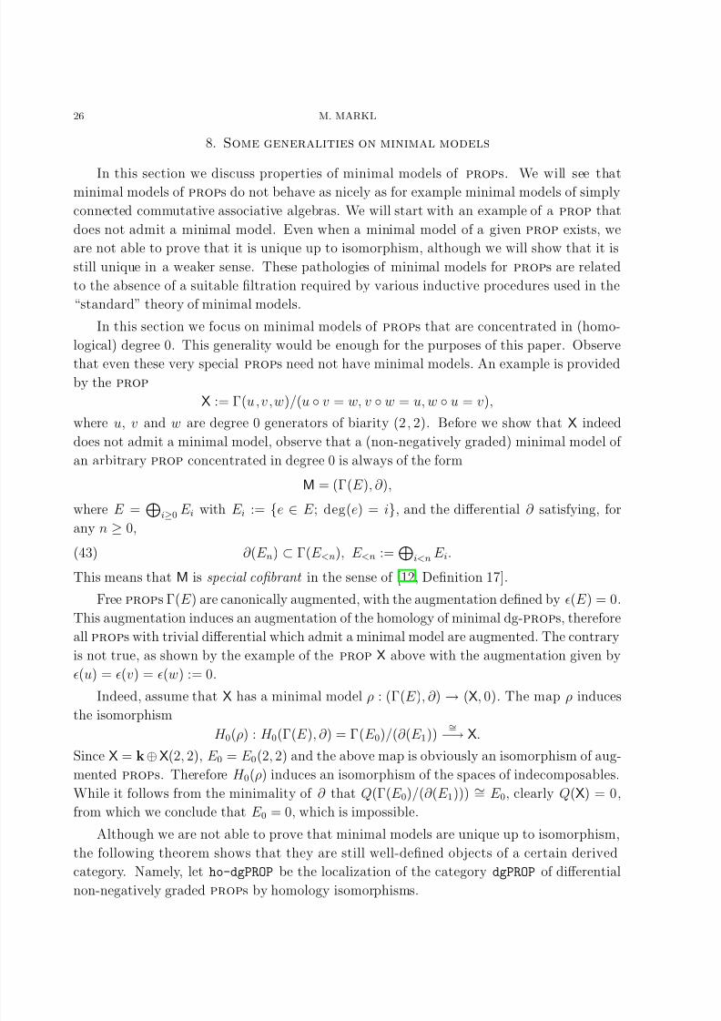
8. Some generalities on minimal models
In this section we discuss properties of minimal models of props. We will see thatminimal models of props do not behave as nicely as for example minimal models of simply
connected commutative associative algebras. We will start with an example of a prop that
does not admit a minimal model. Even when a minimal model of a given prop exists, we
are not able to prove that it is unique up to isomorphism, although we will show that it is
still unique in a weaker sense. These pathologies of minimal models for props are related
to the absence of a suitable filtration required by various inductive procedures used in the
“standard” theory of minimal models.
In this section we focus on minimal models of props that are concentrated in (homo-
logical) degree 0. This generality would be enough for the purposes of this paper. Observe
that even these very special props need not have minimal models. An example is provided
by the prop
X := Γ(u,v,w)/(u ◦ v = w, v ◦ w = u, w ◦ u = v),
where u, v and w are degree 0 generators of biarity (2, 2). Before we show that X indeed
does not admit a minimal model, observe that a (non-negatively graded) minimal model of
an arbitrary prop concentrated in degree 0 is always of the form
M = (Γ(E ), ∂ ),
where E =
i≥0 E i with E i := {e ∈ E ; deg(e) = i}, and the differential ∂ satisfying, for
any n ≥ 0,
(43) ∂ (E n) ⊂ Γ(E <n), E <n :=
i<n E i.
This means that M is special cofibrant in the sense of [12, Definition 17].
Free props Γ(E ) are canonically augmented, with the augmentation defined by ǫ(E ) = 0.
This augmentation induces an augmentation of the homology of minimal dg-props, therefore
all props with trivial differential which admit a minimal model are augmented. The contrary
is not true, as shown by the example of the prop X above with the augmentation given by
ǫ(u) = ǫ(v) = ǫ(w) := 0.
Indeed, assume that X has a minimal model ρ : (Γ(E ), ∂ ) → (X, 0). The map ρ induces
the isomorphismH 0(ρ) : H 0(Γ(E ), ∂ ) = Γ(E 0)/(∂ (E 1))
∼=−→ X.
Since X = k ⊕X(2, 2), E 0 = E 0(2, 2) and the above map is obviously an isomorphism of aug-
mented props. Therefore H 0(ρ) induces an isomorphism of the spaces of indecomposables.
While it follows from the minimality of ∂ that Q(Γ(E 0)/(∂ (E 1))) ∼= E 0, clearly Q(X) = 0,
from which we conclude that E 0 = 0, which is impossible.
Although we are not able to prove that minimal models are unique up to isomorphism,
the following theorem shows that they are still well-defined objects of a certain derived
category. Namely, let ho-dgPROP be the localization of the category dgPROP of differential
non-negatively graded props by homology isomorphisms.

8/3/2019 Martin Markl- A Resolution (Minimal Model) of the PROP for Bialgebras
http://slidepdf.com/reader/full/martin-markl-a-resolution-minimal-model-of-the-prop-for-bialgebras 27/31
MINIMAL MODEL OF THE PROP FOR BIALGEBRAS 27
Proposition 41. Let A be a prop concentrated in degree 0. Then its minimal model (if
exists), considered as an object of the localized category ho-dgPROP, is unique up to isomor-
phism.
Proof. The proposition would clearly be implied by the following statement. Let α : M′ → A
and β : M′′ → A be two minimal models of A. Then there exists a homomorphism h : M′ →
M′′ such that the diagram
M′ M′′
A
E
d d d
©α
h
β
commutes. Such a map h can be constructed by induction. Assume that M′ = (Γ(E ), ∂ ′),
M′′ = (Γ(F ), ∂ ′′) and let h0 : Γ(E 0) → M′′ be an arbitrary lift in the diagram
Γ(E 0) M′′
A
E
d d d
©α|Γ(E0)
h0
β
Suppose we have already constructed, for some n ≥ 1, a homomorphism
hn−1 : Γ(E <n) → M′′,
such that β ◦hn−1 = α|Γ(E <n), where E <n is as in (43). Let us show that hn−1 can be extended
into hn : Γ(E <n+1) → M′′
with the similar property. To this end, fix a k-linear basis Bn of E n and observe that for each e ∈ Bn there exists a solution ωe ∈ M′′ of the equation
(44) ∂ ′′(ωe) = hn−1(∂ ′e).
This follows from the fact that ∂ ′′hn−1(∂ ′e) = hn−1(∂ ′∂ ′e) = 0 which means that the right-
hand side of (44) is a ∂ ′′-cycle, therefore ωe exists by the acyclicity of M′′ in degree n − 1.
Define a linear map rn : E n → M′′ by rn(e) := ωe, for e ∈ Bn. Finally, define a linear
equivariant map rn : E n → M′′ by
rn(f ) :=τ,σ
1
k! l!σ−1rn(σf τ )τ −1,
where f ∈ E n is of biarity (k, l) and the summation runs over all σ ∈ Σk and τ ∈ Σl. It is
easy to verify that the homomorphism hn : Γ(E n) → M′′ determined by hn(f ) := rn(f ) for
f ∈ E n, extends hn−1, and the induction goes on.
By modifying the proof of [12, Lemma 20], one may generalize Proposition 41 to an
arbitrary non-negatively graded prop with trivial differential.
Remark 42. One usually proves that two minimal models connected by a (co)homology
isomorphisms are actually isomorphic. This is for instance true for minimal models of 1-
connected commutative associative dg-algebras [7, Theorem 11.6(iv)], minimal models of
connected dg-Lie algebras [23, Theorem II.4(9)] as well as for minimal models of augmented

8/3/2019 Martin Markl- A Resolution (Minimal Model) of the PROP for Bialgebras
http://slidepdf.com/reader/full/martin-markl-a-resolution-minimal-model-of-the-prop-for-bialgebras 28/31
28 M. MARKL
operads [14, Proposition 3.120]. We do not know whether this isomorphism theorem is true
also for minimal models of props.
However, ‘classical’ isomorphism theorems can still be proved if one imposes some ad-
ditional assumptions on the type of minimal models involved, as illustrated by Theorem 43
below. Let us call a minimal model (Γ(Ξ), ∂ ) of the bialgebra prop B special if the differen-
tial ∂ preserves the subspace of special elements and if it is of the form ∂ = ∂ 0 + ∂ pert , where
∂ 0 is as in (14) and ∂ pert raises the genus.
Theorem 43. Let M′ = (Γ(Ξ), ∂ ′) and M′′ = (Γ(Ξ), ∂ ′′) be two special minimal models for
the bialgebra prop B. Then there exists an isomorphism φ : M′ → M′′ preserving the space
of special elements.
Proof. Let us construct inductively a map φ : (Γ(Ξ), ∂ ′) → (Γ(Ξ), ∂ ′′) of augmented props
which preserves the space of special elements and which is the ‘identity modulo elements
of higher genus.’ By this we mean that φ|Ξ = 11Ξ + η, where the image of the linear map
η : Ξ → Γ(Ξ) consists of special elements of positive genera.
The first step of the inductive construction is easy: we define φ0 : Γ(Ξ0) → Γ(Ξ) by
φ0|Ξ0 := 11Ξ0. Suppose we have already constructed φn−1 : Γ(Ξ<n) → Γ(Ξ). As in the proof
of Proposition 41, one must solve, for each element e of a basis of Ξn, the equation
(45) ∂ ′′ωe = φn−1(∂ ′e).
The right-hand side is a ∂ ′′-cycle, therefore a solution ωe exist by the acyclicity of M′′ in
degree n − 1. But not every solution is good for our purposes. Observe that the right-hand
side of (45) is of the form
φn−1(∂ 0e + ∂ ′pert e) = ∂ 0(e) + ϑe,
where ϑe is a sum of special elements of positive genera. We leave as an exercise to prove
that the ∂ 0-acyclicity of the space of special elements implies, similarly as in the ‘naıve’ proof
of Theorem 15 given in Section 3, that in fact there exists ωe of the form ωe = e + ηe, where
ηe is a sum of special elements of genus > 0. Therefore
φn(e) := ωe = e + ηe, e ∈ Ξn,
defines an extension of φn−1 which preserves special elements and which is the identity
modulo elements of higher genera.
The proof is concluded by showing that every endomorphism φ : Γ(Ξ) → Γ(Ξ) whose
linear part is the identity and which preserves the space of special elements is invertible. We
leave this statement as another exercise to the reader.

8/3/2019 Martin Markl- A Resolution (Minimal Model) of the PROP for Bialgebras
http://slidepdf.com/reader/full/martin-markl-a-resolution-minimal-model-of-the-prop-for-bialgebras 29/31
MINIMAL MODEL OF THE PROP FOR BIALGEBRAS 29
9. Proof of the main theorem and final reflections
Proof of Theorem 15 . We already know from Theorem 29 that the collection S of specialelements is friendly, therefore the inductive construction described in Section 3 gives a per-
turbation ∂ pert = ∂ 1 + ∂ 2 + ∂ 3 + · · · such that
∂ g(ξmn ) ∈ Sg(m, n), for g ≥ 0.
Equation (19) then immediately follows from Lemma 27 while the fact that ∂ pert preserves
the path grading follows from Lemma 26.
It remains to prove that (M, ∂ ) = (Γ(Ξ), ∂ 0 + ∂ pert ) really forms a minimal model of B,
that is, to construct a homology isomorphism from (M, ∂ ) to (B, ∂ = 0). To this end, consider
the homomorphism
ρ : (Γ(Ξ), ∂ 0 + ∂ pert ) → (B, ∂ = 0)
defined, in presentation (7), by
ρ(ξ12) := , ρ(ξ21) := ,
while ρ is trivial on all remaining generators. It is clear that ρ is a well-defined map of
dg-props. The fact that ρ is a homology isomorphism follows from rather deep Corollary 27
of [15]. An important assumption of this Corollary is that ∂ pert preserves the path grading.
This assumption guarantees that the first spectral sequence of [15, Theorem 24] converges
because of the inequalities given in [15, Exercise 21] and recalled here in (9). The proof of
Theorem 15 is finished.
Final reflections and problems. We observed that it is extremely difficult to work with
free props. Fortunately, it turns out that most of classical structures are defined over simpler
objects – operads, 12props or dioperads. In Remark 24 we indicated a definition of special
props for which only compositions given by ‘fractions’ are allowed.
Let us denote by sB the special prop for bialgebras. It clearly fulfills sB(m, n) = k for
all m, n ≥ 1 which means that bialgebras are the easiest objects defined over special props
in the same sense in which associative algebras are the easiest objects defined over non-Σ-
operads (recall that the non-Σ-operad Ass for associative algebras fulfills Ass(n) = k for all
n ≥ 1) and associative commutative algebras are the easiest objects defined over (Σ-)operads
(operad Com fulfills Com (n) = k for all n ≥ 1).
Let us close this paper by summarizing some open problems.
(1) Does there exist a sequence of convex polyhedra Bmn with the properties stated in
Conjecture 31?
(2) What can be said about the minimal model for the prop for “honest” Hopf algebras
with an antipode?
(3) Explain why the Saneblidze-Umble diagonal occurs in our formulas for ∂ .

8/3/2019 Martin Markl- A Resolution (Minimal Model) of the PROP for Bialgebras
http://slidepdf.com/reader/full/martin-markl-a-resolution-minimal-model-of-the-prop-for-bialgebras 30/31
30 M. MARKL
(4) Describe the generating function
f (s, t) := m,n≥1
dim S(m, n)smtn
for the space of special elements.
(5) Give a closed formula for the differential ∂ of the minimal model.
(6) Develop a theory of homotopy invariant versions of algebraic objects over props,
parallel to that of [12] for algebras over operads. We expect that all main results of [12]
remain true also for props, though there might be surprises and unexpected difficulties
related to the combinatorial explosion of props.
(7) What can be said about the uniqueness of the minimal model? Is the minimal model
of an augmented prop concentrated in degree 0 unique up to isomorphism? If not, is at
least a suitable completition of the minimal model unique?
There is a preprint [17] which might contain answers to Problems (1) and (5).
References
[1] B. Enriquez and P. Etingof. On the invertibility of quantization functors. Preprint math.QA/0306212,June 2003.
[2] W.L. Gan. Koszul duality for dioperads. Math. Res. Lett., 10(1):109–124, 2003.[3] M. Gerstenhaber and S.D. Schack. Bialgebra cohomology, deformations, and quantum groups. Proc.
Nat. Acad. Sci. USA, 87:478–481, 1990.[4] S. Halperin and J.D. Stasheff. Obstructions to homotopy equivalences. Adv. in Math., 32:233–279, 1979.[5] M. Kontsevich. An e-mail message to M. Markl, November 2002.
[6] M. Kontsevich and Y. Soibelman. Deformation theory of bialgebras, Hopf algebras and tensor categories.Preprint, March 2002.
[7] D. Lehmann. Theorie Homotopique des Formes Differentielles, volume 54 of Asterisque. Soc. Math.France, 1977.
[8] S. Mac Lane. Natural associativity and commutativity. Rice Univ. Stud., 49(1):28–46, 1963.[9] M. Markl. Deformations and the coherence. Proc. of the Winter School ‘Geometry and Physics,’ Zdıkov,
Bohemia, January 1993, Supplemento ai Rend. Circ. Matem. Palermo, Serie II , 37:121–151, 1994.[10] M. Markl. Cotangent cohomology of a category and deformations. J. Pure Appl. Algebra , 113:195–218,
1996.[11] M. Markl. Models for operads. Comm. Algebra , 24(4):1471–1500, 1996.[12] M. Markl. Homotopy algebras are homotopy algebras. Forum Mathematicum , 16(1):129–160, January
2004. Preprint available as math.AT/9907138.[13] M. Markl and S. Shnider. Associahedra, cellular W-construction and products of A∞-algebras. Preprint
math.AT/0312277, December 2003. To appear in Trans. Amer. Math. Soc.[14] M. Markl, S. Shnider, and J. D. Stasheff. Operads in Algebra, Topology and Physics, volume 96 of
Mathematical Surveys and Monographs. American Mathematical Society, Providence, Rhode Island,2002.
[15] M. Markl and A.A. Voronov. PROPped up graph cohomology. Preprint math.QA/0307081, July 2003.[16] T. Pirashvili. On the Prop corresponding to bialgebras. Preprint 00-089 Universitat Bielefeld, 2000.[17] S. Saneblidze and R. Umble. The biderivative and A∞-bialgebras. Preprint math.AT/0406270, April
2004.[18] S. Saneblidze. and R. Umble. Diagonals on the permutohedra, multiplihedra and associahedra. Preprint
math.AT/0209109, August 2002.[19] S. Saneblidze and R. Umble. The biderivative, matrons and A∞-bialgebras. Preprint, July 2004.[20] B. Shoikhet. A concept of 2
3PROP and deformation theory of (co) associative coalgebras. Preprint
math.QA/0311337, November 2003.

8/3/2019 Martin Markl- A Resolution (Minimal Model) of the PROP for Bialgebras
http://slidepdf.com/reader/full/martin-markl-a-resolution-minimal-model-of-the-prop-for-bialgebras 31/31
MINIMAL MODEL OF THE PROP FOR BIALGEBRAS 31
[21] B. Shoikhet. The CROCs, non-commutative deformations, and (co)associative bialgebras. Preprint math.QA/0306143, June 2003.
[22] B. Shoikhet. An explicit deformation theory of (co)associative bialgebras. Preprint math.QA/0310320,October 2003.
[23] D. Tanre. Homotopie Rationnelle: Modeles de Chen, Quillen, Sullivan , volume 1025 of Lect. Notes in
Math. Springer-Verlag, 1983.[24] B. Vallette. Dualite de Koszul des PROPs. PhD thesis, Universite Louis Pasteur, 2003.[25] B. Vallette. Koszul duality for PROPs. Comptes Rendus Math., 338(12):909–914, June 2004.
E-mail address : [email protected]
Mathematical Institute of the Academy, Zitna 25, 115 67 Prague 1, The Czech Republic