Policy Research Working Paper 5796

Marshallian Externality, Industrial Upgrading, and Industrial Policies

Jiandong JuJustin Yifu Lin

Yong Wang

The World BankDevelopment Economics Vice PresidencySeptember 2011

WPS5796P

ublic

Dis

clos

ure

Aut

horiz

edP

ublic

Dis

clos

ure

Aut

horiz

edP

ublic

Dis

clos

ure

Aut

horiz

edP

ublic

Dis

clos

ure

Aut

horiz

edP

ublic

Dis

clos

ure

Aut

horiz

edP

ublic

Dis

clos

ure

Aut

horiz

edP

ublic

Dis

clos

ure

Aut

horiz

edP

ublic

Dis

clos

ure

Aut

horiz

ed

Produced by the Research Support Team

Abstract

The Policy Research Working Paper Series disseminates the findings of work in progress to encourage the exchange of ideas about development issues. An objective of the series is to get the findings out quickly, even if the presentations are less than fully polished. The papers carry the names of the authors and should be cited accordingly. The findings, interpretations, and conclusions expressed in this paper are entirely those of the authors. They do not necessarily represent the views of the International Bank for Reconstruction and Development/World Bank and its affiliated organizations, or those of the Executive Directors of the World Bank or the governments they represent.

Policy Research Working Paper 5796

A growth model with multiple industries is developed to study how industries evolve as capital accumulates endogenously when each industry exhibits Marshallian externality (increasing returns to scale) and to explain why industrial policies sometimes succeed but sometimes fail. The authors show that, in the long run, the laissez-faire market equilibrium is Pareto optimal when the time discount rate is sufficiently small or sufficiently large. When the time discount rate is moderate, there

This paper is a product of the Development Economics Vice Presidency. It is part of a larger effort by the World Bank to provide open access to its research and make a contribution to development policy discussions around the world. Policy Research Working Papers are also posted on the Web at http://econ.worldbank.org. The authors may be contacted at jdju@ou.edu, justinlin@worldbank.org, and yongwang@ust.hk.

exist multiple dynamic market equilibria with diverse patterns of industrial development. To achieve Pareto efficiency, it would require the government to identify the industry target consistent with the comparative advantage and to coordinate in a timely manner, possibly for multiple times. However, industrial policies may make people worse off than in the market equilibrium if the government picks an industry that deviates from the comparative advantage of the economy.

Marshallian Externality, Industrial Upgrading,and Industrial Policies�

Jiandong Juy, Justin Yifu Linz, Yong Wangx

July 21, 2011

Abstract

A growth model with multiple industries is developed to study howindustries evolve as capital accumulates endogenously when each indus-try exhibits Marshallian externality (increasing returns to scale) and toexplain why industrial policies sometimes succeed but sometimes fail. Theauthors show that, in the long run, the laissez-faire market equilibriumis Pareto optimal when the time discount rate is su¢ ciently small or suf-�ciently large. When the time discount rate is moderate, there existmultiple dynamic market equilibria with diverse patterns of industrial de-velopment. To achieve Pareto e¢ ciency, it would require the governmentto identify the industry target consistent with the comparative advantageand to coordinate in a timely manner, possibly for multiple times. How-ever, industrial policies may make people worse o¤ than in the marketequilibrium if the government picks an industry that deviates from thecomparative advantage of the economy.

Key Words: Marshallian Externality, Industrial Policies, StructuralTransformation, Industrial Upgrading, Economic Growth

JEL Codes: L50, O14, O25, O41

�This paper bene�ts from the discussions with Gene Grossman, Norman Loayza, andAart Kraay. Roula Yazigi provides excellent editorial support. Wang gratefully acknowledgesthe hospitality and �nancial support from the World Bank during his stay in the 2010-2011academic year.

yUniversity of Oklahoma and Tsinghua University. Email Address: jdju@ou.eduzWorld Bank. Email address: justinlin@worldbank.orgxHong Kong University of Science and Technology. Email address: yongwang@ust.hk

1

1 Introduction

This paper studies the role of industrial policies in a growth model with multipleindustries. In the real world, for better or worse, almost all the economieshave adopted and are still adopting various industrial policies.1 Yet the e¤ectof industrial policies is always highly controversial. On the one hand, manyempirical and case studies suggest that industrial policies have mostly failed andthe overall performance of industrial policies is very mixed and insigni�cant;2

but on the other hand, ample research, especially case studies, contends thatindustrial policies and government facilitation are crucially important for most,if not all, of the cases of successful industrial development.3

The main purpose of this paper is to help reconcile these two di¤erent em-pirical facts and views, which tend to convey opposite implications for the desir-ability of industrial policies. More speci�cally, we try to shed some new light onwhy "similar" industrial policies work in some cases but fail in others. Any use-ful discussion on industrial policies must involve the existence of certain marketimperfections. In this paper we will revisit and focus on the issue of Marshal-lian externality, the importance of which is widely recognized in the existingliterature. For example, one in�uential study on coordination failure with thepresence of externality is the big-push theory proposed by Rosenstein-Rodenand beautifully formalized by Murphy, Shleifer and Vishny (1989). The keypolicy implication derived from this literature is that government intervention(support) is justi�ed if an industry exhibits Marshallian externality.However, if the existence of Marshallian externality is a su¢ cient condition

for government intervention, how to explain why many "big-push" industrialpolicies failed? For example, from the 1960s to the 1980s, the former SovietUnion set the capital-intensive and technology-intensive aerospace industry asits target industry, in which Marshallian externality indeed existed. The gov-ernment tried hard to coordinate and push the industry to be established. Butthe social welfare loss actually exceeded the gain from such intervention becausethe resources for consumption goods production were tremendously reduced andresource allocation created huge distortions when developing such an excessivelycapital-intensive industry. Similar stories of industrial policies could also be toldabout China, India and many other developing countries after World War II. Thedominant social thought at that time was interventionism based on the rationaleof "big push". These countries tried to emulate the rich countries by establish-ing as soon as possible the same industries that prevailed in the most developedcountries. Those target industries were typically capital-intensive and also hadsigni�cant Marshallian externality. Coordination was indeed implemented but

1See, for example, Wade (1990) and Chang (2003), Lin (2009) and Lin and Monge (2010).2For example, Harrison and Rodriguez-Clare (2009) provide a nice literature review. Also

see Pack and Saggi (2006) and the papers cited there.3For example, Canda (2006) provides fourteen detailed cases studies for successful indus-

trial upgrading; Rodrik (1996, 2006) discussed, among others, the positive role of industrialpolicies in several East Asia economies; Ohashi (2005) studies the steel industry in Japan.Also see Lin and Monge (2010) and the papers cited in all the aforementioned research.

2

the industrial development largely failed because the target industries simplywent against the comparative advantage of those capital-scarce economies (seeLin, 2009). Meanwhile, by contrast, industrial policies are widely believed suc-cessful in Japan, South Korea, Singapore, and Taiwan for the same period.These economies followed comparative advantage and upgraded their industriesstep by step toward more capital-intensive ones as they accumulated capital onthe growth path.These observations suggest that we should bear in mind the factor endow-

ment when examining industrial policies. Unfortunately, almost the whole ex-isting literature of Marshallain externality and industrial policies assumes, pre-sumably for analytical simplicity, that labor is the only input in the productionfunction. As a result, there is no explicit role for capital and the structure of thefactor endowments in the discussion of industrialization and policies. A novelfeature of this paper is, therefore, to reexamine the industrial policies by ex-plicitly introducing capital (and its accumulation) into our theoretical analysis.Adding this extra layer of complexity not only makes the model more realistic,but more importantly, there are at least three potential gains that warrant suchan investigation.First, it points to the importance of identifying the right industry target that

needs government intervention. The existing literature on coordination failurelargely ignores this important issue by typically assuming that there exist twoindustries with only one industry exhibiting Marshallian externality, thus it iscommon knowledge which industry needs government support. However, aswe argued, the existence of Marshallian externality (or pecuniary externality)alone is not su¢ cient to warrant government intervention. Factor endowmentalso matters. We have to take the capital intensity of each di¤erent industryand the capital abundance into account when identifying the right industry tar-gets. Moreover, the target industry that needs coordination is also changingendogenously as the structure of factor endowment changes over time. Conse-quently, in our model we assume that there are three industries with di¤erentcapital intensities and more than two industries exhibit Marshallian externality.It is necessary to have at least three industries to discuss the e¤ect of indus-trial policies that aim to facilitate "leap forward" in the industrial upgrading,as occurred in the former Soviet Union and many developing countries.Second, an important technical question in the literature of industrial poli-

cies is how to select an equilibrium because there typically exist multiple equi-libria in a coordination game. Discussions have focused on what determinesthe relative importance of history versus expectation (see, Krugman (1991),Matsuyama (1991), for example). Once capital is introduced into the model,however, agglomeration is no longer the only economic force that determines theproduction cost (hence the competitiveness) of an industry. The relative priceof capital and labor also matters in a general equilibrium fashion. As our modelwill show, sometimes the factor price e¤ect dominates the agglomeration e¤ectso that the equilibrium may restore uniqueness, making equilibrium selectionless controversial.Third, in the existing literature of coordination failures and industrial poli-

3

cies, dynamic analyses mainly focus on the stability of an equilibrium by as-suming some costly adjustment process in a heuristic and ad hoc way (seeMussa(1978), Panagarya(1986), Krugman(1991), etc.) or when there exists de-mographic change (see Matuyama, 1991). Besides, none of these papers studiesthe industrial upgrading in the economic growth framework. However, oncecapital is introduced, it becomes very natural to examine the industrial policyand industrial upgrading issues in the standard Ramsey growth framework withendogenous saving, which allows us to analyze industrial policies along withGDP growth and industrialization.In light of these arguments, we build a simple growth model with three indus-

tries, each of which exhibits increasing returns to scale (Marshallian externality)and di¤ers in capital intensity. The key result is that industrial policies maysucceed or fail, depending on whether the target industry for coordination is cor-rectly identi�ed in a timely manner. We show that in some cases industries mayeventually upgrade successfully in an intervention-free market economy despitethe existence of Marshallian externality and coordination problems. However,industrial upgrading under laissez-faire policies may be seriously delayed andthus can be Pareto improved if the right industry target is identi�ed in time and"pushed" by the government appropriately. But if the government identi�es thewrong industry and "pushes" it, the economy would end up in an equilibriumPareto inferior to the laissez-faire market equilibrium. The "right" industrytarget in our model endogenously changes over time, depending on the capitalendowment of the economy. We hope that our model will help deepen our un-derstanding on the important question why industrial policies have succeededin some circumstances but failed in others, although Marshallian externalityalways exists in all these cases.The rest of the paper is organized as follows. Section 2 studies a static

economy with only two industries and the basic economic forces are explained.It is extended to a static economy with three industries in Section 3, whichallows for the discussion on "leap-forward" industrial upgrading and policies. Inthe subsequent sections, the industrial upgrading and policies are analyzed in aRamsey growth framework. In particular, Section 4 studies the dynamic modelin which endowment structure changes endogenously. Section 5 examines therobustness of our theoretical results to the variations of the equilibrium conceptsand relevant functional forms. The last section concludes.

2 Two Industries

Consider a static and small open economy populated by L identical agents, eachof whom is endowed with one unit of labor and E units of capital. There aretwo di¤erent industries, each producing a distinct consumption good. Call themindustry 1 and industry 2. The utility function is

U(C) =C1�� � 11� � ;

4

where the �nal aggregate consumption C is a composite of both consumptionof good 1 (denoted by c1) and consumption of good 2 (denoted by c2). Func-tion C(c1; c2) can take any form as long as C1(c1; c2) > 0 and C2(c1; c2) > 0.Let pi denote the world price of consumption good i. Normalize p1 = 1 andassume p2 = �, where � > 1. Consumption goods can be traded freely at theworld market but the production factors (labor and capital) cannot move acrossborders.To operate, each �rm requires one unit of labor. Therefore, the total number

of �rms is L in the economy. The technology to produce good i 2 f1; 2g in each�rm is:

Fi(ki) = A(ni)k�ii ; �i 2 (0; 1) (1)

where ni is the total number of �rms in industry i and ki is capital input ineach representative �rm in industry i. There exists Marshallian externality soA(ni) is a strictly increasing function of ni. To sharpen the analytical results,let us assume A(ni) � A0e

�ni , where � and A0 are both positive parameters.Without loss of generality assume �2 > �1 so good 2 is more capital-intensive.L is an integer, so is ni.Both labor and capital can freely move across the two industries. All the

markets are perfectly competitive and each �rm earns zero pro�t in the equilib-rium after paying the capital and labor cost. Let w and r denote the equilibriumwage and rental price of capital.

Lemma 1 If both industries operate, then the capital of each �rm in an indus-try will strictly increase with the number of �rms in the same industry.

Proof. The equalization of capital return across the two industries implies

�1A(n1)

�E � (L� n1)k2

n1

��1�1= �2�A(L� n1)k�2�12 ; (2)

which immediately implies that k2(n1) is a strictly decreasing function of n1and hence a strictly increasing function of n2. (2) can be also rewritten as

�1A(n1)k�1�11 = �2�A(L� n1)

�E � Lk1L� n1

+ k1

��2�1;

which implies that k1(n1) must be a strictly increasing function.The economic intuition is straightforward. When an agent moves, say, from

industry 1 to industry 2, the marginal productivity of capital of each �rm inindustry 2 strictly increases and thus becomes larger than that in industry 1,so capital is attracted to industry 2.

Proposition 2 In any equilibrium, at most one industry exists.

5

Proof. By contradiction, suppose in some equilibrium both industries coexist,that is, ni � 1 for both i = 1; 2. The free mobility of capital implies:

r = �1A(n1)k�1�11 = �2�A(n2)k

�2�12 (3)

Zero pro�t condition, equalization of wage across the two industries and (3)jointly imply

w = (1� �1)A(n1)k�11 = �(1� �2)A(n2)k�22 : (4)

Labor market clearing condition is

n1 + n2 = L: (5)

Capital market clearing condition is

n1k1 + n2k2 = E: (6)

So we have four unknowns: n1,n2, k1, k2 and four equations (3) to (6). Then rand w can be pinned down by (3) and (4) respectively. Consider an individualagent (�rm) in industry 1. If it unilaterally moves to industry 2, then

n01 = n1 � 1; n02 = n2 + 1;

this deviating agent rationally expects that the market-clearing rental price ofcapital would change from r to r0, correspondingly, k1 and k2 also change tok01 and k

02, which must still satisfy (3) and (6), it remains to check whether the

(entrepreneurial) wage becomes better.

(1� �1)A(n1)k�11 < �(1� �2)A(n2 + 1)k0�22 ;

which, according to (4), is equivalent to

�(1� �2)A(n2)k�22 < �(1� �2)A(n2 + 1)k0�22 ;

ork2k02

<

�A(n2 + 1)

A(n2)

� 1�2

= e�=�2 ;

which must hold because the previous Lemma implies k2 < k02. It contradictsthat the economy was in an equilibrium.This proposition states that the two industries cannot coexist in any equi-

librium. Next we explore the necessary and su¢ cient conditions under whichonly one industry exists. First suppose it is an equilibrium that all the �rmschoose to stay in industry 1, then

r = �1A(L)

�E

L

��1�1;w = (1� �1)A(L)

�E

L

��1:

6

Now consider an individual agent (�rm) in industry 1. Suppose it unilaterallyshifts to industry 2, then

n01 = L� 1; n02 = 1;

this deviating agent rationally expects that market clearing rental price of capi-tal may change from r to r0, correspondingly, k1 and k2 also change to k01 and k

02

to equalize the marginal return to capital in both industries after this deviation.That is,

r0 = �1A(L� 1)k0�1�11 = �2�A(1)k0�2�12

and the capital market must remain clear

(L� 1)k01 + k02 = E:

These two equations imply

�1A(L� 1)�E � k02L� 1

��1�1= �2�A(1)k

0�2�12 (7)

which uniquely determines k02. It remains to check whether the (entrepreneurial)

wage of this agent becomes worse after the deviation:

(1� �1)A(L)�E

L

��1> �(1� �2)A(1)k0�22 ;

which can be rewritten as"(1� �1)A(L)

�EL

��1�(1� �2)A(1)

#1=�2> k02: (8)

(8) holds if and only if E < E�, where E� can be uniquely determined by

�1A(L�1)

26664E� �

�(1��1)A(L)(E

�L )

�1

�(1��2)A(1)

�1=�2L� 1

37775�1�1

= �2�A(1)

24 (1� �1)A(L)�E�

L

��1�(1� �2)A(1)

35(�2�1)=�2 :(9)

In other words, "all �rms stay in industry 1" is a Nash equilibrium if and onlyif E � E� (�; L; �1; �2; �). We can show that

@E� (�; L; �1; �2; �)

@�< 0; lim

�!1E� (�; L; �1; �2; �) = 0 (10)

@E� (�; L; �1; �2; �)

@L< 0; suppose L >

�1�

(11)

@E� (�; L; �1; �2; �)

@�> 0, suppose L > 1 + �2 (12)

7

The intuition for (10) is that as the price of good 2 increases, it would strengthenthe incentive of a marginal �rm to deviate to industry 2, so capital endowmenthas to be smaller to keep the marginal �rm from deviating. (11) is due to thefact that the marginal impact of each �rm on the strength of Marshallian exter-nality becomes larger as the number of �rms increases (due to the exponentialfunctional form), therefore once a �rm deviates from industry 1 to industry 2,the marginal decrease in the productivity of the �rms in industry 1 becomeslarger if the total number of �rms increases, therefore, it makes unilateral devi-ation more attractive. (12) is because the stronger the Marshallian externalityin the current industry, the weaker the incentive to deviate away from the lesscapital-intensive industry.Conjecture

@E� (�; L; �1; �2; �)

@�2< 0;

@E� (�; L; �1; �2; �)

@�1> 0:

Similarly, if it is an equilibrium that all the �rms choose to stay in industry2, then

r = �2A(L)

�E

L

��2�1;w = (1� �2)A(L)

�E

L

��2:

Now consider an individual agent (�rm) in industry 2, if it unilaterally shifts toindustry 1, then

n01 = 1; n02 = L� 1;

this deviating agent rationally expects that market clearing rental price of capi-tal may change from r to r0, correspondingly, k1 and k2 also change to k01 and k

02

to equalize the marginal return to capital in both industries after this deviation.That is,

r0 = �1A(1)k0�1�11 = �2�A(L� 1)k0�2�12

and the capital market must remain clear

(L� 1)k02 + k01 = E:

These two equations imply

�1A(1)k0�1�11 = �2�A(1)

�E � k01L� 1

��2�1;

which uniquely determines k01. It remains to check whether the (entrepreneurial)wage of the deviating agent becomes worse."

(1� �2)A(L)�EL

��2�(1� �1)A(1)

# 1�1

> k01: (13)

(13) holds if and only if E > E��, where E�� is uniquely determined by

8

�1A(1)

24 (1� �2)A(L)�E��

L

��2�(1� �1)A(1)

35�1�1�1

= �2�A(L� 1)

26664E�� �

�(1��2)A(L)(E

��L )

�2

�(1��1)A(1)

� 1�1

L� 1

37775�2�1

: (14)

In other words, "all �rms stay in industry 2" is a Nash equilibrium if and onlyif E > E��. E�� = E�� (�; L; �1; �2). We can show that

@E�� (�; L; �1; �2; �)

@�> 0, when �1 <

1

2; (15)

@E�� (�; L; �1; �2; �)

@L< 0; suppose L >

�1�; (16)

@E�� (�; L; �1; �2; �)

@�< 0, suppose L > 1 + �2: (17)

The intuition for (15) is that, since the price of good 2 is multiplied to the pro-ductivity of the �rms in industry 2, an increase in the price of good 2 will amplifythe marginal loss in the attractiveness of industry 2 when a �rm unilaterallydeviates from industry 2 to industry 1, therefore making such a deviation morelikely to happen. The intuition for (16) is that, as the total number of �rmsincreases in industry 2, the Marshallian externality becomes stronger; thereforethe capital stock must be su¢ ciently scarce (hence expensive) in order to induceone �rm to unilaterally deviate from industry 2 to industry 1, which employsless capital. (17) is due to the fact that industry 2 becomes more attractive asthe Marshallian externality is strengthened in that industry, so it requires thecapital stock to be more scarce to induce a �rm to deviate from industry 2 toindustry 1.Conjecture

@E�� (�; L; �1; �2; �)

@�2> 0;

@E�� (�; L; �1; �2; �)

@�1< 0

Remark 3 When E�� � E�, we have the following result: When E 2 (0; E��),there is a unique equilibrium, in which all the �rms are in industry 1; whenE 2 [E��; E�), there are two equilibria: "all in industry 1" and "all in industry2"; when E 2 [E�;1), there is a unique equilibrium, in which all the �rms arein industry 2.

Remark 4 When E� < E��, we have the following result: When E 2 (0; E�],there is a unique equilibrium, in which all the �rms are in industry 1; WhenE 2 (E��; E�), there is no pure strategy equilibrium; When E 2 [E��;1), thereis a unique equilibrium, in which all the �rms are in industry 2.

Remark 5 E�� � E� when � is su¢ ciently small.

9

3 Three Industries

Now suppose there is another industry called industry 3 with production func-tion given by (1) and �3 > �2. Assume p3 � �3 > p2 � �2 > p1 � 1.De�ne

E1 � E� (�2; L; �1; �2)

E2 � E� (�3; L; �1; �3)

E3 � E�� (�2; L; �1; �2)

E4 � E���3�2; L; �2; �3

�E5 � E��

��3�2; L; �2; �3

�E6 � E�� (�3; L; �1; �3)

where functions E�(:; :; :; :) and E��(:; :; :; :) are given by (9) and (14), respec-tively. Obviously, 0 < Ei <1 for any i 2 f1; 2; 3; 4; 5; 6g.

Proposition 6 There must exist at most one industry in any equilibrium. "All�rms are in industry 1" is an equilibrium if and only if E � minfE1; E2g; "all�rms are in industry 2" is an equilibrium if and only if E 2 [E3; E4]; and "all�rms are in industry 3" is an equilibrium if and only if E � maxfE5; E6g.

Proof. It is straightforward to show that whenever E � E1, no �rms haveincentive to unilaterally deviate to industry 2 if initially all �rms are in industry1. Whenever E � E2, no �rms have incentive to unilaterally deviate to industry3 if initially all �rms are in industry 1; Therefore, if and only if E � minfE1; E2g,it is an equilibrium that "all �rms are in industry 1". Similarly, wheneverE � E3, no �rms have incentive to unilaterally deviate to industry 1 if initiallyall �rms are in industry 2. Whenever E � E4, no �rms have incentive tounilaterally deviate to industry 3 if initially all �rms are in industry 2. Therefore,whenever E3 � E � E4, it is an equilibrium that "all �rms are in industry 2".Whenever E � E5, no �rms have incentive to unilaterally deviate to industry 2if initially all �rms are in industry 3; whenever E � E6, no �rms have incentiveto unilaterally deviate to industry 1 if initially all �rms are in industry 3; sowhenever E � maxfE5; E6g, it is an equilibrium that "all �rms are in industry3".This proposition implies that "all �rms are in industry 1" is a unique equi-

librium so long as E is su¢ ciently small. Likewise, "all �rms are in industry3" is a unique equilibrium so long as E is su¢ ciently large. However, nothingensures the non-emptiness of the interval [E3; E4], so it is possible that "all �rmsare in industry 2" can never be an equilibrium for any E.In addition, there could be multiple equilibria for any given E. For example,

whenever E 2 [maxfE5; E6g;minfE1; E2g] \ [E3; E4], there exist three equilib-ria: "all in industry 1", "all in industry 2" and "all in industry 3". Wheneverthere exist multiple equilibria, those equilibria can always be Pareto ranked.

10

Lemma 7 maxfE3; E5g < E6 and E2 < minfE1; E4g:

Proof. Because of the properties of functions E�(:; :; :; :) and E��(:; :; :; :) to-gether with the facts that �1 < �2 < �3 and �1 < �2 < �3.

Corollary 8 Suppose �3 is su¢ ciently small. When E 2 (0; E3); there is aunique equilibrium, in which all stay in industry 1; when E 2 [E3; E6); thereare two equilibria: all in industry 1 and all in industry 2; when E 2 [E6; E2],there are three equilibria: all in 1, all in 2, and all in 3; when E 2 (E2; E4], thereare two equilibria: all in industry 2 and all in industry 3; when E 2 (E4;1);there is a unique equilibrium, in which all stay in industry 3.

Proof. E6 � E2 when �3 is su¢ ciently small, so the previous lemma implies

maxfE3; E5g < E6 � E2 < minfE1; E4g: (18)

The rest of the argument comes from Proposition 6.Appendix 1 discusses what happens if (18) is not satis�ed. It would be

useful to know when which industry is Pareto optimal. For any i < j, the totaloutput when "all �rms are in industry i" is �iA(L)L

�EL

��i , which dominatesthe output when "all �rms are in industry j" if and only if E <

��j�i

� 1�i��j

L:

De�ne

�1 ���2�1

� 1�1��2

L; �2 ���3�2

� 1�2��3

L; �3 ���3�1

� 1�1��3

L:

We have the following useful lemma:

Lemma 9 Suppose �1 < �3 < �2. Industry 1 (that is, all �rms are in industry1) Pareto dominates when E < �1, industry 2 Pareto dominates when E 2(�1; �2), industry 3 Pareto dominates when E 2 (�2;1).

For example, �1 < �3 < �2 hold when

�2�1=�3�2

> 1 and �1 � �2 > �2 � �3 > �1 � �3:

This lemma tells us which is the Pareto optimal industry, but nothing so farensures that these Pareto optimal outcomes be automatically achieved by thefree market.

Conjecture 10 The social optimal industry is always a Nash equilibrium. Thatis, �1 2 (0; E2], �2 2 (E3; E4], �3 2 [E6;1).

11

4 Dynamic Model

Consider a dynamic model

maxC(t);i(t)

1Z0

C(t)1�� � 11� � e��tdt

subject to

�K(t) = F [K(t); i(t)]� �K(t)� C(t)K(0) = K0 is given and su¢ ciently small

where i(t) 2 f1; 2; 3g indicates the industry choice at time t and the correspond-ing production function is

F [K(t); i] = �iA(L)L1��iK�i ; for i = 1; 2; 3:

Obviously, the existence of Marshallian externality makes the welfare theoremsno longer applicable here. Therefore, we will proceed by �rst characterizingthe Pareto optimal allocation that a benevolent social planner would choose.Then we will analyze the market equilibrium without government intervention,followed by a comparative analysis of the two scenarios, based on which policieswill be discussed. For analytical simplicity, attention will be mainly focused onthe case without productivity growth within an industry.

4.1 Pareto Optimal Allocation

Obviously, the social planner would choose the Pareto optimal industry basedon Lemma 9.

iPO(t) =

8<: 1; when K(t) � �12; when �1 < K(t) � �23; when K(t) > �2

: (19)

Establish the discounted-value Hamiltonian when K(t) � �1,

H =C(t)1�� � 11� � e��t+�

��1A(L)L

�K(t)

L

��1� �K(t)� C(t)

�+ 1 [�1 �K(t)] ;

where � is the co-state variable and 1 is the Lagrangian multiplier. First orderconditions and K-T condition are

e��tC(t)�� = �

�� = �@H

@K= ��1��1A(L)L1��1K�1�1 + 1

1 [�1 �K(t)] = 0; 1 � 0, K(t) � �1

12

When K(t) < �1, we have

��� ��

C(t)

C(t)= ��1�1A(L)L1��1K�1�1

�K(t) = �1A(L)L

1��1K�1 � �K(t)� C(t):

so the steady state is

Kss1 =

��1�1A(L)

�

� 11��1

L

Css1 = �1A(L)L1��1 (Kss)

�1 � �Kss

= [�� ��1]��1

1��11

��1A(L)

�

� 11��1

L:

Similarly, we obtain when K(t) 2 (�1; �2), the steady state is

Kss2 =

��2�2A(L)

�

� 11��2

L

Css2 = [�� ��2]��2

1��22

��2A(L)

�

� 11��2

L:

and when K(t) 2 (�2;1), the steady state is

Kss3 =

��3�3A(L)

�

� 11��3

L

Css2 = [�� ��3]��3

1��33

��3A(L)

�

� 11��3

L:

We restrict the parameters such that

Kss1 < Kss

2 < Kss3 ;C

ss1 < Css2 < Css3 :

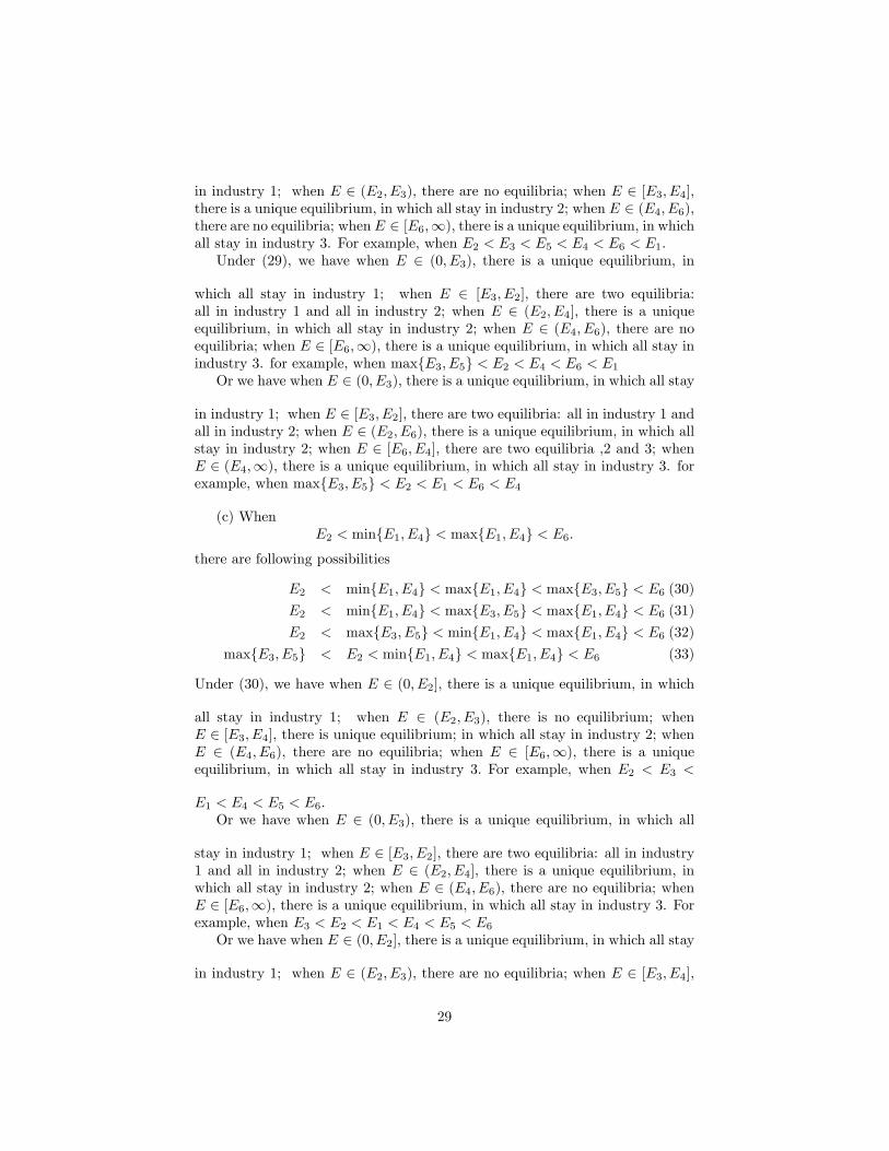
Suppose Kssi > �i for both i = 1; 2.4 There is a unique Pareto optimal

dynamic allocation as illustrated by curve BB in the following phase diagram(see Figure 1). The economy starts with a su¢ ciently small initial capital stock

4For example, it holds when

�1 = 0:1;�2 = 0:2; �3 = 0:4; �2 = 1:2; �3 = 1:44; � = 0:03; L = 100:

and� = 0:05; � = 0:05;

because then we have

E3 < E6 < �1 < �2 < Kss1 < Kss

2 < E2 < Kss3 < E4: (20)

13

K0, and all the �rms stay in industry 1, so the economy will move northeastalong the curve BB until capital reaches �1, at which point all the �rms move toindustry 2, so the economy continues to move northeast until the capital reaches�2, at which point all the �rms simultaneously shift to industry 3 and stay thereafterwards. Therefore, the economy will follow the saddle path and eventuallyconverge to the steady state SS3. In other words, it requires sequential multiplecoordination to achieve the Pareto optimality.

[Figure 1]

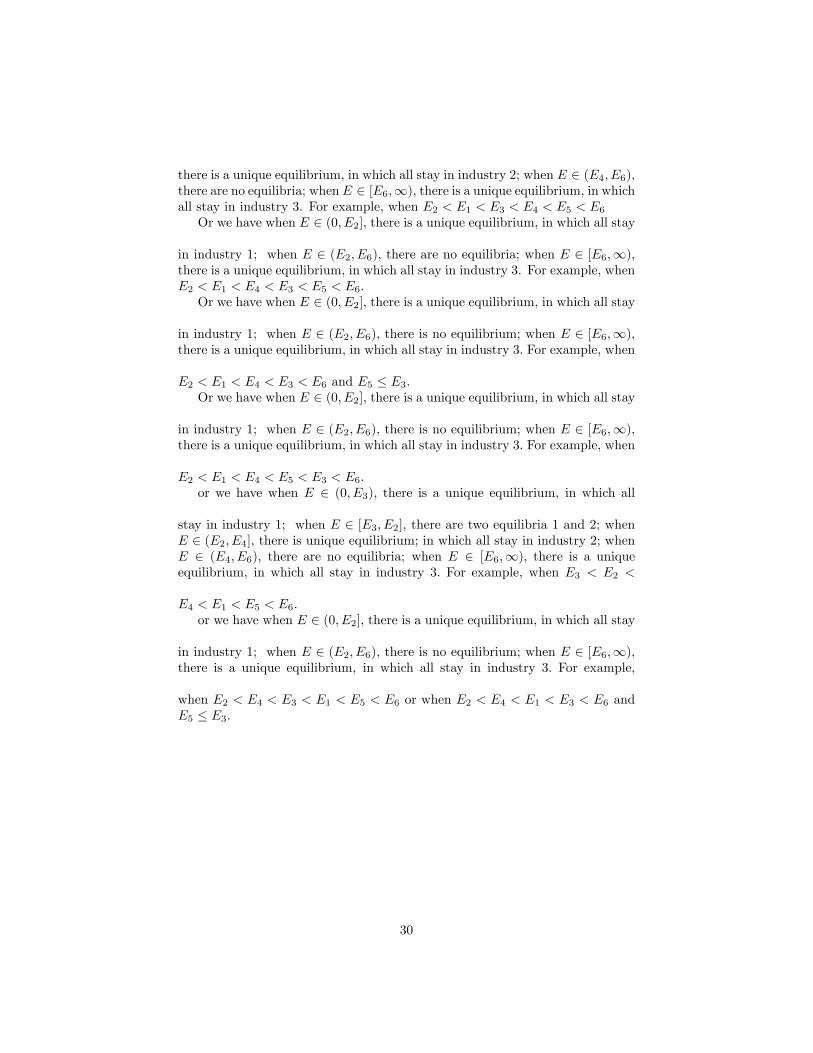
Suppose Kss1 > �1 but Kss

2 < �2. There are still several di¤erent pos-sibilities. When �2 is su¢ ciently close to Kss

2 , the Pareto optimal allocationmay follow a non-monotonic path as illustrated by curve BHB in Figure 2.The economy starts from industry 1 and then shifts to industry 2 when capitalreaches �1, after which the economy stays in industry 2 until capital reaches�2 at point H. The economy stays in industry 3 afterwards and eventuallyconverges to steady state SS3.

[Figure 2]

However, if �2 is su¢ ciently larger than Kss2 but not too large (close to

Kss3 ), then in order to approach steady state 3 by following the rule (19), the

economy would have to follow a discontinuous path as illustrated in Figure 3.The economy initially follows the lotus BH and consumption jumps from H toD precisely when capital reaches �2, the economy shifts to industry 3 afterwardsand eventually converges to steady state SS3.

[Figure 3]

Discontinuous consumption is certainly not desirable for consumers andhence cannot be Pareto optimal. When �2 is su¢ ciently larger than Kss

2 , itmay be strictly better o¤ to give up industry 3 and instead converge to steadystate SS2 with industry 2 although it is feasible to upgrade to industry 3. SeeFigure 4.

[Figure 4]

Similar reasoning also applies when Kss1 < �1, in which case the Pareto

optimal dynamic allocation may eventually converge to steady state SS1 withindustry 1 when �1 exceeds Kss

1 signi�cantly.To summarize,

Proposition 11 Suppose K(0) is su¢ ciently small. When the time discountrate � is su¢ ciently small ( Kss

i > �i for both i = 1; 2), the Pareto optimalallocation is such that industries will upgrade step by step from industry 1 toindustry 2 and then to industry 3. When � is su¢ ciently large ( Kss

1 � �1),the Pareto optimal allocation is that the industries will remain in industry 1.When � is in some middle range, the Pareto optimal allocation is such that theindustries will �rst stay in industry 1 and then upgrade to industry 2 and staythere forever.

14

4.2 Laissez-faire Market Equilibrium

Next let us examine the market equilibrium (or equilibria). At each time point,given the inherited capital stock, the equilibrium industrial choices are the sameas in the static model shown in Section 3. That is, all the �rms simultaneouslyand non-cooperatively make their industrial choices (production decision) ateach time point. The consumption and saving decisions are made after outputis produced. For simplicity, we will focus on the symmetric equilibria in whichall the �rms behave identically. To simplify the analysis, we assume �3 issu¢ ciently small (so that Corollary 8 applies) and �1 < �3 < �2 (so that Lemma9 applies).Suppose the initial capital stock is su¢ ciently small (K(0) < E3), so the

market equilibrium must start with industry 1. By revoking Corollary 8, wehave the following lemma:

Lemma 12 Industry 1 can be the industry in the long-run steady state onlyif Kss

1 2 (0; E2], industry 2 can be in the steady state only if Kss2 2 [E3; E4],

industry 3 can be in the steady state only if Kss3 2 [E6,1).

This lemma is useful in determining the steady state of the economy. Forexample, industry 1 cannot be the steady state industry if � is su¢ cientlysmall such that Kss

1 > E2. Using this logic, we can easily obtain the followingproposition after studying the associated Hamiltonian system.

Proposition 13 When � is su¢ ciently large such that Kss3 < E3, then the

only dynamic equilibrium is that industry 1 will persist forever, which is alsoPareto optimal. By contrast, when � is su¢ ciently small such that Kss

1 >E4, the economy will eventually approach steady state 3, although there mayexist multiple equilibrium transitional dynamic paths, some of which are strictlyPareto dominated.

Proof. According to Corollary 8, the market equilibrium industry must beindustry 3 whenever K(t) > E4 and must be industry 1 whenever K(t) � E3.

This proposition implies that the market equilibrium itself is Pareto optimalwhen people are su¢ ciently impatient, even though each industry exhibits Mar-shallian externality. When people are su¢ ciently patient, the market itself willsuccessfully upgrade the industry and end up with the Pareto optimal industryin the long run. The most complicated case is when � falls in the middle range,to which we now turn.Now we have E3 � Kss

3 and Kss1 � E4. In general, there could be a contin-

uum of di¤erent dynamic market equilibria. For example, consider the followingcase: Kss

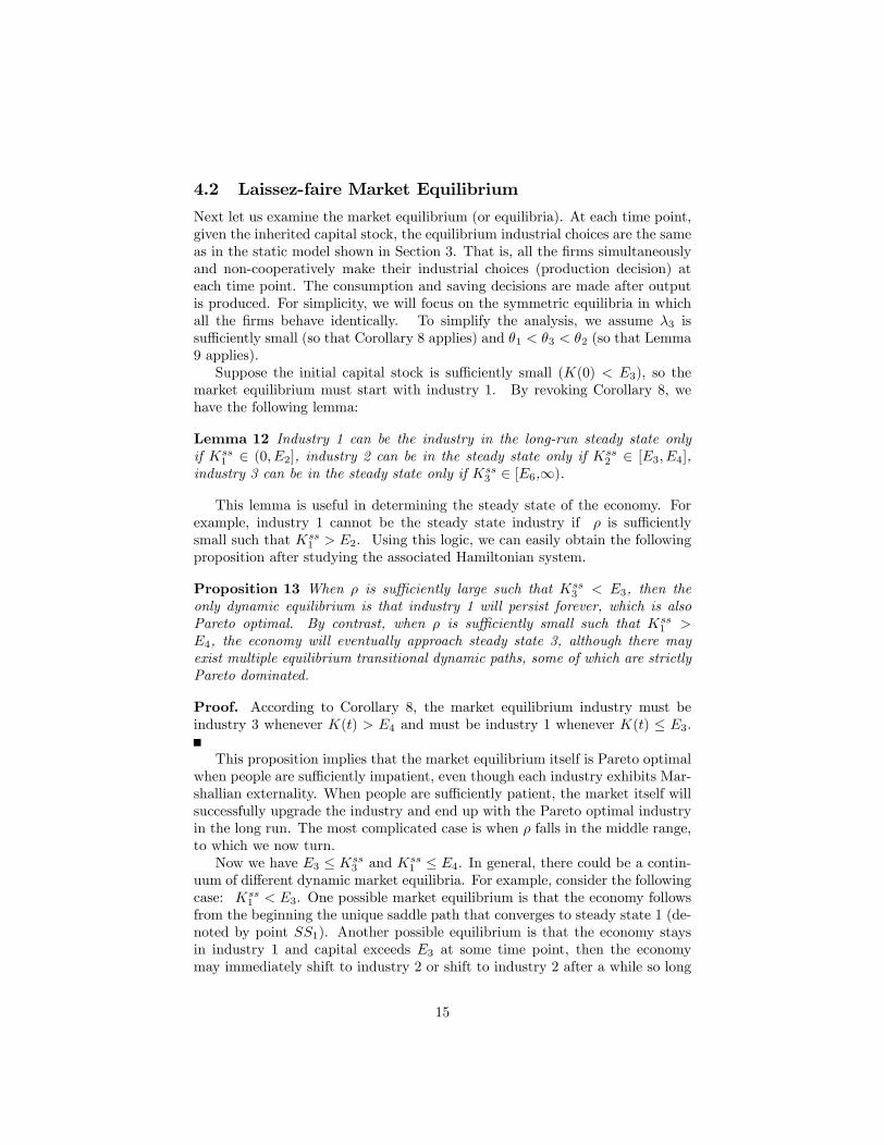
1 < E3. One possible market equilibrium is that the economy followsfrom the beginning the unique saddle path that converges to steady state 1 (de-noted by point SS1). Another possible equilibrium is that the economy staysin industry 1 and capital exceeds E3 at some time point, then the economymay immediately shift to industry 2 or shift to industry 2 after a while so long

15

as capital exceeds E3, and the economy eventually converges to steady state 2(denoted by point SS2). One possible equilibrium path is depicted by curveBHSS2 in Figure 5. Notice that the economy shifts to industry 2 at point H,which is indeterminate depending on the initial consumption (that is, the y-axisof point B). In other words, there could be in�nite such type of equilibria aslong as Kss

2 2 [E3; E4].

[FIGURE 5]

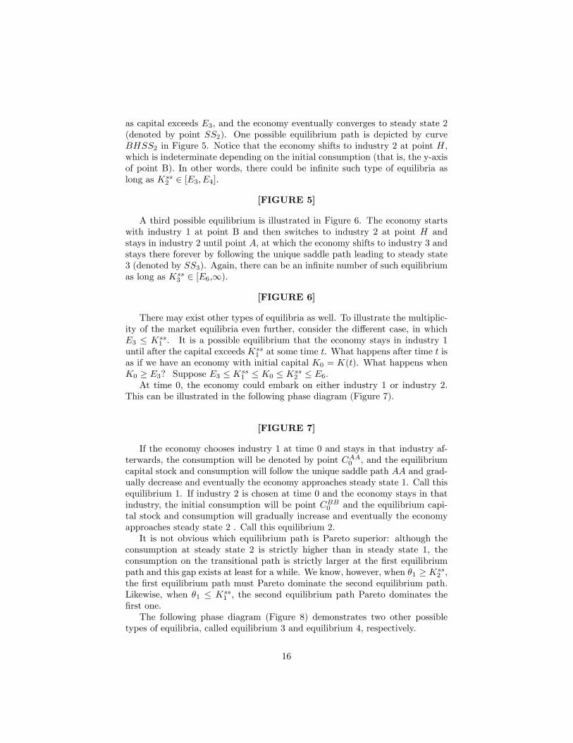
A third possible equilibrium is illustrated in Figure 6. The economy startswith industry 1 at point B and then switches to industry 2 at point H andstays in industry 2 until point A, at which the economy shifts to industry 3 andstays there forever by following the unique saddle path leading to steady state3 (denoted by SS3). Again, there can be an in�nite number of such equilibriumas long as Kss

3 2 [E6,1):

[FIGURE 6]

There may exist other types of equilibria as well. To illustrate the multiplic-ity of the market equilibria even further, consider the di¤erent case, in whichE3 � Kss

1 . It is a possible equilibrium that the economy stays in industry 1until after the capital exceeds Kss

1 at some time t. What happens after time t isas if we have an economy with initial capital K0 = K(t). What happens whenK0 � E3? Suppose E3 � Kss

1 � K0 � Kss2 � E6.

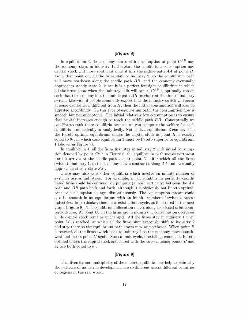
At time 0, the economy could embark on either industry 1 or industry 2.This can be illustrated in the following phase diagram (Figure 7).

[FIGURE 7]

If the economy chooses industry 1 at time 0 and stays in that industry af-terwards, the consumption will be denoted by point CAA0 , and the equilibriumcapital stock and consumption will follow the unique saddle path AA and grad-ually decrease and eventually the economy approaches steady state 1. Call thisequilibrium 1. If industry 2 is chosen at time 0 and the economy stays in thatindustry, the initial consumption will be point CBB0 and the equilibrium capi-tal stock and consumption will gradually increase and eventually the economyapproaches steady state 2 . Call this equilibrium 2.It is not obvious which equilibrium path is Pareto superior: although the

consumption at steady state 2 is strictly higher than in steady state 1, theconsumption on the transitional path is strictly larger at the �rst equilibriumpath and this gap exists at least for a while. We know, however, when �1 � Kss

2 ,the �rst equilibrium path must Pareto dominate the second equilibrium path.Likewise, when �1 � Kss

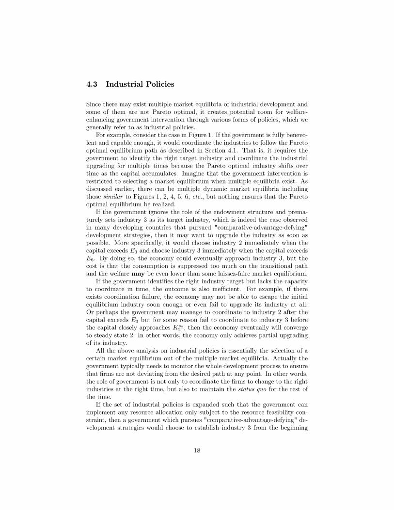
1 , the second equilibrium path Pareto dominates the�rst one.The following phase diagram (Figure 8) demonstrates two other possible

types of equilibria, called equilibrium 3 and equilibrium 4, respectively.

16

[Figure 8]

In equilibrium 3, the economy starts with consumption at point CAB0 andthe economy stays in industry 1, therefore the equilibrium consumption andcapital stock will move southeast until it hits the saddle path AA at point H.From that point on, all the �rms shift to industry 2, so the equilibrium pathwill move northeast along the saddle path BB, and the economy eventuallyapproaches steady state 2. Since it is a perfect foresight equilibrium in whichall the �rms know when the industry shift will occur, CAB0 is optimally chosensuch that the economy hits the saddle path BB precisely at the time of industryswitch. Likewise, if people commonly expect that the industry switch will occurat some capital level di¤erent from H, then the initial consumption will also beadjusted accordingly. On this type of equilibrium path, the consumption �ow issmooth but non-monotonic. The initial relatively low consumption is to ensurethat capital increases enough to reach the saddle path BB. Conceptually wecan Pareto rank these equilibria because we can compute the welfare for eachequilibrium numerically or analytically. Notice that equilibrium 3 can never bethe Pareto optimal equilibrium unless the capital stock at point H is exactlyequal to �1, in which case equilibrium 3 must be Pareto superior to equilibrium1 (shown in Figure 7).In equilibrium 4, all the �rms �rst stay in industry 2 with initial consump-

tion denoted by point CBA0 in Figure 8, the equilibrium path moves northwestuntil it arrives at the saddle path AA at point G, after which all the �rmsswitch to industry 1, so the economy moves southwest along AA and eventuallyapproaches steady state SS1.There may also exist other equilibria which involve an in�nite number of

switches across industries. For example, in an equilibrium perfectly coordi-nated �rms could be continuously jumping (almost vertically) between the AApath and BB path back and forth, although it is obviously not Pareto optimalbecause consumption changes discontinuously. The consumption stream couldalso be smooth in an equilibrium with an in�nite number of switches acrossindustries. In particular, there may exist a limit cycle, as illustrated in the nextgraph (Figure 9). The equilibrium allocation moves along the closed orbit coun-terclockwise. At point G, all the �rms are in industry 1, consumption decreaseswhile capital stock remains unchanged. All the �rms stay in industry 1 untilpoint M is reached, at which all the �rms simultaneously shift to industry 2and stay there so the equilibrium path starts moving northeast. When point Bis reached, all the �rms switch back to industry 1 so the economy moves south-west and meets point G again. Such a limit cycle, if existing, cannot be Paretooptimal unless the capital stock associated with the two switching points B andM are both equal to �1.

[Figure 9]

The diversity and multiplicity of the market equilibria may help explain whythe patterns of industrial development are so di¤erent across di¤erent countriesor regions in the real world.

17

4.3 Industrial Policies

Since there may exist multiple market equilibria of industrial development andsome of them are not Pareto optimal, it creates potential room for welfare-enhancing government intervention through various forms of policies, which wegenerally refer to as industrial policies.For example, consider the case in Figure 1. If the government is fully benevo-

lent and capable enough, it would coordinate the industries to follow the Paretooptimal equilibrium path as described in Section 4.1. That is, it requires thegovernment to identify the right target industry and coordinate the industrialupgrading for multiple times because the Pareto optimal industry shifts overtime as the capital accumulates. Imagine that the government intervention isrestricted to selecting a market equilibrium when multiple equilibria exist. Asdiscussed earlier, there can be multiple dynamic market equilibria includingthose similar to Figures 1, 2, 4, 5, 6, etc., but nothing ensures that the Paretooptimal equilibrium be realized.If the government ignores the role of the endowment structure and prema-

turely sets industry 3 as its target industry, which is indeed the case observedin many developing countries that pursued "comparative-advantage-defying"development strategies, then it may want to upgrade the industry as soon aspossible. More speci�cally, it would choose industry 2 immediately when thecapital exceeds E3 and choose industry 3 immediately when the capital exceedsE6. By doing so, the economy could eventually approach industry 3, but thecost is that the consumption is suppressed too much on the transitional pathand the welfare may be even lower than some laissez-faire market equilibrium.If the government identi�es the right industry target but lacks the capacity

to coordinate in time, the outcome is also ine¢ cient. For example, if thereexists coordination failure, the economy may not be able to escape the initialequilibrium industry soon enough or even fail to upgrade its industry at all.Or perhaps the government may manage to coordinate to industry 2 after thecapital exceeds E3 but for some reason fail to coordinate to industry 3 beforethe capital closely approaches Kss

2 , then the economy eventually will convergeto steady state 2. In other words, the economy only achieves partial upgradingof its industry.All the above analysis on industrial policies is essentially the selection of a

certain market equilibrium out of the multiple market equilibria. Actually thegovernment typically needs to monitor the whole development process to ensurethat �rms are not deviating from the desired path at any point. In other words,the role of government is not only to coordinate the �rms to change to the rightindustries at the right time, but also to maintain the status quo for the rest ofthe time.If the set of industrial policies is expanded such that the government can

implement any resource allocation only subject to the resource feasibility con-straint, then a government which pursues "comparative-advantage-defying" de-velopment strategies would choose to establish industry 3 from the beginning

18

and it can also eventually achieve industry 3, which can never be achieved by themarket itself. Of course, it is not Pareto optimal because the total consumptionis depressed too much.In the pertinent literature, to tackle the multiplicity of market equilibria, it is

often assumed that there exists an ad hoc frictional adjustment process, so thatwhether the industrial upgrading occurs depends on whether "expectation" candominate "history", which in turns depends on the magnitude of the discountrate and the parameters of the adjustment process (see, for example, Krugman,1991). If the discount rate is su¢ ciently large and/or the adjustment processis su¢ ciently di¢ cult, then "history" dominates and therefore there is a uniqueequilibrium, in which industrial upgrading (or industrialization) cannot occur,otherwise "expectation" dominates and there are multiple equilibria, some ofwhich have industrial upgrading. Our previous proposition already partly char-acterizes how the market equilibrium is a¤ected by the time discount rate. Now,to simplify the analysis, suppose that economy starts with initial capital smallerthan E3 and has the strongest path dependence (by revoking Corollary 8) in thesense that the equilibrium remains to be that "all the industries are in industry1" whenever K(t) 2 (0; E2]. When K(t) exceeds E2, all the �rms could eithersuddenly shift to industry 2 or all move to industry 3, depending on people�sexpectation; and the industries will stay in industry 3 when K(t) > E4.In particular, if we resort to the argument that the �rst mover would unilat-

erally deviate from industry 1 to industry 3 when K(t) just crosses E2, whichcan be veri�ed, then it implies

i�(t) =

�1; when K(t) � E23; when E2 < K(t)

: (21)

If, however, we assume that there exists some su¢ ciently small cost of industrialupgrading and the cost is larger when directly shifting from 1 to 3 than thatwhen shifting from 1 to 2, holding other things unchanged, then the marketequilibrium industry is

i�(t) =

8<: 1; when K(t) � E22; when E2 < K(t) � E43; when K(t) > E4

: (22)

To make the analysis concrete, consider the following parametric example:

�1 = 0:1;�2 = 0:2; �3 = 0:4; �2 = 1:2; �3 = 1:44; � = 0:03; L = 100; � = 0:05; � = 0:05;

then we have

E3 < E6 < �1 < �2 < Kss1 < Kss

2 <

��1A(L)

�

� 11��1

L < E2 < Kss3 < E4;

then under rule (21) or rule (22), there exists a unique market equilibrium, inwhich the �rms always stay in industry 1 and the economy eventually converges

19

to steady state 1.5 By contrast, the Pareto optimal equilibrium for this nu-merical example is exactly given by Figure 1 and the economy will eventuallyconverge to steady state 3. This comparison implies that this "constrained" mar-ket equilibrium is not Pareto optimal, therefore, the government may improvethe welfare by appropriately "relaxing" the "path dependence" constraint, andalleviating all the constraints once and for all is not su¢ cient to ensure that thePareto optimal equilibrium be realized because there are many possible marketequilibria.So far we have not been explicit about the concrete policy tools that govern-

ment can employ to implement its industrial policy. Traditional policy variablesinclude the provision of various forms of subsidies, such as tax rebate/holidays,investment credit, export subsidy, etc., for those investors/�rms that follow therecommendation of the government. Policy variables also include imposing pun-ishment, through tax for example, on those investors/�rms that do not followthe recommendation of the government. All these policy tools are applicablehere. It is worth mentioning that, in our model economy, it is often the casethat the Pareto optimal allocation can be achieved by the market itself, althoughnot ensured because there are multiple equilibria. Under that circumstance, thebest the government can do is just to help reduce the coordination cost amongthe �rms because each �rm/investor has su¢ ciently strong incentive to achievethe Pareto optimal equilibrium and there is no con�ict of interest among thoseidentical investors/�rms. When the Pareto optimal allocation can never be im-plemented by the market itself because, for example, there exists coordinationfailure or su¢ ciently large cost associated with the e¢ ciency-enhancing collec-tive action as we have just discussed, then the government should rectify therelevant market failure with carrot and stick.Most importantly, we want to emphasize that the crucial prerequisite for

successful industrial policy is that the government identi�es the "right" indus-try target in time, that is, the industry which is most consistent with the capitalendowment of the economy. The existence of Marshallian externality itself is in-su¢ cient to justify government support for that industry. Moreover, the "right"industry target may endogenously shift over time as the economy develops,therefore successful industrial policy may require sequential and timely "push"instead of "once-and-for-all" intervention, as typically examined in the exist-ing literature. To illustrate the importance of "right identi�cation", we showthat when the government identi�es the wrong industrial target and "push" itaccordingly, the economy may be even worse o¤ than the laissez-faire market

5This is the unique equilibrium under rule (21) because E2 �h�1A(L)

�

i 11��1 L, sinceh

�1A(L)�

i 11��1 L is the largest possible value for capital when the initial capital is su¢ ciently

small. If E2 <h�1A(L)

�

i 11��1 L, there may exist a second equilibrium, in which the economy

stays in industry 1 until the capital reaches E2, after which the economy swtiches to industry3 and moves along the saddle path leading to steady state 3. If rule (22) is adopted, no matter

whether E2 �h�1A(L)

�

i 11��1 L holds or not, there will be a unique equlibrium, in which the

�rms always stay in industry 1 and the economy eventually converges to steady state 1.

20

equilibrium even though the target industry does exhibit Marshallian external-ity.

5 Further Discussion

In this section, we show that our theoretical results are robust when certainassumptions in the model setting are changed.

5.1 Sequential Entrance

The market equilibrium at each time point in our previous analysis is the staticNash equilibrium. What would be the subgame Nash equilibrium if �rms areallowed to move sequentially? Suppose E�� � E� < E: The �rst �rm wants tomove from industry 1 to industry 2 holding other �rms staying in industry 1.Now given that the �rst mover has moved, would there be a second mover atthe same level of E? If he stays, he earns

(1� �1)A(L� 1)�E � k02L� 1

��1;

where k02 is uniquely determined by (7). If he moves to industry 2, he earns

(1� �2)�A(2)k"�22 ;

where k"2 is uniquely determined by

�1A(L� 2)�E � 2k"2L� 2

��1�1= �2�A(2)k

"�2�12 :

Using the argument with equation (2) in the proof of Proposition 2, we havek"2 > k02, which in turn implies

(1� �2)�A(2)k"�22 > (1� �2)�A(1)k0�22

> (1� �1)A(L)�E

L

��1> (1� �1)A(L� 1)

�E � k02L� 1

��1;

where the second inequality is because E > E� as we have shown and thelast inequality holds when k02 > E

L , which holds if and only if�1A(L�1)�2�A(1)

<�EL

��2��1 . Consequently, this second agent �nds it strictly pro�table to alsomove to industry 2 when �1A(L�1)

�2�A(1)<�E�

L

��2��1, which is equivalent to

24 (1��1)A(L)(1��2)

�1A(L�1)�2

35(1��2)=�22641�

24 (1��1)A(L)(1��2)

�1A(L�1)�2

351=�2 =L375�1�1

> (L� 1)�1�1 L1��1 :

21

The above inequality is true if L is su¢ ciently large, which we will assume truethroughout the paper.Then as implied by Lemma 1, the rest of the �rms in industry 1 will enter

industry 2 one by one until there is only one �rm remaining in industry 1. Thelast �rm has incentives to move to industry 2 if and only if E > E��, whichindeed holds. Consequently, when E�� � E� < E, there is a unique subgameNash equilibrium in which all the �rms will be staying in industry 2. So theequilibrium outcome is identical to that in the static Nash equilibrium.

5.2 Di¤erent A(n) Function

People may wonder whether our results depend on the fact that the externalitybecomes increasingly stronger when A(n) takes the form of an exponential func-tion, as we assume in our previous analysis. To address this question, supposenothing changes except that now the function A(n) becomes

A(n) = A0n�, where � 2 (0; 1);

so that the marginal increase in the "magnitude" of Marshallian externality isdiminishing when more �rms enter the same industry. We �rst characterize E�.The function (9) becomes

�1(L� 1)�+1��1E��1=�2�1"1�

�(1� �1)L���1�(1� �2)

�1=�2E�

�1�2�1#�1�1

= �2�1=�2

�(1� �1)L���1(1� �2)

�(�2�1)=�2: (23)

It implies

@E� (�; L; �1; �2; �)

@�< 0; lim

�!1E� (�; L; �1; �2; �) = 0:

Also, suppose � � �1, then

@E� (�; L; �1; �2; �)

@L> 0; lim

L!1E� (�; L; �1; �2; �) =1:

and the intuition is that, the larger the population, the cheaper the labor andalso the stronger the Marshallian externality in the current industry, hence theweaker the incentive to deviate away from the less capital-intensive industry.And

@E� (�; L; �1; �2; �)

@�> 0.

Next we characterize E��. (14) becomes

�1

�(1� �2)L���2(1� �1)

��1�1�1

= �2�2� 1

�1 (L� 1)�+1��2E���2�1�1"1�

�(1� �2)L���2�(1� �1)

� 1�1

E���2�1�1#�2�1

;

22

from which we conclude: [1] @E��(�;L;�1;�2;�)

@� > 0 and lim�!1

E� (�; L; �1; �2; �) =

1, when �1 � 12 ; [2] suppose � � �2, then

@E��(�;L;�1;�2;�)@L < 0 and lim

L!1E� (�; L; �1; �2; �) =

0; [3]@E��(�;L;�1;�2;�)

@� < 0. We can see that the main properties of functionsE� (�; L; �1; �2; �) and E�� (�; L; �1; �2; �) are almost the same as in the pre-vious analysis. This implies that all the qualitative features in the previousanalysis will remain intact.

6 Conclusion

In this paper we develop a growth model with multiple industries to study howindustries evolve as capital accumulates endogenously when each industry ex-hibits Marshallian externality (increasing returns to scale). We show that, in thelong run, the laissez-faire market equilibrium is Pareto optimal when the timediscount rate is su¢ ciently small or su¢ ciently large. When the time discountrate is moderate, there exists a very rich set of multiple dynamic market equi-libria, some of which are Pareto dominated. This may help explain why diversepatterns of industrial development are observed in the real world. To ensurethe economy achieve Pareto e¢ ciency, it would require the government to �rstidentify the industry target consistent with the endowment structure and thento coordinate in a timely manner, possibly for multiple times. However, indus-trial policies may make people worse o¤ than in the market equilibrium if thegovernment picks an industry which deviates too far away from the comparativeadvantage of the economy even if the industry exhibits Marshallian externality.This may help explain why industrial policies succeeded in some countries butfailed in others and why sometimes industrial upgrading may take place evenwithout government support.Di¤erent from the literature, we highlight that the mere existence of Mar-

shallian externality in an industry is insu¢ cient to justify government supportfor that industry. Instead, a crucial prerequisite for successful industrial poli-cies is to �rst identify the "right" industry target in time, that is, the industrywhich is most consistent with the capital endowment of the economy. Moreover,we show that the "right" industry target may endogenously shift over time asthe economy develops, therefore successful industrial policy may require sequen-tial and timely "pushes" instead of "once-and-for-all" intervention, as typicallyargued in the existing literature. To illustrate the importance of "right iden-ti�cation", we show that when the government identi�es the wrong industrialtarget and "pushes" it accordingly, the economy may be even worse o¤ than thelaissez-faire market equilibrium even though the target industry does exhibitMarshallian externality.For the sake of analytical simplicity, just like the standard models in the

literature, our model also assumes away uncertainty associated with the iden-ti�cation of the right "industrial target". We also ignore the case where thereare multiple industries with similar capital intensities but insu¢ cient numberof investors (either because of the credit constraint or the scarcity of quali�ed

23

entrepreneurs). Thirdly, industry-speci�c productivity growth is not incorpo-rated into our analyses. It would be interesting to explore those and many otherissues in the future.

24

References

[1] Balassa, Bela,1971. The Structure of Protection in Developing Countries.Baltimore, MD, Johns Hopkins University Press .

[2] Canda, Vandana. 2006. Technology, Adaptation, and Exports: How SomeDeveloping Countries Got It Right. World Bank

[3] Chang, H.-J., 2003. Kicking Away the Ladder: Development Strategy inHistorical Perspective, London, Anthem Press.

[4] Harrison, Ann and Andres Rodriguez-Clare. 2009. Trade, Foreign Invest-ment, and Industrial Policies for Developing Countries. Manuscript pre-pared for Handbook of Development Economics. edited by Dani Rodrik

[5] Ju, Jiandong, Justin Yifu Lin and Yong Wang. 2010, "Endowment Struc-ture, Industrial Dynamics and Economic Growth", working paper

[6] Krugman, Paul. 1987. "The Narrow Moving Band, The Dutch Disease, andThe Competitive Consequences of Mrs. Thatcher". Journal of DevelopmentEconomics 27: 41-55

[7] 1991. "History Versus Expectations", Quarterly Journal of Economics106(2): 651-667

[8] Lin, Justin Yifu. 2009. Marshall Lectures: Economic Development andTransition: Thought, Strategy, and Viability. London: Cambridge Univer-sity Press

[9] � � and Celestin Monge, 2010. Growth identi�cation and facilitation :the role of the state in the dynamics of structural change, Policy ResearchWorking Paper #5313, World Bank

[10] Matsuyama, Kiminori. 1991. Increasing Returns, Industrialization, and In-determinacy of Equilibrium. Quarterly Journal of Economics 106(2): 617-650

[11] Murphy, Kevin M.; Andrei Shleifer and Robert W. Vishny, 1989. Industri-alization and Big Push. Journal of Political Economy, 97(5): 1003-1026

[12] Mussa, Michael. 1978. "Dynamic Adjustment in the Heckscher-Ohlin-Samuelson Model", Journal of Political Economy, 86(5): 775-791

[13] Ohashi, Hiroshi, 2005. �Learning by Doing, Export Subsidies, and IndustryGrowth: Japanese Steel in the 1950s and 1960s,�Journal of InternationalEconomics, Vol. 66(2): 297�323

[14] Pack, Howard, and Kamal Saggi. 2006. �Is There a Case for IndustrialPolicy? A Critical Survey,� The World Bank Research Observer, 21(2):267�297.

25

[15] Panagariya, Arvind. 1986. "Increasing Returns, Dynamic Stability, andInternational Trade", Journal of International Economics 40: 43-63

[16] Rodriguez-Clare, Andres, 2007. Clusters and Comparative Advantage: Im-plications for Industrial Policy, Journal of Development Economics 82: 43-57

[17] Rodrik, D., 1996. Coordination Failures and Government Policy: A Modelwith Applications to East Asia and Eatern Europe, Journal of InternationalEconomics 40: 1-22

[18] � � , 2008. Normalizing Industrial Policies, Washington, DC. World BankPres

[19] Wade, Robert.1990. Governing the Market: Economic Theory and the Roleof Government in East Asian Industrialization. Princeton University Press

26

Appendix 1:

When E6 > E2, we could have

E2 < E6 < minfE1; E4g:

orE2 < minfE1; E4g < E6 < maxfE1; E4g:

orE2 < minfE1; E4g < maxfE1; E4g < E6:

More speci�cally,(a) when

E2 < E6 < minfE1; E4g;

there are following possibilities

maxfE3; E5g < E2 < E6 < minfE1; E4g (24)

minfE3; E5g < E2 < maxfE3; E5g < E6 < minfE1; E4g (25)

E2 < minfE3; E5g < maxfE3; E5g < E6 < minfE1; E4g (26)

Under (24), we have when E 2 (0; E3); there is a unique equilibrium, in which all

stay in industry 1; when E 2 [E3; E2]; there are two equilibria: all in industry 1and all in industry 2; when E 2 (E2; E6), there is a unique equilibrium, in whichall stay in industry 2; when E 2 [E6; E4], there are two equilibria: all in industry2 and all in industry 3; when E 2 (E4;1); there is a unique equilibrium, inwhich all stay in industry 3.Under (25), we have when E 2 (0; E2); there is a unique equilibrium, in

which all stay in industry 1; when E 2 [E2; E6], there is a unique equilibrium,in which all stay in industry 2; when E 2 (E6; E4], there are two equilibria:all in industry 2 and all in industry 3; when E 2 (E4;1); there is a uniqueequilibrium, in which all stay in industry 3.Under (26), we have when E 2 (0; E2]; there is a unique equilibrium, in

which all stay in industry 1; when E 2 (E2; E3), there is no equilibrium; whenE 2 (E3; E6), there is unique equilibrium; in which all stay in industry 2; whenE 2 [E6; E4], there are two equilibria: all in industry 2 and all in industry 3;when E 2 (E4;1); there is a unique equilibrium, in which all stay in industry3.

(b)WhenE2 < minfE1; E4g < E6 < maxfE1; E4g:

27

there are following possibilities

E2 < minfE1; E4g < maxfE3; E5g < E6 < maxfE1; E4g (27)E2 < maxfE3; E5g < minfE1; E4g < E6 < maxfE1; E4g (28)

maxfE3; E5g < E2 < minfE1; E4g < E6 < maxfE1; E4g (29)

Under (27), we have when E 2 (0; E2]; there is a unique equilibrium, in which

all stay in industry 1; when E 2 (E2; E3); there is no equilibrium; when E 2[E3; E6), there is unique equilibrium: industry 2; when E 2 (E6; E4], there aretwo equilibria: all in industry 2 and all in industry 3; when E 2 (E4;1); thereis a unique equilibrium, in which all stay in industry 3.Or we have when E 2 (0; E3); there is a unique equilibrium, in which all stay

in industry 1; when E 2 [E3; E2]; there are two equilibria: all in industry 1 andall in industry 2; when E 2 [E2; E6], there is a unique equilibrium, in which allstay in industry 2; when E 2 (E6; E4], there are two equilibria: all in industry2 and all in industry 3; when E 2 (E4;1); there is a unique equilibrium, inwhich all stay in industry 3.Or we have when E 2 (0; E2]; there is a unique equilibrium, in which all stay

in industry 1; when E 2 (E2; E6), there is no equilibrium, when E 2 [E6;1);there is a unique equilibrium, in which all stay in industry 3. For example, whenE5 < E2 < E4 < E3 < E6 < E1:

Under (28), we have when E 2 (0; E3); there is a unique equilibrium, in

which all stay in industry 1; when E 2 [E3; E2]; there are two equilibria:all in industry 1 and all in industry 2; when E 2 [E2; E6], there is a uniqueequilibrium, in which all stay in industry 2; when E 2 (E6; E4], there are twoequilibria: all in industry 2 and all in industry 3; when E 2 (E4;1); there is aunique equilibrium, in which all stay in industry 3.Or we have when E 2 (0; E2]; there is a unique equilibrium, in which all stay

in industry 1; when E 2 (E2; E3); there is no equilibrium; when E 2 [E3; E6),there is unique equilibrium: industry 2; when E 2 (E6; E4], there are twoequilibria: all in industry 2 and all in industry 3; when E 2 (E4;1); there is aunique equilibrium, in which all stay in industry 3.Or we have when E 2 (0; E3); there is a unique equilibrium, in which all

stay in industry 1; when E 2 [E3; E2]; there are two equilibria: all in industry1 and all in industry 2; when E 2 [E2; E4], there is a unique equilibrium, inwhich all stay in industry 2; when E 2 (E4; E6), there are no equilibria; whenE 2 [E6;1); there is a unique equilibrium, in which all stay in industry 3. Forexample, when E3 < E2 < E5 < E4 < E6 < E1Or we have when E 2 (0; E2]; there is a unique equilibrium, in which all stay

28

in industry 1; when E 2 (E2; E3); there are no equilibria; when E 2 [E3; E4],there is a unique equilibrium, in which all stay in industry 2; when E 2 (E4; E6),there are no equilibria; when E 2 [E6;1); there is a unique equilibrium, in whichall stay in industry 3. For example, when E2 < E3 < E5 < E4 < E6 < E1:Under (29), we have when E 2 (0; E3); there is a unique equilibrium, in

which all stay in industry 1; when E 2 [E3; E2]; there are two equilibria:all in industry 1 and all in industry 2; when E 2 (E2; E4], there is a uniqueequilibrium, in which all stay in industry 2; when E 2 (E4; E6), there are noequilibria; when E 2 [E6;1); there is a unique equilibrium, in which all stay inindustry 3. for example, when maxfE3; E5g < E2 < E4 < E6 < E1Or we have when E 2 (0; E3); there is a unique equilibrium, in which all stay

in industry 1; when E 2 [E3; E2]; there are two equilibria: all in industry 1 andall in industry 2; when E 2 (E2; E6), there is a unique equilibrium, in which allstay in industry 2; when E 2 [E6; E4], there are two equilibria ,2 and 3; whenE 2 (E4;1); there is a unique equilibrium, in which all stay in industry 3. forexample, when maxfE3; E5g < E2 < E1 < E6 < E4

(c) WhenE2 < minfE1; E4g < maxfE1; E4g < E6:

there are following possibilities

E2 < minfE1; E4g < maxfE1; E4g < maxfE3; E5g < E6 (30)

E2 < minfE1; E4g < maxfE3; E5g < maxfE1; E4g < E6 (31)

E2 < maxfE3; E5g < minfE1; E4g < maxfE1; E4g < E6 (32)

maxfE3; E5g < E2 < minfE1; E4g < maxfE1; E4g < E6 (33)

Under (30), we have when E 2 (0; E2]; there is a unique equilibrium, in which

all stay in industry 1; when E 2 (E2; E3), there is no equilibrium; whenE 2 [E3; E4], there is unique equilibrium; in which all stay in industry 2; whenE 2 (E4; E6), there are no equilibria; when E 2 [E6;1); there is a uniqueequilibrium, in which all stay in industry 3. For example, when E2 < E3 <

E1 < E4 < E5 < E6:Or we have when E 2 (0; E3); there is a unique equilibrium, in which all

stay in industry 1; when E 2 [E3; E2]; there are two equilibria: all in industry1 and all in industry 2; when E 2 (E2; E4], there is a unique equilibrium, inwhich all stay in industry 2; when E 2 (E4; E6), there are no equilibria; whenE 2 [E6;1); there is a unique equilibrium, in which all stay in industry 3. Forexample, when E3 < E2 < E1 < E4 < E5 < E6Or we have when E 2 (0; E2]; there is a unique equilibrium, in which all stay

in industry 1; when E 2 (E2; E3); there are no equilibria; when E 2 [E3; E4],

29

there is a unique equilibrium, in which all stay in industry 2; when E 2 (E4; E6),there are no equilibria; when E 2 [E6;1); there is a unique equilibrium, in whichall stay in industry 3. For example, when E2 < E1 < E3 < E4 < E5 < E6Or we have when E 2 (0; E2]; there is a unique equilibrium, in which all stay

in industry 1; when E 2 (E2; E6); there are no equilibria; when E 2 [E6;1);there is a unique equilibrium, in which all stay in industry 3. For example, whenE2 < E1 < E4 < E3 < E5 < E6:Or we have when E 2 (0; E2]; there is a unique equilibrium, in which all stay

in industry 1; when E 2 (E2; E6), there is no equilibrium; when E 2 [E6;1);there is a unique equilibrium, in which all stay in industry 3. For example, when

E2 < E1 < E4 < E3 < E6 and E5 � E3:Or we have when E 2 (0; E2]; there is a unique equilibrium, in which all stay

in industry 1; when E 2 (E2; E6), there is no equilibrium; when E 2 [E6;1);there is a unique equilibrium, in which all stay in industry 3. For example, when

E2 < E1 < E4 < E5 < E3 < E6:or we have when E 2 (0; E3); there is a unique equilibrium, in which all

stay in industry 1; when E 2 [E3; E2], there are two equilibria 1 and 2; whenE 2 (E2; E4], there is unique equilibrium; in which all stay in industry 2; whenE 2 (E4; E6), there are no equilibria; when E 2 [E6;1); there is a uniqueequilibrium, in which all stay in industry 3. For example, when E3 < E2 <

E4 < E1 < E5 < E6:or we have when E 2 (0; E2]; there is a unique equilibrium, in which all stay

in industry 1; when E 2 (E2; E6), there is no equilibrium; when E 2 [E6;1);there is a unique equilibrium, in which all stay in industry 3. For example,

when E2 < E4 < E3 < E1 < E5 < E6 or when E2 < E4 < E1 < E3 < E6 andE5 � E3:

30

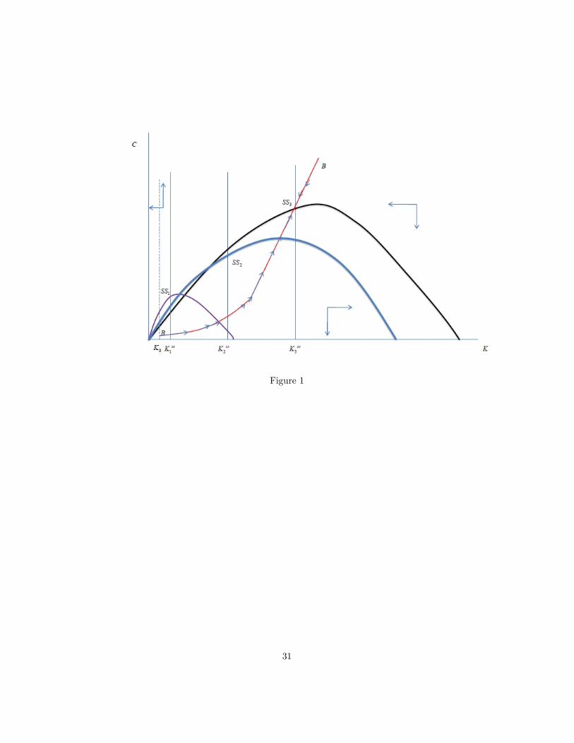
Figure 1

31

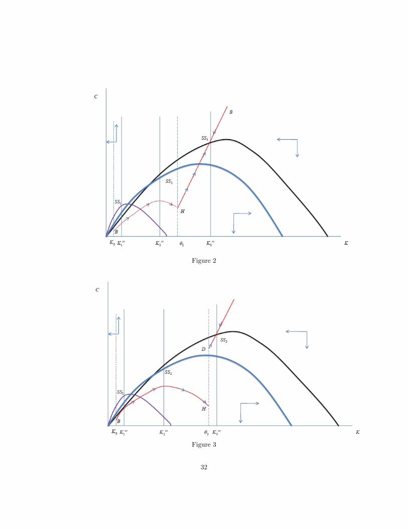
Figure 2

Figure 3

32

Figure 4

33

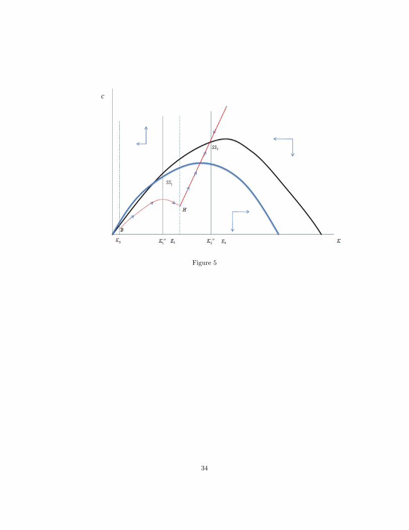
Figure 5

34

Figure 6

Figure 7

35

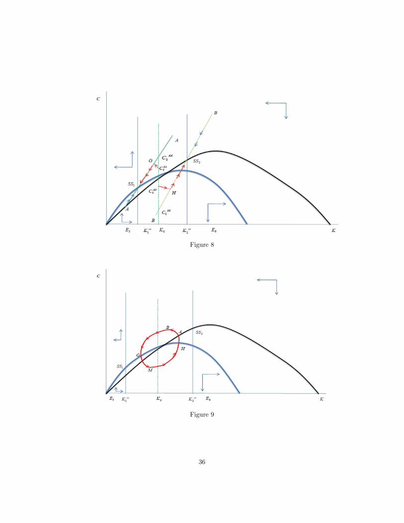
Figure 8

Figure 9

36