Mars Orbiter Laser Altimeter:Receiver Model and Performance Analysis

James B. AbshireXiaoli Sun

Robert S. Afzal

NASA Goddard Space Flight CenterLaser Remote Sensing Branch, Code 924

Greenbelt, Maryland 20771

(301) 614-6717james.abshire@gsfc.nasa.gov

August, 1999

Abstract

The measurement approach, receiver design, data conversion andcalibration of the Mars Orbital Laser Altimeter (MOLA) are described.The MOLA measurements include the range to the surface, which isdetermined by the laser pulse time-of-flight, the surface slope deter-mined by the received laser pulse width, and the surface reflectivitydetermined by the ratio of the transmitted and the received laser pulseenergies. The instrument performance is analyzed for these measure-ments.

1

1 Introduction

The Mars Orbiter Laser Altimeter (MOLA) [1, 2, 3] is one of the four in-struments on board NASA’s Mars Global Surveyor (MGS) spacecraft [4].Figure 1 shows a sketch of MGS spacecraft and MOLA instrument. MOLAmeasures the distance from the MGS spacecraft to the Mars surface by mea-suring the time-of-flight of its laser pulses. The topographic height of theplanet’s surface at the laser footprint spot is then determined through thegeometry of the planet radius, the spacecraft orbit altitude, and the pointingangle of the instrument. A simplified measurement geometry is shown inFigure 2 and the specifications for MOLA are given in Table 1..

The accuracy of the surface height determination is governed by uncer-tainties in the time of flight measurement, the spacecraft position, and thepointing angle of the laser beam. The range from MGS spacecraft to thetarget is related to the laser pulse time-of-flight by

Rm =c Topt

2(1)

with c = 299792458m/s the vacuum speed of light [5]. Here we have neglectedthe effect of atmosphere path delay, which is only a few centimeters on Marsdue to the low (4-6mbar) surface pressure. The topography or the surfaceheight at the laser footprint can be written as

hs =[R2MGS +R2

m − 2RmRMGScos(φ)]1/2−Rref (2)

where RMGS is the radius of the MGS spacecraft, φ is the pointing anglewith respect to nadir, and Rref is the reference surface of the planet which isoften taken to be the geoid.

For measurements from space, a small laser beam pointing uncertaintycan cause a sizable difference between the actual and the predicted laserfootprint location on the ground. The resultant ranging error due to pointinguncertainty is given as [6, 7]

σφ ≈ Rm

[tan2(φ+ θ‖)V ar(∆φ‖) +

tan2θ⊥cos2θ‖cos

2φ

cos2(φ+ θ‖)V ar(∆φ⊥)

]1/2

(3)

where θ‖ and θ⊥ are the effective surface slopes parallel and perpendicular tothe plane of the expected laser beam and nadir axes, and ∆φ‖ and ∆φ⊥ arethe pointing uncertainties in the two directions.

2

The MGS spacecraft pointing knowledge is less than 1 mrad after postnavigation signal processing [8]. This gives a range uncertainty of 7 metersfor a 400km average range, nadir pointing, 1 degree surface slope, and thepointing error in the same direction as the surface slope. Since the pointingerror is a slowly varying random variable, it usually spatially displaces thefootprint location in the ground track and has little effect on the measure-ments of local topography features.

In addition to the laser pulse time-of-flight, MOLA also measures thetransmitted and the echo laser pulse energies and the echo pulse width atthe threshold crossings. The full echo pulse energy and the rms pulse widthcan be solved as long as the pulse shape is known.

The pulse energies can be used to determine the surface reflectivity byusing laser altimeter link equation

Er = Etrτr ·Ar

R2m

·rs

π· τ 2a (4)

where

Er: received signal pulse energy (Joule),Etr: transmitted laser pulse energy (Joule),τr receiver optics transmission,Ar: receiver telescope entrance aperture area (m2),rs: target surface diffusive reflectivity,τa: Mars atmosphere transmission, one way.

The echo pulse width can be used to estimate the surface slope and rough-ness within the laser footprint. The surface slope of Mars is usually muchlarger than the spacecraft off-nadir pointing angle. If roughness is neglected,the rms pulse width of the echo laser pulse is related to the surface slope as[6]

< σ2r >= (σ2

x + σ2f ) +

4R2m

c2

[tan4(γ) + tan2(γ)tan2(θ)

], (5)

where σx is the transmitted laser rms pulse width, σf is the rms receiverimpulse response, and γ is the rms laser beam divergence angle (half angleat the 1/

√e intensity point). The first term in the bracket of Eq. (5) accounts

for the laser beam curvature effect and can often be neglected since usuallyγ << θ.

3

The laser pulse time-of-flight, the echo laser pulse energy and rms pulsewidth, can be determined from the MOLA measurements by using the proce-dures outlined in the rest of this paper under the following assumptions: thetransmitted and the received pulse shapes are Gaussian and the instrumentreceiver is at its nominal operating temperature. On flight measurement dataindicate that there have been no significant MOLA receiver changes since itspre-launch calibration.

2 Laser Transmitter

The MOLA laser transmitter is a diode-laser pumped, Q-switched, Cr:Nd:YAGslab laser. The laser design details and a performance model is given in [9].The nominal transmitted pulse energy is 45 mJ and the pulsewidth is 8 nsfull width at half maximum (FWHM). The laser beam full divergence anglewas measured to be 0.42 mrad at the 90% encircled energy in the far field.Assuming Gaussian beam profile, the corresponding rms beam divergenceangle was 0.093 mrad.

A small amount of the transmitted laser light is collected and coupled intothe start pulse photodetector via a multimode optical fiber. The transmittedpulse energy is measured by the start pulse energy counter, which consistsof a charge to time converter and an 8 bit counter. A lowpass filter is usedto broaden the pulse for the comparator circuit to trigger reliably. The filterhas no effect on the total pulse area except for a fixed insertion loss. Thethreshold level for the transmitted pulse is fixed and can only be changedvia ground command. The detailed calibration between the energy counteroutput and the actual transmitted laser pulse energy can is given in [10],which also includes the environmental effects such as the temperatures ofthe laser, the photodiode, and the related electronics.

The laser pulse energy is a function of laser temperature and is alsoexpected to slowly decrease over the laser lifetime [9]. Since the laser pulseenergy and width are correlated, the transmitted laser pulsewidth can beinferred from the pulse energy by the relationship [10]

FWHMl = 326.62× (El)−0.95 (6)

where El is the transmitted laser pulse energy in mJ.

4

3 MOLA Receiver Functional Description

The basic MOLA measurement timing diagram is shown in Figure 3 anda simplified receiver block diagram is shown in Figure 4. Details of theinstrument optical system design is given by Ramos-Izquierdo et al [11]. Adetailed analysis of the characteristics of the laser altimeter receiver is givenby Sun et al [12].

The transmitted laser pulses are detected by the start pulse detector,which consists of a photodiode, a lowpass filter, a threshold crossing detector,and a pulse energy counter. The receiver contains a Si avalanche photodiode(APD), a parallel bank of four electrical filters, and a time interval unit(TIU) [13]. The four receiver lowpass filters are 5 pole Bessel design and their3dB bandwidths and impulse response width (full width at half maximum-FWHM) are all listed in Table 4. The filter impulse response pulse shapeis closely approximated by a Gaussian function. When the received signalpulse shape is also Gaussian, the receiver channel with the closest impulseresponse will have the highest signal to noise ratio (SNR) at the filter output.

The receiver threshold levels are automatically adjusted by an algorithmin the flight computer to maintain a false alarm rate of approximately 1%per channel within the range gate [14]. The threshold settings determinesthe minimum SNR required for each receiver channel to be triggered. Morethan one channel may be triggered by the same echo pulse. However, onlythe channel with the shortest propagation delay stops the TIU and has itsmeasurement results reported to ground. As shown in Figure 3, the roundtrip time-of-flight of the laser pulses measured at the start and echo pulsecentroid points can be calculated from

Topt =N

f+ ∆t0 −∆t1 − τle(0) + τf (0) + τle(i)− τf (i)− τd(i). (7)

In Figure 3 and Eq. (7),

N : TIU counter output (counts),f : TIU clock frequency (Hz),∆t0: start interpolator reading (seconds),∆t1: stop interpolator reading (seconds),i: i = 0 represents the start pulse channel,

i = 1, 2, 3, 4 represent the receiver channel which triggered,τle(i): time from leading edge threshold crossing,

5

to the pulse centroid,τf (i): lowpass filter signal propagation delay,τd(i): receiver circuitry and cable delay,Ay(i): pulse area between the pulse threshold crossings (volts·sec),Wy(i) : pulsewidth at threshold crossings (sec),y(i): effective threshold levels (volts).

4 Laser Pulse Time-of-flight Measurement

The time of flight measurements utilize the crystal oscillator, time intervalunit, and start and stop interpolators. The timing offset due to leading edgetriggering of the time interval unit can be compensated for by using themeasured echo pulsewidth, pulse energy, and threshold level.

4.1 The TIU Counter and the Time Base

The time interval unit (TIU) consists of a simple binary counter which reg-isters the total number of clock pulses from the threshold crossings of thetransmitted (start) pulse to the echo pulse. The clock consists of an oven-controlled crystal oscillator (OCXO) at 100 MHz which is stable to 10−10

over hours [15].MOLA also time-stamps the laser triggering pulse every 140 laser shots in

reference to the spacecraft time base with a resolution of 1/256 second. Thelaser triggering pulses are generated by dividing the MOLA clock. There is a189.3± 0.5µs delay from laser trigger pulse to the laser pulse emission time.The spacecraft clock is closely monitored on Earth through the spacecraftcommunication link carrier frequency. The primary purpose of the laser pulsetime stamps is to use with the spacecraft orbit and pointing angle data todetermine the location of each laser footprint on the Mars surface.

The laser pulse time stamps also serve to monitor the long term agingand drift of the MOLA clock frequency over time during flight. The MOLAclock period can be estimated by averaging the time intervals of adjacenttime stamps and dividing by the number of clock cycles elapsed betweentime stamps. The relative estimation error is bounded by the MOLA timestamp resolution, 1/256 seconds, divided by the total integration time overwhich the estimation is performed. As an example, it will take one hour and

6

10 minutes integration time to achieve a relative estimation error less than2.5ns over a 400km round trip time, or < 9.7× 10−7. A more accurate clockfrequency estimation algorithm has been developed by Neumann [16] in whichthe quantization errors of the time stamps were assumed as independent anduniformly distributed random variables and a maximum likelihood estimatoris used. The resultant clock frequency is given in Table 1.

4.2 Start and Stop Time Interpolators

To improve the range resolution, the MOLA timing unit includes interpola-tors for the start and the stop pulses. These determine the threshold crossingtimes to about 1/4 of a clock period. The interpolators return their mea-surement as a 2 bit index of the start or the stop pulse threshold crossingtime relative to the next clock tick. Due to the asymmetries in delays ofthe timing circuit, the actual interpolator values were not exactly 1/4 clockperiods. The actual values were measured in the flight altimeter electronicssubsystem tests, and their values are given in Tables 2 and 3.

4.3 Filter Delays

The start detector lowpass filter is a 3 pole Bessel lowpass filter. Its band-width and other parameters are listed in Table 4 where it is designated asChannel 0. The receiver lowpass filters are used to maximize the receiverprobability of detection given the uncertainties in the echo pulse width andenergy. Since all the filters have a 5 pole Bessel lowpass design, the filterpropagation delays are given by τf (i) ≈ 1.10× FWHM(i). The receiver low-pass filter characteristics are listed in Table 4 as Channels 1-4.

4.4 Corrections for Leading Edge Timing

The threshold crossing times of the start and stop pulses depends on thethreshold level and the shape of the output pulse from the filter. To obtaina unbiased time-of-flight estimate, the optical pulse centroid should be usedas the timing point on both pulses. For symmetric pulses, the centroid pointis equivalent to the pulse midpoint time. Therefore, the leading edge timingcorrection is

τle(i) =Wy(i)

2(8)

7

where Wy(i) is the measured width of the pulse in Channel i.The timing correction for the start pulse is almost a constant because

the laser pulse energy and width change relatively slowly over time and theSNR at the input to the start discriminator is high. Since the start filterimpulse response is much wider than the laser pulse, the start pulsewidth isdominated by the filter and is relatively insensitive to the laser pulsewidthvariation. For example, if the transmitted laser pulsewidth varies from 8 to11 ns, the start pulsewidth output from the filter changes from 31.0 to 32.0ns and the correction for the leading edge timing is < 0.5 ns.

4.5 Instrument Time Bias

In addition to the filter propagation delays, there is also an instrument timebias due to electronics circuitry and cables. The instrument time bias wasdetermined from a series of near range measurements during ground testsand it was taken to be the extrapolated time offset at zero range. Theresultant range biases of the entire instrument with leading edge timing andthe measured pulsewidth at threshold crossings are given in Table 5. Theunknown receiver delays can be solved using Eq.(7) with Topt = 0 and τle =Wy(i)/2. Since the width of the laser pulses was nearly constant in thosetests, the start pulsewidth can be approximated by the FWHM pulsewidthwhich is given by

Wy(0) ≈ FWHM(0) =√FWHMf(0)2 + FWHM2

l (9)

where FWHM(0) is the filter impulse response pulsewidth given in Table 4and the transmitted laser pulsewidth is FWHMl ≈ 8.0ns. The resultantreceiver delay times are given in Table 5. The estimated echo pulsewidth,Wy(i), i=1,...,4, are also listed. For convenience, the delays of the start pulsedetection circuit was set to zero and its effect was accounted for in the receiverchannels.

5 Pulsewidth, Area, and Energy Measurement

In addition to time of flight measurement, MOLA receiver also measures thepulsewidth and area of the filtered echo pulse at the threshold crossings. Themeasured width and area depend on the threshold level, the filter impulse

8

response, and the echo pulse shape. The actual echo pulsewidth and energycan be calculated given these measurement and system parameters.

5.1 Pulsewidth at the Threshold Crossings

The pulsewidth measured by MOLA is accurately approximated by

Wy(i) = aW (i)[l(i)− bW (i)], i = 1, 2, 3, 4. (10)

Here l(i) is the pulsewidth count reported by MOLA for Channel i, andbW (i) and aW(i) are the count offset and the conversion factor for Channel i,respectively. These constants are given in Table 6 and they were determinedduring the altimeter electronics tests when an electrical pulse was used asthe input signal.

Due to the speed limitations of the electronics, the measured pulsewidthfrom Channel 1 output deviates from a linear relationship for short widths.The flight MOLA receiver characterization showed that the Channel 1 pulsewidthmeasurement can be approximated by two linear equations which intersectat 17 ns (12 counts) pulsewidth, as listed in Table 6. The maximum numberof 63 counts in the pulsewidth counters set the upper limits of the lineardynamic range to about 200, 450, 750, and 1600 ns for Channels 1-4 respec-tively.

5.2 Pulse Area between Threshold Crossings

The pulse area measured by MOLA is accurately approximated by

Ay(i) = aA(i)[ m(i)− bA(i)] (11)

where Ay(i) is the pulse area in volts·ns, m(i) is the MOLA reported pulsearea count, and aA(i) and bA(i) are the conversion factors and the countoffsets for Channel i. The conversion factors and the count offsets weredetermined during the altimeter electronics subsystem tests when a pulsegenerator was used as the input signal source. The results are listed inTable 6.

5.3 Channel Gain and Threshold Scaling Factors

The threshold level settings reported by MOLA are those directly appliedto the discriminators. In the actual instrument, each channel has a different

9

gain in order to optimize the receiver dynamic range. To relate the reportedthresholds to the effective thresholds shown in Figures 2 and 3, their valueshave to be scaled by the power splitter loss and the voltage gain factors foreach channel. The resulting effective threshold levels are given by

y(i) = athre(i)thi (12)

where thi is the actual MOLA threshold voltage levels at Channel i as re-ported in the data packet and athre(i) is the scaling factor listed in Table 6.

5.4 Solving for the Pulse Parameters

The laser echo pulsewidth and energy before the threshold crossing circuitsmay be determined if the pulse shape is known. For a Gaussian input andGaussian filter impulse response, the output pulse shapes from the lowpassfilter are also Gaussian and can be written as

fi(t) =A

√2πσr(i)

e− t2

2σr(i)2 . (13)

Here A is the pulse area and σr(i) is the rms width, and we have set the timeorigin to zero for convenience. The MOLA measured pulsewidth, Wy(i), andthe threshold level, y(i), are related by

y(i) = fi(Wy(i)/2) =A

√2πσr(i)

e−

(Wy(i)/2)2

2σr(i)2 . (14)

The MOLA measured pulse area between the threshold crossings is given by

Ay(i) =∫ Wy(i)/2

−Wy(i)/2

A√

2πσr(i)e− t2

2σr(i)2 dt

= A erf(Wy(i)/2√

2σr(i)) (15)

where erf(x) is the standard error function.We can solve for the rms pulsewidth by taking the ratio of Eqs. (15) and

(14) and eliminating A, yielding

Ay(i)

y(i)=Wy(i)

√π

2

erf(Wy(i)/2√2σr(i)

)

Wy(i)/2√2σr(i)

e−(

Wy(i)/2√

2σr(i))2. (16)

10

This can be simplified to

Ay(i)

y(i)Wy(i)= z(

Wy(i)/2√2σr(i)

). (17)

Here the function

z(x) ≡

√π

2

erf(x)

xe−x2 (18)

is a monotonically increasing function with a unique inverse function.The rms pulsewidth σr(i) can be solved for as

σr(i) =Wy(i)/2√

2[z−1(

Ay(i)

y(i)Wy(i))]−1. (19)

Similarly, the full pulse energy can be solved as

A = Ay(i)1

erf(z−1( Ay(i)

y(i)Wy(i)))

(20)

The inverse function z−1(x) can be obtained by standard numerical tech-niques or curve fitting. One example of a polynomial fit over 0.2 < x < 2.2is given by

z−1c (x) = 0.1716 + 4.9319[log(x)]− 11.693[log(x)]2 + 18.886[log(x)]3

−16.696[log(x)]4 + 7.4269[log(x)]5 − 1.2997[log(x)]6 (21)

Figure 5 shows a plot of the original z−1(x) and the curve fit given above.

5.5 Echo Laser pulsewidth and Energy

The results above can be used to solve for the energy and width of the MOLAecho pulses. Since the receiver electrical bandwidth is primarily limited bythe lowpass filter in each channel, the detected pulse shape can be assumedunchanged up to the filters. The lowpass filters cause pulse spreading butpreserve the pulse energy. For Gaussian received pulse shape and Gaussianfilter impulse responses, the lowpass filter output is also Gaussian. Therefore,and the rms pulsewidth of the echo laser pulse can be solved for as

σopt =√σr(i)2 − [σf(i)]2 (22)

11

Here the rms pulsewidths of the filters are related to the FWHM impulseresponse pulsewidth by

σf (i) =FWHM(i)

2√

2ln(2)(23)

and their values are given in Table 4.Finally, the optical energy of the echo pulse can be calculated by dividing

the pulse area by the detector assembly responsivity, yielding,

Er =A

Rdet

(24)

The detector responsivity was measured to be Rdet = 1.26 × 108 V/watt atroom temperature in preflight testing. The received pulse energy in detectedphotons (i.e. photoelectrons) can be calculated as

Npe =ηEr

hc/λ(25)

where η is the photodetector quantum efficiency, h is Planck’s constant, andλ is the laser wavelength.

6 Measurement Error Analysis

The error in the MOLA measurements depend on the signal energy, pulsewidth, background level, and detector noise, and they are summarized in thissection.

6.1 Variance of Time-of-Flight Measurement

The time-of-flight measured by MOLA can be expressed as

Topt = tr +Wy/2 + To + εQ (26)

where tr is the receiver threshold crossing times, Wy is the measured pulsewidth at the threshold crossings, To is a constant timing offset which accountsfor all the filter and electronics delays and the start pulse centroid corrections,and εQ is the quantization error due to the limited TIU and pulse widthcounter step resolution. The pulse width is given by Wy = tf − tr with tf the

12

threshold crossing time at the pulse trailing edge. To simplify the notation,the index of triggering channel number is omitted in this section.

The variance of the measured laser pulse time-of-flight can be written as

V ar(Topt) = V ar(tr + tf

2) + V ar(εQ)

=1

4[V ar(tr) + V ar(tf)] +

∆t2012

+ +∆t2112

+∆W 2

12(27)

where ∆t0, ∆t1, and ∆W are the step sizes of the start and stop interpolatorsand the pulse width counters. For MOLA, ∆t0 ≈ ∆t1 ≈ 2.5ns, and ∆W issame as aW (i) in Table 6.

The variances of the threshold crossing times, Var(tr) and Var(tf), canbe determined by adapting the derivation by Davidson and Sun [17]. Thesignal output from the receiver lowpass filter can be written as

x(t) = s(t) + n(t) (28)

with s(t) =<x(t)> and n(t) = x(t)− <x(t)>. The average signal canbe approximated by the first two terms of its Taylor expansion about theaverage leading edge threshold crossing time, as

s(t) ≈ s(Tr) + s′(Tr)(t− Tr) (29)

with Tr =< tr> the average threshold crossing time. Substituting Eq. (29)into (28) and let t = tr,

x(tr) ≈ s(Tr) + s′(Tr)(tr − Tr) + n(tr). (30)

By definition, x(tr) ≡ sth with sth the threshold level. Averaging both sidesof (30) yields s(Tr) ≡ sth and,

s′(Tr)(tr − Tr) + n(tr) ≈ 0 (31)

The variance of threshold crossing time can now be written as,

Var(tr) =< (tr − Tr)2>≈

Var[n(Tr)]

[s′(Tr)]2. (32)

Note Var(tr) is a function of the average threshold crossing time which is afunction of the threshold level and the signal pulse amplitude and shape.

13

To obtain the derivatives of the signal, the output from the receiver low-pass filter can be modeled as a filtered Poisson point process [18]. The averagesignal in terms of the detected photons/sec can be written as

s(t) = Npe

∫ ∞−∞

hf(τ )p(t− τ )dτ (33)

where hf (t) is the receiver lowpass filter impulse response and p(t) is thenormalized received optical pulse shape, which satisfy

∫∞−∞ hf (t)dt = 1 and∫∞

−∞ p(t)dt = 1. The derivative of the signal from the lowpass filter can bewritten as

s′(t) = Npe

∫ ∞−∞

hf(τ )p′(t− τ )dτ (34)

Eq. (34) can be evaluated by assuming the received optical signal pulse shapeand the lowpass filter impulse response are both Gaussian with zero mean andrms pulse width of σopt and σf , respectively. The output pulse shape under

this assumption is also Gaussian with rms pulse width σr =√σ2opt + σ2

f .

For Gaussian pulses, the average threshold crossing time is given by

Tr = −2σr ln

(sth

Npe/√

2πσr

)(35)

where sth is given in terms of detected photons per second. Note the ratioof the threshold crossing time to the rms pulse width depends only on theratio of the threshold level to the pulse amplitude. The threshold level sth isrelated to the effective voltage threshold level of Figure 3 by

sth =y

Rdethc/ληd

(36)

The total noise variance in Eq. (32) can be written as the sum of thevariances of shot noise due to the detected signal, the background radiation,and the detector dark count, and the preamplifier noise, i.e.,

Var[n(t)] = Var[nsig(t)] + Var(nbg) + Var(ndk) + Var(namp). (37)

The variance of the shot noise due to the signal is given by [18]

Var[nsig(t)] = FNpe

∫ ∞−∞

h2f(τ )p(t− τ )dτ (38)

14

where F is the detector excess noise factor defined as F =<gd>2 / <g2d >

with gd the photodetector multiplication gain. MOLA used a Si APD as thephotodetector, the excess noise factor is given by [19],

F = keffG+ (2−1

G)(1− keff ) (39)

where keff is the ionization coefficient ratio and G =<gd> is the averageAPD gain. For the detector used in MOLA, keff ≈ 0.008 and G ≈ 120.

The variance of shot noise due to the background light can be written as[20] [21]

Var(nbg) = 2Fηd

hc/λPbgBn (40)

where Pbg is the background light power onto the detector and Bn is the onesided filter noise bandwidth given by

Bn =1

2

∫ ∞−∞

h2f(τ )dτ. (41)

The background light power on the detector can be calculated as

Pbg = Is ·∆λθ2FOV

4rsArτr (42)

where Is = 0.311W/m2nm is the solar irradiance at Mars, ∆λ is the receiveroptical bandwidth, θFOV is the receiver FHWM field of view, and τr, rs, andAr are the same as in (4).

Similar to the signal shot noise, the detector dark current shot noise canbe written as

Var(ndk) = 2FIdk

qBn (43)

where Idk is the detector bulk dark current and q is the electron charge.The variance of the detector preamplifier noise can be written as

Var(namp) =I2ampBn

q2G2(44)

with I2amp the equivalent input noise current density of the preamplifier in

A2/Hz.

15

Substitute Eqs. (38) through (44) into (37) and then Eqs. (34) and (37)into (32), the variance of the leading edge threshold crossing time can bewritten as

Var(tr) =FNpe

∫∞−∞ h

2f(τ )p(Tr − τ )dτ + 2F [ ηd

hc/λPbg + Idk

q]Bn +

I2amp

q2G2Bn[Npe

∫∞−∞ hf (τ )p′(Tr − τ )dτ

]2(45)

Under the assumption of Gaussian pulse shapes, the average threshold cross-ing time at the rising and trailing edge are symmetric, Tf = −Tr, Nsig(Tr) =Nsig(Tf ), s′(Tf) = −s′(Tr), and

V ar(tr) = V ar(tf). (46)

The variance of the time-of-flight measurement can be obtained by sub-stituting (45) and (46) into (27).

A lower bound on variance of the time-of-flight measurement has beenderived by Gardner [6]

V ar(Topt) ≥σopt√Npe/F

(47)

This lower bound can be achieved by recording the entire waveform andcalculate the centroid under no background illumination and amplifier noise.

6.2 Pulse Width Measurement Error

The Variance of the pulse width measurement at the threshold crossings isgiven by

Var(Wy) = Var(tr − tf) +∆W 2

12= Var(tr) + Var(tf) +

∆W 2

12. (48)

Note the variance given above is for the pulse width directly measured atthe threshold crossings. The error in the calculated rms pulse width given in(19) is in general larger.

6.3 Variance of the Pulse Area Measurement Error

The integration process for the pulse area measurement can be treated as thesampled output of a box-car integrator lowpass filter. The impulse response

16

of the box-car integrator can be written as

hA(t) =

{1, Tr ≤ t ≤ Tf0, otherwise

(49)

The output of the integrator can be modeled as a filtered Poisson randompoint process [18] with the filter being the cascade of the box-car integratorand the lowpass filter of channel under consideration, i.e.,

hfA(t) =∫ ∞−∞

hf (t− u)hA(u)du =∫ Tf

Trhf(t− u)du (50)

The measured pulse area in number of photoelectrons is equal to NpehfA(0).The pulse area in volt·seconds is given by

Ay =

[Rdet

hc/λ

ηd

]Npe · hfA(0) (51)

where the term in brackets represent a conversion factor from the detectedphotons/sec to volts at the output of the detector assembly.

The variance of pulse area measurement at the threshold crossings canbe written, similarly to (38), as

Var(Ay) =

[Rdet

hc/λ

ηd

]2

FNpe

∫ ∞−∞

[∫ Tf

Trhf (τ − u)du]2p(−τ )dτ +

∆A2

12(52)

where ∆A is the pulse area counter resolution which is the same as aA(i) inTable 6.

If the received optical signal pulse width is much wider than the filter

impulse response,∫ TfTr hf (τ − u)du ≈ 1 for Tr < τ < Tf , and

Var(Ay) ≈

[Rdet

hc/λ

ηd

]2

FNpe

∫ Tf

Trp(−τ )dτ +

∆A

12

≈

[Rdet

hc/λ

ηd

]2

FN ′pe +∆A

12(53)

with N ′pe the number of photoelectrons integrated between the thresholdcrossings.

17

6.4 Numerical Examples

Table 1 lists all the MOLA system parameter values needed to calculatethe measurement errors. Figures 6 through 8 show plots of the instrumentperformance, all for Channel 1, based on the analysis given in this paper.

Figure 6 shows the rms ranging error vs. received signal level for var-ious ground target slopes and at a nominal spacecraft altitude of 400km.The ranging error increases rapidly at low signal level because the thresh-old level is near the peak of the pulse and the receiver channel is operatingwith a shallow slope and a poor SNR. The daytime ranging error is betterthan nighttime at high signal level because the threshold level for daytimeis roughly twice as high and closer to the optimal level. Note the thresholdlevel is set to maximize the detection probability rather than to minimizethe ranging error. The receiver sensitivity and performance of Channels 2-4are in general better than Channel 1 for higher slope surface. Figure 6 alsoshows the receiver quantization error is the dominating factor for targetswith small slopes. More detailed analysis also shows the error floor due tothe receiver dark noise alone is about 30% the quantization error. The lowerbound given by Eq. (47) is roughly one third that of leading edge thresholdcrossing detection error given by (45).

Figure 7 shows a plot of rms ranging error vs. normalized threshold levelfor 1, 3, 10, and 30 degree slopes at a spacecraft altitude of 400km. It showsthe range error is relatively insensitive to the threshold level as long as theit is between 20 to 80% of the peak pulse amplitude but increase rapidly asthe threshold is near the top or the bottom of the pulse waveform due to thelow slopes of the signal waveform at the threshold crossing.

Figure 8 shows the ranging error vs. spacecraft altitude or the rangingdistance. It is particularly useful for estimating MOLA receiver performanceduring operation before the MGS spacecraft reached its final circular orbitaround mars. Note both the signal level and the received pulsewidth changeswith the spacecraft altitude. It again shows the ranging error increases veryrapidly as the received signal level is near the detecting limit and the thresh-old level is approaching the peak of the pulse waveform. The echoes fromsurface with larger slopes may still be detected by Channels 2-4.

18

7 Acknowledgments

We would like to thank John F. Cavanaugh, Richard B. Katz, James R.Baker, Catherine A. Long, James N. Caldwell, Alan T. Lukemire, J. BryanBlair, Jan F. McGarry, and Gregory C. Elman for their many expert contri-butions in the Mola electronics system and Ronald B. Follas and James C.Smith for their guidance of the MOLA instrument development.

References

[1] M. T. Zuber, D. E. Smith, S. C. Soloman, D. O. Muhleman, J. W.Head, J. B. Garvin, J. B. Abshire, and J. L. Bufton, ’Mars ObserverLaser Altimeter investigation,’ J. Geophys. Res, Vol. 97, pp. 7781-7797,May 1992.

[2] D. E. Smith, M. T. Zuber, H. V. Frey, J. B. Garvin, J. W. Head, D.O. Muhleman, G. H. Pettengill, R. J. Phillips, S. C. Solomon, H. J.Zwally, W. B. Banerdt, and T. C. Duxbury, ’Topography of the northernhemisphere of Mars from the Mars Orbiter Laser Altimeter,’ Science,Vol. 279, pp. 1686-1692, Mar. 1998.

[3] M. T. Zuber, D. E. Smith, S. C. Solomon, J. B. Abshire, R. S. Afzal, O.Aharonson, K. Fishbaugh, P. G. Ford, H. V. Frey, J. B. Garvin, J. W.Head, A. B. Ivanov, C. L. Johnson, D. O. Muhleman, G. A. Neumann,G. H. Pettengill, R. J. Phillips, X. Sun, H. J. Zwally, W. B. Banerdt, andT. C. Duxbury, ’Observation of the north polar region of Mars from theMars Orbiter Laser Altimeter,’ Science, Vol. 282, pp. 2053-2060, Dec.1998.

[4] A. A. Albee, F. D. Palluconi, and R. E. Arvidson, ’Mars Global SurveyorMission: overview and status,’ Science, Vol. 279, pp. 1671-1672, Mar.1998.

[5] E. R. Cohen and B. N. Taylor, ’The fundamental physical constants,’Physics Today, pp. BG7-BG14, Aug. 1997.

[6] C. S. Gardner, ’Target signatures for laser altimeters: an analysis,’ Ap-plied Optics, Vol. 21, pp. 448-453, Feb. 1982.

19

[7] C. S. Gardner, ’Ranging performance of satellite laser altimeters, IEEETrans Geoscience and Remote Sensing, Vol. 30, No. 5, pp. 1061-1072,Sept. 1992.

[8] D. D. Rowlands, D.E. Pavlis, F.G. Lemoine, G.A. Neumann, and S.B.Luthcke, ’The use of laser altimetry in the orbit and attitude determi-nation of Mars Global Surveyor,’ Geophysical Research Letters, Vol. 26,No. 9, pp. 1191-1194, May 1, 1999.

[9] R. S. Afzal, ’The Mars Observer Laser Altimeter: Laser Transmitter,’Applied Optics, Vol. 33, No. 15, pp. 3184-3188, 20 May 1994.

[10] R. S. Afzal, ’MOLA-2 laser transmitter calibration and performance,’Technical report, NASA GSFC, Laser Remote Sensing Branch, Green-belt, MD 20771, Sept. 1997.

[11] L. Ramos-Izquierdo, J. L. Bufton, and P. Hayes, ’Optical system designand integration of the Mars Observer Laser Altimeter,’ Applied Optics,Vol. 33, No. 3, pp. 307-322, Jan. 1994.

[12] X. Sun, F. M. Davidson, L. Boutsikais, and J. B. Abshire, ’Receiver char-acteristics of laser altimeters with avalanche photodiode’ IEEE Trans.Aerospace and Electronics Systems, Vol. 28, No. 1, pp. 268-274, Jan.1992.

[13] J. B. Abshire, S. S. Manizade, W. H. Schaefer, R. K. Zimmerman, J. S.Citwood, and J. C. Caldwell, ’Design and performance of the receiver forthe Mars Observer Laser Altimeter,’ Conference on Laser and Electro-Optics (CLEO’91), Paper CFI4, Technical Digest, Optical Society ofAmerica, Washington DC, May 1991.

[14] J. F. McGarry, L. K. Pacini, J. B. Abshire, and J. B. Blair, ’Designand performance of an autonomous tracking system for the Mars Ob-server Laser Altimeter receiver,’ Conference on Laser and Electro-Optics(CLEO’91), Paper CThR27, Technical Digest, Optical Society of Amer-ica, Washington DC, May 1991.

[15] J. R. Vig, Introduction of Quartz Frequency Standards, Research and De-velopment Technical Report, CECOM-TR-97-3, June 1997, U.S. ArmyCommunications-Electronics Command (CECOM), Research, Develop-ment and Engineering Center, Fort Monmouth, New Jersey 07703-5000.

20

[16] G. A. Neumann, ’Time on Mars,’ internal technical report, NASAGSFC, Code 920, Feb. 1998.

[17] F. M. Davidson and X. Sun, ’Slot clock recovery in optical PPM com-munication systems with avalanche photodiode photodetectors,’ IEEETrans. Commun., Vol. 37, No. 11, pp. 1164-1172, Nov. 1989.

[18] D. L. Snyder, Random Point Process, John Viley & Sons, New York,1975.

[19] P. P. Webb, R. J. McIntyre, and J. Conradi, ’Properties of avalanchephotodiodes’ RCA Review, Vol. 35, pp. 234-278, June 1974.

[20] R. Gagliardi and S. Karp, Optical Communication, Wiley, New York,1976.

[21] R. G. Smith and S. D. Personick, ’Receiver design for optical fiber com-munication s,’ in Semiconductor Devices for Optical Communication, H.Kressel, Ed., Springer-Verlag, New York, 1980, ch. 4.

21

Table 1: MOLA System Parameters

Symbol Value Description

Etr 42 mJ nominal transmitted laser pulse energyλ 1064 nm laser wavelengthFWHMl 8 ns nominal transmitted laser pulse FWHMθx 0.37 mrad laser beam full divergence angle at 1/e2 point

(rms angle γ = θx/4)Ar 0.170 m2 receiver telescope entrance aperture areaθFOV 0.850 mrad receiver field of viewτr 0.565 receiver optics transmission∆λ 2.0 nm receiver optical bandwidthηd 0.35 APD quantum efficiency at 1064 nmG 120 average APD gainkeff 0.008 APD ionization coefficient ratioIdk 50 pA APD bulk leakage currentNamp (2.0pA/Hz1/2)2 preamplifier input noise densityRdet 1.26× 108 V/W detector assembly responsivity∆t0,∆t1 2.5 ns TIU timing resolutionf 99.996311MHz ±1.3Hz master clock frequency before launch

99.996232MHz ±2.0Hz master clock frequency as of March 1999

22

Table 2: Start interpolator bit pattern to time conversion

Start Median time offset Interpolatorinterpolator ∆t0 bin widthbit pattern (ns) (ns)

00 1.1 2.201 3.6 2.810 5.9 1.811 8.4 3.2

23

Table 3: Stop interpolator bit pattern to time conversion

TIU Stop Median time offset interpolatorcounter interpolator ∆t1 bin widthreading bit pattern (ns) (ns)

even 00 0.9 1.8even 01 3.2 2.8even 10 5.5 2.6even 11 8.4 2.6odd 00 1.4 2.8odd 01 3.8 2.0odd 10 6.1 3.0odd 11 9.2 3.2

24

Table 4: Lowpass Filter Parameters

Channel impulse width rms width delay noise BWi FWHMf (i) σf (i) τf (i) Bn

(ns) (ns) (ns) (MHz)

0 28.3 9.70 23.3 12.61 20 8.49 22 16.62 60 25.5 66 5.543 180 76.4 198 1.854 540 229 594 .615

25

Table 5: Instrument zero range time offsets with leading edge timing at theaverage day time threshold level and the calculated instrument time bias

Channel Leading edge Estimated Instrumenti time offset Pulsewidth time bias

(ns) Wy(i) (ns) τd(i) (ns)

1 36.9 40 432 54.7 93 433 106 230 314 343 480 -3

26

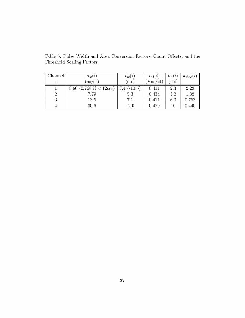
Table 6: Pulse Width and Area Conversion Factors, Count Offsets, and theThreshold Scaling Factors

Channel aw(i) bw(i) aA(i) bA(i) athre(i)i (ns/ct) (cts) (Vns/ct) (cts)

1 3.60 (0.768 if < 12cts) 7.4 (-10.5) 0.411 2.3 2.292 7.79 5.3 0.434 3.2 1.323 13.5 7.1 0.411 6.0 0.7634 30.6 12.0 0.429 10 0.440

27

Figure Captions

Figure 1. MGS spacecraft and MOLA.

Figure 2. Illustration of the MOLA measurement geometry. The drawingassumes that the pointing angle, the pointing error, and the surface normalvectors are all in the same plane.

Figure 3. Timing diagram of the MOLA optical and electrical pulses.

Figure 4. Simplified MOLA receiver blok diagram assuming lossless powersplitter and filters and unity scaling factor for all receiver channels. The filtercharacteristics are listed in Table 4.

Figure 5. The original and the polynominal fit of the inverse Z function.

Figure 6. MOLA Channel 1 ranging error vs. received signal level for 1, 3,10, and 30 degree slope targets.

Figure 7. MOLA Channel 1 Ranging error vs. threshold level normalizedwith respect to pulse amplitude.

Figure 8. MOLA Channel 1 ranging error as a function of range.

28