Marriage Duration and Divorce: The Seven-Year Itchor a Lifelong Itch?

Hill Kulu

# Population Association of America 2014

Abstract Previous studies have shown that the risk of divorce is low during the firstmonths of marriage; it then increases, reaches a maximum, and thereafter begins to decline.Some researchers consider this pattern consistent with the notion of a “seven-year itch,”while others argue that the rising-falling pattern of divorce risk is a consequence ofmisspecification of longitudinal models because of omitted covariates or unobservedheterogeneity. The aim of this study is to investigate the causes of the rising-falling patternof divorce risk. Using register data from Finland and applying multilevel hazard models, theanalysis supports the rising-falling pattern of divorce bymarriage duration: the risk ofmaritaldissolution increases, reaches its peak, and then gradually declines. This pattern persistswhen I control for the sociodemographic characteristics of women and their partners. Theinclusion of unobserved heterogeneity in the model leads to some changes in the shape ofthe baseline risk; however, the rising-falling pattern of the divorce risk persists.

Keywords Divorce .Marriage .Multilevel hazardmodels . Finland

Introduction

An extensive amount of multidisciplinary literature exists on the trends and patterns ofdivorce and separation in industrialized countries (for recent reviews, see Amato 2010;Cherlin 2010; Lyngstad and Jalovaara 2010). An ingredient of longitudinal models ondivorce is the marriage duration. Most studies show that the risk of separation is low duringthe first months of a marriage; it then increases, reaches a maximum, and thereafter beginsto decrease. Various studies on industrialized countries have found this pattern (Andersson1995; Diekmann and Engelhardt 1999; Hoem and Hoem 1992; Jalovaara 2013; Kiernan1999; Kulu and Boyle 2010; Lyngstad 2011; Rootalu 2010; Schoen 1975; Thornton and

DemographyDOI 10.1007/s13524-013-0278-1

Electronic supplementary material The online version of this article (doi:10.1007/s13524-013-0278-1)contains supplementary material, which is available to authorized users.

H. Kulu (*)School of Environmental Sciences, University of Liverpool, Roxby Building, Liverpool, L69 7ZT, UKe-mail: hill.kulu@liverpool.ac.uk

Rodgers 1987). The reason for the rising-falling pattern of divorce risk over the marriageduration, however, has not been discussed much in demographic and sociological studies.Classical psychological literature and public discourse consider this pattern consistent withthe notion of a “seven-year itch.” Most married couples experience a gradual but steadydecline in marital quality after the first year of marriage, suggesting that the short honey-moon period of passion is followed by everyday routine, during which the differencesbetween spouses’ attitudes, values, and behavior become visible and subject to discussionand arguing. This is a period when spouses encourage some behaviors of their partnersand discourage others; at the same time, they try to adapt to those behaviors andcharacteristics of their partners that cannot be easily changed. Experiences arecumulated over time through a mutual learning process, and the couple determineswhether staying together makes sense. If the mutual adaptation is successful, alonger period of stability follows in the marital relationship (Diekmann and Mitter1984; Kurdek 1999; Levinger 1983; Sternberg 1986).

Although the premise of the seven-year itch is convincing, perhaps the rising-fallingpattern of divorce risk is simply produced by misspecification of longitudinal modelson divorce and separation. It is well-known that the baseline risk in hazard models issensitive to model specification (Galler and Poetter 1990; Hoem 1990; Vaupel et al.1979; Vaupel and Yashin 1985). Recent studies reporting the rising-falling pattern ofdivorce over the marriage duration have controlled for a set of demographic andsocioeconomic characteristics of spouses. However, it is likely that some importantcharacteristics of spouses have not been measured and included in the analysis; this isparticularly the case with personality traits of spouses, their values, and their long-termplans. For example, the sample may contain individuals who are prone to divorcebecause of liberal values or because they are ambitious and never satisfied with theircurrent life situation. Similarly, the sample may include individuals who are less proneto divorce because of traditional value beliefs or because they tend to avoid changes intheir lives. Omitting important covariates from the analysis or unobserved heterogene-ity may significantly distort the true shape of the baseline risk: the estimates on the riskof divorce over marriage duration would be downwardly biased. The logic is simple.The high-risk group leaves the risk population first; therefore, as time goes by, the shareof the low-risk group increases, and the hazard of divorce for the population willapproach their (low) risk levels (for details, see Online Resource 1).

The aim of this study is to investigate the causes of the rising-falling pattern ofdivorce risk over the marriage duration. Some literature supports the psychologicalinterpretation (e.g., Diekmann and Engelhardt 1999), and other studies suggest that theunmeasured characteristics of individuals account for the rising-falling pattern of di-vorce risk (e.g., Vaupel and Yashin 1985). However, no study has explicitly controlledfor unobserved heterogeneity when examining the hazard of divorce over the marriageduration. I use a large longitudinal data set from Finland and multilevel hazard regres-sion models, which allow me to identify and control for unobserved heterogeneity.

I first study the hazard of divorce over the marriage duration, controlling for a set ofdemographic and socioeconomic characteristics of women and their partners. I thenidentify and control for possible unobserved heterogeneity to detect any changes in theshape of baseline risk. In further analysis, I examine the hazard of divorce over themarriage duration separately across periods to identify any changes in the shape ofbaseline risk over years.

H. Kulu

Data, Methods, and Modeling Strategy

The data come from the Finnish Longitudinal Fertility Register, a database developed byStatistics Finland that contains linked individual-level information from different admin-istrative registers (see Vikat 2004). I had access to full marital records for 10 % of the(randomly selected) Finnish women born between 1945 and 1983. The data also includefull educational and fertility histories of women and their demographic characteristics(date and place of birth, and native language). In total, 74,441 Finnish women wereincluded in the analysis, excluding foreign-born women (3 %). I linked to women’s datarecords of their husbands; I had information on the men’s educational histories and theirdemographic characteristics. I included in the analysis all marriages for women that wereformed between 1967 and 2000. The database at hand contains no information ondivorces before that period. In total, there were 81,025 marriages: 74,441 first, 6,106second, and 478 third or higher-order marriages (see Table S1 in Online Resource 1). Thenumber of divorces was 18,839: 17,201 for first, 1,498 for second, and 140 for third andsubsequent marriages. I controlled for basic demographic and socioeconomic character-istics of women when investigating the risk of divorce over marital duration (Table 1).

I used a continuous-time event-history model to investigate the hazard of marriagedissolution (Blossfeld and Rohwer 1995; Hoem 1987, 1993). The model was specifiedas follows:

where hij(t) denotes the hazard of separation of jth marriage for woman i. lnh0(t) denotesthe baseline log-hazard, which I specified as a piecewise linear spline. I used thepiecewise linear specification instead of a parametric specification (e.g., a Weibull-distributed baseline) to pick up the baseline log-hazard because the piecewise specifi-cation allows me to easily capture any shape of the baseline hazard. This was critical forthe study, in which the shape of the baseline hazard is the main interest. The value of thelinear spline function between the points (tn, yn) and (tn + 1, yn + 1) was calculated asfollows: y(t) = yn + sn + 1(t – tn) for n = 0, 1, 2, . . ., where sn + 1 is the slope of the linearspline over the interval [tn,tn + 1]. To calculate the linear spline function, I thus definednodes and estimated from the data constant y0 and slope parameters s1, s2, . . . .

The model also included time-constant and time-varying covariates denoted byxijk(t), with parameters measuring their effect. I also included a woman-level residual(or random effect) to control for the time-invariant unmeasured characteristics of awoman (or unobserved heterogeneity) that influenced the hazard of divorce for any ofher marriages. I assumed the woman-level residuals to follow a normal distribution:

The identification of the model was attained through within-person replication. Somewomen had experienced more than one marriage episode; this was sufficient for theidentification of the model with a woman-level random effect or “shared frailty” formarriage episodes (Aalen 1994; Hoem 1990; Hougaard 1995). More specifically, theinformation provided by repeated episodes was used to estimate the variance of therandom effect in the data (rather than individual random effects); the parameters of themodel were estimated conditional on (or along with) the variance of the random effect

(1)

(2)

Marriage Duration and Divorce

Table 1 Person-years and divorces by categories of variables

Person-Years Divorces

Number % Number %

Marriage Duration

0–5 years 366,308.45 32 5,612 30

5–10 years 280,607.55 24 5,687 30

10–15 years 210,177.81 18 3,415 18

15–20 years 150,281.87 13 2,198 12

20–25 years 95,224.49 8 1,365 7

25+ years 52,534.83 5 562 3

Marriage Order

First marriage 1,100,588.27 95 17,201 91

Second marriage 52,166.40 5 1,498 8

Third or subsequent marriage 2,380.33 0.2 140 0.7

Period

≤1974 77,064.99 7 598 3

1975–1979 127,626.51 11 2,123 11

1980–1984 179,675.73 16 2,687 14

1985–1989 223,507.83 19 3,079 16

1990–1994 256,099.42 22 4,612 24

1995+ 291,160.51 25 5,740 30

Age at Marriage

≤19 years 196,414.37 17 4,287 23

20–24 years 607,614.19 53 9,265 49

25–29 years 250,400.00 22 3,576 19

30–34 years 69,934.12 6 1,120 6

35–39 years 21,361.17 2 393 2

40+ years 9,411.15 1 198 1

Language

Finnish 1,096,644.07 95 18,175 96

Swedish 58,490.93 5 664 4

Educational Level

Lower secondary 352,565.30 31 6,739 36

Upper secondary 470,785.46 41 7,766 41

Vocational 212,434.23 18 2,847 15

Lower tertiary 60,630.44 5 727 4

Upper tertiary 58,719.57 5 760 4

Husband’s Educational Level

Lower secondary 382,224.12 33 7,360 39

Upper secondary 455,731.03 39 7,692 41

Vocational 148,613.89 13 1,880 10

Lower tertiary 77,584.92 7 890 5

Upper tertiary 90,981.04 8 1,017 5

Relative Ages of Partners

Husband 5+ years older 168,537.08 15 2,963 16

H. Kulu

(Lillard 1993; Lillard and Panis 2003).1 I thus used a multilevel event-history model tocontrol for unobserved heterogeneity—a strategy that has become common in demo-graphic studies (see Brien et al. 1999; Kulu 2005; Kulu and Steele 2013; Lillard 1993;Lillard et al. 1995; Steele et al. 2006).2

1 I conducted experiments to investigate the sensitivity of residual variance to the share of population withrepeated episodes. As expected, the estimate for the residual variance depended little on how large the share ofpopulation with repeated episodes was (100 %, 50 %, 25 %, 10 %, and 5 %) in the context where the intraclasscorrelation was moderate to strong (i.e., the durations of an individual were positively correlated).2 The identification of the model with unobserved heterogeneity was thus based on the existence of multiplemarriages (and divorces) for some women. It is likely that there were more disruption-prone women (orwomen with unmeasured characteristics that made them disruption-prone) among this group than amongwomen who had been married only once. Therefore, some assumptions of my statistical model might not befully met (e.g., normality of the residuals), and I might overestimate or underestimate the true amount ofheterogeneity in the population (e.g., unmeasured individual values or personality traits that made somewomen more and others less likely of experiencing divorce). However, the proposed approach was the onlyway of estimating unobserved heterogeneity from the data without imposing strong assumptions on data.Alternatively, one could have used all women to identify unobserved heterogeneity; however, this approachwould have required strong assumptions about distribution of both the residuals and the baseline risk (i.e., therisk of divorce by marriage duration), the shape of which is the main interest of this study. My approach wasthus well justified; I also tested sensitivity of the results to underestimation and overestimation of the amountof unobserved heterogeneity in the population (see footnote 3).

Table 1 (continued)

Person-Years Divorces

Number % Number %

Husband 1–4 years older 477,192.67 41 7,547 40

No difference 400,041.94 35 6,184 33

Wife 1+ years older 109,363.31 9 2,145 11

Children

No children 137,261.00 12 3,223 17

One child 324,670.54 28 5,860 31

Two children 477,583.45 41 6,764 36

Three or more children 215,620.02 19 2,992 16

Premarital Conception or Birth

No 666,393.55 58 9,331 50

Conception 375,009.51 32 6,460 34

Birth 113,731.94 10 3,048 16

Age of the Youngest Child

No children 137,261.00 12 3,223 17

Pregnancy 89,437.36 8 495 3

0–2 years 229,894.29 20 1,651 9

2–5 years 215,639.57 19 4,447 24

5–10 years 216,549.71 19 4,531 24

10+ years 266,353.07 23 4,492 24

Total 1,155,135.00 100 18,839 100

Source: Author’s calculations are based on the data from the Finnish Longitudinal Fertility Register.

Marriage Duration and Divorce

Results

In Model 1, I included marriage duration (baseline), marriage order, and period. Asshown in Fig. 1 and Table 2 (Model 1), the hazard of divorce significantly increasedduring the first three years of marriage. In the following two years, the risk furtherincreased and reached its peak at the fifth year of marriage. In the next five years ofmarriage, the risk of separation significantly decreased, and a decline also continuedlater. The analysis thus supports the results of previous studies: a rising-falling patternof divorce risk over the marriage duration, with its peak around the fifth year ofmarriage. The effects of the two covariates were as expected; the hazard of divorceincreased over time (Andersson 1995), and women in their second and third marriageswere more likely to separate than women in their first marriages (Andersson 1995;Hoem and Hoem 1992).

In Model 2, I included a set of sociodemographic characteristics of women and theirpartners. The likelihood ratio (LR) test showed that the model fit improved significantly(LR = 7,829.1, df = 26, p < .001). The effects of covariates were as expected: as shownin Table 2, the hazard of divorce increased with a decrease in the woman’s age atmarriage (cf. Tzeng and Mare 1995); this risk was also higher for couples with a loweducational level (cf. Hoem 1997), for women who spoke Finnish rather than Swedish(cf. Finnäs 1997), and for couples in which the woman was older than the man (cf.Chan and Halpin 2003). As expected, the risk of divorce decreased with an increasingnumber of children in the family. However, the hazard of divorce significantly variedwith the age of the youngest child. The risk of separation decreased substantially whena woman became pregnant; the risk remained low during the pregnancy, around thebirth of a child, and during the first two years of the child’s life; the hazard of divorcegradually increased as the child became older (cf. Erlangsen and Andersson 2001).Couples who experienced a premarital conception or childbirth had a significantlyhigher risk of marital disruption than those whose children had all been conceived andborn in marriage, which was also expected (cf. Hoem 1997). Most importantly,however, the shape of the baseline hazard changed somewhat after controlling forbasic sociodemographic characteristics of couples (see Fig. 1; Table 2, Model 2). Therising-falling pattern became even more pronounced, again consistent with the resultsof previous studies.

In Model 3, I also included a woman-level random residual to control for the effectof her (time-invariant) unmeasured characteristics on the hazard of divorce. I thus

0.0

0.2

0.4

0.6

0.8

1.0

1.2

0 5 10 15 20 25

Rel

ativ

e R

isk

of D

ivor

ce

Years Since Marriage

Model 1 Model 2 Model 3

Fig. 1 Relative risks of divorce by marriage duration. The reference point is at year 5 for each model. Source:Author’s calculations are based on the data from the Finnish Longitudinal Fertility Register

H. Kulu

Table 2 Log-relative risks of divorce (parameter estimates and standard errors in brackets)

Model 1 Model 2 Model 3

Marriage Duration

Constant –7.809** –7.906** –8.283**

(0.179) (0.182) (0.188)

0–1 years (slope) 3.242** 3.577** 3.585**

(0.190) (0.192) (0.192)

1–3 years (slope) 0.293** 0.310** 0.338**

(0.026) (0.026) (0.026)

3–5 years (slope) 0.028 0.005 0.042*

(0.017) (0.018) (0.018)

5–10 years (slope) –0.061** –0.127** –0.106**

(0.007) (0.007) (0.008)

10–15 years (slope) –0.041** –0.097** –0.090**

(0.007) (0.008) (0.008)

15–20 years (slope) –0.010 –0.052** –0.047**

(0.008) (0.009) (0.009)

20+ years (slope) –0.059** –0.090** –0.089**

(0.007) (0.007) (0.007)

Marriage Order

First marriage 0 0 0

Second marriage 0.466** 0.574** 0.257**

(0.028) (0.033) (0.052)

Third or subsequent marriage 1.144** 1.289** 0.643**

(0.086) (0.092) (0.128)

Period

≤1974 –0.513** –0.829** –0.876**

(0.046) (0.047) (0.048)

1975–1979 0.075* –0.095** –0.109**

(0.029) (0.030) (0.030)

1980–1984 0 0 0

1985–1989 –0.047† 0.103** 0.112**

(0.027) (0.027) (0.027)

1990–1994 0.274** 0.575** 0.605**

(0.025) (0.026) (0.027)

1995+ 0.429** 0.855** 0.922**

(0.025) (0.026) (0.029)

Age at Marriage

≤19 years 0.959** 1.076**

(0.027) (0.033)

20–24 years 0.493** 0.540**

(0.021) (0.024)

25–29 years 0 0

Marriage Duration and Divorce

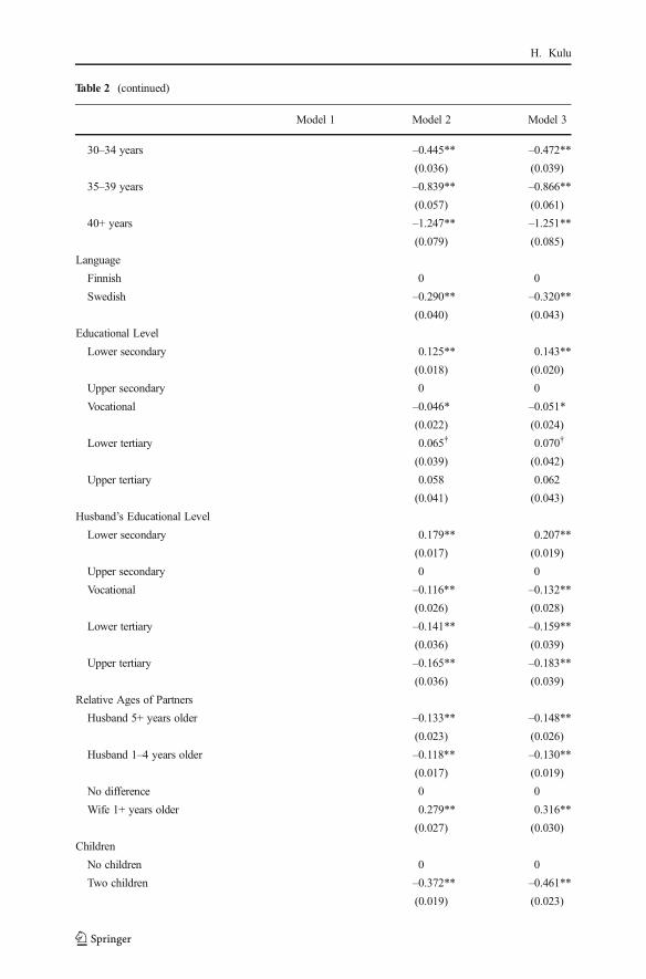
Table 2 (continued)

Model 1 Model 2 Model 3

30–34 years –0.445** –0.472**

(0.036) (0.039)

35–39 years –0.839** –0.866**

(0.057) (0.061)

40+ years –1.247** –1.251**

(0.079) (0.085)

Language

Finnish 0 0

Swedish –0.290** –0.320**

(0.040) (0.043)

Educational Level

Lower secondary 0.125** 0.143**

(0.018) (0.020)

Upper secondary 0 0

Vocational –0.046* –0.051*

(0.022) (0.024)

Lower tertiary 0.065† 0.070†

(0.039) (0.042)

Upper tertiary 0.058 0.062

(0.041) (0.043)

Husband’s Educational Level

Lower secondary 0.179** 0.207**

(0.017) (0.019)

Upper secondary 0 0

Vocational –0.116** –0.132**

(0.026) (0.028)

Lower tertiary –0.141** –0.159**

(0.036) (0.039)

Upper tertiary –0.165** –0.183**

(0.036) (0.039)

Relative Ages of Partners

Husband 5+ years older –0.133** –0.148**

(0.023) (0.026)

Husband 1–4 years older –0.118** –0.130**

(0.017) (0.019)

No difference 0 0

Wife 1+ years older 0.279** 0.316**

(0.027) (0.030)

Children

No children 0 0

Two children –0.372** –0.461**

(0.019) (0.023)

H. Kulu

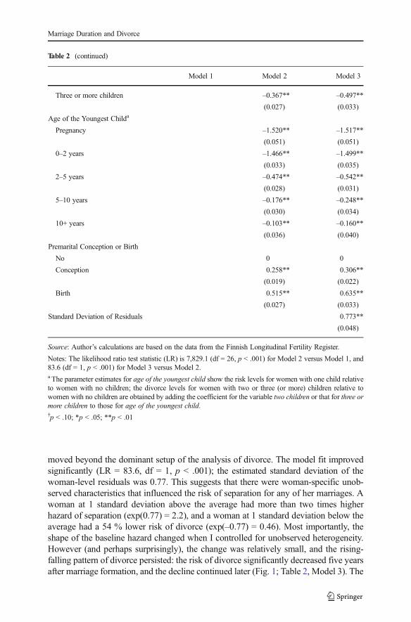
moved beyond the dominant setup of the analysis of divorce. The model fit improvedsignificantly (LR = 83.6, df = 1, p < .001); the estimated standard deviation of thewoman-level residuals was 0.77. This suggests that there were woman-specific unob-served characteristics that influenced the risk of separation for any of her marriages. Awoman at 1 standard deviation above the average had more than two times higherhazard of separation (exp(0.77) = 2.2), and a woman at 1 standard deviation below theaverage had a 54 % lower risk of divorce (exp(–0.77) = 0.46). Most importantly, theshape of the baseline hazard changed when I controlled for unobserved heterogeneity.However (and perhaps surprisingly), the change was relatively small, and the rising-falling pattern of divorce persisted: the risk of divorce significantly decreased five yearsafter marriage formation, and the decline continued later (Fig. 1; Table 2, Model 3). The

Table 2 (continued)

Model 1 Model 2 Model 3

Three or more children –0.367** –0.497**

(0.027) (0.033)

Age of the Youngest Childa

Pregnancy –1.520** –1.517**

(0.051) (0.051)

0–2 years –1.466** –1.499**

(0.033) (0.035)

2–5 years –0.474** –0.542**

(0.028) (0.031)

5–10 years –0.176** –0.248**

(0.030) (0.034)

10+ years –0.103** –0.160**

(0.036) (0.040)

Premarital Conception or Birth

No 0 0

Conception 0.258** 0.306**

(0.019) (0.022)

Birth 0.515** 0.635**

(0.027) (0.033)

Standard Deviation of Residuals 0.773**

(0.048)

Source: Author’s calculations are based on the data from the Finnish Longitudinal Fertility Register.

Notes: The likelihood ratio test statistic (LR) is 7,829.1 (df = 26, p < .001) for Model 2 versus Model 1, and83.6 (df = 1, p < .001) for Model 3 versus Model 2.a The parameter estimates for age of the youngest child show the risk levels for women with one child relativeto women with no children; the divorce levels for women with two or three (or more) children relative towomen with no children are obtained by adding the coefficient for the variable two children or that for three ormore children to those for age of the youngest child.†p < .10; *p < .05; **p < .01

Marriage Duration and Divorce

results thus challenge the idea of the critical role of unmeasured characteristics: after Icontrolled for demographic and socioeconomic characteristics of women and theirpartners, the rising-falling pattern of the hazard of divorce persisted even when I alsocontrolled for unmeasured women’s characteristics. The rising-falling pattern persistedfor two reasons. First, the decline of the hazard after its peak was steep in the model inwhich I controlled for all available (observed) characteristics of women andtheir partners (particularly the age of the youngest child). Second, the estimatedvariance in the heterogeneity term was not large enough to substantially modifythe baseline risk.3

Next, I extended the analysis by investigating the hazard of divorce over themarriage duration across periods to identify any changes in the shape of baseline riskover years. I estimated a model with separate baselines for five periods (until 1979,1980–1984, 1985–1989, 1990–1994, and 1995 and later). The model fit improvedsignificantly (LR = 146.1, df = 22, p < .001), suggesting significant differences in thehazard of divorce over the marriage duration by period. On closer inspection, however,the differences were not fundamental. The shape of the baseline hazard was rathersimilar for the three periods (Fig. 2; Table S2 in Online Resource 1, Model 4).Interestingly, however, the hazard of divorce risk reached its peak sooner inthe 1980s and in the beginning of the 1990s than in the 1970s; the relative riskof divorce at longer marriage durations was also slightly higher in the laterperiods than in earlier periods.

Summary and Discussion

The aim of this study was to investigate the causes of the rising-falling pattern ofdivorce levels. I used a large longitudinal dataset and applied multilevel event-historymodels to control for unobserved heterogeneity when examining the hazard ofdivorce by marriage duration. The initial analysis supported the rising-fallingpattern of divorce by marriage duration: the risk of marital dissolution increased,reached its peak at around the fifth year of marriage, and then gradually declined.This pattern persisted when I controlled for the sociodemographic characteristics ofwomen and their partners and the number of children. The inclusion of unobservedheterogeneity in the model led to changes in the shape of the baseline risk; however,the rising-falling pattern of the divorce risk persisted.

Some issues related to specification of the models and robustness of the results areworthy of discussion. One issue is whether to include in the divorce models marriagecohort or calendar year to measure the effect of social context. Although both model

3 I conducted additional analysis to explore how sensitive the shape of the baseline was to the estimates for theresidual variance/standard deviation. The shape of the baseline became less pronounced with an increase in thevariance/standard deviation, as expected (see Fig. S1 in Online Resource 1). However, the value of 3.0 for thestandard deviation (9.0 for the variance) was needed to substantially modify the shape of the baseline. Thissuggests that a woman with unmeasured characteristics that place her at 1 standard deviation above theaverage had 20 times higher hazard of separation (exp(3.0) = 20.1) than a woman with average unobservedcharacteristics (e.g., in the middle in the liberal-conservative scale), while a woman at 1 standard deviationbelow the average had a 95 % lower risk of divorce (exp(–3.0) = 0.05). Empirical analysis gave no support to(or even no indication of) the existence of such enormous unobserved heterogeneity in the data.

H. Kulu

specifications are correct, there is a clear reason to favor calendar year over marriagecohort if one wishes to distinguish various duration effects from one another. Furtheranalysis revealed that a model with marriage cohort (rather than with calendar year)would have led to the overestimation of the divorce risk at longer marriage durationsbecause of increased divorce rates over years. This suggests that using the calendar yearis a better variable than marriage cohort to measure changes over time in the contextwhere the risk of divorce steadily increases.

Another issue is that the data used in this study contain no information on premaritalcohabitation. However, research shows that cohabitation significantly increased inFinland during the study period: most women born before 1945 started their (first) unionby contracting a marriage, but the majority of those born in the 1960s cohabited beforemarriage (Lindgren et al. 1992). Therefore, it is expected that most marriages in the 1980sand 1990s followed a spell of cohabitation with an average duration of two to three years(Andersson and Philipov 2002:218; Lindgren et al. 1992). As cohabitation graduallyspread during the study period, this may also explain why marriage durations slightlydeclined in the 1980s in comparison with the 1970s. At first glance, this suggests that therisk of separation for relationships reaches its peak a few years later than observed in thedivorce data used. However, the fact that divorce process lasts some time may cancel outthe time that premarital cohabitation adds to the length of the relationship. In Finland, theprocess of divorce usually lasts a year because of a required period of reconsideration afterthe submission of an application for divorce. Further, before 1987, the partners who hadconsidered divorce first had to live separately for a year before their application fordivorce was approved. There is thus a period of a year or so between the timing of adecision to divorce and the date of divorce recorded in statistics.

This study used register data from Finland to investigate the causes of the rising-falling pattern of the divorce risk over the marriage duration. The analysis found nosupport to the idea that the rising-falling pattern is attributed to misspecification of thedivorce models—that is, to the omission of unmeasured (time-invariant) characteristicsof individuals from a model on marital divorce. Future research should study the rolethat the aging of individuals plays in declining divorce rates over the marriage duration.

Acknowledgments The author is grateful to three anonymous referees and former Editor Stewart Tolnay forvaluable comments and suggestions on a previous version of this article. The author also thanks StatisticsFinland for providing the register data used in this study, as well as Mrs. Marianne Johnson for valuable

0.0

0.2

0.4

0.6

0.8

1.0

1.2

0 5 10 15 20 25

Rel

ativ

e R

isk

of D

ivor

ce

Years Since Marriage

19791980–19841985–19891990–19941995+

Fig. 2 Relative risks of divorce by marriage duration and period (Model 4). The reference point is at year 5for each model. Source: Author’s calculations are based on the data from the Finnish Longitudinal FertilityRegister

Marriage Duration and Divorce

suggestions when preparing the data order. The analyses made in this study are based on the Statistics FinlandRegister Data at the Max Planck Institute for Demographic Research (TK-53-1662-05).

References

Aalen, O. O. (1994). Effects of frailty in survival analysis. Statistical Methods in Medical Research, 3, 227–243.

Amato, P. R. (2010). Research on divorce: Continuing trends and new developments. Journal of Marriage andFamily, 72, 650–666.

Andersson, G. (1995). Divorce-risk trends in Sweden 1971–1993. European Journal of Population, 11, 293–311.

Andersson, G., & Philipov, D. (2002). Life-table representations of family dynamics in Sweden, Hungary and14 other FFS countries: A project of description of demographic behaviour. Demographic Research,7(article 4), 67–144. doi:10.4054/DemRes.2002.7.4

Blossfeld, H.-P., & Rohwer, G. (1995). Techniques of event history modeling: New approaches to causalanalysis. Mahwah, NJ: Lawrence Erlbaum Associates.

Brien, M. J., Lillard, L. A., & Waite, L. J. (1999). Interrelated family building behaviors: Cohabitation,marriage, and nonmarital conception. Demography, 36, 531–551.

Chan, T. W., & Halpin, B. (2003). Union dissolution in the United Kingdom. International Journal ofSociology, 32, 76–93.

Cherlin, A. J. (2010). Demographic trends in the United States: A review of research in the 2000s. Journal ofMarriage and Family, 72, 403–409.

Diekmann, A., & Engelhardt, H. (1999). The social inheritance of divorce: Effects of parent’s family type inpostwar Germany. American Sociological Review, 64, 783–793.

Diekmann, A., &Mitter, P. (1984). A comparison of the “sickle function”with alternative stochastic models ofdivorce rates. In A. Diekmann & P. Mitter (Eds.), Stochastic models of social processes (pp. 123–153).Orlando, FL: Academic Press.

Erlangsen, A., & Andersson, G. (2001). The impact of children on divorce risks in first and later marriages(MPIDR Working Paper WP-2001-033). Rostock, Germany: Max Planck Institute for DemographicResearch.

Finnäs, F. (1997). Social integration, heterogeneity, and divorce: The case of the Swedish-speaking populationin Finland. Acta Sociologica, 40, 263–277.

Galler, H. P., & Poetter, U. (1990). Unobserved heterogeneity in models of unemployment duration. In K. U.Mayer & N. B. Tuma (Eds.), Event history analysis in life course research (pp. 226–240). Madison:University of Wisconsin Press.

Hoem, B., & Hoem, J. M. (1992). The disruption of marital and non-marital unions in contemporary Sweden.In J. Trussell, R. Hankinson, & J. Tilton (Eds.), Demographic applications of event history analysis (pp.61–93). Oxford, UK: Clarendon Press.

Hoem, J. M. (1987). Statistical analysis of a multiplicative model and its application to the standardization ofvital rates: A review. International Statistical Review, 55, 119–152.

Hoem, J. M. (1990). Identifiability in hazard models with unobserved heterogeneity: The compatibility of twoapparently contradictory results. Theoretical Population Review, 37, 124–128.

Hoem, J. M. (1993). Classical demographic models of analysis and modern event-history techniques. InIUSSP: 22nd International Population Conference, Montreal, Canada (Vol. 3, pp. 281–291). Paris,France: IUSSP.

Hoem, J. M. (1997). Educational gradients in divorce risks in Sweden in recent decades. Population Studies,51, 19–27.

Hougaard, P. (1995). Frailty models for survival data. Lifetime Data Analysis, 1, 255–273.Jalovaara, M. (2013). Socioeconomic resources and the dissolution of cohabitations and marriages. European

Journal of Population, 29, 167–193.Kiernan, K. (1999). Cohabitation in Western Europe. Population Trends, 96, 25–32.Kulu, H. (2005). Migration and fertility: Competing hypotheses re-examined. European Journal of

Population, 21, 51–87.Kulu, H., & Boyle, P. J. (2010). Premarital cohabitation and divorce: Support for the “trial marriage” theory?

Demographic Research, 23(article 31), 879–904.

H. Kulu

Kulu, H., & Steele, F. (2013). Interrelationships between childbearing and housing transitions in the family lifecourse. Demography, 50, 1687–1714.

Kurdek, L. A. (1999). The nature and predictors of the trajectory of change in marital quality for husbands andwives over the first 10 years of marriage. Development Psychology, 5, 1283–1296.

Levinger, G. (1983). Development and change. In H. H. Kelley, E. Berscheid, A. Christensen, J. H. Harvey, T.L. Huston, G. Levinger, E. McClintock, L. A. Peplau, & D. R. Peterson (Eds.), Close relationships (pp.315–359). New York, NY: Freeman.

Lillard, L. A. (1993). Simultaneous equations for hazards: Marriage duration and fertility timing. Journal ofEconometrics, 56, 189–217.

Lillard, L. A., Brien, M. J., & Waite, L. J. (1995). Premarital cohabitation and subsequent marital dissolution:A matter of self-selection? Demography, 32, 437–457.

Lillard, L. A., & Panis, C. W. A. (2003). aML: Multilevel multiprocess statistical software, version 2.0. LosAngeles, CA: EconWare.

Lindgren, J., Ritamies, M., & Miettinen, A. (1992). Consensual unions and their dissolution among Finnishwomen born in 1938–1969. Yearbook of Population Research in Finland, 30, 33–43.

Lyngstad, T. H. (2011). Does community context have an important impact on divorce risk? A fixed-effectsstudy of twenty Norwegian first-marriage cohorts. European Journal of Population, 27, 57–77.

Lyngstad, T. H., & Jalovaara, M. (2010). A review of the antecedents of union dissolution. DemographicResearch, 23(article 10), 257–292. doi:10.4054/DemRes.2010.23.10

Rootalu, K. (2010). The effect of education on divorce risk in Estonia. Trames: Journal of the Humanities andSocial Sciences, 14, 21–33.

Schoen, R. (1975). California divorce rates by age at first marriage and duration of first marriage. Journal ofMarriage and the Family, 37, 548–555.

Steele, F., Kallis, C., & Joshi, H. (2006). The formation and outcomes of cohabiting and marital partnerships inearly adulthood: The role of previous partnership experience. Journal of the Royal Statistical Society A,169, 757–779.

Sternberg, R. J. (1986). The triangular theory of love. Psychological Review, 93, 119–135.Thornton, A., & Rodgers, W. L. (1987). The influence of individual and historical time on marital dissolution.

Demography, 24, 1–22.Tzeng, J. M., & Mare, R. D. (1995). Labor market and socioeconomic effects on marital stability. Social

Science Research, 24, 329–351.Vaupel, J. W., Manton, K. G., & Stallard, E. (1979). The impact of heterogeneity in individual frailty on the

dynamics of mortality. Demography, 16, 439–454.Vaupel, J. W., & Yashin, A. I. (1985). Heterogeneity’s ruses: Some surprising effects of selection on

population dynamics. The American Statistician, 39, 176–185.Vikat, A. (2004). Women’s labor force attachment and childbearing in Finland. Demographic Research,

Special Collection 3(article 8), 177–212. doi:10.4054/DemRes.0.S8.3

Marriage Duration and Divorce