MARLON MARQUEZ MUSNGI - core.ac.uk fileDEPARTMENT OF MECHANICAL ENGINEERING NATIONAL UNIVERSITY OF...
117
A Study Of The Polishing Process Of A Turbine Blade For Automation MARLON MARQUEZ MUSNGI NATIONAL UNIVERSITY OF SINGAPORE 2006
Transcript of MARLON MARQUEZ MUSNGI - core.ac.uk fileDEPARTMENT OF MECHANICAL ENGINEERING NATIONAL UNIVERSITY OF...

A Study Of The Polishing Process Of A Turbine Blade For
Automation
MARLON MARQUEZ MUSNGI
NATIONAL UNIVERSITY OF SINGAPORE
2006

A Study Of The Polishing Process Of A Turbine Blade For
Automation
Marlon Marquez Musngi
(BS in Manufacturing Engineering and Management)
A THESIS SUBMITTED
FOR THE DEGREE OF MASTER OF ENGINEERING
DEPARTMENT OF MECHANICAL ENGINEERING
NATIONAL UNIVERSITY OF SINGAPORE
2006

i
ACKNOWLEDGEMENTS
I would like to extend my sincerest gratitude to the following people who have
helped me in some way to make this work possible:
First and foremost, to my supervisors, Prof. Marcelo Ang and Prof. Teo Chee
Leong, for their incessant guidance, patience, encouragement and supervision all the
way through the research work,
To AUN/Seed Net, for the scholarship award,
To all my colleagues in the lab and in the MEM Department of DLSU Manila
for sharing their wild, wacky but nevertheless useful ideas,
To my family for providing me with their never-ending support
encouragement and prayers,
To my late father for pushing me to do my best and for believing in me,
And above all, to the Lord Jesus Christ, who has never failed to bring me
countless blessings …

ii
TABLE OF CONTENTS
Acknowledgments . . . . . . . . . . . . . . . . . . . . . . . . . . . . . . . . . . . . . . . . . . i
Contents . . . . . . . . . . . . . . . . . . . . . . . . . . . . . . . . . . . . . . . . . . . . . . . . . ii
Summary . . . . . . . . . . . . . . . . . . . . . . . . . . . . . . . . . . . . . . . . . . . . . . . . . v
List of Figures . . . . . . . . . . . . . . . . . . . . . . . . . . . . . . . . . . . . . . . . . . . vii
Chapter 1 Introduction . . . . . . . . . . . . . . . . . . . . . . . . . . . . . . . . . . . . 1
Section 1.1 Overview . . . . . . . . . . . . . . . . . . . . . . . . . . . . . . . . . . . . . . . . . . . 1
Section 1.2 Related Works . . . . . . . . . . . . . . . . . . . . . . . . . . . . . . . . . . . . . . 2
Section 1.3 Main Objectives . . . . . . . . . . . . . . . . . . . . . . . . . . . . . . . . . . . . . 3
Section 1.4 Potential Applications/Exploitations . . . . . . . . . . . . . . . . . . . . . 3
Section 1.5 Thesis Outline . . . . . . . . . . . . . . . . . . . . . . . . . . . . . . . . . . . . . . . 3
Chapter 2 Design of the Experimental Study . . . . . . . . . . . . . . . . . . . 6
Section 2.1 Overall description . . . . . . . . . . . . . . . . . . . . . . . . . . . . . . . . . . . 6
Section 2.2 The Turbine Blade . . . . . . . . . . . . . . . . . . . . . . . . . . . . . . . . . . . 8
Section 2.3 The Hardware . . . . . . . . . . . . . . . . . . . . . . . . . . . . . . . . . . . . . . 10
Section 2.3.1 The Polisher . . . . . . . . . . . . . . . . . . . . . . . . . . . . . . . . 10
Section 2.3.2 The JR3 Force Torque Sensor . . . . . . . . . . . . . . . . . 11
Section 2.3.3 The Polaris . . . . . . . . . . . . . . . . . . . . . . . . . . . . . . . . . 12
Section 2.3.4 The Host Computer . . . . . . . . . . . . . . . . . . . . . . . . . . 13
Section 2.4 The Software . . . . . . . . . . . . . . . . . . . . . . . . . . . . . . . . . . . . . . . 13
Section 2.4.1 The Main MFC Application . . . . . . . . . . . . . . . . . . . 13

iii
Section 2.4.2 The Main RTSS Application . . . . . . . . . . . . . . . . . . . 14
Chapter 3 Force Sensing . . . . . . . . . . . . . . . . . . . . . . . . . . . . . . . . . . . 16
Section 3.1 Initial Ideas . . . . . . . . . . . . . . . . . . . . . . . . . . . . . . . . . . . . . . . . 16
Section 3.1.1 Attaching sensor to the fixture to hold workpiece. . 17
Section 3.1.2 Attaching sensor to the bottom of the polisher . . . . 17
Section 3.2 Current Setup . . . . . . . . . . . . . . . . . . . . . . . . . . . . . . . . . . . . . . 18
Section 3.3 Software Codes . . . . . . . . . . . . . . . . . . . . . . . . . . . . . . . . . . . . . 19
Section 3.4 Data Gathered . . . . . . . . . . . . . . . . . . . . . . . . . . . . . . . . . . . . . . 20
Section 3.5 Need for Filtering . . . . . . . . . . . . . . . . . . . . . . . . . . . . . . . . . . . 21
Section 3.5.1 Getting the Frequency of the desired data . . . . . . . 21
Section 3.5.2 Designing the filter . . . . . . . . . . . . . . . . . . . . . . . . . . 22
Section 3.5.3 Results from filter . . . . . . . . . . . . . . . . . . . . . . . . . . . 23
Chapter 4 Motion Capture . . . . . . . . . . . . . . . . . . . . . . . . . . . . . . . . . 25
Section 4.1 Initial Ideas . . . . . . . . . . . . . . . . . . . . . . . . . . . . . . . . . . . . . . . . 25
Section 4.1.1 Using Laser Tracking System . . . . . . . . . . . . . . . . . . 26
Section 4.1.2 Using Machine Vision . . . . . . . . . . . . . . . . . . . . . . . . 26
Section 4.1.3 Using Phantom Desktop . . . . . . . . . . . . . . . . . . . . . . 27
Section 4.2 Current Setup . . . . . . . . . . . . . . . . . . . . . . . . . . . . . . . . . . . . . . 28
Section 4.3 Software Codes . . . . . . . . . . . . . . . . . . . . . . . . . . . . . . . . . . . . . 29
Section 4.4 Data Gathered . . . . . . . . . . . . . . . . . . . . . . . . . . . . . . . . . . . . . . 30
Chapter 5 Data Analysis . . . . . . . . . . . . . . . . . . . . . . . . . . . . . . . . . . . 31
Section 5.1 Data Transformation . . . . . . . . . . . . . . . . . . . . . . . . . . . . . . . . 31
Section 5.1.1 Orientation Data . . . . . . . . . . . . . . . . . . . . . . . . . . . . 33
Section 5.1.2 Position Data . . . . . . . . . . . . . . . . . . . . . . . . . . . . . . . 34
Section 5.1.3 Force Data . . . . . . . . . . . . . . . . . . . . . . . . . . . . . . . . . 35
iv
Section 5.1.4 Moment Data . . . . . . . . . . . . . . . . . . . . . . . . . . . . . . . 36
Section 5.2 Analysis of the Need of Force and Motion Control . . . . . . . . 36
Chapter 6 Recommendations for Compliant Motion Required for
Poloshing. . . . . . . . . . . . . . . . . . . . . . . . . . . . . . . . . . . . . . . . . . . . . . . . 39
Section 6.1 Amount of Force and Motion Needed . . . . . . . . . . . . . . . . . . 39
Section 6.2 When to Use Force and Motion Control . . . . . . . . . . . . . . . . 40
Chapter 7 Conclusion . . . . . . . . . . . . . . . . . . . . . . . . . . . . . . . . . . . . . 43
References . . . . . . . . . . . . . . . . . . . . . . . . . . . . . . . . . . . . . . . . . . . . . . 45
Appendix A . . . . . . . . . . . . . . . . . . . . . . . . . . . . . . . . . . . . . . . . . . . . . . 49
Appendix B . . . . . . . . . . . . . . . . . . . . . . . . . . . . . . . . . . . . . . . . . . . . . . 54
Appendix C . . . . . . . . . . . . . . . . . . . . . . . . . . . . . . . . . . . . . . . . . . . . . . 81
List

v
SUMMARY
With Airfoil Technologies Singapore (ATS) as partner, a plan to develop an
automated robotic polishing system using motion and force control is proposed. Aside
from technological and research advancements to be gained especially in the field
imitating human motions, the system would be able to perform the polishing job more
consistently resulting in better accuracy and at a faster rate.
In this research, the parameters involved in doing the polishing process are
investigated. Experiments are done to study the motion and forces required to do the
task of polishing turbine blades. The data gathered from these experimentations
are then analyzed to come up with the independent parameters a robot would need to
accomplish the task using motion and force control with respect to the end-effector.
The polisher used is a 4” belt and 6” disc sander. It is driven by an induction
motor running at 220V and giving out 1/3 Horsepower. The upper part of the polisher
was modified in order to accommodate the positioning of the force-torque sensor.
A 6-dof JR3 force-torque sensor is used and is attached to the polisher to
gather the force information of the polishing process. It is attached near the roller
where the belt revolves on. It is placed in a position where all the forces from the
polishing process can be captured with the minimum noise and obstruction.

vi
Motion of the workpiece is captured using a device called the Polaris. Using a
small rod fixture to connect the workpiece and the Polaris tool marker, position and
orientation are recorded through infrared light-emitting diodes fed back by the tool
marker to the Polaris Position Sensor. The fixture is designed in such a way that it
gives minimum or no disturbance at all to the worker while doing the polishing
process.
The data for both force and motion are gathered while a worker from ATS
performs the actual polishing process. This information from the sensors is sent to a
computer at a constant sampling rate of 10 Hz in real time. The analyses of these data
are then used to identify 6 independent force and motion parameters needed by a
robot to perform the task.

vii
LIST OF FIGURES
Figure 2.1 Overall description of setup with connections with location of reference
frames
Figure 2.2 The Turbine Blade
Figure 2.3 Turbine blade connected to the designed fixture
Figure 2.4 The turbine blade connected to the designed fixture held by the hand
Figure 2.5 The polisher with the modified part to accommodate the JR3 FT sensor
Figure 2.6 The main dialog window of the software
Figure 3.1 Graph of the freq. power distribution of data with polish and data w/o polish
Figure 3.2 Design of the 15th Order Butterworth filter with cutoff frequency at 0.5 Hz
Figure 3.3 Graph of the filtered and unfiltered FT Data
Figure 4.1 The Polaris active tool marker attached to the designed fixture
Figure 5.1 Reference frames of different reference points
Figure 5.2 Location of points A& B and their orientation
Figure 5.3 Graph of FT and POSE data (Trial 1)
Figure 5.4 Graph of FT and POSE data (Trial 2)
Figure 5.5 Graph of FT and POSE data (Trial 3)
Figure 6.1 Force and motion frequency (Trial 1)
Figure 6.2 Force and motion frequency (Trial 2)
Figure 6.2 Force and motion frequency (Trial 2)
1
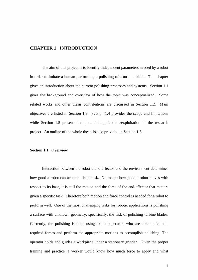
CHAPTER 1 INTRODUCTION
The aim of this project is to identify independent parameters needed by a robot
in order to imitate a human performing a polishing of a turbine blade. This chapter
gives an introduction about the current polishing processes and systems. Section 1.1
gives the background and overview of how the topic was conceptualized. Some
related works and other thesis contributions are discussed in Section 1.2. Main
objectives are listed in Section 1.3. Section 1.4 provides the scope and limitations
while Section 1.5 presents the potential applications/exploitation of the research
project. An outline of the whole thesis is also provided in Section 1.6.
Section 1.1 Overview
Interaction between the robot’s end-effector and the environment determines
how good a robot can accomplish its task. No matter how good a robot moves with
respect to its base, it is still the motion and the force of the end-effector that matters
given a specific task. Therefore both motion and force control is needed for a robot to
perform well. One of the most challenging tasks for robotic applications is polishing
a surface with unknown geometry, specifically, the task of polishing turbine blades.
Currently, the polishing is done using skilled operators who are able to feel the
required forces and perform the appropriate motions to accomplish polishing. The
operator holds and guides a workpiece under a stationary grinder. Given the proper
training and practice, a worker would know how much force to apply and what

2
motions are required so that the workpiece is properly ground and polished. However,
training and practice could take too much time. They develop the skills through years
of experience. Such skilled operators are hard to come by and new operators have to
be trained and they learn and improve themselves through experience. We believe an
automated system would be able to perform the polishing job more consistently
resulting in better accuracy and at a faster rate.
Section 1.2 Related Works
In 1987, it was Dr. Oussama Khatib who first formulated the operational space
formulation, which is a unified approach for motion and force control of robot
manipulators. Since then, this new method of controlling robots, wherein the task is
described in terms of motion and forces in “operational space”, or the space where the
workpiece is in contact with the polishing tool, has been used by many other
researchers. One of them, Dr. Marcelo H. Ang Jr., together with Rodrigo Jamisola,
Denny Oetomo, Tao Ming Lim and Ser Yong Lim, implemented the operational space
formulation to aircraft canopy polishing in 2002.
In 1999, XQ Chen, ZM Gong, H Huang, L Zhou, SS Ge, Q Zhu, and LC
Woon developed an automated 3D Robotic Polishing System for Repairing Turbine
Airfoils. This system first checks on the profile of the turbine then uses an Adaptive
Robot Path Planner to generate the robot blending path and programs.

3
Section 1.3 Main Objectives
• Evaluate the feasibility of using motion and force control in automating the
polishing process
• Gather general motion and force information involved in polishing a turbine
blade
• Identify the independent parameters from which all the motion and force
information is dependent on
• Analyze and generalize a pattern for the independent parameters in doing the
polishing process
• Prepare the foundations for the development of actual system.
Section 1.4 Potential Applications/Exploitation
The developed system will be directly applicable to Airfoil Technologies
Singapore since this is one of the tasks their workers do everyday. They do polishing
of these turbine blades for aircraft repair. Aside from the fact that this will be a big
step in the advancement of robotic machining, upon verification of feasibility, this
could be the foundation for future polishing machine that can be commercialized and
marketed worldwide.
Section 1.5 Thesis Outline
This thesis is divided into 6 chapters.

4
Chapter 2 is on the Experimental Setup. In this chapter, the description of the
various hardware and software used is given in detail. The connection and
coordination of the different hardware to each other and to the software is also
discussed here.
Chapter 3 talks about the force sensing. This chapter basically discusses how
the force/torque information was gathered. The different setups that were thought of
and considered are described here as well. There is also a part in this chapter that
discusses the software code used to communicate with the sensor.
Chapter 4 discusses how the motion capture was done. All the ideas that were
deliberated on and tried are given in this chapter. Same as in chapter 3, some
software codes used to communicate with the hardware are also described here.
Chapter 5 is on Data Analysis. This is the part where the data from force
sensing and motion capture is presented, analyzed and put together. Filtration of
noise, vibration and other unnecessary data are discussed here. The relationship
between each data parameter is observed. This is where all the data is summarized
into independent parameters
Chapter 6 concludes the thesis and makes recommendation for further studies.

5
Competitive Advantage
It should be notable that people, who have actually developed and used this
new method of control and also have experience and knowledge in polishing
automation, are involved in this project. Also, add to this that Airfoil Technologies
Singapore, which does these polishings, is also a partner in doing the project.
Unlike other robotic polishing system developed by other researchers like the
Polishing Robot with Human Friendly Joystick Teaching System developed by
Fusaomi Nagata and Keigo Watanabe in 2000, the proposed system is fully automatic
such that the user would just be “overseeing” the task using a robot-man interface.
Also, in the proposed project, the robot manipulator would be pushing the workpiece
against a stationary belt grinder as apposed to usual polishing systems like the aircraft
canopy polishing system above where the robot manipulator pushes the grinder
against the canopy surface.
In 1999, XQ Chen, ZM Gong, H Huang, L Zhou, SS Ge, Q Zhu, and LC
Woon developed an automated 3D Robotic Polishing System for Repairing Turbine
Airfoils. This system is different from the proposed system in such a way that it first
checks on the profile of the turbine and then uses an Adaptive Robot Path Planner to
generate the robot blending path and programs while the latter uses force feedback to
obtain force control.

6
CHAPTER 2 DESIGN OF THE EXPERIMENTAL STUDY
The main concern for the setup is to be able to gather force and motion of the
polishing process. This means motion of the blade and the force it applies has to be
recorded simultaneously while doing the polishing with the least disturbance to the
polisher operator.
This chapter discusses the setup of the hardware and software used in the
experiment. Section 2.1 is about the overall description of the setup. It illustrates the
setup for experimentation and how the devices are connected with each other. Section
2.2 describes the blade to be polished and the fixtures designed to hold it. Section 2.3
deals with the hardware setup while Section 2.4 provides information about the
software setup.
Section 2.1 Overall Description
The experiment is setup in such a way that all the devices needed must be
working together with one another and thus connected with each other.
The computer is where the user or the host communicates with the system.
The software developed is the interface between the user and the computer. The
computer is connected to the two sensors for it to send and receive data. The JR3 FT
Sensor is connected to the computer through the card receiver which is inserted into
7
the ISA slot of the motherboard. The Polaris connects to the computer via the RS-232
serial port.
The JR3 FT sensor is attached to the polisher as described in Section 2.3.1.
This way, when the workpiece comes in contact with the polisher, the JR3 FT sensor
would be able to sense it.
The workpiece, held by the fixture described in Section 2.2, is connected to
the Active tool marker of the Polaris. This tool marker which is connected to the
Polaris Tool Interface Unit (TIU), will be the one to emit infra-red light that would be
received by the Polaris Position Sensor. Figure 2.1 shows these connections.
computer Polaris TIU
Top view of Polaris position sensor
1000 mm
To serial port
JR3 FT sensor
To card receiver
To TIU
Workpiece with fixture and active tool marker
To active tool marker Top view of polisher
Figure 2.1 Overall description of setup with connections with location of reference frames

8
Section 2.2 The Turbine Blade
The turbine blade came from Airfoil Technologies Singapore, the company
which actually does the polishing of these blades through the help of Mr. Lee Ngan
Ming. The size is around 10mm x 12 mm x 30 mm. It is uniquely shaped in such a
way that the upper part is slightly curved and this curve is further twisted slightly.
Figure 2.2 shows two blades, one without the weld, and the other with some polishing
done on the weld already.
Figure 2.2 The Turbine Blade
Since the objective of the experiment is to be able to gather force and motion
data while polishing with minimal disturbance to the worker, a fixture is designed to
hold the workpiece (blade) and to connect it to the other hardware used for data
gathering. In designing the fixture, the major consideration is for the worker to be to
hold the workpiece almost the same way with or without the fixture.

9
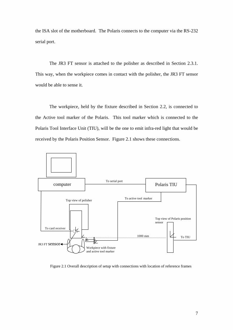
Since the worker holds the workpiece mainly with his or her 2 fingers (thumb
and pointing finger) and with the fist in a some sort of semi-clenched position, it was
decided to design some sort of a rod that would go through the inside of the semi-
clenched fist to connect to the desired measuring device. To secure the workpiece in
place, a sort of cap with a slit on its cover was also designed. Figure 2.3 shows the
designed fixture with a blade with weld attached to it. Figure 2.4 shows how this
fixture is held by the hand.
Figure 2.3 Turbine blade connected to the designed fixture
10
Figure 2.4 The turbine blade connected to the designed fixture held by the hand
Section 2.3 The Hardware
There are a total of four (4) machines/hardware used in the experiment, each
connected to the other. This section describes the function of each part.
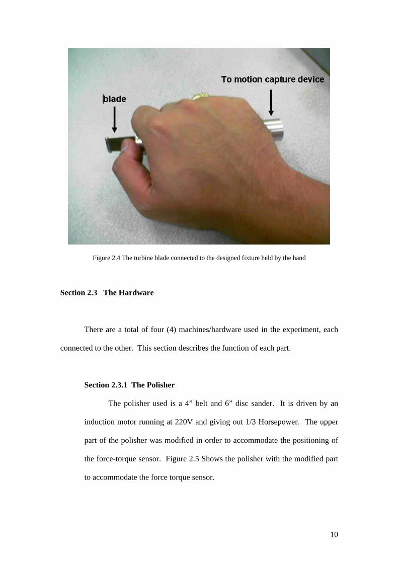
Section 2.3.1 The Polisher
The polisher used is a 4” belt and 6” disc sander. It is driven by an
induction motor running at 220V and giving out 1/3 Horsepower. The upper
part of the polisher was modified in order to accommodate the positioning of
the force-torque sensor. Figure 2.5 Shows the polisher with the modified part
to accommodate the force torque sensor.

11
Figure 2.5 The polisher with the modified part to accommodate the JR3 FT sensor
Section 2.3.2 The JR3 Force-Torque sensor
The JR3 Force Torque sensor provides 6 degree-of freedom force and
torque data at very high bandwidths. Employing an Analog Devices ADSP-
21xx family digital signal processing chip, the JR3 system can provide
decoupled and digitally filtered data at 8 kHz per channel. It is connected to
the JR3 DSP based bus compatible receiver of the ISA (IBM-AT) bus version.
The board, consisting of the Digital Signal Processor, also has shared dual-
ported address space of 16k 2 byte words to which both the host and the DSP
can read and write. Use of the dual ported RAM allows the host to read data
from the DSP with very little overhead. It also allows the host to reconfigure
the DSP on the fly, by writing configuration commands to the RAM.
12
The ISA (IBM-AT) bus receiver card, which plugs into a 16 bit slot on
the ISA bus, uses both the 62 pin and the 36 pin connector. The receiver
occupies 4 consecutive I/O addresses in the range of 000 to 3FF hexadecimal.
The base address is selected by dip switches on the card. The two lower I/O
addresses form a 16 bit address register, the two upper addresses form a 16 bit
data register. The address to be read or written (in the dual port shared address
space) is written to the address register; the data is then read from or written to
the data register.
Section 2.3.3 The Polaris
The Polaris System determines real-time position and orientation by
measuring the 3D positions of markers affixed to both wired and wireless
tools. The system used in this experiment uses a Position Sensor that detects
retro-reflective optical markers, calculates the 3D/6D position of a tool; and
reports the result via a serial interface to the host computer. The tool the
sensor detects consists of 4 active markers mounted on a planar rigid body.
The Polaris system tracks wired active tools with infrared light-
emitting diodes. Active markers emit infrared light which is received by the
position sensor. The position sensor receives light from marker reflections
and marker emissions, respectively. The Polaris system triangulates the 3D
position and orientation of a tool to provide 6 Degrees of Freedom.
13
The 3D position of the target point is calculated from the measured
position and the orientation of the rigid body is defined by the markers.
Section 2.3.4 The Host Computer
The host computer used in the setup is an Intel Pentium II 400MHz
processor with 320MB RAM. It has at least one ISA slot for the JR3 receiver.
It also runs under Microsoft Windows 2000 with RTX extension.
Section 2.4 The Software
The main software used in this project is Microsoft Visual C++. It runs under
Microsoft Windows 2000 with RTX extension. The software is actually divided into
2 parts, the Main MFC Dialog and the Main RTSS application.
Section 2.4.1 The Main MFC Dialog
The Main MFC Dialog is the user interface part of the software. This
is the part where the hardware is initialized. This is also where the shared
memory (also to be used by the RTSS Application) and real time timer is
created.
The dialog window is divided into 4 parts, the Control part, where the
buttons are located for initializing and starting the data gathering procedure;
the Force and Torque part, where the force and torque readings are displayed
and graphed; the POSE part, where position and orientation readings are
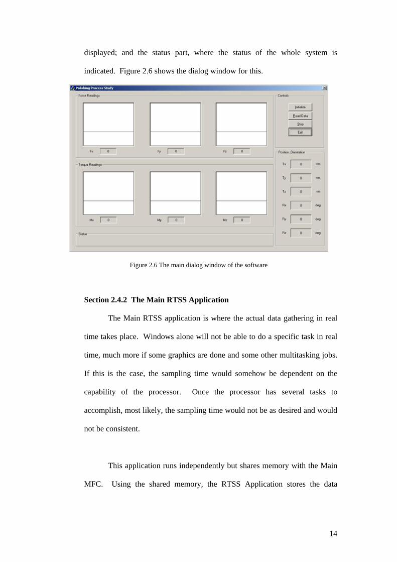
14
displayed; and the status part, where the status of the whole system is
indicated. Figure 2.6 shows the dialog window for this.
Figure 2.6 The main dialog window of the software
Section 2.4.2 The Main RTSS Application
The Main RTSS application is where the actual data gathering in real
time takes place. Windows alone will not be able to do a specific task in real
time, much more if some graphics are done and some other multitasking jobs.
If this is the case, the sampling time would somehow be dependent on the
capability of the processor. Once the processor has several tasks to
accomplish, most likely, the sampling time would not be as desired and would
not be consistent.
This application runs independently but shares memory with the Main
MFC. Using the shared memory, the RTSS Application stores the data

15
gathered for which the MAIN MFC can access and download to show and
graph the data in the dialog window.

16
CHAPTER 3 FORCE SENSING
Knowing what kinds of forces are involved in the polishing process helps in
achieving better and faster polishing results since the exact amount and direction of
the force can be applied. This minimizes or even eliminates unnecessary work plus
excess cutting or polishing is avoided.
This chapter discusses everything about force sensing that was done in the
experiment. Section 3.1 describes the initial ideas that were thought of on where to
put the sensor. It also discusses the pros and cons of each idea. Section 3.2 shows the
accepted setup for force sensing. Some software codes are given in Section 3.3, and
the data gathered from force sensing is explained in section 3.4. Since noise is
inevitable in this situation, Section 3.5 gives the details why filtering would be
needed.
Section 3.1 Initial Ideas
Having already a JR3 FT sensor at hand, the problem was how to get the
needed data. Several ideas were thought of regarding where to attach the sensor in
order for us to get accurate data. This section presents some of these significant ideas.

17
Section 3.1.1 Attaching sensor to the fixture to hold workpiece
One of the ideas was to attach the JR3 FT Sensor to a fixture that
would hold the workpiece. Attaching it to the workpiece itself would not be
possible since the workpiece is too small and that the sensor has no capability
of holding such a thing thus designing a fixture is unavoidable here. In effect,
the worker would then be holding the sensor instead of the workpiece itself
when doing the polishing.
The advantage of using this setup is that very minimal outside forces
will be included in the sensor readings. The sensor would actually be reading
the forces that are applied by the worker to the workpiece and that of the
workpiece to the worker.
The main disadvantage here is that the work or action of the worker in
this setup might not be the same as that of the actual action in the factory since
he/she is not holding the workpiece itself. Minimal obstruction is desired.
Section 3.1.2 Attaching sensor to the bottom of the polisher
Another proposed setup was to attach the JR3 FT sensor to the bottom
of the polisher. This means that the sensor would be in between the polisher
and a solid and fixed base. No other fixtures are needed here just as long as
one side of the sensor is attached firmly to the base and the other to the bottom
of the polisher.

18
The advantage here is that the worker will not be holding anything else
other than the workpiece. Also, since the sensor is also attached to a fixed
base, all forces that are caused by any contact to the polisher (i.e. contact
between workpiece and polisher) would be included in the sensor readings.
The main disadvantage is that the sensor would actually have to carry
the weight of the whole polisher which is quite heavy. Also, when the
polisher is turned on, vibrations are expected. Since the sensor also reads the
force contributed by the weight of the polisher plus the vibrations, the noise or
unwanted force signals might eclipse the force data that is actually needed.
Section 3.2 Current Setup
Based on the idea of attaching the sensor to the base of the polisher to sense
any contact made, a place had to be thought of where the sensor would not be
supporting too much weight but still maintain the ability to sense any contact made
with the polisher. It was then realized that only the contact between the polisher and
the workpiece is actually needed so it was only logical to concentrate on this contact
area. Finally a decision was made and this is to attach the sensor to the part that holds
the roller where the polishing belt revolves on which is actually the desired contact
area. Vibrations are still expected to happen but since the polisher is not supporting
the weight of the whole polisher anymore, it is likely that the noise caused by these
vibrations would not drown out the desired force signal readings

19
In order to attach the sensor to the desired spot, slight modifications were
made to the upper part of the polisher as can be seen in Figure 2.5. This is to
accommodate the size of the sensor.
Section 3.3 Software Codes
The JR3 FT Sensor is connected to the computer through an ISA (IBM-AT)
bus receiver card. The base address is selected by dip switches on the card, in this
case, 0x0314. It has two lower I/O addresses forming a 16 bit address register, and
two upper addresses forming a 16 bit data register. The address to be read or written
(in the dual port shared address space) is written to the address register; the data is
then read from or written to the data register. C++ programming was used to read and
write data for communication.
In reading data from the data register, the address must first be written to the
address register in order for the receiver card to know which data is to be read. For
this, a function called short getdata (int baseadd, int addr) was constructed. In this
function, the address to be read is written on the base address of the card. Then after
some delay for the bus, the data where the given address is located can now be read at
an address that is 2 bytes away from the base address.
short getdata (int baseadd, int addr) {
OUTPORT(baseadd, addr); /*write location to read*/ delay1(); delay1(); /*delay for bus*/ return (INPORT(baseadd+2)); /*read data at addr*/
}
20
Writing data is pretty much the same with reading data. First the base address
must know which address is to be written to, and then the data is written. The
function called void wrtdata (int baseadd, int addr, int val) was constructed for this.
Just like in short getdata (int baseadd, int addr), after some delay for the bus, the data
is written at an address 2 bytes away from the base address. The receiver card then
puts this data to the address that was given to the base address.
void wrtdata (int baseadd, int addr, int val) { OUTPORT(baseadd, addr); delay1(); delay1(); OUTPORT(baseadd+2, val); }
The short getdata (int baseadd, int addr) function is used when data such as
the unfiltered FT data are to be read. The void wrtdata (int baseadd, int addr, int val)
function is used when initializations are to be done, such as zeroing the offsets (zero
output at current loads) or changing the scales. Addresses for specific commands and
data are given in the JR3 FT Sensor Manual & Programming Guide.
Section 3.4 Data Gathered
The data gathered from the FT sensor are raw, unfiltered data. These numbers
which are in Newtons, represent the exact forces that the sensor is able to feel at a
particular time and at the place where the sensor is located. However, the present
form of the data is not suitable in this study. First of all, these data include forces
arising from vibrations of the polisher. These forces, which we would be referring to
as noises, would have to be eliminated in order to get the desired forces and moments
which are directly involved in the polishing process. Also, the study needs forces
21
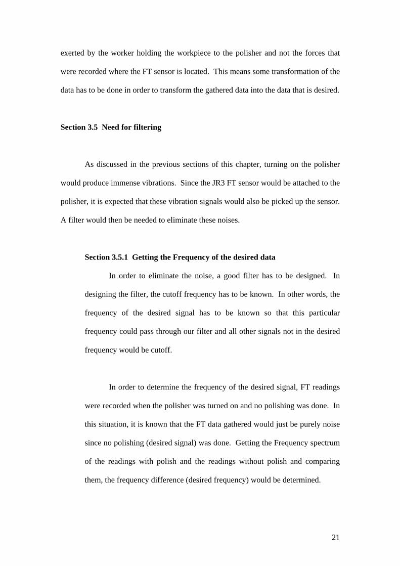
exerted by the worker holding the workpiece to the polisher and not the forces that
were recorded where the FT sensor is located. This means some transformation of the
data has to be done in order to transform the gathered data into the data that is desired.
Section 3.5 Need for filtering
As discussed in the previous sections of this chapter, turning on the polisher
would produce immense vibrations. Since the JR3 FT sensor would be attached to the
polisher, it is expected that these vibration signals would also be picked up the sensor.
A filter would then be needed to eliminate these noises.
Section 3.5.1 Getting the Frequency of the desired data
In order to eliminate the noise, a good filter has to be designed. In
designing the filter, the cutoff frequency has to be known. In other words, the
frequency of the desired signal has to be known so that this particular
frequency could pass through our filter and all other signals not in the desired
frequency would be cutoff.
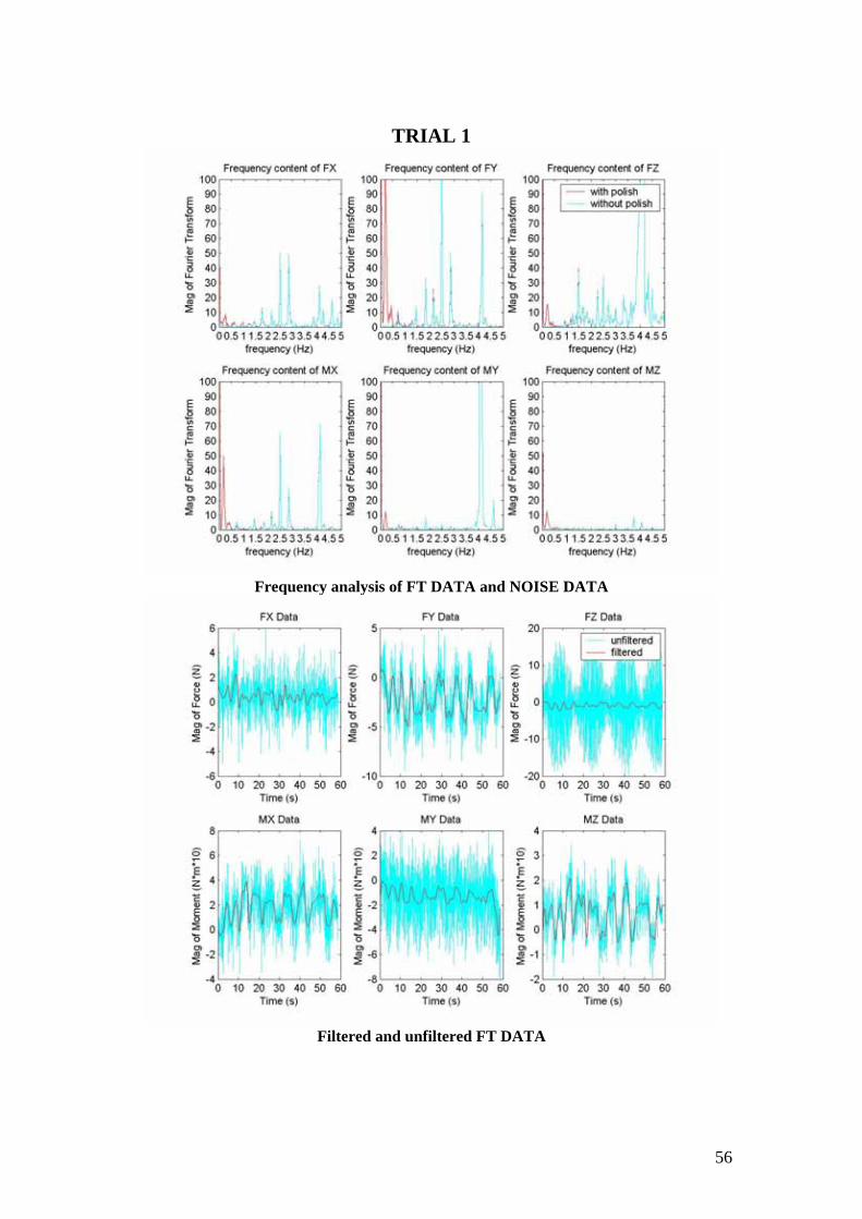
In order to determine the frequency of the desired signal, FT readings
were recorded when the polisher was turned on and no polishing was done. In
this situation, it is known that the FT data gathered would just be purely noise
since no polishing (desired signal) was done. Getting the Frequency spectrum
of the readings with polish and the readings without polish and comparing
them, the frequency difference (desired frequency) would be determined.
22
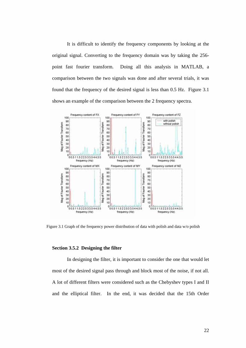
It is difficult to identify the frequency components by looking at the
original signal. Converting to the frequency domain was by taking the 256-
point fast fourier transform. Doing all this analysis in MATLAB, a
comparison between the two signals was done and after several trials, it was
found that the frequency of the desired signal is less than 0.5 Hz. Figure 3.1
shows an example of the comparison between the 2 frequency spectra.
Figure 3.1 Graph of the frequency power distribution of data with polish and data w/o polish
Section 3.5.2 Designing the filter
In designing the filter, it is important to consider the one that would let
most of the desired signal pass through and block most of the noise, if not all.
A lot of different filters were considered such as the Chebyshev types I and II
and the elliptical filter. In the end, it was decided that the 15th Order
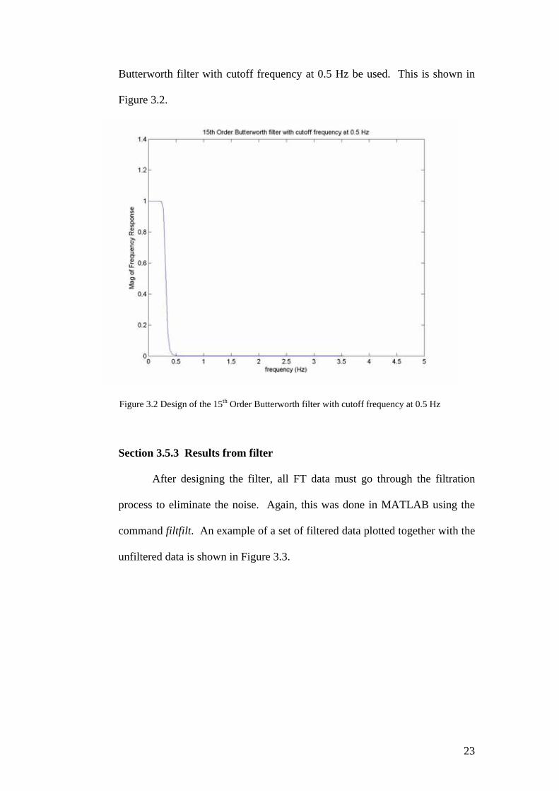
23
Butterworth filter with cutoff frequency at 0.5 Hz be used. This is shown in
Figure 3.2.
Figure 3.2 Design of the 15th Order Butterworth filter with cutoff frequency at 0.5 Hz
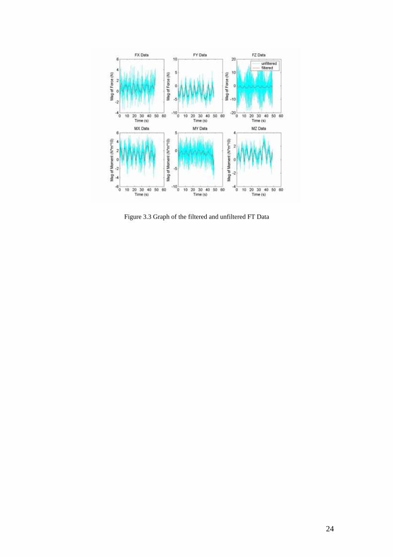
Section 3.5.3 Results from filter
After designing the filter, all FT data must go through the filtration
process to eliminate the noise. Again, this was done in MATLAB using the
command filtfilt. An example of a set of filtered data plotted together with the
unfiltered data is shown in Figure 3.3.
24
Figure 3.3 Graph of the filtered and unfiltered FT Data

25
CHAPTER 4 MOTION CAPTURE
Knowing the motion involved in the polishing process helps in achieving
better and faster polishing automation since this very same motion would be the one
imitated by a robot. With the desired motion known, the trajectory or path of the
robot arm can be computed.
This chapter discusses everything about motion capture that was done in the
experiment. Section 4.1 describes the initial ideas that were thought of on how to
capture the polishing motion. It also discusses the pros and cons of each idea.
Section 4.2 shows the accepted setup for motion capture. Some software codes are
given in Section 4.3, and the data gathered from motion capture is explained in
section 4.4.
Section 4.1 Initial Ideas
Recording the motion of the workpiece undergoing the polishing process was
very tricky. The thing that made it very difficult is the fact that this motion recording
or capturing has to be done with minimal or no interference to the worker. Presented
are some of the initial ideas that were thought of in capturing the motion of the
workpiece undergoing the polishing process.
26
Section 4.1.1 Using Laser Tracking System
The idea of using a laser tracking system got in the picture when it was
found out that it can feedback the 3D position of an object using laser and a
retroflector device. Initially, it was a good idea since communication with the
retroflector where the workpiece would be attached to and the main sensor
would be wireless. Then it was found out that this machine can only give
position and not the orientation of an object at a specific time. So the idea of
attaching at least three (3) retroflectors to the workpiece came into place to be
able to compute for the orientation at any time. However, it was also found
out that the machine can only handle one (1) retroflector at a time so this idea
was eventually rejected.
Section 4.1.2 Using Machine Vision
Another wireless way of capturing motion is through the use of
machine vision. This seems to be the best way to record the vision as no
device has to be attached to the workpiece except for some small LED’s or
any other small device just to help the camera see certain reference points.
Although the programming would be very tedious, it can be assured that there
would be no interference with the worker and both position and orientation
would be recorded during the entire process.
Preparations for motion capturing using machine vision were already
underway when it was realized that due to the small size of the workpiece,
small movements were also expected. This means using machine vision

27
might not be a good idea after all since there is a big possibility that the
camera might just ignore small important motion and record it as being
stationary. All the hard work for the programming might just got to waste if
these important small motions could not be captured after all. So more ideas
had to be thought of.
Section 4.1.3 Using The Phantom Desktop
Aside from using wireless sensors, the idea of using a passive robot
just to get the position and orientation of the workpiece was also explored.
The idea was to make the robot arm weightless so that it can follow the motion
of the worker and the workpiece. The main disadvantage here is that the robot
might come in the way of the worker thus causing interference from his/her
usual work. To solve this problem, a fixture was designed so that the fixture
can be attached to both the workpiece and the robot and with minimal
interference to the worker.
One machine that could very well do this kind of task is the Phantom
Desktop. It is actually a force feedback device but in this particular case, the
force feedback capability would not be used. Instead, only the position and
orientation feedback would be used. Preparations were already done and the
fixture was also finished when it was realized that due to the small size of the
Phantom Desktop, the workspace would be very limited. Although the motion
of the workpiece would be minimal, the motion of the 5 links of the Phantom
Desktop might not be able to accommodate such motion so this ideas was
eventually rejected as well.

28
Section 4.2 Current Setup
The setup that was decided upon is somewhat a combination of all the initial
ideas that were thought of. The Polaris, as described in Section 2.3.3, provides the
best way of capturing the motion of the workpiece no matter how small the movement
is with minimal disturbance to the worker through the use of the fixture described in
Section 2.2.
The Polaris is better than the laser tracking system since it already has 4 active
markers mounted on a planar rigid body emitting infrared light which is received by
the position sensor compared to only one (1) in the laser tracking system. It is also
better than machine vision since small motion can be recorded. Finally, since the
Polaris has no rigid links, the range motion or the workspace is quite big compared to
that of the Phantom Desktop.
The only thing left to be done is to attach the tool where the 4 active markers
are, to the fixture that was designed (Figure 4.1) and place the position sensor at just
the right distance away from the expected position of the workpiece (around 1000mm
would be enough). Also for ease of computation, the position sensor can also be
positioned at the same height as that of the polisher and centered with that of the point
of contact with the workpiece and the polisher. By making sure that there would be
nothing blocking the active markers from emitting infra red light to the position
sensor, good results could be achieved.

29
Figure 4.1 The Polaris active tool marker attached to the designed fixture
Section 4.3 Software Codes
The Polaris comes with some sample programs where the basic algorithms can
be learned. The first step would be to initialize the Polaris for use. Since the Polaris
communicates with the computer through the communications ports, it is logical to
first open this port and send a signal to hardware reset the Polaris. Commands such as
Polaris.nOpenComPort(g_nComPort) and Polaris.HardWareReset() take care of
these. The next step is to initialize some parameters as given in the Polaris manual.
By using Polaris.bGetPortInfoAndStatus(), the computer checks which ports of the
Polaris are occupied to see where the active markers are connected to. Only occupied
ports are initialized, enabled and activated. Then, once the memory is cleared of
previous readings, the Polaris can start giving out position and orientation data in real
time.
30
Same as in FT sensor reading, the Polaris would read and store real-time
position and orientation data in a file once instructed to do so. Each time the timer
handler is run, Polaris.nGetTransforms() gets called and stores position and
orientation data in Polaris.PolarisPortInfo[g_ActivePort].pXfrms. The translation
which gives the position data can be accessed at once by calling out the variables
Polaris.PolarisPortInfo[g_ActivePort].pXfrms.translation.x,y or z. However, for the
orientation data, the rotation is given in quaternion form. To convert to angles in the
roll pitch and yaw form, a function ConvertQuat2Angle() must be called first. It asks
for the 4 quaternion data and 3 global variables to where it can store the roll, pitch and
yaw data.
Section 4.4 Data Gathered
The data gathered from this part of the experiments are again raw data. The
numbers are in millimeters for the position data and in degrees for the orientation
data. Unlike the FT data, there are no noises to be considered in here. However,
transformations are still needed since it is the position and orientation of the tool with
the 4 active markers that have been recorded and not the workpiece itself. Also, the
readings are taken with the center of the Polaris sensor as the reference frame. This is
the reason why it was aligned with the point of contact of the workpiece with the
polisher – for easier computation and transformation.
31
CHAPTER 5 DATA ANALYSIS
Now that both Force-Torque (FT) and Position & Orientation (POSE) data are
obtained, it is time to look at them and analyze how they can be used for automation
of the polishing process of a turbine blade. However, before this can be done, the
data have to be transformed so that they have only one reference point. After which
comparison of these data can be made.
This chapter discusses how the data were analyzed to achieve the guidelines
for automated polishing of a turbine blade. Section 5.1 is all about data
transformation. It shows where the position, orientation, force and moment data’s
reference points were and where they should be. Section 5.2 shows the analysis of the
transformed data and describes how both motion and force control is needed in the
automation of the polishing of the turbine blade.
Section 5.1 Data Transformation
As discussed in Sections 3.4 and 4.4, the data gathered from the experiments
came from different reference points. In order for us to compare and analyze them,
they should all be describing a single point (the base of the workpiece) and must also
come from just one reference point (the point of contact between the workpiece and
the polisher). This is where data transformation falls into place.

32
There are several reference points to consider in doing the transformation.
They are all shown in Fig 5.1. The polaris reference point is places at the center of
the polaris sensor as seen in Fig 2.1. The tool reference frame is placed as seen in Fig
4.1. Sensor reference frame is located at the center of the FT sensor and the frame for
the blade is seen in Fig 2.3. Points A and B are points on the polisher with B being the
assumed or estimated point of contact between the workpiece and the polisher while
A is just an arbitrary reference point to help in the ease of computation. They are both
shown in Fig 5.2.
z
Figure 5.2 Location of points A& B and their orientation
Side view of polisher A
y
B y
z
45
R = 32.5 mm
z
Figure 5.1 Reference frames of different reference points
x
z
y
z
x
x x
x x
y y
y y
y
z
z z
(a) polaris (b) tool (c) sensor
(d) A (e) blade (f) B
45
15

33
Section 5.1.1 Orientation Data
The orientation data, given in degrees and in the form of roll, pitch and
yaw, describes the orientation of the Polaris tool with reference to the Polaris
position sensor. This can be converted into a rotation matrix and it shall be
referred to as polRtool. The computation of this can be found at Appendix A.
The needed orientation data is actually the orientation of the workpiece
(blade) with respect to point B. This is denoted by BRblade. This can be
computed by
bladetool
toolpol
polA
AB
bladeB RRRRR = . (5.1)
where
⎥⎥⎥
⎦
⎤
⎢⎢⎢
⎣
⎡
°−°−°−−°−=)45cos()45sin(0)45sin()45cos(0
001
AB R , (5.2)
⎥⎥⎥
⎦
⎤
⎢⎢⎢
⎣
⎡
−−=
010001100
polAR , (5.3)
and
⎥⎥⎥
⎦
⎤
⎢⎢⎢
⎣
⎡
°°°°−
−=
)15cos()15sin(0)15sin()15cos(0
001
bladetool R . (5.4)
If
⎥⎥⎥
⎦
⎤
⎢⎢⎢
⎣
⎡=
333231
232221
131211
RRRRRRRRR
RbladeB , (5.5)
then it would be easy to get the desired orientation data which will be

34
⎥⎥⎥
⎦
⎤
⎢⎢⎢
⎣
⎡+−=
⎥⎥⎥
⎦
⎤
⎢⎢⎢
⎣
⎡=
),(2tan),(2tan
),(2tan
1121
233
23231
3332
RRARRRA
RRA
rollpitchyaw
newR . (5.6)
Section 5.1.2 Position Data
The position data gathered from the Polaris is in millimeters. The units
are already acceptable but similar to that of the original orientation data, the
gathered data is the position of the Polaris tool with respect to the Polaris
position sensor. This can be represented as a 3x1 vector referred to as polPtool.
The data needed has to be the position of the workpiece (blade) with respect to
the point B (BPblade).
Transformation of the position data is a bit more complicated than that
of the orientation data. The formula for BPblade is given by
bladeA
AB
AB
bladeB PRPP += , (5.7)
where BPA is the position of point A with respect to point B given by (Fig. 5.2)
⎥⎥⎥
⎦
⎤
⎢⎢⎢
⎣
⎡
°+−°=
)15cos(5.325.32)15cos(5.32
0
AB P (5.8)
and BRA is the same as that of equation 5.1 and 5.5. APblade, the position of the
blade with respect to point A is computed using
bladepol
polA
polA
bladeA PRPP += , (5.9)
where
⎥⎥⎥
⎦
⎤
⎢⎢⎢
⎣
⎡=
00
1000
polAP , (5.10)
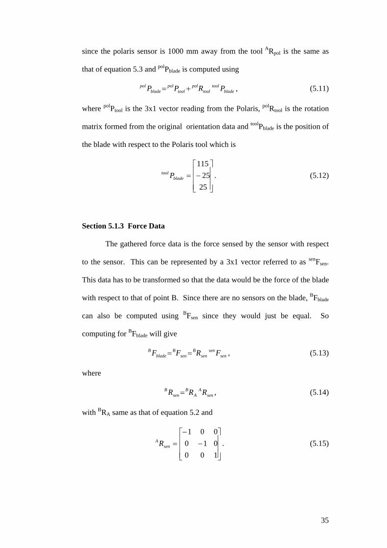
35
since the polaris sensor is 1000 mm away from the tool ARpol is the same as
that of equation 5.3 and polPblade is computed using
bladetool
toolpol
toolpol
bladepol PRPP += , (5.11)
where polPtool is the 3x1 vector reading from the Polaris, polRtool is the rotation
matrix formed from the original orientation data and toolPblade is the position of
the blade with respect to the Polaris tool which is
⎥⎥⎥
⎦
⎤
⎢⎢⎢
⎣
⎡−=2525
115
bladetool P . (5.12)
Section 5.1.3 Force Data
The gathered force data is the force sensed by the sensor with respect
to the sensor. This can be represented by a 3x1 vector referred to as senFsen.
This data has to be transformed so that the data would be the force of the blade
with respect to that of point B. Since there are no sensors on the blade, BFblade
can also be computed using BFsen since they would just be equal. So
computing for BFblade will give
sensen
senB
senB
bladeB FRFF == , (5.13)
where
senA
AB
senB RRR = , (5.14)
with BRA same as that of equation 5.2 and
⎥⎥⎥
⎦
⎤
⎢⎢⎢
⎣
⎡−
−=
100010001
senAR . (5.15)
36
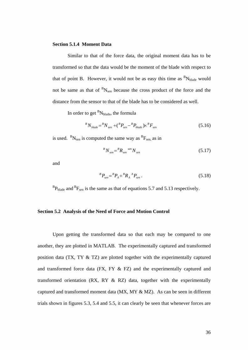
Section 5.1.4 Moment Data
Similar to that of the force data, the original moment data has to be
transformed so that the data would be the moment of the blade with respect to
that of point B. However, it would not be as easy this time as BNblade would
not be same as that of BNsen because the cross product of the force and the
distance from the sensor to that of the blade has to be considered as well.
In order to get BNblade, the formula
senB
bladeB
senB
senB
bladeB FPPNN ×−+= )( (5.16)
is used. BNsen is computed the same way as BFsen, as in
sensen
senB
senB NRN = (5.17)
and
senA
AB
AB
senB PRPP += . (5.18)
BPblade and BFsen is the same as that of equations 5.7 and 5.13 respectively.
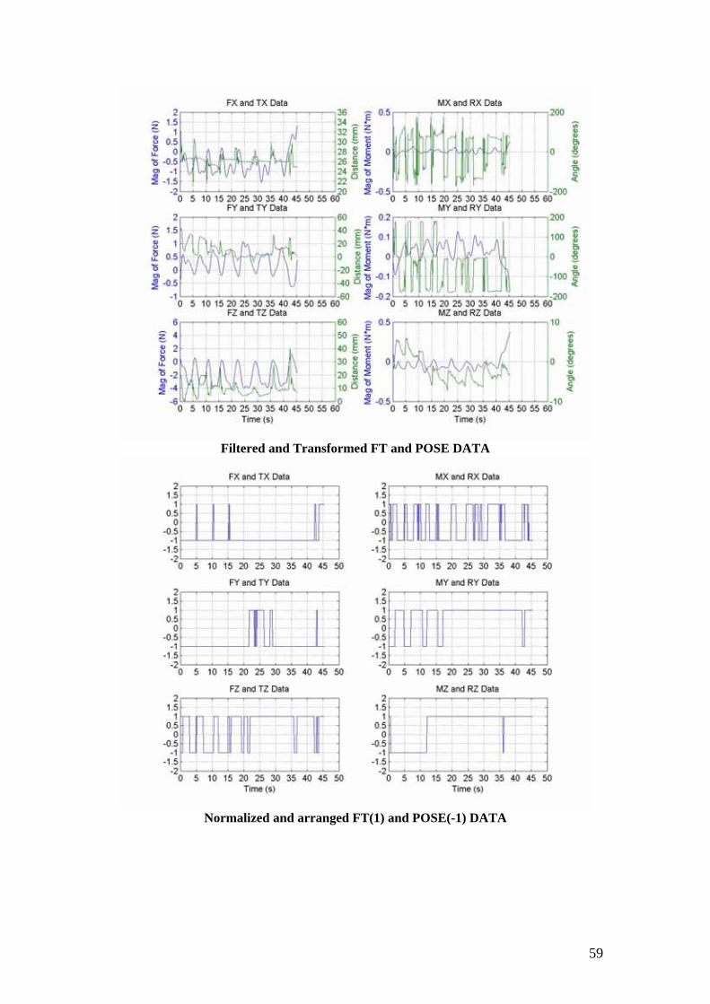
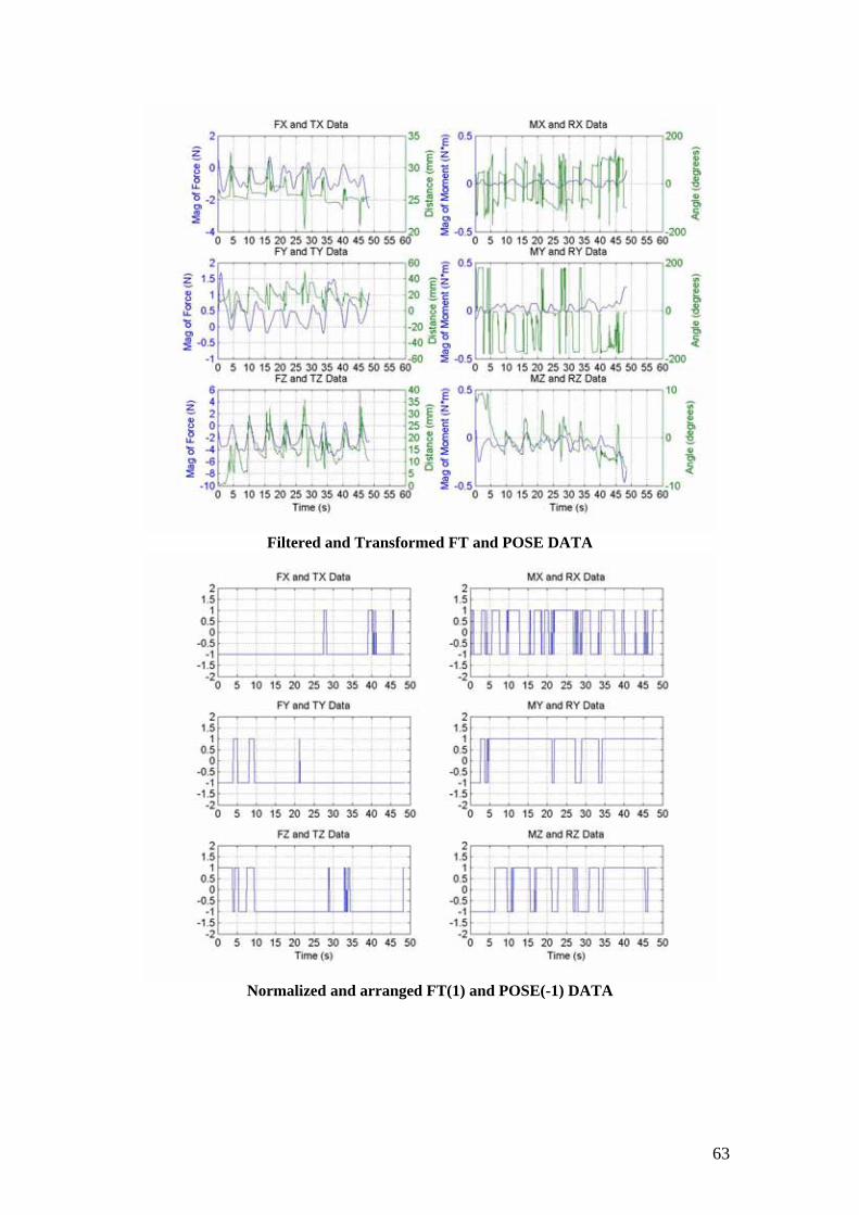
Section 5.2 Analysis of the Need of Force and Motion Control
Upon getting the transformed data so that each may be compared to one
another, they are plotted in MATLAB. The experimentally captured and transformed
position data (TX, TY & TZ) are plotted together with the experimentally captured
and transformed force data (FX, FY & FZ) and the experimentally captured and
transformed orientation (RX, RY & RZ) data, together with the experimentally
captured and transformed moment data (MX, MY & MZ). As can be seen in different
trials shown in figures 5.3, 5.4 and 5.5, it can clearly be seen that whenever forces are

37
applied at a particular axis (ref frame B), relatively low or no motion are done at all
on that axis.
It is also noticeable that the forces along the x and y axis are relatively small
compared to that of the z axis. Taking into consideration the inaccuracy of the point
of contact, it is possible that there is actually minimal or no force applied at all on the
x and y axis.
Another noticeable aspect is that rotations about the x and y axes are abundant
compared to rotation about the z axis. Taking to account the instability and
inefficiency of a human worker, it is possible that there would be no rotation about the
z axis at all. More of these graphs are shown in Appendix B and C.
Figure 5.3 Graph of FT and POSE data (Trial 1)

38
Figure 5.4 Graph of FT and POSE data (Trial 2)
Figure 5.5 Graph of FT and POSE data (Trial 3)
39
CHAPTER 6 Recommendations for Compliant Motion Required
for Polishing
In order to achieve compliant motion in polishing, it is clear that both force
and motion control is needed. It is the question of when force control and motion
control are needed and how much force and or motion are needed as well. This
chapter discusses the recommended guidelines for polishing a turbine blade based on
the data gathered and analyzed.
Section 6.1 Amount of Force and Motion Needed
Based on the data analysis done on Chapter 5, it can be seen that the most
dominant force factor is the force along the z-axis or the axis normal to the point of
contact between the polisher and the workpiece. From the data gathered (filtered and
transposed force and torque readings), a force of around 4 to 5 Newtons is applied
along the normal axis. It can also be seen that the length of time this force applied by
the worker is averaging somewhere around 4 seconds. A force of around 1 Newton
occasionally applied to the x and y-axis was noticed as well, but this can be attributed
to the inaccuracy of the assumed or estimated point of contact. The same force
behavior was observed for both concave and convex side of the blade.
For the convex side of the blade, the motion along the x, y and z axis are
mainly due to the times when the workpiece is checked by the worker. The distances

40
of these motions are not really significant as long as they are far enough from the
polisher for checking - in this case, a distance of around 30 to 50 millimeters. It can
probably be said that having a constant position is better and safer because from
experience, translational motion of the blade can result in some slippage and
accidents. If ever translational motion would be needed, the motion of the blade
should be opposite to that of the direction of the belt sander.
With regards to rotation, the motion about the z-axis is relatively small
compared to that of the x and y axes. Rotations of around ±150 degrees were
observed in the x-axis and around ±190 for the y-axis. These rotational motions are to
needed to follow the curved shape of the blade. The more curved the blade is, the
more rotations would be needed. Without these rotations only the middle part of the
blade would be polished. Rotations of around ± 10 degrees were observed in the z
axis which can be attributed to the instability of the human hand.
Unlike polishing the convex side of the blade, polishing the concave needs
less rotation (as can be seen in Appendix B and C). This is because the curved shape
of the blade now matches with the curve of the roller of the belt sander. However this
still depends on the size or diameter of the rollers and the concavity of the blade.
Small rollers and broader concavity would mean more rotation and even some
translation along x and y axes. Using big rollers with a narrower concavity might not
be able to do the polishing well as there might be some points where the belt sander
would not reach the inner part of the concave blade.

41
In the case of the moments, an average value of around 0.1 Newton-meters
were observed in all the axes.
Section 6.2 When to Use Force and Motion Control
It is already understood that both force and motion control is needed for the
automation of the polishing process. After analyzing the amount of force to be
applied and the motions to be done, the time to use these values are now discussed.
It should be clear by now that when force control is being used, there would be
no motion control. It can clearly be seen from the graphs of figures 5.1, 5.2 and 5.3
that there were no movements when force was applied. Similarly, when there were
movements, no force was detected.
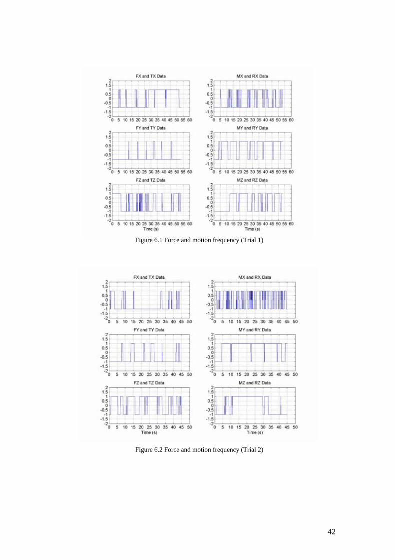
In order to know when force control and motion control should be used, the
data from Chapter 5 was normalized and compared. Figures 6.1 to 6.3 shows a chart
when motion is more important than force (thus motion control is required) and vise
versa. In the graph, a value of positive one denotes force control and negative one
represents motion control. Based on the graph of the 13 trials (seen in Appendix B
and C), the alternation between force and motion control is somewhere at the
frequency of 0.2 to 0.5 Hz.
42
Figure 6.1 Force and motion frequency (Trial 1)
Figure 6.2 Force and motion frequency (Trial 2)

43
Figure 6.3 Force and motion frequency (Trial 3)

44
CHAPTER 7 Conclusion
Experiments were done to study the motion and forces required to do the task
of polishing turbine blades. To do this, turbine polishings were done using a small
polisher with a force-torque sensor attached to record FT readings and the blade being
polished was attached to the Polaris to record POSE readings.
Upon analysis and investigation of the parameters involved in the polishing of
a turbine blade, it was learned there are actually fewer important parameters than were
expected. From the data gathered, it shows that only the force along the z-axis
(normal to the polisher) and the rotations about the x and y axes have very significant
values during polishing. Other motions were also recorded but they were from the
motions when the worker checks on the workpiece, which is not really part of the
main polishing process.
With this work, automating the turbine polishing process becomes less
difficult because one would know which parameters to concentrate on. Presented in
chapter 6 are recommended data that can be used in automation of the polishing
process such as when to use force and motion control and some specific values for
force and motion.
Nevertheless, rooms for further research on this topic are still very open.
Improvements in the setup of the experiment can still be done. Using a better polisher

45
would be able to give better results since this could eliminate the much unwanted
noise that affected the FT readings.

46
REFERENCES
F. Nagata, K. Watanabe, Polishing Robot with Human Friendly Joystick Teaching System, Human friendly mechatronics: selected papers of the International Conference on Machine Automation: ICMA2000, September 27-29, 2000, Osaka, Japan pp. 327-332.
F. Nagata, K. Watanabe, Teaching System for a Polishing Robot using a Game
Joystick, SICE 2000: proceedings of the 39th SICE Annual Conference: international session papers: Iizuka, Japan, 26-28 July, 2000 pp 179-184.
J. Rosell, J. Gratacos, L. Basanez, An Automatic Programming Tool for Robotic
Polishing Tasks, Proceedings of the 1999 IEEE International Symposium on Assembly and Task Planning (ISATP '99): towards flexible and agile assembly and manufacturing: July 21-24, 1999, Porto, Portugal pp 250-255.
X. D. Zhang, W. Wang, Setpoints Optimization and Predictive Control for Grinding
Process, Low cost automation 1998: (LCA'98): a proceedings volume from the 5th IFAC Symposium, Shenyang, P.R. China, 8-10 September 1998 pp. 163-168.
B. W. Kruszynski, S. Midera, Forces in Gear Grinding - Theoretical and
Experimental Approach, Advanced manufacturing systems and technology, Wien; New York: Springer, 1996. Pp 201-208.
A. Ananiev, Robotics usage for belt-grinding for parts with complicated shapes,
Mechatronics - the basis for new industrial development, Southampton; Boston: Computational Mechanics Publications, c1994 Pp. 141-146
A. Ikonomopoulos, L. Dritsas, Recent Advances in Robot Grinding, Robotic systems:
advanced techniques and applications, Dordrecht; Boston: Kluwer Academic, c1992 pp 603 – 610.
L.E. Samuels, Metallographic polishing by mechanical methods, Imprint Materials
Park, OH: ASM International, c2003. 4th ed. X. Chen, R. Devanathan, A. M. Fong, Advanced automation techniques in adaptive
material processing, Singapore: World Scientific, c2002. Xipeng Xu, Jianyun Shen, Yuan Li, Conference Grinding and Machining Conference,
(11th : 2001 : Quanzhou, China), Title Advances in abrasive processes: selected papers from the 11th Grinding and Machining Conference, June 2-6,

47
2001, Quanzhou, China, Imprint Uetikon-Zuerich, Switzerland : Trans Tech Publications Ltd, c2001.
G. Petzow, Metallographisches Ätz (Metallographic etching), techniques for
metallotraphy, ceramography, plastography, in collaboration with Veronika Carle translated by Uta Hanisch, Imprint Materials Park, OH: ASM International, c1999. 2nd ed.
L.K. Gillespie, Deburring and edge finishing handbook, Imprint Dearborn, Mich.:
Society of Manufacturing Engineers; New York: American Society of Mechanical Engineers, c1999.
J. Brown, Advanced machining technology handbook, Imprint New York: McGraw-
Hill, c1998. D. Frisch, S. Frisch, Metal: design and fabrication, photography by Joshua White,
Imprint New York: Whitney Library of Design, c1998. M.C. Shaw, Principles of abrasive processing, Imprint Oxford: Clarendon Press; New
York: Oxford University Press, c1996. G.P. Shpenkov, Friction surface phenomena, Imprint Amsterdam; New York:
Elsevier, c1995. S.C. Salmon, Modern grinding process technology, Imprint New York: McGraw-Hill,
c1992. S. Malkin, Grinding technology: theory and applications of machining with abrasives,
Imprint New York: Halsted Press, c1989. R.I. King, R.S. Hahn, Handbook of modern grinding technology, Imprint New York:
Chapman and Hall, c1986. C. Andrew, T.D. Howes, T.R.A. Pearce, Creep feed grinding, Imprint London: Holt,
Rinehart and Winston, c1985. M.C. Shaw, Milton C. Shaw Grinding Symposium, sponsored by the Production
Engineering Division, presented at the Winter Annual Meeting of the American Society of Mechanical Engineers, November 17-22, 1985, Miami Beach, Florida; edited by R. Komanduri, D. Maas, Imprint New York: ASME, c1985.
R.L. McKee, Machining with abrasives, Imprint New York: Van Nostrand Reinhold,
c1982. L.E. Samuels, Metallographic polishing by mechanical methods, Imprint Metals Park,
Ohio: American Society for Metals, c1982. 3rd ed.

48
D.L. Brown, Grinding dynamics, Imprint Cincinnati, Ohio: University of Cincinnatti, c1976.
T. M. Stephien, L. M. Sweet, M. C. Good, M. Tomizuka, Control of Tool/ Workpiece
Contact Force with Application to Robotic Deburring, IEEE Journal of Robotics and Automation,Vol. RA-3, No. 1, February 1987, pp. 7 -18
S. S. Ge, X. Q. Chen, S. Xie and D. L. Gu, Coordinated Motion and Force Control of
a Cartesian Arm and A Rotary Table, Proceedings of the IEEE Singapore International Symposium on Control Theory and Applications, July 20-30, 1997, pp.180-289.
T. Engel, R. Tomastik, Description of the Chamfering and Deburring End-Of-Arm
Tool (CADET), The Fourth International Conference on Control, Automation, Robotics and Vision, December 2-6, 1996, Singapore, pp. 629 – 633.
U. Berger, R. Janssen, E. Brinksmeier, Advanced Mechatronic System for Turbine
Blade Manufacturing and Repair, International Conference on Computer Integrated Manufacturing, 1997, Singapore.
M. Kunieda, T. Nakagawa, Robot-Polishing of Curved Surface with Magneto-Pressed
Tool and Magnetic Force Sensor, Proceedings of 25th International MTDR Conference, April 1985, pp. 193-200.
F. Ozaki, M. Jinno, T. Yoshimi, K. Tatsuno, M. Takahashi, M. Kanda, Y. Tamada and
S. Nagataki, A Force Controlled Finishing Robot System with a Task-Directed Robot Language, Journal of Robotics and Mechatronics, Vol. 7, No. 5, c1995, p.383.
M. Jinno, F. Ozaki, T. Yoshida, K. Tatsuno, Development of a Force Controlled
Robot for Grinding, Chamfering and Polishing, Proceedings of the IEEE International Conference on Robotics and Automation, 1995, p.1455
F. Pfeiffer, H. Bremer, J. Figueiredo, Surface Polishing with Flexible Link
Manipulators, European Journal of Mechanics, A/Solids, Vol. 15, No. 1, c1996, p.137.
F. Nagata, K. Watanabe, An Experiment on Sanding Task Using Impedance
Controlled Manipulator with Vibrational Type Tool, Proceedings of the Third Asian Control Conference, 2000, p.2989.
F. Nagata, K. Watanabe, K. Izumi, An Experiment on Profiling Task with Impedance
Controlled Manipulator Using Cutter Location Data, Proceedings of the IEEE International Conference on System, Man and Cybernetics (SMC'99), 1999, p.848.
F. Nagata, K. Watanabe, K. Izumi, Profiling Control for Industrial Robots Using a
Position Compensator Based on Cutter Location Data, Journal of the Japan Society for Precision Engineering, Vol. 66, No. 3, c2000, p.473 (in Japanese).

49
K. Takahashi, S. Aoyagi, M. Takano, Study on a Fast Profiling Task of a Robot with Force Control Using Feedforward of Predicted Contact Position Data, Proceedings of the 4th Japan-France Congress & 2nd Asia-Europe Congress on Mechatronics, Vol. 1, c1998, p.398.
DSP-Based Force Sensor Receivers Software and installation manual, Nitta
Corporation, Nov. 1994. Polaris Optical Tracking System Application Programmer’s Interface Guide Manual
version 1.0, Northern Digital Inc., April 1999. Polaris Optical Tracking system Instruction Manual Version 1.1, October 2000 Signal processing toolbox users’ guide version 4, MATLAB

50
APPENDIX A
TRANSFORMATION COMPUTATIONS

51
⎥⎥⎥
⎦
⎤
⎢⎢⎢
⎣
⎡=
00
1000
polAP
⎥⎥⎥
⎦
⎤
⎢⎢⎢
⎣
⎡
+−=
)cos(325325)sin(325
0
2
2
QQPA
B ⎥⎥⎥
⎦
⎤
⎢⎢⎢
⎣
⎡−=
9.90050
senAP
⎥⎥⎥
⎦
⎤
⎢⎢⎢
⎣
⎡=
z
y
x
toolpol
TTT
P ⎥⎥⎥
⎦
⎤
⎢⎢⎢
⎣
⎡−=2525
115
bladetool P
⎥⎥⎥
⎦
⎤
⎢⎢⎢
⎣
⎡−=
)cos()sin(0)sin()cos(0
001
22
22
QQQQRA
B
⎥⎥⎥
⎦
⎤
⎢⎢⎢
⎣
⎡
−−=
010001100
polAR
⎥⎥⎥
⎦
⎤
⎢⎢⎢
⎣
⎡−
−=
)cos()sin(0)sin()cos(0
001
11
11
QQQQRblade
tool
⎥⎥⎥
⎦
⎤
⎢⎢⎢
⎣
⎡=
333231
232221
131211
RRRRRRRRR
Rtoolpol
⎥⎥⎥
⎦
⎤
⎢⎢⎢
⎣
⎡−=
000010001
senAR
)cos()cos()sin()cos(
)sin()sin()cos()cos()sin()sin()cos()cos()sin()sin()sin(
)cos()sin()sin()sin()cos()sin()cos()cos()sin()sin()sin()cos(
)cos()cos(
33
32
31
23
22
21
13
12
11
RXRYRRXRYR
RYRRXRZRXRYRZRRXRZRXRYRZR
RYRZRRXRZRXRYRZRRXRZRXRYRZR
RYRZR
==−=
−=+=
=+=−=
=
bladetool
toolpol
polA
AB
bladeB RRRRR =
⎥⎥⎥
⎦
⎤
⎢⎢⎢
⎣
⎡−
−
⎥⎥⎥
⎦
⎤
⎢⎢⎢
⎣
⎡
⎥⎥⎥
⎦
⎤
⎢⎢⎢
⎣
⎡
−−
⎥⎥⎥
⎦
⎤
⎢⎢⎢
⎣
⎡−=
)cos()sin(0)sin()cos(0
001
010001100
)cos()sin(0)sin()cos(0
001
11
11
333231
232221
131211
22
22
QQQQ
RRRRRRRRR
QQQQ
⎥⎥⎥
⎦
⎤
⎢⎢⎢
⎣
⎡
++−−++−−++−−
⎥⎥⎥
⎦
⎤
⎢⎢⎢
⎣
⎡
−−
⎥⎥⎥
⎦
⎤
⎢⎢⎢
⎣
⎡−=
)cos()sin()sin()cos()cos()sin()sin()cos()cos()sin()sin()cos(
010001100
)cos()sin(0)sin()cos(0
001
13313213313231
12312212312221
11311211311211
22
22
QRQRQRQRRQRQRQRQRRQRQRQRQRR
QQQQ
⎥⎥⎥
⎦
⎤
⎢⎢⎢
⎣
⎡
−−−−−−++−−
⎥⎥⎥
⎦
⎤
⎢⎢⎢
⎣
⎡−=
)cos()sin()sin()cos()cos()sin()sin()cos(
)cos()sin()sin()cos(
)cos()sin(0)sin()cos(0
001
12112212312221
11311211311211
13313213313231
22
22
QRQRQRQRRQRQRQRQRR
QRQRQRQRR
QQQQ

52
)cos(*.)sin(*.)sin(*.)cos(*.
)cos(*.)sin(*.)sin(*.)cos(*.
)cos(*.)sin(*.)sin(*.)cos(*.
12312233
12312232
2131
11311223
11311222
1121
13313213
13313212
3111
QRQRnRQRQRnR
RnRQRQRnR
QRQRnRRnR
QRQRnRQRQRnR
RnR
−−=+=
=−−=−=
=+=+−=
−=
⎥⎥⎥
⎦
⎤
⎢⎢⎢
⎣
⎡
−+−−+−−+−−+−−−−−−−=
)cos(*.)sin(*.)cos(*.)sin(*.)cos(*.)sin(*.)sin(*.)cos(*.)sin(*.)cos(*.)sin(*.)cos(*.
233223232222231221
233223232222231221
131211
QnRQnRQnRQnRQnRQnRQnRQnRQnRQnRQnRQnR
nRnRnRRblade
B
bladeA
AB
AB
bladeB PRPP +=
bladepol
polA
polA
bladeA PRPP +=
bladetool
toolpol
toolpol
bladepol PRPP +=
⎥⎥⎥
⎦
⎤
⎢⎢⎢
⎣
⎡=
1
1
1
TzTyTx
Pbladepol
⎥⎥⎥
⎦
⎤
⎢⎢⎢
⎣
⎡=
2
2
2
TzTyTx
PbladeA
⎥⎥⎥
⎦
⎤
⎢⎢⎢
⎣
⎡=
newTznewTynewTx
PbladeB
⎥⎥⎥
⎦
⎤
⎢⎢⎢
⎣
⎡
+−+−+−
+⎥⎥⎥
⎦
⎤
⎢⎢⎢
⎣
⎡=
⎥⎥⎥
⎦
⎤
⎢⎢⎢
⎣
⎡−
⎥⎥⎥
⎦
⎤
⎢⎢⎢
⎣
⎡
+⎥⎥⎥
⎦
⎤
⎢⎢⎢
⎣
⎡=
⎥⎥⎥
⎦
⎤
⎢⎢⎢
⎣
⎡=
333231
232221
131211
333231
232221
131211
1
1
1
252511525251152525115
2525
115
RRRRRRRRR
TzTyTx
RRR
RRR
RRR
TzTyTx
TzTyTx
Pbladepol
⎥⎥⎥
⎦
⎤
⎢⎢⎢
⎣
⎡
∗+∗−∗+∗+∗−∗+∗+∗−∗+
=⎥⎥⎥
⎦
⎤
⎢⎢⎢
⎣
⎡
25332532115312523252211521
2513251211511
1
1
1
RRRTzRRRTy
RRRTx
TzTyTx
⎥⎥⎥
⎦
⎤
⎢⎢⎢
⎣
⎡=
⎥⎥⎥
⎦
⎤
⎢⎢⎢
⎣
⎡
−−
+=
⎥⎥⎥
⎦
⎤
⎢⎢⎢
⎣
⎡
−−+
⎥⎥⎥
⎦
⎤
⎢⎢⎢
⎣
⎡=
⎥⎥⎥
⎦
⎤
⎢⎢⎢
⎣
⎡
⎥⎥⎥
⎦
⎤
⎢⎢⎢
⎣
⎡
−−+
⎥⎥⎥
⎦
⎤
⎢⎢⎢
⎣
⎡=
2
2
2
1
1
1
1
1
1
1
1
1 1000
00
1000
010001100
00
1000
TzTyTx
TyTx
Tz
TyTxTz
TzTyTx
PbladeA

53
⎥⎥⎥
⎦
⎤
⎢⎢⎢
⎣
⎡
⎥⎥⎥
⎦
⎤
⎢⎢⎢
⎣
⎡
−−−+
⎥⎥⎥
⎦
⎤
⎢⎢⎢
⎣
⎡
+−=
2
2
2
22
22
2
2
)cos()sin(0)sin()cos(0
001
)cos(5.325.32)sin(5.32
0
TzTyTx
QQQQ
QQPblade
B
⎥⎥⎥
⎦
⎤
⎢⎢⎢
⎣
⎡
−+−−−+
⎥⎥⎥
⎦
⎤
⎢⎢⎢
⎣
⎡
+−=
)cos()sin()sin()cos(
)cos(5.325.32)sin(5.32
0
2222
2222
2
2
2
QTzQTyQTzTyQ
Tx
⎥⎥⎥
⎦
⎤
⎢⎢⎢
⎣
⎡
−∗+−∗+∗+−−∗−−∗+∗=
⎥⎥⎥
⎦
⎤
⎢⎢⎢
⎣
⎡=
)cos()sin()cos(5.325.32)sin()cos()sin(5.32
22222
22222
2
QTzQTyQQTzQTyQ
Tx
newTznewTynewTx
PbladeB
blade
Bsen
sensen
AA
Bsen
sensen
Bsen
B PFRRFRF ===
⎥⎥⎥
⎦
⎤
⎢⎢⎢
⎣
⎡
⎥⎥⎥
⎦
⎤
⎢⎢⎢
⎣
⎡−
−
⎥⎥⎥
⎦
⎤
⎢⎢⎢
⎣
⎡
−−−−=
FzFyFx
QQQQ
100010001
cos)sin(0)sin()cos(0
001
22
22
⎥⎥⎥
⎦
⎤
⎢⎢⎢
⎣
⎡
−∗+−∗−−∗−−∗−
−=
⎥⎥⎥
⎦
⎤
⎢⎢⎢
⎣
⎡
⎥⎥⎥
⎦
⎤
⎢⎢⎢
⎣
⎡
−−−−−−−
−=
)cos()sin()sin()cos(
)cos()sin(0)sin()cos(0
001
22
22
22
22
QFzQFyQFzQFy
Fx
FzFyFx
QQQQ
⎥⎥⎥
⎦
⎤
⎢⎢⎢
⎣
⎡
−∗+−∗−−∗−−∗−
−=
)cos()sin()sin()cos(
22
22
QMzQMyQMzQMy
MxN sen
B
senB
bladeB
senB
senB
bladeB FPPNN ×−+= )(
( ) senB
bladeB
senA
AB
AB
senB FPPRPN ×−++=
senB
senB F
newTznewTynewTx
QQQQ
QQN ×
⎟⎟⎟
⎠
⎞
⎜⎜⎜
⎝
⎛
⎥⎥⎥
⎦
⎤
⎢⎢⎢
⎣
⎡−
⎥⎥⎥
⎦
⎤
⎢⎢⎢
⎣
⎡
−
−
⎥⎥⎥
⎦
⎤
⎢⎢⎢
⎣
⎡−+
⎥⎥⎥
⎦
⎤
⎢⎢⎢
⎣
⎡
+−+=
9.900
50
)cos()sin(0)sin()cos(0
001
)cos(5.325.32)sin(5.32
0
22
22
2
2
=⎥⎥⎥
⎦
⎤
⎢⎢⎢
⎣
⎡×⎥⎥⎥
⎦
⎤
⎢⎢⎢
⎣
⎡+
newFznewFynewFx
zTempyTempxTemp
NsenB ,where
⎥⎥⎥
⎦
⎤
⎢⎢⎢
⎣
⎡
−−+−−+
−
⎥⎥⎥
⎦
⎤
⎢⎢⎢
⎣
⎡
)cos(9.90)cos(5.325.32)sin(9.90)sin(5.32
50
22
22
QQQQ
zTempyTempxTemp

54
=⎥⎥⎥
⎦
⎤
⎢⎢⎢
⎣
⎡
−−−
+newFxyTempnewFyxTempnewFzxTempnewFxzTempnewFyzTempnewFzyTemp
N senB

55
APPENDIX B
GRAPHS OF CONVEX DATA
56
TRIAL 1
Frequency analysis of FT DATA and NOISE DATA
Filtered and unfiltered FT DATA

57
Filtered and Transformed FT and POSE DATA
Normalized and arranged FT(1) and POSE(-1) DATA

58
TRIAL 2
Frequency analysis of FT DATA and NOISE DATA
Filtered and unfiltered FT DATA
59
Filtered and Transformed FT and POSE DATA
Normalized and arranged FT(1) and POSE(-1) DATA

60
TRIAL 3
Frequency analysis of FT DATA and NOISE DATA
Filtered and unfiltered FT DATA

61
Filtered and Transformed FT and POSE DATA
Normalized and arranged FT(1) and POSE(-1) DATA

62
TRIAL 4
Frequency analysis of FT DATA and NOISE DATA
Filtered and unfiltered FT DATA
63
Filtered and Transformed FT and POSE DATA
Normalized and arranged FT(1) and POSE(-1) DATA

64
TRIAL 5
Frequency analysis of FT DATA and NOISE DATA
Filtered and unfiltered FT DATA

65
Filtered and Transformed FT and POSE DATA
Normalized and arranged FT(1) and POSE(-1) DATA

66
TRIAL 6
Frequency analysis of FT DATA and NOISE DATA
Filtered and unfiltered FT DATA

67
Filtered and Transformed FT and POSE DATA
Normalized and arranged FT(1) and POSE(-1) DATA

68
TRIAL 7
Frequency analysis of FT DATA and NOISE DATA
Filtered and unfiltered FT DATA

69
Filtered and Transformed FT and POSE DATA
Normalized and arranged FT(1) and POSE(-1) DATA
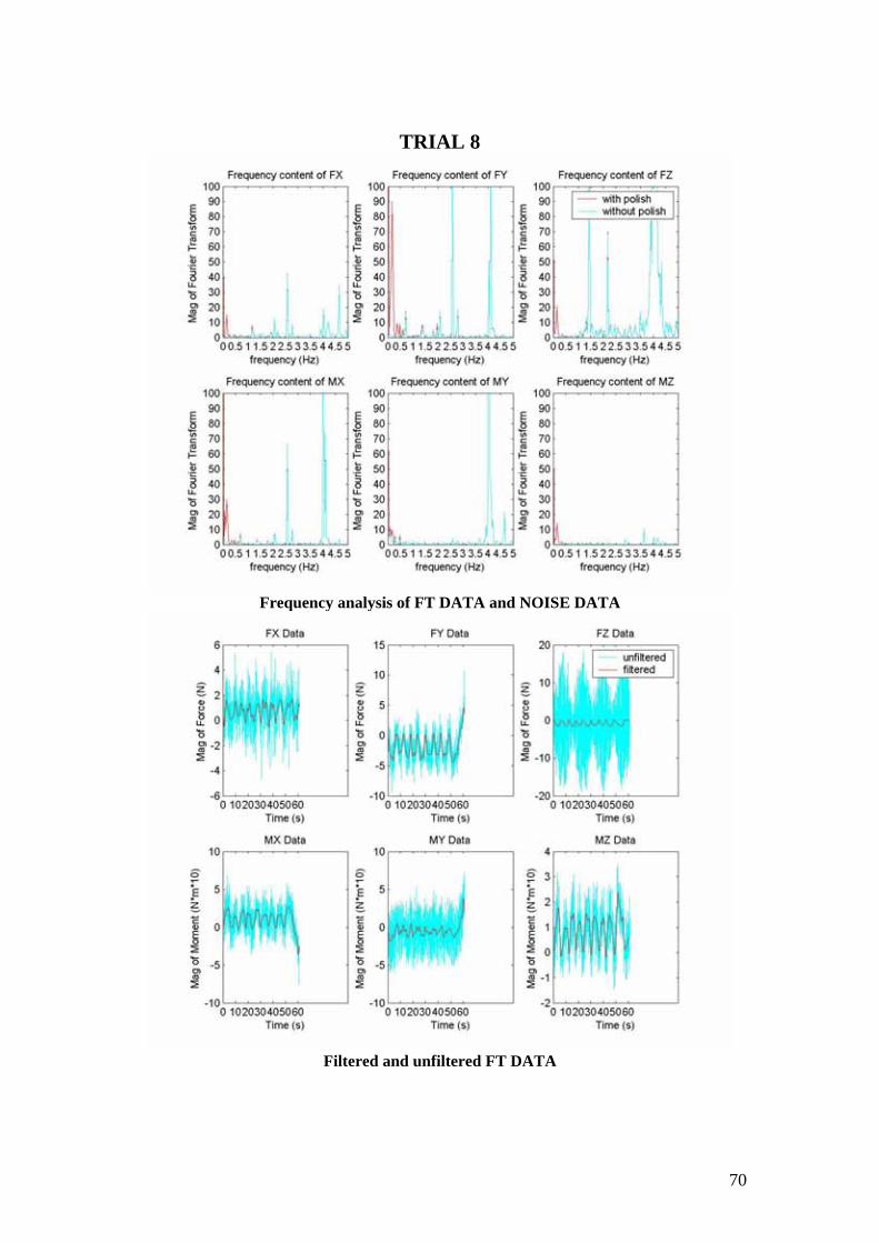
70
TRIAL 8
Frequency analysis of FT DATA and NOISE DATA
Filtered and unfiltered FT DATA

71
Filtered and Transformed FT and POSE DATA
Normalized and arranged FT(1) and POSE(-1) DATA
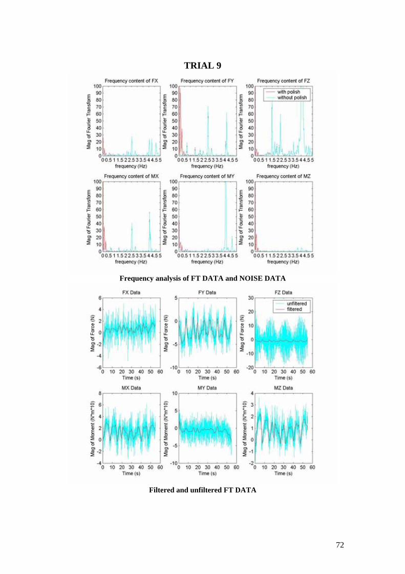
72
TRIAL 9
Frequency analysis of FT DATA and NOISE DATA
Filtered and unfiltered FT DATA
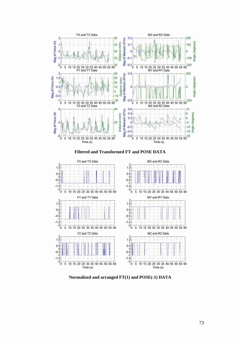
73
Filtered and Transformed FT and POSE DATA
Normalized and arranged FT(1) and POSE(-1) DATA

74
TRIAL 10
Frequency analysis of FT DATA and NOISE DATA
Filtered and unfiltered FT DATA

75
Filtered and Transformed FT and POSE DATA
Normalized and arranged FT(1) and POSE(-1) DATA
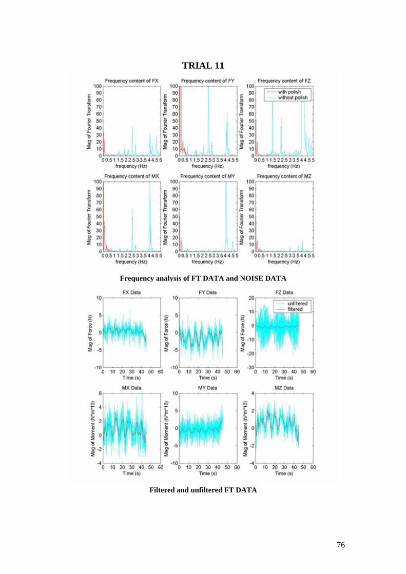
76
TRIAL 11
Frequency analysis of FT DATA and NOISE DATA
Filtered and unfiltered FT DATA

77
Filtered and Transformed FT and POSE DATA
Normalized and arranged FT(1) and POSE(-1) DATA

78
TRIAL 12
Frequency analysis of FT DATA and NOISE DATA
Filtered and unfiltered FT DATA
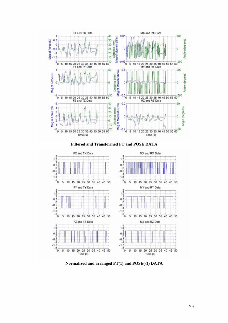
79
Filtered and Transformed FT and POSE DATA
Normalized and arranged FT(1) and POSE(-1) DATA
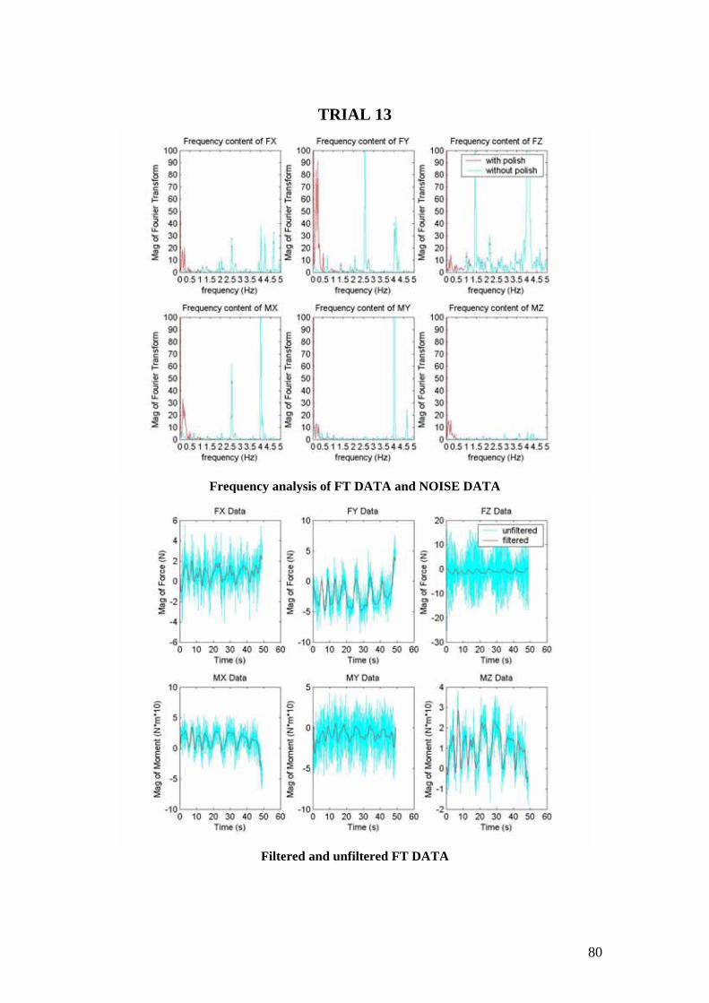
80
TRIAL 13
Frequency analysis of FT DATA and NOISE DATA
Filtered and unfiltered FT DATA
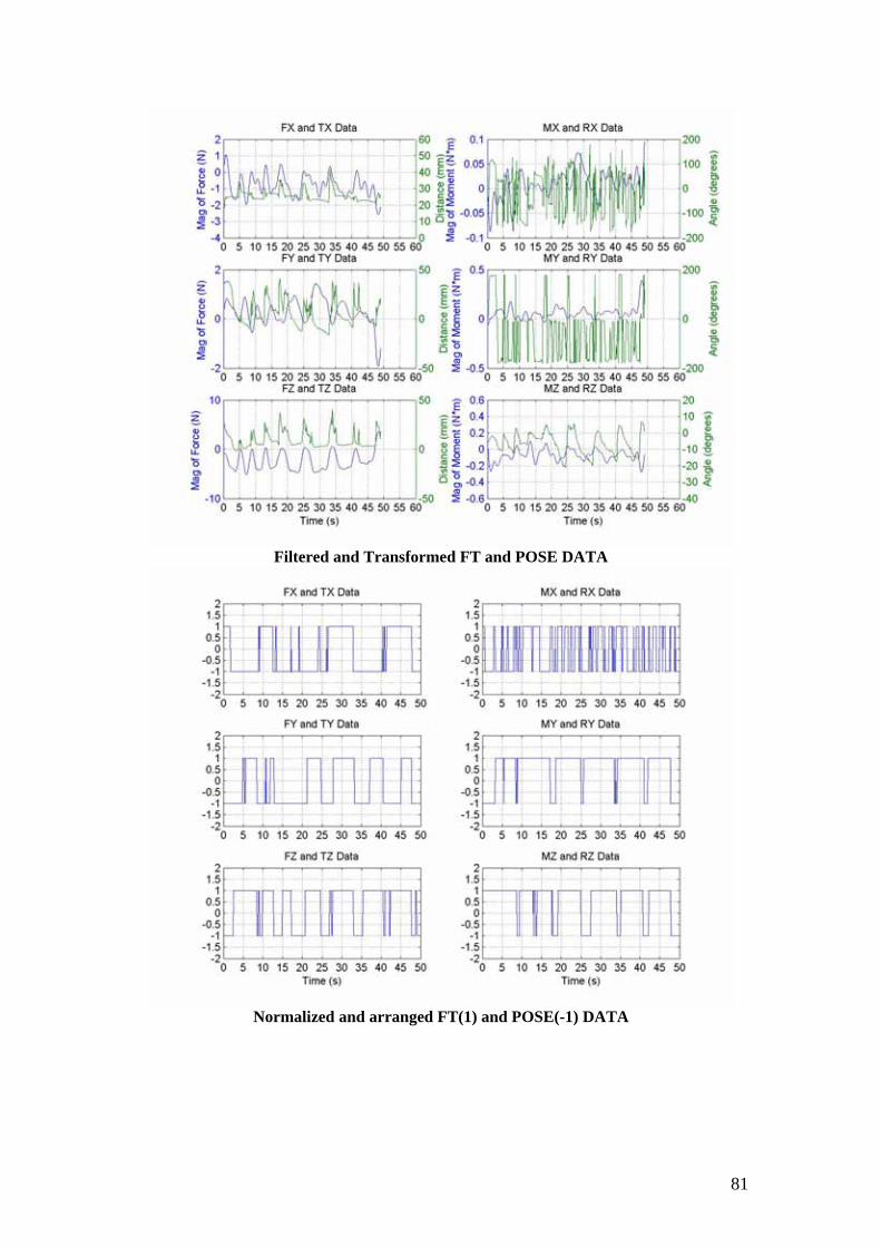
81
Filtered and Transformed FT and POSE DATA
Normalized and arranged FT(1) and POSE(-1) DATA

82
APPENDIX C
GRAPHS OF CONCAVE DATA

83
TRIAL 1
Frequency analysis of FT DATA and NOISE DATA
Filtered and unfiltered FT DATA

84
Filtered and Transformed FT and POSE DATA
Normalized and arranged FT(1) and POSE(-1) DATA

85
TRIAL 2
Frequency analysis of FT DATA and NOISE DATA
Filtered and unfiltered FT DATA
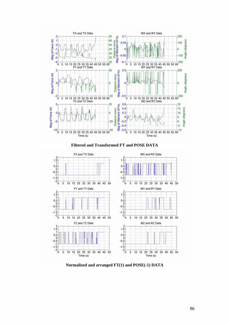
86
Filtered and Transformed FT and POSE DATA
Normalized and arranged FT(1) and POSE(-1) DATA

87
TRIAL 3
Frequency analysis of FT DATA and NOISE DATA
Filtered and unfiltered FT DATA

88
Filtered and Transformed FT and POSE DATA
Normalized and arranged FT(1) and POSE(-1) DATA

89
TRIAL 4
Frequency analysis of FT DATA and NOISE DATA
Filtered and unfiltered FT DATA
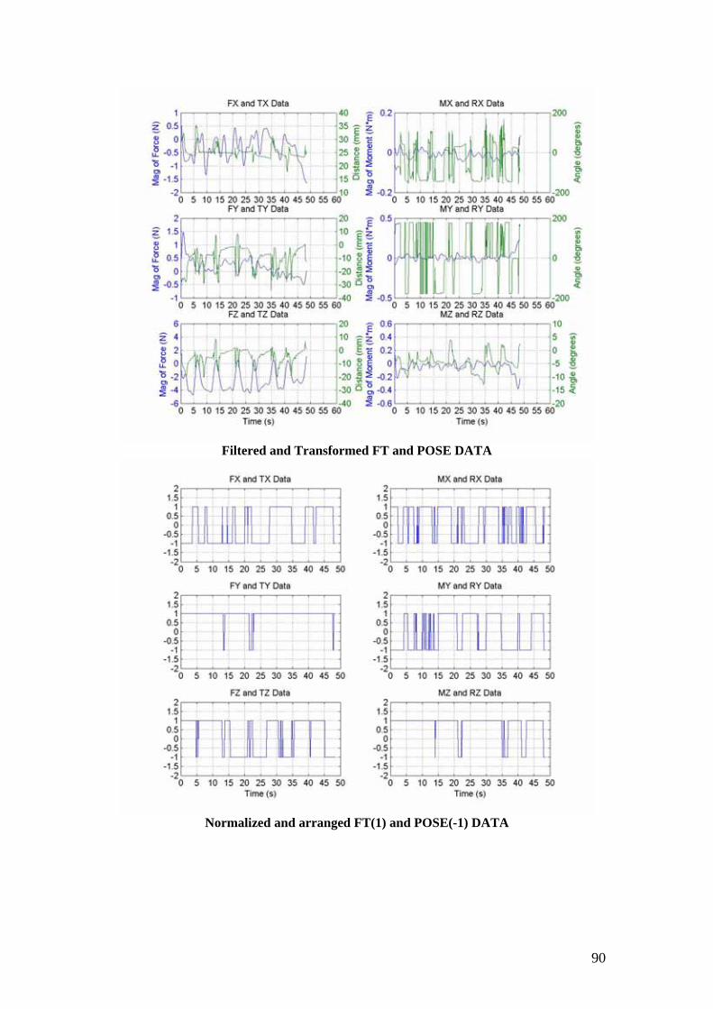
90
Filtered and Transformed FT and POSE DATA
Normalized and arranged FT(1) and POSE(-1) DATA

91
TRIAL 5
Frequency analysis of FT DATA and NOISE DATA
Filtered and unfiltered FT DATA
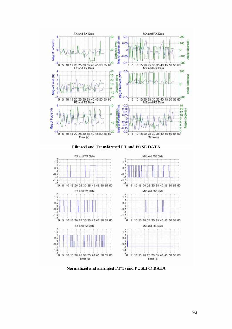
92
Filtered and Transformed FT and POSE DATA
Normalized and arranged FT(1) and POSE(-1) DATA

93
TRIAL 6
Frequency analysis of FT DATA and NOISE DATA
Filtered and unfiltered FT DATA
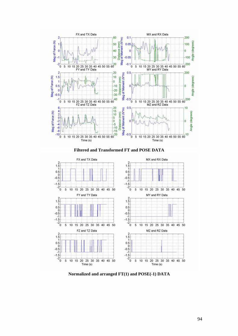
94
Filtered and Transformed FT and POSE DATA
Normalized and arranged FT(1) and POSE(-1) DATA

95
TRIAL 7
Frequency analysis of FT DATA and NOISE DATA
Filtered and unfiltered FT DATA
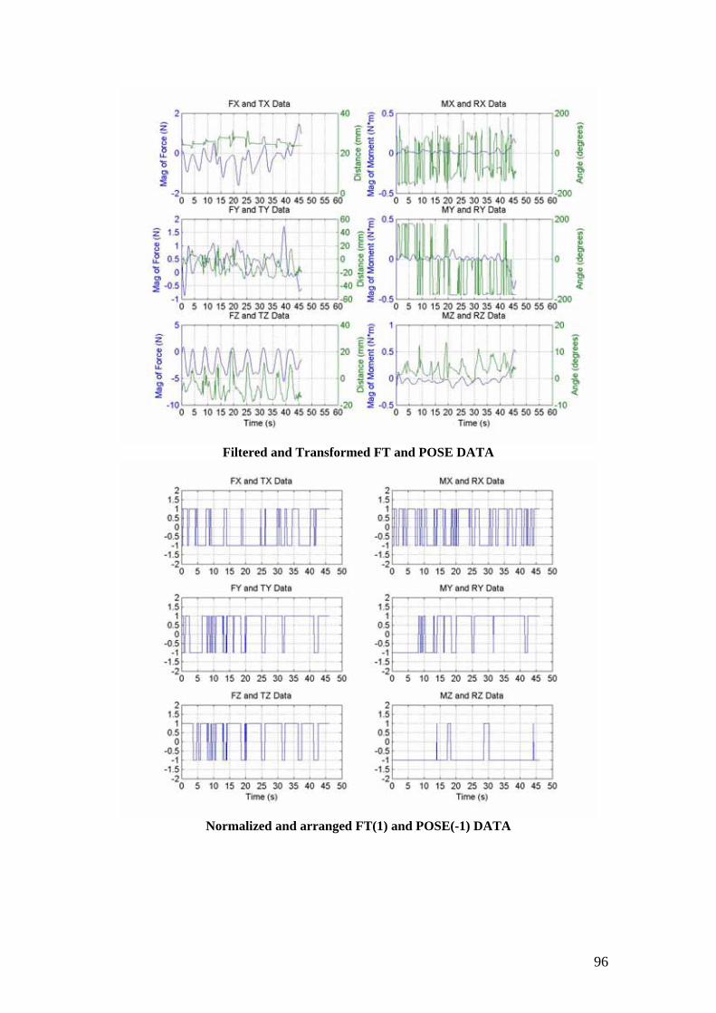
96
Filtered and Transformed FT and POSE DATA
Normalized and arranged FT(1) and POSE(-1) DATA

97
TRIAL 8
Frequency analysis of FT DATA and NOISE DATA
Filtered and unfiltered FT DATA
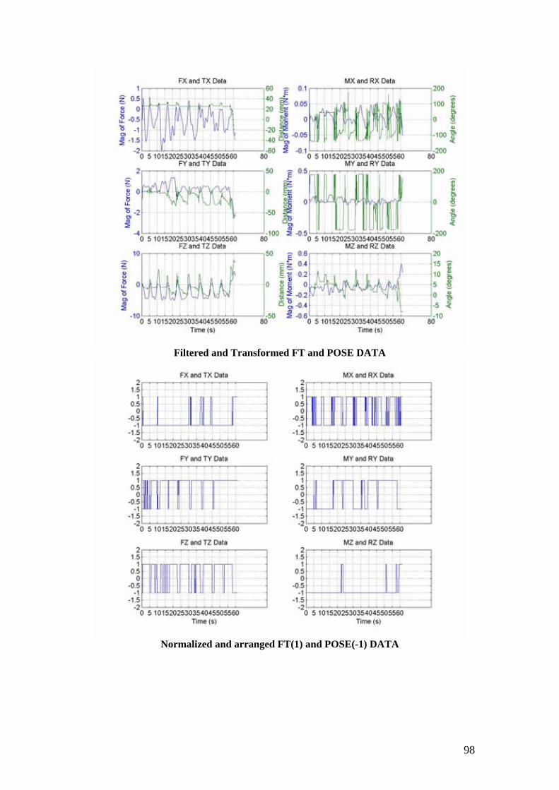
98
Filtered and Transformed FT and POSE DATA
Normalized and arranged FT(1) and POSE(-1) DATA

99
TRIAL 9
Frequency analysis of FT DATA and NOISE DATA
Filtered and unfiltered FT DATA
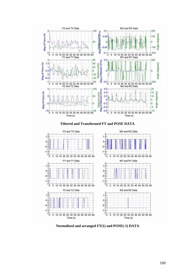
100
Filtered and Transformed FT and POSE DATA
Normalized and arranged FT(1) and POSE(-1) DATA

101
TRIAL 10
Frequency analysis of FT DATA and NOISE DATA
Filtered and unfiltered FT DATA
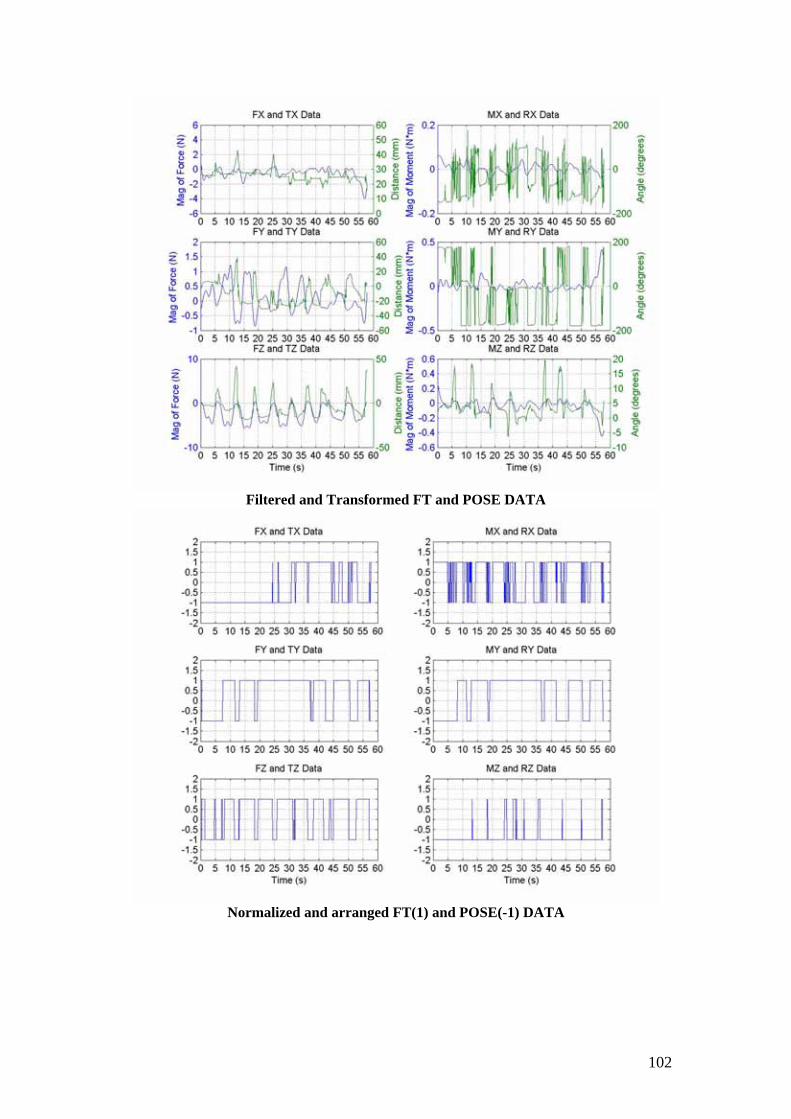
102
Filtered and Transformed FT and POSE DATA
Normalized and arranged FT(1) and POSE(-1) DATA

103
TRIAL 11
Frequency analysis of FT DATA and NOISE DATA
Filtered and unfiltered FT DATA

104
Filtered and Transformed FT and POSE DATA
Normalized and arranged FT(1) and POSE(-1) DATA

105
TRIAL 12
Frequency analysis of FT DATA and NOISE DATA
Filtered and unfiltered FT DATA

106
Filtered and Transformed FT and POSE DATA
Normalized and arranged FT(1) and POSE(-1) DATA

107
TRIAL 13
Frequency analysis of FT DATA and NOISE DATA
Filtered and unfiltered FT DATA

108
Filtered and Transformed FT and POSE DATA
Normalized and arranged FT(1) and POSE(-1) DATA