Markov Chain Monte Carlo: the ultimate multitool - TAPIR Group at

Markov Chain Monte Carlo: the ultimate multitool

Michele Vallisneri, Jet Propulsion Laboratory

Copyright 2013 California Institute of Technology

equal-mass BBH Inspiral: PN equations

merger:numerical relativity

ringdown:perturbation theory

GW science in a nutshell: what’s in a waveform?C

alte

ch/C

orne

ll/C

ITA

NR

equal-mass BBH Inspiral: PN equations

merger:numerical relativity

ringdown:perturbation theory

GW science in a nutshell: what’s in a waveform?C

alte

ch/C

orne

ll/C

ITA

NR

HF GWs: stellar masses LF GWs: massive BHs,large separations

astrophysics populations of compact objects;SN and GRB progenitors*

massive BH origin and evolution; Galactic WD-binary populations and interactions

nuclear physics NS EOS, r-mode processes*

cosmology standard sirens*standard sirens*

fundamental gravity strong-field and radiation-sector dynamicsstrong-field and radiation-sector dynamics

black-hole structure tests of no-hair theoremwith EMRIs, ringdowns

p(source parameters|data) = p(d.|s.p.)× p(s.p.)�p(d.|s.p.)× p(s.p.) d(s.p.)


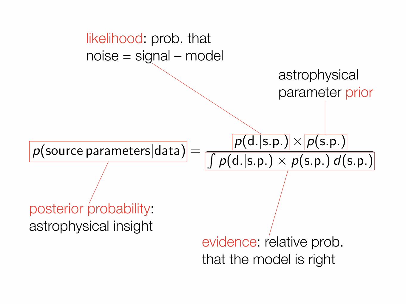
posterior probability:astrophysical insight


likelihood: prob. thatnoise = signal – model





astrophysicalparameter prior




astrophysicalparameter prior

evidence: relative prob.that the model is right

spinning BH–BH injection

spinning NS–BH injection

Monte Carlo (Von Neumann and Ulam, 1946):computational techniques that use random numbers

Monte Carlo (Von Neumann and Ulam, 1946):computational techniques that use random numbers

�φ(x)dx → φ =

1

R

�

r

φ(x (r))

accuracy depends only on variance,not on the number of dimensions

var φ =var φ

R

�φ(x)dx → φ =

1

R

�

r

φ(x (r))

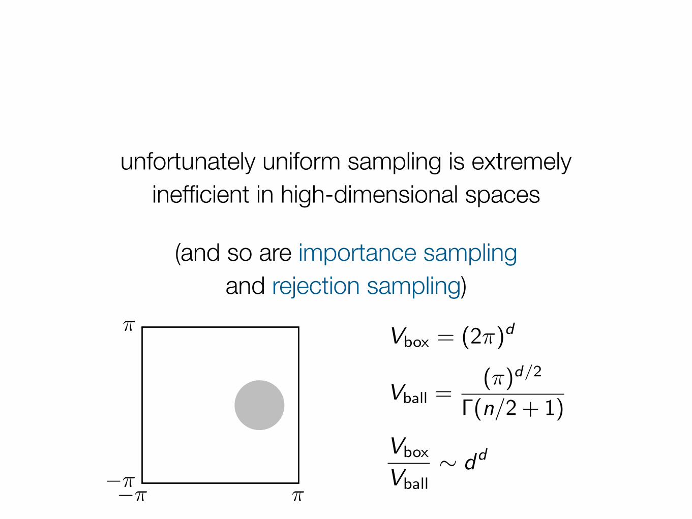
unfortunately uniform sampling is extremelyinefficient in high-dimensional spaces


Vbox = (2π)d

Vball =(π)d/2

Γ(n/2 + 1)

Vbox

Vball∼ dd

π

−ππ−π


Vbox = (2π)d

Vball =(π)d/2

Γ(n/2 + 1)

Vbox

Vball∼ dd

π

−ππ−π

(and so are importance samplingand rejection sampling)

Nicholas Metropolis and hisMathematical Analyzer Numerical Integrator And Calculator

Marshall Rosenbluth and Edward Teller

Teller’s crucial suggestion: ensemble averaging...�

φ(x)p(x)dx , with p(x) � e−E(x)/kT

⇓�φ(x)dp(x) � 1

R

�

R

φ(x (r)) with {x (r)}P

...with samples generated by the “Metropolis” algorithm

• given x(r), propose x(r+1) by random walk• accept it if ΔE = E(x(r+1)) – E(x(r)) < 0,

or with probability e–ΔE/kT if ΔE > 0• if not accepted, set x(r+1) = x(r)

• the resulting detailed balance guarantees convergence to P

the rest is history

the rest is history

• (Metropolis–Hastings) algorithm for any P:

• given x(r), propose x(r+1) by Q(xnext; xprev)

• accept it ifr = [P(x(r+1))/P(x(r))]·[Q(x(r); x(r+1))/Q(x(r+1); x(r))] > 1,or with probability r if r < 1

• if not accepted, set x(r+1) = x(r)

but why does it work?

• the Metropolis algorithm implements a Markov Chain {x(r)} with transition probability T(xi;xj) = Tij


• T is set by the proposal distribution Q and the transition rule (e.g., Metropolis)

(MacK

ay 2003)initial condition

equilibrium distribution


• T is set by the proposal distribution Q and the transition rule (e.g., Metropolis)

• if Tij satisfies certain properties, its repeated application to any initial probability distribution ρ0

j eventually yields the equilibrium distribution ρ*i = Pi



T is a probability0 ≤ Tij ≤ 1,

�

j

Tij = 1

Tij �= Tji




�

j

Tij = 1

Tij �= Tji

has at least one eigvecwith λ = 1 (Jordan)

other eigvecs have components that sum to 0




�

j

Tij = 1

Tij �= Tji

T is regular (ergodic)∃n, T n

ij > 0






�

j

Tij = 1

Tij �= Tji


ij > 0



has one all-positive eigvecwith λ0 > 0; other λs are smaller (Perron–Frobenius)




�

j

Tij = 1

Tij �= Tji


ij > 0




T has a unique,time-independent stationary ρ*




�

j

Tij = 1

Tij �= Tji


ij > 0

T satisfiesdetailed balanceTαβρ

∗β = Tβαρ

∗α








�

j

Tij = 1

Tij �= Tji


ij > 0


∗β = Tβαρ

∗α





has a full set of eigvecs ρλ derived from those ofQij = Tij

�ρ∗j /ρ

∗i = Qji




�

j

Tij = 1

Tij �= Tji


ij > 0


∗β = Tβαρ

∗α





has a full set of eigvecs ρλ derived from those ofQij = Tij

�ρ∗j /ρ

∗i = Qji

all initial ρ0

converge to ρ*T nρ0 =

T n(a1ρ∗+

�

|λ|<1

aλρλ) =

a1ρ∗+

�

|λ|<1

aλλnρλ

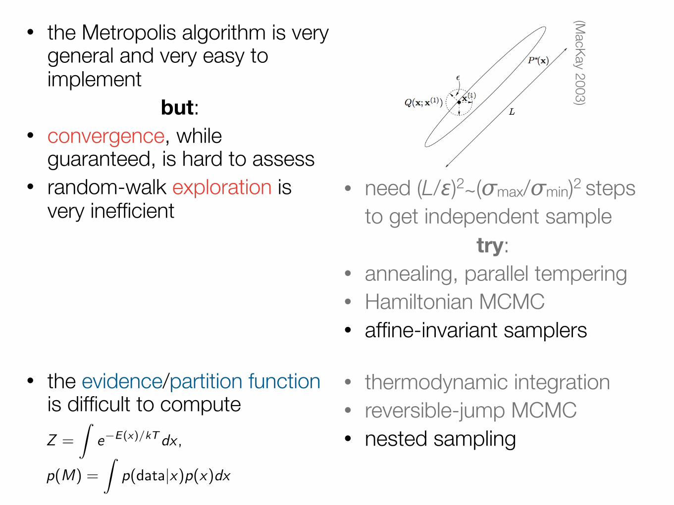
• the Metropolis algorithm is very general and very easy to implement


but:• convergence, while

guaranteed, is hard to assess• random-walk exploration is

very inefficient




very inefficient• need (L/ε)2∼(σmax/σmin)2 steps

to get independent sample

(MacK

ay 2003)




very inefficient• need (L/ε)2∼(σmax/σmin)2 steps

to get independent sampletry:

• annealing, parallel tempering• Hamiltonian MCMC• affine-invariant samplers

(MacK

ay 2003)




very inefficient

• the evidence/partition function is difficult to compute

• need (L/ε)2∼(σmax/σmin)2 steps to get independent sample

try:• annealing, parallel tempering• Hamiltonian MCMC• affine-invariant samplers

(MacK

ay 2003)

Z =

�e−E(x)/kTdx ,

p(M) =

�p(data|x)p(x)dx




very inefficient

• the evidence/partition function is difficult to compute

• need (L/ε)2∼(σmax/σmin)2 steps to get independent sample

try:• annealing, parallel tempering• Hamiltonian MCMC• affine-invariant samplers

• thermodynamic integration• reversible-jump MCMC• nested sampling

(MacK

ay 2003)

Z =

�e−E(x)/kTdx ,

p(M) =

�p(data|x)p(x)dx

Nested sampling(Skilling 2006)


Z =

�L(θ)π(θ)dθ =

�L(X )dX

X (λ) =

�

L(θ)>λπ(θ)dθ


Z =

�L(θ)π(θ)dθ =

�L(X )dX

X (λ) =

�

L(θ)>λπ(θ)dθ

Z =�

i

wiLi


Z =

�L(θ)π(θ)dθ =

�L(X )dX

X (λ) =

�

L(θ)>λπ(θ)dθ

Z =�

i

wiLi

• Z is dominated by a range–H ± √d in log X, so we explore X linearly in log X


Z =

�L(θ)π(θ)dθ =

�L(X )dX

X (λ) =

�

L(θ)>λπ(θ)dθ

Z =�

i

wiLi


• choose each Xi randomly, subject to Xi < Xi–1


Z =

�L(θ)π(θ)dθ =

�L(X )dX

X (λ) =

�

L(θ)>λπ(θ)dθ

Z =�

i

wiLi



• in practice, choose θ fromπ(θ), subject to L(θi) > L(θi–1)


Z =

�L(θ)π(θ)dθ =

�L(X )dX

X (λ) =

�

L(θ)>λπ(θ)dθ

Z =�

i

wiLi



• in practice, choose θ fromπ(θ), subject to L(θi) > L(θi–1) X0 = 1, Xi = tiXi−1, ti ∈ [0, 1]





• working with a cloud of Nlive points, keep replacing the least-L member, use it as Xi

X0 = 1, Xi = tiXi−1, p(ti ) = NtN−1i ∈ [0, 1]






•

X0 = 1, Xi = tiXi−1, p(ti ) = NtN−1i ∈ [0, 1]

logXi � (−i ±√i)/N

Z =�

i

wiLi , wi =Xi−1 − Xi+1

2






•

• stop when Z convergesX0 = 1, Xi = tiXi−1, p(ti ) = NtN−1

i ∈ [0, 1]


Z =�

i


2






•

• stop when Z convergesX0 = 1, Xi = tiXi−1, p(ti ) = NtN−1

i ∈ [0, 1]


Z =�

i


2

see bit.ly/multinestby Farhan Feroz, Hobson, Bridges

Affine–invariant sampling(Goodman–Weare 2010)


π(x) ∝ exp

�−(x1 − x2)2

2�− (x1 + x2)2

2

�

hard to sample!


π(x) ∝ exp

�−(x1 − x2)2

2�− (x1 + x2)2

2

�

hard to sample!

πA(y) ∝ exp

�− (y1 + y2)2

2

�y1 =

x1 − x2√�

, y2 = x1 + x2

much better!

• a sampler with affine-invariant transition probabilities would conform automatically to any coordinates (cf. simplex optimization)


π(x) ∝ exp

�−(x1 − x2)2

2�− (x1 + x2)2

2

�

hard to sample!

πA(y) ∝ exp

�− (y1 + y2)2

2

�y1 =

x1 − x2√�

, y2 = x1 + x2

much better!


• G–W ensemble sampler: to update each walker xi (i=1,..,N) in turn propose xi → xj + z⋅(xk – xj), k ≠ j with density g(z) ∝ 1/√z for z ∈ [1/a,a] accept with Metropolis


π(x) ∝ exp

�−(x1 − x2)2

2�− (x1 + x2)2

2

�

hard to sample!

πA(y) ∝ exp

�− (y1 + y2)2

2

�y1 =

x1 − x2√�

, y2 = x1 + x2

much better!

xi

xj

xi,proposed



• the final ensemble approximates the posterior


π(x) ∝ exp

�−(x1 − x2)2

2�− (x1 + x2)2

2

�

hard to sample!

πA(y) ∝ exp

�− (y1 + y2)2

2

�y1 =

x1 − x2√�

, y2 = x1 + x2

much better!

xi

xj

xi,proposed



• the final ensemble approximates the posterior


π(x) ∝ exp

�−(x1 − x2)2

2�− (x1 + x2)2

2

�

hard to sample!

πA(y) ∝ exp

�− (y1 + y2)2

2

�y1 =

x1 − x2√�

, y2 = x1 + x2

much better!

see dan.iel.fm/emceeby Daniel Foreman-Mackey et al.

xi

xj

xi,proposed

Discussion

Discussion

God is always in the details...

Discussion

God is always in the details......but the transcendent is experienced, never proved

Discussion


Trust no one...

Discussion


Trust no one......because there’s no free lunch

Discussion


Trust no one......because there’s no free lunch(not even with genetically engineered algorithms)

Discussion



Parallelization is hard...

Discussion



Parallelization is hard......but Gaussian integrals are easy

Discussion



Parallelization is hard......but Gaussian integrals are easy

But harnessing the power of stochastic physical systems,that’s just cool!

Backup slides

Michele Vallisneri, Jet Propulsion Laboratory

Copyright 2013 California Institute of Technology

GW science in a nutshell:GW detection with addition, subtraction, and multiplication

�4 �2 0 2 4�3

�2

�1

0

1

2

3

�4 �2 0 2 4�3

�2

�1

0

1

2

3

�4 �2 0 2 4�3

�2

�1

0

1

2

3

+ =

(SNR = 5)

data = signal + noise

therefore: noise = data – signal; to assess detection,we ask which instance of noise is more probable?

or�4 �2 0 2 4�3

�2

�1

0

1

2

3

�4 �2 0 2 4�3

�2

�1

0

1

2

3

�4 �2 0 2 4�3

�2

�1

0

1

2

3

(no signal)


or�4 �2 0 2 4�3

�2

�1

0

1

2

3

�4 �2 0 2 4�3

�2

�1

0

1

2

3

�4 �2 0 2 4�3

�2

�1

0

1

2

3

(no signal)

�4 �2 0 2 4�3

�2

�1

0

1

2

3

�4 �2 0 2 4�3

�2

�1

0

1

2

3

�4 �2 0 2 4�3

�2

�1

0

1

2

3

= –

�4 �2 0 2 4�3

�2

�1

0

1

2

3

�4 �2 0 2 4�3

�2

�1

0

1

2

3

�4 �2 0 2 4�3

�2

�1

0

1

2

3

�4 �2 0 2 4�3

�2

�1

0

1

2

3

�4 �2 0 2 4�3

�2

�1

0

1

2

3

�4 �2 0 2 4�3

�2

�1

0

1

2

3

(signal hidden in noise,so we subtract it out)


or�4 �2 0 2 4�3

�2

�1

0

1

2

3

�4 �2 0 2 4�3

�2

�1

0

1

2

3

�4 �2 0 2 4�3

�2

�1

0

1

2

3

(no signal)

�4 �2 0 2 4�3

�2

�1

0

1

2

3

�4 �2 0 2 4�3

�2

�1

0

1

2

3

�4 �2 0 2 4�3

�2

�1

0

1

2

3

= –

�4 �2 0 2 4�3

�2

�1

0

1

2

3

�4 �2 0 2 4�3

�2

�1

0

1

2

3

�4 �2 0 2 4�3

�2

�1

0

1

2

3

�4 �2 0 2 4�3

�2

�1

0

1

2

3

�4 �2 0 2 4�3

�2

�1

0

1

2

3

�4 �2 0 2 4�3

�2

�1

0

1

2

3

(signal hidden in noise,so we subtract it out)

the ratio of probabilities is ~ exp SNR2/2, (here ~ 270,000)

an intuitive interpretation of this processis in terms of correlation products/matched filtering

0 20 40 60 80 100

�1.0

�0.5

0.0

0.5

1.0

0 20 40 60 80 1000.0

0.5

1.0

1.5

0 20 40 60 80 100

�2

�1

0

1

2

0 20 40 60 80 100

�1.0

�0.5

0.0

0.5

1.0

1.5

2.0

0 20 40 60 80 100

�1.0

�0.5

0.0

0.5

1.0

0 20 40 60 80 100

�1.0

�0.5

0.0

0.5

1.0

x = →∫

25

x = →∫

3.39


detectordata

signal“template”

(Chad Hanna)


�10 0 10 20 30 400.00

0.02

0.04

0.06

0.08

no signal with signal

threshold

detectordata

signal“template”

(Chad Hanna)

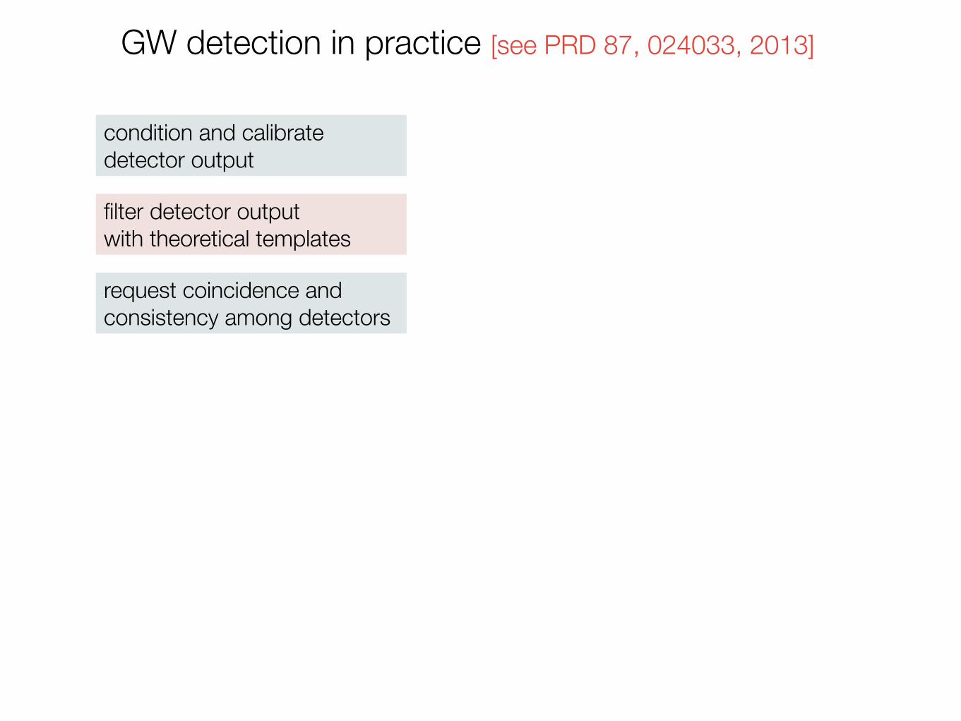
30 GW detection in practice [see PRD 87, 024033, 2013]

filter detector outputwith theoretical templates



condition and calibrate detector output




request coincidence and consistency among detectors





apply data-quality cutsand signal vetos






estimate statistical significance

(estimate background, using coincidence between time slides)








follow up candidateswith detection checklist








claim detection!


get upper limit

(estimate efficiency from injections, number of galaxies within horizon)








claim detection!


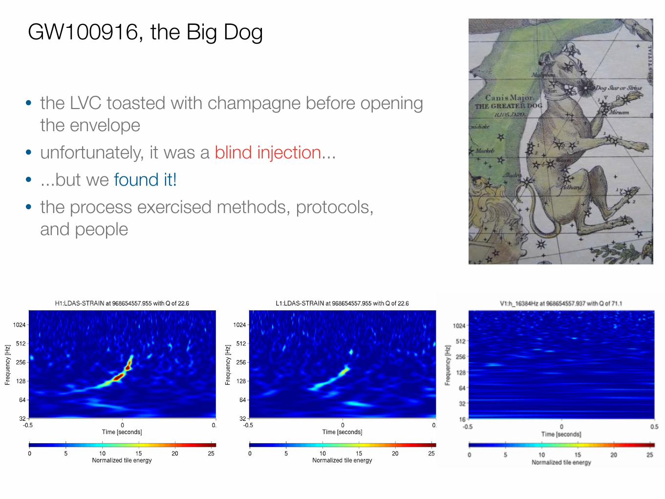
GW100916, the Big Dog


• the LVC toasted with champagne before opening the envelope



• unfortunately, it was a blind injection...



• unfortunately, it was a blind injection...• ...but we found it!



• unfortunately, it was a blind injection...• ...but we found it!• the process exercised methods, protocols,

and people



• unfortunately, it was a blind injection...• ...but we found it!• the process exercised methods, protocols,

and people• it showed the perils of theory, experiment, software

O =P(AG|s)

P(GR|s)=P(AG)

�p(s |θi ,a) p(θi ,a) dθi ,a

P(GR)�p(s |θi) p(θi) dθi

evidence (= marginal likelihood)for AG and GR models

model priors

likelihood

parameter priors

AG parameters

GR parameters

x is a normal random variable with zero meanand unit variance (a function on noise realization)

renormalized odds ratios (model priorsand Occam factors cancel out, see paper)

O�AG = e

x2/2+x√2(1−FF) SNR+(1−FF) SNR2

O�GR = e

x2/2

background: true signal is GR detection efficiency: true signal is AG

we design a decision scheme (“AG or GR?”) with the Bayesian odds ratio as the detection statistic; we set a threshold and claim detection when

O O∗

O > O∗

SNR=10FF=0.95

SNR=15FF=0.95

5% false alarms

logO�AGlogO�

GR

distributionof

distributionof

88%detections

99%detections

0.10

0.05

00 5 10 15 205 10 15 20

thresholdlogO∗ = 2

for strong signals, and are remarkably simple functions of FF and SNR alone. For a fixed false-alarm rate, we then askwhat SNR yields 50%-efficient AG detection, as a function of FF

!" !# !$ !% !& !' !( !) *

+,-./0,-,1203040)*!&)**5***

)5***

)*

)*5***

)5***

)*

)**

-67)*

3040)*!"

SNR required forAG detectionwith 50% efficiency

number of events in a volume-limited search to yield that SNR as the loudest event

only very strong AG effects (FF of 0.9–0.99) would be seen in volume-limited searches, so GR tests may have to wait for third-generation ground-based detectors, or for space detectors

O�GR O

�AG

if model signals (GR) differ from true signals (MG) with the same parameters, the best-fitting template will be displaced by theoretical error, which isSNR-independent [see Cutler & Vallisneri 2007]

an application [Vallisneri and Yunes, arXiv/1301.2627]:“fundamental” bias versus the detection of modified gravity

manifold of truesignals

approximated signals

hGR(θtrue)

hAPP(θtrue)

hGR(θbest)∆θ

δh

4

where (a, b) ∈ Z, with (a, b) > (−10,−15) [44].

In this paper we concentrate on phasing cor-

rections by setting α = 0 and choosing b ∈{−7,−6,−5,−4,−3,−2,−1, 1, 2}. Different values of brepresent different types of MG effects: b = −7 cor-

responds to the leading–PN-order correction in Brans–

Dicke theory [8, 9, 14–16, 23, 45] or in Einstein–dilaton–

Gauss–Bonnet gravity [19, 46]; b = −3 to the leading-

order term in a phenomenological massive graviton the-

ory [9, 11, 12, 14, 22, 25, 45], b ≥ −5 (but �= −4) to

the modified-PN scheme of Refs. [4–7], and b = −1 to

dynamical Chern–Simons gravity [19, 21, 47]. Notice, in

particular, that the modified-PN scheme is clearly a sub-

case of the ppE scheme. We omit b = 0 because the

resulting correction would be degenerate with an arbi-

trary constant in the phase. We do not consider b < −7

because the values that we study provide enough infor-

mation to observe a consistent trend as b becomes more

negative. Moreover, for b ≤ −7, binary pulsar observa-

tions can do a better job at constraining modified gravity

theories than GWs observations [48]. We do not consider

b > 2, as this would correspond to terms of higher than

3.5 PN order, which we do not account for in the ΨGR.

B. Quantifying the bias

Let us assume that a GW detection is reported for a

dataset s that contains the waveform

hfull(�θtr) = h(�θtr) + δh(�θtr), (8)

where �θtr is the vector of parameters that describes the

GW source and source–detector geometry, h is the ap-

proximated waveform family used to filter the data, and

δh is the unmodeled correction to h. Following Cutler

and Vallisneri [30], we compute the theoretical error δ�θthinduced by matched-filtering with h instead of hfull.

The theoretical error δ�θth is defined as the displace-

ment �θbf − �θtr between the true parameters �θtr and the

best-fit parameters �θbf that would maximize the like-

lihood in the absence of noise. When δh(�θtr) is neg-

ligibly small, �θbf = �θtr; as δh(�θtr) grows in magni-

tude, �θbf is displaced further and further away along the

parameter-space direction in which h(�θbf) can reproduce

h(�θtr) + δh(�θtr) most closely.

To leading order in δh, δ�θth is given by [30]

δ�θth = (F−1bf )

αβ�h,β(

�θbf)��δh(�θbf)

�, (9)

where h,β = ∂h/∂θβ are partial derivatives of the wave-

form with respect to source parameters, Fαβ = (h,α|h,β)

is the Fisher matrix, here evaluated at θbf , and

(g1|g2) = 4Re

� ∞

0

g1∗(f)g2(f)

Sn(f)df, (10)

is the noise-weighted signal inner product, with Sn(f)the one-sided power spectral density of detector noise

(see, e.g., [38]). The inner product defines a signal norm|h| by way of |h|2 = (h|h).In Eq. (9), the waveform correction δh is projected

onto the waveform derivatives, and the projection cosines

are mapped into parameter errors by the inverse Fisher

matrix F−1, thus taking into account possible parameter

covariances. Note that the resulting δ�θth is independent

of the detection SNR, since both F and (h,β(θbf)|δh(θbf))are quadratic in the waveform amplitude.

Equation (9) is only accurate for small δ�θth—more pre-

cisely, for perturbations small enough that h(�θbf−δ�θth) �h(�θbf)− h,αδθαth. Cutler and Vallisneri [30] discuss more

sophisticated versions of Eq. (9) that can be applied to

larger perturbations, but in this paper we adopt the sim-

pler Eq. (9), not least because the other ingredients in

our formulation depend on δh(�θtr) being small.

C. Detecting modified gravity

Following Vallisneri [31] (see also [3]), we define a MG

correction δh to the signal h to be detectable when the

odds ratio of the Bayesian evidences for the MG and

pure-GR scenarios, used as a detection statistic, is large

enough that the false-alarm probability of favoring the

MG hypothesis when GR is in fact correct is suitably

small. More precisely, we compute the odds ratio

O =P (MG|s)

P (GR|s)=

P (MG)�p(s|�θ,�λ) p(�θ,�λ) dkθ dmλ

P (GR)�p(s|�θ) p(�θ) dkθ

,

(11)

where P (MG) and P (GR) are the prior probabilities that

MG and GR are correct, p(s|�θ,�λ) is the likelihood that

the detector data s contains the MG waveform h(�θ) +δh(�θ,�λ), p(s|�θ) is the likelihood that s contains the pure-

GR waveform h(�θ), and p(�θ,�λ) = p(�θ)p(�λ) and p(�θ) are

the prior probability densities for the source parameters

�θ and the MG parameters �λ.If the true signal is MG, using MG templates would

improve the fit to the data and increase the maximum

value attained by the MG likelihood relative to the GR

likelihood. On the other hand, the evidence for the more

complicated, higher-dimensional MG model is reduced

by the smaller prior mass within the support of the

likelihood—the mechanism by which Bayesian inference

embodies Occam’s principle of parsimony. As signals get

stronger, the improvement in the likelihood grows expo-

nentially with the (squared) detection SNR, and eventu-

ally it overcomes the effect of the priors.

Even if we fix the true signal, the odds ratio O remains

a random variable, because it depends on the realization

of detector noise, by way of the likelihoods. For suffi-

ciently large detection SNR, it can be shown [31] that

Eq. (11) becomes remarkably simple: for the cases when

the underlying signal is pure-GR or MG respectively, we

representing modified gravity as “parametrized post-Einstein,”we compare the MG SNRdetect with the SNRbias where δθth > δθstat

3

Mismodeling bias is remedied by deriving ever more

accurate solutions to the field equations: for binary in-

spirals, this goal is currently pursued by pushing the

PN approximation to higher orders, and by integrating

together PN and numerical-relativity results with ana-

lytical resummation and fitting techniques, such as the

effective-one-body scheme. Instrumental bias is reduced

by careful detector modeling and characterization. As-

trophysical bias is expected to be irrelevant for most

ground-based binary observations; but even if this were

not the case, astrophysical effects should present them-

selves differently (or not at all) in observations of differ-ent systems, whereas fundamental bias, if present, would

appear equally in all observed systems.

In this paper, we concentrate on the inspiral signals

from compact-binary coalescences. We consider inspirals

that are circular and adiabatic, with negligible spin ef-

fects, and neglect mismodeling bias by assuming the GW

emission is well-described by the restricted PN waveform

in the frequency-domain, stationary-phase approxima-

tion [38–41]. In GR, the resulting signals can be written

as

hGR(f) = AGR(f)eiΨGR(f) , (1)

where AGR(f) = Au−7/6 [1 + · · · ] (we neglect PN ampli-

tude corrections, symbolized with ellipses in the above

equation), u = πMf is the reduced frequency, M =

η3/5M the chirp mass, η = m1m2/M2 the symmetric

mass ratio, M = m1+m2 the total mass, and f the GW

frequency. The constant amplitude A depends on the

chirp mass, the luminosity distance, and the detector’s

antenna patterns [38–41]. The quantity ΨGR(f) in Eq.

(1) is the GW phase, given in the PN approximation by

ΨGR = 2πftc − φc −π

4

+3u−5/3

128

�1 +

7�

k=2

�ψk +

1

3ψk log(u)

�η−k/5uk/3

�,

(2)

where the constant coefficients (ψk, ψk) can be found (for

instance) in Ref. [30].

Under these assumptions, the unmodeled corrections

enumerated above can be represented by a continuous

and (in principle) predictable deformation of the GW

phase Ψ(f) and amplitude A(f). The particular defor-

mation depends on the systematic effect. For mismod-

eling, we expect corrections within the structure of the

PN series (δA ∝ f−7/6+kA/3 for the amplitude and δΨ ∝f−5/3+kφ/3 for the phase, with integers kA, kφ > 0), be-

yond the highest known perturbative order (i.e., kA > 5

for the amplitude and kφ > 7 for the phase).

For astrophysical effects, we expect corrections to arise

almost always with “negative” PN exponents [33, 36, 37,

42]. For example, an accretion disk [42], the presence of a

third body [36], and orbital eccentricity [42] all introduce

GW phase corrections δΨ ∝ f−5/3−k�φ , with integer k�φ >

0. Physically, this frequency-dependence corresponds to

astrophysical effects becoming less important for tighter

binaries, where strong-field effects become dominant.

Moving on to unmodeled corrections originating from

fundamental physics, the amplitude and phase deforma-

tions δA and δΨ can always be expressed as sums of fre-

quency powers, provided that δA and δΨ remain analyticat all frequencies sampled during the inspiral:

δA = AGR(f)K�

k=1

αkuak , δΨ(f) =

K�

k=1

βkubk , (3)

where (αk,βk, ak, bk) ∈ R for all k, and where we have

included the AGR prefactor in δA. We have neglected

possible logarithmic terms for simplicity, but they can

be included easily in the same fashion. This ppE model

introduces 4K new parameters in the waveform; the sim-

plest version of this model would allow only a single ex-

ponent:

δA = AGR(f)αua , δΨ(f) = β ub . (4)

Indeed, it can be shown that such a parametric defor-

mation is sufficiently general to model all known MG

corrections to the waveform to leading PN order [2, 3],

provided that the two tensor polarizations are dominant,

as in GR. Otherwise, a second term would be needed in

the phase and amplitude [43, 44].

Furthermore, a convincing argument can be made that

a and b should be restricted to a few discrete values [44].

Suppose that the adiabatic-inspiral waveform is derived

from an energy-balance equation with modified binding

energy and flux of the form

E = E0 v2�1 + (· · · )PN + δE vk

�, (5)

E = E0 v10

�1 + (· · · )PN + δE vm

�, (6)

where v is the relative velocity of the binary components,

ellipses stand for higher-order PN terms, and E0, E0, δEand δE are all constants that may depend on the source

parameters and on the MG coupling constants. The ex-

ponents k and m must be integers, otherwise E or Ewould not be analytic, and we would lose the guaran-

tee that the equations have a unique solution of hyper-

bolic character by the Picard–Lindelof theorem3. Fur-

thermore, we must have k ≥ −2 and m ≥ −10, otherwise

E and E would not reduce to the GR result in the weak-

field limit. These constraints lead to the deformations

δA = AGR(f)αua/3 , δΨ(f) = β ub/3 , (7)

3 Given the differential equation dy/dt = f(t, y(t)), with initialvalue y(t0) = y0, a unique solution exists for all t ∈ (t0−�, t0+�)provided that f is Lipschitz continuous in y and continuous in t.A noninteger value of k and m would lead to a differential equa-tion with a non-Lipschitz continuous source term, with possibleloss of uniqueness.

3





















as












4

+3u−5/3

128

�1 +

7�

k=2

�ψk +

1

3ψk log(u)

�η−k/5uk/3

�,

(2)
























δA = AGR(f)K�

k=1

αkuak , δΨ(f) =

K�

k=1

βkubk , (3)







ponent:













E = E0 v2�1 + (· · · )PN + δE vk

�, (5)

E = E0 v10

�1 + (· · · )PN + δE vm

�, (6)













3





















as












4

+3u−5/3

128

�1 +

7�

k=2

�ψk +

1

3ψk log(u)

�η−k/5uk/3

�,

(2)
























δA = AGR(f)K�

k=1

αkuak , δΨ(f) =

K�

k=1

βkubk , (3)







ponent:













E = E0 v2�1 + (· · · )PN + δE vk

�, (5)

E = E0 v10

�1 + (· · · )PN + δE vm

�, (6)












3





















as












4

+3u−5/3

128

�1 +

7�

k=2

�ψk +

1

3ψk log(u)

�η−k/5uk/3

�,

(2)
























δA = AGR(f)K�

k=1

αkuak , δΨ(f) =

K�

k=1

βkubk , (3)







ponent:













E = E0 v2�1 + (· · · )PN + δE vk

�, (5)

E = E0 v10

�1 + (· · · )PN + δE vm

�, (6)












6

in approximating h(�θtr + δ�θstat) − h(�θtr) as h,αδθαstat besufficiently small (0.1 in norm) on most (95%) of the 1–σerror surface described by (F−1)αβ . For the theoreticalerrors, we require that the FFs computed in the two waysdescribed below Eq. (13) be consistent to 1%.

III. ANALYSIS AND RESULTS

We examine three representative binary GW sourcesfor second-generation interferometric detectors such asAdvanced LIGO [50]: neutron-star–neutron-star bina-ries with (1.4+1.4)M⊙ component masses; neutron-star–black-hole binaries with (1.4 + 5)M⊙ masses; and black-hole–black-hole binaries with (5 + 10)M⊙ masses.

We concentrate on the inspiral phase of coalescence,which we model as quadrupolar and adiabatically quasi-circular with 3.5PN-accurate phasing. We truncate thewaves at the innermost stable circular orbit of a point-particle in a Schwarzschild background (assuming GR),and we neglect spin effects and PN amplitude corrections.The resulting waveforms are described by nine parame-ters: the two masses (or the chirp and reduced masses),the time and inspiral phase at coalescence, two sky-position angles, two angles that describe the binary incli-nation and GW polarization, and the luminosity distance(see [30] and [3] for a similar waveform prescription).We assume a simultaneous detection by three second-generation detectors with the LIGO Hanford, LIGO Liv-ingston, and Virgo geometries and relative delays [51],and with identical broadband-configuration power spec-tral densities, as given by Eq. (10) of [3]. Furthermore,we assume that GW-detector noise is Gaussian and sta-tionary, as required by the Cutler–Vallisneri [30] and Val-lisneri [31] formalisms.

For these systems, we consider ppE phasing correctionsδΨ as described in Sec. II A, and we compare SNRbias

and SNRdetect as a function of the MG-correction mag-nitude β for a range of exponents b. For each mass com-bination, each b, and each β, we randomly select 1,000configurations of the phase and angle parameters fromthe appropriate uniform distributions (e.g., sky positionsare chosen randomly on the celestial sphere). The lumi-nosity distance is reabsorbed in the SNR scaling, whilethe time of coalescence has no effect on our computa-tion. For each configuration we compute SNRdetect andSNRbias, and we report their median values. The con-dition maxα δθαth/δθ

αstat = 1 that yields the latter is al-

most invariably satisfied first for the chirp-mass parame-ter. Statistical fluctuations around the median turn outto be rather small (a few percent).

The δ�θstat consistency check is satisfied for detectionSNRs ranging from 10 to 100, typically ∼ 50, but ourresults for lower SNRs should be at least representativeof trends. The δ�θth check is satisfied for a maximum βthat depends on b, and which sets the largest β that weinvestigate. By contrast, the smallest β that we studycorresponds to min(SNRdetect, SNRbias) = 100, a rela-

!"#!"

!"#$%

$%#$%

"!&'()(*)"!&+,-.

FIG. 1. SNRdetect

(solid curves) and SNRbias

(dashed

curves) as a function of β for b = −7,−6,−5,−4,−3,−2,−1, 1and 2 (left to right), for a NS–NS system with (m1,m2) =

(1.4, 1.4)M⊙ (top), a NS–BH system with (m1,m2) =

(1.4, 5)M⊙ (mid) and a BH–BH system (bottom) with

(m1,m2) = (5, 10)M⊙. The symbols in the top plot are de-

scribed in the main text.

tively large detection SNR that would be achieved veryrarely in volume-limited searches [52].Figure 1 presents the main results of this paper, with

the solid curves plotting SNRdetect (once again, the detec-tion SNR above which MG can be detected positively),and the dashed curves plotting SNRbias (the SNR abovewhich the largest ratio of fundamental error to statisticalerror reaches one). Both sets of curves are plotted as afunction of the MG-correction magnitude β; the curves ineach set correspond to b = −7,−5,−4,−3,−2,−1, 1, and2, from left to right as labeled. The top, mid, and bottompanels report results for our (1.4+1.4)M⊙, (1.4+5)M⊙,and (5 + 10)M⊙ systems, respectively.

This figure reveals a few interesting features. First,for the same detection SNR, more massive systems re-quire larger β before MG can be detected. This musthappen because the larger the mass, the fewer the num-ber of useful GW cycles in the detector’s band, so thesignals become relatively featureless, and higher FFs can


3





















as












4

+3u−5/3

128

�1 +

7�

k=2

�ψk +

1

3ψk log(u)

�η−k/5uk/3

�,

(2)
























δA = AGR(f)K�

k=1

αkuak , δΨ(f) =

K�

k=1

βkubk , (3)







ponent:













E = E0 v2�1 + (· · · )PN + δE vk

�, (5)

E = E0 v10

�1 + (· · · )PN + δE vm

�, (6)












3





















as












4

+3u−5/3

128

�1 +

7�

k=2

�ψk +

1

3ψk log(u)

�η−k/5uk/3

�,

(2)
























δA = AGR(f)K�

k=1

αkuak , δΨ(f) =

K�

k=1

βkubk , (3)







ponent:













E = E0 v2�1 + (· · · )PN + δE vk

�, (5)

E = E0 v10

�1 + (· · · )PN + δE vm

�, (6)












6

in approximating h(�θtr + δ�θstat) − h(�θtr) as h,αδθαstat besufficiently small (0.1 in norm) on most (95%) of the 1–σerror surface described by (F−1)αβ . For the theoreticalerrors, we require that the FFs computed in the two waysdescribed below Eq. (13) be consistent to 1%.

III. ANALYSIS AND RESULTS

We examine three representative binary GW sourcesfor second-generation interferometric detectors such asAdvanced LIGO [50]: neutron-star–neutron-star bina-ries with (1.4+1.4)M⊙ component masses; neutron-star–black-hole binaries with (1.4 + 5)M⊙ masses; and black-hole–black-hole binaries with (5 + 10)M⊙ masses.

We concentrate on the inspiral phase of coalescence,which we model as quadrupolar and adiabatically quasi-circular with 3.5PN-accurate phasing. We truncate thewaves at the innermost stable circular orbit of a point-particle in a Schwarzschild background (assuming GR),and we neglect spin effects and PN amplitude corrections.The resulting waveforms are described by nine parame-ters: the two masses (or the chirp and reduced masses),the time and inspiral phase at coalescence, two sky-position angles, two angles that describe the binary incli-nation and GW polarization, and the luminosity distance(see [30] and [3] for a similar waveform prescription).We assume a simultaneous detection by three second-generation detectors with the LIGO Hanford, LIGO Liv-ingston, and Virgo geometries and relative delays [51],and with identical broadband-configuration power spec-tral densities, as given by Eq. (10) of [3]. Furthermore,we assume that GW-detector noise is Gaussian and sta-tionary, as required by the Cutler–Vallisneri [30] and Val-lisneri [31] formalisms.

For these systems, we consider ppE phasing correctionsδΨ as described in Sec. II A, and we compare SNRbias

and SNRdetect as a function of the MG-correction mag-nitude β for a range of exponents b. For each mass com-bination, each b, and each β, we randomly select 1,000configurations of the phase and angle parameters fromthe appropriate uniform distributions (e.g., sky positionsare chosen randomly on the celestial sphere). The lumi-nosity distance is reabsorbed in the SNR scaling, whilethe time of coalescence has no effect on our computa-tion. For each configuration we compute SNRdetect andSNRbias, and we report their median values. The con-dition maxα δθαth/δθ

αstat = 1 that yields the latter is al-

most invariably satisfied first for the chirp-mass parame-ter. Statistical fluctuations around the median turn outto be rather small (a few percent).

The δ�θstat consistency check is satisfied for detectionSNRs ranging from 10 to 100, typically ∼ 50, but ourresults for lower SNRs should be at least representativeof trends. The δ�θth check is satisfied for a maximum βthat depends on b, and which sets the largest β that weinvestigate. By contrast, the smallest β that we studycorresponds to min(SNRdetect, SNRbias) = 100, a rela-

!"#!"

!"#$%

$%#$%

"!&'()(*)"!&+,-.

FIG. 1. SNRdetect

(solid curves) and SNRbias

(dashed

curves) as a function of β for b = −7,−6,−5,−4,−3,−2,−1, 1and 2 (left to right), for a NS–NS system with (m1,m2) =

(1.4, 1.4)M⊙ (top), a NS–BH system with (m1,m2) =

(1.4, 5)M⊙ (mid) and a BH–BH system (bottom) with

(m1,m2) = (5, 10)M⊙. The symbols in the top plot are de-

scribed in the main text.

tively large detection SNR that would be achieved veryrarely in volume-limited searches [52].Figure 1 presents the main results of this paper, with

the solid curves plotting SNRdetect (once again, the detec-tion SNR above which MG can be detected positively),and the dashed curves plotting SNRbias (the SNR abovewhich the largest ratio of fundamental error to statisticalerror reaches one). Both sets of curves are plotted as afunction of the MG-correction magnitude β; the curves ineach set correspond to b = −7,−5,−4,−3,−2,−1, 1, and2, from left to right as labeled. The top, mid, and bottompanels report results for our (1.4+1.4)M⊙, (1.4+5)M⊙,and (5 + 10)M⊙ systems, respectively.

This figure reveals a few interesting features. First,for the same detection SNR, more massive systems re-quire larger β before MG can be detected. This musthappen because the larger the mass, the fewer the num-ber of useful GW cycles in the detector’s band, so thesignals become relatively featureless, and higher FFs can

at least for simple circular inspirals, stealth bias (significant δθth, non-detectable MG) is generic![but see arXiv/1301.2627]

the Mock LISA Data Challenges: successfully fosteringand consolidating collaborative data-analysis development

• five challenges completed between 2006 and 2011

• 70 participants, 25 institutions 30+ publications

• demonstrated the detection and parameter estimation of all major LF GW source classes, using a great variety of methods

• lisatools.googlecode.comlisasolve.googlecode.com

• acknowledged model for LISA Pathfinder and the International Pulsar-Timing Array

Markov Chain Monte Carlo: the ultimate multitool - TAPIR Group at

Documents

Transcript of Markov Chain Monte Carlo: the ultimate multitool - TAPIR Group at