Market Structure and Productivity: A Concrete Example

Chad Syverson* University of Chicago

July 2001

* Contact Information: Department of Economics, University of Chicago; 1126 E. 59th St.; Chicago, IL 60637; e-mail: syverson@midway.uchicago.edu I thank seminar participants at the NBER Summer Institute, the Brookings Institution, and the Center for Economic Studies for their comments. Mark Roberts made several helpful suggestions regarding an earlier draft. I am also grateful to John Haltiwanger, Rachel Kranton, Mike Pries, Plutarchos Sakellaris, and John Shea for their instruction and guidance. Funding from a Brookings Research Fellowship is appreciatively acknowledged. The research in this paper was conducted while the author was a research associate at the Center for Economic Studies, U.S. Bureau of the Census. Research results and conclusions expressed are those of the author and do not necessarily indicate concurrence by the Bureau of the Census or the Center for Economic Studies.

Market Structure and Productivity: A Concrete Example

Abstract

This paper shows that imperfect output substitutability explains part of the observed persistent plant-level productivity dispersion. Specifically, as substitutability in a market increases, the market’s productivity distribution exhibits falling dispersion and higher central tendency. The proposed mechanism behind this result is truncation of the distribution from below as increased substitutability shifts demand to lower-cost plants and drives inefficient plants out of business. In a case study of the ready-mixed concrete industry, I examine the impact of one manifestation of this effect, driven by geographic market segmentation resulting from transport costs. A theoretical foundation is presented characterizing how differences in the density of local demand impact the number of producers and the ability of customers to choose between suppliers, and through this, the equilibrium productivity and output levels across regions. I also introduce a new method of obtaining plant-level productivity estimates that is well suited to this application and avoids potential shortfalls of commonly used procedures. I use these estimates to empirically test the presented theory, and the results support the predictions of the model. Local demand density has a significant influence on the shape of plant-level productivity distributions, and accounts for part of the observed intra-industry variation in productivity, both between and within given market areas.

Recent empirical explorations have left little doubt about the magnitude of plant-level

total factor productivity variation: it is enormous. This heterogeneity is also persistent. Perhaps

surprisingly, much of the variation cannot be explained by differences between (even narrowly

defined) industries. For example, studies reviewed in Bartelsman and Doms (2000) have found

85th-to-15th TFP percentile ratios of between 2:1 and 4:1 within various four-digit SIC industries.

Productivity growth also exhibits huge within-industry dispersion: Haltiwanger (1997) finds that

only 8.5% of productivity growth variation is explained by four-digit industry. An assortment of

theoretical work has arisen attempting to explain the sources of such diversity. The great

majority of this research focuses on supply-side (production) causes, such as idiosyncratic

technology shocks, management influences, R & D efforts, or investment patterns.1

In this paper I turn my attention to the demand (i.e., output market) side, and look at how

market structure can cause such within-industry heterogeneity to persist.2 I argue that across-

plant differences in output market conditions are partially responsible for observed persistent

productivity dispersion—and in fact, the dispersion of that dispersion. The specific channel

through which this posited influence flows is variable output substitutability in a world of

product differentiation. The more difficult it is for consumers to switch between competing

suppliers, the greater the amount of dispersion that can be sustained. I will focus here on a

particular component of substitutability, geographic market segmentation created by transport

costs, and examine its impact on productivity dispersion within a single industry. The purpose

of this paper, however, is not to give the final word on transport costs and productivity in a

particular industry. Instead, I hope to show through a detailed case study—where many

potentially confounding factors are held constant—how transport costs as well as other

substitutability factors might impact productivity variation and levels throughout the economy.

The rationale for using output market effects, and substitutability specifically, to explain

the degree of within-industry productivity heterogeneity is more readily apparent when one

considers how such wide efficiency variation can exist in equilibrium. After all, output should

tend to be reallocated to more productive plants over time. High-productivity plants are able to

produce output at lower cost than industry rivals, allowing them to grab additional market share

1 Just a sampling includes Jovanovic (1982) and Ericson and Pakes (1995). See Bartelsman and Doms

(2000) for a review of this literature.

1

2 There are supply-side stories that can explain persistent dispersion as well. I simply want to highlight another piece of the puzzle, to my knowledge not previously formalized, from the demand side.

by undercutting their opponents’ prices without sacrificing profit rates. One might expect this

process to redistribute most or all of an industry’s production to a select few high-productivity

plants. Output and productivity patterns like this are not usually observed in the data, however;

the overwhelming weight of empirical evidence indicates widely varying producer productivity

levels within nearly every industry.

What prevents this output reallocation process from occurring? Some possible

explanations, such as demand booms (which allow nearly anybody to operate profitably

temporarily), are short-run stories and cannot explain why large productivity dispersion is

observed throughout the business cycle. Persistent technological disparity driven by supply-side

factors may play an important role. However, there is almost certainly more to the story.

Imperfect output substitutability is a long-run explanation that is likely to account at least in part

for the observed productivity dispersion. For example, microbrewers may not produce their

output at nearly as low a unit cost as Miller or Anheuser-Busch, but they can survive (and even

thrive) in the long-run marketplace because segments of the population prefer microbrews to

mass-produced beer and are willing to pay the higher unit prices necessary to support the

microbrewers, rather than buy from their competitors.

This paper examines how imperfect substitutability creates persistent across-plant

productivity dispersion within a four-digit SIC industry. The testable premise of the above

discussion is that markets having less output market segmentation (i.e., greater substitutability)

should have plant-level productivity distributions with lower dispersion and higher central

tendency than distributions in more segmented markets. The intuition behind this notion is

simple. Greater substitutability makes it easier for customers to shift purchases to more efficient

producers, driving low-productivity plants out of business and raising the bar for successful

entry.

The primary benefit of using an industry case study to empirically explore the output

substitutability–productivity dispersion connection is that it largely controls for the influence of

plant technology differences on productivity heterogeneity. Moreover, in the industry I focus on,

ready-mixed concrete (SIC 3273), production is subject to substantial transport costs. This

creates a series of quasi-independent geographically segmented markets—all potentially subject

to idiosyncratic demand movements. I look at how output substitutability differences

(manifested through competition among varying numbers of producers for a given set of

2

consumers) across these local markets affect the plant-level productivity distributions within

them. High transport costs also create an industry characterized by a large number of

geographically dispersed establishments, which is useful in the paper’s empirical section.

Furthermore, output in the ready-mixed concrete industry is relatively homogeneous. This

diminishes physical product differentiation’s influence on the plant-level productivity

distribution, which plays an additional (but confounding) role in other industries. It also

sharpens the focus on market segmentation caused by transport costs—a topic of inherent

interest to a considerable body of economic research—rather than aspatial sources of market

heterogeneity.3

I model and empirically test a competitive market structure that results in local concrete

markets with high demand density (demand per unit area) having productivity distributions

distributed more narrowly around a higher mean than those in low density markets. Further,

plants in these higher-density markets tend to be larger and each serve a greater number of

customers. The mechanism through which this happens will be explained in detail below, but

can be summarized as follows. A larger market requires more producers to serve it. The larger

number of concrete establishments in a fixed market area leads to greater output substitutability

for concrete buyers. High substitutability and the corresponding rise in competitive pressures

imply in turn that low-efficiency plants cannot operate profitably, given the ability of customers

to switch suppliers. Low-performing producers are forced out of business, truncating the plant-

level productivity distribution. The resulting long-run equilibrium yields productivity

distributions in larger markets with less productivity dispersion, higher average productivity, and

a greater share of output produced by high-efficiency plants. This also causes a curious

between-plant form of returns to scale: producers in larger markets are more efficient on average,

but not because plants become more productive as they themselves become larger. Instead, the

observed scale effect is the product of selective survivorship: less productive establishments are

eliminated as markets grow.

3

3 To see if the results of this case study hold more broadly, I have investigated in Syverson (2002) how across-industry differences in measurable output substitutability factors are correlated with industries’ plant-level productivity distribution moments. I find that manufacturing industries with lower transport costs, less physical product differentiation, and/or lower advertising intensities (all plausibly indicators of greater substitutability) do indeed tend to have less dispersed productivity distributions with higher averages than industries with more segmented output markets. In exchange for its broader focus, that study gives up some of the ability to control for the productivity effects of technological differences that the present empirical approach enjoys.

It is easy to imagine how geographic market segmentation consequences can extend

beyond the ready-mixed industry, especially into manufacturing industries with low value-to-

weight outputs and the retail sector, but also into other industries to a lesser degree. Imperfect

substitutability created by transport costs can thus explain a portion of the persistent productivity

heterogeneity throughout the economy.

The paper is organized as follows. I begin by constructing and simulating a theoretical

framework that formalizes my intuitive premise. This is followed by a discussion of plant-level

productivity estimation methodology, where I introduce a novel estimation procedure that avoids

the potential pitfalls of commonly used methods. After reviewing the data, I present the

empirical results and test them for robustness to several identification assumptions. A

conclusion follows.

I. Theory To formalize the story linking demand density, the number of producers, output

substitutability, and the local productivity distribution, I require a theoretical framework that

incorporates heterogeneous producers and contains some notion of consumers choosing among

suppliers with differentiated products (here, differentiation is with respect to location within the

market). Further, it should allow the endogenous determination of the equilibrium plant

productivity and output distributions, and offer testable implications as to the nature of these as

exogenous factors vary. The primary exogenous variable that I am interested in is demand

density, of course, so the model should incorporate this variable into equilibrium determination.

I meet these requirements by extending the framework first presented in Salop (1979) to allow

for heterogeneous producer costs. The resulting model, described below, incorporates these

items and serves as a theoretical foundation for my empirical work.

Model: Market Structure

Consumers, each having an inelastic demand for one indivisible unit of ready-mixed

concrete, seek to maximize the surplus of their concrete purchases, given as

(1) 0 if 01 if

==′−

=yyp

sθ

4where y is the quantity of concrete purchased, θ is the benefit obtained from the concrete, and p'

is the price paid by the consumer inclusive of the cost of transporting the concrete from the plant.

Clearly, the consumer will purchase if θ > p'. I assume for simplicity that consumers are

identical and have a high enough valuation of concrete (a large enough θ) such that they always

purchase a unit in equilibrium.

A continuum of such consumers is evenly distributed around a circle of unit

circumference with a density of D consumers per unit of length. Given the preference

assumptions, this implies that total quantity of concrete sold in the market will be D. This

demand density D is the exogenous variable of focus; I draw testable empirical implications

from its derived effects on a number of the model’s characteristics.

N concrete plants, evenly spaced around the circle, serve this market. Each producer

manufactures a homogeneous product and is subject to an identical fixed production cost F, as

well as an idiosyncratic marginal cost ci drawn from a common distribution. Producers sell their

output to nearby consumers for a factory-door price of p plus the transport cost of t per unit

length from the plant to the customer. That is, p' = p + tx, where x is the length of the arc

between the plant and the customer. I assume that each plant’s cost draw and price are observed

by all producers in the market.

I examine equilibria where there is a consumer between any two neighboring plants who

is indifferent between purchasing from either producer.4 The location of this consumer depends,

of course, on the prices of the two plants and transport costs. For any two neighboring plants i

and j, the indifferent consumer is located at a length xi,j from plant i, where xi,j solves

(2) 1,,

−−−=−− jijjii x

Ntptxp θθ

and pi and pj are the factory-door prices set by plants i and j, respectively. Thus

( )(3)

21

2, Ntpp

x ijji +

−=

Any consumers on the (shorter) arc between plants i and j who are closer than this distance to

plant i purchase from i, while those further away (but still between the two plants) buy from j.

Using a numerical index to differentiate individual plants, any plant i with neighbors i-1

and i+1 will have sales equal to (dropping the first subscript in x):5

4 This is the “competitive” regime described by Salop (1979).

55 Note that because of the circular shape of the market, the numerical index must “wrap” around itself as

( ) (4) 11 Dxxq iii +− +=

and profits of

( )( ) (5) 11 FDcpxx iiiii −−+= +−π

Each plant chooses its (factory-door) price pi to maximize its own profits. By

substituting (3) into the profit equation and maximizing, it is a straightforward matter to derive

the implied optimal price for plant i as

(6) 224

11* iiii

cNtppp ++

+= +−

Thus a plant’s optimal price increases in its neighbors’ prices, per-distance transport costs, and

its own marginal cost. It decreases with the number of producers in the market. All of these

implications are sensible.

Each producer’s optimal price directly depends only on the prices of the plants

neighboring it on either side. However, because each of those neighboring plants’ prices depend

in turn on the prices of their two neighbors and so on, every plant’s optimal price depends on the

prices of all market producers. Thus optimal prices are simultaneously determined. Finding the

expression for plants’ optimal prices is facilitated by expressing (6) for all plants in vector form,

imposing the fact that each plant chooses its optimum price in response to all of its competitors

also pricing optimally (bold face script denotes matrix and vector quantities):

(7) 21

2*

41* cipSp +

+=

Nt

o

The vectors p* and c contain the prices and cost draws of all plants on the circle, from 1 to N.

The matrix i is a vector of N ones, making the second term on the right side a vector with every

element equal to the quantity t ÷ 2N. So is a selector matrix that selects for each plant certain

values (prices here) of the two neighboring plants.6

Equation (7) is solved for p* to yield Nash-optimal prices for all plants in terms of the

model’s fundamentals:

plants are consecutively numbered around the circle. That is, in a market with N plants, plant 1 has plant 2 and plant N as neighbors, not plant 2 and plant 0. This peculiarity comes into play below in the configuration of a selector matrix that selects the two neighbors of each plant in the market.

6

6 The circular market shape means that for the arbitrarily numbered “first” and “last” plants, the elements of So corresponding to one of their neighbors are well off the main diagonal. This is because these two plants are neighbors to each other on the circle, even though their index values are quite different. Thus So has elements equal to 1 in the first off-main diagonals and in the lower-left and upper-right corners, and 0 everywhere else.

(8) 41

21 where*

1−

−≡

+= oSISSiScp

Nt

S is not a diagonal matrix, so each plant’s optimal price is determined by the cost draws of every

plant. In fact, S has properties that make it a weighting matrix determining how much

importance a plant puts on its own and each of the other plants’ costs when computing its

optimal price. One such property is that the sum of all elements in each row of S is one, of

course. Further, the elements on the main diagonal are also the largest elements in their

respective rows (i.e., a plant factors its own cost most heavily into optimal price setting). The

magnitude of the elements declines with increases in the circumferential distance between the

two plants corresponding to the element’s row and column indices (i.e., the cost draws of plants

on the opposite side of the circle factor least into price-setting). S is symmetric, and all elements

along a given diagonal are equivalent (i.e., only relative positioning around the circle matters).

All the elements are also positive. While higher competitors’ costs imply that a producer can

sell more at a given price, they also allow a producer to increase profits by raising markups with

less fear of losing business to neighbors. The fact that all elements of S are positive implies that

this second effect dominates in this model; competitors’ costs enter with positive weights into

optimal pricing. Because the row elements of S sum to one, the term (t/N)Si is simply a vector

with identical elements equal to t/N (that is, i is an eigenvector of S).7

In the appendix, I derive the following expression for plants’ quantities sold at their

optimal prices:

( ) (9) 221*

+−= iScISq o N

ttD

It is important to note that it possible for individual elements of q* to be negative if a plant has

sufficiently high costs relative to its neighbors. Negative market areas and output do not make

practical sense, of course. I will discuss further below how such plants are eliminated from the

market in a shakeout process.

Returning to the expression for optimal prices, it is a simple matter to obtain an

expression for per-unit margins as

7

7 It is interesting (and encouraging) to note that the homogeneous-producer equilibrium modeled by Salop in his original work is a special case of this framework. This can be easily seen by setting each element of the cost vector equal to an identical value c. In this case, the right-hand-side of (8) is identical for every plant. The implied symmetric optimum price is p = c + t/N, which is the solution in Salop (1979).

( ) (10) * icIScpNt

+−=−

I show in the appendix that this expression is equivalent to the quantity inside the brackets in

equation (9). In other words, a plant’s price-cost margin is equal to its market area (as measured

by the length of the arc in which its customers reside) multiplied by the transport cost t. This

affords an expression for a plant’s profit, conditional upon its optimal quantity being positive:

( ) (11) 12

,, FcscsNt

tD

iiijij

jii −

−−+= ∑

≠

π

where si,j is the i,j-th element of S (the cost-weighting matrix). As mentioned above, the term

inside the brackets must be positive for the plant to produce; while negative values of this

expression mathematically create positive profits, they imply the unrealistic existence of

negative outputs. Profits predictably increase in other plants’ marginal costs and decrease with

one’s own cost. The characteristics of S ensure the desirable property that the costs of plants

nearer on the circle to plant i have a greater impact on i’s profits than those further away (that is,

there is greater impact when |i – j| is small—making exception for the “wrapping” of the index).

Notice that if every plant shares the same marginal cost, the second and third terms within the

brackets cancel each other out and yield market areas of 1/N and per-plant profits of tD/N2 – F.

This is Salop’s homogeneous-producer solution; it is a special case of this generalized

framework.

Model: Entry, Shakeout, and Equilibrium

The model as specified above is for an arbitrary number of plants. The equilibrium

number of producers is determined through the following entry–shakeout process. An infinite

pool of potential entrants is assumed to be available. Entrants must pay a sunk cost of entry G

before receiving their cost and location draws. Marginal cost draws are independently and

identically distributed, so all plants entering the market do so with identical expectations of their

own and their competitors’ cost draws. Given free entry, the number of plants initially entering

the market, Nentry, will be the largest number that supports nonnegative expected profits from

entry. Expected profits at entry equals the product of average plant profits in the post-shakeout

equilibrium and the probability of a plant surviving the shakeout, minus the sunk entry cost.

That is, free entry implies that

8

( ) [ ] (12) 0Entry Successful|ProfitsShakeout -PostEntry SuccessfulPr =−⋅ G

where both components of the expected operating profit at entry are functions of the number of

entrants. For a given value of D and the other exogenous parameters, if both equilibrium profits

and the probability of surviving shakeout decline (weakly) monotonically in the number of

entrants, there is a unique number of entrants such that the expected entry profits for (Nentry+1)

producers is negative. I assume this is the case for now and verify it in the simulations below.

The Nentry entrants simultaneously receive independent marginal cost draws from a

common distribution as well as a location draw on the circle. I require plants to be spaced

evenly around the circle, so the initial distance between plants is 1/Nentry. After the entrants have

received their cost and location draws, a shakeout process begins and no further entry is possible.

Each producer knows its own cost realization as well as the cost draws and locations of every

other producer. Optimal prices, quantities, and profits based upon these cost and location draws

are computed according to (8), (9) and (11).

I define a heterogeneous producer equilibrium to be one where all plants in the market,

given their marginal cost and location draws, are optimally producing positive quantities and

making nonnegative profits. If all of the Nentry initial entrants are able to do so given their

marginal costs and locations, then the original configuration is an equilibrium. However, this is

unlikely. At least one plant in this initial configuration will most probably have a high enough

marginal cost relative to its neighbors’ costs so that either its computed optimal output and

margin are negative, or if these values are positive, then profits are negative because revenues

are less than the fixed cost F. To pin down the nature of an equilibrium where all producers

have nonnegative profits, I specify a shakeout process which eliminates unprofitable producers

from the market that is governed by a sequential exit rule. The nature of the exit rule is as

follows.

For any given number of entrants, the lowest-performing plant in the market is identified

for elimination. “Lowest performing” is defined as either the plant with the most negative

optimal quantity—if one or more such plants exist—or the plant with the lowest negative profits

if all optimum production quantities are positive. Either situation implies the plant will not

produce in equilibrium. In the former case no positive output can be supported given the cost

realizations; any production will yield a loss of -F. The latter also implies such producers are

better off exiting immediately than they are forging ahead to produce at a loss. After this exit,

9

the remaining producers costlessly redistribute themselves evenly around the circle (however

they cannot change their relative positions—their ordinal location in the index), and optimum

strategies are recomputed for the new configuration. The shakeout consists of repeating this

process of eliminating the lowest-performing producer, redistributing remaining plants, and

computing optimum prices until a configuration is reached where all remaining producers are

making nonnegative profits. At that point, an equilibrium has been achieved.

It is important to note that while exit is sequential, it does not take place in a dynamic

framework. Rather, I am seeking a steady-state equilibrium arrived at through an iterative,

performance-order exit rule. Of course, this process should not be thought of as a literal

description of the evolution of an industry. I am not proposing that producers in a given market

continually pick up their factories and move to a new location as competitors are eliminated over

time. Instead, the model can be thought of as a description of a game of simultaneous entry

among heterogeneous producers, where plants track their own likely evolution through the

iterative exit process and make production decisions based upon the computed outcome.8

Examination of the expression for plant-level profits (11) reveals the nature of the

necessary and sufficient conditions for existence of an outcome where all market producers

operate profitably. The only terms that are not common to all plants (and as such the source of

profit differences across producers) are those containing plant-specific cost draws. Clearly, the

plant with the lowest sum of these terms will have the lowest optimal quantity (and price-cost

margin) and be the lowest-performing producer. A necessary condition, then, for an equilibrium

to exist is that the smallest value of this sum among all producers (the value for the lowest-

performing plant) must be great enough to yield positive profits. That is,

( ) (13) 1min ,, Nt

DtFcscs

ijiiijjii

−≥

−−∑

≠

10

8 The enormous number of exit order permutations makes it impossible to prove that the exit rule is always a subgame-perfect equilibrium. However, it is quite unlikely that any lowest-performing plant faced with the exit decision will ever find it optimal to deviate from the rule and remain in the market. This is because the strongest producers always stay in, and only a plant’s weakest competition (though they are still in stronger position than the possibly deviating plant) would exit in the case of a deviation. This particular exit rule, while not being a perfectly verifiable equilibrium concept, seems the most sensible of the alternatives. Hence, when I refer below to the outcomes from the lowest-performing-out exit rule as equilibria, I am not using it in the strictest sense. That being said, this particular exit rule does not drive the results derived below. Indeed, any process which leads to weaker (high-cost) plants having a greater likelihood of exit than low-cost plants will yield similar implications. To verify this, I simulated the model using a rule where the exiting plant each round is chosen entirely at random from those plants with negative quantities or profits. I found that this made no qualitative difference to the outcomes.

It is apparent in this expression that producers with relatively high marginal costs have more

difficulty surviving the shakeout to produce in equilibrium. As the bar for profitable production

is raised, relatively high-cost plants find it more difficult to profitably operate, narrowing the

equilibrium cost distribution and lowering its central tendency. This feature of the model is

crucial to creating the empirical implications explored below. Tightening of the necessary

condition can occur either directly through changes in the exogenous parameters D, t, and F, or

from their resulting impact on the number of producers.

A sufficient condition for the existence of such an equilibrium can be easily derived if the

cost distribution is bounded from above and below.9 The most difficult scenario for a plant to

meet the profitable production requirement is for it to have the highest possible cost draw while

all other producers have the lowest cost draw. If a producer can profitably operate in this

scenario, the sufficient condition for all producers operating profitably has been met. Designate

the largest and smallest possible draws cl and ch, respectively. In this case, the summation of

competitors’ costs simplifies as (recall that the elements of any row of S sum to one):

( ) (14) 1 ,,, ∑∑≠≠

−==ij

liijiljij

ji cssccs

Using this simplification and (13), we can express the sufficient equilibrium condition as

( )( ) (15) 1 , DtF

Ntccs lhii −≤−−

The fact that the particular value of expression (13) depends upon specific realizations of

marginal costs and relative locations precludes an analytical solution for the critical cutoff cost

value. It also implies that given values of the exogenous parameters may yield many

quantitatively different outcomes, each with varying numbers of producers and cost

distributions. Hence, numerical simulations of the model are required to ascertain the particular

characteristics of equilibria as demand density changes.

Model: Implications for Demand Density’s Effects While numerical simulation of the model is necessary to precisely compute the impact

changes in demand density D have on equilibrium outcomes, it is instructive to discuss the

possible mechanisms through which demand density could affect a heterogeneous-producer

119 For unbounded cost distributions, just assume arbitrarily high and low realizations.

equilibrium. Specifically, in order to support the intuition discussed in the introduction, I am

concerned with density’s impact on the cost distribution and plant size. Examination of the

expression for plant profits (11) offers helpful insight.

The direct density effect shifts up the profit distribution by increasing sales within plants’

market areas. As such, the direct impact makes it easier for plants to operate profitably, as long

as their optimal market area is positive. However, there are two countervailing indirect density

impacts that make it more difficult for plants (particularly high-cost ones) to produce profitably.

The first is the rise in the number of equilibrium producers as density increases. Because greater

density means there are more customers per each market arc length, a smaller market area is

necessary to make positive profits. This can (and does, as I will show) result in equilibria with

increasing numbers of producers as density rises. Ceteris paribus, having more producers in a

market lowers profits by decreasing sales per plant in equilibrium.10

There is a further indirect influence of demand density on the equilibrium that is specific

to the heterogeneous-producer case. As I will show, the number of initial entrants rises with

density. If the equilibrium number of producers does not rise proportionally to the number of

entrants (and it does not), a greater fraction of plants exit during the shakeout process. Because,

as seen above, high-cost plants tend to have the lowest quantity and profit levels, they are more

likely to be forced out of the market. As the fraction of plants eliminated during the shakeout

rises, then, the cost distribution of the plants producing in equilibrium is further truncated from

above.

This process, when combined with the impact of a greater number of equilibrium

producers, lowers the prospects of high-cost plants relative to low-cost producers. If the sum of

these indirect and negative impacts of density is great enough to offset density’s direct and

positive influence—and I will show numerically that it is—then increases in demand density

yield heterogeneous-producer equilibria with less cost dispersion and lower average costs in the

market. If we think of productivity as some reciprocal function of marginal costs (it will be

exactly the reciprocal if the wage is normalized to one and the marginal cost is equal to the labor

required to produce each unit), then higher density markets have less productivity dispersion and

higher means. This is, of course, the notion posited in the introduction.

10 In the homogeneous-producer equilibrium, the increase in the number of producers is just enough to counteract the positive profit effect of a density increase, sustaining zero profits for any density level. However, because (as will be seen) heterogeneous-producer equilibria have fewer plants in equilibrium than the homogeneous-plant case, the adverse effect on profits from the greater number of producers is not large enough to fully counteract

12

The influence of demand density on the number of producers serving each customer and

on average plant size depends on how the number of equilibrium producers varies with density.

The plant-to-demand ratio for a market can be expressed as N/D. Obviously, if the elasticity of

the equilibrium N with respect to D is less than one, the ratio of producers to customers falls as

density increases. As will be seen, this is the case. Likewise, because the average output of

plants in a market is D/N, average plant size in the model necessarily increases as D grows.

Model: Numerical Simulation I numerically simulate the model to determine the influence of changes in demand

density on the heterogeneous-producer equilibrium. I outline the procedure for doing so and

present the results here.

Given selected values for the exogenous variables t, F, and D, an equilibrium is

computed in two steps. The first computes the number of initial entrants Nentry by computing the

average expected profits from entry for various numbers of entrants. The second finds post-

shakeout outcomes for this number of entrants.

In both steps, equilibria are computed in the following manner. For an arbitrary number

of initial entrants No, a vector of independently and identically distributed marginal cost draws of

length No is created; these are the marginal cost draws of each plant at entry. A single plant’s

cost must keep its relative position within the vector throughout the shakeout process. This

requirement, in effect, makes a plant’s relative position on the circle a random draw and

preserves the relative positioning of plants.11

Optimal prices, quantities, and profits are computed based on these cost draws. If all

plants have nonnegative market arc lengths and profits, an equilibrium has been achieved.

Summary statistics of the equilibrium plant-level distributions (such as the number of producers,

the average markup, average profits, and the average and standard deviation of the plant

productivity levels) are then calculated. If there are plants with negative profits or quantities,

shakeout proceeds according to the exit rule until an outcome is reached where all plants are

profitable. During the shakeout, the relative positioning of the remaining plants is preserved,

and optimal prices and quantities are computed accounting for the fact that plants become spaced

density’s direct influence.

13

11 The costs of each producer’s immediate neighbors are the costs above and below the plant’s own cost in the vector, with the exception of the first and last elements (plants). The first plant has its neighbors’ costs in the second and last position on the vector, and the Nth plant’s neighboring costs are in the (N-1)th and first positions.

further apart after an exit.

To compute the number of entrants for each demand density level that is consistent with

free entry, the model is simulated repeatedly at a fixed density value while increasing the number

of entrants incrementally. Average profits and the fraction of initial entrants that survive the

shakeout are computed at equilibrium. Because equilibrium outcomes are themselves stochastic

(due to variation in initial cost and location draws), I average these values across 5000 equilibria

for each No to compute the expected value of entry with that number of entrants. Given that all

plants are identical prior to receiving their cost and location draws, the fraction surviving in

equilibrium is also the ex-ante probability of surviving the shakeout. The product of this

probability and average equilibrium profits gives the expected value of entry for that No and

density level. If this is greater than the sunk cost G incurred to receive a cost and location draw,

No is increased by one and the process is repeated. This continues until the expected value of

entry net of the sunk cost is negative. Nentry for a given density level is simply the largest value

of No such that expected net profits at entry are nonnegative.12 I repeat this process for each

demand density value.

Once Nentry is known for each demand density level, the model is simulated with this

number of entrants and descriptive statistics are calculated from the equilibrium. Again, to

reduce statistical noise in the results, I average these summary statistics over 10,000 equilibria

for each density level.

Figures 1-5 show equilibrium summary statistics from simulations across a range of

demand density levels. Plant marginal cost draws are uniformly distributed on the interval [0.9,

1.1] and the exogenous variables are set as follows: t = 1, F = 0.00025, and G = 0.00015. Figure

1 shows the primary testable hypotheses of the paper, and indicates that the model is consistent

with the intuitive notions forwarded in the introduction. It presents plots of three moments of the

equilibrium productivity distribution (the standard deviation, the simple mean, and the mean

weighted by plant output shares) as demand density varies. Clearly, higher market density

increases average market productivity levels while decreasing dispersion. There appears to be a

14

12 Nentry will be necessarily be unique if both the probability of surviving shakeout and equilibrium profits are weakly monotonically decreasing in No for a given demand density level. I found this to be true (averaging across a number of outcomes because of their stochastic nature) in my computations. This makes intuitive sense. We know from the homogeneous producer case that a total market size of D can support a finite number of producers with nonnegative profits. Hence, as the number of entrants increase, the fraction that make it through the shakeout will decline on average. (For large D and small No, all entrants will be profitable upon entry, so that while the probability of survival may not always decrease as No grows, it does not increase.) Likewise, given that a limited market must be split between a greater number of producers, equilibrium profits for a fixed D decline as No grows.

diminishing marginal impact of density increases for both productivity dispersion and levels, but

with a highly stylized model it may be imprudent to extend this implication to the data. The

signs of the functions’ first derivatives are the primary concern here. The roughness seen in the

plots especially at low density levels is an artifact of the integer restriction on the number of

entering plants, suggesting that integer constraints may play noticeable roles in smaller

markets.13

Figure 2 shows how demand density influences the number of producers at entry and

after the shakeout. The number that would be supported in the standard symmetric-cost

(homogeneous producer) equilibrium is also shown for reference. All are increasing concave

functions of density. As expected, the post-shakeout number of plants is uniformly lower than

the number entering, as well as the number supported in the homogeneous producer case. The

number of entrants is far greater than in the symmetric cost equilibrium (where every entrant

ends up producing). Figure 2 also depicts the most crucial factor driving the patterns in local

productivity distribution moments shown in Figure 1: the gap between the number of entrants

and those that survive the shakeout grows with increases in demand density (except when the

integer constraint on entrants binds). As the proportion of the initial entrants eliminated during

the shakeout grows with higher density levels, plants with cost/productivity draws that are

marginal at lower density levels are forced to exit. This further truncates the productivity

distribution from below, and leads to higher-density markets exhibiting increased central

tendencies and decreased dispersion in their productivity distributions.

The connection between the intensity of the shakeout and the productivity moments is

most vividly displayed in Figure 3. Here, I plot the how the fraction of entrants that survive the

shakeout—the unconditional probability of successful entry—and the average productivity level

of equilibrium producers change with the level of D. As can be seen, the two functions are

nearly mirror images of each other; the average productivity level rises as the fraction of

successful entrants falls. Even the jaggedness in the entry probability series (again arising from

integer restrictions on the number of entrants) is reflected in the average productivity levels.

These patterns are also mirrored in the functions of the other productivity moments (see Figure

1). It is apparent that changes in the shakeout’s intensity, reflected in the fraction of entrants

15

13 This occurs when an increase in demand density is not enough to spur an additional entrant, even though it does increase the average number of equilibrium producers. In such cases, the shakeout process is slightly less rigorous at the higher density level, causing the equilibrium productivity moments to exhibit step-like behavior at these locations. The effect might even be strong enough to cause small non-monotonicities in the function.

surviving to produce in equilibrium, are responsible for demand density’s influence over the

productivity distribution moments.

The implications regarding market structure’s ability to truncate the distribution of

producers’ cost levels is not unique to this model. There are other heterogeneous-producer

models, such as those of Hopenhayn (1992) and Melitz (1999), that incorporate an endogenously

determined cutoff cost (productivity) level above (below) which producers cannot profitably

operate. By changing demand-side factors in these models (for example, in the Melitz

framework, by allowing the elasticity of substitution between the producers’ outputs to be an

endogenously determined function of producer density), one can obtain similar results. I choose

the current model because it includes an explicit spatial structure, missing from other models, for

an industry in which purchase decisions are made in part on a geographical basis.

Figure 4 shows how average markups and profits change with demand density.

Equilibrium average markups decline asymptotically toward one as density rises, but average

profits climb. Therefore the greater substitutability customers have in higher-density markets

yields more competitive pricing, but at the same time, producers who survive the shakeout more

than make up for this with increased sales in their market areas. This contrasts with the

homogeneous producer case, in which the lower margins exactly counteract the profit-increasing

tendencies of higher market densities.

Figure 5 plots the behavior of average plant size (measured in output terms) as demand

density changes. It rises with density. Its rate of increase relies upon the difference between the

growth rates of density and the number of producers in equilibrium. The ratio of producers to

demand units is simply the reciprocal of average plant size in this model, so I do not plot it here.

The model implies that this ratio decreases in density, of course.

The results above pertain to the impact on the model of changes in demand density for

fixed values of the other exogenous parameters. I have also simulated the model using various

values of t, F, and G. Changes in these exogenous parameters do not affect the qualitative nature

of density’s effects. These changes do, however, cause quantitative shifts in the model’s

outcomes. I briefly summarize them here.

An increase in transport cost t induces greater entry, allows more producers in a market

of a given size, and allows increased markups. At the same time, it lowers post-shakeout profits,

increases productivity dispersion, decreases the average productivity level, and shrinks the

producer-customer ratio. These outcomes result from the loss of substitutability customers suffer

16

when transport costs rise. Rising transport costs have the same qualitative impact on the model

as does a drop in demand density because both induce a decrease in substitutability.

A rise in the fixed cost of production F lowers the number of entrants and post-shakeout

producers, while at the same time increasing the sustainable markup, post-shakeout profits,

average productivity levels, and producer-customer ratio. Productivity dispersion declines.

These results make sense because increased fixed costs eliminate those plants with marginal

prospects for profitability. Therefore only the more efficient producers survive shakeout when F

rises. This both truncates the productivity distribution further from below and results in fewer

producers in equilibrium, serving to increase post-shakeout markups and profits.

A rise in the sunk cost of entry G also lowers the number of entrants and post-shakeout

producers. This is unsurprising given that high sunk costs deter entry. The decline in the

number of producers serving a given market size results in higher markups and post-shakeout

profits, just as in the case of a rise in fixed production costs. However, the effect on the

productivity distribution is in the opposite direction: a greater sunk entry cost decreases average

productivity levels and increases dispersion. These results are driven by the fact that producers

must determine whether to incur the sunk cost before they receive their cost and location draw,

rather than after, as is the case with the fixed production cost. While the production cost affects

relatively high-cost plants much more adversely than low-cost entrants (it reduces profits for

more efficient producers but drives less efficient ones out altogether), a high entry cost affects all

plants equally because plants do not yet know their prospects when they pay the entry cost. The

negative effect of sunk costs on the number of entrants is therefore greater than its resulting

indirect influence on the number of post-shakeout producers. Hence, while high fixed

production costs tend to cleanse the market of inefficient firms, high entry costs make it easier

for low-productivity plants to successfully enter by lowering the intensity of the shakeout.

To summarize the empirical implications of the model that I test, an increase in demand

density in a market implies the following: • The dispersion of the local productivity distribution declines. • The central tendency of the productivity distribution, in both simple and quantity-weighted

terms, rises. • The number of producers per unit of demand (e.g., per customer) falls. • The average size of producers (as measured in output levels) climbs. I now discuss the methodologies used to test these assertions.

17II. Productivity Estimation and the Market Segmentation Method of

Instrument Identification The empirical portion of this paper requires plant-level productivity estimates. Typically,

establishment productivity estimates are the residuals of an industry-wide production function

estimated using plant data. This procedure implicitly assumes that all plants in the industry

operate with the same production technology. It is a common assumption in such studies, and is

likely appropriate in the case of ready-mixed concrete, which is produced by largely the same

process everywhere (U.S. Bureau of Labor Statistics (1979)).14

Methods of estimating the industry production function require some attention. A naive

procedure would simply regress plant outputs on some functional form of inputs using ordinary

least squares. However, as Marschak and Andrews (1944) first pointed out, simultaneity of

productivity and inputs cause such methods to provide inconsistent estimates of production

function parameters (and therefore productivity values as well). Researchers have struggled

since then to circumvent the endogenous inputs problem through the use of various econometric

techniques, some more successful than others.15

Olley and Pakes (1996) propose a three-step algorithm that has since become a standard

technique for estimating production functions with plant-level data because of its clever

treatment of endogeneity and relative ease of implementation.16 The thrust of their procedure is

inversion of the plant investment function to back out a productivity proxy polynomial that

contains only producer observables. They demonstrate this is mathematically consistent if plant

investment is a monotonically increasing function of plant productivity, and if productivity is the

only unobserved establishment-specific variable in the investment function. These assumptions

ensure that, given a plant’s capital stock, there is a one-to-one mapping between plant

productivity and investment, allowing one to control for unobserved plant productivity values

with observed investment and capital stocks.

Unfortunately, the ready-mixed concrete industry is a particularly poor fit for the Olley-

14 I will test my results for robustness to technology differences across markets. Some concern has been raised about the number of concrete plants that mine intermediate materials (gravel and stone aggregate, specifically) on the factory site. Plants engaging in such production behavior will have quite different factor cost shares than those who purchase such materials from off-site producers; this could possibly cause productivity to be mismeasured for those plants. While the plants’ sources of intermediate materials are not immediately observable, I have found that the vast majority of plants have materials cost shares in excess of 40% (most plants are fairly tightly distributed around the industry average of roughly 65%). It is unlikely that plants mining their own gravel and or stone (a major intermediate input) would have materials costs above that level. I take this as suggestive evidence that possible productivity mismeasurement arising from this plant-level technology difference is minimal.

15 Griliches and Mairesse (1995) survey these methods and their relative benefits and shortcomings.

18

16 For examples of its application, see Griliches and Mairesse (1995), Aw, Chen, and Roberts (1997), and Levinsohn and Petrin (1999).

Pakes (O-P) algorithm. As is argued in Syverson (1999), the required assumption that

productivity is the only unobserved plant-specific state variable in the investment function is

unlikely to hold when output markets are segmented. And because of transport costs, the ready-

mixed concrete industry is highly segmented geographically; industry establishments sell a

majority of their output to buyers in their immediate vicinities. Under such conditions local

markets can yield considerable spatial demand variation across producers. Because they operate

so narrowly, geographically speaking, ready-mixed plants are very likely to take their

idiosyncratic (region-specific) demand state into account when hiring inputs. Demand (or

expected demand) is then an additional plant-specific variable in the input demand functions of

these plants. As I demonstrate in the same paper, when other plant-specific state variables do

affect investment, the O-P algorithm can provide biased estimates of production function

parameters.17 The presence of additional unobserved plant-specific state variables in the

investment function breaks down the one-to-one relationship between plant productivity and

investment, so it is no longer possible to pin down productivity levels with investment

observations.18

Instrumental variables techniques are a preferred alternative in such cases; they offer

consistent estimates even with endogenous regressors. In practice, however, obtaining good

instruments for plant-level production data can be a challenging task. Indeed, the call for

methods such as the O-P algorithm grew out of a perceived lack of instruments correlated with

inputs but uncorrelated with plant-level productivity. A suitable instrument must exhibit some

variation across plants to gain any additional identifying power from the plant data. Aggregate

or industry-wide series will not suffice. It is this criterion that has caused many researchers who

work with plant-level data to forsake the search for instruments as too difficult, if not hopeless.

I contend that market segmentation—geographic segmentation here specifically—can be

exploited to identify establishment-level instrument series. In this way, the very influence that

limits the applicability of the O-P method in certain cases can be used to obtain consistent

17 The Olley-Pakes algorithm also requires a similar assumption about the character of a plant's

produce/liquidate decision which I contend can also lead to biases under market segmentation. This point is tangential to the discussion here, however, so I will not address it further. An interested reader should see Syverson (1999).

19

18 Recently proposed modifications to the Olley-Pakes algorithm—such as Levinsohn and Petrin (2000), which advocates using intermediate inputs rather than investment to back out productivity proxies—are also subject to problems when markets are segmented. In the case of the Levinsohn-Petrin modification, producers operating in segmented markets are also likely to account for local demand when making materials or energy purchases. This eliminates any one-to-one mapping between establishment intermediate inputs use and productivity.

estimates. The key to identifying such instruments is recognizing how markets are segmented

across the plants of interest. Market segmentation, for my purposes, refers to any way in which a

seemingly industry- or economy-wide market is actually comprised of a collection of

heterogeneous “local” market units. (“Local” does not necessarily imply that the market is

geographically heterogeneous, although that is case here and for many other goods and

industries.) That is, markets are segmented whenever there is some degree of plant-level

separation in an industry's output or inputs markets. Recognizing such market heterogeneity

allows identification of instrumental variables, such as measures of local demand or input costs,

that will exhibit across-plant variation when measured along the dimension of segmentation.

Shea (1993) argues that measures of construction activity are relevant to inputs and

approximately orthogonal to productivity in many intermediate construction goods industries, at

least at the industry level. Construction is relevant to the input levels of concrete plants because

a large portion of industry output is used in final construction output; construction activity and

ready-mixed plant inputs are thus very likely to move together.19 Furthermore, because

construction projects generally require output from a wide array of industries, the percentage of

total costs of final construction firms attributed to ready-mixed alone is likely to be relatively

small.20 This small cost share makes it less likely that productivity movements in the ready-

mixed concrete industry will alter the amount of construction activity, because idiosyncratic

price drops in a single intermediate input will not greatly lower the total costs faced by final

construction firms. Therefore, productivity movements in the industry are nearly (if not entirely)

uncorrelated with final construction activity, satisfying the exogeneity criterion.21

My technique extends these instruments to the plant level by matching local construction

activity measures to upstream industry plants in the same geographic market. The high weight-

to-value ratio of concrete makes it reasonable to assume that concrete plants sell the vast

majority of their output locally, and thus make productive input decisions partly on the basis of

local demand. Comprehensive shipments data from the 1977 Commodity Transportation Survey

support this; ready-mixed plants shipped 94.4 percent (by weight) of their total output less than

100 miles. Discussions with industry managers also offer anecdotal evidence along these lines;

19 For example, firms engaged in new construction activity purchased 79.8% of 1977 ready-mixed output.

See Shea (1992). 20 Looking at 1977 again, concrete accounted for 6.5% of new construction costs that year. 21 Shea (1993) offers a more thorough discussion of how one can identify instruments at the industry level

which are both relevant and approximately exogenous using demand and cost shares.

20

most managers stated an ideal delivery distance as anything under a 30- to 45-minute drive from

the plant. Therefore local construction activity measures should be suitable plant-specific

instruments. We can be reasonably confident that construction activity in, for instance, the

Lincoln, Nebraska area will influence the input choices of concrete producers in Lincoln, but not

those in, say, Tucson, Arizona. Conversely, fluctuations in Greater Tucson’s construction

business will not affect Lincoln plants. If construction activity measures are spatially

disaggregated enough, local activity measures will capture substantial interplant variance in the

instrument series.

It is conceivable that, despite the small cost share of concrete in overall construction,

productivity in ready-mixed plants is still correlated with local construction activity if there are

common local productivity shocks. For example, if there are urbanization spillovers affecting all

industries in an area, these spillovers may boost overall construction activity while

simultaneously increasing productivity levels in ready mix plants. Such a condition would of

course weaken the exogeneity of my instruments and lead to bias. To eliminate this possibility, I

do not use local construction activity measures directly to instrument for ready-mixed inputs.

Instead, I regress my construction sector activity measure (employment) on a measure of overall

economic activity in the same region (total employment) and use the residual as my instrument.

Thus I am instrumenting for ready-mixed plant inputs with the component of local construction

activity that is unrelated to overall activity in the region. This effectively removes the possibility

of instrument endogeneity because of common regional productivity shocks.

Local Markets in the Ready-mixed Concrete Industry To test the implications put forth by the earlier model, I must place the ready-mixed

plants in my sample into local markets. My chosen geographic market unit is the Bureau of

Economic Analysis’ Component Economic Area (CEA). CEAs are collections of counties

usually—but not always—centered on Metropolitan Statistical Areas (MSAs). The BEA selects

counties for inclusion in a given CEA based upon MSA status, worker commuting patterns, and

newspaper circulation patterns (subject to the condition that a CEA contains only contiguous

counties). This ensures that counties in a given CEA are substantially intertwined economically.

These 348 markets are mutually exclusive and exhaustive of the land mass of the United States,

so each is typically comprised of seven or eight counties.22

2122 See U. S. Bureau of Economic Analysis (1997) for more detailed information about CEA creation.

I choose the CEA as my unit of analysis because it is the best compromise between

several conflicting requirements. The theoretical foundation of this study assumes that local

concrete markets are essentially isolated geographic units, where plants in one market only

competitively interact with other plants in their local area. Any interaction with ready-mixed

production units in other markets is assumed away. While there are bound to be some cross-

border concrete sales in reality, the Commodity Transport Survey shipment data discussed

previously testify to the high transport costs for the industry. These plants have very limited

operations radii, so if I draw local markets sufficiently large enough, I can decrease the amount

of cross-market sales occurring in my data. For this reason, defining individual counties as

separate markets may be inappropriate; it is likely that a non-trivial fraction of ready-mixed

produced in the county will be consumed outside of it. On the other hand, I do not want to make

markets so large that there is very little competitive interaction between many of the included

establishments. Plants placed in too large a market may not all respond to the same market

forces (either external influences or the actions of industry competitors). CEAs are a suitable

compromise between these two poles. Furthermore, because most are centered around MSAs or

other population centers (and those that are not are composed of very rural counties), the

counties on CEA borders are likely to be more sparsely populated with concrete plants. The

bulk of ready-mixed production in a market is then centrally located, decreasing the likelihood of

between-market sales. CEAs are also not required to adhere to state boundaries, which would

sometimes place unwarranted market boundaries in economically interconnected areas.23

III. Data Local Construction Activity Data

The key to implementing the market segmentation principle of instrument identification

is instrument data that can be pared along the axis of market heterogeneity. The present case

requires construction and all-industry activity data at a geographically disaggregate level. Such

data does exist. I use local construction instruments derived from the Census Bureau’s public-

use County Business Patterns (CBP) annual data over the 1979-1993 period. The CBP contains

Mid-March employment by major industry for every county in the United States. These

23 A further practical consideration favors the use of CEA-defined markets. Larger market areas increase the number of area establishments, allowing better estimation of productivity distribution moments, but decrease the total number of observations, decreasing the precision of estimates. Most CEAs contain an adequate number of ready-mixed establishments to obtain plant-level productivity distribution moments, while still affording a sufficient

22

employment values are my downstream activity measures. Public-use Census data at such a fine

geographic resolution often have censored observations, but this is a very minor obstacle in the

case of the construction sector (SICs 15-17). The sector’s ubiquity and abundance of small firms

allows full disclosure of summary statistics in all but the smallest of counties. For those counties

with exact construction employment data withheld for the sake of confidentiality (roughly 1.5%

of the county-year observations), a total employment range is reported. In those cases, I simply

use the mean of the range as the imputed employment for the period. The impact of using

imputed numbers is likely to be even less than their proportion indicates, as the typically small

nondisclosure counties are less likely to contain sample plants.24

I also take advantage of the geographic dimension of the CBP survey to examine how

changing the level of geographic aggregation of the construction activity data affects the

instruments’ relevance. I aggregate the instrument data at three geographic levels. The finest

aggregation is at the county level, as the data are originally reported. In this case, construction

employment in a given county (the component independent of overall county employment

movements) instruments for inputs at ready-mixed establishments in that county. County

activity is an extremely local measure, however, even for plants in locally focused industries.

While many such plants do likely operate largely within one county, it is also highly probable

that a significant fraction sell their output outside the boundaries of their county. This is

especially true for larger establishments in multi-county metropolitan areas, and in the Northeast,

where counties are smaller in area than their western counterparts. Multicounty activity

measures may be more appropriate in such instances. I therefore also instrument using

construction activity data aggregated at two broader levels. The first, and the smaller of the two

geographically speaking, is at the CEA level. The third and highest geographic instrument

aggregate I use is at the Economic Area (EA) level. The BEA combines CEAs that are

considered themselves to be economically interconnected into 172 EAs. Construction sector and

all-industry employment for these larger geographic divisions are simply the sums of the

respective county-level values for all counties within the CEA or EA. I do lose some across-

plant variation in the instrument set when I aggregate geographically, of course. The loss in

identifying power may be a necessary tradeoff in order to gain relevance in those industries with

plants that largely operate beyond their counties’ borders. number of market-year observations.

23

24 CBP data also have annual industry payroll numbers that could also serve as activity measures. I found no systematic difference between results obtained using real payroll (not reported here) and those using employment.

Plant Level Production Data

I take ready-mixed concrete plant output and inputs data from the 1982, 1987, and 1992

versions of the Census of Manufactures (CM). The CM (part of the Bureau’s Longitudinal

Research Database) contain a wealth of information on plant production activity. Importantly

here, it also contains the state and county where the establishment is physically located, so it is

possible to match each plant with local instrument values at all three geographic aggregation

levels. My sample period was limited because of availability limitations of the annual CBP

instrument data, which is only available for 1977 onward (I require three lags of instrument

values for each input observation). Some small plants (typically with fewer than five

employees)—called Administrative Record (AR) plants—have imputed data for most production

variables. I exclude these plants from my productivity sample, but do count them when

calculating the number of producers in a market.

The estimated production function is expressed in terms of gross physical output. My

benchmark specification does not use deflated revenue as the output measure, as is commonly

done in studies using plant-level data. This is because of the concern that this practice can result

in production function estimation biases if there is plant-specific price variation in the industry

caused by differences in demand conditions across plants, as demonstrated by Klette and

Griliches (1996). This issue will be discussed further below. Instead, I take advantage of the

fact that the CM collects plant-level output data (broken down by seven-digit SIC products) in

physical units for many industries, including ready-mixed concrete. I will also check the

robustness of my findings to the use of the traditional output measure of inventory-adjusted sales

deflated by an industry-specific deflator.

Producer labor inputs are the sum of production worker hours (a reported value in the

CM) and an imputed value for nonproduction worker hours. Nonproduction worker hours are

constructed using the method of Davis and Haltiwanger (1991), where the number of

nonproduction workers at the plant is multiplied by the average annual hours worked by

nonproduction employees within the corresponding two-digit industry and year. The average

hours values are based on Current Population Survey data.

Plant equipment and structures capital stocks are the establishment’s reported book value

capital stocks deflated by the ratio of book to real values for the corresponding three-digit

industry in that year. Industry-level capital stocks are published BEA data. The value of any

24

reported machinery or building rentals is inflated to a stock by dividing by the BLS rental cost of

capital series for the respective capital type. The total capital stock used in production function

estimation is constructed by summing the equipment and structures stocks.

Real materials usage is plant materials costs divided by a corresponding four-digit

materials deflator. Energy input is the sum of electricity and fuel expenditures deflated using a

four-digit energy cost index. Each of the industry-specific price deflators used in this process is

taken from the Bartelsman, Becker, and Gray/NBER Productivity Database.

Input cost shares used to construct a composite input are computed as follows.

Establishment labor costs are the sum of total salaries, wages, and benefits paid to permanent

workers plus any costs from hiring contract labor. Capital costs are the product of establishment

capital stocks and the BLS capital rental cost series. Energy costs include electricity and fuel

purchases, and materials costs are a separately reported item in the CM. I sum all these to obtain

total costs, and calculate shares using this value. Each input is weighted in the composite input

by the average cost share in the ready-mixed industry over the current and previous CM years. 25

IV. Empirical Results Production Function and Productivity Estimation

The prerequisite for my empirical work is estimation of an industry production function.

As mentioned above, the commonly used Olley-Pakes procedure may not be appropriate for the

ready-mixed industry because the geographic market segmentation present in the industry makes

it likely that concrete producers take their local demand state into account when making their

investment decisions. This makes it impossible to back out accurate productivity proxies

because there is no one-to-one mapping between plant productivity and investment. In Table 1, I

present evidence to this effect. The table shows relevance statistics obtained from regressing the

investment levels of ready-mixed plants (I do not include observations with zero reported

investment, as these cannot be used with the Olley-Pakes method) on the instrument sets I use in

estimating the production function. Each investment observation is projected on the current

value, three lags, and one lead of local construction sector employment (already cleansed of

overall regional effects).26 I also include year dummies to remove industry-wide and aggregate

25 Results obtained using plant-level cost shares rather than industry averages did not qualitatively change

the benchmark findings described below, other than to lower the estimated returns to scale. I do not present them here because of space considerations.

2526 This lag/lead pattern was chosen based on two considerations. The first is my prior belief about the

effects and a dummy indicating whether the plant belongs to a multi-plant firm. I report the

analysis using instruments aggregated at three different geographic levels (regressions using the

county-level instruments contain slightly fewer observations because some plants had missing

county data). The table shows F-statistics for the joint significance of the five construction

activity terms, the R2 of the regression, and the construction terms’ partial R2 (the additional

explanatory power gained by adding the downstream demand indicators to the year and multi-

plant dummies in the regression), estimated both with and without plant effects. The demand

terms are highly statistically significant (p-values less than 0.001) and, I believe, relevant

economically. Producers clearly take their local demand state into account when making

investment choices. The influence is especially strong when I account for plant effects by

running the relevance tests using deviations from plant means. Because the demand instruments

should be orthogonal to plant productivity levels, the regressions imply that there is a substantial

influence of downstream demand on investment that is independent of plant productivity. This

breaks any one-to-one correspondence between productivity and investment that the O-P

algorithm could exploit to obtain a productivity proxy. Instrumental variables estimates are

preferred for the present application.

To obtain plant productivity values, I estimate the following production function:

ititxtmultdtioit xdq ωγγδβγ +++++= ,

where x s l s k s m s eit lt it kt it mt it et it= + + +

and sjt is the cost share of input j during period t. All continuous variables are measured in

natural logarithms. I include the plant effect βi because the model presented above implies

plants in markets with higher demand density are more productive on average. Estimating the

production function while accounting for plant effects completely removes any systematic cross-

sectional differences in productivity levels that are correlated with local demand conditions (if

they have not already been purged when constructing the instruments).27 The production

function specification also includes year dummies to estimate δt and a multi-plant dummy dmult,t

that captures the influence of operating as part of a multiple-establishment firm. Instead of

entering the four inputs (labor, capital stock, materials, and energy) separately into the function, extent of management decision horizons, both forward- and backward-looking. The second consideration is Buse’s (1992) demonstration that superfluous instruments in an instrument set lead to estimation biases. The resulting lag/lead structure is a reconciliation of these two factors.

26

27 Excluding plant fixed effects from the estimation does not substantially change the qualitative nature of the findings presented below. A set of such estimates are available from the author.

I use an industry-cost-share-weighted composite input xit. Under the assumption of cost

minimization, the estimate of γx is the degree of returns to scale.

While I include plant effects to improve the quality of the production function estimates,

I do want to include their levels in my plant-specific productivity level estimates. After all, I am

interested in average plant productivity levels across markets. Using only an estimate of the

production function residual ωit as a productivity measure leaves out any such level effects.

Hence, I measure the productivity levels of the plants in my sample instead as the estimate of βi

+ ωit. This value is obtained by first estimating the production function estimates using variables

deviated from their plant means, then subtracting the product of the estimated value of γx and the

plant’s logged composite input, as well as the year and multi-plant dummy coefficients (when

applicable), from its logged output.

As mentioned previously, my benchmark specification uses output measured in physical

units instead of the commonly employed plant revenue deflated by an industry-wide price index,

due to concerns that the latter may introduce estimation biases. Revenue differences caused by

plant-specific price deviations from the industry average enter into the error term of a production

function; i.e., they are included in the plant’s estimated productivity level. If this price variation

reflects interplant differences in competitive environments rather than quality variation, then

idiosyncratically high revenue will be attributed to output (and hence productivity) rather than

price. In this way, interplant price variation can induce spurious productivity dispersion.

Possible implications stemming from output mismeasurement of this form, while recognized by

many, have largely been ignored in other studies because of difficulties in properly accounting

for their influence. There are some exceptions, however. Particularly relevant to this paper is

the research of Klette and Griliches (1996), which demonstrates how price-induced measurement

error can bias production function estimates. If plant-level prices are correlated with my

instruments, the instruments are no longer orthogonal to the production function residual (now

containing the measurement error). This is a distinct possibility here; it is quite plausible that

plant-level prices are positively correlated with plant-specific demand. This could lead to biases

in my production function and productivity estimates. Using physical output data instead of

deflated revenue removes the problem of disentangling output and price.28

27

28 Some SIC 3273 plants produce seven-digit products other than ready-mixed concrete. This fact could lead to its own output measurement problems if plants differ in the percentage of their total output accounted for by ready-mixed. Two factors minimize any such problems. First, ready-mixed plants tend to be quite specialized; the average primary product specialization ratio (i.e., the percentage of shipments that are ready-mixed concrete) for

I use a composite input rather than the four individual components because of practical

estimation considerations. While the market-segmentation instruments can be theoretically

applied toward estimating any functional specification, there is an issue hampering such efforts.

As Shea (1997) demonstrates, instruments should not only be relevant to each of the individual

endogenous explanatory variables, they should have linearly independent relevance. This

implies here that downstream activity measures should influence plant hires of each input (labor,

capital, energy, and materials) independently of the other inputs. While some independence may

be gained through the ability of the lag/lead structure of the instrument set to capture differing

dynamic impacts across input demand functions, the high degree of comovement in the response

of the inputs to downstream demand may overpower any such effect. Indeed, attempts to

estimate a Cobb-Douglas specification using IV methods yielded unacceptably high standard

errors.29 The necessity of linearly independent relevance is obviously not an issue when using a

composite input. The composite input specification offers the further advantage of not imposing

a specific functional form on the production function.

Table 2 shows production function estimates obtained using the local construction

activity instruments in a two-stage least squares procedure. I present estimates for instrument

sets at each of the three geographic aggregation levels. Through the remainder of the paper, I

will use productivity estimates derived from the CEA instruments to be consistent with my

market area definition. It is unlikely this choice will change the nature of my findings much; as

can be seen, the production function estimates are consistent across instrument sets.

The first stage relevance statistics in Table 2 indicate that even after controlling for

overall local economic activity and plant and aggregate effects, local construction activity is

germane to concrete plant inputs. The F-statistic for joint significance of the five construction

activity terms is highly significant. The first stage results not only make the case for statistical

relevance, but economic relevance as well. The instrument set explains roughly ten percent of

plants’ input variation over time. The construction activity instruments’ partial R2 is between

five and seven percent. These values compare favorably to results in other studies that use

industry plants is near 95%. Second, I divide plants’ ready-mixed production by their primary product specialization ratio to adjust all plants to a common output scale.

29 If I could obtain additional instruments that influence specific inputs, I could add these to the instrument set and possibly gain linearly independent influence across inputs. This would allow separate technology parameter estimation by input. Time and data constraints leave me to only use downstream measures in the instrument set for now. I leave expansion of the set to future work.

28

largely cross-sectional establishment panels. The overall direction of the instruments’ influence

on inputs was positive, as is expected. The remainder of the table shows the production function

estimates. The composite input coefficient is quite precisely estimated, and it indicates constant

returns to scale in the industry.

Local Productivity Distributions, Plant Size, and Demand Density The central question of this paper is whether substitutability factors in markets (as

embodied in local demand density) affect plant-level productivity distributions. The two

distribution moments that I am most concerned with are dispersion and central tendency. I use

measures of these moments selected to account for specific measurement concerns. Dispersion

is measured by the interquartile range of the local productivity distribution. An ordinal

dispersion measure is employed to minimize spurious influence from outliers. This is not an

uncommon practice; see Roberts and Supina (1997), for example. Outliers are a special concern

in this study for two reasons. With establishment data, it is fairly easy for measurement and

reporting error to creep into the data and create nonsensical observations. Additionally, the fact

that some of the markets have a small number of plants increases the vulnerability of

traditionally calculated moments to outlier effects. I choose the interquartile range rather than

another quantile span because wide spans, despite being ordinal measures, are also more subject

to outliers in small markets. I measure the central tendency of the productivity distribution in

two ways. The first is the median productivity level in the market. Again, I choose an ordinal

measure to minimize measurement problems. The second, the market’s output-share-weighted

average productivity, takes the output distribution explicitly into account. This measure is more

vulnerable to the influence of outliers, of course, but captures whether output is reallocated to

more productive producers as demand density increases.

Furthermore, I also explore how demand density impacts the ratio of producers per unit

of demand and average plant size. To do so, I construct measures these two variables at the

market level. The producer-demand ratio is simply the number of plants in a market area divided

by construction sector employment. Downstream sector employment is used here again as a

proxy for the size of local demand. Average plant size is the mean of plants’ constant-dollar

sales in the market. I use deflated sales as an output measure here because sales are directly

reported by even Administrative Record plants, allowing me to accurately account for their

impact.

29

The use of Component Economic Areas as local market units offers a potential number of

1042 observations (348 CEAs x 3 years). In the benchmark results, I use only those market-year

observations with at least five non-AR plants in order to improve moment measurement

accuracy. I will test the results for robustness to this cutoff.

The empirical specification used to test for the impact of demand density on the local

productivity distribution and number of producers is as follows:

itcitcitdit BXdensy εββ +++= ,0

This specification assumes that the dependent variable in market i, year t is a function of a

constant, the local demand density densit, a vector Xc,it of other influences on the moments, and

an CEA-year-specific error term. My dependent variables include plant-level productivity

distribution moments (measures of dispersion and central tendency) as well as the producer-

demand ratio and the average plant size measure. I estimate four versions of this general model.

A simple univariate regression of the dependent variable on logged demand density (the number

of construction employees in the CEA divided by its land area) characterizes the nature of the

correlation between these variables. I then add a vector Xc,it of other local demand influences.

Finally, both of these models are rerun with year dummies to remove any industry-wide

influences on the local productivity and output distributions.

The vector of local demand controls Xc,it contains an assortment of variables that

plausibly impact the state of the regional ready-mixed concrete market, and as such may impact

the local establishment-level productivity and size distributions through channels other than the

spatial substitutability influence of demand density.30 I include a set of variables characterizing

the demographics of the CEA: the percentage of the population that is nonwhite, the fraction

over 25 years old, the proportion with at least a bachelor’s degree, and the number of marriages

per 1000 population. Each of these variables is aggregated from values in the 1988 version of

the City and County Data Book. The race and the marriage variables are 1984 data, while the

others are from the 1980 population census. I also include variables that are likely correlated

with the concrete demand specifically, including the fraction of households with at least two

automobiles, the fraction of housing units that are owner-occupied, the median value of owner-

occupied housing, and median personal income (also from 1980 and 1984). I also add the

30 Most of these control variables change over time in actuality; however, some are time-invariant measures

here due to data limitations. For these controls, I have attempted to use values gathered as close to the middle of the sample period as possible.

30

growth rate of local construction employment over the previous five years to control for short-

term effects (for example, a temporary boom might allow relatively inefficient producers to

operate for a short while). The average primary product specialization ratio (PPSR) of the ready-

mixed plants in the region and year is also included. Controlling for PPSR differences across

market areas should remove much of any product differentiation impact.

Ciccone and Hall (1996) explored the effect of market density on productivity levels.

While in much the same spirit as this study, their research employs a much more top-down

approach. They work with highly aggregated production data. As such, they investigate

productivity effects averaged across many industries rather than in specific sectors, and they are

unable to examine differences in productivity dispersion. Further, they use an overall

employment density measure meant to capture agglomeration effects of unspecified origin(s).

This contrasts with my industry-specific downstream demand density measure which is meant to

embody a specific mechanism through which market density acts. Indeed, it is possible that the

mechanisms modeled and tested here are at least in part driving Ciccone and Hall’s results. To

further distinguish any findings here from their results, though, I include in Xc,it a measure of

local employment density using 1986 civilian employment numbers that is constructed similarly

to their density measure. Hence the impact of local demand density found below is independent

of overall average density effects.

The summary statistics in Table 3 indicate there are nontrivial differences in productivity

moments and average plant sizes across local markets. For example, a market having a median

productivity one standard deviation larger than another’s has plants with a 22% greater median

productive ability (characterized in physical output terms) on average. As for productivity

dispersion, its standard deviation is over three-fourths of the average dispersion, indicating

substantial variation. The mean interquartile TFP range is 0.317, which implies an average 75th-

to-25th TFP percentile ratio 1.37:1 within a given market. Localities with productivity

dispersions one standard deviation below and above the average have 75th-to-25th ratios that

range from 1.07:1 to 1.75:1. The standard deviation of average plant size (in output terms) is

62%.

The benchmark results are presented in Table 4. The table shows, for each specification

and dependent variable, the estimated demand density coefficients and heteroskedasticity-robust

standard errors. I do not report covariate estimates in the interest of parsimony; panel B gives an

idea of the nature of the covariate coefficients for a dispersion, central tendency, and plant size

31

dependent variables.

The results support the predictions of my model. Productivity dispersion declines with

density, and median productivity and the quantity-weighted productivity levels increase. The

number of producers per demand unit falls, while average plant size climbs. These results hold

for every dependent variable and for each of the four model versions. All but one of the

coefficients are statistically significant at the 5% level. The exception has the expected sign, but

is not significantly estimated. The estimates imply that, controlling for other influences on

demand, a one-standard-deviation increase in logged demand density will decrease expected

dispersion by approximately 0.077 points—roughly one-fourth of the mean dispersion and one-

third of its standard deviation (see Table 3). The same density increase corresponds to a 2.1%

increase in median productivity and a one-tenth standard deviation hike in quantity-weighted

productivity levels, although the latter effect is not significantly estimated. An equivalent

density increase accompanies a decrease in the plant-to-demand ratio of nearly one-half of its

standard deviation, and a 20% rise in average plant output.

Adding market demand controls to the regression does change the magnitudes of the

coefficients. The estimated magnitude of the downward effect on dispersion becomes even

greater once local demand conditions are accounted for. On the other hand, density’s estimated

impact on the other dependent variables often diminishes. Still, even after accounting for these

influences, the implied direction of density’s impact remains.

The drops in size and/or significance in the demand density coefficients seen in the

median and quantity-weighted productivity regressions once demand controls are added can be

readily explained. As discussed above, Ciccone and Hall (CH) found that overall market density

positively influences average productivity levels. When I remove the CH overall density

measure from the controls, demand density’s estimated effect on productivity levels grows in

magnitude and significance. This can be seen in the final column in Table 4. It is apparent that

the impacts of demand density and overall density on average productivity levels are

observationally closely related.31 This may be because demand density’s impact (at least the

component independent of overall thick-market effects) influences local productivity dispersion

more than levels. On the other hand, it may be simply that the demand density mechanism

posited here is in part driving the Ciccone-Hall results, and that an overall market density

32

31 Given that the CH density measure is included in the vector of control variables in the models yielding the second and fourth columns of the table, the significantly measured influence of demand density seen in those models is independent of any overall density effects.

measure (which has a 0.65 correlation coefficient with my demand density measure) captures the

causal influence of demand density. Regardless of the specific mechanism, there is clear

evidence that the average productivity levels of concrete producers in denser markets are higher

than for their low-density counterparts.

Interestingly, it seems that transport-cost-driven substitutability explains only a modest

portion of the differences in local productivity distribution moments across markets. The R2 for

the univariate regressions in the benchmark specification indicate that demand density

differences alone account for roughly 4% of the across-market variation in productivity

dispersion. The ability of density to explain median productivity levels is stronger, but still

moderate. These modest values are somewhat surprising, given the perceived level of

homogeneity in ready-mixed output.

Robustness Checks In this section I will test the robustness of the main results to many of the empirical

modeling assumptions made above.

Returns to Scale Estimate. As discussed above, avoiding biases when estimating industry

production functions to back-out productivity estimates can be a delicate operation. I have

attempted, by employing local downstream demand-shift instruments, to identify as best as

possible the link between plant output and input use. Further, using production function

regressions to obtain productivity levels allows the estimation (and removal from productivity

estimates) of complicating factors such as efficiencies gained by being a part of a multi-plant

firm. However, many productivity studies utilize traditional TFP index methods where plant

productivity is calculated rather than estimated. For the reader who may still be skeptical about

my productivity estimation method or estimated productivity levels in general, I repeat the local

productivity moment regressions using calculated plant TFP levels in lieu of my estimated

values. Productivity in these cases is the log of physical plant output minus the product of the

scale elasticity parameter and a weighted sum of logged inputs (the scale elasticity and input cost

share weights are common across all plants). That is,

( )itetitmtitktitltxitit esmskslsqTFP +++−= γ

Most studies typically assume constant returns to scale (RTS); i.e., γx = 1. I do check for

consistency of the results assuming constant returns, which seems to be reasonable given the

33

estimated scale elasticity above is 0.992. However, I also explore the implications of assuming

other scale parameters.

Table 5 shows results from productivity moment regressions using calculated plant TFP

values under an assortment of assumed scale elasticities. (To keep things from becoming too

cluttered, I only present results for two of the models—the univariate and full-control versions.)

Three clear patterns emerge in the results. The first is that when constant returns are assumed,

the coefficients obtained using a calculated TFP index as the plant productivity measure are

qualitatively and quantitatively similar to the benchmark (Table 4) estimates. This is not

altogether unexpected given the scale elasticity estimated above is near unity.32 Second, the

finding of a negative correlation between demand density and local productivity dispersion holds

across a wide range of reasonable returns to scale assumptions. The density coefficients for all

assumed scale elasticities in both models are negative and statistically significant. Finally, the

strength of the correlation between demand density and the central tendency of the local

productivity distribution (whether measured by the median or quantity-weighted average

productivity level) declines as the assumed γx rises. Indeed, when γx = 1.2, no density coefficient

for the either the median or quantity-weighted average productivity equations is significantly

different from zero (all estimates except one are positively signed, however). This final pattern

is not surprising considering the how the TFP index is calculated. As the assumed value of γx

grows, increases in output with respect to input growth are attributed increasingly to scale

economies rather size-neutral productivity gains. Because of this, if larger industry plants also

tend to be more efficient through some external selection mechanism (perhaps through the

impact of greater output substitutability in denser markets as discussed above), even if the true

degree if internal returns to scale is one, productivity levels calculated assuming larger scale

returns will attribute this size-productivity correlation to scale effects. This lowers the

productivity estimates of larger establishments, and if the assumed γx is sufficiently large,

removes any significance of the demand density coefficient.

On balance, the results using a standard calculated TFP index are consistent with the

benchmark findings. Less productivity dispersion is found in higher demand density markets

using TFP values calculated across a wide range of assumed internal returns to scale. The link

34

32 Bear in mind that calculated TFP index measures do not account for year effects or any efficiencies arising from being part of a multi-plant firm, as my productivity estimates do. So even if I calculated plant TFP values assuming a value for γx equal to the estimate obtained above, calculated TFP and estimated plant productivity levels will not perfectly correspond.

between greater density and higher average productivity levels holds as well at scale elasticities

less than or equal to one, and returns of this degree are suggested by the estimated value from the

productivity regressions discussed above. Furthermore, it is possible that the week correlation

between average local productivity and density found when increasing returns to scale are

assumed results from a mechanical misattribution, inherent in TFP indices, of selection effects to

internal scale economies.

Small Sample Bias. Because a number of my observations have their productivity distribution

moments calculated using only a few plants, it is possible that small sample biases in these

moment calculations may be affecting my results. I perform a Monte Carlo experiment to check

for this possibility.

To do so, I populate my region-year cells with plant productivity and output observations

chosen at random (with replacement) from my entire sample. Each cell is populated with the

same number of plants as in the actual sample, except here producers are randomly assigned.

Productivity moments are calculated by region-year observation as before, and these moments

are used in the same demand density regressions run in the benchmark specification. If demand

density alone is responsible for variation in productivity distributions across regions, then the

moments from randomly selected plants should be unaffected by demand density. On the other

hand, if small sample bias is (at least in part) driving the results, this should show up as nonzero

density coefficients in regressions using moments from randomly populated cells.

Table 6 reports summary statistics of the distribution of demand density coefficients

obtained from 10,000 such trials. As is apparent, the means of the coefficients from the

randomly populated regressions, while often estimated to be statistically distinguishable from

zero, are quite small. Further, nearly all of the actual demand density coefficients from the

benchmark specification (displayed in the far right column) are outside extreme values of the

coefficient distribution. The only exceptions to this are the productivity level coefficients in

models including demand and year controls (which are, unsurprisingly, some of the weakest

results in the benchmark case). It is clear that small sample bias is quite small in magnitude and

not responsible for my findings.

Minimum Number of Establishments. Table 7 shows estimates obtained using any CEA-year

observation with more than one non-Administrative Record plant, rather than only using those

35

with at least five non-AR plants in the sample. The general patterns seen in the benchmark

results hold. The estimates from the univariate and year dummies models are similar to those

from the five-producer cutoff sample. There are a few noticeable differences: demand density’s

estimated impact on productivity dispersion in models with demand controls falls from the

benchmark, and its influence on the median productivity levels increases. Other coefficients

change little from the benchmark case. The decline in the dispersion coefficients from their

benchmark can perhaps be explained by the fact that meaningful dispersion measurement is more

difficult in markets with very few plants.33

While some changes in estimates occur with different minimum plant number criteria, the

contents of Table 7 support the implications of the theory. In all cases, the estimated demand

density effects have the expected sign, and all but one are statistically significant.

Using Only Fixed-Effect Productivity Estimates. The steady-state model employed earlier

implies long-run, cross-sectional differences in local productivity distribution moments across

markets of varying densities. My empirical tests use cross-sectional panels at five-year intervals

and control for short-term density changes in order to isolate the cross-sectional, and hopefully

long-term, impact of demand density.

As a further check against any corrupting influence of short-run fluctuations (either in

plants’ productivity levels or in demand conditions that are not controlled for with a simple

measure of density growth), I run the demand density regressions using only plants’ estimated

productivity fixed effects as the plant productivity measure. This eliminates between-panel

productivity fluctuations for given plants, so every plant has only a single productivity value that

is the same for all years in which it is observed (multi-plant and scale productivity effects are

still removed in the estimation process, however). Therefore, in this case I have only one cross-

sectional productivity panel, rather than the usual three. I average all time-varying right-hand-

side variables for each locality over the three years in the sample; these averages are weighted by

the number of plants observed in each CEA-year cell because the panel is unbalanced. I

compute local productivity moments using the productivity fixed effects (plants observed in

fewer than three sample years are pooled along with those that are) and regress these on the

33 I also estimate a specification, not shown here, using a cutoff of ten non-AR plants. In this case, the dispersion coefficients in the specifications with demand controls again climb to the levels seen in the benchmark estimates, suggesting that dispersion measurement does suffer somewhat in markets with few plants. The estimates for the productivity-level specifications with demand controls become insignificant, also suggesting that demand

36

average CEA density over the time period, as well as with the average value of covariates in the

relevant specifications. This exercise, while cutting the number of observations in a third,

ensures to the fullest extent possible that only very-long-term density effects are being measured.

The results of these exercises can be found in Table 8. As can be seen, the benchmark

findings are not unduly influenced by short term productivity or demand fluctuations. Every

estimate of demand density’s influence has the expected sign, and most are significantly

nonzero.

Capital Measurement. I exclude any Administrative Record plants from my sample because

most of their production data (except total sales and number of employees) is imputed. The

plants in my sample have directly reported data, with one exception: capital stocks are imputed

for those plants not in the current Annual Survey of Manufactures (ASM) panel (panels span five

year periods starting in years ending in a “4” or “9”). ASM plants comprise roughly one-third of

my sample. A plant’s probability of being selected for inclusion in the ASM panel increases

with size, so my sample may have a substantial number of smaller concrete plants with imputed

capital stock data. Given that the tendency seen above for lower density markets to have smaller

plants on average, spurious productivity mismeasurement (and hence dispersion) may be

systematically greater in smaller markets.

The influence of possible capital measurement error on productivity estimates is

mitigated by the fact that capital cost shares are rather small in the industry (around 6.5 percent).

To ensure capital imputations are not responsible for my results, however, I rerun the dispersion

and median level specifications in Table 4 using plant-level labor productivity measures (using

both physical output per employee and per hour) rather than total factor productivity estimates.

To account for any local differences in average capital intensity, I include in the regressions the

mean log capital-to-labor ratio for plants in each CEA-year observation. These results, which

support the earlier findings, are shown in Table 9. Density coefficients are of the expected sign,

and significantly so, for every dependent variable and model.34 These results offer evidence that

density’s influence on productivity levels (independent of overall density) may fade somewhat in larger markets.

37

34 As a further check, I tested the model using only ASM plants for my sample, re-estimating the production function, productivity levels, and local demand density regressions using only these plants. Doing so, of course, severely limits the sample size, because there are far fewer local markets with multiple ASM plants. To counteract this loss of identification power, I use a cutoff level of two ASM plants to select local area-year observations. The resulting estimates (which are available upon request), while less precisely estimated, were consistent with the findings from the full sample and for a large part statistically significant.

capital measurement error is not driving the benchmark results.35

Output Measure. As discussed above, I use physical output measures to avoid possible

productivity estimation problems arising from plant-level price variation. However, if price

differences embody quality differences, I want my productivity estimates to incorporate this

term, since productivity should ideally measure delivered quality as well as quantity.36

The ready-mixed concrete industry may appear to produce a very homogeneous product,

leading one to believe that any plant-level price variation results from competitive rather than

quality differences across producers. However, there is some reason to believe that quality

differences may exist within the industry. By changing ingredient ratios and using admixtures,

producers can achieve variation in the physical and aesthetic properties of ready-mixed concrete

in order to meet specific buyer needs. Discussions with industry managers indicate that

shipments often vary considerably in such properties, and that unit costs reflect differences in

material and production costs across concrete types. If plants differ in the proportions with

which they produce these various product styles, quality differences will be reflected in total

revenue numbers.

The connection between plant-level quality and price variation is difficult to quantify

because ultra-detailed product information is not available. It is an easier task, however, to

measure the relative strength of demand influences on prices using the product-level data in the

Census of Manufactures. It is important that this connection be weak for accurate productivity

estimation with deflated revenue output, because correlation between my demand instruments

and output measurement error will bias estimates. Since both sales and physical outputs are

reported at the product level in the CM, I can compute plant-level unit prices. By regressing

these (logged) prices on my instruments, and comparing these results to the regressions of plant

input on the instruments (the first stage of the IV estimation), I can gauge the relative impact of

demand on prices and output.

In the price regression, the five local demand variables have a partial R2 of 0.011. The

35 Another possible form of capital mismeasurement arises from variable capital utilization. Capital stock

data do not indicate the intensity with which capital is utilized in production. If utilization varies substantially across producers, capital stocks do not accurately measure the amount of capital services employed by the plant in production. To assess the influence of variable capital utilization on my results, I re-estimated the empirical model using plant productivity levels obtained by a method suggested in Basu and Kimball (1997). This procedure uses hours per worker as a proxy for capital intensity by assuming that production is Leontief in value added and materials. The results of this exercise, which are available from the author, largely mirror the benchmark results.

3836 Abbott (1992) discusses this issue in considerable detail.

value of the F-statistic for joint significance of the demand terms is 20.38. Comparing these

statistics to the previously reported values from the regression of plant inputs on the instrument

set (see Table 2) indicates that demand increases are absorbed more by production boosts than

price hikes. This is suggestive evidence that price dispersion in the concrete industry may be

driven by factors other than demand. Furthermore, it suggests the estimation biases from using

deflated revenue are minimized here by the high degree of comovement between my instruments

and output relative to their correlation with prices.

To check the benchmark results for robustness to my output measure, I re-estimate the

production function and plant productivity levels using deflated revenue in place of physical

output, and use these productivity values in the demand density regressions. Here, yearly gross

output is measured as a plant’s total value of shipments (adjusted for changes in inventories over

the year) divided by an output deflator for the ready-mixed industry from the NBER Productivity

Database. I report the results in Table 10. Panel A shows the results of the production function

estimation. The salient feature of the table is the higher estimate of returns to scale. (Note that

the other coefficients, as intercept terms, differ in magnitude from their benchmark counterparts

because physical output and deflated revenue are measured in different units. This is true of the

demand density coefficients in the productivity distribution moment regressions as well.) The

increasing returns seen here would result if larger plants tend produce higher-quality concrete.

This quality difference would show up in a deflated revenue output measure but not in a physical

output measure. There is some mild evidence suggesting this; the correlation between the

deviations of logged prices and input levels from their plant means is slightly positive (0.05).

However, this could also be an artifact of procyclical markups within plants. Adding to the

ambiguity is the fact that estimating other specifications using deflated revenue, such as leaving

plant effects out of the production function, drops the scale coefficient back down to levels seen

in the benchmark case (these results are not shown here).

Panel B shows the results from the productivity moment estimations.37 The results for

productivity dispersion are similar in quality to those in Table 4. Dispersion falls as density

grows. These estimates are statistically significant and consistent across all models, with the

estimated impact being larger when other local demand controls are added. The results from the

productivity level regressions are weaker. All coefficients are statistically insignificant, and two

39

37 The results for the plant-to-demand ratio and average plant size dependent variables are virtually identical because these variables are measured the same way in both cases. The only difference arises from a small change in sample size, so I do not report them here.

have an unexpected sign. The weakness of demand density in these cases may result from the

high returns to scale estimate in the estimation of the production function: higher output levels of

large plants (which tend to be in large markets) are attributed to internal scale efficiencies rather

than idiosyncratic productivity. Another possibility is that, as the model implies—and as I have

confirmed empirically (these results are not presented due to space considerations)—average

prices across markets decline with demand density. This negative relationship between physical

productivity and average prices may explain why a revenue-based productivity measure shows

no level effect of density but a physical output measure does. It also is consistent with the

finding that density’s impact on revenue-based productivity dispersion remains, because

productivity and price dispersion are positively related in the model. The implications of these

across-market price differences are intriguing and may warrant further research.

Plant-level price variation introduces additional issues into the empirical tests using

deflated revenue output. Certainly, the negative impact of demand density on productivity

dispersion remains regardless of output measure. Whether the weaker results for density’s

impact on productivity’s central tendency are driven by quality or competitive differences across

plants and markets is unclear.

Technology Differences. One of the advantages of using a single-industry case study to examine

the link between substitutability and plant-level productivity distributions is elimination of any

impact from between-industry technology differences. However, even within a narrowly defined

industry with largely similar production methods across plants, it is possible that some difference

in production technologies exists. For example, the primary technological innovation in the

ready-mixed concrete industry over the sample period was the transition from manual to

automatic batching (the mixing of concrete orders according to a “recipe”). If this innovation

spread unevenly over time or geography, plants may have been operating simultaneously under

different technologies. Further, if technology adoption differences result in part from demand

market structures, local technological factors may be correlated with my explanatory variables.

This may introduce bias into the above results.

To measure the influence of any such effects, I run a specification which adds three

technology controls to the previously discussed demand controls. These controls are specific to

each region and year. The first is the fraction of plants in the region operating as units of a

multi-plant firm. It is possible that plants operating as part of a larger firm have additional

40

advantage in securing investment financing and thus may be able to more easily obtain new

production technology. Hence regions dominated by multi-plant firms may be more likely to

operate on the technological edge of the industry, possibly affecting moments of the local

producer productivity distribution. The second control is the average capital-to-labor ratio of

ready-mixed producers in the region. This variable should capture most of any capital-embodied

technology differences between regions. The third technology variable is a measure of the

average real wage in the region. This is constructed from County Business Patterns data for

establishments in all industries, not just concrete. All-industry wages are used to capture

whether an area is a high- or low-wage area without confounding the specific choices made by

ready-mixed plants in their labor purchases that may not be correlated with technology.

Table 11 compares the results for the full model (year dummies and demand controls

included) with and without the technology controls. The comparison is to the benchmark

specification, so I use productivity estimates obtained with physical output values. It appears

that across-plant technology differences are not greatly affecting the results. Other than

diminishing the size of demand density’s estimated impact on the local quantity-weighted

average productivity level, there are no notable differences in the benchmark estimates once

technology differences are accounted for. In no case is the implied direction of influence

changed.

V. Conclusion I have posited that demand density differences across geographically segmented markets

change plant-level productivity distributions in intuitively predictable ways. The results above

strongly support this assertion. Evidence from ready-mixed concrete producer data shows that

markets with higher demand density have local productivity distributions with less dispersion

and higher average productivity levels. Plants tend to be larger and serve more customers on

average in higher-density markets. These findings are consistent across changes in specific

empirical modeling assumptions. The driving mechanism is explained theoretically as the effect

of demand density on producer density, and hence on within-market substitutability. Greater

competition within denser markets makes it more difficult for low-efficiency plants to profitably

produce, truncating the lower end of the local plant-level productivity distribution.

The findings of this case study have several implications. Most directly, they suggest a

role played by geographically segmented markets in accounting for some of the persistent

41

productivity dispersion observed in the data. Further, transport costs induce a pattern of

increasing returns to scale based on selective survivability across market areas: larger plants tend

to be in larger markets, and larger markets tend to have higher average productivity levels. Such

processes would lead to economies becoming more efficient as they grow. The results also

suggest a specific mechanism driving agglomeration externalities measured in other studies.

Additionally, the results may suggest considerable potential for decreases in transport costs to

change the efficiency level distribution. These may be interesting avenues for future research.

Less directly, but perhaps more broadly applicable, the paper’s findings suggest that

factors that limit output substitutability besides transport costs, such as physical product

differentiation, can be pointed to as sources of persistent efficiency differences in many

industries. These other influences work through the same basic mechanism as transport costs to

change producer productivity distributions. Syverson (2002) extends the work of this paper to

explore these mechanisms further.

The empirical evidence also suggests that much work remains to be done to completely

characterize the nature and sources of productivity dispersion. Even in the “controlled”

environment of an industry case study, observable factors still only account for a small fraction

of the observed variance of productivity distribution moments. There is still an enormous

amount of productivity heterogeneity caused by factors beyond plausible output-market

influences. Supply-side factors doubtlessly account for some of this. Perhaps as well this is a

strong statement about the role of unmeasured (and in many cases, unmeasurable) product

differentiation—subtle variations in product attributes, subjective product differentiation, and

bundled goods—in explaining why we see such stark efficiency differences across plants.

42

References Abbott, Thomas A. “Price Dispersion in U.S. Manufacturing: Implications for the Aggregation

of Products and Firms.” Center for Economic Studies Working Paper no. 92-3, March 1992.

Aw, Bee-Yan; Chen, Xiaomin and Roberts, Mark J. “Firm-Level Evidence on Productivity

Differentials, Turnover and Exports in Taiwanese Manufacturing.” NBER Working Paper no. 6235, October 1997.

Bartelsman, Eric J. and Doms, Mark. “Understanding Productivity: Lessons from Longitudinal

Microdata.” Journal of Economic Literature, 38(3), 2000, pp. 569-95. Basu, Susanto and Kimball, Miles S. “Cyclical Productivity with Unobserved Input Variation.”

NBER Working Paper no. 5915, February 1997. Bresnahan, Timothy F. and Reiss, Peter C. “Entry and Competition in Concentrated Markets.”

Journal of Political Economy, 99(5), 1991, pp. 997-1009. Buse, A. “The Bias of Instrumental Variables Estimators.” Econometrica, 60(1), 1992, pp. 173-

80. Campbell, Jeffery R. and Hopenhayn, Hugo A. “Market Size Matters.” Mimeo, University of

Rochester, October 1998. Ciccone, Antonio and Hall, Robert E. “Productivity and the Density of Economic Activity.”

American Economic Review, 86(1), 1996, pp. 54-70. Davis, Steven J. and Haltiwanger, John. “Wage Dispersion Between and Within U.S.

Manufacturing Plants, 1963-86.” Brookings Papers on Economic Activity: Microeconomics, 1991, pp. 115-80.

Griliches, Zvi and Mairesse, Jacques. “Production Functions: The Search for Identification.”

NBER Working Paper no. 5067, March 1995. Haltiwanger, John C. “Measuring and Analyzing Aggregate Fluctuations: The Importance of

Building from Microeconomic Evidence.” Fed. Reserve Bank of St. Louis Review, 79(3), pp. 55-77.

Hopenhayn, Hugo A. “Entry, Exit, and Firm Dynamics in Long Run Equilibrium.”

Econometrica, 60(5), 1992, pp. 1127-50. Jovanovic, Boyan. “Selection and the Evolution of Industry.” Econometrica, 50(3), 1982, pp.

649-70. Klette, Tor Jakob and Griliches, Zvi. “The Inconsistency of Common Scale Estimators When

Output Prices Are Unobserved and Endogenous.” Journal of Applied Econometrics, 11(4), 1996, pp. 343-61.

Levinsohn, James and Petrin, Amil. “Estimating Production Functions Using Inputs to Control

for Unobservables.” NBER Working Paper no. 7819, August 2000. Marschak, Jacob and Andrews, William H. “Random Simultaneous Equations and the Theory of

Production.” Econometrica, 12(3/4), 1944, pp. 143-205. Melitz, Marc J. “The Impact of Trade on Intra-Industry Reallocations and Aggregate Industry

Productivity.” Mimeo, University of Michigan, November 1999. Olley, Steven G. and Pakes, Ariel. “The Dynamics of Productivity in the Telecommunications

Equipment Industry.” Econometrica, 64(4), 1996, pp.1263-97. Roberts, Mark J. and Supina, Dylan. “Output Price and Markup Dispersion in Micro Data: The

Roles of Producer Heterogeneity and Noise.” NBER Working Paper no. 6075, June 1997. Salop, Steven C. “Monopolistic Competition with Outside Goods.” Bell Journal of Economics,

10(1), 1979, pp. 141-56. Shea, John. “The Input-Output Approach to Instrument Selection: Extended Table III.” Mimeo,

University of Wisconsin, 1992. Shea, John. “The Input-Output Approach to Instrument Selection.” Journal of Business and

Economic Statistics, 11(2), 1993, pp. 145-55. Shea, John. “Instrument Relevance in Multivariate Linear Models: A Simple Measure.” Review

of Economics and Statistics, 79(2), 1997, pp. 348-52. Syverson, Chad. “Production Function Estimation with Plant-Level Data: Olley and Pakes or

Instrumental Variables?” Mimeo, University of Maryland, April 1999. Syverson, Chad. “Output Market Segmentation and Productivity Heterogeneity” Mimeo,

University of Chicago, March 2002. U.S. Bureau of the Census. 1977 Census of Transportation, Commodity Transportation Survey. U.S. Bureau of Economic Analysis. “Redefinition of the BEA Economic Areas.” Survey of

Current Business, February 1995, pp.75-81. U.S. Bureau of Labor Statistics. Technology and Labor in Five Industries: Bakery Products,

Concrete, Air Transportation, Telephone Communication, Insurance.

Appendix

A. Derivation of expression (9).

Using (3) and (4), I can express a plant’s quantity sold as a function of its own and its neighbors’

prices:

DNt

pt

ppq iii

i

+−

+= +− 1

211

Stacking plant-specific equations yields an expression for this relationship in vector form:

( ) DNt

+−= ipISq o

1*221*

Substituting equation (8) for p* into this equation gives an expression for q* in terms of c:

( ) ( ) DNN

ttt

+

−+−= iiISScISq oo

12212

21*

Inspection of the properties of the So and -2I matrices reveals that the second term inside the

brackets is equal to a vector of zeros (intuitively, any pricing element common to all producers

has no bearing on relative sales levels). Using this fact and bringing t-1 outside the brackets

gives a simplified expression for the plants’ quantities sold:

( )

+−= iScISq o N

ttD 2

21*

B. Show that the bracketed term in (9) is equivalent to the right-hand-side of equation (10).

I must prove that 0.5(So – 2I)S = S – I.

First, distribute the scalar and S through the term in parentheses:

0.5(So – 2I)S = 0.5SoS – S.

Now given the definition S ≡ 0.5(I – 0.25So)-1, rewrite So as:

So = 4I – 2S-1.

Substituting with this expression yields

0.5SoS – S = 0.5(4I – 2S-1)S – S

= 2S – S-1S – S

= S – I.

Figure 1: Post-Shakeout Productivity Distribution Moments

1.01

1.02

1.03

1.04

1.05

1.06

1.07

0 0.05 0.1 0.15 0.2 0.25 0.3

Demand Density Index (D )

Ave

rage

and

Q-W

t. A

vg. P

rodu

ctiv

ity

0.028

0.03

0.032

0.034

0.036

0.038

0.04

0.042

0.044

0.046

0.048

Prod

uctiv

ity S

tand

ard

Dev

iatio

n

Average Productivity

Productivity Std. Dev.

Qty-Wt Avg. Productivity

Figure 2: Number of Plants at Entry, Post-Shakeout, and in Symmetric Cost Case

0

10

20

30

40

50

60

0 0.05 0.1 0.15 0.2 0.25 0.3

Demand Density Index (D )

Num

ber o

f Pla

nts

N (Entry)

N (Post-Shakeout)

N (Symmetric Costs)

Figure 3: Fraction of Entrants Producing after Shakeout and Average Productivity

1.015

1.02

1.025

1.03

1.035

1.04

1.045

1.05

1.055

1.06

1.065

0 0.05 0.1 0.15 0.2 0.25 0.3

Demand Density Index (D )

Ave

rage

Pro

duct

ivity

0.3

0.4

0.5

0.6

0.7

0.8

0.9

Frac

tion

of E

ntra

nts

Prod

ucin

g

Average Productivity

Fraction of Entrants at Equilibrium

Figure 4: Average Post-Shakeout Markup and Profits

1.02

1.04

1.06

1.08

1.1

1.12

1.14

1.16

1.18

1.2

1.22

1.24

0 0.05 0.1 0.15 0.2 0.25 0.3

Demand Density Index (D )

Ave

rage

Mar

kup

0.00015

0.0002

0.00025

0.0003

0.00035

0.0004

0.00045

Ave

rage

Pro

fits

Markup

Profits

Figure 5: Average Plant Output after Shakeout (D /N )

0

0.002

0.004

0.006

0.008

0.01

0.012

0.014

0.016

0 0.05 0.1 0.15 0.2 0.25 0.3Demand Density Index (D )

Ave

rage

Pla

nt O

utpu

t

Table 1: Relevance of Local Demand to Plant-Level Investment This table shows relevance statistics from a regression of plant-level investment on local demand measures. For details see text.

No Plant Effects Plant Effects Instrument Set N R2 Partial R2 F R2 Partial R2 F

County 8192 0.032 0.010 17.34 0.054 0.032 55.49 CEA 8264 0.037 0.016 26.60 0.075 0.053 94.68 EA 8264 0.038 0.017 39.41 0.075 0.053 93.90

Table 2: Production Function Estimation Results This table shows instrumental variables production function estimates (first and second stage) for ready-mixed concrete plants, using local demand measures as instruments. For details see text.

1st Stage Stats 2nd Stage Coefficient Estimates Instrument Set N F R2 Part. R2 d82 d87 dmult xit R2

County 11,017 128.7 0.094 0.053 -0.068 (0.006)

-0.096 (0.007)

0.008 (0.005)

1.064 (0.027)

0.182

CEA 11,114 177.4 0.112 0.071 -0.073 (0.006)

-0.087 (0.007)

0.008 (0.005)

0.992 (0.023)

0.201

EA 11,114 176.2 0.111 0.071 -0.073 (0.006)

-0.088 (0.007)

0.008 (0.005)

0.999 (0.023)

0.201

Table 3: Descriptive Statistics—All Region-Year Observations (N=1034)

Variable Mean Std. Dev. Skewness IQ Range 90-10%ile Prod. Dispersion (IQ Range) 0.317 0.245 2.693 0.231 0.494

Median Productivity 4.794 0.217 -7.810 0.166 0.344 Qty.-Weighted Avg. Prod. 4.913 0.498 2.156 0.245 0.673

ln(Plants per Demand Unit) -6.391 0.736 -0.020 1.015 1.881 ln(Average Plant Size) 7.374 0.622 0.024 0.844 1.567 ln(Demand Density) 0.315 1.405 0.072 1.535 3.533

Demand Density 4.115 11.88 5.386 2.293 7.652 TFP (N=11114) 4.808 0.367 -1.646 0.289 0.659

Table 4. Local Productivity Distribution Regressions—Main Results A. Location-year observations with at least 5 non-Administrative Record producers, N=688. Heteroskedasticity-robust standard errors are in parentheses. An asterisk indicates significance at the 5% level.

Demand Controls: No Yes No Yes Yes (w/o CH)

Dependent Variable Year Dummies: No No Yes Yes Yes

R2 0.041 0.093 0.058 0.113 0.111 Productivity Dispersion Demand Density

Coefficient -0.024* (0.005)

-0.052* (0.015)

-0.025* (0.005)

-0.055* (0.015)

-0.046* (0.011)

R2 0.124 0.164 0.194 0.235 0.229 Median

Productivity Demand Density Coefficient

0.030* (0.003)

0.024* (0.006)

0.029* (0.003)

0.015* (0.006)

0.026* (0.005)

R2 0.013 0.051 0.057 0.077 0.077 Q-Wt. Avg.

Productivity Demand Density Coefficient

0.030* (0.008)

0.049* (0.025)

0.028* (0.008)

0.032 (0.023)

0.038* (0.014)

R2 0.565 0.682 0.579 0.696 0.686 Plants per

Demand Unit

Demand Density Coefficient

-0.368* (0.015)

-0.258* (0.034)

-0.363* (0.014)

-0.244* (0.034)

-0.318* (0.026)

R2 0.348 0.570 0.410 0.628 0.622 Average

Output Demand Density Coefficient

0.228* (0.013)

0.158* (0.024)

0.219* (0.013)

0.140* (0.023)

0.187* (0.016)

B. Summary of Demand Control Coefficients (See text for details.) Dependent Variable Significant, Positive Coefficients Significant, Negative Coefficients

Productivity Dispersion

Median Housing Price, 1987 Dummy

Marriages per Capita, Fraction with Bachelor’s, 2+ Auto Households

Median Productivity Ciccone-Hall Density

Percentage Nonwhite, Fraction over 25, Fraction with Bachelor’s, 1982 and 1987 Dummies

Average Output

Marriages per Capita, Fraction with Bachelor’s, Median Housing Price, Ciccone-Hall Density, Demand Growth, 1987 Dummy

Fraction over 25, 2+ Auto Households, Primary Product Specialization Ratio, 1982 Dummy

Table 5: Local Productivity Distribution Regressions—TFP Index Location-year observations with at least 5 establishments, N=688. Heteroskedasticity-robust standard errors are in parentheses. An asterisk indicates significance at the 5% level. A. Univariate Model

Dependent Variable Scale Elasticity

(γx):0.8 0.9 1 1.1 1.2

R2 0.016 0.034 0.040 0.028 0.013 Productivity Dispersion Demand Density

Coefficient -0.016* (0.006)

-0.021* (0.005)

-0.023* (0.005)

-0.020* (0.005)

-0.015* (0.005)

R2 0.271 0.197 0.100 0.027 0.000 Median

Productivity Demand Density Coefficient

0.068* (0.004)

0.048* (0.004)

0.030* (0.003)

0.016* (0.004)

0.001 (0.004)

R2 0.040 0.025 0.012 0.002 0.000 Q-Wt. Avg.

Productivity Demand Density Coefficient

0.064* (0.010)

0.047* (0.009)

0.030* (0.008)

0.013 (0.007)

-0.005 (0.007)

B. Full Model (Demand Controls and Year Dummies)

Dependent Variable Scale Elasticity

(γx):0.8 0.9 1 1.1 1.2

R2 0.066 0.087 0.115 0.118 0.089 Productivity Dispersion Demand Density

Coefficient -0.054* (0.016)

-0.056* (0.015)

-0.055* (0.014)

-0.047* (0.012)

-0.042* (0.012)

R2 0.514 0.456 0.374 0.275 0.233 Median

Productivity Demand Density Coefficient

0.044* (0.007)

0.027* (0.006)

0.015* (0.006)

0.010 (0.007)

0.004 (0.009)

R2 0.164 0.141 0.123 0.114 0.120 Q-Wt. Avg.

Productivity Demand Density Coefficient

0.041 (0.028)

0.037 (0.026)

0.033 (0.023)

0.029 (0.021)

0.025 (0.020)

Table 6: Monte Carlo Results, Benchmark Model (10,000 trials) The table shows various values from a distribution of estimated coefficients using productivity moments from regions randomly populated with plant productivity-quantity pair draws, along with the actual estimated coefficient from Table 4. For details see text. A. Dependent Variable: Productivity Dispersion

Model Mean Std. Dev. 1%ile 99%ile 5%ile 95%ile Actual Univariate 0.00031 0.00178 -0.00382 0.00441 -0.00259 0.00325 -0.024

Demand Controls -0.00109 0.00415 -0.01073 0.00878 -0.00788 0.00580 -0.053 Year Effects 0.00032 0.00179 -0.00384 0.00443 -0.00260 0.00326 -0.025

Demand and Year -0.00109 0.00420 -0.01083 0.00885 -0.00791 0.00592 -0.055 B. Dependent Variable: Median Productivity

Model Mean Std. Dev. 1%ile 99%ile 5%ile 95%ile Actual Univariate -0.00001 0.00300 -0.00694 0.00697 -0.00497 0.00498 0.030

Demand Controls 0.00601 0.00717 -0.01065 0.02266 -0.00581 0.01776 0.024 Year Effects -0.00008 0.00302 -0.00715 0.00692 -0.00508 0.00490 0.029

Demand and Year 0.00569 0.00725 -0.01158 0.02243 -0.00637 0.01755 0.015 C. Dependent Variable: Quantity-Weighted Average Productivity

Model Mean Std. Dev. 1%ile 99%ile 5%ile 95%ile Actual Univariate 0.00021 0.00721 -0.01688 0.01726 -0.01163 0.01224 0.030

Demand Controls -0.00073 0.01697 -0.04058 0.04010 -0.02846 0.02692 0.049 Year Effects 0.00021 0.00726 -0.01714 0.01748 -0.01165 0.01222 0.028

Demand and Year -0.00069 0.01718 -0.04132 0.04043 -0.02879 0.02711 0.032

Table 7. Local Productivity Distribution Regressions—Alternative Minimum Required Observations Observations with at least 2 non-Administrative Record producers, N=990. Heteroskedasticity-robust standard errors are in parentheses. An asterisk indicates significance at the 5% level.

Dependent Demand Controls: No Yes No Yes Variable Year Dummies: No No Yes Yes

R2 0.040 0.067 0.047 0.077 Productivity Dispersion Demand Density

Coefficient -0.034* (0.006)

-0.030* (0.013)

-0.035* (0.006)

-0.029* (0.013)

R2 0.065 0.089 0.111 0.130 Median

Productivity Demand Density Coefficient

0.029* (0.003)

0.033* (0.007)

0.028* (0.003)

0.028* (0.007)

R2 0.011 0.031 0.036 0.049 Q-Wt. Avg.

Productivity Demand Density Coefficient

0.033* (0.008)

0.048* (0.021)

0.031* (0.008)

0.033 (0.021)

R2 0.518 0.636 0.530 0.647 Plants per

Demand Unit

Demand Density Coefficient

-0.366* (0.012)

-0.266* (0.027)

-0.363* (0.012)

-0.254* (0.027)

R2 0.307 0.506 0.351 0.554 Average

Output Demand Density Coefficient

0.236* (0.012)

0.172* (0.022)

0.230* (0.011)

0.161* (0.021)

Table 8. Local Productivity Distribution Regressions—Long-Run Productivity Estimates Location-year observations with at least 5 establishments, N=303. Heteroskedasticity-robust standard errors are in parentheses. An asterisk indicates significance at the 5% level.

Dependent Variable

Demand Controls: No Yes Yes (w/o CH)

R2 0.042 0.136 0.131 Productivity Dispersion Demand Density

Coefficient -0.018* (0.005)

-0.028* (0.013)

-0.017 (0.009)

R2 0.160 0.227 0.226 Median

Productivity Demand Density Coefficient

0.028* (0.003)

0.023* (0.008)

0.026* (0.005)

R2 0.014 0.045 0.045 Q-Wt. Avg.

Productivity Demand Density Coefficient

0.025* (0.010)

0.039 (0.030)

0.045* (0.017)

R2 0.553 0.687 0.674 Plants per

Demand Unit Demand Density Coefficient

-0.354* (0.020)

-0.238* (0.042)

-0.328* (0.030)

R2 0.378 0.650 0.642 Average

Output Demand Density Coefficient

0.219* (0.017)

0.150* (0.027)

0.202* (0.020)

Table 9. Local Productivity Distribution Regressions—Labor Productivity Measures Location-year observations with at least 5 non-Administrative Record establishments, N=688. Heteroskedasticity-robust standard errors are in parentheses. An asterisk indicates significance at the 5% level.

Dependent Demand Controls: No Yes No Yes Variable Year Dummies: No No Yes Yes

R2 0.015 0.035 0.015 0.036 Dispersion, Output per Employee

Demand Density Coefficient

-0.026* (0.009)

-0.062* (0.023)

-0.026* (0.009)

-0.065* (0.023)

R2 0.013 0.033 0.013 0.034 Dispersion,

Output per Hour

Demand Density Coefficient

-0.023* (0.008)

-0.049* (0.019)

-0.023* (0.008)

-0.051* (0.019)

R2 0.406 0.447 0.479 0.525 Median,

Output per Employee

Demand Density Coefficient

0.093* (0.007)

0.104* (0.013)

0.093* (0.007)

0.084* (0.012)

R2 0.404 0.437 0.448 0.489 Median,

Output per Hour

Demand Density Coefficient

0.077* (0.007)

0.080* (0.012)

0.078* (0.007)

0.064* (0.011)

R2 0.220 0.262 0.300 0.353 Qty-Wt. Avg.,

Output per Employee

Demand Density Coefficient

0.096* (0.010)

0.114* (0.026)

0.097* (0.010)

0.077* (0.023)

R2 0.229 0.266 0.284 0.325 Qty-Wt. Avg.,

Output per Hour

Demand Density Coefficient

0.087* (0.009)

0.093* (0.021)

0.089* (0.009)

0.066* (0.020)

Table 10. Local Productivity Distribution Regressions—Deflated Revenue Output Measure A. Production Function Estimation Results

1st Stage Stats 2nd Stage Coefficient Estimates N F R2 Part. R2 d82 d87 dmult xit R2

11,652 185.8 0.112 0.071 -0.037 (0.005)

-0.024 (0.005)

0.011 (0.004)

1.093 (0.018)

0.340

B. Local Productivity Distribution Regressions Location-year observations with at least 5 establishments, N=703. Heteroskedasticity-robust standard errors are in parentheses. An asterisk indicates significance at the 5% level.

Dependent Demand Controls: No Yes No Yes Variable Year Dummies: No No Yes Yes

R2 0.014 0.049 0.038 0.062 Productivity Dispersion Demand Density

Coefficient -0.011* (0.003)

-0.020* (0.007)

-0.011* (0.003)

-0.024* (0.007)

R2 0.005 0.084 0.063 0.172 Median

Productivity Demand Density Coefficient

0.005 (0.003)

0.003 (0.005)

0.004 (0.003)

-0.005 (0.005)

R2 0.001 0.071 0.036 0.112 Q-Wt. Avg.

Productivity Demand Density Coefficient

0.002 (0.004)

0.003 (0.008)

0.002 (0.004)

-0.003 (0.008)

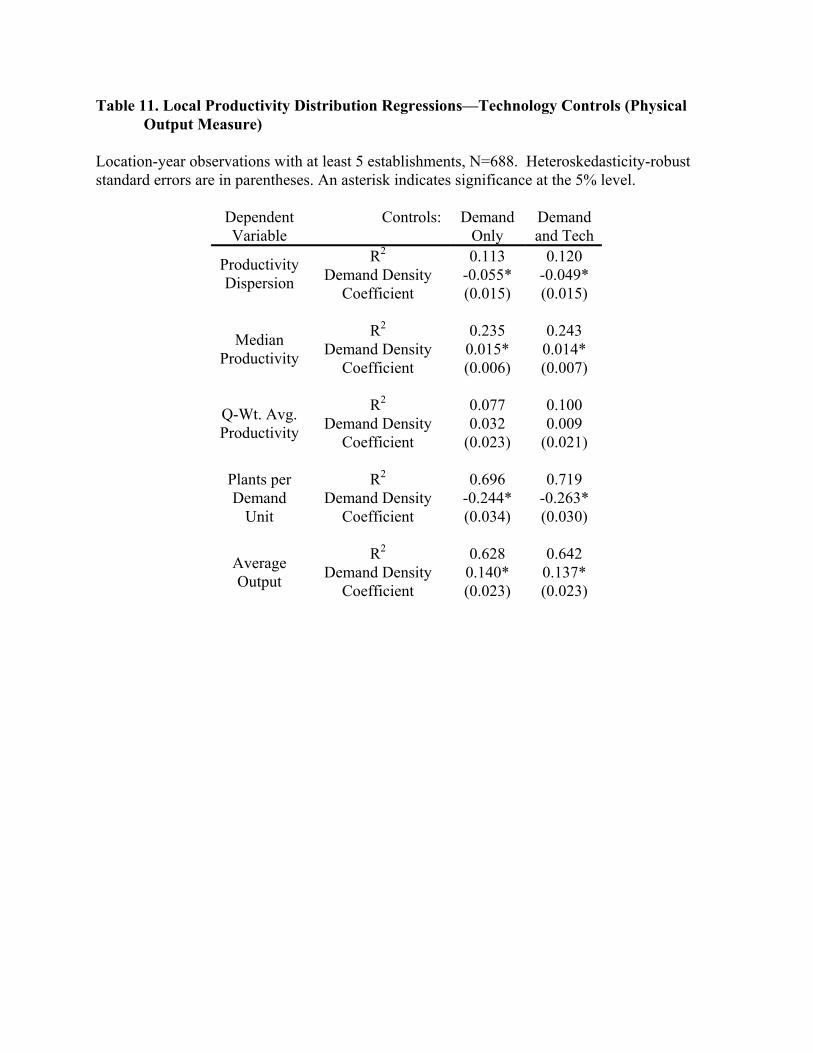
Table 11. Local Productivity Distribution Regressions—Technology Controls (Physical Output Measure)

Location-year observations with at least 5 establishments, N=688. Heteroskedasticity-robust standard errors are in parentheses. An asterisk indicates significance at the 5% level.

Dependent Variable

Controls: Demand Only

Demand and Tech

R2 0.113 0.120 Productivity Dispersion Demand Density

Coefficient -0.055* (0.015)

-0.049* (0.015)

R2 0.235 0.243 Median

Productivity Demand Density Coefficient

0.015* (0.006)

0.014* (0.007)

R2 0.077 0.100 Q-Wt. Avg.

Productivity Demand Density Coefficient

0.032 (0.023)

0.009 (0.021)

R2 0.696 0.719 Plants per

Demand Unit

Demand Density Coefficient

-0.244* (0.034)

-0.263* (0.030)

R2 0.628 0.642 Average

Output Demand Density Coefficient

0.140* (0.023)

0.137* (0.023)