NBER WO~G PAPER SERIES

MARKET SEGMENTATION ANDTHE SOURCES OF RENTS FROM

INNOVATION: PERSONAL COMPUTERS INTHE LATE 1980’S

Timothy F. BresnahanScott Stem

Manuel Trajtenberg

Working Paper 5726

NATIONAL BUREAU OF ECONOMIC RESEARCH1050 Massachusetts Avenue

Cambridge, MA 02138August 1996

We would like to thank seminar participants at Harvard, Princeton, UCLA, Stanford, MIT, theJustice Department, the NBER IO and Productivity Workshops, Econometrics in Tel Aviv 1995, andespecially the Conference in honor of Richard Quandt’s retirement for helpful comments andcriticisms. Cristian Santesteban and Michele Sullivan provided able research assistance. We aregrateful to the Alfred P. Sloan Foundation, to the Technology and Economic Growth Program(Stanford), to the International Center for Research in the Management of Technology (MIT), andto the Stanford Computer Industry Project for support. The research presented, the opinionsexpressed, and any remaining errors are solely those of the authors. This paper is part of NBER’sresearch programs in Industrial Organization and Productivity. Any opinions expressed are thoseof the authors and not those of the National Bureau of Economic Research.

01996 by Timothy F. Bresnahan, Scott Stem and Manuel Trajtenberg. All rights reserved. Shortsections of text, not to exceed two paragraphs, maybe quoted without explicit permission providedthat full credit, including O notice, is given to the source.

Market Segmentation and the Sources of Rents from Innovation:

Personal Computers in the late 1980’s

I. INTRODUCTION

Product innovations contribute to economic progress by expanding the range of choices

available to consumers and by improving the performance dimensions of existing products. However,

the incentives to innovate do not stem directly from the social value of new or improved products

but from the private returns that innovators manage to capture in the marketplace. In order to be

an effmtive inducement, these potential rents must be secured from the competitive threats posed by

pre-existing products, from imitators, and, at least for some time, from products extending the

technological frontier even further. As Arrow (1962) pointed out, innovators have to enjoy some

degree of transitory market power in order to pay for their innovations. In this paper, we examine

some of the critical measurement issues that arise in this context, by evaluating the sources of

transitory market power in the market for microcomputers (commonly referred to as personal

computers, or just PCS) in the late 1980s.

In differentiated, fast changing product markets, innovative firms might be able to take

advantage of several different sources of transitory market power. First, new products might

incorporate novel features, making existing products only an imperfect substitute for the new good.

Second, firms may try to slow down the pace of rent-dissipation in the marketplace by extending the

protective umbrella of a pre-existing brand-name reputation over new product introductions. To take

advantage of this branding, innovators might exploit a widespread willingness to pay a brand

premium; alternatively, the innovator might concentrate on serving high-margin niche markets for the

latest offerings from “high-quality” branded producers (Teece, 1988).

Of course, the classical justification for patents, trademarks, and other forms of formal

intellectual property protection is precisely their ability to provide temporary monopoly power in

order to prompt innovation and creativity; yet, these forms of protection seem to have played only

a minor role in ensuring innovative rents in the PC industry during the late 1980s. ] Consequently, we

1 Patents did not substantially delay the entry of imitators as the indust~ is organized aroundan open technical standard. Thus, our industry is like the majority of those studied by Levin et al.(1987) in the modest role played by patents in ensuring appropriability.

focus here on the role that pushing the technological frontier (in this case meaning the incorporation

of the 80386 microprocessor) and relying on a brand name reputation (such as that of IBM) played

in ensuring transitory market power to innovative PC firms.

Our starting point is the fact that markets for differentiated products often exhibit some form

of segmentation or clustering according to a small number of “principles of differentiation” (PDs).

Each PD defines a distinct notion of product similarity according to the presence or absence of some

key product characteristic and offers a potential source of market segmentation. Thus, products that

belong to the same cluster (defined by these PDs) would be closer substitutes to each other than to

products belonging to other clusters. We consider here two such principles: whether or not the

product is associated with a strong brand name (Branded, B, versus Non-Branded, NB) and whether

or not the product is at the cutting edge of the technological frontier (Frontier, F, versus

Non-Frontier, NF). Both contemporary industry sources as well as retrospective analysis support the

view that the late 1980s market for personal computers indeed exhibited the 4-way clustering implied

by these two PDs: {B, F}, {B, NF), {NB, F}, and {NB, NF}.2 The model of demand that we

estimate, the instruments that we use for that purpose, and the issues that we address with the

estimates all stem from and build upon these two principles of differentiation.

We devote the bulk of the paper to the estimation of a discrete choice model of demand for

PCS that allows us to evaluate the substitution patterns within and across these PDs. To do so, we

draw from and extend recent methodological advances in the empirical study of product differentiated

markets (Bresnahan 1981, 1987; Trajtenberg, 1990; Berry, 1994; Berry, Levinsohn, and Pakes,

1995). Following Berry (1994), we motivate the functional form for the demand system by modeling

a discrete choice maximization problem faced by a set of heterogeneous consumers. We then account

for the potential correlation between price and unobserved quality by utilizing a set of instruments

breed on the attributes of competing products using a model of competition. The specific model that

we put forward, the “Principles of Differentiation (PD) Generalized Extreme Value (GEV),” is a

particular application of the GEV class of models suggested by McFadden (1978). The PD GEV

allows us to treat different potential sources of segmentation symmetrically, thus overcoming the

2 As a matter of semantics, we shall refer to each of these groupings as clu,sters (notice thatPCS belonging to the {NB, NF ) cluster are commonly referred to as “clones”).

2

hierarchical structure (and concomitant limitations) of the familiar Multi-Level Nested Logit model.

Finally, we take advantage of our priors about the prevailing principles of differentiation and use

instrumental variables that reflect “local” (i.e., within-PD) competitive conditions, thus exploiting an

additional source of variation in the context of our short panel dataset.

Our main findings are, first, that the PC market was indeed highly segmented during the late

1980s, along both the F and the B dimensions. Consequently, the effects of competitive events (such

as entry, imitation, or price cuts) in any one cluster were confined mostly to that particular cluster,

with little repercussion on the others. For example, our simulations imply that less than 5% of the

market share achieved by a hypothetical clone entrant would be market-stealing from other clusters.

The second finding is that the product differentiation advantages of B and F were qualitatively quite

different, The advantage associated with positioning a product at the technological frontier was

limited to the relative isolation that it provided from the large number of NF competitors. By

contrast, bestowing a brand name reputation on a new product not only provided some protection

from competition from non-branded PCS, but also s~ed out the product demand curve a great deal.

The paper is organized as follows. In Section 11we discuss some key features of the PC

market in the late 1980s, including sources of buyer heterogeneity and the appropriateness of the

clustering scheme proposed. We then describe the data, consisting of market shares, prices and

attributes for each PC product sold in 1987 and 1988. In Sections IV and V, we develop the

Principle of Differentiation GEV model, review its implementation, and present and discuss the set

of instruments used in the estimation. We present the main results in Section VI, assess their

robustness, and perform some simulations that highlight the extent of segmentation. Section VII

concludes.

3

II. THE PC MARKET IN THE LATE 1980s3

Technical change in personal computing has been extremely fast and sustained; moreover, the

nature of competition among PC fm has changed over time as well. Our snapshot of the market in

1987-88 catches the technology in swift transition with the introduction of a new microprocessor, the

80386, which we associate here with the Frontier, The role played by brand-name reputation is also

highlighted, a role that would evolve and mutate later on, as the identities and types of firms with

substantial brand capital changed. At the time when the 80386 was introduced (in late 1986), the

design and production of microcomputers making effective use of the new chip posed considerable

technical difficulties, and required substantial R&D efforts from PC makers.4 By the end of 1986,

only the most technically capable PC firms had succeeded in introducing an 80386-based system. A

handful of other PC makers would see their development efforts succeed during our sample period,

whereas most other firms took even longer to come out with marketable 386 designs.

A key question posed in this paper is the extent to which PCS that belonged to the Frontier

(or were marketed by a Brand) were insulated from competition by Non-Frontier (Non-Branded)

products. The answer to this question crucially depends on the degree of )leterogeneity among

buyers in their valuation of Frontier andor Branded status. In the presence of substantial

heterogeneity, Frontier (and Brand) can be protected from the competition of Non-Frontier (and

Non-Brand), while at the same time coexisting with these products, neither group eliminating the

other.

3 We limit our analysis ~M PCS and IBM-compatible PCS. Following industry conventionat the time, we exclude both older, 8-bit computers (Apple II, CPM, etc.) and incompatiblearchitectures such as Apple Macintosh. While Macintosh and IBM-compatible machines wouldconverge in capabilities over time (particularly during the early 1990s), there was little importantoverlap among commercial customers during the period under study.

4 By the mid- 1990s, it has become much easier to incorporate frontier technology into PCdesign. This is because a much higher share of PC innovation has become embedded in thecomponents themselves (such as an Intel microprocessor) rather than in the integration amongcomponents (see Henderson and Clark (1990) for a discussion between component-based versusintegration-based innovation). In the era under study in this paper, the opposite was true. PCequipment manufacturers had to develop specialized skills and make substantial expenditures inorder to market a product on the technological frontier (Steffens, 1994).

4

,.

A close-up look at the transition from 286- to 386-based PCS suggests that there were

indeed pronounced differences across buyers in their assessment of the prospective benefits of 386-

ba.sed PCS, From an engineering perspective, the new systems yielded substantial improvements in

the ability to run software due to the increased speed of the microprocessor and an improved address

model for the main memory. However, some users (and analysts) saw 386-based systems just as

faster versions of older PCS. Others, already running or planning to run more advanced and

demanding software (such as the new Microsof~M operating environment, Windows), saw them

as the only sufficient platform that would satisfy their computing needs within the useful life of the

current purchase. These conflicting opinions, echoed in lively debates in the trade press, presumably

led to sigtilcant differences among buyers in their willingness to pay for the much more capable but

also much more expensive 386-based PCS.5 We would expect such heterogeneity to result in a

steeply sloped demand curve for the Frontier PCS, as well as in poor substitutability between Frontier

and Non-Frontier systems. Our model will measure these features of demand, and hence the extent

to which Frontier PCS were insulated from Non-Frontier competition at that time.

PCS differed not only in terms of their technical features, but also in terms of the brand-name

reputation that the manufacturers bestowed on them, During our sample period, PC buyers valued

Brandedness as an indicator of high quality service and support from selling firms, as well as an

indication that the product was reliable and practical for business applications. IBM, the leading brand

name in the PC market for many years, was not just the inventor of the dominant design in PCS but

ako enjoyed a reputation for service, support, and technical excellence from making and marketing

larger computers to business customers. Other large electronics fm also had preexisting reputations;

of these, we treat AT&T and Hewlett Packard as branded based on, (~ their market and

technological leadership in indust~ segments close to PCS; and (ii) their stated commitment to the

business-oriented PC market segment, backed up by substantial advertising and marketing

5 O’Malley (1989) summarized both sides of the debate: “While a 386 or 386SX system oftenis a wiser purchase than a 286, those suggesting the demise of the 286 misunderstand the scopeand diversity of PC applications.”

5

expenditures.b The fourth fm we treat as branded, and the only specialized PC firm so treated, is

Compaq. The largest advertiser in the PC market at the time, Compaq built its brand name by

establishing a reputation for innovation in PCS (such as its introduction of the first 386-based PC

prior to IBM) and by providing reliable service and support for these frontier products (Steffen,

1994). Within a few years after our sample, several other firms built substantial brand reputations

by imitating Compaq’s strategy; however, except for Compaq, none had been successful prior to

1988.7

As with Frontier status, the issue of the degree of insulation from competition that branded

firms enjoyed vis a vis non-branded ones, hinges largely on the extent to which buyers

heterogeneously value the attributes signaled by brandedness. A branded company’s reputation for

service, support, and product reliabtity presumably is valued by all buyers (and we will measure that).

Some buyers, however, may have particularly high valuations for these firm-related attributes, and

presumably will be wiUing to pay an even higher premium for Branded products. In fact, this sort of

heterogeneity was widely reported for PC purchases in our sample period.a Buyers in large

organizations (e.g. those in the Fortune 500) tended to favor branded PCS over those offered by

clone makers. Other, usually smaller, organizations valued brandedness significantly less tending to

buy the cheaper clone computers. In our primary specification, we treat IBM, AT&T, HP and

Compaq as a separate branded group, and seek to measure how insulated their PCS were from

competition from clones.9

b Other large computer companies sold PCS, but primarily to their existing customers ratherthan in a mass market. We treat these, including Burroughs, Honeywell and Wang, as Non-Branded.

7 Dell Computer would be the next entrant into the Branded segment through thedevelopment of a reputation for excellent service and support in conjunction with substantialadvertising.

s See Ryan (1987), Jenkins (1987), and Kolodziej (1988).

9 In related specifications, we also examine whether ~M was further separated from otherbranded firms. We also experiment with the boundary of the branded segment. Other marketingvariables, such as distribution channels (store/mail order) may have been important but do notreceive special treatment in our models.

6

In principle, not just Frontier and Brand but other aspects of PCS, technical and otherwise,

could have been the source of market segmentation and hence of temporary monopoly power.

However, IBM’s historic deeision to have an open architecture for PCS (and the decision of the other

PC fm at the time of our sample to be strictly compatible), allows us to eliminate outright a whole

class of potential sources of market segmentation. IBM’s open architecture meant that buyers could

“mix and match” a wide range of peripherals and add-in cards; therefore, price differentials between

PCS due to such components could be arbitraged away. 10 Given the existence of a competitive retail

market for unbundled components, variations in attributes such as the amount of RAM, or the size

of the hard disk, could not make one PC a poor substitute for another. We therefore treat these

characteristics as hedonic attributes, in the sense that we allow them to shift the relative level of

demand for each PC but not to affect the substitution patterns between products.1 1

Having focused here on the sources of transito~ market power, it is important to put our

sample period in perspective, sketch the forces that brought rapid change to the PC industry, and

transformed time and again the patterns of competition in it. Both the supply of technically advanced

PCS and the demand for desktop computing are being shifted continuously by powerful dynamic

processes. The PC sector itself is technically progressive, Immediately upstream lie other fast-paced,

innovative industries such as integrated circuits, mass storage devices, and so on. The introduction

of ever faster microprocessors, memory chips, and disk drives frequently shifts out the

in~ention-possibilities curve in PCS themselves. There are also a variety of technically progressive

industries downstream. Software products like operating systems, word processors, and spreadsheets

advance rapidly, pushing out the demand for more technical y advanced PCS.

10 Some PCS are limited in the amount of RAM they can maximally hold. Up to this limit,however, buyers can typically populate the computer with more of less RAM according to theirbudget and the software they seek to run. Sellers typically picked these limits so that they did notbind on customers early in the life of the machine.

11 An intermediate case is microprocessor speed, expressed in MHZ. Buyers could notarbitrage it, since speed is “designed into” the microprocessor and controller card. Theavailability of several different processor speeds with most models somewhat mitigated this effectsince, in most cases, buyers could find their ideal point nearly met by an offered variation. Weexamine this issue in a variant of our base specification.

7

These relentless changes mean that both sources of segmentation that we seek to measure,

Frontier and Brand, were shifting rapidly. Shortly after our period, a much larger number of

companies sold 386-based PCS. Later still, newer and faster microprocessors heralded a new frontier.

In the same era, a number of firms improved marketing operations, especially delivery and customer

support, thereby approaching Branded status. In the early 1990s, the principal suppliers of

microprocessors and operating systems, Intel and Microsoft respectively, came to hold much of the

control of PC standards that IBM was losing in our sample period. 12The current PC industry

structure, with multiple technically capable branded firms competing, emerged from these events.

There is little doubt that these changes destroyed much of the transitory market power that we seek

to measure in a moment of transition. However, the private incentives to innovate arise from the

discounted (expected) value of the rents which accrue in each period; in this sense, the period-specific

measurement of transitory market power is a key step towards understanding innovative investment

in dynamic technology-intensive markets.

III. THE DATA

Estimating a product-level differentiated demand system requires data on quantities sold,

prices, and characteristics of each make/model in each year. Estimates of total market size are

also needed. The dataset that we gathered for the present study consists of all PC make/ models

(boxes) for which accurate data on price and attributes could be obtained for 1987 and 1988.

Identifying a comprehensive, well-defined set of distinct make/models constituted a major stumbling

block. Because of the difficulties encountered in gathering accurate data for each and every box, we

restricted the scope of the dataset to those vendors with a relevant market presence (see Table 1).

The resulting sample consists of 121 make/models (observations) for 1987, and 137 for 1988.13

12 During and after our sample period, ~M attempted to regain control of PC marketstandard setting via the 0S/2 operating system and the introduction of a novel (and proprietary)PC design (Micro-Channel Architecture). Ultimately, IBM’s strategy to regain standard settingleadership failed.

13 See Appendix A for a detailed description of the data gathering methodology. Appendix Bprovides precise definitions of all variables used in the analysis.

8

Quantities were obtained from a databme provided by COMTEC Market Analysis Services,

covering the years 1987 and 1988. COMTEC reports in great detail purchases of information

technology (lT) equipment (including PCS) by a large, weighted sample of business establishments

in the U.S.’4 Using COMTEC’S weighting scheme, one can extrapolate from the sample data to

calculate the total number of PCS sold for each make/model, Since COMTEC samples business

establishments in the U.S. whether or not they purchased PCS, one can use the same weighting

scheme to estimate the total potential market size for desktop business PCS. For our purposes we

t~e the potential market to be the total number of office-based employees (39 million.) The model

that we estimate includes an “outside good” (that is, the option of not buying), and therefore

market shares are computed as unit sales of each make/model divided by 39 million,

Our price and characteristics data come from the GML MicroComputer Guide, as well as

from a wide variety of additional sources. We focused on a small number of critical technical

characteristics including the microprocessor, the standard RAM provided (expressed in KB), the

speed (MHZ), and the standard hard disk provided (DISK, in MB). 15

As mentioned above, our analysis relies heavily on the possible existence of two

principles of differentiation in the PC market at the time: whether or not the PC was at the

technological frontier and whether or not it was produced by a branded firm. We capture the former

with a dummy variable (FRONTIER) that assigns the value of 1 to PCS incorporating the 80386

microprocessor, and O to those with all other microprocessors (the 286, 8088, and older). As

mentioned in Section II, we identified four vendors for which a brand name was a potentially

import ant determinant of demand and substitution patterns: IBM, AT&T, Hewlett-Packard and

Compaq. 16 The variable BRANDED assigns 1 to products produced by these four firms and O to

14 The COMTEC “Wave 6“ dataset that we use here is based on a sample of over 6,000establishments. Note that the sample excludes households.

15 These are the characteristics actually used in the estimation. We also collectedinformation on the monitor type (B&W or Color), whether the machine was portable, modelvintage, etc.

16 Other configurations were attempted; the qualitative results are not affected by theinclusion or exclusion of branded firms at the margin.

9

products produced by other vendors,

Tables 2-4 provide a useful portrait of the PC industry in each of the years under study.

Though the two samples are only a year apart, there are substantial differences in the average

price/performance of PCS sold. Whereas the average price changed only slightly between the two

years ($3,225 to $3,205), the average hard disk size (DISK), speed (MHZ), and memory (RAM)

all increased substantially. For example, the average standard RAM increased from 611 KB to

688 KB. Indeed, the average level of each of these characteristics rose over 10% between the

two years. The rate of technical advance is accentuated if the observations are weighted by the

quantities sold. For example, the weighted average standard RAM rises from 584 KB to716 KB.

The rate of advance shows also in the share of 386-based PCS (i.e., the average for FRONTER),

which grew from 10% of the sample in 1987 to 1570 in 1988. By contrast, the number of

BRANDED products stayed nearly constant, averaging 30% of the number of make/models

marketed in both years. The advance in the price/performance ratio is highlighted in a regression of

price on the observed product characteristics (Table 3). The coefficients for each of the technical

characteristics are estimated to be positive, while the 1988 coefficient is substantially lower than for

1987. While a substantial amo~nt of price variation exists in each year, our sample reflects the rapidly

falling real prices for computing power which has characterized this market segment since its

inception (Bemdt and Griliches, 1993).

Finally, we “slice” the data according to our PDs (Branded and Frontier) in Table 4. Perhaps

the most striking statistic from this table is that while a relatively high share of all products are

concentrated in the NB~F cluster, at least 6090 of the boxes sold in each year are drawn from the

B/NF cluster. Moreover, the average price for boxes rises as one moves from the “clone” NB/NF

cluster through NBF (or B/NF), with the highest average prices in the BE cluster. While this

preliminary cut of the data suggests the presence of substantial returns to membership in either the

F or B group, one cannot identify the precise way in which these returns manifested themselves

(through the benefit of a large demand curve, or, alternatively, a steep one) from this simple table.

Instead, our more systematic evaluation of the returns to membership in the B or F group will follow

the estimation of the differentiated product demand system, the model to which we now turn.

10

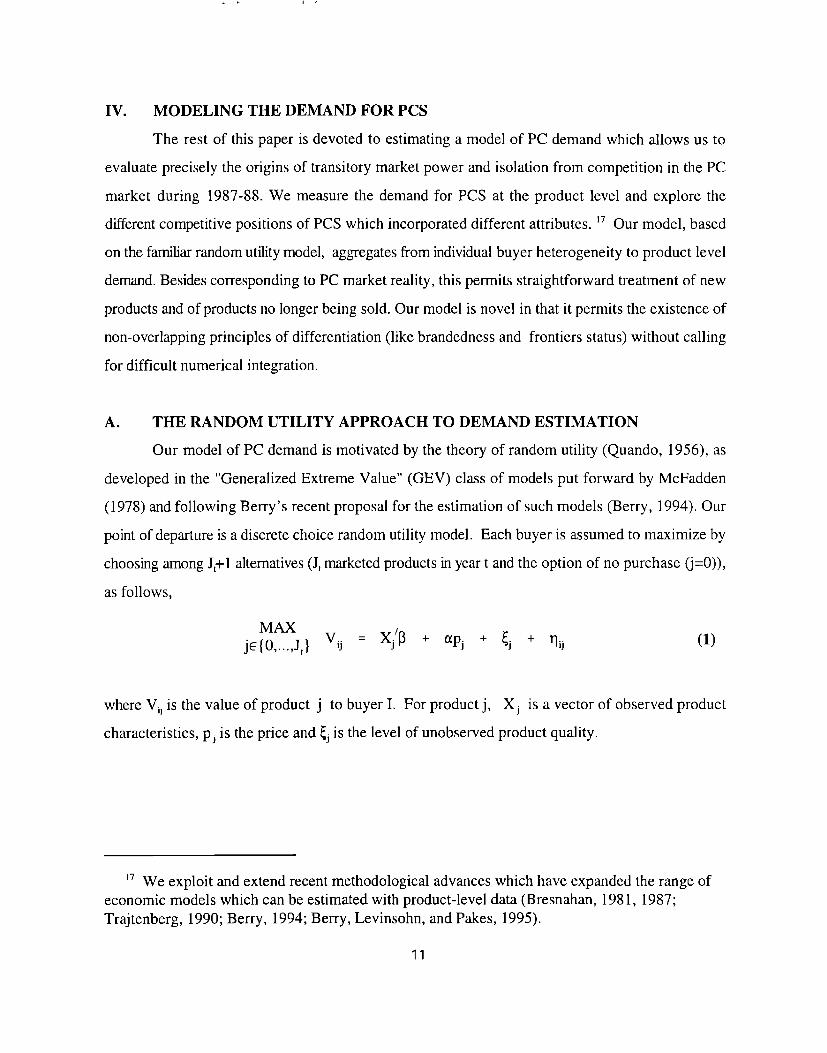
IV. MODELING THE DEMAND FOR PCS

The rest of this paper is devoted to estimating a model of PC demand which allows us to

evaluate precisely the origins of transitory market power and isolation from competition in the PC

market during 1987-88. We measure the demand for PCS at the product level and explore the

different competitive positions of PCS which incorporated different attributes. 17 Our model, based

on the familiar random utility model, aggregates from individual buyer heterogeneity to product level

demand. Besides corresponding to PC market reality, this permits straightforward treatment of new

products and of products no longer being sold. Our model is novel in that it permits the existence of

non-overlapping principles of differentiation (like brandedness and frontiers status) without calling

for difficult numerical integration.

A. THE RANDOM UTILITY APPROACH TO DEMAND ESTIMATION

Our model of PC demand is motivated by the theory of random utility (Quando, 1956), as

developed in the “Generalized Extreme Value” (GEV) class of models put forward by McFadden

(1978) and following Berry’s recent proposal for the estimation of such models (Berry, 1994). Our

point of departure is a discrete choice random utility model. Each buyer is assumed to maximize by

choosing among J,+l alternatives (J[marketed products in year t and the option of no purchase (j=O)),

as follows,

MAX

j~{O,...,J,)Vij = Xj’p + apj + gj + Tlij (1)

where Vi is the value of product j to buyer 1. For product j, X j is a vector of observed product

characteristics, p j is the price and ~j is the level of unobsemed product quality.

‘7 We exploit and extend recent methodological advances which have expanded the range ofeconomic models which can be estimated with product-level data (Bresnahan, 1981, 1987;Trajtenberg, 1990; Berry, 1994; Berry, Levinsohn, and Pakes, 1995).

11

,.

Our treatment follows Berry (1994), decomposing Vi into t-.voparts. Let

aj = X;p + ap. + g.J J (2)

be the mean valuatio n by buyers for product j. Thus, qi is the difference between buyer I’s value for

product j from the average valuation in the population (~j). Each buyer receives a draw of the J,+l

vector, q,, which is a realization of the random variable q. The draws are independent across buyers

but a given buyers’ draw of qti need not be independent of qk if products j and k share

similar product characteristics. The distribution of q depends on parameters p and the product

characteristics X. We write this (J+ 1 dimensional) CDF as F(q; X, p). Thus, {~, a, p } is the vector

of parameters to be estimated in this discrete choice demand system.

Since the work of Quandt (1956), we have known that the distribution of the random shocks

to valuation, here q, is a key determinant of the shape of demand. In the context of our discrete

choice model, there is in fact a precise relationship between the distribution of q at the individual

buyer level and the pattern of cross-product elasticities at the aggregate market level. The modeler

picks a family of distributions F(q; X, p). Particular values of the parameter vector p correspond

to patterns of dependence in q across products sharing common (or similar) product characteristics.

Our model contains a parameter p~, for example, which permits dependence across the idiosyncratic

shocks to Frontier products. For certain values of p~, a buyer strongly prefening any Frontier

product (qij >> O) is also likely to strongly prefer all Frontier products (E [qk I qti >> O] >>0]

if k and j share Frontier status.)

Now consider the impact of an increase in the price of particular product j: the value of

product j falls (at a rate a) and some portion of those consumers whom had initially chosen j are

induced to switch to what had been previously their second-best alternatives. Because of the

dependence in the distribution of q, a relatively high share of these second-best alternatives will be

other Frontier products. More generally, positive dependence in the distribution of q among similar

products makes those products closer substitutes.]a The parameters p measure that dependence.

‘8 This type of dependence across observations can be contrasted with the case where q is iidacross choices (as in the multinominal logit). Under the assumption of independence, the

12

As dependence in q across products with similar products characteristics b.comes stronger,

competition will become more “segmented,” in the sense that the impact of competitive events (such

as a price decrease or entry) will be confined mostly to those products with similar characteristics.

In other words, in this framework a model of which classes of products are close substitutes & a

model of dependence among the elements of q related to product characteristics.

B. A PRINCIPLES OF DIFFERENTIATION GEV MODEL OF PC DEMAND

Of course, a separate question exists m to how to ident~ those product characteristics which

may be important for understanding differentiation and market segmentation. Fortunately, economic

theory, in conjunction with an understanding of the particular market under study, provides

considerable guidance. Like many other consumer products, there exists several features of the PC

(such as the amount of RAM or the size of the hard drive) for which there exists a separate market

for that feature (or component). In the presence of competitive component markets, buyers will

arbitrage away price premiums msociated with the incorporation of these components into particular

products. In other words, to the extent that consumers can “repackage” products along a specific

dimension, each consumer will equate their m~ginal utility for this dimension to its price in the post-

sales market. Accordingly, there wiUk no ex-post heterogeneity among consumers in their marginal

valuations for this dimension. Thus, in choosing how to parametrize the distribution function F(q;

X, p), one should incorporate potential correlation among products which share characteristics which

are not “repackageable,”

Guided by this rule, we focus on two product characteristics which we argue are not

repackageable -- Branded and Frontier. The existence of a Brand name reputation, by construction,

cannot be marketed in the post-sales market. As well, during the period under study, considerable

technical expertise was required to incorporate the 80386 microprocessor into a PC. In contrast,

buyers could entertain several post-sales options to recotilgure their memory options (e.g., RAM and

DISK) and, to a lesser extent, the speed of their microprocessor (MHZ).

introduction of a new product will have the same (proportional) effect on all products in themarket, regardless of characteristics. This implication of the iid assumption is just a restatementof the “Red Bus/Blue Bus” problem emphasized by McFadden (1973).

13

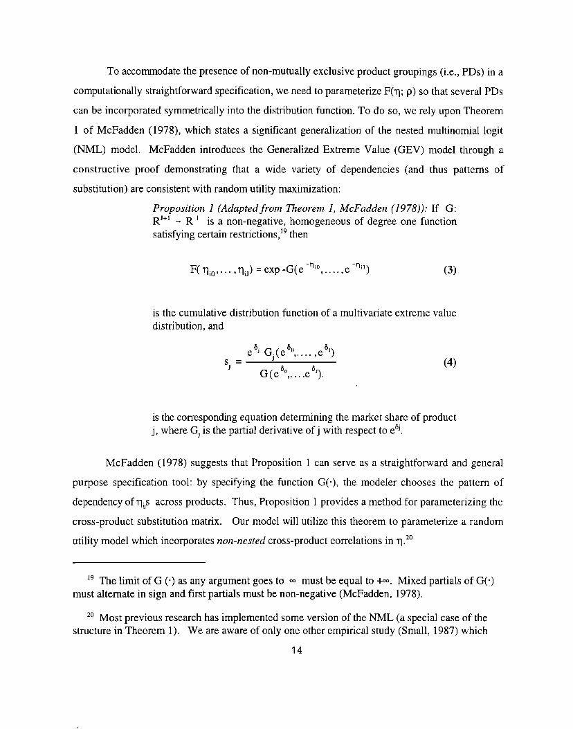
To accommodate the presence of non-mutually exclusive product groupings (i.e., PDs) in a

computationally straightforward specification, we need to parametrize F(q; p) so that several PDs

can be incorporated symmetrically into the distribution function. To do so, we rely upon Theorem

1 of McFadden (1978), which states a significant generalization of the nested

(NML) model. McFadden introduces the Generalized Extreme Value (GEV)

constructive proof demonstrating that a wide variety of dependencies (and

substitution) are consistent with random utility maximization:

multinominal logit

model through a

thus patterns of

Proposition 1 (Adaptedfrom Theorem 1, McFadden (1978)): If G:RJ+l _ R 1 is a non-negative, homogeneous of degree one functionsatisfying certain restrictions,19 then

F(qio,... ,qiJ) =exp-G(e -nio,. . ..ni-)i’) (3)

is the cumulative distribution function of a multivariate extreme valuedistribution, and

ebj Gj(e6(’, . . . . , e b’)Sj =

G(e6(’,,...e5J).(4)

is the corresponding equation determining the market share of productj, where G, is the partial derivative of j with respect to e8J.

McFadden (1978) suggests that Proposition 1 can serve as a straightforward and general

purpose specification tool: by specifying the function G(s), the modeler chooses the pattern of

dependency of qfis across products. Thus, Proposition 1 provides a method for parameterizing the

cross-product substitution matrix. Our model will utilize this theorem to parametrize a random

utility model which incorporates non-nested cross-product correlations in q .20

19 The limit of G (.) as any argument goes to OJ must be equal to +~. Mixed partials of G(.)must alternate in sign and first partials must be non-negative (McFadden, 1978).

20 Most previous research has implemented some version of the NML (a special case of thestructure in Theorem 1). We are aware of only one other empirical study (Small, 1987) which

14

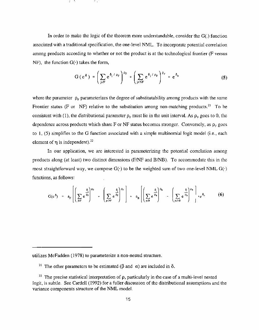
In order to make the logic of the theorem more understandable, consider the G(.) function

msociated with a traditional specification, the one-level NML. To incorporate potential correlation

among products according to whether or not the product is at the technological frontier (F versus

NF), the function G(”) takes the form,

[F )p’+[j~e’’’)p)+e+(’(’G(e*) =~e*J’pF (5)

where the parameter p~ parameterizes the degree of substitutability among products with the same

Frontier status (F or NF) relative to the substitution among non-matching products .21 To be

consistent with (1), the distributional parameter p~ must lie in the unit interval. As p~ goes to O, the

dependence across products which share For NF status becomes stronger. Conversely, as p~ goes

to 1, (5) simplifies to the G function associated with a simple multinornial logit model (i.e., each

element of q is independent) .22

In our application, we are interested in parameterizing the potential correlation among

products along (at least) two distinct dimensions (F/NF and B/NB). To accommodate this in the

most straightforward way, we compose G(.) to be the weighted sum of two one-level NML G(o)

functions, as follows:

G(e *) = a~[[2:1” + [Le+l%

+ aB

utilizes McFadden (1978) to parametrize a non-nested structure.

21 The other parameters to be estimated (~ and a) are included in 5.

(6)

22 The precise statistical interpretation of p, particularly in the case of a multi-level nestedlogit, is subtle. See Cardell (1992) for a fuller discussion of the distributional assumptions and thevariance components structure of the NML model.

15

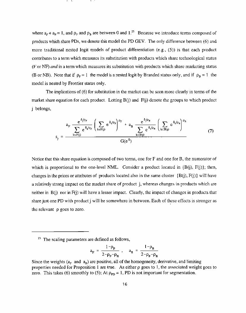
where a~+ a~= 1, and p~ and p~ are between 0 and 1.23 Because we introduce terms composed of

products which share PDs, we denote this model the PD GEV. The only difference between (6) and

more traditional nested logit models of product differentiation (e.g., (5)) is that each product

contributes to a term which memures its substitution with products which share technological status

(For NF) and in a term which measures its substitution with products which share marketing status

(B or NB). Note that if pp = 1 the model is a nested logit by Branded status only, and if p, = 1 the

model is nested by Frontier status only.

The implications of(6) for substitution in the market can be seen more clearly in terms of the

market share equation for each product. Letting BQ) and Ffi) denote the groups to which product

j belongs,

(7)~e’(j)

G(ea)

Notice that this share equation is composed of two terms, one for F and one for B, the numerator of

which is proportional to the one-level NML. Consider a product located in {B~), Ffi) }; then,

changes in the prices or attributes of products located also in the same cluster {B~), F(j) } will have

a relatively strong impact on the market share of product j, whereas changes in products which are

neither in B(j) nor in F~) will have a lesser impact. Clearly, the impact of changes in products that

share just one PD with product j will be somewhere in between. Each of these effects is stronger as

the relevant p goes to zero.

23 The scaling parameters are defined as follows,

1-pF 1-p’aF =

2-pF-pB ‘aB =

2-PF-PB

Since the weights (a~ and a~) are positive, all of the homogeneity, derivative, and limitingproperties needed for Proposition 1 are true. As either p goes to 1, the associated weight goes to

zero. This takes (6) smoothly to (5); At ppD= 1, PD is not important for segmentation.

16

While our proposed model, (6), is quite simple, Proposition 1 can accommodate a wide range

of different clustering structures, including a larger number of “principles of differentiation, ”

interactions between them, etc. Incorporating additional dimensions of potential product

differentiation simply requires adding suitable terms to (6).24 In this sense, the McFadden Theorem

provides a useful and underutilized modeling tool with potentially wide applicability.

c. THE PD GEV VERSUS ALTERNATIVE MODELS OF SUBSTITUTION

Given our goal to measure the degree of segmentation afforded by (at least) two distinct PD’s

(B/NB and F/NF), several issues arise which make the most traditional (and computationally

straightforward) parameterizations of the joint distribution of q inappropriate for our problem. First,

because we want to distinguish between several different sources of product differentiation, we

cannot employ a simple unidimensional vertical product differentiation (VPD) specification

(Bresnahan, 1981, 1987; Berry, Camall and Spiller, 1996; Stavins, 1996), in which a single

distributional parameter measures variation among consumers in their preferences for overall product

quality. As well, a nested multinominallogit (NML) model (Trajtenberg, 1990; Goldberg, 1995; Stem,

1996), in which several mutually exclusive dimensions of product differentiation can be incorporated,

is also inappropriate. For example, if we were to specify (1) to be a two-level nested logit with the

top level of the nesting determined by the B/NB distinction (Figure 1), we would be assuming away

potential correlation in q (and the resulting implications for market-level substitution) among

products which share Frontier status but do not match along the B/NB dimension. Thus, neither the

VPD and W models can parametrize our principal hypotheses directly -- the separate existence

of segmentation along two overlapping dimensions (F/NF and B/NB).

In order to assess the relative merits of the PD GEV, it is worth comparing it in more detail

to the two-level M (see Figure 1). It is important to note that our proposed model (6) is no more

richly parameterized than a two-level NML. Instead, the difference between the two models is that

the PD GEV accommodates substitution in a way that we argue is more appropriate for our

24 We have estimated several variant models (only a subset of which are presented in theResults Section). We have experimented with additional clustering by MHZ (as in Small ,1987),an “IBM” cluster, as well as others.

17

application. In particular, while in both models products sharing both B and F status are closer

substitutes to each other than to other prodL~cts, the models differ in their treatment of substitution

among the partially matching products (note that the groups in the PD GEV are not mutually

exclusive).

Consider the two-level NML (with B on top) in the upper panel of Figure 1: the parameter

p~ determines how much “closer” products sharing both B and F are than those sharing only B. In

this sense, the NML is parameterizing segmentation along more than one dimension. However,

lowering the price of a {B, F} product hm the same effect on market shares in the partially matching

(NB, F) category as in the completely unhatching {NB, NF] category.” In this sense, the NML

permits only one of the two partially matching clusters to be close substitutes. Moreover, reversing

the order of nesting just reverses the problem.2b

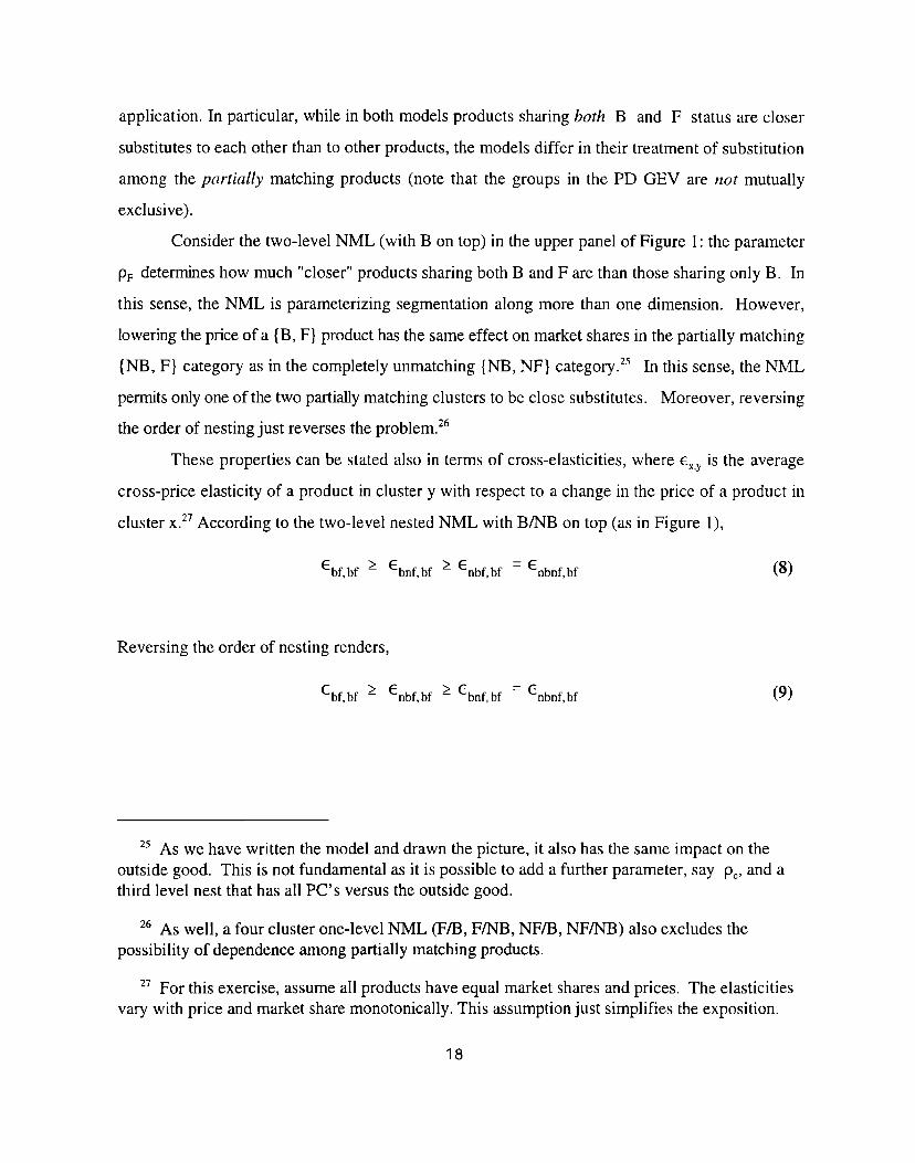
These properties can be stated also in terms of cross-elasticities, where ~X,Yis the average

cross-price elasticity of a product in cluster y with respect to a change in the price of a product in

cluster x 27According to the two-level nested NML with B~B on top (as in Figure 1),

Reversing the order of nesting renders,

E~fbf 2 E“bf ~f 2 Ebnf ~f = enbnf ~f

(8)

(9)

25 As we have written the model and drawn the picture, it also has the same impact on theoutside good. This is not fundamental as it is possible to add a further parameter, say pC,and athird level nest that has all PC’s versus the outside good.

26 As well, a four cluster one-level NML (F/B, F~B, NF/B, NFNB) also excludes thepossibility of dependence among partially matching products.

27 For this exercise, assume all products have equal market shares and prices. The elasticitiesvary with price and market share monotonically. This assumption just simplifies the exposition.

18

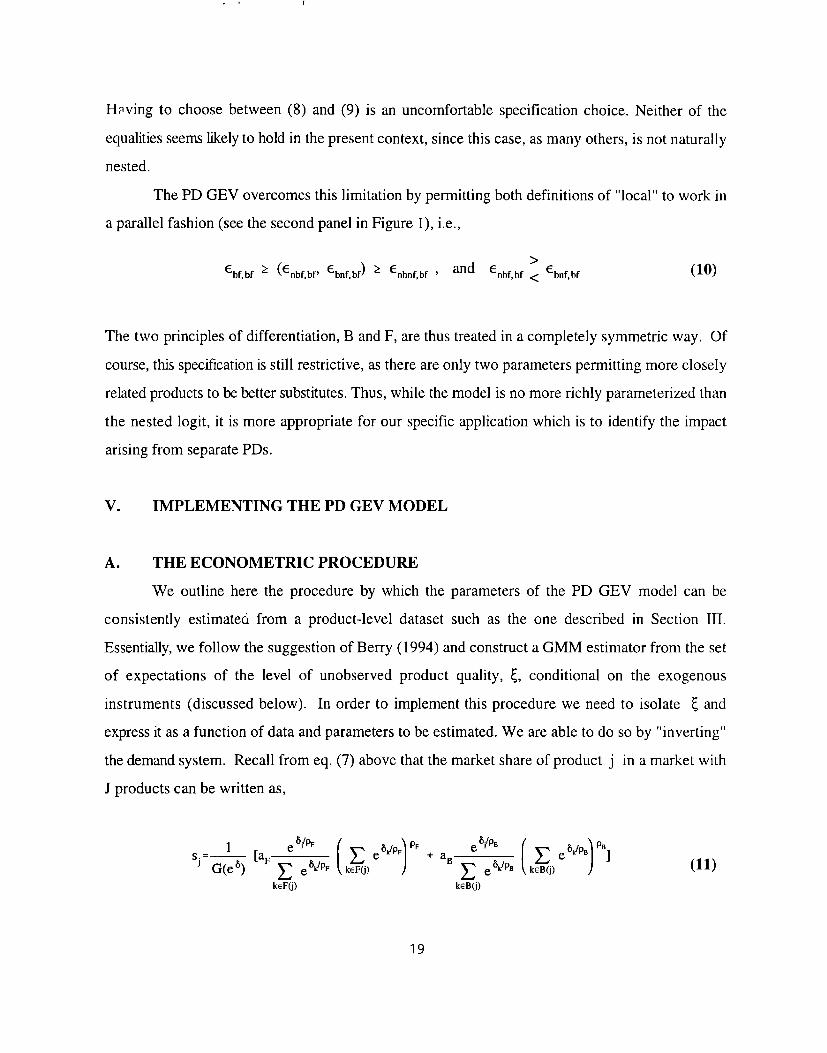
H~ving to choose between (8) and (9) is an uncomfortable specification choice. Neither of the

equalities seems likely to hold in the present context, since this case, as many others, is not naturally

nested.

The PD GEV overcomes this limitation by permitting both definitions of “local” to work in

a parallel fashion (see the second panel in Figure 1), i.e.,

E bf, bf 2 (E nbf, bf’ ‘bnf,bf) 2 ‘n~nf,bf ! and ‘nbf,bf ~ ‘bnf, bf (lo)

The two principles of differentiation, B and F, are thus treated in a completely symmetric way, Of

course, this specflcation is still restrictive, as there are only two parameters permitting more closely

related products to be better substitutes. Thus, while the model is no more richly parameterized than

the nested logit, it is more appropriate for our specific application which is to identify the impact

arising from separate PDs.

v. IMPLEMENTING THE PD GEV MODEL

A. THE ECONOMETRIC PROCEDURE

We outline here the procedure by which the parameters of the PD GEV model can be

consistently estimated from a product-level dataset such as the one described in Section III.

Essentially, we follow the suggestion of Berry (1994) and construct a GMM estimator from the set

of expectations of the level of unobserved product quality, ~, conditional on the exogenous

instruments (discussed below). In order to implement this procedure we need to isolate ~ and

express it as a function of data and parameters to be estimated. We are able to do so by “inverting”

the demand system. Recall from eq. (7) above that the market share of product j in a market with

J products can be written as,

(11)

19

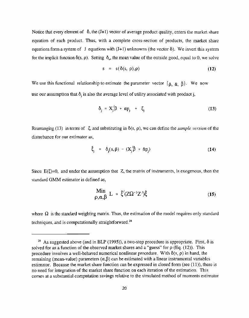
Notice that every element of 8, the (J+l) vector of average product quality, enters the market share

equation of each product. Thus, with a complete cross-section of products, the market share

equations form a system of J equations with (J+ 1) unknowns (the vector 5). We invert this system

for the implicit function 6(s, p). Setting 8., the mean value of the outside good, equal to O, we solve

s= S(a(s, p), p) (12)

We use this functional relationship to estimate the parameter vector {~, h, ?). We now

use our assumption that ~j is also the average level of utility associated with product j,

bj = Xj’p + ap. + g.J J

(13)

Rearranging (13) in terms of ~, and substituting in 5(s, p), we can define the sa~nple ~’ersiotzof the

disturbance for our estimator as,

(14)

Since E(~)=O, and under the assumption that Z, the matrix of instruments, is exogenous, then the

standard GMM estimator is defined as,

‘in L = ~’(ZQ-lZ ‘)~p,a,p

(15)

where Q is the standard weighting matrix. Thus, the estimation of the model requires only standard

techniques, and is computationally straightforward.28

2s As suggested above (and in BLP ( 1995)), a two-step procedure is appropriate. First, 5 issolved for as a function of the observed market shares and a “guess” for p (Eq. (12)). Thisprocedure involves a well-behaved numerical nonlinear procedure. With 6(s, p) in hand, theremaining (mean-value) parameters (a, ~) can be estimated with a linear instrumental variablesestimator. Because the market share function can be expressed in closed form (see (11)), there isno need for integration of the market share function on each iteration of the estimation. Thiscomes at a substantial computation savings relative to the simulated method of moments estimator

20

1.

B. INSTRUMENTS

The GMM estimator in (15) requires an instrumental variables (IV) vector, Z, with rank at

least as large as the dimensionality of the parameter vector, {~, a, p}. Of course, the efficient IV

vector is composed of the derivatives of the disturbance (t) with respect to the parameters. In the

current application it is quite difficult to construct the optimal Z, so we propose a simpler strategy

for the construction of Z for PD GEV models.

Our strategy relies on the econometric erogeneity of the entire matrix of product

characteristics, X. In the spirit of the recent literature, we use a model of supply to point out

functions of X which make plausible instruments. 29A row of our proposed Z(X) consists of

Xj, the observed product characteristics of product j

counts and means of X for products sharing a cluster with product j

. counts and means of X for products sold by the firm offering product j

counts and means of X for products sharing both cluster and seller.

This section first visits the general econometrics issues briefly. We then explain how our IV strategy

follows from an assumption of equilibrium pricing behavior by sellers in an industry with PD GEV

demand.

We face two challenges in constructing Z. With market power on the supply side, it is

dfilcult to just~ an assumption that price is independent of t; c has the interpretation of unobserved

product quality, meaning that a higher c, should lead suppliers to set a higher p. As a result,

E(P~)>0,30 Similar arguments mean that the prices and share of other products are correlated with

~J,so that the first term as well as the last term in the RHS of (14) calls for IV. To make this more

implemented in BLP (1995), Additional information (including GAUSS estimation programs) areavailable by public access ftp archive.

29Our approach is most like of BLP ( 1995), who impose some of the economic restrictions oftheir model on Z(X). Unlike BLP, we offer no proof that our Z is the first under term in a seriesapproximation to the optimal IV.

30 This problem was emphasized by Trajtenberg (1989, 1990), who found that the demand forCT scanners was estimated to be positively sloped in the context of an NML model withexogenous prices. Further analysis revealed that omitted quality, correlated with price, was indeedthe culprit for the positive bias. Our solution follows Berry (1994).

21

.“ ,

difficult, the econometric framework is inherently nonlinear.31 In the face of such nonlinearity (and

without additional assumptions), the efficient IV vector will contain elements which are themselves

functions of the parameters to be estimated, leading to substantial computational difficulties

(Chamberlain, 1987).

In response to the difficulties, we propose to utilize our assumption that X, the matrix of

observed product characteristics in year t, is exogenous. The immediate implication of this

assumption is that we are able to include Xjdirectly in Z. This immediately reduces the number of

excluded instruments needed to dim (a,p ). ‘2

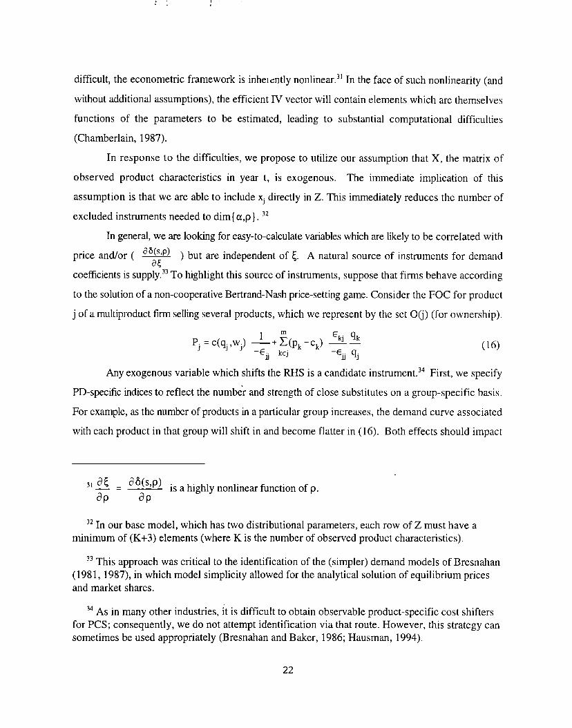
In general, we are looking for easy-to-calculate variables which are likely to be correlated with

price and/or ( * ) but are independent of ~. A natural source of instruments for demand

coefficients is supply .33To highlight this source of instruments, suppose that firms behave according

to the solution of a non-cooperative Bertrand-Nash price-setting game. Consider the FOC for product

j of a multiproduct fm selling several products, which we represent by the set 0~) (for ownership).

(16)

Any exogenous variable which shifts the RHS is a candidate instrument.34 First, we specify

PD-specific indices to reflect the number and strength of close substitutes on a group-specific basis.

For example, as the number of products in a particular group increases, the demand curve associated

with each product in that group will shift in and become flatter in (16). Both effects should impact

-j, at aa(s,p)—= is a highly nonlinear function of p.ap ap

32In our base model, which has two distributional parameters, each row of Z must have aminimum of (K+3) elements (where K is the number of observed product characteristics).

33This approach was critical to the identification of the (simpler) demand models of Bresnahan(1981, 1987), in which model simplicity allowed for the analytical solution of equilibrium pricesand market shares.

‘4 As in many other industries, it is difficult to obtain observable product-specific cost shiftersfor PCS; consequently, we do not attempt identification via that route. However, this strategy cansometimes be used appropriately (Bresnahan and Baker, 1986; Hausman, 1994).

22

the observed price and the product’s within-group market “hare. Thus, the number of products in

each group will be correlated with the impact of the segmentation parameters, a and p, on prices and

the implicit function 5(s,p). Essentially, we exploit our assumption that the group-specific entry

process is exogenous (in an econometric sense) to create a “local” index of the number of substitutes

for each product. As shown in Table 5, we implement this idea by calculating an instrument vector

for observation j which includes the number of products in F~) and B~), the groups to which product

j belongs, as well as sums over the characteristics of other products in FQ) and B(j).

We also calculate “Ownership” instruments (Iabelled so in Table 5) which exploit the

economics of multiproduct pricing as reflected in the RHS of (16). For example, as a particular firm

sells a larger share of the number of total products available, it will charge a higher price on each

product (as compared to the prices which would be observed under a more unconcentrated market

structure). Similarly, the sum of the characteristics of the products of the firm (other than j) will be

positively correlated with price, since that

two analytical arguments and use the

ownership and cluster.

By using PD-spec~lc instruments,

would mean higher q~ in eq.( 16).s5 Finally, we blend these

characteristics and count of products which share both

we use somewhat different instruments than our immediate

predecessors in the literature (BLP (1995)). In particular, we are using our assumption about the

group structure of product differentiation to construct the excluded IVS. This strategy is successful

because some groups, like Frontier, saw much more entry than others. This entry, which we assume

to be exogenous, shifts prices and maket shares by changing competition. The different rates of entry

across groups means that our proposed instruments vary even in the short panel considered in the

present application. It is useful to note that our erogeneity assumption may not be as strong as it

seems at first blush. In particular, while we believe that entry into specific clusters is endogenously

determined by its economic returns, this does not mean that our instruments are correlated with the

error. We include dummies for both B and F in observable product quality; which means that ~ is

merely the deviation of the products’ quality from the cluster means.

Finally, the discussion so far has been predicated on the assumption that firms engage in

35 In this argument we closely follow BLP (1995).

23

Bertrand competition. However, if firms play a different type of non-cooperative game (e.g.

Coumot), then the precise form of (16) would change, but our instruments would be unaffected, since

the logic of ownership-based and group-based instruments remains the same. Outright collusion

though would make a difference, since ownership-based instruments would be longer be relevant.

More generally, the point is that the instruments should reflect the underlying supply and demand

conditions that prevail in the market, that is, the type of price setting behavior of firms, and the nature

of the heterogeneity of consumers as manifested in the groups. For the case at hand, we assume that

firms used individualistic pricing strategies; the pace of technical change in PCS and the ensuing

intensity of competition seems to have prevented price collusion, However, we will explore the

importance of this assumption by removing the ownership-based and PD-based instruments from Z

in the course of evaluating the robustness of our results.

VI. RESULTS

We turn now to the presentation and analysis of results from the estimation of the PD GEV

for a variety of specifications. We also present estimates of alternative Two-Level NML and VPD

models and contrast them with the PD GEV. After exploring the robustness and limitations of the

model, we illustrate the meaning of the estimates by drawing hypothetical demand functions for

Branded and Frontier PCS and perform a set of counterfactuals involving hypothetical entry to

highlight the high degree of market segmentation that these estimates imply.

A. PRINCIPAL FINDINGS

We frst preview our main findings (drawn from Model 1 in Table 6) in a concise fashion to

help frame the discussion of the results:

(I) 0< (p,, p,) <<1. Both of the substitution parameters areestimatedto be small (significantly

smaller than 1), suggesting that there is indeed a high degree of market segmentation along both the

B and F dimensions: Non-Branded products are poor substitutes for Branded products and

Non-Frontier products are poor substitutes for Frontier products. The parameter p~ is estimated

quite precisely in most specifications, while the estimate of p~ is much less precise. Nevertheless,

the estimates for both distributional parameters are quite stable across specifications.

24

(ii) The product differentiation advantages of B and F are different. The advantage of being at the

frontier is limited to the insulation it provides from NF competition (p~eel). Perhaps surprisingly,

incorporating Frontier technology dld not necessarily shift the product demand curve out (~~~OmI~~

is small, usually negative, and always imprecisely estimated). In contrast, having a brand name shifts

out the product demand curve (~~m > O) and provides B products with some protection from NB

competition (p~ < 1),

(iiz] As expected, the price coefficient, a, is sensitive to whether or not the model accounts for price

endogeneity, and to the type of instruments used. Models that ignore the correlation of price with

unobserved quality result in much smaller (in absolute value) estimates of a; models which do not

exploit the full set of proposed instruments severely reduce the precision of this estimate.

(iv) The choice of model specification turns out indeed to be important for analyzing the market under

study. In fact, the leading alternative to the PD GEV model, the Two-Level NML, yields estimates

that are highly sensitive to the order of nesting. In particular, the relative sizes and significance of the

substitution parameters are reversed in the Two-Level NML model with the B/NB nest on top, vis

a vis the one with the F/NF nest on top. Thus, the PD GEV model offers an attractive method~logical

alternative, at least in those cases where the nesting order is not well defined a priori.

B. MAIN SPECIFICATION, ROBUSTNESS AND IDENTIFICATION

We present in Table 6 our base specification (Model 1), two alternative specifications in

which we vary the elements of X (the set of product characteristics), and a fourth one where we add

an additional PD. The parameters estimated are the distributional coefficients p~ and p~, a price

coefficient, a , various ~s (a constant, and coefficients for FRONTIER, BRANDED, IBM, and for

a sub-set of DISK, RAM, and MHZ), as well as p~~z in Model 4.

As previewed above, the estimates of p~ and p~ are quite small in all these specifications.

In fact, even though p~ is estimated very imprecisely, one can easily reject the hypotheses that p~ =

1 and/or p~ = 1. The results for the price coefficient, a, are encouraging: it is estimated to be

negative and quite stable across specflcations; however, its level of significance varies quite a bit (fair

25

in Models 1 and 2, nil in Models 3 and 4). In all four models, the BRANDED coefficient is large,

positive, and significant while the FRONTIER coefficient cannot be distinguished from zero (and is

in fact negative in three out of four specifications). The ~M coefficient is positive and gives (at the

point estimate in the b~e specflcation) a 50% incremental boost to IBM products above and beyond

other Branded products. Finally, our technological control variables (DISK, RAM, and MHZ) have

the expected sign, though only the DISK coefficient is significant (in Model 1).36

It should be noted that the coefficients that determine the level and slope associated with B

and F, which are of particular interest here, are relatively stable across the four specifications.

Moreover, the point estimates suggest that there was a qualitative difference in the product

differentiation advantage afforded along the F versus the B dimension. In fact, we are able to reject

the hypothesis:

HO: p~ = p~, PF = ~B

at the 90% level in our main spec~lcation (Wald test statistic = 5.22, X2(OW,z, = 4.61). While the high

standard errors of the F coefficients do not allow us to draw firm conclusions (e.g., we cannot reject

~ at the 95% level), a cautious interpretation of this result is that, relative to the advantages arising

from having a brand name, being at the Frontier proved to be beneficial more in the sense of insulating

from competition than in pushing out the demand curve. In Model 4 we include a MHZ substitution

parameter (p~Hz = .99).37 In contrast to the substantial segmentation found along both the B and F

dimensions, there seems to be little evidence that there existed segmentation along the MHZ

dimension (we cannot reject HO: p~~z = 1).

In Table 7, we compare the estimates from the PD GEV with those from two alternative

spec~lcations of the Two-Level NML model. The most troubling feature of Models 5 and 6 is the

high sensitivity of the estimates to the order of nesting. In particular, with B/NB on top, p~ << pF,

36 We tried also combinations of these attributes, but the extremely high collinearity betweenthem, as well as between them on the one hand and PRICE and FRONTIER on the other,rendered highly imprecise estimates.

37 Recall that specifying this model is easy. All that is required is the addition of several termsto (6), each of which is a summation over sets of products which share a similar MHZ rating.

26

while the reverse occurs when F~F is on top. Recall that a small p at a given level of the tree

signifies poor substitutability of products across branches at that level, and hence a high degree of

market segmentation according to the PD that governs the split between branches. According to

Model 5, the crucial distinction resides in whether a PC is branded or not (p~ is both very small and

precisely estimated). However, Model 6 implies the opposite, that is, that having Frontier status

confers insulation from competition from NF products, whereas Branded status does not provide

additional protection. Obviously, there is no way of telling within this context which of the two

models, contradictory as they are, is the “right” one. In contrast to these awkward modeling choices,

the PD GEV confronts the issue of relative importance directly by treating the two principles of

differentiation symmetrically.

In Table 8 we vary the instrument set in order to examine the robustness of our findings to

alternative identflcation assumptions. Model 7 treats prices as exogenous, ignoring their presumed

dependence on unobserved quality. The result is that the price coefficient shrinks dramatically (in

absolute value), providing weak evidence that prices are indeed endogenous (though we cannot reject

the overident~ing restrictions). In Model 8, we eliminate the ownership-based instruments, that is,

those that stem from the optimizing behavior of multi product firms. Similarly, Model 9 removes

PD-based instruments, that is, those associated with the variance in competition across groups, Each

of these exercises dramatically reduces the measured precision of the important parameters of the

model. The implication is quite clear: to identify our model, we constructed instruments that relied

on a behavioral assumption about supply and a structural one about the market. As it turns out, both

of these assumptions are necessary in order for us to provide evidence for our main findings.

We ran several other GEV specifications, accounting for serial correlation (across products

which appeared in both years), arbitrary heteroskedasticity, and additional potential substitution

patterns (e.g., the inclusion of four separate substitution parameters, p~, p~~, p~, p~~).38 While there

exists no spec~lcation in which we can reject the qualitative results described above, the inclusion of

additional parameters drastically reduces the precision of most estimates, implying that there is only

so much that these data can tell (at least through these models). In other words, the results implied

38 These sections are not reported in tables but are available from the authors. An ftp archivedirectory has been set up for public access.

27

by Model 1 cannot be made more precise by additional modeling. A look at Tables 2 and 4 anew

suggests why we cannot hope for finer distinctions: the basic and overwhelming fact that any model

would have to accommodate is that IBM accounted for 6090 of the market (about 1 million unit sales

per year), and the bulk of those sales were in the (B, NF) cluster. By contrast, the average NB/NF

(clone) product sold less than 5,000 units/year. Thus, finer distinctions between non-IBM PCS lose

out to the stark contrast between IBM and the rest of the pack.

C. A GLIMPSE AT DEMAND CURVES FOR BRANDED AND FRONTIER PRODUCTS

We noted above that the estimates of ~~w~~~~ is positive, large, and highly significant, that

~m~ is also positive, and that ~momm is negative and insigtilcant. In order to gain further intuition

as to the meaning of these results, we take for a moment the point estimates at face value and

construct hypothetical demand functions for different types of PCS. Figure 2 displays two

hypothetical 1987 demand curves, one associated with a typical IBM, Non-Frontier PC, the other

with a typical Non-Branded, Frontier PC. One point on each demand curve is the actual average price

and quantities for these two typical products. The other marked point on the demand curve for the

B3M/NF PC corresponds to the price at which the mean buyer’s valuation of an B3M~F PC would

just equal that of a “clone” product, that is, the price at which 51~~,~~= ~~~,~~. Likewise, we

calculate the price that renders 8NB,F = bNB,NF.

The demand curves thus constructed make it clear that the main advantage of Frontier status,

at that very early stage in the diffusion of the 386, seems to have been a steep demand curve rather

than a large one (recall the argument in section 2 about the type of users that chose 386-based PCS

back then). The converse was true for IBM/Branded status. While we have not estimated equations

characterizing sellers’ behavior, these demand distinctions would explain why IBM chose to take the

bulk of its product differentiation advantage as higher quantities rather than as higher prices (recall

the rzegative coefficient on IBM in the hedonic pricing equation (Table 2)), whereas the pioneer

manufacturers of Frontier PCS took the reverse course. The two mechanisms of appropriability, the

large demand curve and the steep one, were both at work in the industry, but within different PDs.

28

D. COUNTERFACTUALS

In order to shed further light on the meaning of our findings, we present in Table 9 four

counterfactual exercises. In each we introduce a hypothetical new product into a particular cluster

and, using the estimates from Model 1, compute the changes in sales of other products that such entry

would induce. The main goal is to compare the effects of entry on sales of competing brands within

the same cluster, vis a vis the impact on sales in other clusters. We can thus provide a sense of the

degree of insulation from competition enjoyed by products in different clusters,

substitution parameters p~ and p~.

In each case, we introduce a hypothetical product with a value of 6

as captured by the

(i.e. its expected

attractiveness) set equal to the mean value for that cluster.g9 Holding the 6s of all other products

fixed (which means in particular that we do not allow for any pricing responses to this entry), we

recompute the implied market shares for all products, including the outside good. We then calculate

the difference in sales for each product before and after the hypothetical introduction. Finally, we sum

over all products in each cluster to evaluate the competitive effect of entry across clusters. Consider

Table 9 (A), in which an average F/B product is introduced (with 5 = -5.2). The model predicts that

the sales of this hypothetical PC would total 8511 units, of which 5270 (61%) is “market-stealing”

from within the F/B cluster. Market-stealing across clusters is significantly smaller, drawing 1700

additional units (20%). The remainder comes from the outside good, that is, from individuals who

had not purchased PCS before. In the last part of the table, 9(E), we show a simple market-stealing

segmentation statistic and its (linearized) standard error. The numerator is the percentage change in

unit sales of existing products within the cluster as a result of the entry experiment. This negative

number becomes larger (in absolute value) as the entrant becomes more important and as

segmentation becomes more important. The denominator is the percentage change in unit sales of

all PC products. This positive number increases with the importance of the product introduced.

These statistics confirm the importance of intracluster market stealing implied by the high level of

measured segmentation.

‘9 For example, in the NB~F 1988 category, 8~YP0= -5.44, the average level of 5 in thatcluster in 1988,

29

.“

“~lhile the overwhelming result is that most of the market share of the hypothetical new

product comes from intracluster effects, examining the intercluster effects highlights the results of

the estimation. The first result is that the effect on the completely non-matching cluster (NF/NB vis

a vis F/B) is trivial (16 units). Intercluster market-stealing occurs almost exclusively among the

partially matching clusters (NF/B and F/NB). Moreover, while the effect in terms of unit quantities

is larger for the cluster which matches along the B dimension (NF/B, which loses 1350 units versus

303 units stolen from the F/NB cluster) the effect in terms of percentages is much larger for the

cluster which matches along the F dimension (F/NB, which loses over 1 percent of its unit sales,

whereas NF/B’s 1350 units represent just one tenth of one percent of total units sold).

A similar story (a large intracluster effect, and intercluster effects confined to partially

matching clusters) is told in each of the other hypothetical presented in Table 9. For example, a

hypothetical low-end clone (NF/NB) sells over 2,500 units, of which only31 are market-stealing from

the Branded group (the B/F and B~F clusters); an additional 75 are drawn from the F/NB cluster.

According to our counterfactuals and contrary to some widely held perceptions of this industry, these

clones posed little competitive threat to Branded and Frontier competitors.

VII. CONCLUDING REMARKS

For the last 15 years, the PC industry has been one of the most innovative sectors of the economy;

at the same time, it is one of the most competitive. Such conjunction of forces seems to fly in the face

of the intuition suggested by Arrow about the necessity of monopoly power in order to induce, and

indeed pay for, costly and risky innovation. Where do rents come from in a world where

quality-adjusted prices fall at a rate of 25% per year, low-cost imitators keep driving prices ever

lower and new distribution channels eradicate the advantages of existing brand capital?

Motivated by a desire to identify the market origins of innovative rents, this paper develops

a simple discrete choice model that uses just aggregate data and can easily incorporate prior

knowledge of the structure of the indust~. We propose the Principles of Differentiation GEV,

drawing primarily from McFadden (1978) and Berry (1994). Compared to Multi-Level nested

multinominallogit models, ours is not hierarchical; therefore, it does not constrain the cross-elasticities

of substitution to conform to a specific order of nesting.

30

In applying the model to the case of PCS during 1987 and 1988, we begin by noting that the

market exhibited two principles of differentiation, according to whether or not the firm could be

regarded as having a brand name, and to whether or not the product was at the technological frontier.

Much of what follows relies heavily on the above testable hypothesis: the model is structured

accordingly (there are two key substitution parameters associated with these PDs); an important

subset of the instruments used are predicated on the assumption that these PDs are a good way of

slicing the market so as to capture the different degrees of competition faced by products in them;

further computations using the estimates are designed so as to compare salient properties of the

demand functions facing products in different clusters, and to gauge inter-cluster market-stealing

effects.

The hypothesized PDs also offer a suitable framework to address the puzzles raised above:

even if the market as a whole is highly competitive, market segmentation may provide (temporary)

insulation from competition in certain clusters. Developing a brand name and/or innovating at the

frontier can generate rents by increasing buyers’ willingness to pay; depending on the strength and

the heterogeneity of this increase, B or F products can have either large demand curves or be poor

substitutes for more mundane competitors. Indeed, our findings indicate that competition in the PC

market was by no means ail all encompassing phenomenon, but that it was largely localized within

clusters. Further, having a brand name conferred a large advantage in the sense of shifting out the

demand function, whereas being early on at the technological frontier did not.

These results refer just to 1987 and 1988 and, given the rapid pace of change in the industry,

one should be wary of using them to interpret the evolution of the PC sector before and after, Yet

one inference stands out as eminently plausible: contrary to widely-held perceptions, the demise of

B3M as the paramount leader in this industry seems to have been caused not by relentless competitive

pressures from clones, but rather by the erosion of IBM’s quasi-monopoly stand within its own

cluster, first by Compaq, then by other entrepreneurial firms that invested heavily on developing a

brand name, and in some cases also positioning themselves at the frontier.

The specific, two-way grouping postulated here is just a starting point for what we believe

is an appropriate representation of the PC market at the time. Other

PC sector itself at a different time, would require different ways

industries, and perhaps even

of structuring and grouping

the

the

competing products and firms. Indeefi, it seems that product differentiated markets very rarely, if at

all, consist just of an amorphous collection of n different products produced by m firms. Rather,

they appear to be structured according to a few principles of differentiation, which relate in turn to

a corresponding menu of strategies opened to firms. A systematic study of those principles, of the

way they differ across markets, and of their dynamics seems to be a promising and exciting line of

research in empirical Industrial Organization.

32

,.

BIBLIOGRAPHY

Arrow, K. (1962). ‘Economic Welfare and the Allocation of Resources for Invention.” The Rate andDirection of Inventive Activi~, ed. R. Nelson, Princeton Univ. Press, Princeton (NJ), pp. 609-625.

Bemdt, E. and Z. Griliches (1993). “Price Indexes for Microcomputers: An Exploratory Study,”Price Measurements and Their Uses, ed. Murray Foss, et al, University of Chicago Press, Chicago(IL), pp. 63-93.

Berry, S. (1994). “Estimating Discrete-Choice Models of Product Differentiation,” RAND Journalof Economics, 25(2): 242-262.

Berry, S., M. Camall and P. Spiller (1995), “Airline Hubs: Cost and Demand,” rnimeo, YaleUniversity.

Berry, S., J, Levinsohn, and A. Pakes (1995). “Automobile Prices in Market Equilibrium,”Econometrics, 63(4): 841-90.

Bresntian, T. (198 1). ‘~partures from Mmginal-Cost Pricing in the American Automobile Industry:Estimates for 1977 -1978,” Journal of Econometrics,” 17: 201-227.

Bresnahan, T. (1987). “Competition and Collusion in the American Automobile Industry: The 1955Price War,” Journal of Industrial Economics, 35 (4): 457-82.

Bresnahan, T. and J. Baker ( 1988). “Estimating the Residual Demand Curve Facing a Single firm,”International Journal of Industrial Organization, 6:283-300.

Cardell, N.S. (1991). “Variance Components Structures for the Extreme Value and LogisticDistributions,” Washington State University Working Paper.

Chamberlain, G. (1987). “Asymptotic Efficiency in Estimation with Conditional MomentRestrictions,” Journal of Econometrics, pp. 305-334.

“Buyer’s Guide: MicroComputer Hardware,” ComputerWorld, September 26, 1984.

COMTEC Wave 6, COMTEC Market Analysis Services,

“Complete Computer Product Book,” DataSources, (1986; 1987).

GML Micro Computer Guide, GML Corporation, Lexington (MA), various years.

Goldberg, P. (1995). “Imperfect Competition in International Markets: the case of the USAutomobile Industry,” Econometrics, 63(4): 891-951.

Hausman, J. (1996). “Valuation of New Goods Under Perfect and Imperfect Competition,” TheEconomics ofNew Goods, ed. T. Bresnahan and R.J. Gordon, University of Chicago Press, Chicago(rL).

Hendel, I. (1994). “Estimating Multiple-Discrete Choice Models: An Application ToComputerization Returns,” NBER Technical Working Paper #168, Cambridge (MA).

Henderson, R. and K. Clark (1990). “Architectural Innovation: The Reconfiguration of ExistingProduct Technologies and the Failure of Established Firms,” Administrative Science Quarterly,35(l): 9-30.

Jenkins, A. (1987). “In the Market for Micros,” Computerworld, 2(32A): 23-24.

Kolodzicj, S. (1988). “The Growth of PC Clones,” Computemvorld, 20(45 A): 35-36.

Levin, R., et al (1987). “Appropriating the Returns from Industrial Research and Development,”Brookings papers on Economic Activi~. pp. 783-831.

Lua, K.T. (1989). “Relative Performance Measurement of 80386, 80286 and 8088 PersonalComputers,” Microprocessing & Microprogramming. 2(2): 85-95.

McFadden, D. (1973). “Conditional Logit Analysis of Qualitative Choice Behavior,” Frontiers inEconometrics, ed. P. Zarembka, Academic Press, New York (NY).

McFadden, D. (1978). “Modelling the Choice of Residential Loca!ion,” in Spatial InteractiotZ~teo~ and Planning Models, ed. A. Karlqvist, et al., North-Holland Publishing, Amsterdam (NE).

McFadden, D. (1981). “Econometric Models of Probabilistic Choice,” Structura! Aitalysis ofDiscrete Data with Econometric Applications, ed. C. Manski and D. McFadden, MIT Press,Cambridge (MA).

PC Tech Journal, various issues.

“Annual Hardware Review,” PC World, June 1984.

O’Malley, C. (1988). “Winning the Battle of Systems Overkill,” Personal Computing, 12(12): 99-106.

Quando, R. (1956). “A Probabilistic Theory of Consumer Behavior,” Quarterly Journal ofEconomics, 70:507-36.

Ryan, A. (1987). “Buyers Skirt Clone Service Woes,” Computerworld, 21(50): 35, 41.

35

Small, K. (1987). “A Discrete Choice Model for Ordered Alternatives,” Econometrics,55(2): 409-424.

Stavins, J. (1995). “Estimating Demand Elasticities in a Differentiated Product Industry: ThePersonal Computer Market,” mimeo, Federal Reserve Bank of Boston, Boston (MA).

Steffens, J. (1994). NewGames: Strategic Competition in the PC Revolution. Pergamon Press,Oxford (GB).

Stem, S. (1996). “Product Demand in Pharmaceutical Markets,” mimeo, MIT Sloan School.

Teece, D. (1988). “Technological Change and the Nature of the Firm,” Technical Change andEconomic Theo~. ed. G. Dosi et al, Pinter Publishers, New York (NY).

Trajtenberg, M. (1990). Economic Analysis of Product Innovation, Harvard University Press,Cambridge (MA).

Appendix ADataset Methodology and Sources

I. PC DATASET CONSTRUCTION METHODOLOGYWe arrived at the sample of make/models used in the analysis by a process of elimination

according to the following criteria. First, we restricted ourselves to products sold by the top 25vendors of PCs (see Table 1), and eliminated makes for which the number of units sold was lessthan 300 (approximately equivalent to sales of $ 1,000,000). This eliminates a substantial numberof very small IBM clones, but each of these small vendors accounted for a very small fraction ofthe business market at the time. In fact, over 90~o of the total number of PCs sold in 1987 and1988 were marketed by the top 25 vendors. Secondly, we constrained the sample to PCs basedon Intel microprocessors (the IaPX 80x86 family), including “close” variation from AMD, NEC,etc. The principal alternative microprocessor (Motorola’s 68000 family) was incorporated intocomputers marketed primarily by Apple. 1 These computers were only distant substitutes toIntel-based machines at this time.2 Finally, we eliminated makes/models for which we could notobtain reliable data on prices andor characteristics.

II. DATA ON PRICES AND CHAR4CTERISTICSUnfortunately there is no single data source which provides consistent and reliable

information about the price and characteristics of marketed PCs. Thus, we had to rely on avariety of sources, and invested a great deal of effort in trying to establish consistency andcomparability. The primary data source for this purpose was the GML MicroComputer Guide, aquarterly publication which provides list prices and technical characteristics of all PC’s marketed.The GML data was complemented and confirmed with an extensive set of additional primary andsecondary data sources. These included 1987 and 1988 back issue catalogues and companyhistories (provided directly by vendors) and a number of contemporary surveys inComputerWorld, Data Sources, PC World, and PC Technical Journal. Finally, a complementarydataset with prices and characteristics of marketed PCs was graciously provided by Zvi Grilichesand Ernie Bemdt (see Bemdt and Griliches (1993)). In order to be included in the sample, acomplete and matched set of prices and characteristics needed to be identified in the GML dataor in two or more of the additional sources. For many, if not most, of the observations, we wereable to identify at least two mutually consistent sources.3

1 There were also a small number of PCs (mostly concentrated at the very low or very highend of the quality dimension) which were based on other microprocessors (HP workstations,Commodore PETs, etc.). We excluded them as well from the sample.

2 Graphics and marketing people tended to purchase Apple technology, whereas accounting,manufacturing, and sales management tended to buy IBM. We experimented with includingApple as an additional Branded firm in the context of nested logit models, but this made littlequalitative difference to the estimates. However, we have not conducted such experiments in thecontext of the PD GEV model.

3 For a small number of observations, we observed sales in both years but price in only oneyear. When this occurred, we imposed a price depreciation rate of 10% between the two years.

APPENDIX B

VARIABLE DEFINITIONS

QUANTITY

QUANj,~ Number of PC j Sold in Year t as Estimated byCOMTEC Market Analysis Services

MARKET SIZEt Total Number of Non-Proprietary Business OfficeWorkers; Includes Workers Who Choose Not to Purchase

MARKET SWWj,~ Market Share of Product j in Year tQUAN / 39,000,000

CHARACTERISTICS

FRONTIERj,~ Dummy Equal to 1 if Product j Incorporates 80386Microprocessor

BWNDEDj,~ Dummy Equal to 1 if Product j is Marketed by IBM,AT&T, HP, or Compaq

PRICEj,, List Price of Product j in Year t as Reported in GMLMicroComputer Guide or in Two or More AdditionalSources

WMj,~ Standard Random Access Memory (RAM) Provided, inYear t, for Product j; in Kilobytes (KB)

MHZj,~ Standard Microprocessor Speed Provided, in Year t, forProduct j; in MHZ

DISKj,~ Standard Size of Hard Disk Provided, in Year t, forProduct j; in Megabytes (MB)

I

FIGURE 1Nested Multinominal Logit and PD GEV

Buy?

\

/\

\

PB\

\

,l;/\, /y ~\

\

_il.fN.; ./N.~ ~/A A

B,F B,NF NB,F NB,NF None

/none

B,NF NB,NF

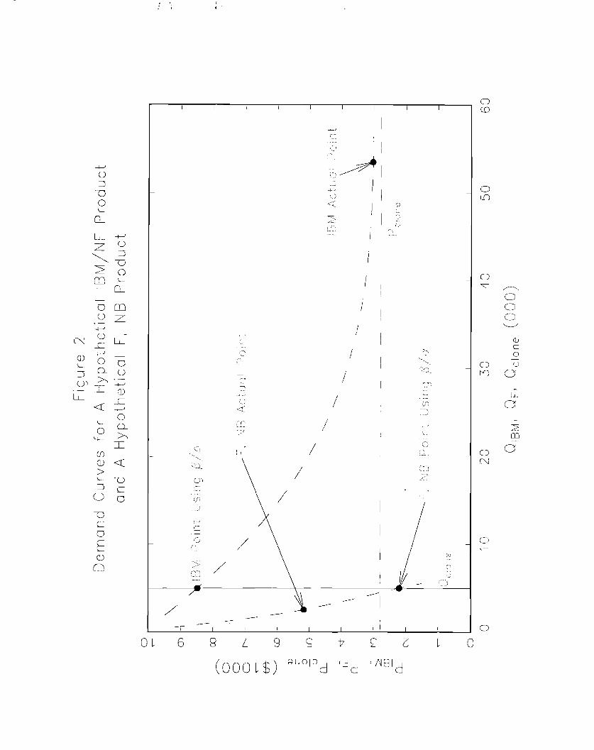
1

—

-—

I.,—:- 1,..I.

.

,.‘Al..,

II

.-.,..,..,

. ...

.,....,:.<...:.,

\.....,,....~.

-- ‘1

(vco

0

0

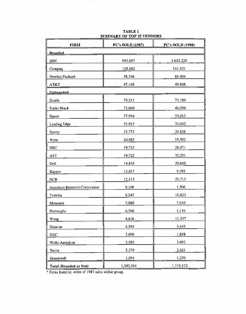
TABLE 1SUMMARYOF TOP 25 VENDORS

FIRM PC’SSOLD (1987) PC’SSOLD (19S8)

IBM 943,607 1,025,229

Compaq 128,682 141,621

HewIett-Packard 58,346 86,904

AT&T 47,168 49,608

Zenith 79,211 73,100

Radio Shack 75,600 46,030

Epson 37,916 55,015

Leading Edge 35,913 30,042

Sperry 25,773 30,838

Wyse 20,983 19,502

NEc 19,732 28,071

AST 19,722 32,201

Dell 14,836 20,600

Kaypro 13,837 9,393

NCR 12,115 25,713

American Research Corporation 9,108 1,506

Toshiba 8,243 10,823

Memorex 7,080 7,610

Burroughs 6,566 1,134

Wang 4,816 11,337

Datavue 4,594 3,445

DEC 2,609 1,898

Wells-American 2,580 3,492

Xerox 2,270 2,821

Honeywell 1,054 1,239

Total (Branded or Not) 1,582,361 1,719,172

* Firms listed in order of 1987 sales within group.

TABLE 2

SUMMARY STATISTICS BY YEAR

--l! 1987 1988

Mean Standard Mean Standard~Pviatinn Deviation

-

—-. .—----- —-. -—-----

13,077 32,856 12,549 28,721

Market Share II .00041 .0008 I .0003 I .0007

Price $3,226 $1,692 $3,205 $1,933

Frontier 0.10 0.30 0.15 0.35

Branded 0.30 0.45 0.30 0.45

RAM 611.47 403.73 688.26 504.21

MHZ II 3.751 9.491 4.67

Disk II 11.71 I 17.29 I 15.431 22.17

,’

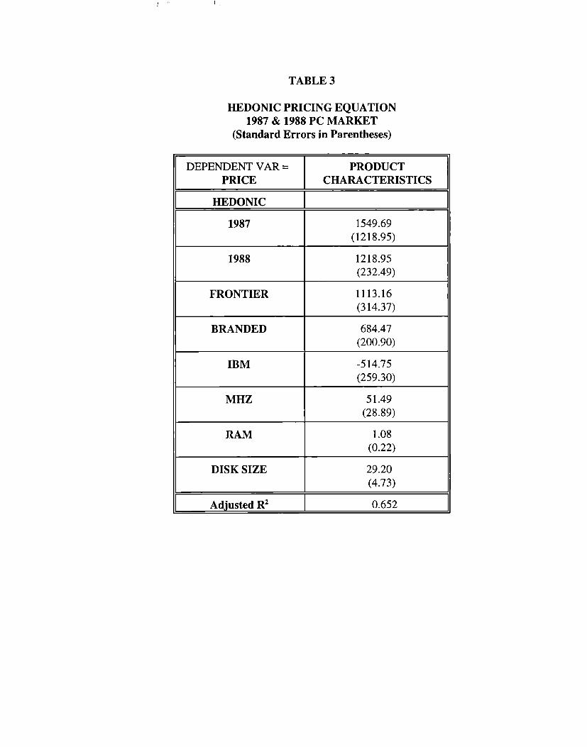
TABLE 3

HEDONIC PRICING EQUATION1987 & 1988 PC MARKET

(Standard Errors in Parentheses)

DEPENDENT VAR = PRODUCTPRICE CHARACTERISTICS

HEDONIC

1987 1549.69(1218.95)

1988 1218.95(232.49)

FRONTIER 1113.16(314.37)

BRANDED 684.47(200.90)

IBM -514.75(259.30)

MHZ 51.49(28.89)

RAM 1.08(0.22)

DISK SIZE 29.20(4.73)

I Adjusted R2 0.652

TABLE 4

SUMMARY STATISTICSBY CLUSTER BY YEAR

BRANDED

NON-BRANDED

YEA

#

QP

MHZ; RAM; Disk

#

QP

MHZ; RAM; Disk

= 1987

FRONTIER I NON-FRONTIER

587,058$7616

17.6; 1424; 59.8

717,740$5172

15.4; 1381;14.3

311,090,746

$31847.6; 506; 11.4

78386,826

$27867.7; 532; 6.5

BRANDED

NON-BRANDED

YEAR = 1988

#

QP

MHZ; RAM; Disk

#

QP

MHZ; RAM; Disk

FRONTIER

10203,466

$757719.6; 1531; 62.4

1028,188$5130

16.4: 1374:22.0

NON-FRONTIER

311,099,897

$29248.0; 493; 13.0

86387,631

$25748.0: 581:10.0

Legend

Number of Products

: Unit Sales -- Sum of all the products in the clusterP Mean Price

MHZ; RAM; Disk Mean [MHZ, RAM, Disk]

,. !.

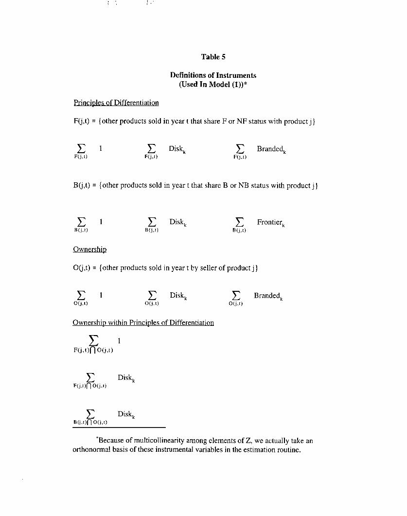
Table 5

Definitions of Instruments(Used In Model (l))*

Princit)les of Differentiation

F~,t) = (other products sold in year t that share F or NF status with product j }

xlF(j, t)

~ Disk,F(j, t)

~ Branded,F(j, t)

B~,t) ❑ {other products sold in year t that share B or NB status with product j }

xlB(j, t)

~ Disk,B(j, t)

~ Frontier,B(j, t)

Ownershiu

O(j,t) ❑ {other products sold in year t by seller of product j )

xlO(j, t)

~ Disk,O(j,f)

Ownership within Principles of Differentiation

X 1F(j, t)n O(j,t)

x Disk~F(j,t)n O(j, t)

x Disk~B(j,t)n O(j,[)

~ Branded,O(j,t)

*Because of multicollinearity among elements of Z, we actually take anorthonormal basis of these instrumental variables in the estimation routine.

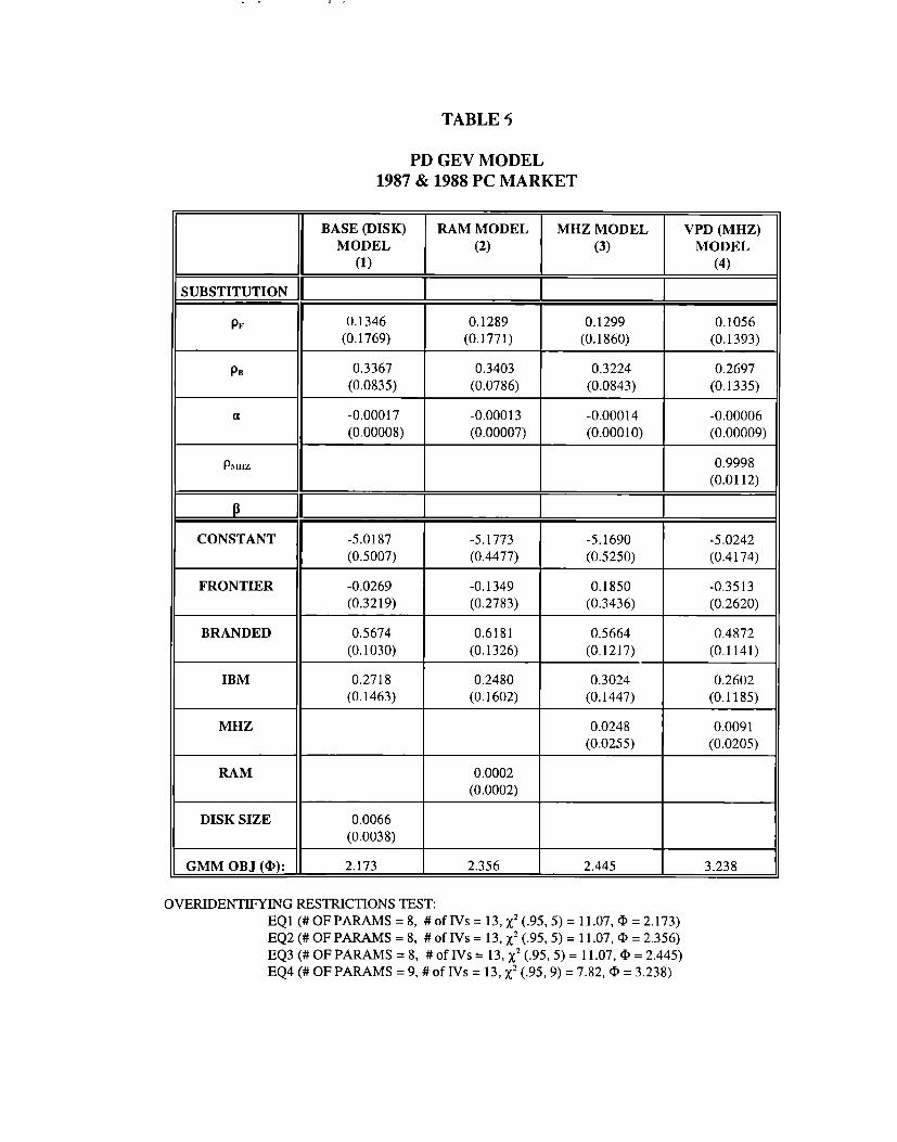
TABLE 5

PD GEV MODEL1987 & 1988 PC MARKET

BASE (DISK) RAM MODEL MHZ MODEL VPD (MHZ)MODEL (2) (3) MODEL

(1) (4)

1

PF 0.1346 0.1289 0.1299 0.1056(0.1769) (0.1771) (0.1860) (0.1393)

PB 0.3367 0.3403 0.3224 0.2697(0.0835) (0.0786) (0.0843) (0.1335)

a -0.00017 -0.00013 -0.00014 -0.00006(0.00008) (0.00007) (0.00010) (0.00009)

PnlHz 0.9998(0.0112)

~~

CONSTANT -5.0187 -5.1773 -5.1690 -5.0242(0.5007) (0,4477) (0.5250) (0.4174)

FRONTIER -0.0269 -0,1349 0.1850 -0.3513(0.3219) (0.2783) (0.3436) (0.2620)

BRANDED 0.5674 0.6181 0.5664 0,4872(0,1030) (0.1326) (0,1217) (0,1141)

IBM 0.2718 0.2480 0.3024 0.2602(0.1463) (O.1602) (0.1447) (0.1185)

MHZ 0.0248 0.0091(0.0255) (0.0205)

RAM 0.0002(0.0002)

DISK SIZE 0.0066(0.0038)

GMM OBJ (@): 2.173 2.356 2.445 3.238

OVERIDE~~G RESTRICTIONS TEST:EQ1 (#OF PARAMS = 8, #of lVs = 13, ~’ (.95, 5)= 11.07, @ = 2.173)EQ2 (# OF PARAMS = 8, #of IVs = 13, ~2 (.95, 5)= 11.07,0 = 2.356)EQ3 (# OF PARAMS = 8, #of IVs = 13, %’(.95,5)= 11.07,@= 2.445)EQ4 (# OF PARAMS = 9, # of IVs = 13, x’ (.95, 9) = 7.82, @ = 3.238)

TABLE 7

PD GEV VERSUS TWO-LEVEL NML MODELS1987 & 1988 PC MARKET

3H ‘i%i%‘giFSUBSTITUTION ~~

pF 0.1346 0.2309 0.4163(0.1769) (0.3029) (0.2830)

pB 0.3367 0.0437 0.9429(0.0835) (0.0147) (0.8890)

-0.00017 -0.00004 -0.00015(0.00012)

+ & ~

CONSTANT -5.0187 -4.4696 -5.4471(0.5007) (0.0621) (0.9444)

FRONTIER -0.0269 0.0124 -1.0365(0.3219) (0.0522) (0.7299)

BRANDED 0.5674 1.1131 0.4038(0.1030) (0.0077) (0.3496)

IBM 0.2718 -0.0169 0.4255(0.1463) (0.0188) (0.2889)

DISK SIZE 0.0066 0.0021 0.0076(0.0038) (0.0003) (0.0055)

GMM OBJ (0): -~ 0.223 2.492----- —---- ------ -- —.—--- —----- ——-—U VEKWEN 1lY YING WS”l’KIC1’lUNS “lES’l’:

EQ5 (#OF PARAMS = 8, # of IVs = 13, X2(.95,5)= 11.07, @ = 0.223)EQ6 (# OF PAR4MS =8, # of IVs = 13, X2(.95,5)= 11.07, 0=2.492)

TABLE 8

PD GEV MODELALTERNATIVE TREATMENTS OF THE INSTRUMENTS VECTOR

1987 & 1988 PC MARKET

qHmHSUBSTITUTION ~~~

=BB i, ::,

~~~~

CONSTANT -5.4692 -5.0187 -6.27 -4.7976

(0.4061) (0.5007) (15.99) (0.4054)

FRONTIER -0.4067 -0.0269 -0.0994 -0.6361

(0.2582) (0.3219) (2.625) (0.7549)

BRANDED 0.5190 0.5674 0.6982 0.3938(0.0911) (0.1030) (0.3348) (0.1261)

IBM 0.3627 0.2718 0.5884 0.2046(0.1296) (0.1463) (4.4384) (0,1135)

DISK SIZE 0.0029 0,0066 -0.0069 -0.0003(0.0019) (0.0038) (0.0308) (0.0047)

GMM OBJ (0): ~~ 0.526 0.238

VERIDENTIFYING RESTRICTIONS TEST:EQ7 (# OF PAR4MS = 8, #of IVs = 14,X2 (.95,6)= 12.59,@= 2.349)EQ8 (# OF PAR4MS = 8, #of ~S = 8, NO OVERIDENT RESTRICTIONS)EQ9 (# OF PAWMS = 8, #of IVS = 8, NO OVERIDENT RESTRICTIONS)

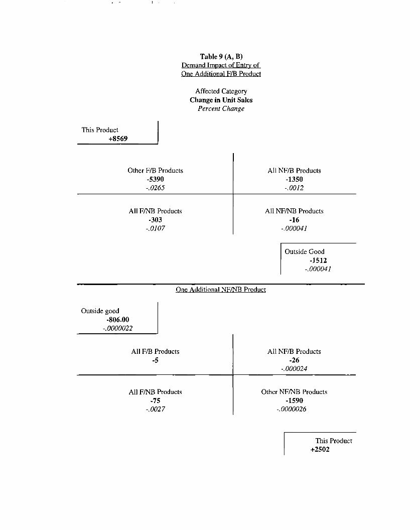
!. 1

Table 9 (A, B)Demand Imoact of Entw ofOne Additional F/B Product

Affected CategoryChange in Unit Sales

Percent Change

This Product+8569

Other F/B Products-5390-.0265

All NF/B Products-1350-,0012

All F~ Products-303

-.0107

All NF~ Products-16

-.000041

Outside Good

-1512

-.000041

One Additional NF/’NB Product

Outside good

-806.00-,0000022

All F/B Products-5

All NF/B Products

-26

-.000024

All F~ Products-75

-.0027

Other NF~B Products-1590

-.0000026

This Product

+2502

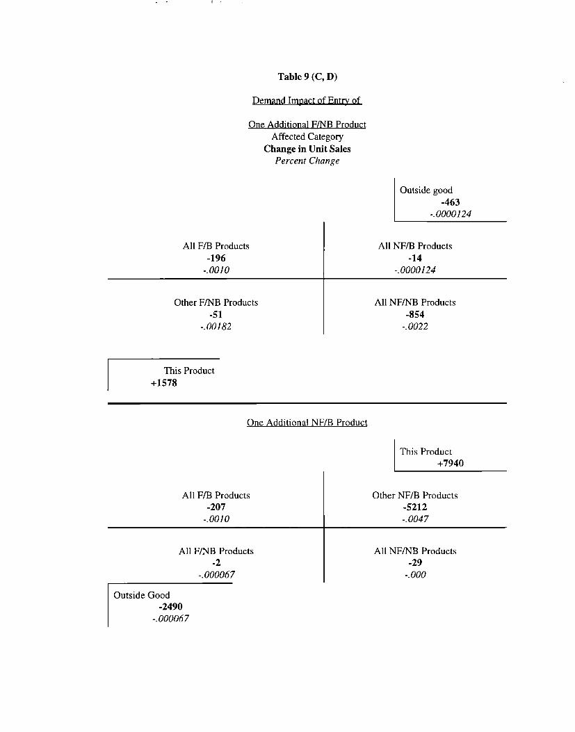
1

Table 9 (C, D)

Demand Imuact of EntU of

One Additional F/NB Product

Affected Category

Change in Unit SalesPercent Cltange

Outside good

-463

-.0000124

All F/B Products-196

-.0010

IOther F~B Products

-51-.00182

F

All NF/B Products

-14

-.0000124

All NF/NB Products-854

-.0022

All F/B Products-207

-.0010

One Additional NF/B Product

This Product

+7940

All F~B Products

-2

-.000067

Other NF/B Products

-5212

-.0047

All NF/NB Products

-29

-.000

Outside Good-2490

-.000067

Table 9 (E)

Market-S tealin~ Se~mentation

Qf,b

Product Introduced in

F, B

F, NB

NF, B

NF. NB

A Qpc

Qw

T1987 1988

-14.9 -6.5

(5.4) (4.3)

-9.5 -2.8

(14.9) (1.7)

-1.4 -1.5(.04) (.03)

&* Standard errors in parenthesis.