Market Informational Inefficiency, RiskAversion and Quantity Grid∗

Jean-Paul DECAMPS†and Stefano LOVO‡

January 9, 2003

Abstract

In this paper we show that long run market informational ineffi-ciency is perfectly compatible with standard rational sequential trademodels. Our inefficiency result is obtained taking into account twofeatures of actual financial markets: tradable quantities belong to aquantity grid and traders and market makers do not have the same de-gree of risk aversion. The implementation of our model for reasonablevalues of the parameters suggests that the long term deviations be-tween asset prices and fundamental value are important. We explainthe ambiguous role of the quantity grid in exacerbating or mitigat-ing market inefficiency. We show that stock splits can improve theinformation content of the order flow and consequently increase pricevolatility. (JEL G1, G14, D82, D83)Keywords: Informational efficiency, quantity grid, stock splits.

∗We would like to thank Bruno Biais, Thierry Foucault, Christian Gollier, Ulirch Hege,Jacques Olivier and Jean-Charles Rochet for insightful conversations and valuable advice.We would also like to thank the seminar participants at Turin University and the partic-ipants to the Sixth Toulouse Workshop in Finance for useful comments and suggestions.Of course all errors and omissions are ours.

†GREMAQ-IDEI Université de Toulouse 1, 21 Allee de Brienne, 31000 Toulouse,France, e-mail: decamps@cict.fr

‡HEC, Finance and Economics Department, 1 Rue de la Liberation, 78351, Jouy enJosas, France, e-mail: lovo@hec.fr.

1

1 Introduction

One of the central roles of financial markets is to provide information aboutasset’s fundamentals through the price system. After the recent collapse ofcompanies that were commonly considered, and priced, as worthy and safe,investors questioned the capacity of the market to perform this crucial task.For example, it is now clear that Enron’s fall was long time coming andthat pieces of information about the company’s problems were spread amongagents. Then, why have the price of Enron’s shares remained for so long farabove the company’s fundamental value?In financial economics, it is generally accepted that when it is possible

to observe the actions of a sufficiently large number of rational investors,deviations between transaction prices and long-term market fundamentaleventually vanish.1 This happens because each investor’s action discloses,at least partially, the investor’s private information on fundamental. Thisinformation is incorporated into the trading prices. Thus, by observing theseprices, it is ultimately possible to infer all the relevant private informationthat is dispersed among market participants. In other words, in the long run,the market is informational efficient. For this reason, some practitioners andfinancial economists attributed mispricing episodes to market exuberance orinvestors irrationality.In this paper we show that long term mispricing is perfectly compatible

with agent’s rationality. To this purpose, in a standard microstructure model,we jointly consider two features of financial markets: tradable quantitiesbelong to a quantity grid (in particular it is impossible to trade fractionsof a share); traders and market makers do not have the same degree ofrisk aversion. We show that when these two factors are taken into account,then market is not informational efficient in the long run. In other words,surprisingly, in the long term the private information regarding the assetfundamental value cannot be completely incorporated into trading prices.As in the model we consider, trading prices are equal to the expected valueof the risky asset given the history of trades, we can measure the long-term-mispricing with the distance between the trading prices in the long run andthe expected value of the asset for someone who has the combined knowledgeof all traders in the economy. We show that in general this distance cannot

1This is a textbook result in financial economics. See for example O’Hara (1995)or Biais, Glosten and Spatt (2001) for a recent review of the financial microstructureliterature.

2

vanishes, and that the resulting “long term pricing error" can be large. Thiscould provide a partial explanation to the episodes mentioned above.More precisely, the model we consider is a sequential trade model similar

to Glosten and Milgrom (1985) and Glosten (1989): in each period riskneutral market makers quote a price schedule for a risky asset. Given theprice schedule, informed risk averse traders choose the size of their trade.The difference with the existing literature is that we bring together on theone hand the existence of a grid for tradable quantities, on the other hand,discrepancy in risk aversion between dealers and traders.In order to have an intuition of our result, notice that a risk averse pri-

vately informed trader’s order includes two components: an informationalcomponent and an inventory component. The first component comes fromthe trader’s informational advantage given by his private information on theasset’s fundamental. The latter component follows from the trader’s riskaversion and is not related to the asset’s fundamental. Note that when thepast history of trades provides a sufficiently precise information about the as-set’s fundamental, then an additional partially informative private signal willaffect slightly a trader’s belief. Thus, as a trader can demand only discretequantities of the asset, a small change in his belief will in general not be suf-ficient to affect his demand and so, eventually all traders’ demands will onlyreflect their inventory components. From this point on, the flow of tradeswill no longer be informative, the social learning process stops and tradingprices will be bounded away from market fundamental. Long-run-mispricingwill increase with traders’ risk aversion and with the fundamental’s volatilitythat cannot be explained through private information. It will decrease withthe precision of traders’ private signals.In short, when the market is quite sure about the asset fundamental, the

equilibrium is unique and such that the flow of trade does not provide infor-mation because orders only reflects traders’ inventory concerns. Moreover,if the learning process stops when the market is quite sure about the asset’sfundamental but in a completely wrong direction, then prices will be trappedfar away from the asset fundamental value, and consequently the long termpricing error will be large.Other papers in the financial microstructure literature have considered

separately the discrepancy in risk aversion and discrete trading without ob-taining informational inefficiency. For example, in Glosten and Milgrom(1985) or Easley and O’Hara (1992) traders can only trade discrete quan-tities (buy 1 asset, sell 1 asset, no trade) but in these models both market

3

makers and informed traders are risk neutral, so trades are always informa-tive because of the absence of the inventory component. In Glosten (1989)and Biais, Martimort and Rochet (2000) risk neutral market makers facerisk averse informed traders, but these models assume that it is possible totrade a continuum of quantities of the asset so that even a tiny informationcomponent can affect the trader’s order, and for this reason the order flow isalways informative. Thus, our contribution is to show that the combinationof risk aversion and discrete trading generates informational inefficiency aslearning process stops at wrong price. Moreover, we show that mispricingcan be large even for realistic calibrations of the model.Our main result is in line with the theoretical literature on “herd behav-

ior” that proves that sequential interaction of rational investors can generaterational imitative behavior and this prevents agents from learning the mar-ket fundamental.2 However, most of the results in this literature are basedon the assumption that transaction prices are exogenously fixed and are notaffected by the information provided by past trades. Therefore, the herd-ing literature cannot be directly applied to stock markets, and it is clearlyunfit to study the issue of the informational content of prices. An informa-tional inefficiency result in presence of endogenous price is obtained by Lee(1998). He shows that information aggregation failure is due to the existenceof exogenous transaction costs. When the profit from trade is smaller thanthe transaction cost, investors stop trading and this prevents the completelearning of market fundamental. Décamps and Lovo (2002) and Cipriani andGuarino (2002) show that in a model where traders strategies are restricted(buy one lot, sell one lot, no trade) herd behavior and long run inefficiencycan occur because of differences in agents’ valuation for the asset.In this paper we show that informational inefficiency is not necessarily

linked to the presence of exogenous frictions in transaction prices due toinelastic prices (as in the rational herding literature), transaction cost (asin Lee (1998)) or exogenous difference in agents valuation for the object (asCipriani and Guarino (2002)).One might wonder whether our theoretical result can account for relevant

long run mispricing even when the lot size is one share. Indeed, with theadvent of on-line trading, traders can trade any integer size without much ofa problem. Can a one-share-discreteness actually induce significant long runmispricing? In order to answer this question, we implement our model for

2See Chamley (2001) for an extensive study on the causes of rational herding.

4

reasonable values of parameters. We measure the market inefficiency of anodd lots trading mechanism for a share with expected value 35$ and standarddeviation 7$. We find that, for reasonable level of traders’ risk aversion andprivate information, the minimum long-run pricing error is about 1.16 $ (i.e.3.31% of the expected value of the asset), the maximum pricing error can beabout 5,84 $ (i.e. 16.93% of the expected value of the asset) and the expectedpricing error is about 1.93$. (i.e. 5.52% of the expected value of the asset).We also prove that a change in the minimum trading unit (or lot size)3

has an ambiguous effect on informational inefficiency. On the one hand, anappropriate increase in the minimum trading unit can eliminate the long runmispricing. However, the choice of such an “informational-efficient lot size"is not robust to perturbations of the fundamentals of the economy. This sug-gests that it can be actually difficult to restore efficiency through the choiceof an appropriate grid of tradable quantities. On the other hand, decreasingthe lot size reduces, but does not eliminate, the long term inefficiency. Thelatter observation allows to relate our analysis to the literature on stock splits.Indeed, a stock split corresponds to a reduction of the minimum trading unitand therefore stock splits reduce market inefficiency. More precisely, a stocksplit can temporarily restore the informativeness of trades and consequentlyincrease price volatility. This could give reasons for the empirical findingsthat a stock split generates higher volatility in the stock’s return (Ohlsonand Penman’s (1985), Koski (1998)). Moreover, the same mechanism couldmotivate manager with favorable information about their company to splittheir share in order to allow market prices to further incorporate this posi-tive information. This could be an explanation of the empirical observationthat stock splits are associated with significant increases in the stock prices(Lamoureux and Poon (1987), Amihud et al. (1999)).In Section 2 the notations, the assumptions and the basic structure of

the model are presented. Section 3 shows the main result. In Section 4 weimplement the model and we discuss stock splits. In Section 5 we generalizethe inefficiency result to a broader class of economies. Section 4 concludes.The proofs are in the Appendix.

3The minimum trading unit corresponds to the tick of the quantity grid.

5

2 The model

We consider a sequential trade model in the style of Glosten and Milgrom(1985) and Glosten (1989): a risky asset is exchanged for money among mar-ket makers and traders. We denote with v = V+ ε the fundamental valueof one share of the asset. v is the sum of two components: a realized shockV on which agents are asymmetrically informed, and a noise ε that repre-sents the shocks on fundamental whose realization is unknown to everybodysuch as for example future shocks4. For expositional clarity we introducesome simplifying assumptions on the distribution of V and ε. The generalcase is discussed in Section 5. We assume that V and ε are independentlydistributed and that V is equal to V with probability π0 and to V < V withprobability 1− π0, moreover ε has zero mean and strictly positive standarddeviation σε. Remark that V is an unbiased estimator of v, but know-ing V is not sufficient to know the exact value of v. Each trader receivesa private partially informative signal s ∈ l, h. Signals are conditionallyi.i.d. across traders and independent from ε and from the compositions oftraders’ portfolios. We assume Pr(s =l|V = V ) = Pr(s =h|V =V ) = p with1/2 < p < 1. The parameter p represents the precision of the signal. Signall is more likely when V = V and it can be interpreted as a “Bearish” signal.Similarly, s = h can be interpreted as a “Bullish” signal. In other words,E[v|s = l] < E[v] < E[v|s = h]5.

Trading mechanism. Trading occurs sequentially and time is discrete.Each time interval is long enough to accommodate the trade of at most onetrader. At the beginning of each trading period a trader receives a privatesignal s and comes to the market with an endowment of shares known onlyto him. The trader submits a market order and market makers competeto fill the trader’s order without knowing the trader’s signal and portfoliocomposition. We assume that traders leave the market after they have hadthe opportunity to trade. We restrict the tradable quantities to belong to aquantity grid. We denote by δ the minimum trading unit. In other words, a

4This way of modelling the information structure is borrowed from Biais, Martimortand Rochet (2000). The noise ε takes into account that, as in reality, uncertainty is nevercompletely resolved.

5The results of the paper do not rely on the independence between V and ε, theirbinomial distribution nor on the fact that the precision of the signal is the same for allthe agents. See Section 5 for the treatment of the general case.

6

trader’s market order can be any integer multiple Q (positive or negative) ofa lot of δ shares of the asset. Note that our restriction to discrete quantitiesreflects the intrinsic nature of financial markets. If the exchange’s rules allowto trade any integer number of shares, then δ = 1. This is the case for oddlots trading mechanisms. By contrast, if only round lots can be traded, thenδ is greater than one and it represents the amount of shares in a round lot.6

Market participants. Market makers are risk neutral and traders are riskaverse.7 A trader’s expected utility obtained from a portfolio that containsan amount X of the risky assets and M of cash is E[u(M + Xv)], whereu0 > 0 and u00 < 0. For simplicity, we assume that all traders have thesame utility function8 but they can differ for the initial compositions of theirportfolios that are assumed to be independently and identically distributed.We denote x andm the initial amounts of risky asset and money respectivelyfor a given trader. Note that x is an integer number (positive or negative) astraders cannot hold fractions of shares of the asset, hence x ∈ Z andm ∈ R.9We will refer to x as the trader’s inventory. For a set Θ ⊂ Z × R, we useF (Θ) = Pr((x,m) ∈ Θ) to denote the probability that in a generic period t,the portfolio composition of a trader is in Θ. We assume that there exist abounded set bΘ ⊂ Z×R such that F ³bΘ´ = 1.Public and private belief. We denote Ht the history of trades up to time

t − 1. All the agents observe Ht but they do not know the identity of pasttraders. As private signals provide information on the realization of V butnot on the realization of ε, the learning process on the asset’s fundamentalonly regards V. The presence of ε guarantees that the uncertainty on vremains even when the realization of V is commonly known. We denote πt =Pr£V =V |Ht

¤the public belief at time t. If in period t a trader submits an

order of size Q, then public belief will evolve according to Bayes’ rule: πt+1 =Pr£V =V |Ht, Q

¤. We denote v(πt) = E[v|Ht] = E[V|Ht] the expectation

of v when the belief is πt. A trader refines public information with the oneprovided by his private signal. We denote πst = Pr

£V =V |Ht, s

¤, s ∈ h, l,

6Usually, a round lot consists of a lot of 100 shares or a multiple thereof.7Though the crucial assumption is that market makers and traders have different de-

grees of risk aversion, the assumption that market makers are risk neutral simplifies theanalysis.

8See Section 5 for the case of heterogenous traders.9Z denotes the set of integer numbers, positive and negative.

7

an informed traders’ belief at time t.

Agents’ behavior and equilibrium concept. When a trader comes to themarket, he expects a pricing schedule Pδ(.) : Z→ R , with the interpretationthat if he submits a market order Q ∈ Z positive (negative), then he will buyδQ shares (resp. sell δQ shares) and pay (resp. receive) Pδ(Q) per share.Thus, if at the time t trader has portfolio (x,m), received the signal s andexpects a price schedule Pδ(Q), then he will demand the quantity

Q∗(x,m,Pδ, πt, s) = argmaxQ∈Z

E [u (m+ (x+ δQ)v− Pδ(Q)δQ) |Ht, s] .

Apart from the discreteness in the tradable quantities, competition amongmarket makers is modeled as in Glosten (1989) or in Kyle (1985). Followingthese papers, as market makers are risk neutral and competitive, any trade ofδQ shares must lead to a zero conditional expected profit. Considering thatmarket makers are ignorant of the portfolio composition and information ofthe trader who is trading, a price schedule must satisfy

Pδ(Q) = E[v|Ht, Q∗ = Q]. (1)

That is the market clearing price is equal to the market makers’ expectationof v conditional on what they learn about v from the past and current trades.

3 Informational inefficiency

This section contains our main result showing that if: (i) traders are riskaverse and market makers are risk neutral, (ii) agents can trade only discretequantities; (iii) all the private information is not sufficient to completelyresolve uncertainty, i.e. σε > 0;10 then in general the market is not informa-tional efficient.In the long run, the market is strong-form informational efficient if all the

information dispersed among the traders in the economy is eventually incor-porated into market prices. Considering that in our model, traders’ privateinformation only regards V, E[ε] = 0 and market makers are risk neutral,

10Consequently, uncertainty cannot be completely resolved even in the long term. Weshow however in Section 4 that this assumption is not necessary to generate inefficiency.

8

we have informational efficiency if the trading prices eventually converge tothe realization of V.

Definition 1: The market is strong-form informational efficient in thelong run, if

limt→∞

E[|Pδ(Q)−V|] = 0.

Note that trading prices reflect the information content of past and cur-rent trades, and that the information content of a trader’s order is boundedby the information content of the trader’s private signal. As signals are notperfectly correlated with V, in order to achieve full efficiency, trades mustnever cease to be informative. We provide a formal definition of not infor-mative trade:

Definition 2: A trader with portfolio (x,m) who expects a price schedulePδ is said to place a not informative order if the order is not affected by thetrader’s private signal, i.e.

Q∗(x,m, Pδ, πt, h) = Q∗(x,m,Pδ, πt, l).

According to this definition, a trader’s order is not informative wheneven knowing the trader’s portfolio composition (x,m), the observation ofhis order does not allow to infer whether he received a bullish or a bearishsignal. In other words, if a trade of size Q is not informative, then Pr(Q∗ =Q|V = V ) = Pr(Q∗ = Q|V = V ).We will show that under some conditions on the distribution F , if in

period t the public belief πt is sufficiently close to 1 or to 0, the ordersof all traders in the economy are not informative. In this instance, thelearning process stops and public belief and prices will not change anymore.Namely, trading prices will remain at level Pδ(Q) = E[V|Ht] for all Q andall following periods. This is usually referred as an informational cascade inthe herding literature (see for instance Bikchandani, Hirshleifer and Welch(1992)). Considering that no single order can fully reveal V, eventuallybelief πt will be close either to 1 or to 0, and so an informational cascade willoccur before market makers have completely learned V. Thus, contrary tothe common wisdom, the trading prices cannot aggregate completely privateinformation and the market is not informational efficient in the sense of

9

Definition 1. This phenomenon can led to important long-run mispricingepisodes. When, for instance, πt is sufficiently close to 1 but the actualfundamental V is equal to V , the long term pricing error will be close tov(π)− V ' V − V .In order to understand why traders’ orders eventually cease to be infor-

mative, it is useful to distinguish two components in the trading motiva-tions of a risk averse agent: the inventory component and the informationcomponent. The inventory component reflects the agent’s preference for low-risk-portfolios. It increases with the agent’s degree of risk aversion, andthe unresolved uncertainty about the asset’s fundamental. The informationcomponent reflects the changes in traders’ belief that follows a bearish or abullish signal and can be measured by πht −πlt.

11 As signals are not perfectlyinformative about V, the information component will decrease as the publicbelief πt approaches 0 or 1.12 In other words, if the trader is quite sure aboutthe realization ofV, a partially informative private signal will affect his beliefjust slightly. Now, as a trader can demand only discrete quantities of theasset, a small change in his belief will in general not be sufficient to affect hisdemand13 and so we will have Q∗(x,m, Pδ, πt, h) = Q∗(x,m, Pδ, πt, l). Thatmeans that, when the public belief is sufficiently close to 0 or to 1, in generala trader’s demand only reflects his inventory component.The formal proof is slightly more complex. Indeed, it is always possible to

imagine risk averse traders whose demand is informative no matter how closeto 1, or to 0, is the public belief πt. Thus, in order to characterize inefficientmarkets, we precede as follows: firstly we identify the traders that submitinformative orders even when πt is arbitrarily close to 1 or to 0. Secondly,we show that the market is informational inefficient if the probability ofobserving such “informative traders" is zero.Suppose that the belief πt is almost equal to 1, or to 0, and take a trader

that before receiving the private signal, was indifferent between demandingan amount ofQ∗ lots orQ∗+1. The demand of this trader will be informative.Indeed, after receiving a tiny informative signal this trader will demand Q∗

if the signal is bearish, whereas he will demand Q∗+1 if the signal is bullish.The following lemma characterizes the set of such traders:

11Indeed, if signals are informative we have πlt < πt < πht .12That is to say, limπt→0(π

ht − πlt) = 0 and limπt→1(π

ht − πlt) = 0.

13Note that this would not be that case if traders could demand a continuum of theasset.

10

Lemma 1 Take πt = 1 or πt = 0. For any n ∈ Z, there exist x∗(n), withδn < x∗(n) < δ(n + 1), such that if a trader’s inventory is x∗(n), thentrading −n lots or −n − 1 lots is optimal. If ε is symmetrically distributedthen x∗(n) = δ(n+ 1/2).

In other words, when πt is almost equal to 0 or to 1, the only traders whoseorders are informative, are those whose inventories are sufficiently close tox∗(n) for some n ∈ Z.14Consequently, if the quantity grid δ and -or- the traders’ portfolio distrib-

ution F are such that inventories of all traders are bounded away from x∗(n)for all n ∈ Z, then, by a continuity argument, when the public belief willbe close enough to 0 or to 1, the demand of all traders in the economy willreflect only the inventory component and will provide no information on V.In this instance the flow of trade will be no more informative and long runinefficiency will occur. Now we turn to the formal statement of our result.

Proposition 1 If for all n ∈ Z the distribution of traders’ portfolio compo-sition F is such that there is a zero probability that a trader’s inventory isclose to x∗(n), then there exists π > 0 and π < 1 such that for πt < π orπt > π,(i) all traders’s orders at date t are not informative about V. As a con-

sequence πτ = πt for all τ > t.(ii) the equilibrium is unique and the price schedule satisfies Pδ(Q) =

v(πt) for all Q ∈ Z.Proposition 1 shows that, when the public belief πt is sufficiently large (or

small) then the equilibrium exists, it is unique and not informative. Preciselythe equilibrium price schedule must be Pδ(Q) = v(πt) for all tradable quan-tities Q ∈ Z. The result is fairly robust as it is obtained without specifyingthe traders’ utility function nor the precise distributions of ε.15

When the hypothesis of Proposition 1 are satisfied, the financial marketcannot be informational efficient as the learning process stops as soon as thepublic belief πt crosses one of the threshold π or π. We call the regions (0, π)

14Note that even when πt = 1 or πt = 0 the asset is still risky because of the ε component.Thus traders trade in order to hedge the risk of their portfolio.15In order to obtain our inefficiency result we do not study the equilibrium for all levels

of the public belief π. Therefore we do not need to restrict our analysis to the case ofCARA utility function and normal distribution of ε, that are the usual assumptions infinancial microstructure literature.

11

and (π, 1) information traps. Indeed if after a trading history the publicbelief πt belongs to one of these two regions, it will not move anymore. Inthis case, all quantities of the asset will be traded at v(πt) per share, andthe trading price will not change for all the subsequent periods τ > t. Thiscan potentially lead to highly inefficient markets. For example, suppose thatV = V and that πt ∈ (π, 1), then no matter the trading history observedafter t, prices will remain at level P (Q) = v(πt) much larger than V .The following two corollaries enlighten the role of the lot size in exacer-

bating and mitigating informational inefficiency. For example it turns outthat it could be optimal to increase quantity grid in order to restore the mar-ket informational efficiency. Precisely, Corollary 1 states that if the quantitygrid is the finest one, that is δ = 1, then long run informational inefficiencyoccurs almost surely for all discrete distribution F of the traders’ portfolios.Corollary 2 shows that when the noise ε is symmetrically distributed it ispossible to find a quantity grid δ that guarantees long run market efficiency.

Corollary 1 An odd lot trading mechanism is informational inefficient.

Corollary 2 If ε is symmetrically distributed, then in a round-lot mecha-nism, long run informational efficiency can be obtained only by choosing aminimum trading unit δ such thatX

n∈ZF

µx = δ

µn+

1

2

¶¶> 0. (2)

In order to have informational efficiency in a round lot mechanism, thesize of the round lot δ must be chosen so that the probability of observinginformative order is positive also when the public belief πt reaches extremelevels. Thus, a regulator that is mainly concerned with the problem of infor-mational efficiency could choose the minimum trading unit that maximizesthe probability of observing orders from traders whose inventory is x∗(n). ForLemma 1, when ε is symmetrically distributed, we have x∗(n) = δ(n+ 1/2)that implies that the optimal δ only depends on the distribution functionF and not on traders’ utility functions. However, it is worth stressing thata mean-preserving asymmetric perturbation of the distribution of ε wouldchange the value x∗(n) and this would restore informational inefficiency inthe economy. Roughly speaking, informational efficiency appears to be veryfragile.

12

4 Implementation

In order to understand whether the inefficiency result of the previous sectioncan actually account for relevant pricing errors, in this section we consider aspecification of our model and we measure the predicted long term pricingerror for reasonable value of the parameters.Definition 1 and equation (1) suggest that informational efficiency prop-

erties of the market can be measured by the distance between the realizationof V and the trading price in the long run. Hence, the long-term pricingerror (LTPE thereafter) can be defined as the random variable LTPE =limt→∞

|V− v(πt)|. For Proposition 1, as soon as the public belief π reaches oneof the two information traps, we have Pδ(Q) = v(π) for all Q. Therefore, inthe long run trading price will be either close to v(π) or to v(π). Thus, athreshold π close to 0 and a threshold π close to 1 correspond to a relativelyefficient market. Indeed, on the one hand the prices can reach a region that isrelatively close to the true value of V and, on the other hand, the probabilityof observing a trading history that lead the public belief into the “wrong"information trap is low.In this section we study how π, π and LTPE are affected by traders’

degree of risk aversion, the volatility of the fundamental and stock splits. Tothis purpose, we consider an odd lot trading mechanism (δ = 1), and we adoptthe standard assumptions of the microstructure literature for what regardstraders utility function and the distribution of ε. That is to say that tradershave negative exponential utility function (with risk aversion coefficient γ)and that ε is normally distributed. From Corollary 1, we already know thatsuch a market cannot be informational efficient. The following lemma allowsus to characterize the belief thresholds π and π and to measure the degreeof inefficiency for reasonable parameters value.

Lemma 2 Let u(W ) = −e−γW , let ε → N(0, σε) and let δ = 1, then π(resp. π) is the minimum π > 1/2 (resp. maximum π < 1/2) such that thefollowing two expressions are satisfied

e−γ(v(π)+γσ2ε/2) ≤ πhe−γV + (1− πh)e−γV , (3)

eγ(v(π)−γσ2ε/2) ≤ πleγV + (1− πl)eγV . (4)

If for a given level π, the inequalities (3) and (4) are satisfied, then aninformed traders chooses to trade exactly his inventory (Q∗ = −x) no matter

13

the signal he received,16 and so his order will only reflects his inventoryconcerns.Note first that if γ is sufficiently large, then inequalities (3) and (4) will

be met17. This happens because when traders are sufficiently risk averse theinformational content of their order vanishes as they only trade to reduce therisk of their portfolio.Similarly, when the information content of signals is low, i.e. πh is close

to πl, inequalities (3) and (4) will be satisfied even if σε is arbitrarily small.18

This implies that the presence of the additional noise ε is not a necessarycondition to obtain informational inefficiency. Thus, even if the aggregationof all private information could resolve uncertainty almost completely, whentraders’ information is not precise19, the existence of a minimum tradingsize will induce traders to neglect their information and this will impede theconvergence of prices to fundamental.Finally, remark that there exists σε sufficiently large such that no matter

the level of public belief or the information content of the private signal, thetwo inequalities are satisfied. This means that if the uncertainty coming fromthe noise ε is sufficiently large with respect to the information provided bythe component V, then even signals that are perfectly informative about Vwill not be reflected in traders’ orders. Indeed, the asset will be too risky tobe hold even by traders that are perfectly informed about one component ofthe asset fundamental value.To sum up, when i) the traders’ risk aversion is high; or ii) the precision of

private signals is low; or iii) the volatility in market fundamental is mostly dueto shocks on which there is no information, then even an infinite sequence oftrades will not allow the market to aggregate the relevant private informationdispersed among traders.Starting from Lemma 2, it is possible to compute numerically π and π for

different levels of the contribution of the private information component tothe fundamental’s volatility, and for different levels of traders’ risk aversion.For Proposition 1 in the long run trading price will be either close to v(π)or to v(π), furthermore, given the symmetry of the parameters, we have

16Remark that as x ∈ Z and δ = 1, it is possible to trade δQ = x.17Indeed, an increase in γ increases the convexity of the exponential. Moreover, a

sufficiently large increase in γ reduces the left hand sides of expressions (3) and (4).18This follows from the convexity of the exponential.19From Bayes rule, the difference between πh and πl increases with the precision of the

signal p.

14

π = 1 − π. Consequently, the minimum LTPE is close to |V − v(π)| =|V −v(π)| = (1−π)(V −V ) while the maximum LTPE is close to |V −v(π)| =|V − v(π)| = π(V − V ). Finally, it is possible to approximate the expectedlong term pricing error20 with E[LTPE] ' 2π(1− π)(V − V ).We consider thereafter an asset whose ex-ante expected fundamental value

is E[v] = 35$, and whose ex-ante standard deviation is σ =pσ2V + σ2ε = 7$

that is 20% of its ex-ante value, where σ2V =14(V − V )2. This corresponds

to the magnitude of the average share price and annual volatility in the NewYork Stock Exchange.Figure 1 depicts π and π when keeping constant E[v] = 35$ and σ = 7$

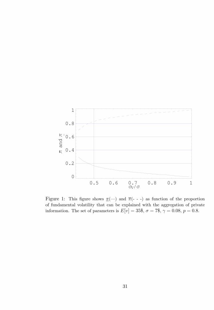
and varying σV/σ.21 The ratio σV/σ represents the proportion of the totalvolatility of asset’s fundamental that could be explained by aggregating allthe private information. The parameters set is (γ = 0.08, p = 0.8). WhenσV/σ increases, the information traps shrink and the market improves itsinformational efficiency. For example when σV/σ = 0.5, then π ' 0, 165 andπ ' 0, 835, whereas for σV/σ = 0.9 we have π ' 0, 021 and π ' 0, 979.Interestingly we also deduce from Figure 1 that, when the information inthe economy can explain less than 42% of the fundamental’s volatility, themarket mechanism fails completely to aggregate any private information.22

Table 1 reports approximations of the minimum LTPE , of the maximumLTPE and of the expected long run pricing error when varying σV/σ. Whenfor example 50% of the standard deviation of v could be explained with theprivate information, then the minimum LTPE is 1.16 $ and the maximumLTPE is 5.84 $. Saying it differently, in the long term the trading price iseither “wrong" by 1.16$ in one direction or by 5.84$ in the opposite direction,and the expected pricing error is about 2.25$. These pricing errors correspondto 3.31%, 16.93% and 5.52% of the expected fundamental value of the assetrespectively. The larger the ratio σV/σ, the smaller the expected long termerror.Figure 2 depicts π and π when changing the traders’ degree of risk aver-

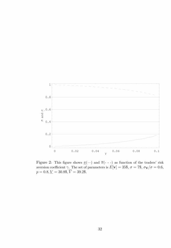
sion γ. The parameters set is (σV/σ = 0.6, p = 0.8). As the traders’ riskaversion increases, traders will exchange the asset mainly for inventory rea-son, the inventory component overwhelms the information component, andthe market informational inefficiency increases. For example when γ moves

20See the Appendix.21Note that in order to vary σV /σ keeping constant σ = 7$ and E[v] = 35$ it is necessary

to vary σε, V and V .22That is for all π ∈ (0, 1) the inequalities of Lemma 2 is satisfied.

15

from 0.02, to 0.08, π and π move from 0.015 and 0.985 respectively to 0,106and 0.894.Table 2 reports the approximations for the minimum, maximum LTPE

and the expected long run pricing error for different levels of traders’ riskaversion. For γ = 0, 06 the minimum and maximum LTPE are of 1.53% and22.45% of the ex-ante value of the asset respectively. The expected long runerror is about 1 $ that represents 2.87% of E[v]. An increase in traders riskaversion reduces the informational efficiency of the market.

4.1 Stock Splits

The market value of a firm’s equity is independent from the number of sharesoutstanding. Thus, a stock splits should not affect the distribution of stocksreturns. Nevertheless, Ohlson and Penman (1985) and Koski (1998) findthat stock return volatility increases after stock splits. Ohlson and Penmaninterpret this phenomenon as an increase in the presence of noise traders.Gottlieb and Kalay (1985) attributed this increase in volatility to the presenceof a price grid.23 However, in Koski (1998) the volatility increase does notappear to be due to rounding to discrete price level as suggested by Gottlieband Kalay. Our model provides an alternative explanation of the effects of astock split on price volatility and consequently return volatility.In order to see how a stock split increases price volatility, note first that a

stock split corresponds to a reduction of the minimum unit of trade. Indeed,before the stock split the fundamental value of one unit of trade is δv. Aftersplitting each share into n new shares, the fundamental value of each newshare will be v0 = v/n, and so the value of one lot of δ new shares is δv0 = δ

nv.

But this is perfectly equivalent to reducing the minimum unit of trade fromδ shares to δ/n shares without splitting the stock , in this case, the value ofthe new unit of trade would be δ

nv.

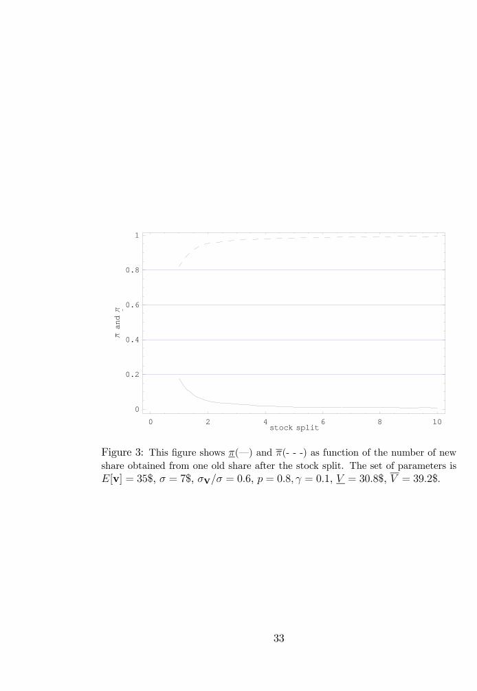
Second observe that a reduction of the unit of trade decreases π andincreases π. Figure 3 depicts π and π following a split of the stock. On thehorizontal axis there is the number of new share obtained from one old shareafter the stock split. The parameters set is (σV/σ = 0.6, p = 0.8, γ = 0.1).For the given levels of parameters, in the absence of a stock split we haveπ ' 0, 178 and π ' 0, 822 that correspond to an expected LTPE of 2.46$23Gottlieb and Kalay (1985) show that when continuous prices are rounded to discrete

price levels, the variance of return computed using the round prices exceeds the varianceof unrounded returns.

16

(see also Table 3). However, it is sufficient to split each share into twonew shares in order to obtain a dramatic reduction of the inefficiency as theexpected LTPE drops to 0.77$. Splitting each share into 10 new shares,we have π ' 0, 005 and π ' 0, 995 that is a huge informational efficiencyimprovement.How is this result related to price volatility? Note that as long as πt does

not lie into an information trap, trading prices can vary within a range ofabout v(π) − v(π). Thus, after a stock split this range increases allowing ahigher volatility for prices. Note also that a stock split can increase the pricevolatility by restoring the informativeness of trade in case of informationalcascade. For example, suppose that before the split, the public belief πt wasin an information trap. Then the asset is traded only for inventory reasons,trades do not transmit information on the asset fundamental, and tradingprices will be steady. In case of stock split, the information traps shrink,and for the same level of public belief πt, informativeness of trade can betemporarily restored. Thus the volatility of trading prices increases.24

5 Extensions

In order to simplify the analysis, in the previous sections we introduced somestrong assumptions on agent characteristics and on the distribution of therisky asset’s fundamentals. Namely we assumed homogeneity of traders’ util-ity functions, binomial distribution for V and s, and independence betweenV and ε. In this section we discuss the robustness of our result when thesethree assumptions are relaxed. We denote by v(Z,N) the fundamental valueof the asset that depends on two components: a realized shock Z on whichagents are asymmetrically informed, and a noiseN that represents the shockson fundamentals whose realization is unknown to everybody. Random vari-ables Z and N may lay in any measurable space, whereas v takes value inR+. We assume that the aggregation of all the private information that isdispersed among investors allows to know the realization of Z. Still, knowingZ will not be sufficient to completely resolve the uncertainty on the funda-

24Besides, the same mechanism can induce managers with favorable information abouttheir companies to split their share in order to allow a positive reaction of prices to theorder flow. This would provide a further explanation to the empirical observation thatstock splits lead to higher stock prices as shown by Lamoureux and Poon (1987) andAmihud et al. (1999).

17

mental value of the asset because of N. We denote V =E[v|Z] the expectedfundamental value of the asset after aggregating all the private information.And we denote ε = v−V the remaining error, where ε has zero mean andpositive standard deviation σε > 0. Thus, we can assume without loss ofgenerality that v = V + ε and that agents private information regards Vbut not ε.We assume that the random variable V takes value in a bounded set

Ω ∈ IR+. The random variables V and ε are not independently distributed.Still E[V] is an unbiased estimator of v: E[ε] = 0 and σε > 0. Eachtrader receives a partially informative private signal s that takes value in abounded set Σ. Without loss of generality, we assume that conditional onthe realization of V, private signals are independent. We assume that forall V ∈ Ω and s ∈ Σ, we have g(s|V ) = Pr(s = s|V = V ) > 0.25 Thatmeans that private signals are not perfectly informative as each realization ofthe signal is compatible with all realizations of V.26 Finally, we assume thatknowing a trader’s inventory does not change the expectation of V, that isto say that for all levels of inventory x and x0 we have

E[V|a trader’s inventory is x] = E[V|a trader’s inventory is x0].This last assumption guarantees that whenever a trader exchanges only forinventory reason his order will provide no additional information about V.27

Finally we assume that traders are risk averse but they can differ in theirutility functions and not only in the composition of their portfolio. Thefollowing proposition extends Corollary 1 to the general set up considered inthis section.

Proposition 2 An odd lot trading mechanism is informational inefficient.

Proposition 2 shows that market inefficiency does not rely on the simpli-fying assumptions we have introduced in the previous sections. Indeed, eventhe less risk averse trader who received the most precise signal, will even-tually trade only for inventory reason once the public beliefs are sufficiently25If s is continuously distributed g(.) shall be interpreted as the conditional density of

s.26This condition is equivalent the condition pql > 0 at page 1000 in Bikhchandani et al.

(1992).27Note that this is weaker than assuming independence between the distribution of a

trader’s private signal and his inventory. For instance, it is possible that traders with largeinventory in absolute value have more precise signals.

18

precise about market fundamentals. Thus, we can say that the informationalinefficiency arises when there is a general agreement on the asset’s funda-mental. In these cases, informed traders are prone to ignore their signalsand trade only for inventory reasons. Note also that our result is obtainedassuming that there is a zero measure of risk neutral traders. Décamps andLovo (2002) in a simplified model show that inefficiency can also occur whentraders are risk neutral provided that dealers are risk averse. This suggestthat what lead to inefficiency is not the absence of risk neutral traders butthe absence of traders whose utility functions are identical to those of marketmakers.

6 Conclusion

We studied the informational efficiency properties of a financial market whenone takes into account two factors: first, agents can trade only integer quan-tities of assets; second, traders and market makers do not have the samedegree of risk aversion. We show that an odd lot trading mechanism leadsto market inefficiency in the sense that in the long run, prices are boundedaway from the value of the asset given all the information dispersed in themarket. Indeed, when public belief are sufficiently precise, traders’ orderonly reflect their inventory concerns and thus provide no information aboutthe asset fundamental value. Implementing our model for reasonable valuesof the parameters leads to large long run pricing errors. Long run marketinefficiency increases with traders’ risk aversion, with the proportion of fun-damental’s volatility that cannot be explained with private information andit decreases with the precision of informed traders’ signals.We show that decreasing the unit of trade can reduce but does not elim-

inate market inefficiency. This provides an alternative explanation of theempirical observation that stock splits increase stock return volatility. Weshow that an appropriate increase of the minimum trading unit can restorecompletely long run informational efficiency. Still, the choice of an “effi-cient quantity grid" is not robust to small perturbation of the fundamentals’distribution.The fact that our results are obtained within a fairly general framework

and by introducing reasonable assumptions into standard microstructuremodels, suggests that the informational efficiency hypothesis is not com-

19

patible with the way economists are used to model the trading process infinancial markets.

7 Appendix

Proof of Lemma 1: Take πt = 1, in this case Pδ(Q) = V . Let U(x,Q) be atraders’ expected utility from trading Q at price V when his initial inventoryis x, i.e. U(x,Q) = E[u(m + xV + (x + δQ)ε]. Then from risk aversionand from the fact that traders wealth is bounded, we have that U(δn,−n) >U(δn,−(n+1)) and U(δ(n+1),−n) < U(δ(n+1),−(n+1)). Thus, from thecontinuity of U in x there exists x∗(n) ∈ (δn, δ(n+1)) such that if x = x∗(n),then the trader is indifferent between trading −n lots or −(n+ 1) lots.In order to see that when x = x∗(n) both these quantities are opti-

mal, note that if the trader could trade a continuum of quantities, then hewould trade exactly −x

δ. The trader is however constrained to trade integer

multiples of δ. Taking advantage from the concavity in Q of U(x,Q), theconstrained optimal tradable quantities are the closest to −x

δthat is −δn

and −δ(n+ 1). Finally if ε is symmetrically distributed, then ε and −ε areidentically distributed and so U(δ(n + 1/2),−n) = U(δ(n+ 1/2),−(n+ 1))that means x∗(n) = δ(n+1/2). The proof for the case πt = 0 is symmetric.

Proof of Proposition 1: Note first that as quotes must satisfy equation(1) and the informativeness of an order is bounded by the precision of atraders’ order, we have that in equilibrium, at any date t, v(πlt) ≤ Pδ(Q) ≤v(πht ) for all Q ∈ Z. Thus, for any price schedule Pδ(Q) satisfying thisproperty and for a trader with portfolio (x,m) we have:

E£u¡m+ (x+ δQ)v− δQv(πht )

¢ |s¤ ≤ E [u (m+ (x+ δQ)v− δQPδ(Q)) |s] ≤≤ E

£u¡m+ (x+ δQ)v− δQv(πlt)

¢ |s¤(5)

for Q positive, and

E£u¡m+ (x+ δQ)v− δQv(πlt)

¢ |s¤ ≤ E [u (m+ (x+ δQ)v− δQPδ(Q)) |s] ≤≤ E

£u¡m+ (x+ δQ)v− δQv(πht )

¢ |s¤(6)

20

for Q negative.Note that πst is continuous in πt and that u is a continuous function.

Moreover, when πt is close to 1 or to 0, an informative signal affects slightlythe informed trader belief, indeed πlt < π < πht and limπt→1(π

ht − πlt) =

limπt→0(πht − πlt) = 0. Thus, we have that:

limπt→1

E£u¡m+ (x+ δQ)v− δQv(πht )

¢ |s¤ = limπt→1

E£u¡m+ (x+ δQ)v− δQv(πlt)

¢= E

£u¡m+ xV + (x+ δQ)ε

¢¤.(7)

From Lemma 1 we know that if x 6= x∗(n) for all n ∈ Z, then there exist aunique bQ, such that for all Q 6= bQ, we have

Ehu³m+ xV + (x+ δ bQ)ε)´i > E

£u¡m+ xV + (x+ δQ)ε

¢¤.

Thus, from expression (7), it must be that for πt sufficiently close to 1 andfor all Q 6= bQEhu³m+ (x+ δ bQ)v− δ bQv(πht )´ |si > E

£u¡m+ (x+ δQ)v− δQv(πlt)

¢ |s¤ ,(8)

Ehu³m+ (x+ δ bQ)v− δ bQv(πlt)´ |si > E

£u¡m+ (x+ δQ)v− δQv(πht )

¢ |s¤ .(9)

Now take an informed trader whose inventory x is bounded away from x∗(n)for all n ∈ Z, and suppose he expects a price schedule Pδ(Q). His maximiza-tion problem will be:

argmaxQ∈Z

E [u (m+ (x+ δQ)v− δQPδ(Q)) |s] .

Then expressions (5), (6), (8) and (9) imply

Ehu³m+ (x+ δ bQ)v− δ bQPδ( bQ)´ |si > E [u (m+ (x+ δQ)v− δQPδ(Q)) |s]

for all Q 6= bQ. That is if πt is sufficiently close to 1, this trader will tradea quantity bQ no matter he received a bearish or a bullish signal. Thereforehis action will provide no information on V. To conclude the proof it is

21

sufficient to observe that because of the hypothesis on F , for all n ∈ Z thereis no trader whose inventory is not bounded away from x∗(n). Thus, traders’demand is not informative, and so, from equation (1), the price schedule mustbe Pδ(Q) = E[v|Ht] for all Q ∈ Z. In order words, when πt is sufficientlyclose to 1, there exist no equilibrium where the traders orders are informative.In order to prove that a not informative equilibrium exist, it is sufficient toobserve that for πt close to 1, Q∗(x,m, v(πt), πt, s) = bQ for all s. An identicalargument applies for πt sufficiently close to 0.

Proof of Corollary 1: Simply remark that from Lemma 1, when δ = 1we have x∗(n) ∈ (n, n+1). That means that when πt reaches extreme levels,the only traders whose orders are informative are traders that hold fractionsof the asset.28 However, all traders in the economy hold only integer amountsof the asset, x ∈ Z, and thus, from Proposition 1, eventually trade will stopproviding information on V.

Proof of Corollary 2: From Lemma 1 and Proposition 1 we know thatthe only traders whose orders are informative even when πt is arbitrarilyclose to 0 or to 1 are those whose inventory is equal to x∗(n) for some n ∈ Z.Moreover, if ε is symmetrically distributed we know that x∗(n) = δ

¡n+ 1

2

¢.

Therefore δ should be chosen such that there exist a positive probability ofobserving these traders, thus the inequality (2).

Proof of Lemma 2: From Proposition 1 we know that when all traders’orders are not informative, in equilibrium P (Q) = v(πt) for all Q. FromCorollary 1 we deduce that when πt is sufficiently close to 1 or to 0 andP (Q) = v(πt), then a trader with inventory x ∈ Z will trade exactly −x nomatter he received a bullish or a bearish signal. As the expression E[u(m+(x + q)v − v(πt)q)|s] is a strictly concave function in the traded quantityq ∈ R, then it will have a unique maximum. Thus in order to find π (resp.π), it is sufficient to find the minimum π > 1/2 (resp. maximum π < 1/2)such that the trader prefers to trade −x rather than −x − 1 or −x + 1 forboth s = h and s = l. That is to say

u(m+v(π)x) > maxE[u (m+ v + (x− 1)v(π)) |s], E[u (m− v + (x+ 1)v(π)) |s](10)

28Moreover, as the traders wealth is bounded, we know that x∗(n) is bounded awayfrom n or n+ 1.

22

for s = h and s = l. Considering that u(W ) = −e−γw and that ε → N(0, σε),we have that expression (10) is satisfied only if both inequalities in Lemma2 are met.

Approximation of the long term pricing error: Proposition 1 showsthat, at the equilibrium, the long term price eP ≡ limt→∞E[v|Ht] will beeither close to v(π) or to v(π). Assuming the initial public belief is 1

2, the ex

ante expectation of the long term pricing error can be approximated by

E[LTPE] ' 1

2(V − v(π))Pr(P ≥ v(π)|V = V )+

+1

2(V − v(π))Pr(P ≤ v(π)|V = V )+

+1

2

³(v(π)− V )Pr(P ≥ v(π)|V = V ) + (v(π)− V )Pr(P ≤ v(π)|V = V )

´.

Indeed the probability that the long term price being close to v(π) is equalto the probability of the public belief reaches the level π. Moreover, fromthe symmetry of the model we deduce that given that (P ≥ v(π)|V = V ) =Pr(P ≤ v(π)|V = V ). Based on the first passage time approach developedin Diamond and Verrechia (1987) we obtain a proxy for the long term pricingerror:

Claim: Assuming the initial public belief is 12, a proxy for the expectation

of the long term pricing error is given by

2π π (V − V ).

We prove this Claim as follows: Let consider the likelihood ratio Lt =πt1−πt . We have Lt = Πi=t

i=1r(Qi, πi) where r(Qi, πi) =Pr(Qi |V=V ,Hi)Pr(Qi |V=V ,Hi)

. Theratio r(Qi, πi) is interpreted as the informative content of trader i’s order ofsize Qi. As we do not know the equilibrium strategies when πt ∈ (π, π), weapproximate the information content of a trade assuming that as long as πt ∈(π, π)market makers can perfectly infer the traders’ signals from their orders.Thus, as long as πt ∈ (π, π), the ratio r(Qt, πt) takes the value

p1−p when the

trader’s order Qt reveals a bullish signal and the value1−ppwhen the order Qt

reveals a bearish signal. Consequently, under this approximation, r(Qt, πt)does not depend on πt. Now, consider N = inft s.t. Lt /∈ ( π

1−π ,π1−π ),

23

the random variable representing the number of periods before bound π1−π

or bound π1−π is passed. The probability that the public belief πt reaches

the threshold π given that the fundamental value of the asset is V is equalto Pr(LN ≥ π

1−π | V = V ). Using the same techniques29 than Diamond

and Verrechia (1987), we obtain Pr(LN ≥ π1−π |V = V ) = (1−2π)(1−π)

π−π , and

Pr(LN ≤ π1−π |V = V ) = (2π−1)π

π−π from which we deduce our result.

Proof of Proposition 2: The proof is similar to the proof of Proposition1. First we show that the price schedule has an upper and a lower bound thatconverge to E[V] as public information becomes sufficiently precise. Thenwe show that, whenever trading prices are sufficiently close to E[V] andpublic information is sufficiently precise, all risk averse traders will optimallychoose to trade Q∗ = −x no matter the signal they received. Thus, theinformational content of the order flow vanishes and prices will not convergeto fundamental.

We say that the public ex-ante belief is sufficiently precise at time t ifV ar(V|Ht) is positive but sufficiently close to 0. Remark that precisenessof ex-ante public belief has nothing to do with the fact that agents’ beliefare actually correct. Indeed, very precise public belief can turn out to becompletely wrong.Now, for any finite history Ht it is always possible to find two signals in

Σ that ,with an abuse of notation, we will denote l and h, such that

E[V|Ht, s = l] ≤ E[V|Ht, s = s] ≤ E[V|Ht, s = h]

for all s ∈ Σ. Note that, from standard property of the conditional variancewe have V ar (V|Ht) = E [V ar (V|Ht, s)] + V ar (E [V|Ht, s]). Thus, ifV ar (V|Ht) lies in a small neighborhood of 0 then it is also the case forV ar (V|Ht, s). Moreover, as g(s|V ) > 0 for all V ∈ Ω and s ∈ Σ, wehave that E[V|Ht, s = h] − E[V|Ht, s = l] is close to 0 when V ar(V|Ht)is sufficiently close to 0. In other words, if the public belief is sufficientlyprecise, then private signals affect private beliefs just slightly.

Now, consider that market makers cannot infer from a trader’s order morethan what the trader know, and that a trader’s inventory does not provide29Precisely we use theorem 9.34 page 549 of Schervish (1995). In a related vein we can

deduce from the Wald’s lemma page 552 of Schervish (1995) that our proxy underestimatesthe average long term pricing error.

24

information about the expectation of V. Thus, from equation (1) we havethat at time t the price schedule satisfies

E[V|Ht, s = l] ≤ Pδ(Q) ≤ E[V|Ht, s = h], ∀Q ∈ Z.

Let ui be a trader i’s utility function that is continuous strictly increasing andconcave. Let denote vlt = E[V|Ht, s = l], and vht = E[V|Ht, s = h]. Thenequations (5) and (6) still hold after substituting ui, vht , v

lt to u, v(π

ht ), v(π

lt)

respectively. Moreover, because of risk aversion E [ui (m+ xV + (x+ δQ)ε)]is maximized for Q∗ = −x. If V ar(V |Ht) is sufficiently small, then equations(8) and (9) will still hold after substituting ui, vht , v

lt and −x to u, v(πht ),

v(πlt) and bQ respectively. Thus for V ar(V |Ht) sufficiently close to 0:

argmaxQ∈Z

E [ui (m+ (x+ δQ)v− δQPδ(Q)) |s] = −x ∀s ∈ Σ.

That means that when public belief are sufficiently precise, traders’ orderonly reflect their inventory concerns and provides no information about V.

8 References

Amihud Y., H. Mendelson and J. Uno, 1999, “Number of Shareholders andStock Prices: Evidence from Japan”, Journal of Finance, 54, pp. 1169-1184.

Biais, B., D. Martimort and J.C. Rochet, 2000, “Competing Mechanisms ina Common Value Environment”, Econometrica, 68, 4, 799-837.

Biais B., L. Glosten, and C. Spatt, 2002. “The Microstructure of Stock Mar-kets”. CEPR Discussion Paper no. 3288. London, Centre for EconomicPolicy Research. http://www.cepr.org/pubs/dps/DP3288.asp.

Bikhchandani S., D. Hirshleifer, I. Welch, 1992, “A Theory of Fads, Fashion,Custom and Cultural Change as Informational Cascades”, Journal of Polit-ical Economy, 100, pp. 992-1026.

Chamley C., 2001, “Rational Herds”, http://econ.bu.edu/chamley/chamley.html,University of Boston.

25

Cipriani M. , A. Guarino, 2002, “Herd Behavior and Contagion in FinancialMarkets”, mimeo, New York University.

Décamps J.P., S. Lovo, 2002, “Risk Aversion and Herd Behavior in FinancialMarkets”, HEC CR 758/2002.

Diamond D.W., R.E. Verrechia, 1987, “Constraints on Short-selling and As-set Price Adjustments to Private Information ”, Journal of Financial Eco-nomics 18, pp. 277-311

Easley D., M. O’Hara, 1992, “Time and the Process of Security Price Ad-justment ”, Journal of Finance, 57, pp. 577-605.

Glosten L., 1989, “Insider Trading, Liquidity and the Role of the MonopolistSpecialist”, Journal of Business, 62, pp. 211-235.

Glosten L., P. Milgrom, 1985, “Bid, Ask and Transaction Prices in a Spe-cialist Market with Heterogeneously Informed Traders”, Journal of FinancialEconomics, 14, pp. 71-100.

Gottlieb G and A. Kalay, 1985, “Implication of the Discreteness of ObservedStock Prices”, Journal of Finance, 40, pp. 135-153.

Koski J., 1998, “Measurement Effects and the Variance of Returns after StockSplits and Stock Dividends", Review of Financial Studies, 11, pp. 143-162.

Lamoureux C.G., P. Poon, 1987, “The Market Reaction to Stock Splits”,Journal of Finance, 42, pp. 1347-1370.

Lee I. H., 1998, “Market Crashes and Informational Avalanches”, Review ofEconomic Studies, 65, 741-759.

O’Hara M. , 1995, Market Microstructure Theory, Blackwell Publishers.

Ohlson J.A., S. Penman, 1985, “Volatility Increases Subsequent to StockSplits: An Empirical Aberration”, Journal of Financial Economics, 14, pp.251-266.

26

Schervish M.J, 1995, Theory of Statistics, Springer-Verlag New York, Inc.

27

Table 1: Long term pricing error for different σV/σ

σV/σ minimum LTPE maximum LTPE E[LTPE] Vvalue in $ % of E[v] value in $ % of E[v] value in $ % of E[v]

0.42 1.75 4.99% 4.13 11.61% 2.45 7.01% 330.5 1.16 3.31% 5.84 16.93% 1.93 5.52% 310.6 0.89 2.56% 7.51 21.44% 1.60 4.57% 300.7 0.69 1.97% 9.11 26.03% 1.28 3.67% 300.8 0.47 1.39% 10.71 30.61% 0.93 2.66% 290.9 0.26 0.74% 12.34 35.26% 0.51 1.45% 280.99 0.01 0.04% 13.85 29.56% 0.03 0.07% 28

Comparison of the long term pricing errors for different levels of σV/σ. Theparameter set is E[v] = 35$, σ = 7$, γ = 0.08, p = 0.8. The minimum LTPEis defined as π(V − V ), the maximum LTPE is defined as π(V − V ) and theexpected LTPE is defined as 2ππ(V − V ). All these measures are given both inabsolute value and in percentage of the ex-ante expected value of the asset E[v].

28

Table 2: Long term pricing error for different γ

γ minimum LTPE maximum LTPE E[LTPE]value in $ % of E[v] value in $ % of E[v] value in $ % of E[v]

0.01 0.06 0.16% 8.34 23.84% 0.11 0.32%0.02 0.12 0.35% 8.28 23.65% 0.24 0.69%0.04 0.29 0.84% 8.11 23.14% 0.57 1.62%0.06 0.53 1.53% 7.86 22.45% 1.00 2.87%0.08 0.89 2.56% 7.51 21.44% 1.60 4.57%0.1 1.50 4.28% 6.90 19.72% 2.46 7.03%0.11 2.05 5.84% 6.35 18.15% 3.10 8.85%

Comparison of the long term pricing errors for different levels of traders’ riskaversion γ. The parameter set is E[v] = 35$, σ = 7$, σV/σ = 0.6, p = 0.8, V =30.8$, V = 39.2$. The minimum LTPE is defined as π(V − V ), the maximumLTPE is defined as π(V −V ) and the expected LTPE is defined as 2ππ(V −V ).All these measures are given both in absolute value and in percentage of the ex-anteexpected value of the asset E[v].

29

Table 3: Long term pricing after a stock split

new shares minimum LTPE maximum LTPE E[LTPE]value in $ % of E[v] value in $ % of E[v] value in $ % of E[v

1 1.50 4.28% 6.90 19.72% 2.46 7.03%2 0.40 1.15% 8.00 22.85% 0.77 2.20%4 0.16 0.46% 8.24 23.54% 0.32 0.90%6 0.10 0.29% 8.30 23.71% 0.20 0.56%8 0.07 0.20% 8.33 23.79% 0.14 0.41%10 0.05 0.16% 8.34 23.84% 0.11 0.32%

Comparison of the long term pricing errors after splitting the stock in to 2to 10 new shares. The parameter set is E[v] = 35$, σ = 7$, σV/σ = 0.6,p = 0.8, γ = 0.1, V = 30.8$, V = 39.2$. The minimum LTPE is defined asπ(V −V ), the maximum LTPE is defined as π(V −V ) and the expected LTPEis defined as 2ππ(V − V ). All these measures are given both in absolute valueand in percentage of the ex-ante expected value of the asset E[v].

30

0.5 0.6 0.7 0.8 0.9 1σVêσ0

0.2

0.4

0.6

0.8

1

πdna

π −

Figure 1: This figure shows π(–) and π(- - -) as function of the proportionof fundamental volatility that can be explained with the aggregation of privateinformation. The set of parameters is E[v] = 35$, σ = 7$, γ = 0.08, p = 0.8.

31

0 0.02 0.04 0.06 0.08 0.1γ

0

0.2

0.4

0.6

0.8

1

πdna

π −

Figure 2: This figure shows π(–) and π(- - -) as function of the traders’ riskaversion coefficient γ. The set of parameters is E[v] = 35$, σ = 7$, σV/σ = 0.6,p = 0.8, V = 30.8$, V = 39.2$.

32

0 2 4 6 8 10stock split

0

0.2

0.4

0.6

0.8

1

πdna

π −

Figure 3: This figure shows π(–) and π(- - -) as function of the number of newshare obtained from one old share after the stock split. The set of parameters isE[v] = 35$, σ = 7$, σV/σ = 0.6, p = 0.8, γ = 0.1, V = 30.8$, V = 39.2$.

33