Markdown for Class Reports

Ozancan Özdemir

What is R Markdown?

R Markdown is a low-overhead way of writing reports which includes R code and the code’s automatically-generated output. It also lets you include nicely-typeset math, hyperlinks, images, and some basic formatting. The goal of this document is to explain, with examples, how to use its most essential features. It is not a comprehensive reference. (See rather http://rmarkdown.rstudio.com)

Mark Up, Markdown

You are probably used to word processing programs, like Microsoft Word, which employ the “what you see is what you get” (WYSIWYG) principle: you want some words to be printed in italics, and, lo, they’re in italics right there on the screen. You want some to be in a bigger, different font and you just select the font, and so on. This works well enough for n00bs but is not a viable basis for a system of text formatting, because it depends on a particular program (a) knowing what you mean and (b) implementing it well. For several decades, really serious systems for writing have been based on a very different principle, that of marking up text. The essential idea in a mark-up language is that it consists of ordinary text, plus signs which indicate how to change the formatting or meaning of the text. Some mark-up languages, like HTML (Hyper-Text Markup Language) use very obtrusive markup; others, like the language called Markdown, are more subtle. For instance, the last few sentences in Markdown look like this:

For several decades, really serious systems for writing have been based on a very different principle, that of _marking up_ text. The essential idea in a **mark-up language** is that it consists of ordinary text, _plus_ signs which indicate how to change the formatting or meaning of the text. Some mark-up languages, like HTML (Hyper-Text Markup Language) use very obtrusive markup; others, like the language called **Markdown**, are more subtle.

Every mark-up language needs to be rendered somehow into a format which actually includes the fancy formatting, images, mathematics, computer code, etc., etc., specified by the mark-up. For HTML, the rendering program is called a “web browswer”. Most computers which know how to work with Markdown at all know how to render it as HTML (which you can then view in a browser), PDF (which you can then view in Acrobat or the like), or Word (which you can then view in the abomination of Redmond).

The advantages of mark-up languages are many: they tend to be more portable across machines, less beholden to particular software companies, and more stable over time than WYSIWYG word processing programs. R Markdown is, in particular, both “free as in beer”

(you will never pay a dollar for software to use it) and “free as in speech” (the specification is completely open to all to inspect). Even if you are completely OK with making obeisance to the Abomination of Redmond every time you want to read your own words, the sheer stability of mark-up languages makes them superior for scientific documents.

Markdown is a low-overhead mark-up language invented by John Gruber. There are now many programs for translating documents written in Markdown into documents in HTML, PDF or even Word format (among others). R Markdown is an extension of Markdown to incorporate running code, in R, and including its output in the document. This document look in turn at three aspects of R Markdown: how to include basic formatting; how to include R code and its output; and how to include mathematics.

Openning R Markdown File

In order to create your .rmd file, click on select file, new file and r markdown respectively. Then, please enter Title, Author, and Output Format (this can be changed later). Then click on OK. You will get an example that you can alter or delete

Document Orientation

This document will cover 4 pieces of an R Markdown document.

Rendering and Editing

To write R Markdown, firstly, you will need a text editor, a program which lets you read and write plain text files. You will also need R with the lastest version, and the package rmarkdown (and all the packages it depends on).

• Most computers come with a text editor (TextEdit on the Mac, Notepad on Windows machines, etc.).

• You could use Word (or some other WYSIWYG word processor), taking care to always save your document in plain text format. I do not recommend this.

• R Studio comes with a built-in text editor, which knows about, and has lots of tools for, working with R Markdown documents.

If this is your first time using a text editor for something serious, I suggest you to use R Studio.

Rendering in R Studio

Assuming you have the document you’re working on open in the text editor, click the button that says “knit”. #### Kniting When you are ready, you can “knit” the document to some format. HTML is available right away, but you need to install a LaTeX package in order to knit to PDF or Word. Other options are available (e.g., kindle) if you

download other packages.

Basic Formatting in R Markdown

For the most part, text is just text. One advantage of R Markdown is that the vast majority of your document will be stuff you just type as you ordinarily would.

Paragraph Breaks and Forced Line Breaks

To insert a break between paragraphs, include a single completely blank line.

To force a line break, put two blank spaces at the end of a line.

To insert a break between paragraphs, include a single completely blank line. To force a line break, put _two_ blank spaces at the end of a line.

Headers

The character # at the beginning of a line means that the rest of the line is interpreted as a section header. The number of #s at the beginning of the line indicates whether it is treated as a section, sub-section, sub-sub-section, etc. of the document. For instance, Basic

Formatting in R Markdown above is preceded by a single #, but Headers at the start of this paragraph was preceded by ###. Do not interrupt these headers by line-breaks.

Italics, Boldface

Text to be italicized goes inside a single set of underscores or asterisks. Text to be boldfaced goes inside a double set of underscores or asterisks.

Text to be _italicized_ goes inside _a single set of underscores_ or *asterisks*. Text to be **boldfaced** goes inside a __double set of underscores__ or **asterisks**.

Quotations

Set-off quoted paragraphs are indicated by an initial >:

In fact, all epistemological value of the theory of probability is based on this: that large-scale random phenomena in their collective action create strict, nonrandom regularity. [Gnedenko and Kolmogorov, Limit Distributions for Sums of Independent Random Variables, p. 1]

> In fact, all epistemological value of the theory of probability is based on this: that large-scale random phenomena in their collective action create strict, nonrandom regularity. [Gnedenko and Kolmogorov, _Limit Distributions for Sums of Independent Random Variables_, p. 1]

Computer Type

Text to be printed in a fixed-width font, without further interpretation, goes in paired left-single-quotes, a.k.a. “back-ticks”, without line breaks in your typing. (Thus R vs. R.) If you want to display multiple lines like this, start them with three back ticks in a row on a line by themselves, and end them the same way:

Text to be printed in a fixed-width font, without further interpretation, goes in paired left-single-quotes, a.k.a. "back-ticks", without line breaks in your typing. (Thus `R` vs. R.)

Bullet Lists • This is a list marked where items are marked with bullet points.

• Each item in the list should start with a * (asterisk) character, or a single dash (-).

• Each item should also be on a new line.

– Indent lines and begin them with + for sub-bullets.

– Sub-sub-bullet aren’t really a thing in R Markdown.

Numbered lists 1. Lines which begin with a numeral (0–9), followed by a period, will usually be

interpreted as items in a numbered list.

2. R Markdown handles the numbering in what it renders automatically.

3. This can be handy when you lose count or don’t update the numbers yourself when editing. (Look carefully at the .Rmd file for this item.)

a. Sub-lists of numbered lists, with letters for sub-items, are a thing.

b. They are however a fragile thing, which you’d better not push too hard. ***

Block Quote

You can add a block with the following code

>block quote

Title, Author, Date, Output Format, Table of Contents

You can specify things like title, author and date in the header of your R Markdown file. This goes at the very beginning of the file, preceded and followed by lines containing three dashes. Thus the beginning of this file looks like so:

--- title: Using R Markdown for Class Reports author: CRS date: First version 7 January 2016, revision of 22 August 2016 ---

You can also use the header to tell R Markdown whether you want it to render to HTML (the default), PDF, or something else. To have this turned into PDF, for instance, I’d write

--- title: Using R Markdown for Class Reports author: CRS date: First version 7 January 2016, revision of 22 August 2016 output: pdf_document ---

Adding a table of contents is done as an option to the output type.

--- title: Using R Markdown for Class Reports author: CRS date: First version 7 January 2016, revision of 22 August 2016 output: html_document:

toc: true ---

• To create PDF, a program called LaTeX (see below) has to be installed on your computer.

• Other output formats may be available. See help(render) in the rmarkdown package.

• There are many, many other formatting options which can be given in the header; see the main R Markdown help files online.

Hyperlinks and Images

Hyperlinks

Hyperlinks anchored by URLs are easy: just type the URL, as, e.g., http://stat.metu.edu.tr/ to get the source file for this document.

Hyperlinks anchored to text have the anchor in square brackets, then the link in parentheses.

[anchor in square brackets, then the link in parentheses](http://stat.metu.edu.tr/)

Images

Images begin with an exclamation mark, then the text to use if the image can’t be displayed, then either the file address of the image (in the same directory as your document) or a URL. Here are two examples, one for an image in the directory and one for a URL.

 

Metu Ankara Campus

Metu Ankara Campus1

You can use this features to add your graphs easily into your reports.

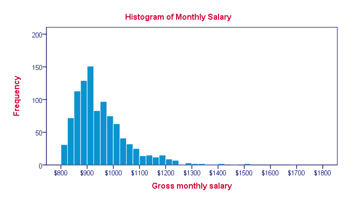 It is seen the variable of interest has a right skewed distribution.

Sample Histogram

It is seen the variable of interest has a right skewed distribution. ***

Re-sizing Images

You cannot arrange the size of image by using codes in R Markdown. However, It is able to change the size of images by adding some commands into your code chunks.

#The head of the chunk {r, out.width = "20%"} knitr::include_graphics("http://www.adayogrenci.metu.edu.tr/ankara/system/files/cover/hakkimizda_cover.jpg")

‘our.width’ helps to arrage the size of the image. In addition to this, there are other options used to re-size image. The following list shows the code used for images in R Markdown.

knitr::include_graphics("images.png")

Command List for re-sizing

This calls an R command included in the knitr package, with some options about how the R is run (described below).

Including Code and Comments

Code chunks are where the magic happens in R Markdown. The code you enter gets executed and the results are shown in the document.The code comes in two varieties, code chunks and inline code.

Code Chunks and Their Results

A code chunk is simply an off-set piece of code by itself. It is preceded by ```{r} on a line by itself, and ended by a line which just says ```. In order to add a chunk, click on

Then, select a chunk related to your codes

The code itself goes in between. Here, for instance, is some code which loads a data set from a library, and makes a scatter plot.

plot(cars$speed,cars$dist)

After the chunk, you can add your comment related to output.

First, notice how the code is included, nicely formatted, in the document. Second, notice how the output of the code is also automatically included in the document. If your code outputs numbers or text, those can be included too:

cor(cars$speed,cars$dist)

## [1] 0.8068949

Inline Code

Code output can also be seamlessly incorporated into the text, using inline code. This is code not set off on a line by itself, but beginning with `r and ending with `. Using inline code is how this document knows that the cars data set contains rows (contains 50 rows), and that the median distance of cars 36 equals to (36).

Notice that inline code does not display the commands run, just their output.

Chunk Options

There are many options in code chunks ( not inline codes) that enables us to modify apperance of output, codes and messages and warnings related to codes. Here, you can see these options. Notice that these options go after the initial r and before the closing } that announces the start of a code chunk.

This option does not show the codeS, only shows the results alone.

```{r, echo=FALSE}

Another option does not show neither the text of the code nor its output.

```{r, include=FALSE}

This might seem pointless, but it can be useful for code chunks which do set-up like loading data files, or initial model estimates, etc.

Another option prints the code in the document, but does not run it

```{r, eval=FALSE}

This is useful if you want to talk about the (nicely formatted) code.

The following option does not print the messages related to codes that you write in the chunk.

```{r, message=FALSE}

This option does not show the warnings related to codes you write in the chunk.

```{r, warning=FALSE}

Giving Chunk Names

It can be given chunk names easily after opening the chunk with the following structre.

```{r, nameofchunk}.

This name is then used for the images (or other files) that are generated when the document is rendered.

Default settings for including images and figures and Changing Image Sizes and Alignments in R Markdown

The table below shows some commonly-used settings from the rmarkdown and knitr packages and their corresponding default values. All settings shown below except for out.width and out.height will default to the rmarkdown value if left blank (rmarkdown does not have settings for out.width and out.height)

Image Sizes

Including images and figures

We include external images in our R markdown documents using the include_graphics function from the knitr package. Images can also be included using either raw HTML with img tags

(<img src = "" />)

or using markdown directly

().

We are using include_graphics for two reasons. First, the function is document format agnostic - meaning it can work with LaTeX or Markdown documents. Second, although you can technically include an image in a markdown document using standard HTML image tags

(<img src = "" />)

,using include_graphics will respect image settings listed in the R chunks like out.width and out.height.

How to use this command

The include_graphics command is used as follows

knitr::include_graphics("download.png")

Changing Image Sizes and Alignments

There are many options to control the size of the images. The most commonly used one fig.width, fig.height, out.height, out.width. By using fig family commands, you can arrange the size of image in terms of inches.

{r,fig.width=4}

However, by using out family commands, you can arrange the size of image in terms of percentage.

{r,out.width=%20}

There are a bunch of options for adjusting the placement of the figures which R produces. fig.align controls the horizontal alignment (left, right, or center).

When producing PDF, the options out.height and out.width let you specify the desired height or width of the figure, in inches, centimeters, or multiples of pre-defined lengths (from LaTeX). So for instance ```{r, out.height="3in"} forces the image to be 3 inches high, while ```{r, out.width="0.48\\textwidth"} forces the image’s width to be a bit less than half of the total width of the text on the page (so that two such images will fit side by side). The next few figures illustrate.

Tables

The default print-out of matrices, tables, etc. from R Markdown is frankly ugly. The knitr package contains a very basic command, kable, which will format an array or data frame more nicely for display.

Compare:

summary(cars)

## speed dist ## Min. : 4.0 Min. : 2.00 ## 1st Qu.:12.0 1st Qu.: 26.00 ## Median :15.0 Median : 36.00 ## Mean :15.4 Mean : 42.98 ## 3rd Qu.:19.0 3rd Qu.: 56.00 ## Max. :25.0 Max. :120.00

with

library(knitr) # Only need this the first time! kable(summary(cars))

speed dist

Min. : 4.0 Min. : 2.00

1st Qu.:12.0 1st Qu.: 26.00

Median :15.0 Median : 36.00

Mean :15.4 Mean : 42.98

3rd Qu.:19.0 3rd Qu.: 56.00

Max. :25.0 Max. :120.00

— Of course, R’s defaults print out a crazy number of decimal places, but this isn’t the time to discuss significant digits, or the signif function.

“Caching” Code Chunks (Re-Running Only When Changed)

By default, R Markdown will re-run all of your code every time you render your document. If some of your code is slow, this can add up to a lot of time. You can, however, ask R Markdown to keep track of whether a chunk of code has changed, and only re-run it if it has. This is called caching the chunk.

plot(cars$speed,cars$dist)

One issue is that a chunk of code which hasn’t changed itself might call on results of earlier, modified chunks, and then we would want to re-run the downstream chunks. There are options for manually telling R Markdown “this chunk depends on this earlier chunk”, but it’s generally easier to let it take care of that, by setting the autodep=TRUE option.

1. If you load a package with the library() or require() commands, R Markdown isn’t smart enough to check whether the package has changed (or indeed been installed, if you were missing it). So that won’t trigger an automatic re-running of a cached code chunk.

2. To manually force re-running all code chunks, the easiest thing to do is to delete the directory R Markdown will create (named something like filename_cache) which it uses to store the state of all code chunks.

Setting Defaults for All Chunks

You can tell R to set some defaults to apply to all chunks where you don’t specifically over-ride them. Here are the ones I generally use:

# Need the knitr package to set chunk options library(knitr) # Set knitr options for knitting code into the report: # - Don't print out code (echo) # - Save results so that code blocks aren't re-run unless code changes (cache), # _or_ a relevant earlier code block changed (autodep), but don't re-run if the # only thing that changed was the comments (cache.comments) # - Don't clutter R output with messages or warnings (message, warning) # This _will_ leave error messages showing up in the knitted report opts_chunk$set(echo=FALSE, cache=TRUE, autodep=TRUE, cache.comments=FALSE, message=FALSE, warning=FALSE)

This sets some additional options beyond the ones I’ve discussed, like not re-running a chunk if only the comments have changed (cache.comments = FALSE), and leaving out messages and warnings. (I’d only recommend suppressing warnings once you’re sure your code is in good shape.) I would typically give this set-up chunk itself the option include=FALSE.

You can over-ride these defaults by setting options for individual chunks.

More Options

See [http://yihui.name/knitr/options/] for a complete listing of possible chunk options.

Math in R Markdown

Since this is a statistics class, you need to be able to write out mathematical expressions, often long series of them. R Markdown gives you the syntax to render complex mathematical formulas and derivations, and have them displayed very nicely. Like code, the math can either be inline or set off (displays).

Inline math is marked off witha pair of dollar signs ($), as 𝜋𝑟2 or 𝑒𝑖𝜋.

Inline math is marked off witha pair of dollar signs (`$`), as $\pi r^2$ or $e^{i\pi}$.

Mathematical displays are marked off with \[ and \], as in

𝑒𝑖𝜋 = −1

Mathematical displays are marked off with `\[` and `\]`, as in \[ e^{i \pi} = -1 \]

Once your text has entered math mode, R Markdown turns over the job of converting your text into math to a different program, called LaTeX[^latex]. This is the most common system for typesetting mathematical documents throughout the sciences, and has been for decades. It is extremely powerful, stable, available on basically every computer, and completely free. It is also, in its full power, pretty complicated. Fortunately, the most useful bits, for our purposes, are actually rather straightforward.

Elements of Math Mode • Most letters will be rendered in italics (compare: a vs. a vs. 𝑎; only the last is in math

mode). The spacing between letters also follows the conventions for math, so don’t treat it as just another way of getting italics. (Compare speed, in simple italics, with 𝑠𝑝𝑒𝑒𝑑, in math mode.)

• Greek letters can be accessed with the slash in front of their names, as \alpha for 𝛼. Making the first letter upper case gives the upper-case letter, as in \Gamma for 𝛤 vs. \gamma for 𝛾. (Upper-case alpha and beta are the same as Roman A and B, so no special commands for them.)

• There are other “slashed” (or “escaped”) commands for other mathematical symbols:

– \times for ×

– \cdot for ⋅

– \leq and \geq for ≤ and ≥

– \subset and \subseteq for ⊂ and ⊆

– \leftarrow, \rightarrow, \Leftarrow, \Rightarrow for ←, →, ⇐, ⇒

– \approx, \sim, \equiv for ≈, ∼, ≡

– See, e.g., http://web.ift.uib.no/Teori/KURS/WRK/TeX/symALL.html for a fuller listing of available symbols. (http://tug.ctan.org/info/symbols/comprehensive/symbols-a4.pdf lists all symbols available in LaTeX, including many non-mathematical special chracters)

• Subscripts go after an underscore character, _, and superscripts go after a caret, ^, as \beta_1 for 𝛽1 or a^2 for 𝑎2.

• Curly braces are used to create groupings that should be kept together, e.g., a_{ij} for 𝑎𝑖𝑗 (vs. a_ij for 𝑎𝑖𝑗).

• If you need something set in ordinary (Roman) type within math mode, use \mathrm, as t_{\mathrm{in}}^2 for 𝑡in

2 .

• If you’d like something set in an outline font (“blackboard bold”), use \mathbb, as \mathbb{R} for ℝ.

• For bold face, use \mathbf, as

(\mathbf{x}^T\mathbf{x})^{-1}\mathbf{x}^T\mathbf{y}

for

(𝐱𝑇𝐱)−1𝐱𝑇𝐲

• Accents on characters work rather like changes of font: \vec{a} produces �⃗⃗� , \hat{a}

produces �̂�. Some accents, particularly hats, work better if they space out, as with

\widehat{\mathrm{Var}} producing Varˆ .

• Function names are typically written in romans, and spaced differently: thus log𝑥, not 𝑙𝑜𝑔𝑥. LaTeX, and therefore R Markdown, knows about a lot of such functions, and their names all begin with \. For instance: \log, \sin, \cos, \exp, \min, etc. Follow these function names with the argument in curly braces; this helps LaTeX figure out what exactly the argument is, and keep it grouped together with the function name when it’s laying out the text. Thus \log{(x+1)} is better than \log (x+1).

• Fractions can be created with \frac, like so:

\frac{a+b}{b} = 1 + \frac{a}{b}

produces 𝑎 + 𝑏

𝑏= 1 +

𝑎

𝑏

• Sums can be written like so:

\sum_{i=1}^{n}{x_i^2}

will produce

∑𝑥𝑖2

𝑛

𝑖=1

The lower and upper limits of summation after the \sum are both optional. Products and integrals work similarly, only with \prod and \int:

𝑛! = ∏𝑖

𝑛

𝑖=1

log𝑏 − log𝑎 = ∫1

𝑥𝑑𝑥

𝑥=𝑏

𝑥=𝑎

\sum, \prod and \int all automatically adjust to the size of the expression being summed, producted or integrated.

• “Delimiters”, like parentheses or braces, can automatically re-size to match what they’re surrounding. To do this, you need to use \left and \right, as

\left( \sum_{i=1}^{n}{i} \right)^2 = \left( \frac{n(n-1)}{2}\right)^2 = \frac{n^2(n-1)^2}{4}

renders as

( ∑𝑛

𝑖=1𝑖)

2

= (𝑛(𝑛 − 1)

2)2

=𝑛2(𝑛 − 1)2

4

• To use curly braces as delimiters, precede them with slashes, as \{ and \} for { and }.

• Multiple equations, with their equals signs lined up, can be created using eqnarray, as follows.

\[ \begin{eqnarray} X & \sim & \mathrm{N}(0,1)\\ Y & \sim & \chi^2_{n-p}\\ R & \equiv & X/Y \sim t_{n-p} \end{eqnarray} \]

𝑋 ∼ N(0,1)

𝑌 ∼ 𝜒𝑛−𝑝2

𝑅 ≡ 𝑋/𝑌 ∼ 𝑡𝑛−𝑝

Notice that & surrounds what goes in the middle on each line, and each line (except the last) is terminated with \\. The left or right hand side of the equation can be blank, and space will be made:

\[ \begin{eqnarray} P(|X-\mu| > k) & = & P(|X-\mu|^2 > k^2)\\ & \leq & \frac{\mathbb{E}\left[|X-\mu|^2\right]}{k^2}\\ & \leq & \frac{\mathrm{Var}[X]}{k^2} \end{eqnarray} \]

𝑃(|𝑋 − 𝜇| > 𝑘) = 𝑃(|𝑋 − 𝜇|2 > 𝑘2)

≤𝔼[|𝑋 − 𝜇|2]

𝑘2

≤Var[𝑋]

𝑘2

(In full LaTeX, \begin{eqnarray} automatically enters math mode, but R Markdown needs the hint.)

Translating Math into LaTeX

LaTeX is designed so that every part of a mathematical expression has a reasonably straightforward counterpart in what you write. Still, it can be a bit intimidating at first. What many people find useful to to start by taking some page of printed or hand-written math and then deliberately translate that, line by line, into LaTeX, and then rendering it to see whether it came out right (and, if not, where to fix things). If you need to do any math for an assignment, it can be a good idea to write the math out by hand, and then turn it into LaTeX, whether the class requires it (like this one) or not. Eventually, with practice, the translation will become quite automatic, and some people even do new math by writing out the LaTeX.

LaTeX Does Not Check Correctness

LaTeX does not check whether your math is right; it just checks whether it can figure out what you’re trying to say well enough to type-set it. Thus for instance it has no problem at all with the following:

(𝑛 + 1)(𝑛 − 1) = 𝑛2

𝑛2 − 1 = 𝑛2

−1 = 01 = 0

−1 = 1

(There are computer programs for doing symbolic mathematics which, in effect, do check whether your math is right, at least if you’re working in the sub-area of math they’re designed to handle. So far as I know, no one has ever really combined them with LaTeX.)

More Advanced Math-Mode Stuff: New Commands

One of the things you can do in LaTeX is create your own commands. This is useful if you find yourself writing out the same complicated expression repeatedly, or, alternatively, if you want to make sure that the same symbol is always used for the same concept. For

instance, in some areas of statistics, the generic parameter of a model is 𝜃, in others 𝛽, in yet others 𝜓. If you do something like this early on

\[ \newcommand{\MyParameter}{\theta} \]

then in later bits of math mode you can write \MyParameter, and LaTeX will translate this to \theta. If you later decide that you want your parameter to be \beta, or even \mathrm{fred}, you just change that initial definition of the new command, rather than having to track down each \theta.

New commands can also take one or more arguments. Here is a useful command for writing expectations:

\[ \newcommand{\Expect}[1]{\mathbb{E}\left[ #1 \right]} \]

And here is a command for writing covariances:

\[ \newcommand{\Cov}[2]{\mathrm{Cov}\left[ #1, #2\right]} \]

Defining commands like this not only saves you typing, and makes it easier to make changes; it also makes your math-mode text easier for you, or others, to read even if it isn’t rendered. This is like using comprehensible variable and function names in your programs, and for that matter like using functions rather than long strings of commands in the first place.

It is also possible to define new function names which act like \log, new mathematical operators, draw diagrams, etc., etc., but that goes way beyond the scope of these notes.

Installing LaTeX

If you render your R Markdown document to HTML, you do not need to install LaTeX on your computer. This is because the HTML includes instructions to browsers, which say (as it were) “Send the funny-looking bits with all the slashes to mathjax.org, and it will send you back pretty pictures of equations”. The website actually runs the LaTeX.

If you want to produce PDF, you need to have LaTeX installed on your computer. How you actually do this depends on the precise kind of computer. For Macs, I recommend using the MacTeX package, available from https://tug.org/mactex/mactex-download.html. For other systems, follow the links from http://www.tug.org/begin.html.

Putting It All Together: Writing Your Report in R Markdown • You have installed the rmarkdown package and all its dependencies.

• You have installed LaTeX, if you’re producing a PDF.

• You have installed and fired up your favorite text editor.

• You open it up to a new document.

– You give it a title, an author, and a date.

• You use headers to divide it into appropriate, titled sections, and possibly sub-sections.

– One common pattern: “Introduction”, “Data and Research Questions”, “Analysis”, “Results”, “Conclusion”.

– Another common pattern: “Problem 1”, “Problem 2”, … , “Extra Credit”.

• You write text.

• When you need it, you insert math into the text, or even whole mathematical displays.

• When you need it, you insert code into your document.

– The code runs (as needed) when you render the document.

– Figures, tables, and other output are automatically inserted into the document, and track changes in your code.

• Every so often, try to render your document.

– When you (think you) have finished a section is a good time to do so.

– Another good time is once you’ve made any non-trivial change to the code or the text.

• Either your document rendered successfully or it didn’t.

– If it did, and you like the results, congratulate yourself and cheerfully go on to your next task.

– If it rendered but you don’t like the results, think about why and try to fix it.

– If it didn’t render, R will tell you where it gave up, so try to debug from around there.

Troubleshooting/Stuff to Avoid • Do not call View or help in your document; these are interactive commands which

don’t work well in scripts.

• “It worked in the console but it wouldn’t knit”: You have almost certainly done something somewhat different before the code chunk that’s giving you trouble. Clear your workspace in the console and re-run.

– R Studio keeps two environments or workspaces which it uses to evaluate R expressions, look up function or variable names, etc. One is the “usual” global environment of the console, which builds cumulatively from the start of your session. (Unless you deliberately manipulate it; don’t do that unless you know what you’re doing.) Every time you knit, however, it re-runs your code in clean workspace, as though you had just started R from scratch. This means knitted

code does what you say it should, and only that. If your code knits, it should work on any computer; getting something to run in the console which you can’t reproduce is just dumb luck.

• “It works when I source it, but it won’t knit”: This is basically the same problem as “it worked in the console”.

• Avoid attach in both the console and in your file; using it is a recipe for creating hard-to-find errors. You can still shorten expressions using with instead.

• You need LaTeX to create PDFs. If you are having trouble doing so, try switching the output format to HTML.

– Do try to fix your LaTeX installation later, when you don’t have such time pressure; it’s really useful.

– LaTeX will complain if you try to print out truly enormous things. Errors about “out of stack”, or “pandoc 43”, are often caused by this. Don’t print out enormous things. (Suppressing warnings and other messages may help.)

• When you need to load data files or source someone else’s code, use full URLs, rather than creating local copies and loading them from your disk.