Mark Watson Slides - FGV EPGE
61
Last revised 5/9/2013 1 Inference in Structural VARs with External Instruments José Luis Montiel Olea, Harvard University (NYU) James H. Stock, Harvard University Mark W. Watson, Princeton University 3rd VALE-EPGE Global Economic Conference “Business Cycles” May 9-10, 2013
Transcript of Mark Watson Slides - FGV EPGE

Last revised 5/9/2013 1
Inference in Structural VARs with External Instruments
José Luis Montiel Olea, Harvard University (NYU) James H. Stock, Harvard University
Mark W. Watson, Princeton University
3rd VALE-EPGE Global Economic Conference “Business Cycles” May 9-10, 2013
Last revised 5/9/2013 2
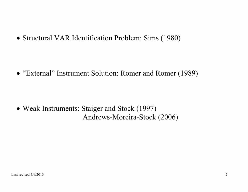
Structural VAR Identification Problem: Sims (1980)
“External” Instrument Solution: Romer and Romer (1989)
Weak Instruments: Staiger and Stock (1997)
Andrews-Moreira-Stock (2006)

Last revised 5/9/2013 3
Notation
Reduced form VAR: Yt = A(L)Yt—1 + ηt ;
A(L) = A1L + + ApLp;
Y is r ×1
Structural Shocks: ηt = Ht = 1
1
t
r
rt
H H
, H is non-singular.
Structural VAR: Yt = A(L)Yt—1 + Ht
Structural MA: Yt = [I−A(L)]−1Ht = C(L)Ht
C(L)H is structural impulse response function (dynamic causal effect)
Last revised 5/9/2013 4
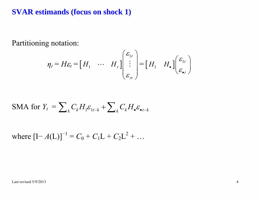
SVAR estimands (focus on shock 1) Partitioning notation:
ηt = Ht = 1
1
t
r
rt
H H
= 11
t
t
H H
SMA for Yt = 1 1k t k k t kk k
C H C H where [I− A(L)]−1 = C0 + C1L + C2L2 + …

Last revised 5/9/2013 5
SVAR estimands: Write SMA for Yt = 1 1k t k k t kk k
C H C H
Impulse Resp: IRFj,k = 1
jt
t k
Y
= Cj,kH1 , where Cj,k is the j’th row of Ck
Historical Decomposition: HDj,k = , 1 10
kj l t ll
C H
Variance Decomposition: VDj,k = , 1 10
,0
var
var
kj l t ll
kj l t ll
C H
C

Last revised 5/9/2013 6
Two approaches for structural VAR identification problem: = H
1. Internal restrictions: Short run restrictions (Sims (1980)), long run restrictions, identification by heteroskedasticity, bounds on IRFs)
2. External information (“method of external instruments”): Romer and Romer (1989), Ramey and Shapiro (1998), … Selected empirical papers Monetary shock: Cochrane and Piazzesi (2002), Faust, Swanson, and Wright
(2003. 2004), Romer and Romer (2004), Bernanke and Kuttner (2005), Gürkaynak, Sack, and Swanson (2005)
Fiscal shock: Romer and Romer (2010), Fisher and Peters (2010), Ramey (2011)
Uncertainty shock: Bloom (2009), Baker, Bloom, and Davis (2011), Bekaert, Hoerova, and Lo Duca (2010), Bachman, Elstner, and Sims (2010)
Liquidity shocks: Gilchrist and Zakrajšek’s (2011), Bassett, Chosak, Driscoll, and Zakrajšek’s (2011)
Oil shock: Hamilton (1996, 2003), Kilian (2008a), Ramey and Vine (2010)
Last revised 5/9/2013 7
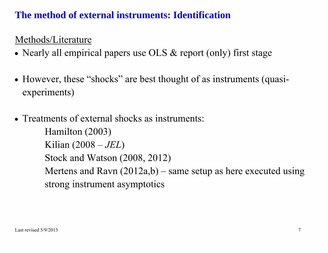
The method of external instruments: Identification Methods/Literature Nearly all empirical papers use OLS & report (only) first stage
However, these “shocks” are best thought of as instruments (quasi-
experiments)
Treatments of external shocks as instruments: Hamilton (2003) Kilian (2008 – JEL) Stock and Watson (2008, 2012) Mertens and Ravn (2012a,b) – same setup as here executed using strong instrument asymptotics
Last revised 5/9/2013 8
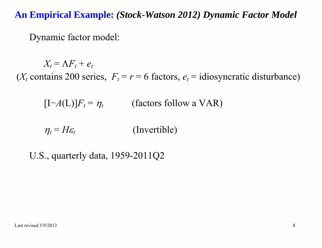
An Empirical Example: (Stock-Watson 2012) Dynamic Factor Model
Dynamic factor model:
Xt = Ft + et (Xt contains 200 series, Ft = r = 6 factors, et = idiosyncratic disturbance)
[I−A(L)]Ft = t (factors follow a VAR) t = Ht (Invertible)
U.S., quarterly data, 1959-2011Q2
Last revised 5/9/2013 9
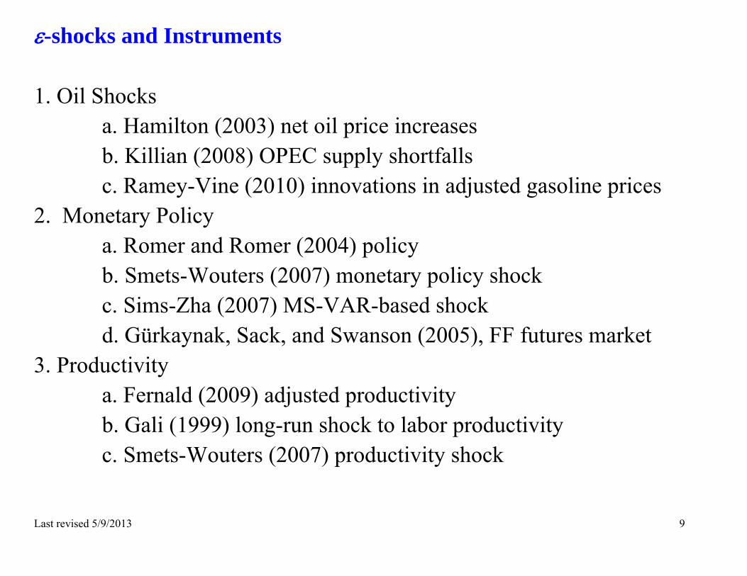
-shocks and Instruments 1. Oil Shocks
a. Hamilton (2003) net oil price increases b. Killian (2008) OPEC supply shortfalls c. Ramey-Vine (2010) innovations in adjusted gasoline prices
2. Monetary Policy a. Romer and Romer (2004) policy b. Smets-Wouters (2007) monetary policy shock c. Sims-Zha (2007) MS-VAR-based shock d. Gürkaynak, Sack, and Swanson (2005), FF futures market
3. Productivity a. Fernald (2009) adjusted productivity b. Gali (1999) long-run shock to labor productivity c. Smets-Wouters (2007) productivity shock
Last revised 5/9/2013 10
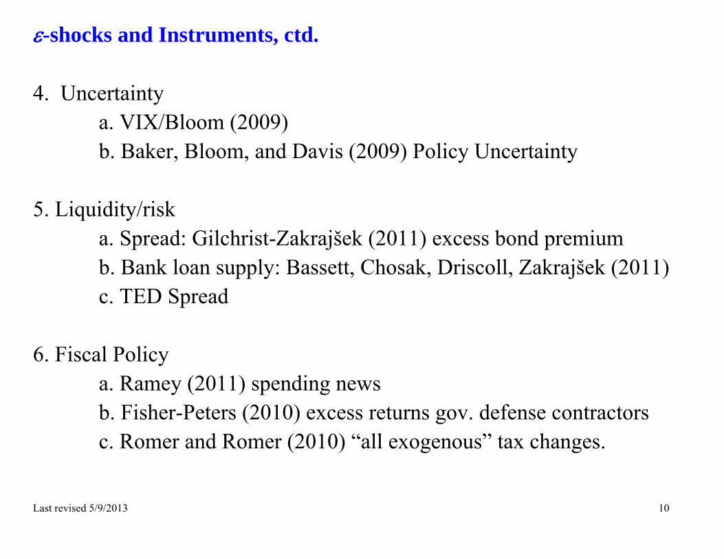
-shocks and Instruments, ctd. 4. Uncertainty a. VIX/Bloom (2009) b. Baker, Bloom, and Davis (2009) Policy Uncertainty 5. Liquidity/risk a. Spread: Gilchrist-Zakrajšek (2011) excess bond premium b. Bank loan supply: Bassett, Chosak, Driscoll, Zakrajšek (2011)
c. TED Spread 6. Fiscal Policy a. Ramey (2011) spending news b. Fisher-Peters (2010) excess returns gov. defense contractors c. Romer and Romer (2010) “all exogenous” tax changes.
Last revised 5/9/2013 11
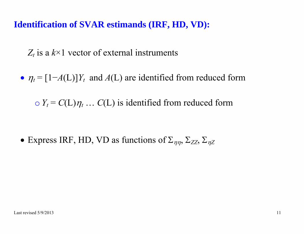
Identification of SVAR estimands (IRF, HD, VD):
Zt is a k×1 vector of external instruments
t = [1−A(L)]Yt and A(L) are identified from reduced form
o Yt = C(L)t … C(L) is identified from reduced form
Express IRF, HD, VD as functions of , ZZ, Z
Last revised 5/9/2013 12
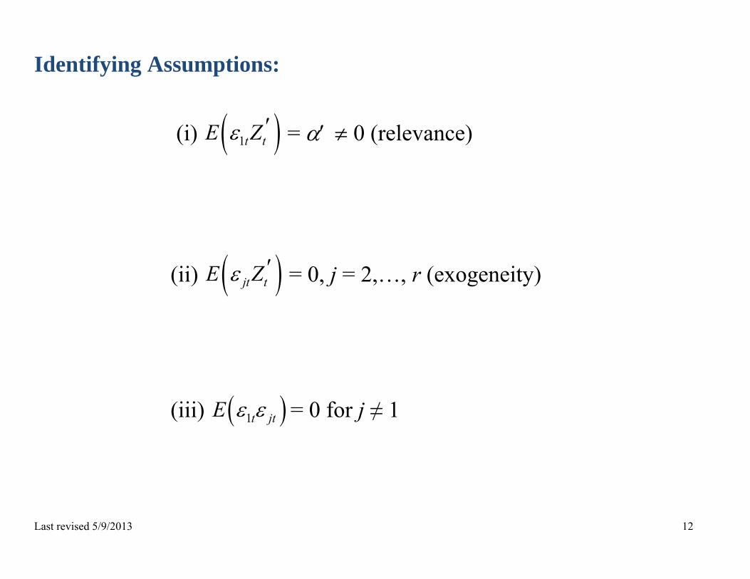
Identifying Assumptions:
(i) 1t tE Z = 0 (relevance)
(ii) jt tE Z = 0, j = 2,…, r (exogeneity)
(iii) 1t jtE
= 0 for j ≠ 1

Last revised 5/9/2013 13
Identification of IRFj,k = Cj,kH1
Z = E(tZt) = E(HtZt) = 1
1
( )
( )
t t
r
rt t
E ZH H
E Z
= 1 00
rH H
= H1
Normalization: The scale of H1 and 1
2 is set by a normalization, The
normalization used here: a unit positive value of shock 1 is defined to have a unit positive effect on the innovation to variable 1, which is u1t. This corresponds to:
(iv) H11 = 1 (unit shock normalization)
where H11 is the first element of H1

Last revised 5/9/2013 14
Identification of IRFj,k = Cj,kH1, ctd Z = H1so H1 = Z/(’)
Impose normalization (iv):
Z = H1 11
1
HH
1
1H
so ꞌ = 1Z
and H1 = Z 1Z /(
1Z 1Z )
If Zt is a scalar (k = 1): H1 = 1 t
t
t
t
E ZE Z

Last revised 5/9/2013 15
Identification of HD = , 1 10
h
k j t jk
C H requires identification of H11t
Proj(Zt | t) = Proj(Zt | t) = Proj(Zt | 1t) = b1t where b=1
2
t
H11t = Proj(t | 1t) = Proj(t | b1t) = Proj(t | Proj(Zt | t)) = Proj(t | Z
1 t)
= 1
t,
where = Z(Z
1 Z Z)+
(Note Z = ’H1 has rank 1, so pseudo inverse is used)

Last revised 5/9/2013 16
Identification of VD = , 1 10
,0
var
var
kj l t ll
kj l t ll
C H
C
Note this requires identification of var(H11t), which from last slide is var( 1
t) = 1
ꞌ.
Last revised 5/9/2013 17
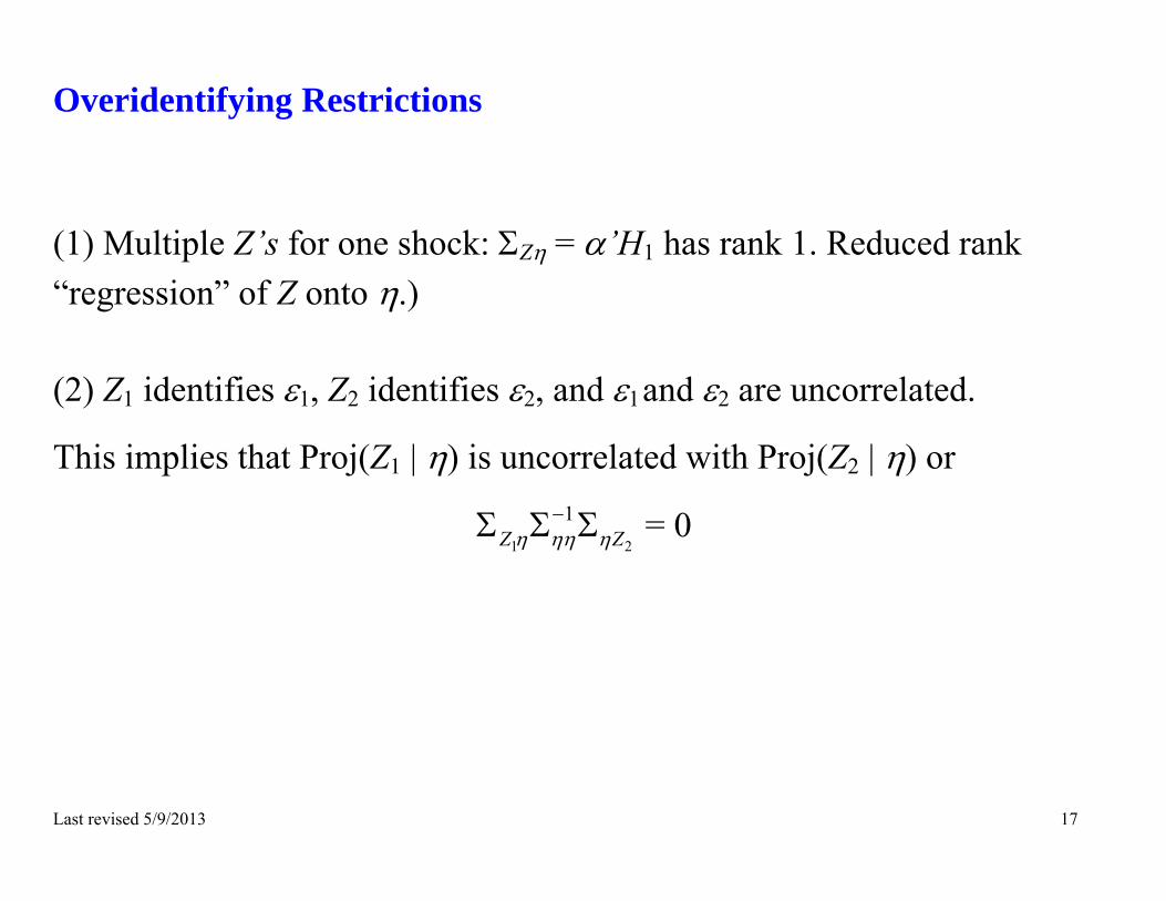
Overidentifying Restrictions (1) Multiple Z’s for one shock: Z = ’H1 has rank 1. Reduced rank “regression” of Z onto .) (2) Z1 identifies 1, Z2 identifies 2, and 1 and 2 are uncorrelated.
This implies that Proj(Z1 | ) is uncorrelated with Proj(Z2 | ) or
1 2
1Z Z
= 0
Last revised 5/9/2013 18
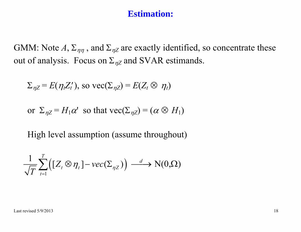
Estimation:
GMM: Note A, , and Z are exactly identified, so concentrate these out of analysis. Focus on Z and SVAR estimands.
Z = E(tZt), so vec(Z) = E(Zt t) or Z = H1ꞌ so that vec(Z) = ( H1)
High level assumption (assume throughout)
1
1 [ ] ( )T
t t Zt
Z vecT
d N(0,)
Last revised 5/9/2013 19
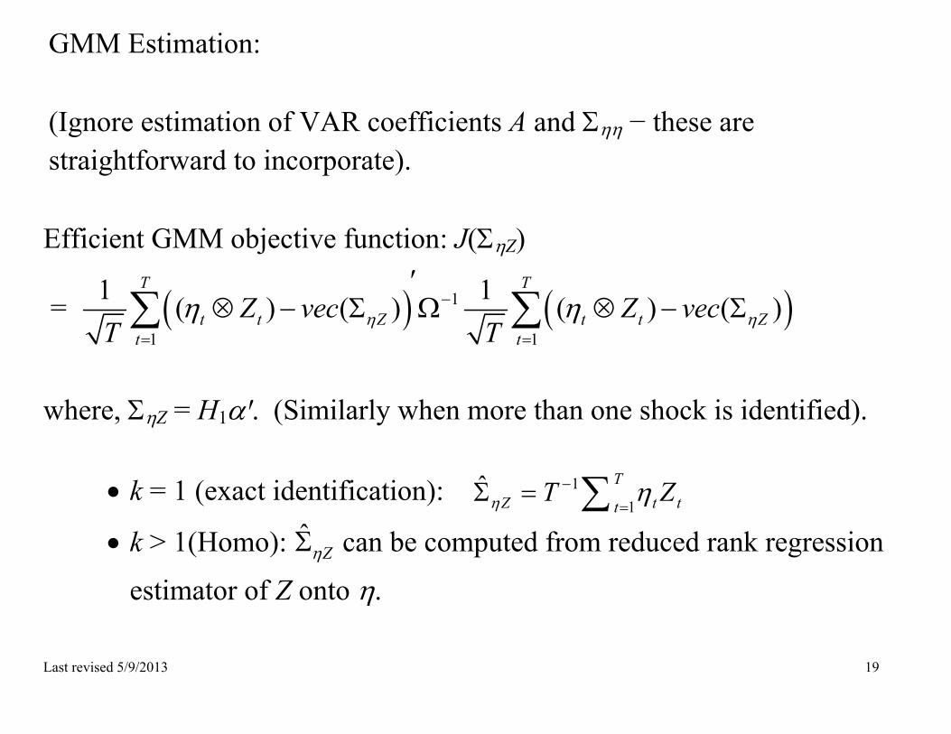
GMM Estimation: (Ignore estimation of VAR coefficients A and − these are straightforward to incorporate). Efficient GMM objective function: J(Z)
= 1
1 1
1 1( ) ( ) ( ) ( )T T
t t Z t t Zt t
Z vec Z vecT T
where, Z = H1ꞌ. (Similarly when more than one shock is identified).
k = 1 (exact identification): 11
ˆ TZ t tt
T Z
k > 1(Homo): ˆZ can be computed from reduced rank regression
estimator of Z onto .
Last revised 5/9/2013 20
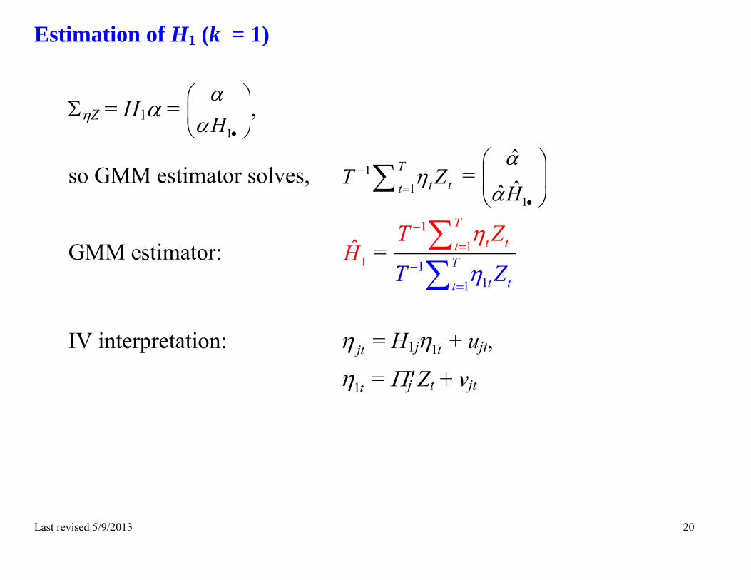
Estimation of H1 (k = 1)
Z = H1= 1H
,
so GMM estimator solves, 11
Tt tt
T Z =
1
ˆˆˆH
GMM estimator: 1H = 1
1
1
11
Tt t
t
tT
ttT
Z
Z
T
IV interpretation: jt = H1j 1t + ujt,
1t = jZt + vjt
Last revised 5/9/2013 21
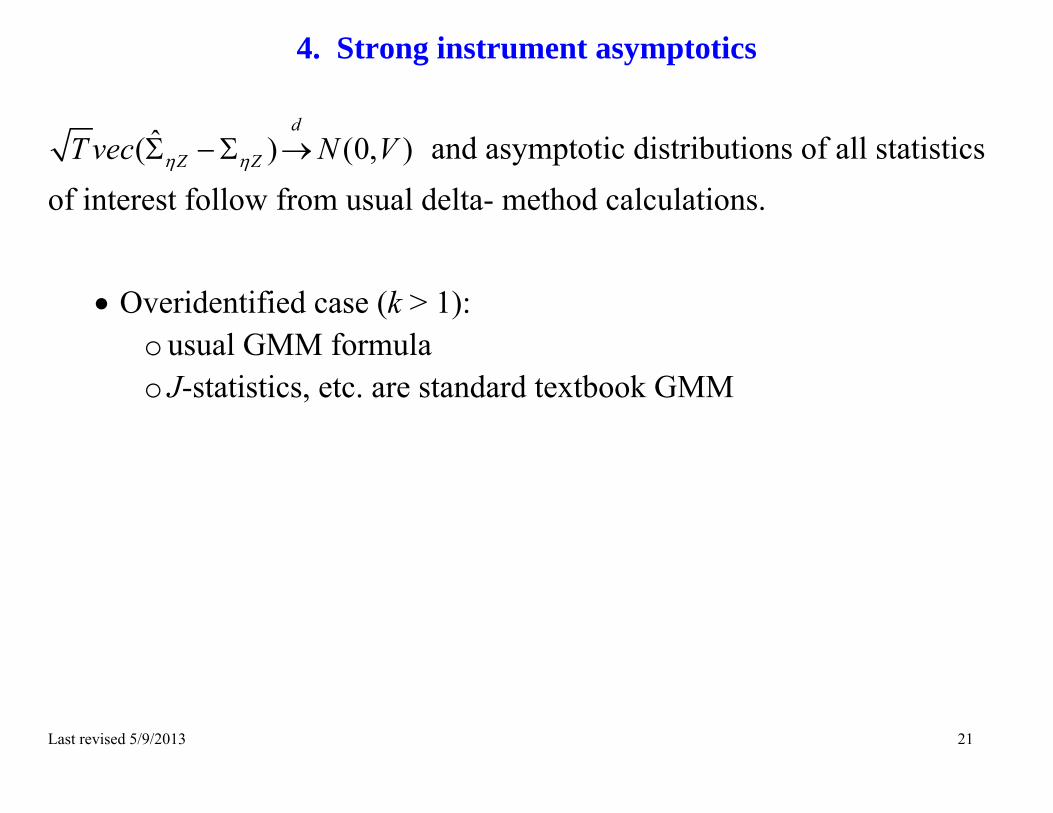
4. Strong instrument asymptotics
ˆ( ) (0, )d
Z ZT vec N V and asymptotic distributions of all statistics of interest follow from usual delta- method calculations.
Overidentified case (k > 1):
o usual GMM formula o J-statistics, etc. are standard textbook GMM
Last revised 5/9/2013 22
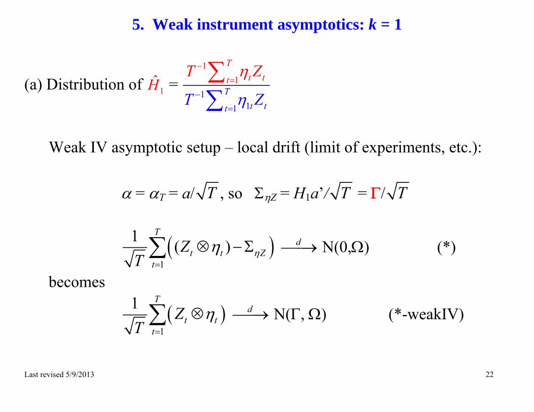
5. Weak instrument asymptotics: k = 1
(a) Distribution of 1H = 1
1
1
11
Tt t
t
tT
ttT
Z
Z
T
Weak IV asymptotic setup – local drift (limit of experiments, etc.):
= T = a/ T , so Z = H1a’/ T = / T
1
1 ( )T
t t Zt
ZT
d N(0,) (*)
becomes
1
1 T
t tt
ZT
d N(, ) (*-weakIV)

Last revised 5/9/2013 23
1
1 T
t tt
ZT
d N(, )
Weak instrument asymptotics for H1, ctd
1H = 1/2
11/2
11
Tt tt
Tt tt
T Z
T Z
Standardize (*):
1
1 1
1
1 T
Z t tt
ZT
+ z, (**)
where = 1
1 1Z and z ~ N(0,/(
1
2 2Z ) ),
Thus, in k = 1 case, 1H = 1
11
11
Tt tt
Tt tt
T Z
T Z
1 1
zz
= *1H
Last revised 5/9/2013 24
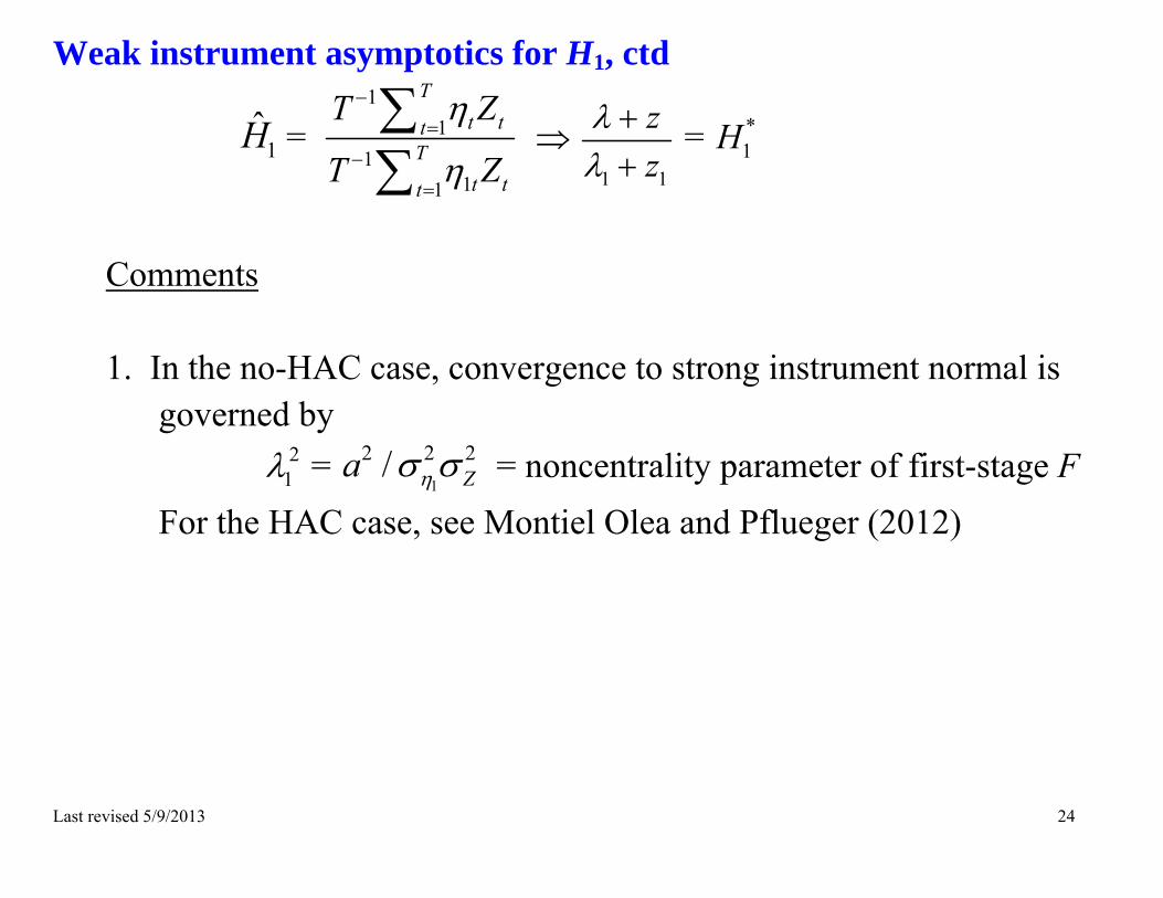
Weak instrument asymptotics for H1, ctd
1H = 1
11
11
Tt tt
Tt tt
T Z
T Z
1 1
zz
= *1H
Comments 1. In the no-HAC case, convergence to strong instrument normal is
governed by 2
1 = 1
2 2 2/ Za = noncentrality parameter of first-stage F For the HAC case, see Montiel Olea and Pflueger (2012)
Last revised 5/9/2013 25
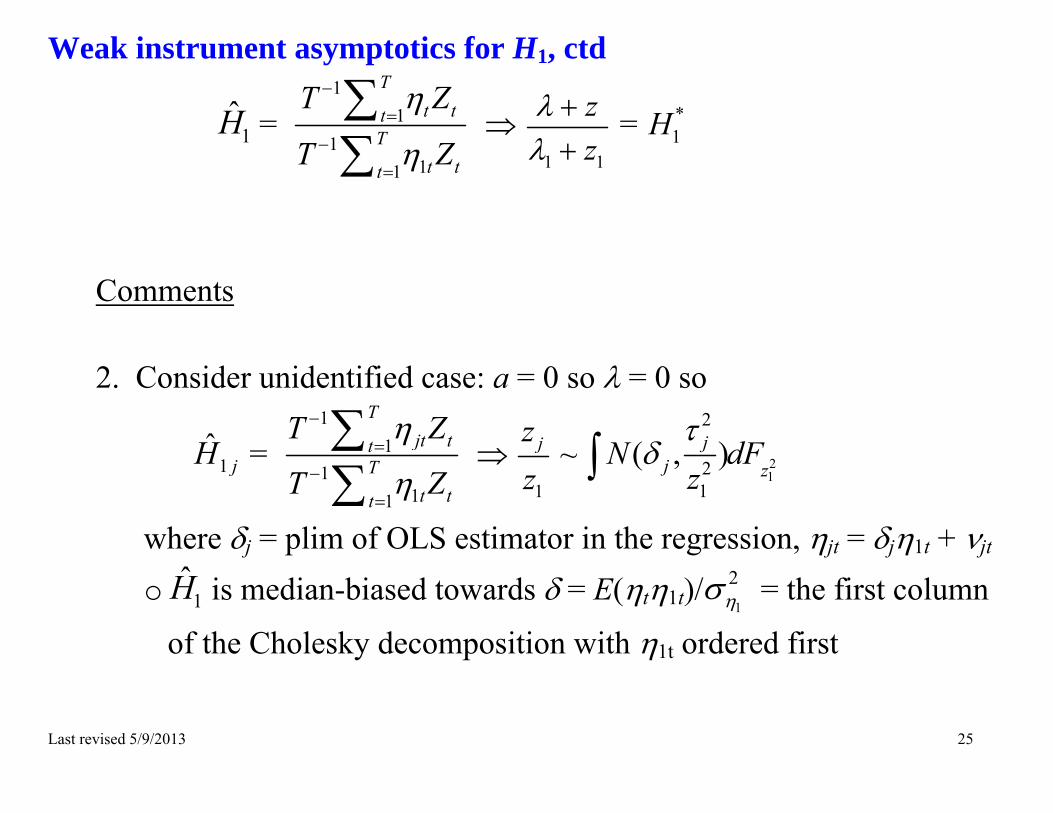
Weak instrument asymptotics for H1, ctd
1H = 1
11
11
Tt tt
Tt tt
T Z
T Z
1 1
zz
= *1H
Comments 2. Consider unidentified case: a = 0 so = 0 so
1ˆ
jH = 1
11
11
Tjt tt
Tt tt
T Z
T Z
1
jzz
~ 21
2
21
( , )jj z
N dFz
where j = plim of OLS estimator in the regression, jt = j1t + jt o 1H is median-biased towards = E(t1t)/ 1
2 = the first column
of the Cholesky decomposition with 1t ordered first
Last revised 5/9/2013 26
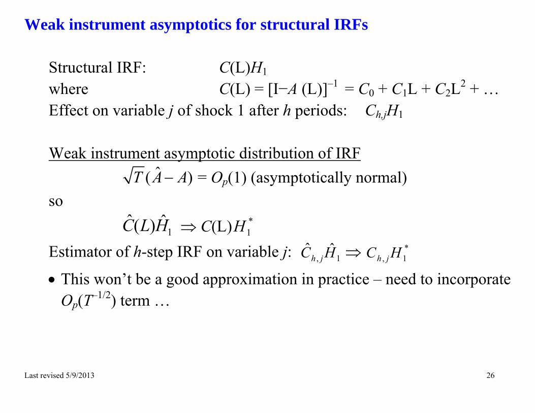
Weak instrument asymptotics for structural IRFs
Structural IRF: C(L)H1 where C(L) = [I−A (L)]–1
= C0 + C1L + C2L2 + … Effect on variable j of shock 1 after h periods: Ch,jH1 Weak instrument asymptotic distribution of IRF
ˆ( )T A A = Op(1) (asymptotically normal) so
1ˆ ˆ( )C L H C(L) *
1H Estimator of h-step IRF on variable j: , 1
ˆ ˆh jC H *
, 1h jC H
This won’t be a good approximation in practice – need to incorporate Op(T–1/2) term …

Last revised 5/9/2013 27
Numerical results for IRFs – asymptotic distributions DGP calibration: r = 2 Y = (lnPOILt, lnGDPt), US, 1959Q1-2011Q2 Estimate (L), , and H1, then fix throughout
o A(L), : VAR(2) o H1: estimated using Zt = Kilian (2008 – REStat) OPEC supply
shortfall (available 1971Q1-2004Q3)

Last revised 5/9/2013 28
Effect of oil on oil growth: 21 = 100
1 2 3 4 5 6 7 8 9 10 11 12−0.2
0
0.2
0.4
0.6
0.8
1
Quarter
Impulse:Oil; Response:OilCentrality Parameter=100
Last revised 5/9/2013 29
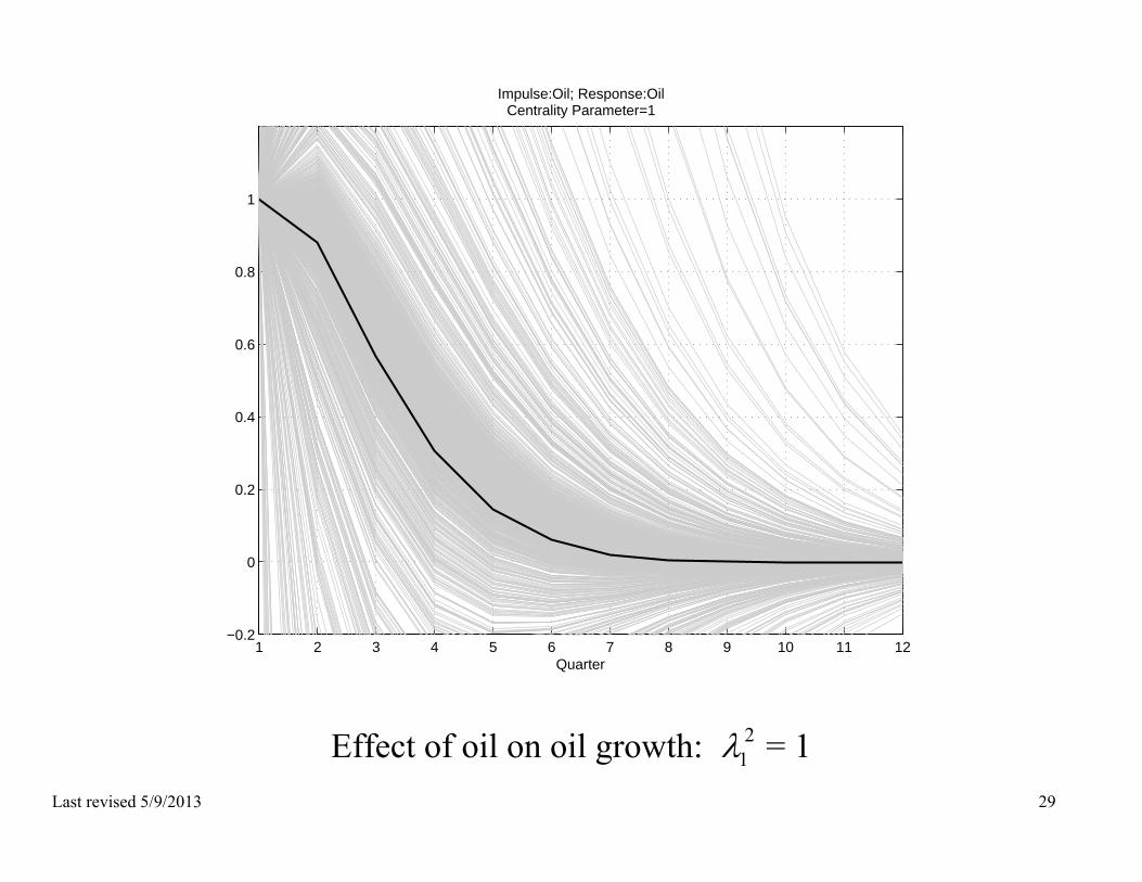
Effect of oil on oil growth: 21 = 1
1 2 3 4 5 6 7 8 9 10 11 12−0.2
0
0.2
0.4
0.6
0.8
1
Quarter
Impulse:Oil; Response:OilCentrality Parameter=1
Last revised 5/9/2013 30
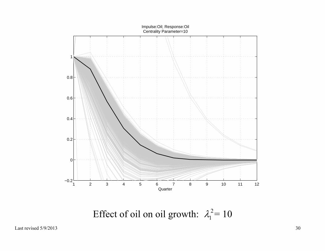
Effect of oil on oil growth: 21 = 10
1 2 3 4 5 6 7 8 9 10 11 12−0.2
0
0.2
0.4
0.6
0.8
1
Quarter
Impulse:Oil; Response:OilCentrality Parameter=10
Last revised 5/9/2013 31
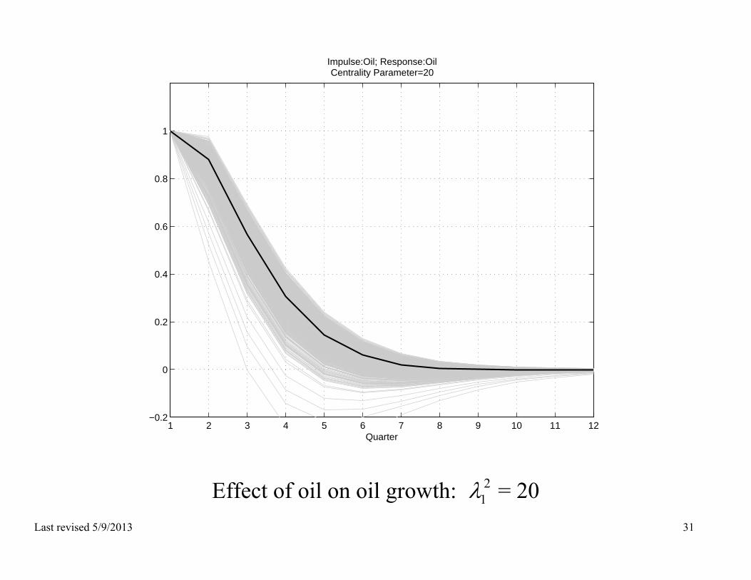
Effect of oil on oil growth: 21 = 20
1 2 3 4 5 6 7 8 9 10 11 12−0.2
0
0.2
0.4
0.6
0.8
1
Quarter
Impulse:Oil; Response:OilCentrality Parameter=20

Last revised 5/9/2013 32
Effect of oil on oil growth: 21 = 50
1 2 3 4 5 6 7 8 9 10 11 12−0.2
0
0.2
0.4
0.6
0.8
1
Quarter
Impulse:Oil; Response:OilCentrality Parameter=50
Last revised 5/9/2013 33
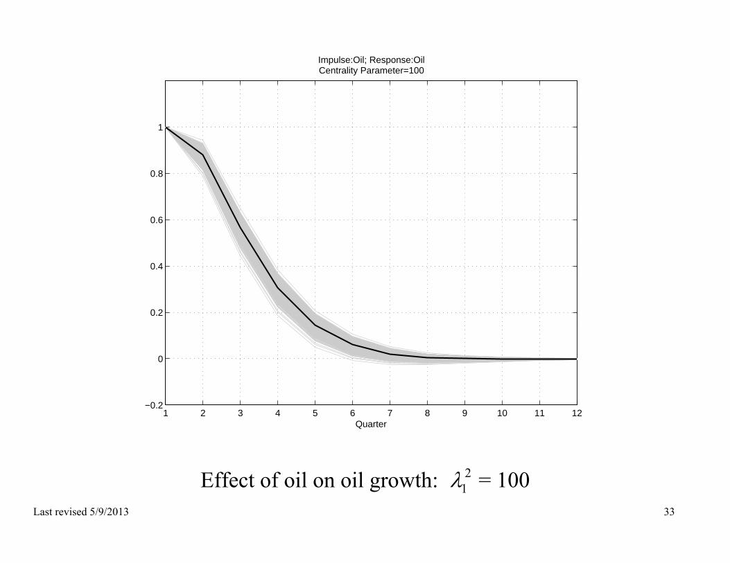
Effect of oil on oil growth: 21 = 100
1 2 3 4 5 6 7 8 9 10 11 12−0.2
0
0.2
0.4
0.6
0.8
1
Quarter
Impulse:Oil; Response:OilCentrality Parameter=100
Last revised 5/9/2013 34
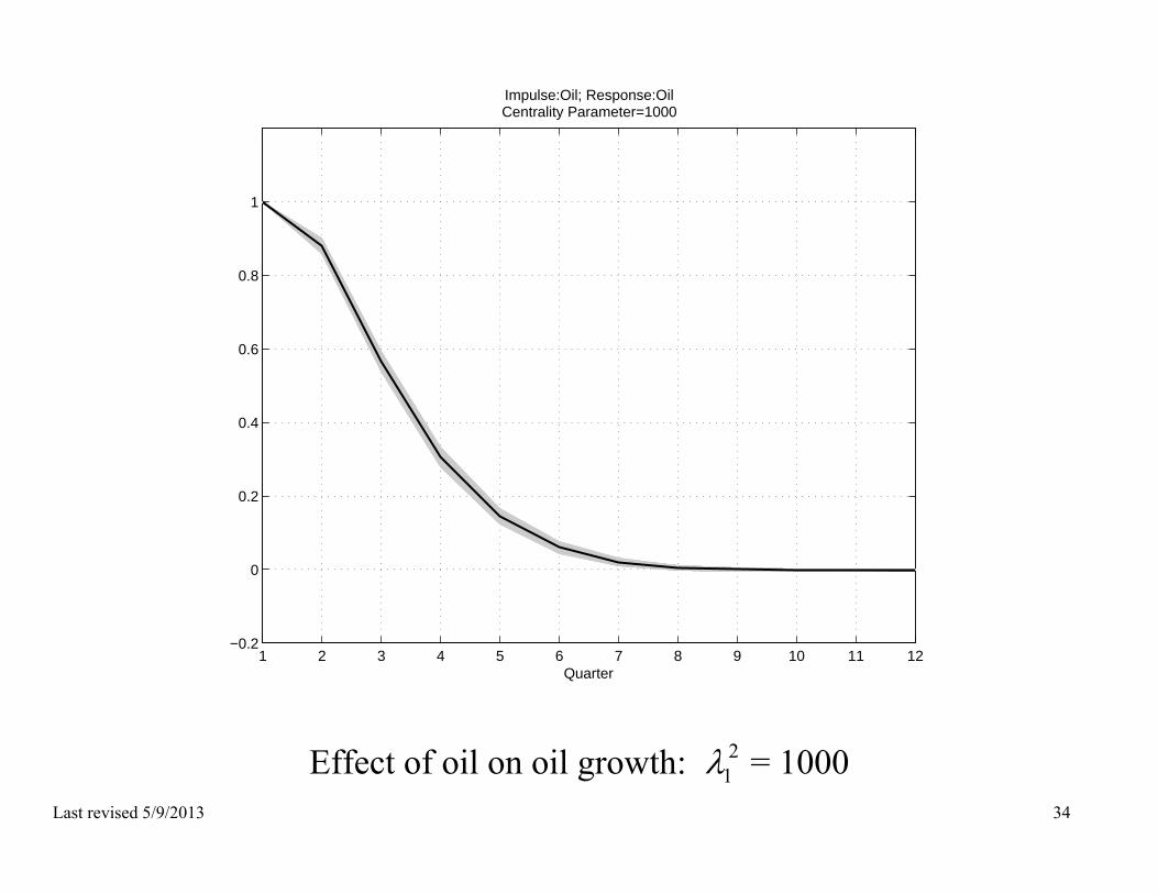
Effect of oil on oil growth: 21 = 1000
1 2 3 4 5 6 7 8 9 10 11 12−0.2
0
0.2
0.4
0.6
0.8
1
Quarter
Impulse:Oil; Response:OilCentrality Parameter=1000
Last revised 5/9/2013 35
Effect of oil on GDP growth: 21 = 100
1 2 3 4 5 6 7 8 9 10 11 12−1
−0.8
−0.6
−0.4
−0.2
0
0.2
Quarter
Impulse:Oil; Response:OutputCentrality Parameter=100
Last revised 5/9/2013 36
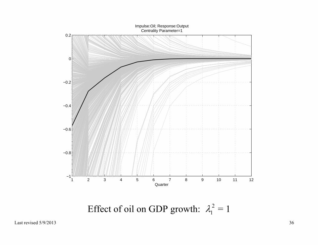
Effect of oil on GDP growth: 21 = 1
1 2 3 4 5 6 7 8 9 10 11 12−1
−0.8
−0.6
−0.4
−0.2
0
0.2
Quarter
Impulse:Oil; Response:OutputCentrality Parameter=1
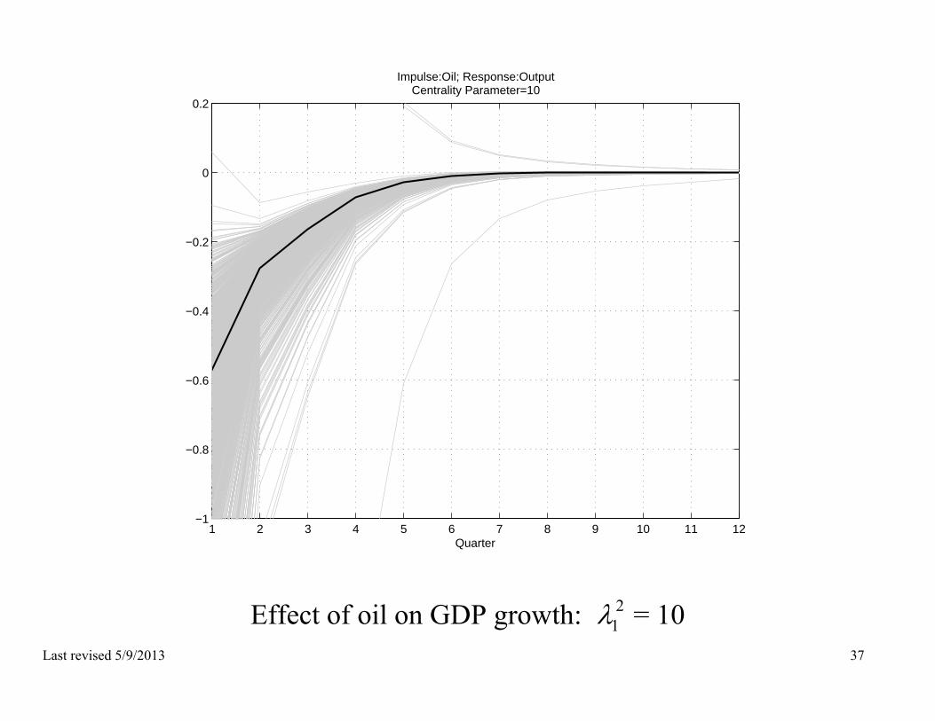
Last revised 5/9/2013 37
Effect of oil on GDP growth: 21 = 10
1 2 3 4 5 6 7 8 9 10 11 12−1
−0.8
−0.6
−0.4
−0.2
0
0.2
Quarter
Impulse:Oil; Response:OutputCentrality Parameter=10
Last revised 5/9/2013 38
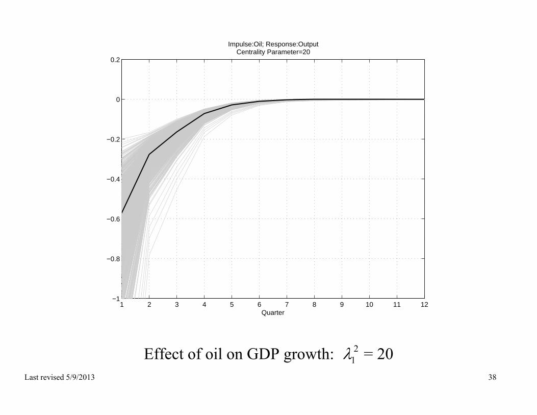
Effect of oil on GDP growth: 21 = 20
1 2 3 4 5 6 7 8 9 10 11 12−1
−0.8
−0.6
−0.4
−0.2
0
0.2
Quarter
Impulse:Oil; Response:OutputCentrality Parameter=20

Last revised 5/9/2013 39
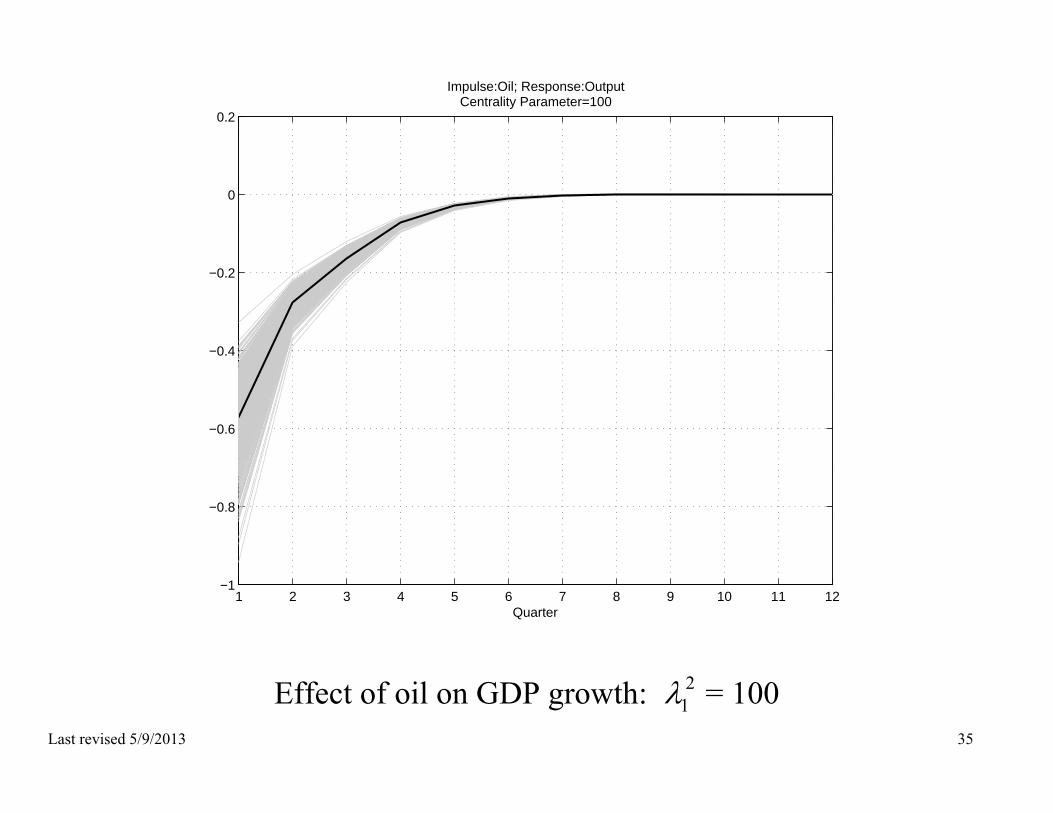
Effect of oil on GDP growth: 21 = 100
1 2 3 4 5 6 7 8 9 10 11 12−1
−0.8
−0.6
−0.4
−0.2
0
0.2
Quarter
Impulse:Oil; Response:OutputCentrality Parameter=100
Last revised 5/9/2013 40
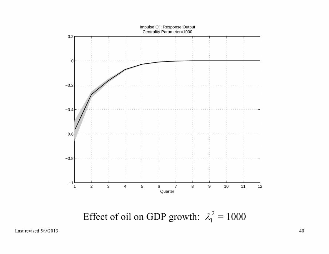
Effect of oil on GDP growth: 21 = 1000
1 2 3 4 5 6 7 8 9 10 11 12−1
−0.8
−0.6
−0.4
−0.2
0
0.2
Quarter
Impulse:Oil; Response:OutputCentrality Parameter=1000
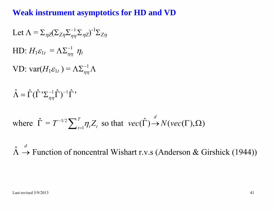
Last revised 5/9/2013 41
Weak instrument asymptotics for HD and VD Let = Z(Z
1 Z)-1Z
HD: H11t = 1 t
VD: var(H11t ) = 1
1 1ˆ ˆ ˆ ˆ ˆ( ' ) '
where = 1/21
Tt tt
T Z so that ˆ( ) ( ( ), )
dvec N vec
d Function of noncentral Wishart r.v.s (Anderson & Girshick (1944))
Last revised 5/9/2013 42
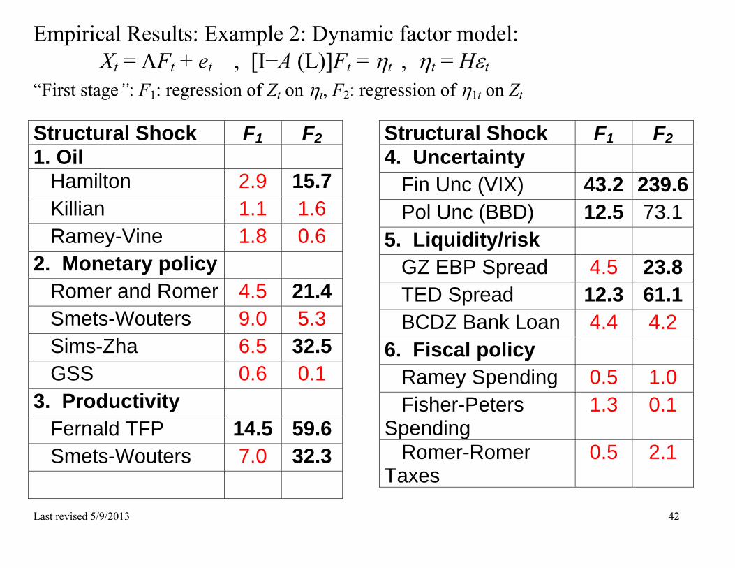
Empirical Results: Example 2: Dynamic factor model: Xt = Ft + et , [I−A (L)]Ft = t , t = Ht
“First stage”: F1: regression of Zt on t, F2: regression of 1t on Zt Structural Shock F1 F21. Oil Hamilton 2.9 15.7 Killian 1.1 1.6 Ramey-Vine 1.8 0.6 2. Monetary policy Romer and Romer 4.5 21.4 Smets-Wouters 9.0 5.3 Sims-Zha 6.5 32.5 GSS 0.6 0.1 3. Productivity Fernald TFP 14.5 59.6 Smets-Wouters 7.0 32.3
Structural Shock F1 F24. Uncertainty Fin Unc (VIX) 43.2 239.6 Pol Unc (BBD) 12.5 73.15. Liquidity/risk GZ EBP Spread 4.5 23.8 TED Spread 12.3 61.1 BCDZ Bank Loan 4.4 4.2 6. Fiscal policy Ramey Spending 0.5 1.0 Fisher-Peters Spending
1.3 0.1
Romer-Romer Taxes
0.5 2.1

Last revised 5/7/2013 43
Correlations among selected structural shocks
OilKilian oil – Kilian (2009) MRR monetary policy – Romer and Romer (2004) MSZ monetary policy – Sims-Zha (2006) PF productivity – Fernald (2009) UB Uncertainty – VIX/Bloom (2009) UBBD uncertainty (policy) – Baker, Bloom, and Davis (2012) LGZ liquidity/risk – Gilchrist-Zakrajšek (2011) excess bond premium LBCDZ liquidity/risk – BCDZ (2011) SLOOS shock FR fiscal policy – Ramey (2011) federal spending FRR fiscal policy – Romer-Romer (2010) federal tax
OK MRR MSZ PF UB UBBD SGZ BBCDZ FR FRROK 1.00 MRR 0.65 1.00 MSZ 0.35 0.93 1.00 PF 0.30 0.20 0.06 1.00 UB -0.37 -0.39 -0.29 0.19 1.00 UBBD 0.11 -0.17 -0.22 -0.06 0.78 1.00 LGZ -0.42 -0.41 -0.24 0.07 0.92 0.66 1.00 LBCDZ 0.22 0.56 0.55 -0.09 -0.69 -0.54 -0.73 1.00
FR -0.64 -0.84 -0.72 -0.17 0.26 -0.08 0.40 -0.13 1.00 FRR 0.15 0.77 0.88 0.18 0.01 -0.10 0.02 0.19 -0.45 1.00

Last revised 5/7/2013 44
Weak instrument asymptotics for cross-shock correlation Correlation between two identified shocks: Let Z1t and Z2t be scalar instruments that identify 1t and 2t:
Cor(1t2t) = 12 = 1 2
1 1 2 2
1
1 1
Z Z
Z Z Z Z
1/2
1 1 11 1211/2
2 21 222 2
ˆ,
ˆd
t t
t t
T ZN
T Z
r12 = 1 2
1 1 2 2
1 11 2
1 1 1 11 1 2 2
ˆ ˆ ˆ ˆ
ˆ ˆ ˆ ˆ ˆ ˆ ˆ ˆZ Z
Z Z Z Z
under null, 1ꞌ2 = 0
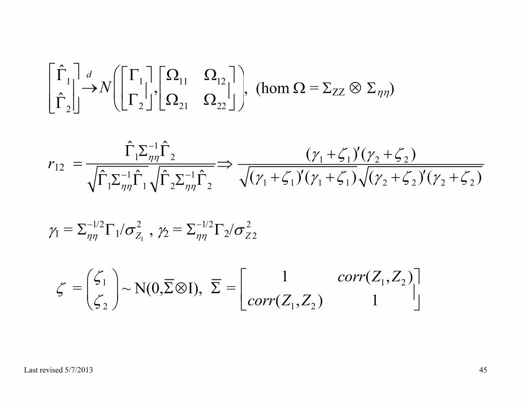
Last revised 5/7/2013 45
1 1 11 12
2 21 222
ˆ,
ˆd
N
, (hom = ZZ )
r12 1
1 2
1 11 1 2 2
ˆ ˆ
ˆ ˆ ˆ ˆ
1 1 2 2
1 1 1 1 2 2 2 2
( ) ( )( ) ( ) ( ) ( )
1 = 1/2
1/ 1
2Z , 2 = 1/2
2/ 2
2Z
= 1
2
~ N(0,I), = 1 2
1 2
1 ( , )( , ) 1
corr Z Zcorr Z Z

Last revised 5/7/2013 46
Weak instrument asymptotics for cross-shock correlation, ctd.
r12 1 1 2 2
1 1 1 1 2 2 2 2
( ) ( )( ) ( ) ( ) ( )
Comments 1. Nonstandard distribution – function of noncentral Wishart rvs 2. Normal under null as 11 and 22
3. Strong instruments under alternative: r12 p 1 2
1 1 2 2
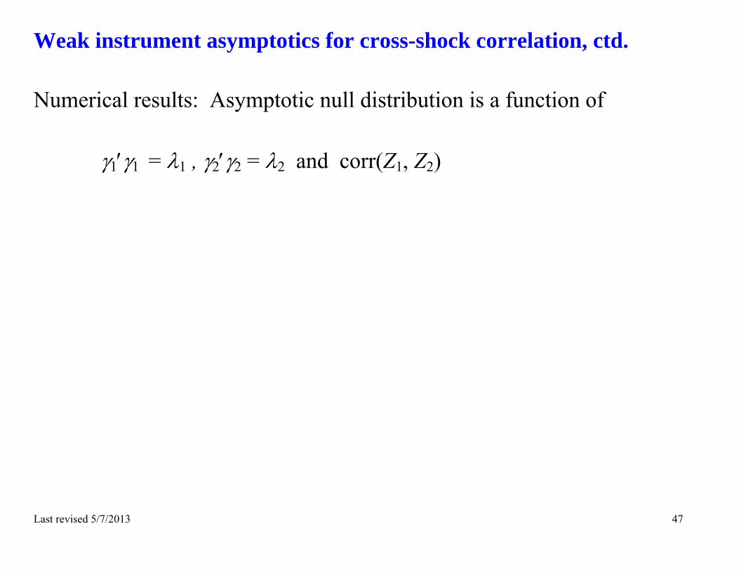
Last revised 5/7/2013 47
Weak instrument asymptotics for cross-shock correlation, ctd. Numerical results: Asymptotic null distribution is a function of
11 = 1 , 22 = 2 and corr(Z1, Z2)
Last revised 5/7/2013 48
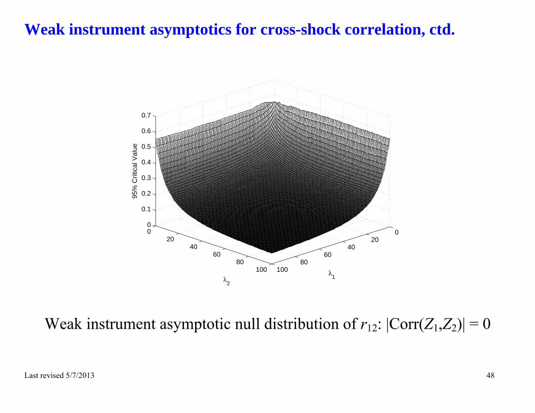
Weak instrument asymptotics for cross-shock correlation, ctd.
Weak instrument asymptotic null distribution of r12: |Corr(Z1,Z2)| = 0
020
4060
80100
020
4060
80100
0
0.1
0.2
0.3
0.4
0.5
0.6
0.7
λ1λ
2
95%
Crit
ical
Val
ue

Last revised 5/7/2013 49
Weak instrument asymptotics for cross-shock correlation, ctd.
Weak instrument asymptotic null distribution of r12: |Corr(Z1,Z2)| = 0.4
020
4060
80100
020
4060
80100
0
0.1
0.2
0.3
0.4
0.5
0.6
0.7
0.8
λ1λ
2
95%
Crit
ical
Val
ue

Last revised 5/7/2013 50
Weak instrument asymptotics for cross-shock correlation, ctd.
Weak instrument asymptotic null distribution of r12: |Corr(Z1,Z2)| = 0.8
020
4060
80100
020
4060
80100
0
0.2
0.4
0.6
0.8
1
λ1λ
2
95%
Crit
ical
Val
ue
Last revised 5/7/2013 51
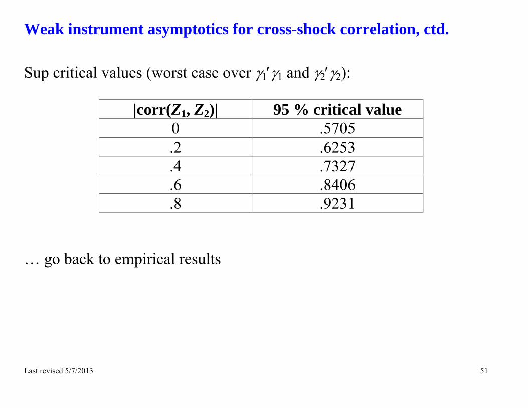
Weak instrument asymptotics for cross-shock correlation, ctd.
Sup critical values (worst case over 11 and 22):
|corr(Z1, Z2)| 95 % critical value 0 .5705 .2 .6253 .4 .7327 .6 .8406 .8 .9231
… go back to empirical results

Last revised 5/7/2013 52
Weak instrument asymptotics for reduced rank restriction Let Z1t and Z2t be scalar instruments that identify 1t: Z = H1ꞌ has rank 1
1/21 1 11 121
1/22 21 222 2
ˆ,
ˆd
t t
t t
T ZN
T Z
where 2 = b1
Last revised 5/7/2013 53
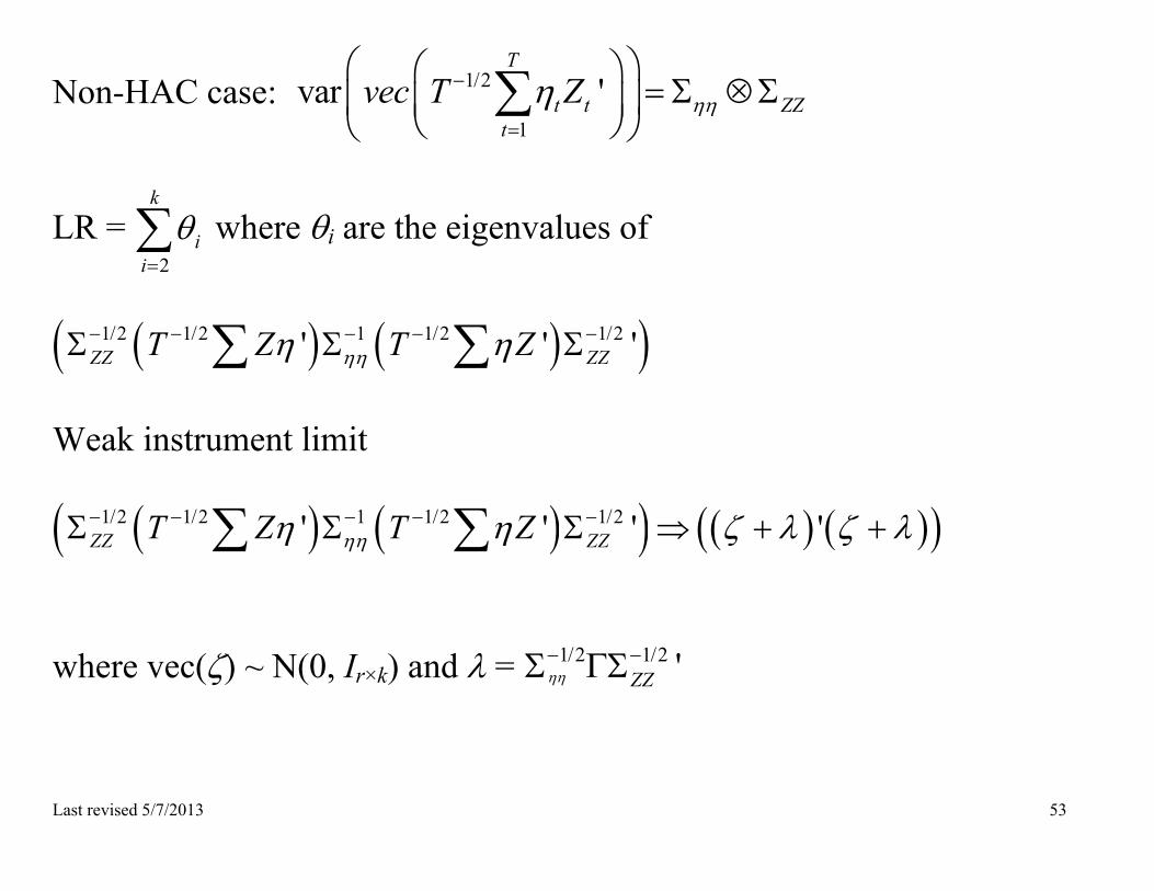
Non-HAC case: 1/2
1var '
T
t t ZZt
vec T Z
LR = 2
k
ii
where i are the eigenvalues of
1/2 1/2 1 1/2 1/2' ' 'ZZ ZZT Z T Z
Weak instrument limit
1/2 1/2 1 1/2 1/2' ' ' 'ZZ ZZT Z T Z where vec() ~ N(0, Ir×k) and = 1/2 1/2 'ZZ

Last revised 5/7/2013 54
1/2 1/2 1 1/2 1/2' ' ' 'ZZ ZZT Z T Z Limiting distribution of OID test depends on vec()’vec(). vec()’vec() large, OID 2
1
d
n vec()’vec().= 0, OID = sum of n-1 smallest eigenvalues of ’. n = 3
(vec()’vec())1/2 95% CV 100 7.8 (= 2
3 cv) 50 7.8 10 7.8 1 6.0 0 4.2
Last revised 5/7/2013 55
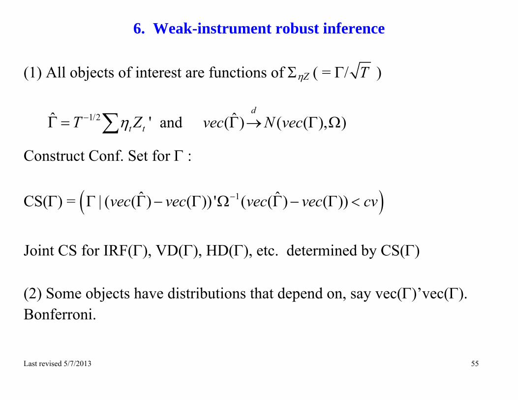
6. Weak-instrument robust inference
(1) All objects of interest are functions of Z ( = / T )
1/2ˆ 't tT Z and ˆ( ) ( ( ), )d
vec N vec
Construct Conf. Set for : CS() = 1ˆ ˆ| ( ( ) ( )) ' ( ( ) ( ))vec vec vec vec cv
Joint CS for IRF(), VD(), HD(), etc. determined by CS() (2) Some objects have distributions that depend on, say vec()’vec(). Bonferroni.
Last revised 5/7/2013 56
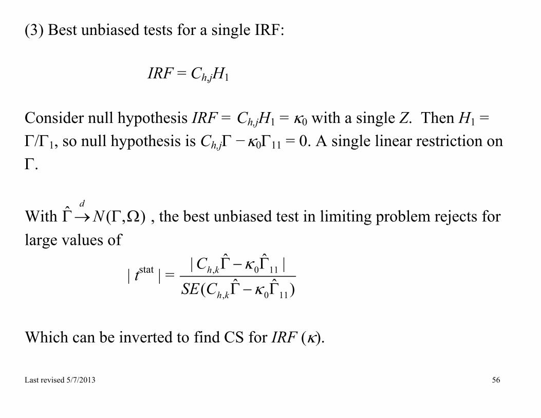
(3) Best unbiased tests for a single IRF:
IRF = Ch,jH1
Consider null hypothesis IRF = Ch,jH1 = 0 with a single Z. Then H1 = /1, so null hypothesis is Ch,j −011 = 0. A single linear restriction on .
With ˆ ( , )d
N , the best unbiased test in limiting problem rejects for large values of
| tstat | = , 0 11
, 0 11
ˆ ˆ| |ˆ ˆ( )
h k
h k
CSE C
Which can be inverted to find CS for IRF ().
Last revised 5/7/2013 57
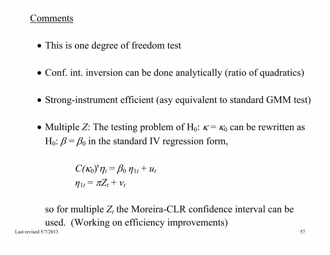
Comments This is one degree of freedom test
Conf. int. inversion can be done analytically (ratio of quadratics)
Strong-instrument efficient (asy equivalent to standard GMM test)
Multiple Z: The testing problem of H0: = 0 can be rewritten as
H0: = 0 in the standard IV regression form,
C(0)ꞌt = 0 η1t + ut η1t = Zt + vt
so for multiple Zt the Moreira-CLR confidence interval can be used. (Working on efficiency improvements)

Last revised 5/7/2013 58
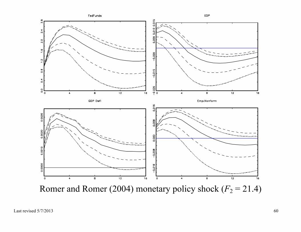
Examples: IRFs: strong-IV (dashed) and weak-IV robust (solid) pointwise bands
Hamilton (1996, 2003) oil shock (F2 = 15.7)

Last revised 5/7/2013 59
Kilian (2008) oil shock (F2 = 1.6)
Last revised 5/7/2013 60
Romer and Romer (2004) monetary policy shock (F2 = 21.4)

Last revised 5/7/2013 61
Conclusions Work to do includes Inference on correlations and on tests of overID restrictions in general Efficient inference for k > 1 (beyond Moreira-CLR confidence sets) –
exploit equivariance restriction to left-rotations (respecify SVAR in terms of linear combination of Y’s – this should reduce the dimension of the sufficient statistics in the limit experiment)
Inference in systems imposing uncorrelated shocks Formally taking into account “higher order” (Op(T—1/2)) sampling
uncertainty of reduced-form VAR parameters HAC (non-Kronecker) case: (a) robustify; (b) efficient inference?


![INDEX [impa.br]...Pedro C. Ferreira Fundação Getulio Vargas, FGV/EPGE Paul J. Gertler University of California, Berkeley Maitreesh Ghatak London School of Economics Delfim Gomes-Neto](https://static.fdocuments.us/doc/165x107/60b5bfc0d0cd234e45340ec8/index-impabr-pedro-c-ferreira-fundao-getulio-vargas-fgvepge-paul-j.jpg)