Developing Country Borrowing and Domestic Wealth

by

Mark Certler

and

Kenneth Rogoff

University of Wisconsin

February 1989

Revised June 1989

ABSTRACT

Across developing countries, capital market inefficiencies tend todecrease and external borrowing tends to sharply increase as national wealthrises. We construct a simple model of intertetnporal trade under asymmetricinformation which provides a coherent explanation of both these phenomenon,without appealing to imperfect capital mobility. The model can be applied toa number of policy issues in LDC lending, including the debt overhang problem,and the impact of government guarantees of private debt to foreign creditors.In the two—country general equilibrium version of the model, an increase inwealth in the rich country can induce a decline in investment in the poorcountry via a “siphoning effect”. Finally, we present some new empiricalevidence regarding the link between LDC borrowing and per capita income.

We are grateful to the National Science Foundation, the Sloan Foundation,and the Bradley Foundation for financial support, and to seminar participantsat the International Finance Division of the Federal Reserve Board for helpfulcomments on an earlier draft.

I. Introduction

This paper develops a model in which the efficiency of domestic capital

markets influences the pattern of international capital flows. Our analysis

is motivated by three general considerations: First, among developing

countries, external debt per capita tends to rise sharply with per capita GNP.

Second, capital markets operate less efficiently in poorer countries, as

Goldsmith (1969), HcKinnon (1973) and others have documented.1 One

manifestation of this phenomenon is that spreads between loan and deposit

rates tend to be higher in LDCs. Third, world capital markets are becoming

increasingly integrated so that, for example, covered interest differentials

are now fairly small across a broad range of countries. There are a variety

of theoretical models consistent with any one of these facts; our aim is to

present the simplest framework consistent with all three.

Our starting point is to modify the standard frictionless model of

interteinporal trade between countries by introducing informational asymmetries

between borrowers and lenders.2 At the micro level, these informational

frictions introduce a wedge between the costs of internal (to a finn) and

external finance. The size of the wedge is endogenously determined and

depends inversely on the net asset position of the individual borrower. At

the macro level, there emerges (ceteris paribus) a negative correlation

between the net wealth of a country and the spread between the domestic loan

1For an extensive recent discussion of capital market inefficiencies in

developing countries see World Bank 1989.

2 Our analysis draws on recent developments in the closed-economy literature

on interactions between the real and financial sectors; see Gertler (1988) fora survey. To abstract from sovereign risk, we assume that there is asupranational legal authority, capable of enforcing contracts across borders.Hence our analysis is really as much a model of capital flows betweenManhattan and the Bronx as between Japan and India.

1

rate and deposit rates. A corresponding result is that differences in

marginal products of capital can persist across countries even in a world with

perfectly integrated capital markets where riskless rates are equalized. We

show that these results can help explain the strong positive correlation

between country wealth and external borrowing among LDCs.

Section II presents a small—country model where investment finance is

constrained by a moral hazard problem. This stripped—down version of the

model is sufficient to illustrate our main results concerning developing—

country borrowing and the efficiency of developing—country capital markets.

In section III we extend the model to consider a nwaber of applications

involving private and public external borrowing by LUCs. These applications

include (a) the impact of foreign indebtedness on domestic investment, (b) the

effect of having the government guarantee private debt to foreign lenders, (c)

the indexation of foreign debts, Cd) explaining cross-country correlations

between domestic wealth and external debt.

Whereas the main applications we have in mind involve developing

countries, the analysis is also capable of providing insights into how

financial factors may influence capital flows between developed countries.3

Section IV provides a two—country general equilibrium version of the model,

which yields an interesting new perspective on the classic transfer problem:

Here, the cost to a country of having to transfer wealth is exacerbated by

information—induced inefficiencies. In general, increased wealth in one

country can improve the efficiency of its capital markets and thereby “siphon”

Kletzer and Bardhan (1987) discuss how differences in domestic financialmarket efficiency can influence patterns of trade. Our model differs in thatthe degree of the inefficiency is an endogenous product of the country’s stateof development, as summarized by its per capita wealth. Also, the structureof financial contracts is endogenous here.

2

investment funds from the other country.

Finally, in section V we present some empirical evidence aimed at

verifying the positive link between external borrowing and country wealth.

Using data from 1980 for a cross—section of seventy developing countries, we

show that for each percentage point increase in per capital income, per capita

external debt to private creditors tends to rise significantly more than one

percent. Moreover, this relation between external debt and national income

tends to hold across countries within the same region (Africa, Asia, and Latin

America). In the conclusions, we explain why our theory is likely to be at

least part of the explanation for this interesting fact.

II. A Small—Country Model with Agency Costs of Investment

Our goal throughout is to provide the simplest possible model capable of

illustrating our main points. Before turning to the two—country case, we

first develop and analyze a small—country framework. We consider an open

economy inhabited by a large number of identical individuals; the economy is

small in the sense that It cannot affect the world interest rate. There are

two periods and one good. The representative individual is risk neutral and

cares only about consuming in period two:

U(c) = c, (1)

where c is her second-period consumption.

Entering period one, each person is endowed with W units of the

consumption good.4 There exist two ways to convert this endowment into final

period consumption. The first option is to lend abroad at the (gross) world

4Later, we will amend the concept of wealth to include any collateralizablefuture income or illiquid assets.

3

riskless interest rate r; the alternative is to invest in a risky technology.

In particular, each person in the country has a project. All projects are

identical ex ante, and yield ex post returns as follows: k units invested in

period one yield e units of second—period output with probability ir(k), and

zero units with probability 1 — tr(k). That is,

( U with probability w(k)~ (2)

1% 0 “ “ 1 — 71(k)

where y is second—period output. The function id) is increasing, strictly

concave and twice continuously differentiable, with ~dO) = 0, n(w) = I, and

r/o C g’(O) < Thus, investment raises the probability that the

individual’s project will yield a high level of output, and the marginal

expected return to investment is diminishing.6 We assume that output

realizations are independent across the projects of different individuals.

If an individual wants to invest more than her endowment in her project,

then she must raise funds from the world capital market; that is,

W÷b~k (3)

where 1, is the amount she borrows. In return for this amount, she issues a

state—contingent security which pays ~ in the event the project yields the

good outcome, and in the event of the bad outcome. The security must offer

(0) > rIO is needed to guarantee that it is optimal to invest under perfect

information. It is not essential that n’ (0) be finite, but introducing thisrestriction makes the exposition a bit simpler.

6lt is easy to generalize the results to a technology with a large set ofpossible output realizations. We choose the two—point distribution for easeof exposition.

4

7

lenders the market rate of return r, so that

+ [1 — ir(k)]Z” rb (4)

The left—hand side of (4) is the expected payment to lenders.

The individual’s expected second period consumption is given by

E{c} = ir(k)[6 — Z9] — (1 — it(k)IZ1’ + nw + b — kI (5)

where the last term is the individual’s return from risk—free investments

abroad, and the first two terms represent the expected net return on her

project.

The information structure is as follows: Lenders may observe a borrower’s

initial wealth and the total amount she borrows. What the borrower does with

the funds, however, is her private knowledge. In particular, she may secretly

lend abroad rather than invest in her project. Whereas investment is

unobservable, lenders can freely observe realized output. The production

function u(S) is common knowledge.

If there were no information asymmetries, the individual would invest to

the point where the expected marginal project return equals the world interest

rate. Let k denote this first—best level of investment; thus

it’ (k’)o = r (6)

Under asymmetric information, however, it. is not generally possible to

implement the first best allocation because the borrower’ s choice of

investment k is not verifiable.8 Contracts can be conditioned only on

71t is not necessary to assume that lenders are risk neutral, but only thatidiosyncratic project risk be diversifiable in world capital markets.

8The incentive problem emerging here is classified as moral hazard because theinformational asymmetry arises after contracting. See Dixit (1987) for an

5

realized output y, and not on k. Given any output-contingent payoffs (2

g2

b)

specified by the contract, the borrower will pick k to maximize her expected

consumption, given by (5). Thus she will equate her expected marginal gain

from investing with her opportunity cost of (secretly) holding assets abroad9

— (Z~ — = r (7)

9 bSo long as 2 differs from Z , k will differ from its first—best optimum

10value k , given by (6). The problem is that the borrower’s marginal benefit

from investing depends not only on the marginal gain in expected output, but

on the change in her expected obligation to lenders, as well. We will

subsequently refer to (7) as the “incentive constraint.”

b *If the borrower could promise lenders a fixed payment 2 = 2 = r(k — W)

then [by (7)] she would invest the first best amount k’. This is not

feasible, however, since the project yields nothing in the bad state. Since

the borrower’s consumption must be non—negative, an important constraint on

the form of the contract is

(3)

For the case where Si C k the optimal incentive compatible contract is

found by choosing z~, zb, b, and k to maximize (5) subject to (3), (4), (7)

application to international trade.9The analysis would be qualitatively similar if the borrower had the option ofsecretly consuming in period one instead of secretly lending abroad.10Note that the Miller—Modigliani theorem fails under asymmetric informationbecause the investment decision depends on the structure of contract payoffs.The idea that informational asymmetries can affect an individual firm’sInvestment strategies and financial structure originated with Jensen andHeckling (1976).

6

and (8). The solution is as follows11: The contract pays lenders zero in the

bad state, so that (8) is binding. (More generally, the contract always pays

lenders the maximum feasible amount in the bad state. ) This serves to

minimize the spread between2

g and2

b, thereby minimizing the difference

between the borrower’s decision rule for k [eq. (7)] and the socially

efficient rule [eq. (6)]. Similarly, equation (3) is binding; 14 + b = k.

Thus, in equilibrium, the borrower does not secretly lend abroad. Borrowing

more than is essential to finance k would raise the gap between and

Since (3) and (5) hold with equality for the information—constrained

case, one can use these equations to eliminate b and from (4) and (7). The

result is the following two equations, which determine k and

— = r, IC curve (9)

= r(k — W)/it(k) MR curve (10)

Equation (9) is the incentive constraint, and is drawn as the curve IC in

Figure 1. It is downward sloping. A rise in Z9 lowers the borrower’s

expected marginal gain from investing and therefore must be offset by a

decline in k. The curve intersects the vertical axis at a value of Z~which

lies between zero and & (recall that riD < z’(O) C oo). It intersects the

horizontal axis at since eq. (9) resembles eq. (6) when Z~equals zero.

Equation (10) is the constraint that lenders must receive the market rate of

return, and is labeled as the MR curve. It is upward sloping. 12 When k rises,

~See the Appendix for details.

12The slope of the MR curve equals [rin(k)](l — •(k)(1 — 14/k)]; where •(k) isthe ratio of the marginal product of capital to the average product, given

by it’ (k)/(u(k)/k). Since 0 C 0(k) < I and since 14 < k along the MR curve, theslope must be positive.

7

Figure 1

EQUILIBRIUM IN lfl SMALL COUNTRYCASE

a

IC MR

14 k

k

-.1.

borrowing goes up; this means must rise since 2~’ cannot adjust. The curve

intersects the horizontal axis at k equal to U. It lies above the horizontal

axis at k since k > 14.

Investment in the information—constrained case must be below its first

0 *best value R . The result that k < k follows immediately from a comparison

of (6) and (9), as well as from inspection of Figure 1. If k is below k,

then ex post per capita output, Ou(k), must lie below its first best value,

13eiz(k ). An implication is that both per capita investment and per capita

output will depend on per capita wealth. A rise in 14 shifts the MR curve

downward in Figure 1 and leaves the IC curve unchanged, thereby raising k and

lowering Additional wealth increases the amount of internal funds

available to the borrower; so for a given level of investment, Z~declines,

mitigating the incentive problem. Investment rises, in accordance with

eq.(9), thus raising output as well.

Note that the spread between the marginal product of capital and the

world riskless interest rate will vary across countries, and in particular,

will be larger the poorer the country. Cross—country differences in marginal

products of capital may arise here even though the world capital market is

13Because the productivity risks are independent across investment projects,and because the number of projects is large, there is no aggregate risk.

14The result that increases in borrower net worth stimulate investment whenInformational problems are present is quite general; see Bernanke and Gertler(1989). For some empirical support, see Fazzari, Hubbard and Petersen (1988).

15The effect of a change in 14 on Ic is given by

= ir’(k)29/[(,z”(k)/u’(k))r — ir’(k)291 >0

where ~ = r(k — W)/ii(k), so that > 0 and ZY < 0.

8

perfectly integrated (the riskless rate is the same everywhere).16 A

corresponding result is that the spread between the loan rate and the riskless

rate will be higher in poor countries. The loan (risky debt) rate is given by

r/it(k), which is decreasing in k and therefore decreasing In U.

Finally, consider how changes in the world interest rate influence

investment. As r goes up, the IC curve shifts to the left. The borrower’s

opportunity cost of investing rises, so for any given value of Z9, k must

decline. The MR curve moves inward as well. Some combination of a rise in

2g and a fall in k is necessary for lenders to continue to receive a

competitive return. The interest—elasticity of investment in the information—

constrained case may or may not be greater than in the full information case.

It is greater if dZ~/dr > 0. This will likely be the case if the initial

amount borrowed, k — 14, is large or if the production function is sufficiently

concave so that the decline in k is not enough to offset the higher rate of

interest. 17

III. Applications to Private and Public External Borrowing by LIEs

The model developed here can readily be extended to consider a number of

issues involving developing—country borrowing:

APPLICATION 1: Debt Overhang

16Thus our model is completely consistent with Frankel and MacArthur’ s (1988)finding that covered interest differentials are relatively small for manyLDCs.

17The adjustment of Ic in response to a change in r is given by

= 11 + ix’ (k)Z9)/[(g”(k)/iz’ (kflr — it’ (k)Z”) < 0dr 1 2

where 2~(~,1) = r(k — W)/u(k), so that Z~> 0 and < 0.

9

Suppose the government has a debt outstanding to foreign lenders of rD

per capita, payable at the end of the second period. The government finances

the debt by taxing its citizens in period 2. Let t9 denote the tax on

successful entrepreneurs, and denote the tax on unsuccessful entrepreneurs;

bnote that r must be zero since unsuccessful entrepreneurs have no resources.

The government budget constraint is thus

rID = ~ (11)

Under perfect information, the introduction of the debt tax has no

bearing on an entrepreneur’s investment decision, which is still governed by

eq. (6). The debt tax is effectively a lump—sum tax on entrepreneurial rents.

Under asymmetric information, however, the tax leads to a decline in

investment because of its impact on entrepreneurial wealth.

The existence of the debt tax modifies the entrepreneur’s problem as

follows: Eqs. (1) — (4) remain unchanged. In eqs.(5), (7) (8) and (9), Z’~

and are replaced by ~ + ~ and + respectively; the entrepreneur’s

state—contingent obligations now include payments to the government as well

as to private lenders. Eq. (10), however, remains as before because the

introduction of taxes does not affect the restriction that lenders must

receive a competitive return. Making use of the government’s budget constraint

(12), the IC and MR curves can be written

— ~ + ~~)] = r IC’ curve (9’)

+ x’~) = r(k —14 + D)/ir(k) JIB’ curve (10’)

where = rD/it(k). In analogy with eqs. (9) and (10), one can think of eqs.

(9’) and (10’) as determining Z’ + ~ and k as a function of W — D. Thus the

10

impact on investment of a rise in governmentdebt to foreigners is the same as

the effect of a decline in U. Since the debt tax is indexed to income, it

reduces each entrepreneur’s incentive to invest. Note that this distortion

ultimately arises from the information structure and not from ad hoc

restrictions on the kinds of taxes the government can use.

APPLICATION 2: Government-Guaranteed Private Debt

In many LDCs, a considerable proportion of private foreign debt is

government guaranteed. What effect does this have on investment? Suppose

that the government guarantees a firm’s creditors a payment of in the event

of an unsuccessful outcome, and charges successful firms a tax of t9

. In this

case, the government budget constraint is given by

+ [1 — ir(k))o~ = 0 (12)

In eq. (4), the condition that lenders earn a competitive rate of return,

is replaced by z1)+ ~.t3 In eqs. (5) and ~ 2g is replaced by 2g +

reflecting that successful entrepreneurs are taxed to finance the loan

guarantees.

By employing the government budget constraint (12), it is easy to show

that the loan guarantee program has no impact on investment. The guarantee of

a payment in the bad states reduces the amount entrepreneurs must pay in the

good states, Z9. This lowers the spread between the entrepreneur’s payoffs to

lenders in different states and thus, other things equal, tends to mitigate

the incentive problem. However, this positive effect is completely offset by

the tax successful entrepreneurs must pay. Due to the government budget

constraint, ~ + t9 adjusts to equal what z9 would have been in the absence of

the loan guaranteeprogram.

The key to this neutrality result is that the government loan guarantee

11

program involves no redistribution. The guaranteeprogram, which benefits the

entrepreneurial sector, is completely financed by it. Obviously, if the

program is partly financed by other citizens, it will stimulate investment.

However, what is critical is the transfer of wealth across sectors and not the

vehicle of a loan guarantee program.

APPLICATION 3: Wealth Shocks and Irjdexatlon

We now further examine the impact of shocks to the country’s wealth.

First, it useful to broaden the concept of wealth to include not just current

liquid assets 14, but also any collateralizable illiquid assets such as proven

oil reserves or the secureportion of future earnings.18 Changesin the value

of illiquid assets are likely to account for a considerable portion of the

volatility in a country’s wealth. Let V denote the period—two payoff to each

entrepreneur from collateralizable illiquid assets.19 The entrepreneur’s

formal problem remains as before, except that V is added to the right—hand

side of eq. (5) [the eq. for expected second—period consumption), and the

limited liability constraint, eq. (8), is relaxed to be ~ V. It is easy to

show that the determination of k is the same as before except that the

relevant measure of wealth is now 14 + V/r.

Randomness in wealth can lower welfare even though all citizens are risk

neutral. To see this, first note that because of the role of wealth in

reducing agency costs, the shadow value of a unit of wealth may exceed r.

Differentiating the entrepreneur’s objective function (5) at the optimum

18 This generalized concept of borrower wealth arises in a dynamic setting.

See Gertler (1988), who studies a closed—economy with repeated production andasymmetric information where entrepreneurs enter long-term financial contractswith lenders.

may be random so long as the distribution is common knowledge.

12

implies:

OE{c}/6(W + V/r) = (Sn’(k) — r)[ak/8(W + V/r)) + r t r (13)

where the inequality holds strictly when the incentive constraint binds (where

U + V/r C k). One can show that given a very weak restriction on the third

derivative of the production function it, the marginal gain in expected

consumptiondiminishes as wealth rises; i.e. 82E{é}/[8(W + V/r)12 c o.2° Thus

expected consumption is strictly concave in wealth (when the incentive

constraint is binding).

Consider then, the problem of a country whose collateralizable “illiquid”

wealth consists of proven oil reserves. From application 1, we know that it

does not matter whether each entrepreneur owns a share of the oil directly, or

whether the oil revenue is rebated to citizens by the government. Suppose

that oil production is exogenous and that a manufactured good is produced in

the entrepreneurial sector; this is the only good consumed locally. (All of

the country’s oil is exported.) A shock to the world price of oil (vis—â—vis

the traded good) can then be interpreted as a shift in V. Note that in the

presence of asymmetric information, fluctuations in the world price of oil

will induce fluctuations in domestic manufacturing investment via their impact

on entrepreneurial wealth. The investment fluctuations will be asymmetric,

since a unit decline in wealth leads to a bigger absolute change in k than

does a unit increase.21 The effect of oil price shocks on GNP is similarly

asymmetric.

20 A sufficient condition to assure that 32E{c)/[3(W + V/rH2< 0 is that

2[ii”(k)n(k)/[n (k)] is increasing in k. (This condition guarantees that

d2k/[d(W + V/r)]2 c 0.)21 This is true because k is strictly increasing and concave in 14 + V/r.

13

Thus, even apart from the usual risk aversion arguments, a developing

country may want to Index its repaymentsto the price of its

(collateralizable) commodity exports. By smoothing the impact of commodity

price shocks on wealth, the country can reduce the impact of credit market

inefficiencies on investment in other sectors of the economy.

To the extent that shocks to 14 reflect the impact of saving, then a

correlation between saving and investment will emerge even though the country

is small and capital markets are perfectly integrated. Thus the model

provides a somewhat different explanation of the Feldstein—}{orioka (1980)

puzzle. The usual explanations rely either on imperfect capital markets

(Feldstein and }-lorioka’s preferred rationale) or on particular patterns of

22technology shocks.

APPLICATION 4~ Patterns of External Borrowing Across LDCs

Our analysis suggests that there should exist a strong link between

external borrowing b (equal to k — U) and country wealth among the set of low

wealth countries. The exact effect of wealth on patterns of external

borrowing will depend on whether it is liquid assets, U, or illiquid assets,

V, which differ most across LDCs. Clearly, db/d(V/r) = dk/d(V/r) > 0;

external borrowing rises with a rise in V/r since investment rises and the

supply of internal (liquid) funds is unchanged. The net effect of a change in

liquid assets U on b depends on the sensitivity of k to changes in U.

Differentiating eqs. (9) and (10) implies

= - = - ~(k)(1-W/k) - _______ - 1 (14)it (k)

22 Obstfeld (1986) shows how a strong savings-investment correlation could

arise in a frictionless setting if technology shocks are dominant.

14

where

0 C 0(k) = n’(k)/[n(k)/kl C I

External borrowing will rise with U if a dollar increase in wealth induces

more than a dollar increase in investment. This will be the case if

diminishing returns set in slowly, i.e., if t”(k) is small relative to 7r’(k).

(Inspection of eq. (14) indicates that the magnitude of varies inversely

with the absolute value of n”(k)/w’(k).)

Since illiquid assets represent the lion’s share of wealth for most

countries, the overall correlation between wealth and external borrowing

across poor countries is likely to be positive.

IV. The Two-Country General Equilibrium Case

Thus far we have devoted our attention to the case of small developing

countries. Although the capital market imperfections characterized here are

likely to be most severe for poor countries, the model can also be applied to

analyze how financial factors may influence capital flows between large

developed economies. (An alternative interpretation of the two—country

analysis below involves having the developing countries as one group, and the

industrialized countries as the other.

Suppose there are two countries of equal population size, country B

(“rich”) and country P (“poor”). In each country, a percent of the

individuals are “entrepreneurs” and 1—a percent are “lenders.” All

individuals have the same utility function, given by equation (1). That is,

they are risk neutral and care only about second period consumption. Entering

the first period, all entrepreneurs in the poor country are endowed with U”

units of the good, and all lenders are endowed with14

PL units. Similarly,

entrepreneurs and lenders in the rich country are endowed with and

15

units, respectively. For the time being, the only restriction we need impose

is that it < it. (For now, we abstract from collateralizable illiquid

assets. )

Each entrepreneur owns and manages a risky investment project. The

project technology is the same across entrepreneurs and across countries, and

is given by equation (2) above. As before, if an entrepreneur wants to invest

more than her endowment she has to borrow, so that equation (3) still applies.

Lenders do not have projects; their only option is to lend to entrepreneurs. 23

The information structure is the same as in the small—country case.

Lenders observe a project’s realized output, but cannot observe the capital

input. They cannot directly see whether the entrepreneur is secretly lending

to other entrepreneurs. 24

If there were no information asymmetries, the following three equations

would characterize the world equilibrium:

p.n’(lc )O = r (15)

*ir’(k )e = r (16)

+ V) = aRt + It) + (l_a)(VL + ItL) (17)

where the P and B superscripts denote the countries, and the •‘s denote the

full—information equilibrium. The main difference from the small—country case

is, of course, that the world interest rate r is endogenous. It depends on

technology and the total world endowment. Since the technologies are the

23Without lenders, entrepreneurswould not be borrowers in the world generalequi libriuin.

24Note that entrepreneurs may secretly rechannel their investment funds eitherdirectly, or through a (zero—profit) intermediary.

16

same, k equals Ic . Under perfect information, the pattern of investments

is independent of the pattern of endowments.

Under asymmetric information, the following five equations characterize

the world equilibrium:

— = r (18)

— = r (19)

= nV - W”]/z(k”) (20)

29R = r(kR - Itl/~(kR) (21)

+ k’~) = a(W’~ + it) + (l—a)(V’~ + W’~’~) WV curve (22)

Equations (18) and (19) correspond to equation (9) for the small country

case, and equations (20) and (21) correspond to equation (10). Equation (22)

is the condition that the total demand for investment capital must equal the

world supply, and is drawn as the negatively—slopedWV curve in Figure 2.

Investment in the poor country is now less than in the rich country.

Combining equations (18) through (21) yields

r = p(k’3,W”)e = p(k’~,it)O pp curve (23)

where the function p(, .) is given by

it’ (k3)p(k~,W~)= , J = P,R (24)

1 + 7e(k~)[V— W~]/ir(k~)

As indicated in equation (23), p1 C 0 and p2 > 0. It follows immediately that

< k’~, since it < it. Because investment is distorted, world output is

lower than in the perfect information case. The world interest rate must also

be lower; this is easily demonstrated by comparing conditions (19) and (16),

17

Figure 2

EQUILIBRiUM IN TUE TWO COUNTRYCASE

WV

and noting that > and that2

g > 0. Thus lenders must be worse off

under asymmetric Information, Equation (23) is drawn as the positively—sloped

pp curve In Figure 2.

In general, the pattern of world investment depends on the agency costs

of lending in one country relative to the other, which in turn depends on the

net asset positions of entrepreneurs across countries.25 To illustrate this

point, suppose that the wealth of rich country entrepreneurs improves, but

that both total world endowment and the endowments of poor country

entrepreneurs remain unchanged. Consider, for example, a redistribution of

wealth in the rich country from lenders to entrepreneurs. This corresponds to

an upward rotation in the pp curve in Figure 2; the WV curve remains

unchanged. rises and k” falls. The decline in the agency costs of finance

in the rich country induces a ‘siphoning’ of investment funds from the poor

country.26 The Increased demand for funds by rich co~mtry entrepreneurs drives

up the world interest rate, drawing capital out of the poor country.

R P p.[Inspection of eq. (23) indIcates that ar/OW > 0 since k declines and 14 is

unchanged. I Entrepreneurs in the poor country lose rents as a result of the

capital flight. This loss of rents Is aggravated by the rise In the world

interest rate. Lenders in the poor country benefit from the rise in interest

rates but as long as the poor country is a net borrower, Its national income

must fall.

important difference between our model and earlier frameworks emphasizing

capital market frictions (e.g., Persson and Svenson (1989)) Is that theimperfections and the forms of the financial contracts are derivedendogenously. An Important exception Is Greenwood and Williamson (1989) whodevelop a monetary model of International business fluctuations underincomplete information. Another related paper is Samolyk (1988), who studiesthe transmission of regional disturbances in financial markets.

26See the appendix for an analytical derivation.

18

A fall In the wealth of poor country entrepreneurs similarly induces

siphoning of capital from the poor to the rich country. The reduced

efficiency of lending In the poor country causes funds to flow out to the

world capital market. In contrast to the previous case, the world interest

rate declines. [Inspection of eq. (23) Indicates that < 0 since 1c~~

increases while W’1 remains unchanged. I The shift of investment funds from the

high marginal product of capital poor country to the low marginal product of

capital rich country depresses the equilibrium interest rate.

Now consider a transfer of wealth from the poor country to the rich. In

particular, suppose that t units of wealth are taken from each citizen of the

poor country and are distributed evenly among the citizens of the rich

country. This transfer can also be graphed as an upward rotatiort of the pp

curve in flgure 2. However, for a given change in the pp curve shifts by

more than for our earlier example in which the transfer came from rich country

lenders. Both the increase in and the decline in induce to rise and

to fall. The net effect on the world Interest rate is ambiguous; greater

tends to move the interest rate up while less moves it down, as

discussed earlier. Uate that under perfect Information a similar transfer of

wealth would affect neither investment nor the interest rate [see eqs. (is) —

(17)1.

The wealth transfer naturally imposes a direct cost on the poor country.

But there may be Indirect costs as well. Holding constant the world interest

rate, entrepreneurs In the poor country lose additionally because their

project rents decline due to the reduction in investment. Thus, to the extent

that the movement In the world interest rate is not large, the indirect

effects always magnify the costs of the transfer. If the change in the

interest rate is large (owing to highly concave production functions) then the

19

exact effect on the poor country’s national income dependson whether it Is a

net debtor or creditor In the world capital market. However, if the poor

country is small, the movement in r Is negligible so that the capital market

problems always magnify the costs of wealth transfers.

This model accordingly produces a “transfer’4 problem in the sense that

the cost to a óountry of paying a foreign debt may exceed the face value of

the payments. Here the transfer problem relates to intertemporal trade rather

than contemporaneous trade, as In the classic debate between Keynes (1929) and

Ohlin (1929). It arises because the distribution of wealth affects the

allocation of investment, due to Information asymmetries. The more general

point is that any factor caus1ng a redistribution of wealth between coimtries

(e.g., due to exchange rate movements) will tend to make capital flow from the

losing to the winning country.

As another variation on this theme, consider a shock which increases the

Initial endowment of all Individuals in the rich country, thus Increasing the

total supply of investment funds available to the world capital market.

Under perfect information, capital investment would rise the same in each

country. But under asymmetric information, there will be a siphoning effect

since the wealth of rich country entrepreneursrises as well. Thus the

increase In Investment will be greater In the rich country, and It is even

conceivable that investment may decline in the poor country.

As discussed earlier, the relevant measure of a borrower’s wealth, W,

includes not only liquid assets, but any collateralizable expected future

profits as well (see Application 3). Thus good news about future business

conditions in the rich country can also induce the ‘siphoning’ effect

described above.

Finally, we consider a shock to world productivity, 0. By inspection of

20

of equation (23), we see that a world productivity shock has no effect on the

distribution of investment capital, since S factors out of both sides. As in

the full information case, the rise in 0 Increases per capita world output and

the world interest rate r

V. External Debt and GNP for Developing Countries

Perhaps the most direct evidence one could provide in support of our

model would be to show that acrossdeveloping countries, the marginal return

on Investment is higher the poorer the country, Although such an exercise is

clearly feasible, it is a very significant undertaking which involves

estimating production fwictlons across a broad range of developing countries.

However, there does exist some supporting evidence for a related prediction of

our model, which is that the spreads between the risk-free rate and the

risky—debt rate should be larger In poor countries.27 Some of these

differences may be due to differences in the tax treatment of banks and In

bank regulation across countries, but the kinds of financial market

imperfections considered here may also be important.

In this section we investigate another empirical implication of our

model, which Is that per capita external borrowing should be Increasing In per

capita wealth across developing countries. There are other models which

can also explain the evidence presented below. However, one factor In favor

of our general story 1s that it Is also consistent with the broad range of

27 See Goldsmith (1969), Hansen (1986) and Rocha (1986). Obviously,

differences in spreads across countries also depend on differences In the taxand regulatory treatment of banks. Spreads in Industrialized countries tendto be two to three percent. They are nominally the sante in non—inflationaryLDCs but are effectively much higher when the added transactions costs facingborrowers and depositors are taken Into account. In Inflationary LDCS spreadstypically exceed ten percent. See World Bank 1989.

st..

21

TA.aLE I

Measures of £txternal Borrowing Versus GYP: 1980

DOLLARS PER CA?ITA

External Debt TotalalP to Private Lenders External Debt

Ethiopia 107 3 21Uganda 131 16 56Nepal 142 0 15Bangladesh 144 3 45Chad 162 14 49Burma. 173. 9 45Malawi 190 51 136Burundi 222 5 40Rwanda 226 6 37Mali 231 8 102.Burkina Paso 234 9 54India 256 3 29Sfl Lanka 271 25 125Tanzania 276 46 138Pakistan 283 1.6 120Balti 289 7 60Sierra Leone 321 51aenin 331 69 120Cen. Aft. Rep. 343 30 82Sudan 358 78 268Somalia 361 13 191Madagascar 370 68 144Zaire 380 71 183Ghana 384 24 114Kenya 412 117 210Mauritania 412 122 511Togo 435 208 408Niger 472 111 163t1esotho 481 1.4 53Senegal 504 106 - 225Yemen A.R. 508 17 165IndonesIa 512 78 - 143Egypt 514 149 470Bolivia 516 263 482Liberia 591 131 383Zambia 617 226 558Honduras 648 201 400Thailand 686 124 178Philippines 729 284 360El Salvador 780 87 202Cameroon 803 150 296Papua New Gui. 832 169 243MoroCco 859 240 483Botswana 1028 11 190Congo 1036 663 1096

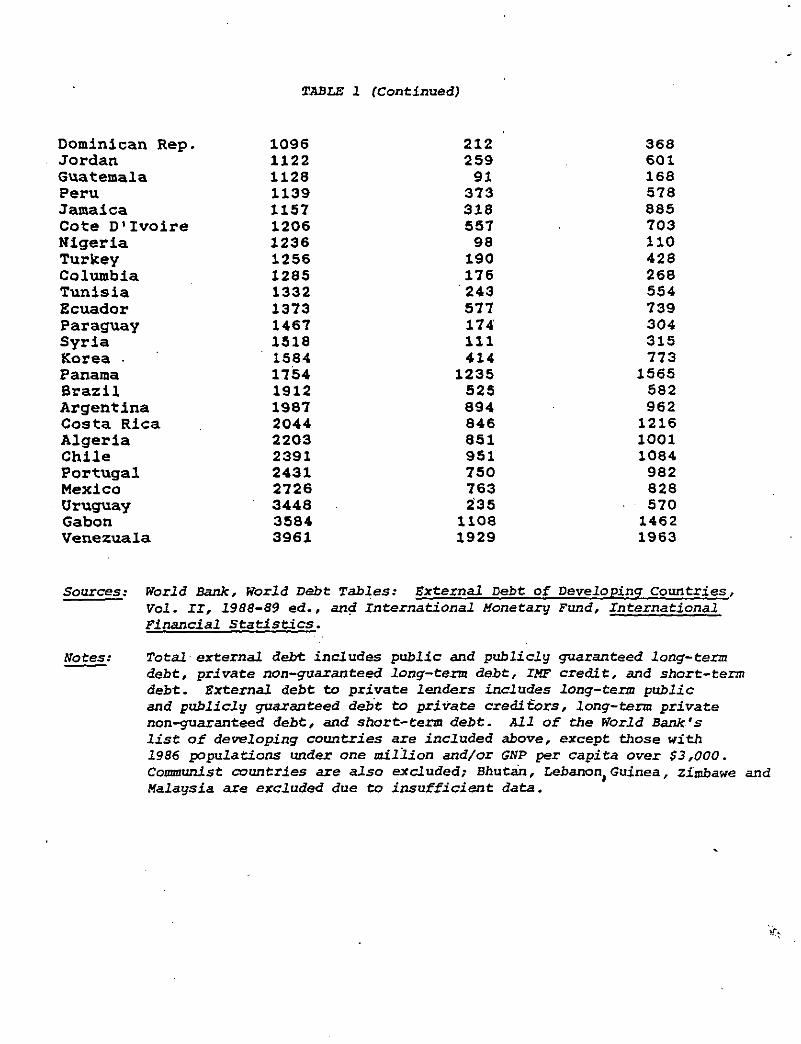
TABLE 1 (continued)

Dominican Rep. 1096 212 368Jordan 1122 259 601Guatemala 1128 91 168Peru 1139 373 578Jamaica 1157 318 885Cote D’Ivoire 1206 557 703Nigeria 1236 98 110Turkey U56 190 428Columbia 1285 176 268Tunisia 1.332 243 554Ecuador 1373 577 739Paraguay 1467 174 304Syria 1518 111 315Korea - 1584 414 773Panama 1754 1235 1565Brazil 1912 525 582Argentina 1987 894 962Costa Rica 2044 846 1216Algeria 2203 851 lOOiChile 2391 951 1084Portugal 2431 750 982Mexico 2726 763 828Uruguay 3448 235 570Gabon 3584 1108 1462Venezuala 3961 1929 1963

Sources: World Bank, World Debt Tables: External Debt of DesrelopLngCountries,Vol. II, 1988—89ed., and International Monetary Fund, InternationalFinancial Statistics.

Notes: Total external debt includes public and publicly guaranteed long-termdebt, private non-guaranteed long—ten debt, IMF credit, and short-termdebt. External debt to private lenders includes long-term publicand publicly guaranteed debt to private crediffors, long-term privatenon-guaranteed debt, and short-term debt. All of the World Bank’slist of developing countries are included above, except those with1986 ppulations under one million and/or GNP per capita over $3,000.Communistcountries are also excluded; Bhutan, Lebanon, Guinea, Zirnbawe andMalaysia are excluded due to insufficient data.

evidence that capital markets are less efficient in poorer countries (see, for

example, Goldsmith (1969) and McKlnnon (1973)).

In Table 1, we present 1980 data on income and external borrowing for

seventy developing countries, listed in order of GNP per capita. The second

column lists external debts owed to private lenders; the third column also

includes debts owed to other governmentsand to multilateral credit agencies

(e.g., the International Monetary Fund and the World Bank). A casual

comparison of column one with either column two or three indicates a strong

correlation between GUI’ and external borrowing. It is Important to note that

most of the external borrowing for countries in Table 1 took place over a

relatively short period (during the seventies). This rules one explanation of

the correlation, which is that the poorer countries are simply at an earlier

phase of their borrowing and development cycle. Another possibility is that

the countries that borrowed the most were the ones with the most favorable

productivity shocks. No doubt this is part of the explanation; we will make a

crude effort to control for productivity differentials. (Note though that a

pure productivity story is not capable of explaining differences in capital

market efficiency across countries.

Table 2 contains two sets of regressions, both using the log of GN? per

capita as the explanatory variable. In the first, the dependent variable is

the log of total external debt per capita. Over the entire sample,28 the

coefficient on GNP was 1.05, with a standard error of .08. Separate

regressions for Asia, Africa, and Latin America yield similar results. The

regional regressions can be Interpreted as one crude attempt to control for

28Nepal, which had zero private debt per capita, had to be excluded when theregressions were run in logs. Because it is poor, Nepal’s exclusion biasesthe estimated coefficients downwards.

22

TABLE 2

OLS Re&essionsof Debt/Capita on GNP/Capita tot Developing Countries:1980

log Total Fsernal Constant log GNP It Obse,vationsDebtperCapita per Capita

Allcountries 4.29 1.05 68 .73(.08)

Sub-Saharan -1.40 1.08 30 .60Africa (.16)

Latin America ~78 .97 - 19 .56and Caribbean (21)

Asia -2.36 1.20 10 .23(.19)

log .EuemalDebt Constant log GNP # Obseivadozu B2

to Ethate Lenders per Capitaper Capita

AflCountdes -524 1.60 68 .73(.12)

Sub-Saharan -5.20 1.51 30 .55Africa (.25)

Latin America -5.16 1.51 19 £2and Caribbean (.29)

AsIa -9.77 2.22. 10 .87(.30)

Africa: Bent,Botswana,Burldna Faso,Burundi, Canieroon,Central African Republi; Chad, Congo,Cote D’Ivoire, Ethiopia, Ghana, Kenya, Lesotho, Liberia, Madagascar, Malawi, Mali, Mauritania,Niger, Nigeria, Rwanda, Senegal, Sierra Leone,Somalia, Tanrinin, Toga, Uganda, Zaire,ZambIa.

Latin Americaand the Caribbean: Argentina,Bolivia, Brazil, Chile, Columbia, CostaRica, DominicanRepublic. Ecuador,El Salvador,Guatemala.Haiti, Honduras,Jamaica,Modco, Panama,Paraguay,Peru,Uruguay,VenezueLa.

Asia: Bangladesh, Burma, India, Indonesia,Korea, Pakistan,PapuaNew Guinea, Philippines,Sri Lanka, Thailand.

Other. Algeria. Egypt, Jordan, Morocco, Portugal, Syria, Tunisia, Turkey, Yemen Arab Republic.

differences in expected productivity across countries. The idea is that

whereas technology shocks may differ across Brazil and Nigeria, they are less

likely to differ betweenBrazil and Argentina.

One problem with using total external debt to measure country borrowing

is that the component consisting of official (public) debt Is probably best

viewed as foreign aid. Whereas most official debt is senior in principle, it

is junior to private debt in practice. Though technically, developing—country

debtors have promptly repaid official debt, in most cases official creditors

have made new loans in excess of any principal and interest repayments due.

[See Ruby and Rogoff (1988)].

In the second set of regressions reported In Table 2, the dependent

variable Includes only external debt owed to private creditors. Note that the

coefficients are always larger than one and the difference is significant over

the full sample.29 Again, this simple relation explains a very large share of

the variation in external borrowing across countries, and the coefficients are

relatively stable across regimes. We also ran a regression that included the

1980—1986 growth rate of per capita GNP as a proxy for expected productivity

change. This variable, however, was unimportant.30

We chose the year 1980 because after the debt crisis begart in 1982, the

correspondence between book value and the market value of loans becomes much

weaker.3’ There did not exist a secondarymarket for bank loans as of 1980,

29The results are quite robust to excluding trade credits and/or short termdebt from the regressions. However, when “Micronesian” countries withpopulations under one million are included, the coefficients become smallerand the standard errors larger.30 Obviously, it would be desirable to explore the dynamics of the external

debt—GNP relation more fully, but unfortunately short—term debt data for yearsprior to 1980 is suspect.311-iowever, the appendix presents similar regressions for the 1986 data, withsimilar results.

23

but most of the private loans were indexed to short—term interest rates. Thus

any capital gains or losses would mainly have to involve sovereign risk. The

fact that most debtor nations were still receiving new funds in 1980 suggests

that expectations of default were still quite low. Almost all sovereign debt

to private creditors is of equal priority (for a rationale see Bulow and

Ragoff (1988)), so countries can generally only get new loans only if their

old loans are valued near par.32

Vt. Conclusions

Across developing countries, capital market Inefficiencies tend to

decrease and external borrowing tends to sharply increase as wealth rises. We

have shown that a simple model of intertemporal trade under asymmetric

information can provide a coherent explanation of both these phenomenon,

without appealing to imperfect capital mobility.

Our empirical results that the elasticity of external borrowing [from

private creditors) with respect to income exceeds unity contradict the

conventional presumption that capital should flow from low marginal product of

capital rich countries to high marginal product of capital poor co~mtries.

To explain this result In isolation one can, of course, appeal to a

number of other theories. For example, the Marshall—Romermodel of growth

under increasing returns to scale is consistent with this phenomenon [see33

Romer (1989)1, and sovereign risk may also be part of the explanation.

320ur results do not include direct investment, since including this would notbe in the spirit of the asymmetric information model of section II. However,we note that within Africa and Asia, direct Investment was small relative todebt. For South America, it was somewhat larger, though still small relativeto debt.

Far recent bargaining—theoretic models of sovereign risk, see Eulow andRogoff (1989) or Fernandez and Rosenthal (1988). For a model combining

24

Cross—countrydifferences In productivity may also be relevant (although In

our empirical work we made a rough effort to control far this factor.) A

virtue of our explanation is that it is also consistent with evidence that

domestic capital markets operate less efficiently In developing countries.

Specifically, our model suggests that low—Income countries should have higher

spreads between loan and deposit rates.

Finally, we note that the present analysis suggests an alternative

explanation for the Feldstein—Horloka (1980) puzzle that savings and

investment tend to be highly correlated across countries. In a world of

perfect information, if a small country’s endowment Increases without any

corresponding increase in its productive opportunities, it will invest any

increased savings abroad. In a world where borrowing is subject to

Informational problems, however, a large part of the increase In savings may

be invested domestically.

sovereign risk and moral hazard, see Atkeson (1988).

25

APPENDIX

The formal problem which jointly determines how much the entrepreneur

invests and her contractual arrangement with lenders Is as follows: Choose k,

g bb, Z and 2 to solve

max — — [1 — z(kflt + rOt + b — k) (Al)

subject to

n(k)29+ [1 — = rb (AZ)

— (Z9— Zb)l = r (AS)

o~zb (A4)

W+b—k~O (AS)

Let p, ~‘, v, and i/i be the (non-negative) multipliers associated with (A2)

— (AS), respectively. Then the first-order necessary conditions with respect

g b

to k, b, Z and 2 are given by

—2

b) + ru”(k)/n’(k) —~‘ .O (AS)

= — 1) (A7)

— 1) — pr’(k) = 0 (AS)

[1 — — 1) + — ii = 0 tA9)

S

Recall that k is the first best level of capital investment, given by

‘C’

26

— r = 0 tAb)

(which corresponds to eq. (6) in the text). Then we have:

* * *

PRoposmoN 1: (1) If ‘vJ k , k = k ; (ii) If 14 < k , Ic < k

PROOF: Part (1) is obvious; since If ti � k the entrepreneur has sufficient

wealth to undertake the unconstrained optimal investment without borrowing;

she will lend any residual wealth. Part (11) can be proven by contradiction.

* *

Suppose S4 C Ic and k ~ Ic Then (AS) implies b >0. If b >0, then (AZ) and

(A4) imply2

g > ~ > then CA3) and (MO) imply Ic C k, which leads

to a contradiction. Q.E.D.

PROPOSITIoN 2: If W < k, k and2

g are given Jointly by

— = r (All)

= r(k — W)/ir(k) (A12)

where (All) and (A12) correspond to eqs. (9) and (10 ) in the text,

PROOF: If W < k then k < from Proposition 1. II k < then >

from (A3) and (MO). It follows from (A6) — (AS) that gi > 1. ThIs in turn

implies that ~-, t’, and ~ are positive. Thus (A4) and (As) hold with equality.

Using (A4) and (As) to eliminate and b front (A2) and (AS) yields (All) and

(A12). Q.E.D.

S *

COROLLARY: IIW<k, W<k<k.* *

PROOF: W C It implies k < k , from Proposition 1. Proposition 2 then

implies = 0. If k < and = 0, then2

g > o from (A)). It follows from

(A12) that Ic > W. Q.E.D.

27

CONPARATIVESTATICSOF THE TWO-COUNTRYCASE

From eqs. (22) and (23) In the text, and are determined Jointly by

the following two conditions:

p(kR,WR) = p(k~,W”) (81)

+ k”) = + W”) + (1-a)(W’~ + (82)

where

u’(k~)p(k3,W3) E p3

= J = P.R (83)

1 + u’(k3)[k3— W~1/u(k3)

so that C U and > 0.

Initially we assume that world wealth Is held constant at 14 (think of the

experiments as being wealth redistributiorts) so that CM) temporarily replaces

(82):

+ 1?) = CM)

where 14 is a fixed number. Then,

= — = — p/(pR + P > o (B5)

awB

~ +p”) <0 (B6)

Inspection of eq. (23) indicates that > 0 (since declines and V is

unchanged), and similarly > 0.ow

Next note that nattonal Income per capita for country J, is given by

= — r(k~ — wi)) +

28

= air(k)O + + — ak3] (B?)

Using the previous results In conjunction with CB7), one can readily determine

the impact of changes In and on the national Income of each country.

For example, it Is straightforward to show that a rise In may lower the

national income of the poor country, and definitely does so if the poor

country is a net debtor in the world capital market (i.e.. If +

(l_~))wJLl — < 0).

Now suppose the total stock of world endowment is permitted to change.

~B .RL .P .PLFor simplicity, let w = w and w = w , so that (82) becomes

~R+~PWR+4

ZP (88)

Then,

= + P)J~R + pP ) > ~ = + ~ ~ 4 ) ? (B9)

aw~ 2 1 1 1 ow 2 1

Under perfect informatIon, (88) together with eqs. (15) and (16) Imply that

akR ôk~— = — = 1/2a. Equation (B9) indicates that under asymmetric informationaw’~ awR

> 1/2a jf pP Is not too much smaller than pH or If pH Is sufficientlyown

large.34 The term in the numerator of (B9) reflects the influence of the

siphoning effect. If the siphoning effect is very strong is large),2 aw~

may be negative.

34Note that B = when = V.

29

T~tars Al

Measuresof External Borrowing Versus GNP: 1986

DOLLARS PER CAPITA

Grip External Debt Totalto Private Lenders External Debt

Ethiopia 116 9 49Bhutan . 132 0 16Bangladesh 152 3 78Chad 157 13 46Nepal 158 3 44Ma2apij 162 20 155Zaire 164 38 220Mall 183 16 206Tanzania 199 35 181ZambIa 204 232 815Burma 206 3 96Burlcina Paso 235 7 99Madagascar 236 46 285Burundi 257 10 114Uganda 275 9 •79GuInea 282 31 249Niger 285 87 230India 297 13 54Rwanda 304 6 70Sudan 308 142 431Toga 313 56 349Kenya 327 69 233Benin 332 122 226Pakistan 336 27 149Lesotho 343 8 119Cen. Afr. Rep. 344 19 166Sierra Leone 345 40 165Sri Lanka 389 61 252Somalia 395 54 485Ghana 398 32 189Mauritania 400 70 934Zimbabwe 415 190 669Haiti 415 21 130Indonesia 429 145 - 258Liberia 456 143 ~- 633Nigeria 468 179 248Senegal 531 88 456PhIlippines 543 344 515BolIvia 590 401 844Yemen A.R. 619 46 328Morocco 619 274 830Egypt 660 233 763Papua New Gui. 706 525 705Dominican Rep. 774 194 548El Salvador 779 58 349Thailand 786 200 356HondUras 792 223 662

TABLE Al (Continued)

cote D’tvoire 852 715 1097Guatemala 857 142 337Botswana 874 38 345Congo 907 1382 2079Jamaica 918 315 1709Paraguay 937 204 535Cameroon 989 168 351Ecuador 1050 641 956Turkey 1123 331 652Tunisia 1129 282 788ColumbIa 1155 293 526Chile 1211 1286 - 1641Jordan 1214 596 1179Peru 1314 480 790Mexico 1540 1072 1270Costa Rica 1540 958 1696Syria 1756 118 416Brazil 1940 634 814Uruguay 2000 986 1277Panama 2159 1462 2213Portugal 2248 1314 1604Korea 2288 822 1124Argentina 2397 1353 1602Gabon 2569 1009 1374Venezuala 2723 1903 1951klgeria 2752 723 857

Sources: world Bank, World Debt Tables: External Debt of Developingcountries, Vol. II, 1988—89 ed., and International Monetary

Fund, International Financial Statistics.

Notes: Total external debt includes public and publicly guaranteedlong—term debt, private nonguaranteedlong—terra debt, 11fFcredit, and short-term debt. External debt to private lendersincludes long-tent public and publicly-guaranteed debt to privatecreditors, private non—guaranteed long—term debt, and short—tenidebt. All of the World Bank’s list of developing countries areincluded above, except those with 1986 populations under onemillion and 1986 GYPs over $3,000. Cozwnunist countries areexcluded; Lebanon and Malaysia are excluded due to insufficientdata.

TABLE A2

OLS Regressionsof Debt/Capitaon CNJ’fCapifafor DeyelopintCountries: 1986

log Total Eternal Constant log (RIP # ObservationsDebtperCapita perCapita

All countries -.68 1.04 73 .67• (.09)

Sub-Saharan -.21 .99 33 .69Africa (.19)

Latin America -1.10 Lii 19 .58and Caribbean (.23)

Asia -3.09 1.38 12 .82(.20)

log ExternalDebt Constant log (RIP 9 Observationsto Private Lenders perCapitaper Capita

All Countries -6.35 L74 72 .72

(.13)

Sub-Saharan -5.05 1.54 33 .47Afzica (.29)

Latin America -tOS 2.00 19 .73and Caribbean (.29)

Asia -10.90 2.45 11 .83(.36)

Africa: Seniu, Botswaha, Burkina Paso, Burundi, Cameroon, Central African Republic Chad, Conga,

Cote D’Ivofre, Ethiopia, Ghana, Guinea, Kenya, Lesotho, Liberia, Madagascar, Malawi, Mali,Mauritania, Niger, Nigeria, Rwanda, Senegal, Sierra Leone, Somalia, Tanzania, Toga, Uganda,Zaire, Zambia, Zimbabwe.

Latin America and the Caribbean: Aigentina, Bolivia, Brazil, Chile, Columbia, Costa Rica,Dominican Republic, Ecuador, El Salvador, Guatemala, Haiti, Honduras, Jamaica, Mexico,

Panama, Paraguay, Peru, Uruguay, Venezuela.Asia: Bangladesh, Burma, India, thdonesia, Korea, Nepal, Pakistan, Papua New Guinea, Philippines.

Sri Lanka, Thailand.Other Algeria, Egypt, Jordan, Morocco, Portugal, Syria, Tunisia, Turkey, Yemen Arab Republic.

References

Atkeson, Andrew, ‘International Lending with Moral Hazard and Risk ofRepudiation, Stanford Graduate School of Business mlmeo, 1988.

Bernanke, Ben and Mark Gertler, “Agency Costs, Net Worth and BusinessFluctuations,” American Economic Review 79 (March 1989), 14—31.

Bulow, Jeremy and Kenneth Rogoff, “A Constant Recontracting Model of SovereignDebt,” Journal of Political Economy 97 (February 1989), 155—177.

_____________________________ “The Buyback Boondoggle,” BrookingsPaperson Economic Activity: no. 2 (1988), 675—698.

Dixit, Avinash, “Trade and Insurance with Moral Hazard,” Journal ofInternational Economics 23 (November 1987), 201-220.

Fazzari, Stephen, Glenn Hubbard and Bruce Petersen, “Financing Constraints andCorporate Investment,” Brookings Papers on Economic Activity: no. 1(1988), 141—195.

Felcisteth, Martin and Charles Horloka, “Domestic Saving and InternationalCapital Flows,” Economic Journal 90 (June 1980), 314—329.

Fernandez, Raquel and Robert Rosenthal, “Sovereign—Debt Renegotiations: AStrategic Analysis,’ NEER Working Paper No. 2597, (December 1988).

Frankel, Jeffrey and Alan MacArthur, “Political vs. Currency Premla inInternational Real Interest Rate Differentials,’ EuropeanEconomicReview 32 (1988), 1083-1121.

Gertler, Mark, ‘Financial Structure and Aggregate Economic Activity,” Journalof Money. Credit and Banking 20 (August 1988, Part 2), 559—588.

____________ “Financial Capacity, Reliquification and Production in anEconomy with Long—term Financial Arrangements,” NEER Working PaperNo. 2763 (November 1988).

Goldsmith, Raymond, Financial Structure and Development, (New Haven: YaleUniversity Press), 1969.

Greenwood, Jeremy and Stephen Williamson, “International FinancialIntermediation and Aggregate Fluctuations under Alternative ExchangeRate Regimes,” Journal of Monetary Economics 23 (Hay 1989), 401—431.

Hansen, James A.,” High Real Interest Rates and Spreads: An Introduction,” inHigh Interest Rates, Spreads,and the Costs of Intermediation, IndustryFinance Series Volume 18 (Washington: The World Bank), 1986.

Jensen, Michael and William Meckling, “Theory of the Firm: Managerial BehaviorAgency Costs and Ownership Structure,” Journal of Financial Economics 3(October 1976), 305—360.

30

Keynes, Joim Maynard, “The German Transfer Problem,’ Economic Journal 39(1929), 1—7.

K1etzer~ Kenneth and Bardhan, Pranhab, “Credit Markets and Patterns ofInternational Trade,” Journal of DevelopmentEconomics27 (October1987). 57—70.

McKlnnon, Ronald, Money and Capital In Economic Development, (Washington D.C.:The Brookings InstitutIon), 1973.

Obstfeld, Maurice, “Capital Mobility In the World Economy: Theory andMeasurement, in Karl Brunner and Allan H. Meltzer (eds. ), Carnegie—Rochester Conference Series on Public Policy 24 (Spring 1986), 55—103.

Ohlin, Bertel, “The GermanTransfer Problem: A Discussion,” Economic Journal39 (1929), 172—182.

Persson, Torsten and Lars Svenson, “Exchange Rate Variability and AssetTrade,” Journal of Monetary Economics 23 (May 1989) 485—509.

Rocha, Roberto de Rezende, “High Interest Rates, Spreads, and the Costs ofIntermediation,” In High Interest Rates. Spreads, and the Costs ofIntermediation. Industry and Finance Series Volume 18 (Washington: TheWorld Bank), 1986.

Romer, Paul, “Capital Accumulation in the Theory of Long Run Growth,”in Robert Barro (ed. ), Modern Business Cycle Theory (Cambridge: HarvardUniversity Press), 1989.

Samolyk, Katherine, “Spatially—Separated Banking Markets and Asset Swaps,” inEssays on Credit Flows and Macroeconomic Behavior, University ofWisconsin Ph.D. Dissertation (1988).

The World Bank, World Bank Development Report 1989: FInancial Systems andDevelopment (New York: Oxford University Press), 1989.

31