
MARINE ENVIRONMENT PROTECTION COMMITTEE … · MARINE ENVIRONMENT PROTECTION COMMITTEE 67th session...
40
I:\MEPC\67\6.doc E MARINE ENVIRONMENT PROTECTION COMMITTEE 67th session Agenda item 6 MEPC 67/6 1 July 2014 Original: ENGLISH REDUCTION OF GHG EMISSIONS FROM SHIPS Third IMO GHG Study 2014 – Executive Summary Note by the Secretariat SUMMARY Executive summary: This document contains in its annex the executive summary of the final report of the "Third IMO GHG Study 2014", which provides an update of the estimated GHG emissions for international shipping in the period 2007 to 2012. The complete final report can be found in document MEPC 67/INF.3. Strategic direction: 7.3 High-level action: 7.3.2 Planned output: 7.3.2.1 Action to be taken: Paragraph 11 Related documents: MEPC 67/INF.3; MEPC 66/21; MEPC 65/22, MEPC 65/22/Add.1; MEPC 64/23; MEPC 63/23; MEPC 59/4/7, MEPC 59/INF.10; MEPC 45/8; Circular Letter No.3381/Rev.1; resolution A.963(23) Background 1 The first IMO study on emission of greenhouse gases (GHG) from international shipping was commissioned following a request by the Diplomatic Conference on Air Pollution, held at IMO Headquarters in September 1997. The conference was convened by the Organization to consider air pollution issues related to international shipping and, more specifically, to adopt the 1997 Protocol to the MARPOL Convention (Annex VI: Regulations for the prevention of air pollution from ships). The first IMO study of greenhouse gas emissions from ships used figures for 1996 and was published in 2000 (MEPC 45/8). 2 Resolution A.963(23) on IMO policies and practices related to the reduction of greenhouse gas emissions from ships, adopted on 5 December 2003, urges the Committee to identify and develop the mechanism or mechanisms needed to achieve the limitation or reduction of GHG emissions from international shipping and, in doing so, to give priority, inter alia, to the establishment of a GHG emission baseline.
Transcript of MARINE ENVIRONMENT PROTECTION COMMITTEE … · MARINE ENVIRONMENT PROTECTION COMMITTEE 67th session...

I:\MEPC\67\6.doc
E
MARINE ENVIRONMENT PROTECTION COMMITTEE 67th session Agenda item 6
MEPC 67/6 1 July 2014
Original: ENGLISH
REDUCTION OF GHG EMISSIONS FROM SHIPS
Third IMO GHG Study 2014 – Executive Summary
Note by the Secretariat
SUMMARY
Executive summary: This document contains in its annex the executive summary of the final report of the "Third IMO GHG Study 2014", which provides an update of the estimated GHG emissions for international shipping in the period 2007 to 2012. The complete final report can be found in document MEPC 67/INF.3.
Strategic direction: 7.3
High-level action: 7.3.2
Planned output: 7.3.2.1
Action to be taken: Paragraph 11
Related documents: MEPC 67/INF.3; MEPC 66/21; MEPC 65/22, MEPC 65/22/Add.1; MEPC 64/23; MEPC 63/23; MEPC 59/4/7, MEPC 59/INF.10; MEPC 45/8; Circular Letter No.3381/Rev.1; resolution A.963(23)
Background 1 The first IMO study on emission of greenhouse gases (GHG) from international shipping was commissioned following a request by the Diplomatic Conference on Air Pollution, held at IMO Headquarters in September 1997. The conference was convened by the Organization to consider air pollution issues related to international shipping and, more specifically, to adopt the 1997 Protocol to the MARPOL Convention (Annex VI: Regulations for the prevention of air pollution from ships). The first IMO study of greenhouse gas emissions from ships used figures for 1996 and was published in 2000 (MEPC 45/8). 2 Resolution A.963(23) on IMO policies and practices related to the reduction of greenhouse gas emissions from ships, adopted on 5 December 2003, urges the Committee to identify and develop the mechanism or mechanisms needed to achieve the limitation or reduction of GHG emissions from international shipping and, in doing so, to give priority, inter alia, to the establishment of a GHG emission baseline.

MEPC 67/6 Page 2
I:\MEPC\67\6.doc
3 The "Second IMO GHG Study 2009" (MEPC 59/4/7 and MEPC 59/INF.10), commissioned as an update of the 2000 study, identified that international shipping was estimated to have emitted 870 million tonnes, or about 2.7% of the global emissions, of CO2 in 2007. Update of the Second IMO GHG Study 2009 4 MEPC 63 in March 2012 noted uncertainty in the estimates and projections of emissions from international shipping and agreed that further work should take place to provide the Committee with reliable and up-to-date information on which to base its decisions and requested the Secretariat to investigate possibilities and report to future sessions (MEPC 63/23, paragraph 5.58). 5 MEPC 64 in October 2012 endorsed, in principle, the outline for an update of the GHG emissions estimate, and, as agreed by the Committee (MEPC 64/23, paragraph 5.6), an Expert Workshop took place in February 2013 to further consider the methodology and assumptions to be used in the update. 6 MEPC 65 in May 2013, following consideration of the report of the Expert Workshop (MEPC 65/5/2), agreed to the terms of reference of the Update Study of the GHG emissions estimate from international shipping, including the establishment of a Steering Committee, as set out in the report of the Committee (MEPC 65/22, paragraph 5.7, and MEPC 65/22/Add.1, annex 19). 7 Financial contributions to enable the study to be undertaken were received from Australia, Denmark, Finland, Germany, Japan, the Netherlands, Norway, Sweden and the United Kingdom. The European Commission also contributed funds to support the work of IMO to address GHG emissions, including work in relation to the study. 8 Following MEPC 65, the Secretary-General established the Steering Committee, composed of the following Member States (Circular Letter No.3381/Rev.1): Belgium, Brazil, Canada, Chile, China, Finland, India, the Islamic Republic of Iran, Japan, Malaysia, the Marshall Islands, the Netherlands, Nigeria, Norway, the Republic of Korea, the Russian Federation, South Africa, Uganda, the United Kingdom and the United States. 9 The contract to undertake the study was awarded in October 2013 to an international consortium under the lead of UCL Consultants Ltd (UCLC). 10 MEPC 66, in noting the view of the Steering Committee members that the work was on track to meet the completion date and that the terms of reference of the study were being met, welcomed the progress made and also noted that the final report was expected to be considered at MEPC 67 (MEPC 66/21, paragraphs 5.3 and 5.6). Action requested of the Committee 11 The Committee is invited to approve the Third IMO GHG Study 2014 with a view to publication, recognizing that the responsibility for the scientific content of the study rests with the consortium, and to take action as appropriate.
***

MEPC 67/6 Annex, page 1
I:\MEPC\67\6.doc
ANNEX
Third IMO GHG Study 2014
Executive Summary Final Report, June 2014
Consortium members:
Data partners:

MEPC 67/6 Annex, page 2
I:\MEPC\67\6.doc
Executive Summary Contents Executive Summary Contents ................................................................................................ 2 Executive Summary Figures ................................................................................................... 3 Executive Summary Tables .................................................................................................... 4 Preface ................................................................................................................................... 5 List of abbreviations and acronyms ........................................................................................ 6 Key definitions ........................................................................................................................ 7 Executive Summary ............................................................................................................... 8 Key findings from the Third IMO GHG Study 2014 ............................................................. 8 Aim and objective of the study ......................................................................................... 13 Structure of the study and scope of work ......................................................................... 14 Summary of Section 1: Inventories of CO2 from international shipping ............................. 15 2012 fuel consumption and CO2 emissions by ship type ............................................. 15
2007–2012 fuel consumption by bottom-up and top-down methods: Third IMO GHG Study 2014 and Second IMO GHG Study 2009 ................................. 16
2007–2012 trends in CO2 emissions and drivers of emissions .................................... 20 Summary of Section 2: Inventories of GHGs and other relevant substances from international shipping ...................................................... 25 Summary of Section 3: Scenarios for shipping emissions ................................................ 28
Maritime transport demand projections ........................................................................ 28 Maritime emissions projections.................................................................................... 30
Summary of the data and methods used (Sections 1, 2 and 3) ........................................ 34 Key assumptions and method details .......................................................................... 34 Inventory estimation methods overview (Sections 1 and 2) ......................................... 34 Scenario estimation method overview (Section 3) ....................................................... 38

MEPC 67/6 Annex, page 3
I:\MEPC\67\6.doc
Executive Summary Figures Figure 1: Bottom-up CO2 emissions from international shipping by ship type 2012............... 15
Figure 2: Summary graph of annual fuel consumption broken down by ship type and machinery component (main, auxiliary and boiler) 2012. ...................................................... 16
Figure 3: CO2 emissions by ship type (international shipping only) calculated using the bottom-up method for all years (2007–2012). ....................................................................... 17
Figure 4: Summary graph of annual fuel use by all ships, estimated using the top-down and bottom-up methods, showing Second IMO GHG Study 2009 estimates and uncertainty ranges. ............................................................................................................... 18
Figure 5: Summary graph of annual fuel use by international shipping, estimated using the top-down and bottom-up methods, showing Second IMO GHG Study 2009 estimates and uncertainty ranges. ........................................................................................................ 18 Figure 6: Time series for trends in emissions and drivers of emissions in the oil tanker fleet 2007–2012. All trends are indexed to their values in 2007. ........................................... 20
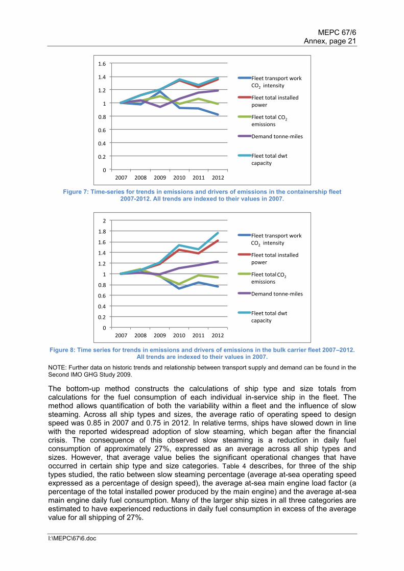
Figure 7: Time-series for trends in emissions and drivers of emissions in the containership fleet 2007–2012. All trends are indexed to their values in 2007. ........................................... 21
Figure 8: Time-series for trends in emissions and drivers of emissions in the bulk carrier fleet 2007–2012. All trends are indexed to their values in 2007. ................................ 21
Figure 9: Time series of bottom-up results for GHGs and other substances (all shipping). The green bar represents the Second IMO GHG Study 2009 estimate. ............................... 26
Figure 10: Time series of bottom-up results for GHGs and other substances (international shipping, domestic navigation and fishing). SOx values are preliminary and other adjustments may be made when fuel allocation results are finalized. ................................... 27
Figure 11: Historical data to 2012 on global transport work for non-coal combined bulk dry cargoes and other dry cargoes (billion tonne-miles) coupled to projections driven by GDPs from SSP1 through to SSP5 by 2050. .................................................................................. 29
Figure 12: Historical data to 2012 on global transport work for ship-transported coal and liquid fossil fuels (billion tonne-miles) coupled to projections of coal and energy demand driven by RCPs 2.6, 4.5, 6.0 and 8.5 by 2050. ..................................................................... 30
Figure 13: BAU projections of CO2 emissions from international maritime transport 2012-2050. ........................................................................................................................... 31
Figure 14: Projections of CO2 emissions from international maritime transport. Bold lines are BAU scenarios. Thin lines represent either greater efficiency improvement than BAU or additional emissions controls or both. ...................................................................... 31
Figure 15: Projections of CO2 emissions from international maritime transport under the same demand projections. Larger improvements in efficiency have a higher impact on CO2 emissions than a larger share of LNG in the fuel mix. ........................................................... 32
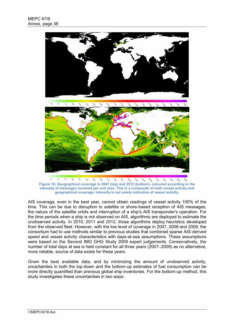
Figure 16: Geographical coverage in 2007 (top) and 2012 (bottom), coloured according to the intensity of messages received per unit area. This is a composite of both vessel activity and geographical coverage; intensity is not solely indicative of vessel activity. ......... 36
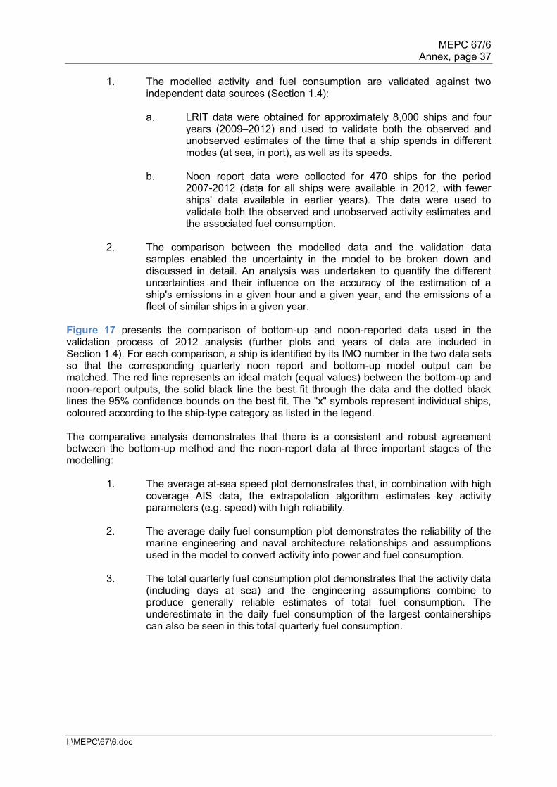
Figure 17: Total noon-reported quarterly fuel consumption of the main engine, compared with the bottom-up estimate over each quarter of 2012, with a filter to select only days with high reliability observations of the ship for 75% of the time or more...................................... 38

MEPC 67/6 Annex, page 4
I:\MEPC\67\6.doc
Executive Summary Tables Table 1: a) Shipping CO2 emissions compared with global CO2 (values in million tonnes CO2); and b) Shipping GHGs (in CO2e) compared with global GHGs (values in million tonnes CO2e). ........... 9
Table 2: International, domestic and fishing CO2 emissions 2007–2011, using top-down method. ................................................................................................................................ 19
Table 3: International, domestic and fishing CO2 emissions 2007–2012, using bottom-up method. ................................................................................................................................ 19
Table 4: Relationship between slow steaming, engine load factor (power output) and fuel consumption for 2007 and 2012. .......................................................................................... 23
Table 5: Summary of the scenarios for future emissions from international shipping, GHGs and other relevant substances. ............................................................................................. 33
Table 6: AIS observation statistics of the fleet identified in the IHSF database as in service in 2007 and 2012. ................................................................................................................. 35

MEPC 67/6 Annex, page 5
I:\MEPC\67\6.doc
Preface This study of greenhouse gas emissions from ships (hereafter the Third IMO GHG Study 2014) was commissioned as an update of the International Maritime Organization's (IMO) Second IMO GHG Study 2009. The updated study has been prepared on behalf of IMO by an international consortium led by the University College London (UCL) Energy Institute. The Third IMO GHG Study 2014 was carried out in partnership with the organizations and individuals listed below.
Consortium members, organizations and key individuals.
Organization Location Key individual(s)
UCL Energy Institute UK
Dr. Tristan Smith Eoin O'Keeffe Lucy Aldous Sophie Parker Carlo Raucci Michael Traut (visiting researcher)
Energy & Environmental Research Associates (EERA) USA Dr. James J. Corbett
Dr. James J. Winebrake Finnish Meteorological Institute (FMI) Finland Dr. Jukka-Pekka Jalkanen
Lasse Johansson
Starcrest USA Bruce Anderson Archana Agrawal Steve Ettinger
Civic Exchange Hong Kong, China Simon Ng Ocean Policy Research Foundation (OPRF) Japan Shinichi Hanayama
CE Delft The Netherlands Dr. Jasper Faber Dagmar Nelissen Maarten 't Hoen
Tau Scientific UK Professor David Lee exactEarth Canada Simon Chesworth Emergent Ventures India Ahutosh Pandey
The consortium thanks the Steering Committee of the Third IMO GHG Study 2014 for their helpful review and comments. The consortium acknowledges and thanks the following organizations for their invaluable data contributions to this study: exactEarth, IHS Maritime, Marine Traffic, Carbon Positive, Kystverket, Gerabulk, V.Ships and Shell. In the course of its efforts, the consortium gratefully received input and comments from the International Energy Agency (IEA), the International Association of Independent Tanker Owners (INTERTANKO), the International Chamber of Shipping (ICS), the World Shipping Council (WSC), the Port of Los Angeles, the Port of Long Beach, the Port Authority of New York & New Jersey, the Environmental Protection Department of the HKSAR Government and the Marine Department of the HKSAR Government. The views and conclusions expressed in this report are those of the authors. The recommended citation for this work is: Third IMO GHG Study 2014; International Maritime Organization (IMO) London, UK, June 2014; Smith, T. W. P.; Jalkanen, J. P.; Anderson, B. A.; Corbett, J. J.; Faber, J.; Hanayama, S.; O'Keeffe, E.; Parker, S.; Johansson, L.; Aldous, L.; Raucci, C.; Traut, M.; Ettinger, S.; Nelissen, D.; Lee, D. S.; Ng, S.; Agrawal, A.; Winebrake, J. J.; Hoen, M.; Chesworth, S.; Pandey, A.

MEPC 67/6 Annex, page 6
I:\MEPC\67\6.doc
List of abbreviations and acronyms AIS Automatic Identification System AR5 Fifth Assessment Report of the IPCC BAU business as usual BSFC brake-specific fuel consumption DG ENV Directorate-General for the Environment (European Commission) DOE Department of Energy (US) dwt deadweight tonnage ECA emission control area EEDI Energy Efficiency Design Index EEZ Exclusive Economic Zone EF emission factor EIA Environmental Investigation Agency EPA (US) Environmental Protection Agency FCF fuel correction factors FPSO floating production storage and offloading GDP gross domestic product GHG greenhouse gas gt gross tonnage GWP global warming potential (GWP100 represents the 100-year GWP) HCFC hydrochlorofluorocarbon HFC hydrofluorocarbon HFO heavy fuel oil HSD high speed diesel (engine) IAM integrated assessment models IEA International Energy Agency IFO intermediate fuel oil IHSF IHS Fairplay IMarEST Institute of Marine Engineering, Science and Technology IMO International Maritime Organization IPCC Intergovernmental Panel on Climate Change LNG liquid natural gas LRIT long-range identification and tracking (of ships) MACCs marginal abatement cost curves MCR maximum continuous revolution MDO marine diesel oil MEPC Marine Environment Protection Committee (IMO) MGO marine gas oil MMSI Maritime Mobile Service Identity MSD medium speed diesel (engine) nmi nautical mile NMVOC non-methane volatile organic compounds PCF perfluorocarbon PM particulate matter QA quality assurance QC quality control RCP representative concentration pathways S-AIS Satellite-based Automatic Identification System SEEMP Ship Energy Efficiency Management Plan SFOC specific fuel oil consumption SSD slow speed diesel (engine) SSP shared socioeconomic pathway UNEP United Nations Environment Programme UNFCCC United Nations Framework Convention on Climate Change VOC volatile organic compounds

MEPC 67/6 Annex, page 7
I:\MEPC\67\6.doc
Key definitions International shipping: shipping between ports of different countries, as opposed to domestic shipping. International shipping excludes military and fishing vessels. By this definition, the same ship may frequently be engaged in both international and domestic shipping operations. This is consistent with IPCC 2006 Guidelines (Second IMO GHG Study 2009). International marine bunker fuel: "[…] fuel quantities delivered to ships of all flags that are engaged in international navigation. The international navigation may take place at sea, on inland lakes and waterways, and in coastal waters. Consumption by ships engaged in domestic navigation is excluded. The domestic/international split is determined on the basis of port of departure and port of arrival, and not by the flag or nationality of the ship. Consumption by fishing vessels and by military forces is also excluded and included in residential, services and agriculture" (IEA website: http://www.iea.org/aboutus/glossary/i/). Domestic shipping: shipping between ports of the same country, as opposed to international shipping. Domestic shipping excludes military and fishing vessels. By this definition, the same ship may frequently be engaged in both international and domestic shipping operations. This definition is consistent with the IPCC 2006 Guidelines (Second IMO GHG Study 2009). Domestic navigation fuel: fuel delivered to vessels of all flags not engaged in international navigation (see the definition for international marine bunker fuel above). The domestic/international split should be determined on the basis of port of departure and port of arrival and not by the flag or nationality of the ship. Note that this may include journeys of considerable length between two ports in the same country (e.g. San Francisco to Honolulu). Fuel used for ocean, coastal and inland fishing and military consumption is excluded (http://www.iea.org/media/training/presentations/statisticsmarch/StatisticsofNonOECDCountries.pdf). Fishing fuel: fuel used for inland, coastal and deep-sea fishing. It covers fuel delivered to ships of all flags that have refuelled in the country (including international fishing) as well as energy used in the fishing industry (ISIC Division 03). Before 2007, fishing was included with agriculture/forestry and this may continue to be the case for some countries (http://www.iea.org/media/training/presentations/statisticsmarch/StatisticsofNonOECDCountries.pdf). Tonne: a metric system unit of mass equal to 1,000 kilograms (2,204.6 pounds) or 1 megagram (1 Mg). To avoid confusion with the smaller short ton and the slightly larger long ton, the tonne is also known as a metric ton; in this report, the tonne is distinguished by its spelling. Ton: a non-metric unit of mass considered to represent 907 kilograms (2,000 pounds), also sometimes called "short ton". In the United Kingdom the ton is defined as 1016 kilograms (2,240 pounds), also called "long ton". In this report, ton is used to imply "short ton" (907 kg) where the source cited used this term, and in calculations based on these sources (e.g. Section 2.1.3: Refrigerants, halogenated hydrocarbons and other non-combustion emissions).

MEPC 67/6 Annex, page 8
I:\MEPC\67\6.doc
Executive Summary
Key findings from the Third IMO GHG Study 2014
1. Shipping emissions during the period 2007–2012 and their significance relative to
other anthropogenic emissions.
1.1. For the year 2012, total shipping emissions were approximately 949 million tonnes CO2 and 972 million tonnes CO2e for GHGs combining CO2, CH4 and N2O. International shipping emissions for 2012 are estimated to be 796 million tonnes CO2 and 816 million tonnes CO2e for GHGs combining CO2, CH4 and N2O. International shipping accounts for approximately 2.2% and 2.1% of global CO2 and GHG emissions on a CO2 equivalent (CO2e) basis, respectively. Table 1 presents the full time series of shipping CO2 and CO2e emissions compared with global total CO2 and CO2e emissions.
For the period 2007–2012, on average, shipping accounted for
approximately 3.1% of annual global CO2 and approximately 2.8% of annual GHGs on a CO2e basis using 100-year global warming potential conversions from the AR5. A multi-year average estimate for all shipping using bottom-up totals for 2007–2012 is 1,016 million tonnes CO2 and 1,038 million tonnes CO2e for GHGs combining CO2, CH4 and N2O. International shipping accounts for approximately 2.6% and 2.4% of CO2 and GHGs on a CO2e basis, respectively. A multi-year average estimate for international shipping using bottom-up totals for 2007–2012 is 846 million tonnes CO2 and 866 million tonnes CO2e for GHGs combining CO2, CH4 and N2O. These multi-year CO2 and CO2e comparisons are similar to, but slightly smaller than, the 3.3% and 2.7% of global CO2 emissions reported by the Second IMO GHG Study 2009 for total shipping and international shipping in the year 2007, respectively.

MEPC 67/6 Annex, page 9
I:\MEPC\67\6.doc
Table 1 a) Shipping CO2 emissions compared with global CO2 (values in million tonnes CO2); and b) Shipping GHGs (in CO2e) compared with global GHGs (values in million tonnes CO2e).
Third IMO GHG Study 2014 CO2
Year Global CO21 Total shipping
% of global
International shipping % of global
2007 31,409 1,100 3.5% 885 2.8% 2008 32,204 1,135 3.5% 921 2.9% 2009 32,047 978 3.1% 855 2.7% 2010 33,612 915 2.7% 771 2.3% 2011 34,723 1,022 2.9% 850 2.4% 2012 35,640 949 2.7% 796 2.2%
Average 33,273 1,016 3.1% 846 2.6%
Third IMO GHG Study 2014 CO2e
Year Global CO2e2 Total shipping %of
global International shipping
%of global
2007 34,881 1,121 3.2% 903 2.6% 2008 35,677 1,157 3.2% 940 2.6% 2009 35,519 998 2.8% 873 2.5% 2010 37,085 935 2.5% 790 2.1% 2011 38,196 1,045 2.7% 871 2.3% 2012 39,113 972 2.5% 816 2.1%
Average 36,745 1,038 2.8% 866 2.4%
1.2. This study estimates multi-year (2007–2012) average annual totals of 20.9 million and 11.3 million tonnes for NOx (as NO2) and SOx (as SO2) from all shipping, respectively (corresponding to 6.3 million and 5.6 million tonnes converted to elemental weights for nitrogen and sulphur, respectively). NOx and SOx play indirect roles in tropospheric ozone formation and indirect aerosol warming at regional scales. International shipping is estimated to produce approximately 18.6 million and 10.6 million tonnes of NOx (as NO2) and SOx (as SO2) annually; this converts to totals of 5.6 million and 5.3 million tonnes of NOx and SOx (as elemental nitrogen and sulphur, respectively). Global NOx and SOx emissions from all shipping represent about 15% and 13% of global NOx and SOx from anthropogenic sources reported in the latest IPCC Assessment Report (AR5), respectively; international shipping NOx and SOx represent approximately 13% and 12% of global NOx and SOx totals, respectively.
1.3. Over the period 2007–2012, average annual fuel consumption ranged
between approximately 250 million and 325 million tonnes of fuel consumed by all ships within this study, reflecting top-down and bottom-up methods, respectively. Of that total, international shipping fuel consumption ranged between approximately 200 million and 270 million tonnes per year, depending on whether consumption was defined as fuel allocated to international voyages (top-down) or fuel used by ships engaged in international shipping (bottom-up), respectively.
1 Global comparator represents CO2 from fossil fuel consumption and cement production, converted from
Tg C y-1 to million metric tonnes CO2. Sources: Boden et al. 2013 for years 2007–2010; Peters et al. 2013 for years 2011–2012, as referenced in IPCC (2013).
2 Global comparator represents N2O from fossil fuels consumption and cement production. Source: IPCC (2013, Table 6.9).

MEPC 67/6 Annex, page 10
I:\MEPC\67\6.doc
1.4. Correlated with fuel consumption, CO2 emissions from shipping are estimated to range between approximately 740 million and 795 million tonnes per year in top-down results, and to range between approximately 900 million and 1150 million tonnes per year in bottom-up results. Both the top-down and the bottom-up methods indicate limited growth in energy and CO2 emissions from ships during 2007–2012, as suggested both by the IEA data and the bottom-up model. Nitrous oxide (N2O) emission patterns over 2007–2012 are similar to the fuel consumption and CO2 patterns, while methane (CH4) emissions from ships increased due to increased activity associated with the transport of gaseous cargoes by liquefied gas tankers, particularly during 2009–2012.
1.5. International shipping CO2 estimates range between approximately 595
million and 650 million tonnes calculated from top-down fuel statistics, and between approximately 775 million and 950 million tonnes according to bottom-up results. International shipping is the dominant source of the total shipping emissions of other GHGs: nitrous oxide (N2O) emissions from international shipping account for the majority (approximately 85%) of total shipping N2O emissions, and methane (CH4) emissions from international ships account for nearly all (approximately 99%) of total shipping emissions of CH4.
1.6. Refrigerant and air conditioning gas releases account for the majority of
HFC (and HCFC) emissions from ships. For older vessels, HCFCs (R-22) are still in service, whereas new vessels use HCFs (R134a/R404a). Use of SF6 and PCFs in ships is documented as rarely used in large enough quantities to be significant and is not estimated in this report.
1.7. Refrigerant and air conditioning gas releases from shipping contribute an
additional 15 million tons (range 10.8 million–19.1 million tons) in CO2 equivalent emissions. Inclusion of reefer container refrigerant emissions yields 13.5 million tons (low) and 21.8 million tons (high) of CO2 emissions.
1.8. Combustion emissions of SOx, NOx, PM, CO and NMVOCs are also
correlated with fuel consumption patterns, with some variability according to properties of combustion across engine types, fuel properties, etc., which affect emissions substances differently.
2. Resolution, quality and uncertainty of the emissions inventories.
2.1. The bottom-up method used in this study applies a similar approach to the
Second IMO GHG Study 2009 in order to estimate emissions from activity. However, instead of analysis carried out using ship type, size and annual average activity, calculations of activity, fuel consumption (per engine) and emissions (per GHG and pollutant substances) are performed for each in-service ship during each hour of each of the years 2007–2012, before aggregation to find the totals of each fleet and then of total shipping (international, domestic and fishing) and international shipping. This removes any uncertainty attributable to the use of average values and represents a substantial improvement in the resolution of shipping activity, energy demand and emissions data.
MEPC 67/6 Annex, page 11
I:\MEPC\67\6.doc
2.2. This study clearly demonstrates the confidence that can be placed in the detailed findings of the bottom-up method of analysis through both quality analysis and uncertainty analysis. Quality analysis includes rigorous testing of bottom-up results against noon reports and LRIT data. Uncertainty analysis quantifies, for the first time, the uncertainties in the top-down and the bottom-up estimates.
2.3. These analyses show that high-quality inventories of shipping emissions can be produced through the analysis of AIS data using models. Furthermore, the advancement in the state-of-the-art methods used in this study provides insight and produces new knowledge and understanding of the drivers of emissions within sub-sectors of shipping (ships of common type and size).
2.4. The quality analysis shows that the availability of improved data
(particularly AIS data) since 2010 has enabled the uncertainty of inventory estimates to be reduced (relative to previous years' estimates). However, uncertainties remain, particularly in the estimation of the total number of active ships and the allocation of ships or ship voyages between domestic and international shipping.
2.5. For both the top-down and the bottom-up inventory estimates in this study,
the uncertainties relative to the best estimate are not symmetrical (the likelihood of an overestimate is not the same as that of an underestimate). The top-down estimate is most likely to be an underestimate (for both total shipping and international shipping), for reasons discussed in the main report. The bottom-up uncertainty analysis shows that while the best estimate is higher than top-down totals, uncertainty is more likely to lower estimated values from the best estimate (again, for both total shipping and international shipping).
2.6. There is an overlap between the estimated uncertainty ranges of the
bottom-up and the top-down estimates of fuel consumption in each year and for both total shipping and international shipping. This provides evidence that the discrepancy between the top-down and the bottom-up best estimate value is resolvable through the respective methods' uncertainties.
2.7. Estimates of CO2 emissions from the top-down and bottom-up methods
converge over the period of the study as the source data of both methods improve in quality. This provides increased confidence in the quality of the methodologies and indicates the importance of improved AIS coverage from the increased use of satellite and shore-based receivers to the accuracy of the bottom-up method.
2.8. All previous IMO GHG studies have preferred activity-based (bottom-up)
inventories. In accordance with IPCC guidance, the statements from the MEPC Expert Workshop and the Second IMO GHG Study 2009, the Third IMO GHG Study 2014 consortium specifies the bottom-up best estimate as the consensus estimate for all years' emissions for GHGs and all pollutants.

MEPC 67/6 Annex, page 12
I:\MEPC\67\6.doc
3. Comparison of the inventories calculated in this study with the inventories of the Second 2009 IMO GHG study.
3.1. Best estimates for 2007 fuel use and CO2 emissions in this study agree
with the "consensus estimates" of the Second IMO GHG Study 2009 as they are within approximately 5% and approximately 4%, respectively.
3.2. Differences with the Second IMO GHG Study 2009 can be attributed to
improved activity data, better precision of individual vessel estimation and aggregation and updated knowledge of technology, emissions rates and vessel conditions. Quantification of uncertainties enables a fuller comparison of this study with previous work and future studies.
3.3. The estimates in this study of non-CO2 GHGs and some air pollutant
substances differ substantially from the 2009 results for the common year 2007. This study produces higher estimates of CH4 and N2O than the earlier study, higher by 43% and 40%, respectively (approximate values). The new study estimates lower emissions of SOx (approximately 30% lower) and approximately 40% of the CO emissions estimated in the 2009 study.
3.4. Estimates for NOx, PM and NMVOC in both studies are similar for 2007,
within 10%, 11% and 3%, respectively (approximate values).
4. Fuel use trends and drivers in fuel use (2007–2012), in specific ship types. 4.1. The total fuel consumption of shipping is dominated by three ship types: oil
tankers, containerships and bulk carriers. Consistently for all ship types, the main engines (propulsion) are the dominant fuel consumers.
4.2. Allocating top-down fuel consumption to international shipping can be done
explicitly, according to definitions for international marine bunkers. Allocating bottom-up fuel consumption to international shipping required application of a heuristic approach. The Third IMO GHG Study 2014 used qualitative information from AIS to designate larger passenger ferries (both passenger-only Pax ferries and vehicle-and-passenger RoPax ferries) as international cargo transport vessels. Both methods are unable to fully evaluate global domestic fuel consumption.
4.3. The three most significant sectors of the shipping industry from a CO2
perspective (oil tankers, containerships and bulk carriers) have experienced different trends over the period of this study (2007–2012). All three contain latent emissions increases (suppressed by slow steaming and historically low activity and productivity) that could return to activity levels that create emissions increases if the market dynamics that informed those trends revert to their previous levels.
4.4. Fleet activity during the period 2007–2012 demonstrates widespread
adoption of slow steaming. The average reduction in at-sea speed relative to design speed was 12% and the average reduction in daily fuel consumption was 27%. Many ship type and size categories exceeded this average. Reductions in daily fuel consumption in some oil tanker size categories was approximately 50% and some container ship size categories reduced energy use by more than 70%. Generally, smaller ship size categories operated without significant change over the period, also evidenced by more consistent fuel consumption and voyage speeds.

MEPC 67/6 Annex, page 13
I:\MEPC\67\6.doc
4.5. A reduction in speed and the associated reduction in fuel consumption do not relate to an equivalent percentage increase in efficiency, because a greater number of ships (or more days at sea) are required to do the same amount of transport work.
5. Future scenarios (2012–2050).
5.1. Maritime CO2 emissions are projected to increase significantly in the
coming decades. Depending on future economic and energy developments, this study's BAU scenarios project an increase by 50% to 250% in the period to 2050. Further action on efficiency and emissions can mitigate the emissions growth, although all scenarios but one project emissions in 2050 to be higher than in 2012.
5.2. Among the different cargo categories, demand for transport of unitized
cargoes is projected to increase most rapidly in all scenarios. 5.3. Emissions projections demonstrate that improvements in efficiency are
important in mitigating emissions increase. However, even modelled improvements with the greatest energy savings could not yield a downward trend. Compared to regulatory or market-driven improvements in efficiency, changes in the fuel mix have a limited impact on GHG emissions, assuming that fossil fuels remain dominant.
5.4. Most other emissions increase in parallel with CO2 and fuel, with some
notable exceptions. Methane emissions are projected to increase rapidly (albeit from a low base) as the share of LNG in the fuel mix increases. Emissions of nitrogen oxides increase at a lower rate than CO2 emissions as a result of Tier II and Tier III engines entering the fleet. Emissions of particulate matter show an absolute decrease until 2020, and sulphurous oxides continue to decline through 2050, mainly because of MARPOL Annex VI requirements on the sulphur content of fuels.
Aim and objective of the study This study provides IMO with a multi-year inventory and future scenarios for GHG and non-GHG emissions from ships. The context for this work is:
The IMO committees and their members require access to up-to-date information to support working groups and policy decision-making. Five years have passed since the publication of the previous study (Second IMO GHG Study 2009), which estimated emissions for 2007 and provided scenarios from 2007 to 2050. Furthermore, the IPCC has updated its analysis of future scenarios for the global economy in its AR5 (2013), including mitigation scenarios. IMO policy developments, including MARPOL Annex VI amendments for EEDI and SEEMP, have also occurred since the 2009 study was undertaken. In this context, the Third IMO GHG Study 2014 updates the previous work by producing yearly inventories since 2007.
MEPC 67/6 Annex, page 14
I:\MEPC\67\6.doc
Other studies published since the Second IMO GHG Study 2009 have indicated that one impact of the global financial crisis may have been to modify previously reported trends, both in demand for shipping and in the intensity of shipping emissions. This could produce significantly different recent-year emissions than the previously forecasted scenarios, and may modify the long-run projections for 2050 ship emissions. In this context, the Third IMO GHG Study 2014 provides new projections informed by important economic and technological changes since 2007.
Since 2009, greater geographical coverage achieved via satellite
technology/AIS receivers has improved the quality of data available to characterize shipping activity beyond the state of practice used in the Second IMO GHG Study 2009. These new data make possible more detailed methods that can substantially improve the quality of bottom-up inventory estimates. Additionally, improved understanding of marine fuel (bunker) statistics reported by nations has identified, but not quantified, potential uncertainties in the accuracy of top-down inventory estimates from fuel sales to ships. Improved bottom-up estimates can reconcile better the discrepancies between top-down and bottom-up emissions observed in previous studies (including the Second IMO GHG Study 2009). In this context, the Third IMO GHG Study 2014 represents the most detailed and comprehensive global inventory of shipping emissions to date.
The scope and design of the Third IMO GHG Study 2014 responds directly to specific directives from the IMO Secretariat that derived from the IMO Expert Workshop (2013) recommendations with regard to activity-based (bottom-up) ship emissions estimation. These recommendations were:
to consider direct vessel observations to the greatest extent possible; to use vessel-specific activity and technical details in a bottom-up inventory
model; to use "to the best extent possible" actual vessel speed to obtain engine loads.
The IMO Expert Workshop recognised that "bottom-up estimates are far more detailed and are generally based on ship activity levels by calculating the fuel consumption and emissions from individual ship movements" and that "a more sophisticated bottom-up approach to develop emission estimates on a ship-by-ship basis" would "require significant data to be inputted and may require additional time […] to complete". Structure of the study and scope of work The Third IMO GHG Study 2014 report follows the structure of the terms of reference for the work, which comprise three main sections: Section 1: Inventories of CO2 emissions from international shipping 2007–2012 This section deploys both a top-down (2007–2011) and a bottom-up (2007–2012) analysis of CO2 emissions from international shipping. The inventories are analysed and discussed with respect to the quality of methods and data and to uncertainty of results. The discrepancies between the bottom-up and top-down inventories are discussed. The Third IMO GHG Study 2014 inventory for 2007 is compared to the Second IMO GHG Study 2009 inventory for the same year.
MEPC 67/6 Annex, page 15
I:\MEPC\67\6.doc
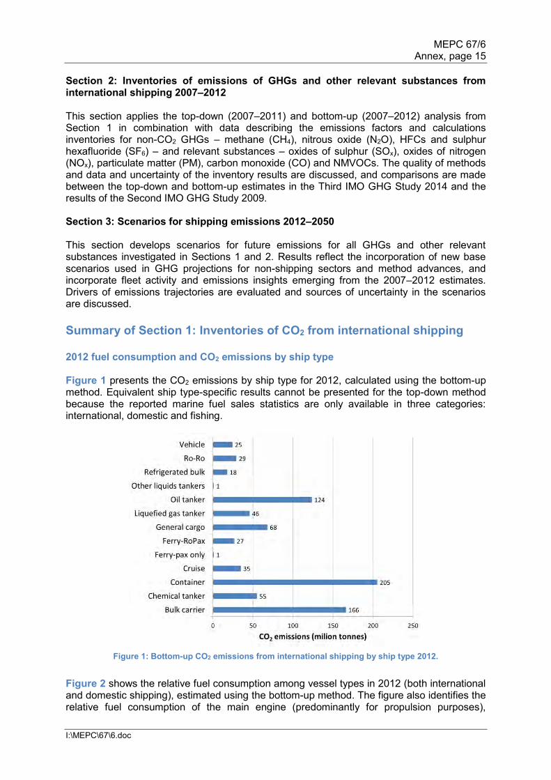
Section 2: Inventories of emissions of GHGs and other relevant substances from international shipping 2007–2012 This section applies the top-down (2007–2011) and bottom-up (2007–2012) analysis from Section 1 in combination with data describing the emissions factors and calculations inventories for non-CO2 GHGs – methane (CH4), nitrous oxide (N2O), HFCs and sulphur hexafluoride (SF6) – and relevant substances – oxides of sulphur (SOx), oxides of nitrogen (NOx), particulate matter (PM), carbon monoxide (CO) and NMVOCs. The quality of methods and data and uncertainty of the inventory results are discussed, and comparisons are made between the top-down and bottom-up estimates in the Third IMO GHG Study 2014 and the results of the Second IMO GHG Study 2009. Section 3: Scenarios for shipping emissions 2012–2050 This section develops scenarios for future emissions for all GHGs and other relevant substances investigated in Sections 1 and 2. Results reflect the incorporation of new base scenarios used in GHG projections for non-shipping sectors and method advances, and incorporate fleet activity and emissions insights emerging from the 2007–2012 estimates. Drivers of emissions trajectories are evaluated and sources of uncertainty in the scenarios are discussed. Summary of Section 1: Inventories of CO2 from international shipping 2012 fuel consumption and CO2 emissions by ship type Figure 1 presents the CO2 emissions by ship type for 2012, calculated using the bottom-up method. Equivalent ship type-specific results cannot be presented for the top-down method because the reported marine fuel sales statistics are only available in three categories: international, domestic and fishing.
Figure 1: Bottom-up CO2 emissions from international shipping by ship type 2012.
Figure 2 shows the relative fuel consumption among vessel types in 2012 (both international and domestic shipping), estimated using the bottom-up method. The figure also identifies the relative fuel consumption of the main engine (predominantly for propulsion purposes),

MEPC 67/6 Annex, page 16
I:\MEPC\67\6.doc
auxiliary engine (normally for electricity generation) and the boilers (for steam generation). The total shipping fuel consumption is shown in 2012 to be dominated by three ship types: oil tankers, bulk carriers and containerships. In each of those ship types, the main engine consumes the majority of the fuel.
Figure 2: Summary graph of annual fuel consumption broken down by ship type and machinery
component (main, auxiliary and boiler) 2012.
2007–2012 fuel consumption by bottom-up and top-down methods: Third IMO GHG Study 2014 and Second IMO GHG Study 2009 Figure 3 shows the year-on-year trends for the total CO2 emissions of each ship type, as estimated using the bottom-up method. Figure 4 and Figure 5 show the associated total fuel consumption estimates for all years of the study, from both the top-down and bottom-up methods. The total CO2 emissions aggregated to the lowest level of detail in the top-down analysis (international, domestic and fishing) are presented in Table 2 and Table 3. Figure 4 and Figure 3 present results from the 2014 study (all years) and from the Second IMO GHG Study 2009 (2007 only). The comparison of the estimates in 2007 shows that using both the top-down and the bottom-up analysis methods, the results of the Third IMO GHG Study 2014 for the total fuel inventory and the international shipping estimate are in close agreement with the findings from the Second IMO GHG Study 2009. Further analysis and discussion of the comparison between the two studies is undertaken in Section 1.6 of this report.

MEPC 67/6 Annex, page 17
I:\MEPC\67\6.doc
Figure 3: CO2 emissions by ship type (international shipping only) calculated using the bottom-up
method for all years (2007–2012).
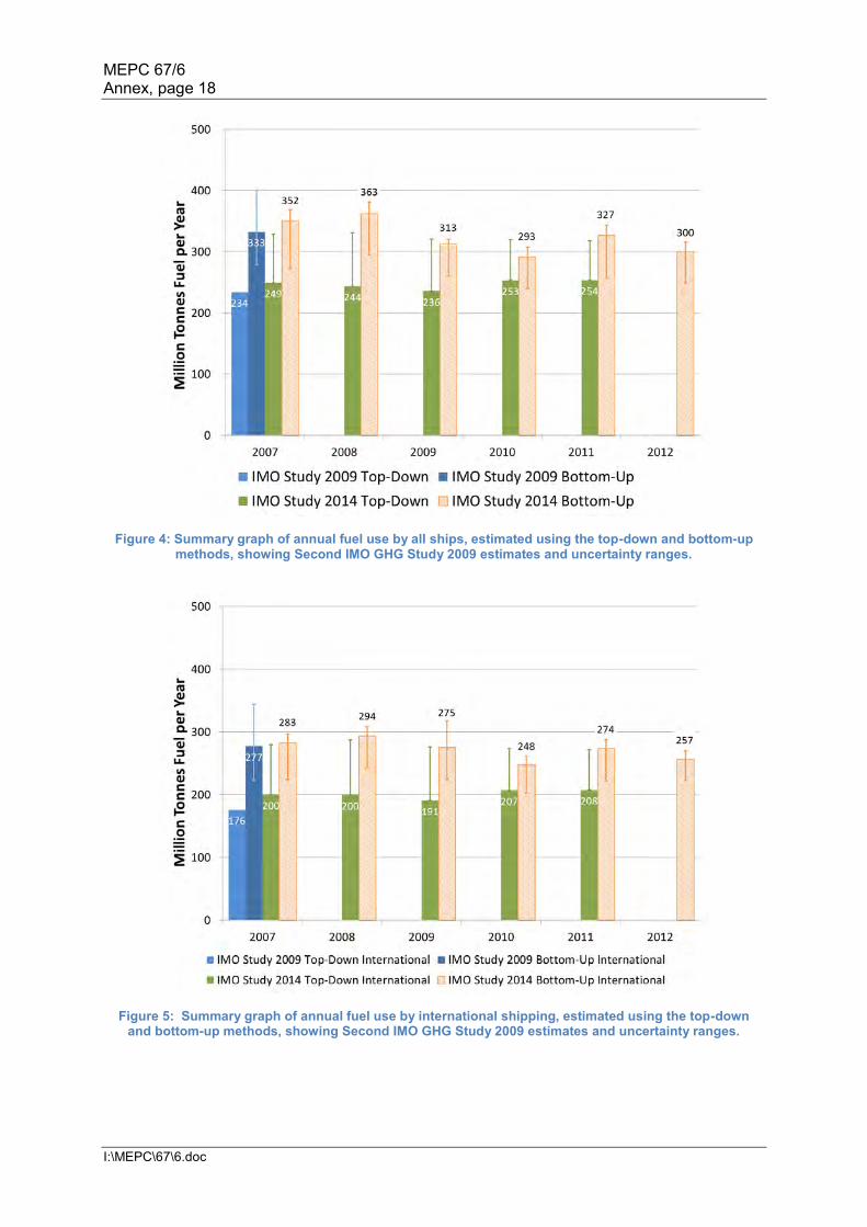
The vertical bar attached to the total fuel consumption estimate for each year and each method represents the uncertainty in the estimates. For the bottom-up method, this error bar is derived from a Monte Carlo simulation of the most important input parameters to the calculation. The most important sources of uncertainty in the bottom-up method results are the number of days a ship spends at sea per year (attributable to incomplete AIS coverage of a ship's activity) and the number of ships that are active (in-service) in a given year (attributable to the discrepancy between the difference between the number of ships observed in the AIS data and the number of ships described as in-service in the IHSF database). The top-down estimates are also uncertain, including observed discrepancies between global imports and exports of fuel oil and distillate oil, observed transfer discrepancies among fuel products that can be blended into marine fuels, and potential for misallocation of fuels between sectors of shipping (international, domestic and fishing). Neither the top-down nor the bottom-up uncertainties are symmetric, showing that uncertainty in the top-down best estimate is more likely to increase the estimate of fuel consumption from the best estimate, and that uncertainty in bottom-up best-estimate value is more likely to lower estimated values from the best estimate. Differences between the bottom-up and the top-down best-estimate values in this study are consistent with the differences observed in the Second IMO GHG Study 2009. This convergence of best estimates is important because, in conjunction with the quality (Section 1.4) and uncertainty (Section 1.5) analysis, it provides evidence that increasing confidence can be placed in both analytical approaches.
MEPC 67/6 Annex, page 18
I:\MEPC\67\6.doc
Figure 4: Summary graph of annual fuel use by all ships, estimated using the top-down and bottom-up methods, showing Second IMO GHG Study 2009 estimates and uncertainty ranges.
Figure 5: Summary graph of annual fuel use by international shipping, estimated using the top-down and bottom-up methods, showing Second IMO GHG Study 2009 estimates and uncertainty ranges.
MEPC 67/6 Annex, page 19
I:\MEPC\67\6.doc
Table 2: International, domestic and fishing CO2 emissions 2007–2011, using top-down method.
Marine sector Fuel type 2007 2008 2009 2010 2011
International shipping HFO 542.1 551.2 516.6 557.1 554.0 MDO 83.4 72.8 79.8 90.4 94.9 NG 0.0 0.0 0.0 0.0 0.0
Top-down international total All 625.5 624.0 596.4 647.5 648.9
Domestic navigation HFO 62.0 44.2 47.6 44.5 39.5 MDO 72.8 76.6 75.7 82.4 87.8 NG 0.1 0.1 0.1 0.1 0.2
Top-down domestic total All 134.9 121.0 123.4 127.1 127.6
Fishing HFO 3.4 3.4 3.1 2.5 2.5 MDO 17.3 15.7 16.0 16.7 16.4 NG 0.1 0.1 0.1 0.1 0.1
Top-down fishing total All 20.8 19.2 19.3 19.2 19.0 All fuels top-down 781.2 764.1 739.1 793.8 795.4
Table 3: International, domestic and fishing CO2 emissions 2007–2012, using bottom-up method.
Marine sector Fuel type 2007 2008 2009 2010 2011 2012
HFO 773.8 802.7 736.6 650.6 716.9 667.9 International shipping MDO 97.2 102.9 104.2 102.2 109.8 105.2 NG 13.9 15.4 14.2 18.6 22.8 22.6 Bottom-up international total All 884.9 920.9 855.1 771.4 849.5 795.7 HFO 53.8 57.4 32.5 45.1 61.7 39.9 Domestic navigation MDO 142.7 138.8 80.1 88.2 98.1 91.6 NG 0 0 0 0 0 0 Bottom-up domestic total All 196.5 196.2 112.6 133.3 159.7 131.4 HFO 1.6 1.5 0.9 0.8 1.4 1.1 Fishing MDO 17.0 16.4 9.3 9.2 10.9 9.9 NG 0 0 0 0 0 11 Bottom-up fishing total All 18.6 18.0 10.2 10.0 12.3 22.0
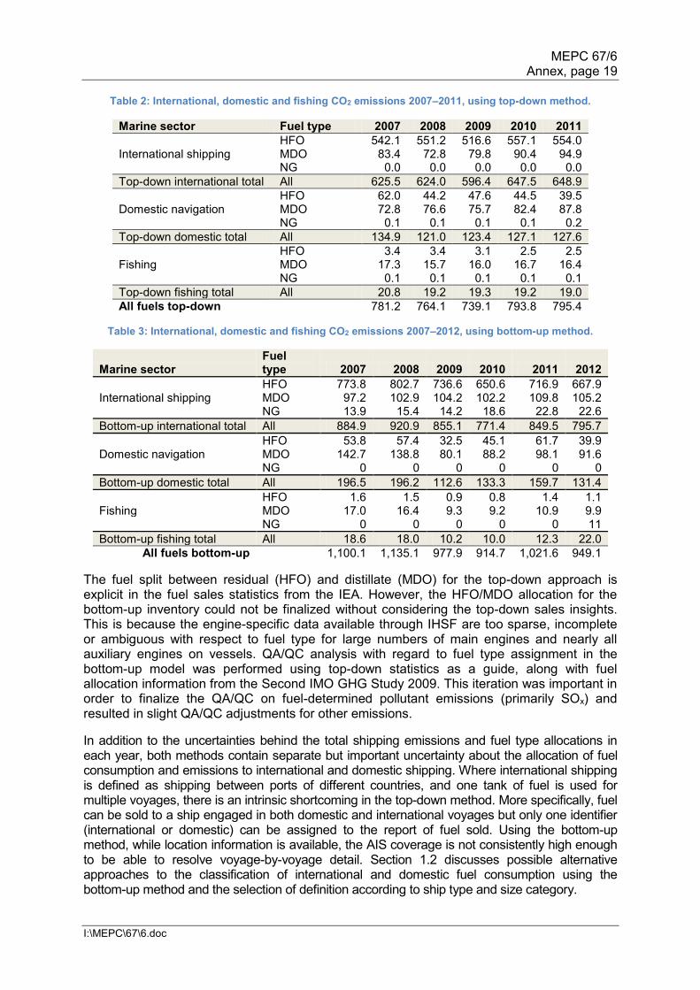
All fuels bottom-up 1,100.1 1,135.1 977.9 914.7 1,021.6 949.1 The fuel split between residual (HFO) and distillate (MDO) for the top-down approach is explicit in the fuel sales statistics from the IEA. However, the HFO/MDO allocation for the bottom-up inventory could not be finalized without considering the top-down sales insights. This is because the engine-specific data available through IHSF are too sparse, incomplete or ambiguous with respect to fuel type for large numbers of main engines and nearly all auxiliary engines on vessels. QA/QC analysis with regard to fuel type assignment in the bottom-up model was performed using top-down statistics as a guide, along with fuel allocation information from the Second IMO GHG Study 2009. This iteration was important in order to finalize the QA/QC on fuel-determined pollutant emissions (primarily SOx) and resulted in slight QA/QC adjustments for other emissions. In addition to the uncertainties behind the total shipping emissions and fuel type allocations in each year, both methods contain separate but important uncertainty about the allocation of fuel consumption and emissions to international and domestic shipping. Where international shipping is defined as shipping between ports of different countries, and one tank of fuel is used for multiple voyages, there is an intrinsic shortcoming in the top-down method. More specifically, fuel can be sold to a ship engaged in both domestic and international voyages but only one identifier (international or domestic) can be assigned to the report of fuel sold. Using the bottom-up method, while location information is available, the AIS coverage is not consistently high enough to be able to resolve voyage-by-voyage detail. Section 1.2 discusses possible alternative approaches to the classification of international and domestic fuel consumption using the bottom-up method and the selection of definition according to ship type and size category.

MEPC 67/6 Annex, page 20
I:\MEPC\67\6.doc
Particular care must be taken when interpreting the domestic fuel consumption and emissions estimates from both the top-down and the bottom-up methods. Depending on where the fuel for domestic shipping and fishing is bought, it may or may not be adequately captured in the IEA marine bunkers. For example, inland or leisure and fishing vessels may purchase fuel at locations where fuel is also sold to other sectors of the economy and therefore it may be misallocated. In the bottom-up method, fuel consumption is only included for ships that appear in the IHSF database (and have an IMO number). While this should cover all international shipping, many domestic vessels (inland, fishing or cabotage) may not be included in this database. An indication of the number of vessels excluded from the bottom-up method was obtained from the count of MMSI numbers observed on the AIS for which no match with the IHSF database was obtained. The implications of this count for both the bottom-up and top-down analyses are discussed in Section 1.4.
2007–2012 trends in CO2 emissions and drivers of emissions Figure 6, Figure 7 and Figure 8 present indexed time series of the total CO2 emissions during the period studied for three ship types: oil tankers, containerships and bulk carriers (all in-service ships). The figures also present several key drivers of CO2 emissions that can be used to decompose the fleet, activity and CO2 emission trends, estimated using the bottom-up method. All trends are indexed to their values in 2007. Despite rising transport demand in all three fleets, each fleet's total emissions are shown either to remain approximately constant or to decrease slightly. The contrast between the three plots in Figures 6–8 shows that these three sectors of the shipping industry have experienced different changes over the period 2007–2012. The oil tanker sector has reduced its emissions by a total of 20%. During the same period the dry bulk and container ship sectors also saw absolute emissions reductions but by smaller amounts. All ship types experienced similar reductions in average annual fuel consumption but differences in the number of ships in service, which explains the difference in fleet total CO2 emissions trends. The reduction in average days at sea during the period studied is greatest in the dry bulk fleet, while the container ship fleet has seen a slight increase. Consistent with the results presented in Table 4, containerships adopted slow steaming more than any other ship type. So, over the same period of time, similar reductions in average fuel consumption per ship have come about through different combinations of slow steaming and days at sea.
0
0.2
0.4
0.6
0.8
1
1.2
1.4
2007 2008 2009 2010 2011 2012
FleettransportworkCO2intensity
Fleettotalinstalledpower
FleettotalCO2emissions
Demandtonne-miles
Fleettotaldwtcapacity
CO2
CO2
Figure 6 Time-series for trends in emissions and drivers of emissions in the oil tanker fleet 2007–2012. All
trends are indexed to their values in 2007.
MEPC 67/6 Annex, page 21
I:\MEPC\67\6.doc
0
0.2
0.4
0.6
0.8
1
1.2
1.4
1.6
2007 2008 2009 2010 2011 2012
FleettransportworkCO2intensity
Fleettotalinstalledpower
FleettotalCO2emissions
Demandtonne-miles
Fleettotaldwtcapacity
CO2
CO2
Figure 7: Time-series for trends in emissions and drivers of emissions in the containership fleet
2007-2012. All trends are indexed to their values in 2007.
0
0.2
0.4
0.6
0.8
1
1.2
1.4
1.6
1.8
2
2007 2008 2009 2010 2011 2012
FleettransportworkCO2intensity
Fleettotalinstalledpower
FleettotalCO2emissions
Demandtonne-miles
Fleettotaldwtcapacity
CO2
CO2
Figure 8: Time series for trends in emissions and drivers of emissions in the bulk carrier fleet 2007–2012.
All trends are indexed to their values in 2007.
NOTE: Further data on historic trends and relationship between transport supply and demand can be found in the Second IMO GHG Study 2009. The bottom-up method constructs the calculations of ship type and size totals from calculations for the fuel consumption of each individual in-service ship in the fleet. The method allows quantification of both the variability within a fleet and the influence of slow steaming. Across all ship types and sizes, the average ratio of operating speed to design speed was 0.85 in 2007 and 0.75 in 2012. In relative terms, ships have slowed down in line with the reported widespread adoption of slow steaming, which began after the financial crisis. The consequence of this observed slow steaming is a reduction in daily fuel consumption of approximately 27%, expressed as an average across all ship types and sizes. However, that average value belies the significant operational changes that have occurred in certain ship type and size categories. Table 4 describes, for three of the ship types studied, the ratio between slow steaming percentage (average at-sea operating speed expressed as a percentage of design speed), the average at-sea main engine load factor (a percentage of the total installed power produced by the main engine) and the average at-sea main engine daily fuel consumption. Many of the larger ship sizes in all three categories are estimated to have experienced reductions in daily fuel consumption in excess of the average value for all shipping of 27%.
MEPC 67/6 Annex, page 22
I:\MEPC\67\6.doc
Table 4 also shows that the ships with the highest design speeds (containerships) have adopted the greatest levels of slow steaming (in many cases operating at average speeds that are 60–70% of their design speeds), relative to oil tankers and bulk carriers. Referring back to Figure 8, it can be seen that for bulk carriers, the observed trend in slow steaming is not concurrent with the technical specifications of the ships remaining constant. For example, the largest bulk carriers (200,000+ dwt capacity) saw increases in average size (dwt capacity) as well as increased installed power (from an average of 18.9 MW to 22.2 MW), as a result of a large number of new ships entering the fleet over the period studied. (The fleet grew from 102 ships in 2007 to 294 ships in 2012.) The analysis of trends in speed and days at sea is consistent with the findings in Section 3 that the global fleet is currently at or near the historic low in terms of productivity (transport work per unit of capacity). The consequence is that these (and many other) sectors of the shipping industry represent latent emissions increases, because the fundamentals (number of ships in service) have seen upward trends that have been offset as economic pressures act to reduce productivity (which in turn reduces emissions intensity). Whether and when the latent emissions may appear is uncertain, as it depends on the future market dynamics of the industry. However, the risk is high that the fleet could encounter conditions favouring the conversion of latent emissions to actual emissions; this could mean that shipping reverts to the trajectory estimated in the Second IMO GHG Study 2009. This upward potential is quantified as part of sensitivity analysis in Section 3. A reduction in speed and the associated reduction in fuel consumption do not relate to an equivalent percentage increase in efficiency, because a greater number of ships (or more days at sea) are required to do the same amount of transport work. This relationship is discussed in greater detail in Section 3.

MEPC 67/6 Annex, page 23
I:\MEPC\67\6.doc
Table 4: Relationship between slow steaming, engine load factor (power output) and fuel consumption for 2007 and 2012.
Ship type Size category Units
2007 2012
% change in average at-sea tonnes per day (tpd) 2007-2012
Ratio of average at-sea speed to design speed
Average at-sea main engine load factor (% MCR)
At-sea consumption in tonnes per day
Ratio of average at-sea speed to design speed
Average at-sea main engine load factor (% MCR)
At-sea consumption in tonnes per day
Bulk carrier
0–9999
dwt
0.92 92% 7.0 0.84 70% 5.5 –24%
10000–34999 0.86 68% 22.2 0.82 59% 17.6 –23%
35000–59999 0.88 73% 29.0 0.82 58% 23.4 –21%
60000–99999 0.90 78% 37.7 0.83 60% 28.8 –27%
100000–199999 0.89 77% 55.5 0.81 57% 42.3 –27%
200000–+ 0.82 66% 51.2 0.84 62% 56.3 10%
Container
0–999
TEU
0.82 62% 17.5 0.77 52% 14.4 –19%
1000–1999 0.80 58% 33.8 0.73 45% 26.0 –26%
2000–2999 0.80 58% 55.9 0.70 39% 38.5 –37%
3000–4999 0.80 59% 90.4 0.68 36% 58.7 –42%
5000–7999 0.82 63% 151.7 0.65 32% 79.3 –63%
8000–11999 0.85 69% 200.0 0.65 32% 95.6 –71%
12000–14500 0.84 67% 231.7 0.66 34% 107.8 –73%
14500–+ – – – 0.60 28% 100.0 –
Oil tanker
0–4999
dwt
0.89 85% 5.1 0.80 67% 4.3 –18%
5000–9999 0.83 64% 9.2 0.75 49% 7.1 –26%
10000–19999 0.81 61% 15.3 0.76 49% 10.8 –34%
20000–59999 0.87 72% 28.8 0.80 55% 22.2 –26%
60000–79999 0.91 83% 45.0 0.81 57% 31.4 –35%
80000–119999 0.91 81% 49.2 0.78 51% 31.5 –44%
120000–199999 0.92 83% 65.4 0.77 49% 39.4 –50%
200000–+ 0.95 90% 103.2 0.80 54% 65.2 –45%


MEPC 67/6 Annex, page 25
I:\MEPC\67\6.doc
Summary of Section 2: Inventories of GHGs and other relevant substances from international shipping Figure 10 (international, domestic and fishing) present the time series of the non-CO2 GHGs and relevant substance emissions over the period of this study (2007–2012). All data are calculated using the bottom-up method and the results of this study are compared with the Second IMO GHG Study 2009 results in Figure 9. Calculations performed using the top-down method are presented in Section 2.3. The trends are generally well correlated with the time-series trend of CO2 emissions totals, which is in turn well correlated to fuel consumption. A notable exception is the trend in CH4 emissions, which is dominated by the increase in LNG fuel consumption in the LNG tanker fleet (related to increases in fleet size and activity) during the years 2007–2012. Agreements with the Second IMO GHG Study 2009 estimates are generally good, although there are some differences, predominantly related to the emissions factors used in the respective studies and how they have been applied. The Second IMO GHG Study 2009 estimated CH4 emissions from engine combustion to be approximately 100,000 tonnes in the year 2007.

MEPC 67/6 Annex, page 26
I:\MEPC\67\6.doc
a. CO2 b. CH4
c. N2O d. SOx
e. NOx f. PM
g. CO h. NMVOC
Figure 9: Time series of bottom-up results for GHGs and other substances (all shipping). The green bar represents the Second IMO GHG Study 2009 estimate.

MEPC 67/6 Annex, page 27
I:\MEPC\67\6.doc
a. CO2 b. CH4
c. N2O d. SOx
e. NOx f. PM
g. CO h. NMVOC
Figure 10: Time series of bottom-up results for GHGs and other substances (international shipping,
domestic navigation and fishing). SOx values are preliminary and other adjustments may be made when fuel allocation results are finalised.

MEPC 67/6 Annex, page 28
I:\MEPC\67\6.doc
Summary of Section 3: Scenarios for shipping emissions Shipping projection scenarios are based on the Representative Concentration Pathways (RCPs) for future demand of coal and oil transport and Shared Socioeconomic Pathways (SSPs) for future economic growth. SSPs have been combined with RCPs to develop four internally consistent scenarios of maritime transport demand. These are BAU scenarios, in the sense that they assume that the current policies on the energy efficiency and emissions of ships remain in force, and that no increased stringencies or additional policies will be introduced. In line with common practice in climate research and assessment, there are multiple BAU scenarios to reflect the inherent uncertainty in projecting economic growth, demographics and the development of technology. In addition, for each of the BAU scenarios, this study developed three policy scenarios that have increased action on either energy efficiency or emissions or both. Hence, there are two fuel-mix/ECA scenarios: one keeps the share of fuel used in ECAs constant over time and has a slow penetration of LNG in the fuel mix; the other projects a doubling of the amount of fuel used in ECAs and has a higher share of LNG in the fuel mix. Moreover, two efficiency trajectories are modelled: the first assumes an ongoing effort to increase the fuel efficiency of new and existing ships, resulting in a 60% improvement over the 2012 fleet average by 2050; the second assumes a 40% improvement by 2050. In total, emissions are projected for 16 scenarios.
Maritime transport demand projections The projections of demand for international maritime transport show a rapid increase in demand for unitized cargo transport, as it is strongly coupled to GDP and statistical analyses show no sign of demand saturation. The increase is largest in the SSP that projects the largest increase of global GDP (SSP5) and relatively more modest in the SSP with the lowest increase (SSP3). Non-coal dry bulk is a more mature market where an increase in GDP results in a modest increase in transport demand.

MEPC 67/6 Annex, page 29
I:\MEPC\67\6.doc
Figure 11: Historical data to 2012 on global transport work for non-coal combined bulk dry cargoes
and other dry cargoes (billion tonne-miles) coupled to projections driven by GDPs from SSP1 through to SSP5 by 2050.
Demand for coal and oil transport has historically been strongly linked to GDP. However, because of climate policies resulting in a global energy transition, the correlation may break down. Energy transport demand projections are based on projections of energy demand in the RCPs. The demand for transport of fossil fuels is projected to decrease in RCPs that result in modest global average temperature increases (e.g. RCP 2.6) and to continue to increase in RCPs that result in significant global warming (e.g. RCP 8.5).

MEPC 67/6 Annex, page 30
I:\MEPC\67\6.doc
Figure 12: Historical data to 2012 on global transport work for ship-transported coal and liquid fossil fuels (billion tonne-miles) coupled to projections of coal and energy demand
driven by RCPs 2.6, 4.5, 6.0 and 8.5 by 2050.
Maritime emissions projections Maritime CO2 emissions are projected to increase significantly. Depending on future economic and energy developments, our four BAU scenarios project an increase of between 50% and 250% in the period up to 2050 (see Figure 13). Further action on efficiency and emissions could mitigate emissions growth, although all but one scenarios project emissions in 2050 to be higher than in 2012, as shown in Figure 14.

MEPC 67/6 Annex, page 31
I:\MEPC\67\6.doc
Figure 13: BAU projections of CO2 emissions from international maritime transport 2012–2050.
Figure 14: Projections of CO2 emissions from international maritime transport. Bold lines are BAU
scenarios. Thin lines represent either greater efficiency improvement than BAU or additional emissions controls or both.
Figure 15 shows the impact of market-driven or regulatory-driven improvements in efficiency contrasted with scenarios that have a larger share of LNG in the fuel mix. These four emissions projections are based on the same transport demand projections. The two lower projections assume an efficiency improvement of 60% instead of 40% over 2012 fleet average levels in 2050. The first and third projections have a 25% share of LNG in the fuel mix in 2050 instead of 8%. Under these assumptions, improvements in efficiency have a larger impact on emissions trajectories than changes in the fuel mix.

MEPC 67/6 Annex, page 32
I:\MEPC\67\6.doc
Figure 15: Projections of CO2 emissions from international maritime transport under the same demand projections. Larger improvements in efficiency have a higher impact on
CO2 emissions than a larger share of LNG in the fuel mix.
Table 5 shows the projection of the emissions of other substances. For each year, the median (minimum–maximum) emissions are expressed as a share of their 2012 emissions. Most emissions increase in parallel with CO2 and fuel, with some notable exceptions. Methane emissions are projected to increase rapidly (albeit from a very low base) as the share of LNG in the fuel mix increases. Emissions of sulphurous oxides, nitrogen oxides and particulate matter increase at a lower rate than CO2 emissions. This is driven by MARPOL Annex VI requirements on the sulphur content of fuels (which also impact PM emissions) and the NOx technical code. In scenarios that assume an increase in the share of fuel used in ECAs, the impact of these regulations is stronger.

MEPC 67/6 Annex, page 33
I:\MEPC\67\6.doc
Table 5: Summary of the scenarios for future emissions from international shipping, GHGs and
other relevant substances.
Scenario
2012 2020 2050 index
(2012 = 100)
index (2012 = 100)
index (2012 = 100)
Gre
enho
use
gase
s
CO2
low LNG 100 111 (107–111) 240 (105–352) high LNG 100 109 (104–109) 227 (99–332)
CH4
low LNG 100 1,600 (1,600–1,600)
14,000 (6,000–20,000)
high LNG 100 7,800 (7,500– 7,800)
42,000 (18,000–62,000)
N2O
low LNG 100 111 (107–111) 238 (104–349) high LNG 100 108 (103–108) 221 (96–323)
HFC 100 108 (105–108) 216 (109–304) PFC - - - SF6 - - -
Oth
er re
leva
nt
subs
tanc
es
NOx
constant ECA 100 110 (105–110) 211 (92–310) more ECAs 100 102 (98–102) 171 (75–250)
SOx
constant ECA 100 65 (63–65) 39 (17–57) more ECAs 100 57 (54–57) 25 (11–37)
PM
constant ECA 100 99 (95–99) 199 (87–292) more ECAs 100 83 (79–83) 127 (56–186)
NMVOC
constant ECA 100 111 (107–111) 241 (105–353) more ECAs 100 109 (105–109) 230 (101–337)
CO
constant ECA 100 115 (110–115) 271 (118–397) more ECAs 100 127 (121–127) 324 (141–474)
Note: Emissions of PFC and SF6 from international shipping are insignificant.

MEPC 67/6 Annex, page 34
I:\MEPC\67\6.doc
Summary of the data and methods used (Sections 1, 2 and 3)
Key assumptions and method details Assumptions are made in Sections 1, 2 and 3 for the best-estimate international shipping inventories and scenarios. The assumptions are chosen on the basis of their transparency and connection to high-quality, peer-reviewed sources. Further justification for each of these assumptions is presented and discussed in greater detail in Sections 1.4 and 2.4. The testing of key assumptions consistently demonstrates that they are of high quality. The uncertainty analysis in Section 1.5 examines variations in the key assumptions, in order to quantify the consequences for the inventories. For future scenarios, assumptions are also tested through the deployment of multiple scenarios to illustrate the sensitivities of trajectories of emissions to different assumptions. Key assumptions made are that:
the IEA data on marine fuel sales are representative of shipping's fuel consumption;
in 2007 and 2008, the number of days that a ship spends at sea per year can
be approximated by the associated ship type- and size-specific days at sea given in the Second IMO GHG Study 2009 (for the year 2007);
in 2009, the number of days that a ship spends at sea per year can be
approximated by a representative sample of LRIT data (approximately 10% of the global fleet);
in 2010–2012, the annual days at sea can be derived from a combined satellite
and shore-based AIS database; in all years, the time spent at different speeds can be estimated from AIS
observations of ship activity, even when only shore-based AIS data are available (2007–2009);
in all years, the total number of active ships is represented by any ship defined
as in service in the IHSF database; ships observed in the AIS data that cannot be matched or identified in the IHSF
data must be involved in domestic shipping only; combinations of RCPs and SSPs can be used to derive scenarios for future
transport demand of shipping; and technologies that could conceivably reduce ship combustion emissions to zero
(for GHGs and other substances) will either not be available or not be deployed cost-effectively in the next 40 years on both new or existing ships.
Inventory estimation methods overview (Sections 1 and 2) Top-down and bottom-up methods provide two different and independent analysis tools for estimating shipping emissions. Both methods are used in this study. The top-down estimate mainly used data on marine bunker sales (divided into international, domestic and fishing sales) from the IEA. Data availability for 2007–2011 enabled top-down analysis of annual emissions for these years. In addition to the marine bunker fuel sales data, historical IEA statistics were used to understand and quantify the potential for misallocation in the statistics resulting in either under- or overestimations of marine energy use and emissions.

MEPC 67/6 Annex, page 35
I:\MEPC\67\6.doc
The bottom-up estimate combined the global fleet technical data (from IHSF) with fleet activity data derived from AIS observations. Estimates for individual ships in the IHSF database were aggregated by vessel category to provide statistics describing activity, energy use and emissions for all ships for each of the years 2007–2012. For each ship and each hour of that ship's operation in a year, the bottom-up model relates speed and draught to fuel consumption using equations similar to those deployed in the Second IMO GHG Study 2009 and the wider naval architecture and marine engineering literature. Until the Third IMO GHG Study 2014, vessel activity information was obtained from shore-based AIS receivers with limited temporal and geographical coverage (typically a range of approximately 50nmi) and this information informed general fleet category activity assumptions and average values. With low coverage comes high uncertainty about estimated activity and, therefore, uncertainty in estimated emissions. To address these methodological shortcomings and maximize the quality of the bottom-up method, the Third IMO GHG Study 2014 has accessed the most globally representative set of vessel activity observations by combining AIS data from a variety of providers (both shore-based and satellite-received data), shown in Figure 16. The AIS data used in this study provide information for the bottom-up model describing a ship's identity and its hourly variations in speed, draught and location over the course of a year. This work advances the activity-based modelling of global shipping by improving geographical and temporal observation of ship activity, especially for recent years.
Table 6: AIS observation statistics of the fleet identified in the IHSF database as in service in 2007 and 2012.
Total in-
service ships
Average % of in-service ships observed on AIS (all ship types)
Average % of the hours in the year each ship is observed on AIS (all ship types)
2007 51,818 76% 42% 2012 56,317 83% 71%
In terms of both space and time, the AIS data coverage is not consistent year-on-year during the period studied (2007–2012). For the first three years (2007–2009), no satellite AIS data were available, only AIS data from shore-based stations. This difference can be seen by contrasting the first (2007) and last (2012) years' AIS data sets, as depicted for their geographical coverage in Figure 16. Table 6 describes the observation statistics (averages) for the different ship types. These data cannot reveal the related high variability in observation depending on ship type and size. Larger oceangoing ships are observed very poorly in 2007 (10–15% of the hours of the year) and these observations are biased towards the coastal region when the ships are either moving slowly as they approach or leave ports, at anchor or at berth. Further details and implications of this coverage for the estimate of shipping activity are discussed in greater detail in Sections 1.2, 1.4 and 1.5.
MEPC 67/6 Annex, page 36
I:\MEPC\67\6.doc
Figure 16: Geographical coverage in 2007 (top) and 2012 (bottom), coloured according to the intensity of messages received per unit area. This is a composite of both vessel activity and
geographical coverage; intensity is not solely indicative of vessel activity. AIS coverage, even in the best year, cannot obtain readings of vessel activity 100% of the time. This can be due to disruption to satellite or shore-based reception of AIS messages, the nature of the satellite orbits and interruption of a ship's AIS transponder's operation. For the time periods when a ship is not observed on AIS, algorithms are deployed to estimate the unobserved activity. In 2010, 2011 and 2012, those algorithms deploy heuristics developed from the observed fleet. However, with the low level of coverage in 2007, 2008 and 2009, the consortium had to use methods similar to previous studies that combined sparse AIS-derived speed and vessel activity characteristics with days-at-sea assumptions. These assumptions were based on the Second IMO GHG Study 2009 expert judgements. Conservatively, the number of total days at sea is held constant for all three years (2007–2009) as no alternative, more reliable, source of data exists for these years. Given the best available data, and by minimizing the amount of unobserved activity, uncertainties in both the top-down and the bottom-up estimates of fuel consumption can be more directly quantified than previous global ship inventories. For the bottom-up method, this study investigates these uncertainties in two ways:
MEPC 67/6 Annex, page 37
I:\MEPC\67\6.doc
1. The modelled activity and fuel consumption are validated against two independent data sources (Section 1.4):
a. LRIT data were obtained for approximately 8,000 ships and four
years (2009–2012) and used to validate both the observed and unobserved estimates of the time that a ship spends in different modes (at sea, in port), as well as its speeds.
b. Noon report data were collected for 470 ships for the period
2007-2012 (data for all ships were available in 2012, with fewer ships' data available in earlier years). The data were used to validate both the observed and unobserved activity estimates and the associated fuel consumption.
2. The comparison between the modelled data and the validation data
samples enabled the uncertainty in the model to be broken down and discussed in detail. An analysis was undertaken to quantify the different uncertainties and their influence on the accuracy of the estimation of a ship's emissions in a given hour and a given year, and the emissions of a fleet of similar ships in a given year.
Figure 17 presents the comparison of bottom-up and noon-reported data used in the validation process of 2012 analysis (further plots and years of data are included in Section 1.4). For each comparison, a ship is identified by its IMO number in the two data sets so that the corresponding quarterly noon report and bottom-up model output can be matched. The red line represents an ideal match (equal values) between the bottom-up and noon-report outputs, the solid black line the best fit through the data and the dotted black lines the 95% confidence bounds on the best fit. The "x" symbols represent individual ships, coloured according to the ship-type category as listed in the legend. The comparative analysis demonstrates that there is a consistent and robust agreement between the bottom-up method and the noon-report data at three important stages of the modelling:
1. The average at-sea speed plot demonstrates that, in combination with high coverage AIS data, the extrapolation algorithm estimates key activity parameters (e.g. speed) with high reliability.
2. The average daily fuel consumption plot demonstrates the reliability of the
marine engineering and naval architecture relationships and assumptions used in the model to convert activity into power and fuel consumption.
3. The total quarterly fuel consumption plot demonstrates that the activity data
(including days at sea) and the engineering assumptions combine to produce generally reliable estimates of total fuel consumption. The underestimate in the daily fuel consumption of the largest containerships can also be seen in this total quarterly fuel consumption.
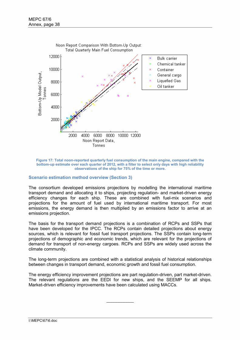
MEPC 67/6 Annex, page 38
I:\MEPC\67\6.doc
Figure 17: Total noon-reported quarterly fuel consumption of the main engine, compared with the bottom-up estimate over each quarter of 2012, with a filter to select only days with high reliability
observations of the ship for 75% of the time or more.
Scenario estimation method overview (Section 3) The consortium developed emissions projections by modelling the international maritime transport demand and allocating it to ships, projecting regulation- and market-driven energy efficiency changes for each ship. These are combined with fuel-mix scenarios and projections for the amount of fuel used by international maritime transport. For most emissions, the energy demand is then multiplied by an emissions factor to arrive at an emissions projection. The basis for the transport demand projections is a combination of RCPs and SSPs that have been developed for the IPCC. The RCPs contain detailed projections about energy sources, which is relevant for fossil fuel transport projections. The SSPs contain long-term projections of demographic and economic trends, which are relevant for the projections of demand for transport of non-energy cargoes. RCPs and SSPs are widely used across the climate community. The long-term projections are combined with a statistical analysis of historical relationships between changes in transport demand, economic growth and fossil fuel consumption. The energy efficiency improvement projections are part regulation-driven, part market-driven. The relevant regulations are the EEDI for new ships, and the SEEMP for all ships. Market-driven efficiency improvements have been calculated using MACCs.
___________


