Marika Karanassou, Hector Sala and Dennis J. Snower€¦ · Unemployment in the European Union: A...

Department of EconomicsUnemployment in the European Union: A Dynamic Reappraisal

Marika Karanassou, Hector Sala and Dennis J. Snower

Working Paper No. 480 December 2002 ISSN 1473-0278

Unemployment in the European Union: ADynamic Reappraisal

Marika Karanassou∗, Hector Sala�, and Dennis Snower�

August 2002

Abstract

This paper examines the movements in EU unemployment from twoperspectives: (a) the NRU/NAIRU perspective, in which unemploymentmovements are attributed largely to changes in the long-run equilibriumunemployment rate and (b) the chain-reaction perspective, in which unem-ployment movements are viewed as the outcome of the interplay between la-bor market shocks and prolonged lagged adjustment processes. We presentan empirical analysis that distinguishes between unemployment movementsarising from long-run equilibrium changes and those arising from laggedintertemporal adjustments. This analysis has far-reaching policy implica-tions. Our analysis shows that the rise in EU unemployment over the 1970sand Þrst part of the 1980s was due largely to permanent shocks (especiallythe rise in working-age population and the decline in capital formation),whereas the unemployment increase in the Þrst part of the 1990s was duelargely to temporary shocks (especially the fall in competitiveness and therise in real interest rates).KeyWords: Unemployment, natural rate, NAIRU, labor market shocks,

employment, labor force participation, wage determination, intertemporaladjustments, homogeneous dynamic panels, panel unit root tests.JEL ClassiÞcation Numbers: J32, J60, J64, E30, E37Acknowledgements: We gratefully acknowledge the Þnancial support

from the following sources: for all authors, IZA, Bonn, for the project on�Reappraising Europe�s Unemployment Problem�; for Marika Karanassou,the ESRC Grant No.R000239139; and for Hector Sala, the Fundacion BancoHerrero.

∗Department of Economics, Queen Mary, University of London, Mile End Road, London E14NS, UK; tel.: 020 7882-5090; email: [email protected]

�Department d�Economia Aplicada, Universitat Autònoma de Barcelona, 08193 Bellaterra,Spain; tel: ++ 34 93 581.11.53; email: [email protected]

�Department of Economics, Birkbeck College, University of London, 7 Gresse Street, LondonW1T 1LL, UK; tel: 020 7631-6408; email: [email protected]

1. Introduction

There are two fundamentally different economic views of unemployment: (i) Inthe frictionless equilibrium view, labor markets adjust quickly to external shocks(such as shocks to productivity, oil prices, or interest rates) and thus these marketsspend most of the time at or near their long-term equilibrium positions. Thus thelong-term equilibrium unemployment rate - at which there is no tendency for theparticipants to change their behavior, given the exogenous variables they face ineach period of time - is a good approximation of the actual unemployment rate.(ii) In the prolonged adjustment view, labor markets adjust only slowly to externalshocks, on account of adjustment costs. Consequently, the actual unemploymentrate can be away - possibly far away - from its long-term equilibrium for substantialtime spans.Naturally, these two views are not mutually exclusive. On the contrary, most

economists view them as polar extremes, and believe that labor market activityin practice lies in the interior of a spectrum between these extremes. Where,however, on this spectrum we Þnd ourselves turns out to be a matter of consid-erable importance, not only for our conceptual understanding of unemploymentmovements, but also for predictive and policy purposes.The theories of the �natural rate of unemployment� (NRU) or �non-accelerating

inßation rate of unemployment� (NAIRU) generally lie closer to the frictionlessequilibrium view than the prolonged adjustment view. These theories usually im-ply that European unemployment has tended to increase, from one recession tothe next over the past three decades, because the long-run equilibrium unemploy-ment has increased. These long-run changes have been ascribed to a variety offactors, such as generosity and duration of unemployment beneÞts, tax increases,interest rate increases, changes in the terms of trade, unionization, demographicfactors, and so on. The NRU and NAIRU theories do allow some adjustmentdynamics, but these transition effects are generally assumed to work themselvesout in the course of a short period - say, one or two years - and thus they cannotbe responsible for the long-climb in European unemployment from one businesscycle to the next.The �chain reaction theory of unemployment�, on the other hand, is an ex-

pression of the prolonged adjustment view. This theory views the movementsof European unemployment as the outcome of the interplay between a series oflabor market shocks and prolonged adjustments to these shocks. In this context,each labor market shock has a chain reaction of unemployment effects, extendingthrough time.1 The chain reactions arise from interactions among different (often

1The theory - described, for example, in Karanassou and Snower (1997, 1998) and Henry,Karanassou and Snower (2000) - derives its initial inspiration from the large literature on un-

2

complementary) lagged adjustment processes, as well as interactions between thedynamic structure of the shocks and the adjustment processes system.Permanent labor market shocks generally shift the long-run unemployment

equilibrium, as well as generate a chain reaction of intertemporal unemploymenteffects. The speedier is the intertemporal adjustment process, the faster willthe labor market approach its long-run equilibrium, and thus the greater theexplanatory power of the frictionless equilibrium approach. On the other hand,the longer it takes for the lagged adjustment mechanisms to work themselves out,the longer the labor market will be away from its long-run equilibrium in theaftermath of labor market shocks, and thus the greater the value-added of theprolonged adjustment approach.This paper examines unemployment in the European Union (EU) from these

two perspectives. We present an empirical analysis that distinguishes betweenunemployment movements arising from long-run equilibrium changes and thosemovements arising from lagged intertemporal adjustments.The adjustment dynamics to temporary and permanent labor market shocks

are quite different, as we will show. Thus, to conduct a careful empirical analysisof lagged adjustments, we need to divide the exogenous variables of our empiri-cal model into temporary components (TCs) and permanent components(PCs), whose changes are the temporary and permanent shocks.On this basis, we decompose the European unemployment trajectory into

� �temporary unemployment repercussions� (T ) which constitute theunemployment trajectory resulting from the TCs, and

� �permanent unemployment repercussions� (P) which comprise theunemployment trajectory generated by the PCs.

The temporary and permanent repercussions may, in turn, be divided into (a)the long-run unemployment effects of the TCs and PCs, which we denoteby uLRt (TC) and uLRt (PC) and (b) the dynamic adjustments toward theselong-run effects.Let us deÞne the frictionless equilibrium unemployment rate (FEU), at time t,

as that unemployment rate at which there is no tendency for the unemploymentrate to change (at time t), given the values of the exogenous variables (at time t) inthe underlying labor market model. In other words, the FEU is the unemploymentrate that would obtain once all the lagged adjustment processes have workedthemselves out, period by period, given the exogenous variables. Thus the FEUcan be identiÞed as the sum of the long-run unemployment effects of the temporary

employment persistence and hysteresis (e.g. Blanchard and Summers (1986) and Lindbeck andSnower (1987)).

3

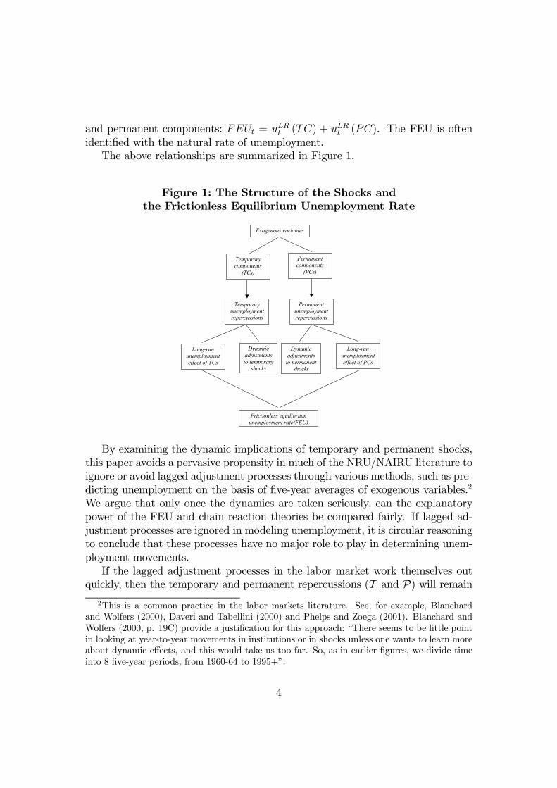
and permanent components: FEUt = uLRt (TC) + uLRt (PC). The FEU is oftenidentiÞed with the natural rate of unemployment.The above relationships are summarized in Figure 1.

Figure 1: The Structure of the Shocks andthe Frictionless Equilibrium Unemployment Rate

Exogenous variables

Temporary components

(TCs)

Permanent components

(PCs)

Temporary unemployment repercussions

Permanent unemployment repercussions

Long-run unemployment effect of TCs

Long-run unemployment effect of PCs

Dynamic adjustments to temporary

shocks

Dynamic adjustments

to permanent shocks

Frictionless equilibrium unemployment rate(FEU)

By examining the dynamic implications of temporary and permanent shocks,this paper avoids a pervasive propensity in much of the NRU/NAIRU literature toignore or avoid lagged adjustment processes through various methods, such as pre-dicting unemployment on the basis of Þve-year averages of exogenous variables.2

We argue that only once the dynamics are taken seriously, can the explanatorypower of the FEU and chain reaction theories be compared fairly. If lagged ad-justment processes are ignored in modeling unemployment, it is circular reasoningto conclude that these processes have no major role to play in determining unem-ployment movements.If the lagged adjustment processes in the labor market work themselves out

quickly, then the temporary and permanent repercussions (T and P) will remain2This is a common practice in the labor markets literature. See, for example, Blanchard

and Wolfers (2000), Daveri and Tabellini (2000) and Phelps and Zoega (2001). Blanchard andWolfers (2000, p. 19C) provide a justiÞcation for this approach: �There seems to be little pointin looking at year-to-year movements in institutions or in shocks unless one wants to learn moreabout dynamic effects, and this would take us too far. So, as in earlier Þgures, we divide timeinto 8 Þve-year periods, from 1960-64 to 1995+�.

4

close to the long-run unemployment effects of the temporary and permanent com-ponents (uLRt (TC) and uLRt (PC)), respectively, and thus the sum of the tem-porary and permanent repercussions (T + P)will follow the FEU (uLRt (TC) +uLRt (PC)) closely. However, if the lagged adjustment processes are lengthy, thenthe sum of the temporary and permanent repercussions may not track the FEUclosely, since it may take a long time for the full effects of the temporary andpermanent shocks to work themselves out.This is the context in which we investigate the roles of the FEU theory ver-

sus the chain reaction theory in explaining EU unemployment movements. Ourempirical analysis shows that adverse permanent shocks - particularly a rise inworking-age population and a decline in capital formation accompanying the pro-ductivity slow-down - played a major role in accounting for the rise in Europeanunemployment over the 1970s and Þrst half of the 1980s; but adverse temporaryshocks - particularly falling competitiveness, a rise in the real interest rate, andfurther temporary shocks associated with capital formation - were important inexplaining the unemployment increase in the Þrst half of the 1990s. Furthermore,our analysis shows that lagged labor market adjustment processes played a veryimportant role in modifying the unemployment effects of the temporary and per-manent shocks. In particular, these adjustment processes prevented the full effectsof the adverse permanent shocks from manifesting themselves right away; in fact,their inßuence was felt only gradually and progressively over the 1970s and Þrsthalf of the 1980s. Similarly, the favorable permanent shocks since then also haddelayed effects, contributing substantially to the recoveries in the late 1980s andlate 1990s. Finally, the adjustment processes played a substantial role in smooth-ing the inßuence of the temporary shocks and giving them persistent after-effectson unemployment. Our analysis suggests that the rise in EU unemployment inthe early 1990s can be attributed largely to this source.This investigation of the relative importance of long-run shifts versus lagged

adjustments has far-reaching policy implications. It is often observed that, overthe past three decades, the variations of European unemployment from one busi-ness cycle to the next (peak to peak, or trough to trough) have characteristicallybeen larger than the variations within each business cycle (peak to trough).3 Ifthese medium-term movements in European unemployment are attributed largelyto changes in the long-run labor market equilibrium, then policy makers shouldconcentrate on policies (such as changes in the duration and size of unemploymentbeneÞts or changes in interest rates) that inßuence this long-run equilibrium. Onthe other hand, if a signiÞcant share of the medium-term unemployment move-ments are attributed to intertemporal adjustments of European labor markets,then policy makers should also focus on measures (such as changes in job security

3See, for example, Layard, Nickell and Jackman (1991).

5

legislation to inßuence Þring costs, or job counselling measures to inßuence hir-ing costs) that affect the lagged adjustment processes and thereby improve labormarket more ßexibility in the aftermath of shocks.Even when these two approaches are concerned with the same policy mea-

sures, they focus attention on different attributes of these measures. For instance,changes in job security legislation (e.g. reductions in legislated Þring costs) may af-fect both the long-run equilibrium unemployment rate and the lagged adjustmentprocesses leading to that equilibrium. But whereas the effect of Þring costs onthe long-run unemployment equilibrium are generally ambiguous,4 the inßuenceof these costs on the lagged adjustment processes are usually quite predictable,e.g. a fall in Þring costs generally reduces employment inertia.On these accounts, how we interpret the medium-term movements in unem-

ployment is of far-reaching importance. Although questions of policy design lieoutside the scope of this paper, the potential policy implications provide an un-derlying motivation for our analysis.The paper is organized as follows. Section 2 summarizes the underlying con-

cepts and ideas. Section 3 presents the empirical model and discusses the relatedeconometric issues. Sections 4 describes our results. Section 5 relates our resultsto the standard single-equation analyses of unemployment. Section 6 concludes.

2. Underlying Concepts and Ideas

We estimate a structural vector autoregressive distributed lag model for the EUcountries:

A (L)yt = B (L)xt + εt, (2.1)

where L is the lag operator, yt is a vector of endogenous variables, xt is a vector ofexogenous variables (including deterministic trends), εt is a vector of identicallyindependently distributed error terms, A and B are coefficient matrices, and5

A (L) = A0 −A1L− ...−ApLp, B (L) = B0 +B1L+ ...+BqL

q.

4See, for example, Bentolila and Saint-Paul (1994), Bertola (1990), and Diaz and Snower(1996).

5The dynamic system (2.1) is stable if, for given values of the exogenous variables, all theroots of the determinantal equation

|A0 −A1L− ...−ApLp| = 0

lie outside the unit circle. Note that the estimated equations in Section 3 below satisfy thiscondition.

6

The endogenous variables of our system are employment (nt), the labor force(lt), the real wage (wt), and output (qt). All variables are national aggregates andall are in logarithms. Thus the equation system (2.1) consists of four equations:

1. the employment equation describes labor demand;

2. the labor force equation describes labor supply;

3. the wage equation indicates how real wages are determined (e.g. throughbargaining, efficiency wage considerations, union pressure, etc.);

4. the output equation is a production function; and

5. since all above variables are in logs, the unemployment rate (not in logs) is6

ut = lt − nt. (2.2)

Substituting the estimated equations (2.1) into (2.2), and further algebraicmanipulation, leads to the following Þtted �reduced form� unemployment rateequation:7

ut =IXj=1

φjut−j +JXj=0

θ0jxt−j , (2.3)

where the autoregressive parameters φ and the vectors θ of the coefficients of theexogenous variables are functions of the estimated structural parameters of (2.1).Next, we decompose the exogenous variables into their temporary and perma-

nent components: xt = vt+ zt, where vt is a vector of the temporary componentsand zt is a vector of the permanent components. (The nature of this decomposi-tion will be described in Section 4.) We thus obtain the following unemploymentequation:

ut =IXj=1

φjut−j +JXj=0

θ0jvt−j +JXj=0

θ0jzt−j. (2.4)

6Strictly speaking, this is an approximation.7The stability of the dynamic system (2.1) does not necessarily imply the stability of the

reduced form unemployment rate equation (2.2). For the stability of the latter we need all theroots of the polynomial

1− φ1L− ...− φILI = 0to lie outside the unit circle. Note that our estimations in Section 3 below satisfy this condition.

7

2.1. Unemployment Repercussions

In this context, the following unemployment effects may be identiÞed:

� the short-run unemployment effects of the temporary and permanent com-ponents: uSRt (TC) = θ00vt and u

SRt (PC) = θ00zt, respectively, and

� the long-run unemployment effects of the temporary and permanent com-ponents: uLRt (TC) =

³1−PI

j=1 φj

´−1PJj=0 θ

0jvt−j and

uLRt (PC) =³1−PI

j=1 φj

´−1PJj=0 θ

0jzt−j.

The temporary unemployment repercussions (the unemployment trajectoryresulting from the temporary components) are the contribution of the temporarycomponents to the unemployment through time:

Tt =IXj=1

φjTt−j +JXj=0

θ0jvt−j (2.5)

and the corresponding temporary shocks are ∆Tt.Similarly, the permanent repercussions are the unemployment contribution of

the permanent components through time:

Pt =IXj=1

φjPt−j +JXj=0

θ0jzt−j (2.6)

and the corresponding permanent shocks are ∆Pt.As equation (2.5) indicates, the temporary repercussion (Tt) in period t de-

pends on the temporary repercussions (Tt−j) in the previous I periods and onthe short-run unemployment effects of the temporary components (θ0jvt−j) in theprevious J periods. Suppose that our span of analysis (i.e. our sample period)is from t = 1 to t = T . Then, by the unemployment equation (2.4), the un-employment rate ut may be understood as the sum of three components: (i) thetemporary repercussions associated with the temporary components in the sampleperiod, (ii) the permanent repercussions associated with the permanent compo-nents in the sample period, and (iii) the temporary and permanent repercussions

8

associated with the temporary and permanent components that occurred beforethe sample period.8

Formally, let the temporary repercussions associated with the temporary com-ponents in the sample period be denoted by Tt |1≤t≤T . These within-sample tem-porary repercussions are given by equation (2.5), with the pre-sample values oftemporary repercussions (Tt−j) set equal to zero. Similarly, let the permanentrepercussions associated with the permanent components in the sample period bedenoted by Pt |1≤t≤T . These within-sample permanent repercussions are givenby the equation (2.6), with the pre-sample values of the permanent repercussions(Pt−j) set equal to zero. Finally, let the temporary and permanent repercussionsassociated with the temporary and permanent components that occurred prior tothe sample period be denoted by T Pt |t<1. Then the estimated unemploymentrate may be expressed as

ut = T Pt |t<1 +Tt |1≤t≤T +Pt |1≤t≤TIn empirical analysis, we can of course identify the three right-hand terms sep-

arately; what we cannot do identify separately are the temporary and permanentrepercussions that generate the the Þrst term (T P t |t<1), since we do not know theentire pre-sample history of the temporary and permanent components. Instead,we make a simple assumption. Since the temporary components are interprettedas transient shocks, we expect the lion�s share of the Þrst term to be generated bypermanent components. So, for simplicity, in the empirical analysis below we willassume that the entire Þrst term can be attributed to permanent components, sothat this term may be interpretted as part of the permanent repercussions.

8To see this straightforwardly, consider the simple case where the unemployment rate equa-tion (2.4) is of Þrst order and there is only one temporary component and one permanentcomponent:

ut = φut−1 + θzt + θvt, t = 1, 2, ..., T.

Using backward substitution, we can express the unemployment rate in terms of its pre-samplevalue u0 :

ut = φtu0 + θ

j=t−1Xj=0

φjzt + θ

j=t−1Xj=0

φjvt.

Here the Þrst right-side term stands for the temporary and permanent repercussions associatedwith the temporary and permanent components occurring before the sample period (embodiedin the initial unemployment rate u0); the second term stands for the permanent repercussionsassociated with the permanent components in the sample period; and the third term stands forthe temporary repercussions associated with the temporary components in the sample period.

9

2.2. The Frictionless Equilibrium Unemployment Rate

The frictionless equilibrium unemployment rate is the value that the unemploy-ment rate would achieve once all the lagged adjustment processes have workedthemselves out, given the exogenous variables. Thus the FEU is the sum of thelong-run unemployment effects of the temporary and permanent components:

FEUt ≡ uLRt (TC) + uLRt (PC) =³1−

XI

j=1φj

´−1Ã JXj=0

θ0jvt−j +JXj=0

θ0jzt−j

!.

(2.7)

As noted, the more quickly the lagged adjustment processes work themselvesout, the closer the temporary repercussions approximate the long-run unemploy-ment effects of the TCs and the closer the permanent repercussions approximatethe long-run unemployment effects of the PCs. Consequently, the closer the es-timated unemployment rates come to the frictionless equilibrium unemploymentrates through time.

2.3. A Simple Example

Suppose, for simplicity, that the unemployment equation is a Þrst-order autore-gression with one temporary component, vt, and one permanent component, zt:

ut = φut−1 + θxt = φut−1 + θvt + θzt, (2.8)

where 0 < φ < 1. This equation, in period t = 0, is illustrated by the unemploy-ment dynamics line UD0 in Figure 2.Consider the sequence of unemployment responses associated with a change in

the temporary component, viz., a single one-off unit shock in the form of a unit riseat period t: vt = 1. Thus the short-run (immediate impact) unemployment effectis Tt = θ, as illustrated in Figure 2 by the rise in the unemployment dynamicsline from UD0 to UD1 and the corresponding movement of the unemploymentequilibrium point from E0 to E1. Since the shock is temporary, it disappears afterperiod t: vt+j = 0, j ≥ 1. Thus the unemployment dynamics line in Figure 2returns to UD0 for t > 1.

10

Figure 2: Effects of Temporary and Permanent Shocks

E'E4

E3E2

E1

E0

ut

ut+1 450

UD0

UD1

Nevertheless, the unemployment effects of the temporary shock persist throughtime. In period t+1 the unemployment equilibrium point shifts to E2 in the Þgure,so that the change in the temporary unemployment repercussion in period t+1 isTt+1 = φθ. Next, in period t+2 the unemployment equilibrium point moves on toE3, and the corresponding change in the temporary unemployment repercussionis Tt+2 = φ2θ, and so on. Thus the entire sequence of unemployment changesresulting from the temporary shock, from period t+1 onwards, is Tt+j = φjθ, j ≥1.The unemployment repercussions associated with a permanent shock are quite

different. Let the shock be a permanent unit rise, beginning in period t: zt+j =1, j ≥ 0. Now the unemployment dynamics line moves from UD0 to UD1, asshown in Figure 2, and remains there forever. The short-run (immediate impact)unemployment effect is Pt = θ, as the unemployment equilibrium moves frompoint E0 to E1. In the following period, the equilibrium point moves to E4, andthe associated unemployment response to the permanent shock can be expressed asPt+1 ≡ θ+θφ, i.e. the sum of the effects of the permanent shock on unemploymentin periods t and t+1. As this process continues through time, the unemploymentrate gradually approaches its new equilibrium point E0. The unemployment effectof a unitary permanent shock k periods after its occurrence is Pt+k ≡ θ

Pkj=0 φ

j .This simple example shows why it is so important to distinguish between the

unemployment effects of the temporary and permanent components. The greaterthe persistence parameter φ (i.e. the steeper the unemployment dynamics line),the more persistent are the after-effects of the temporary shock, but the longer

11

it takes for the full (long-run) effects of the permanent shock to manifest them-selves. It can be shown, however, that this positive relation between the degreeof persistence from temporary shocks and the degree of inertia from permanentshocks does not hold invariably for higher-order unemployment autoregressions.In general, more persistence may be associated with more inertia or more over-shooting (the opposite of inertia), depending on the values of the autoregressiveparameters. So temporary and permanent shocks have quite different dynamicimplications and thus need to be studied separately.It is on this account that we decompose the time series of the exogenous vari-

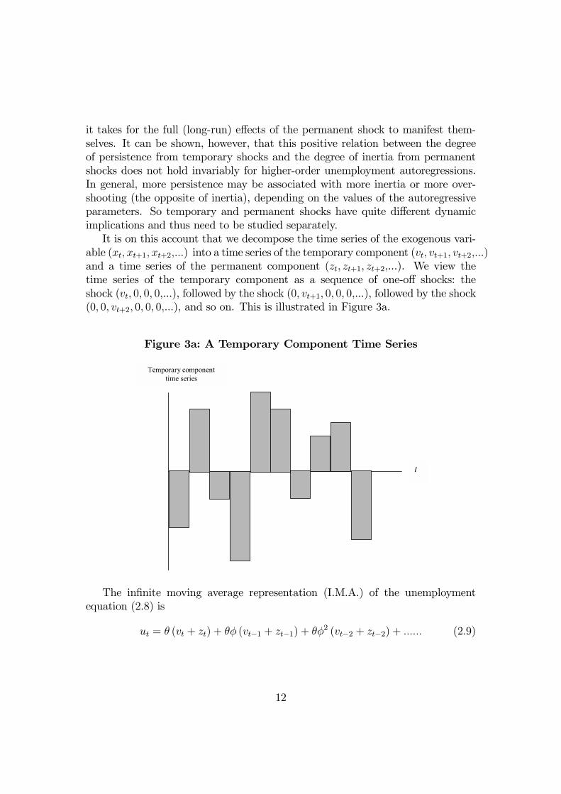
able (xt, xt+1, xt+2,...) into a time series of the temporary component (vt, vt+1, vt+2,...)and a time series of the permanent component (zt, zt+1, zt+2,...). We view thetime series of the temporary component as a sequence of one-off shocks: theshock (vt, 0, 0, 0,...), followed by the shock (0, vt+1, 0, 0, 0,...), followed by the shock(0, 0, vt+2, 0, 0, 0,...), and so on. This is illustrated in Figure 3a.

Figure 3a: A Temporary Component Time Series

t

Temporary component time series

The inÞnite moving average representation (I.M.A.) of the unemploymentequation (2.8) is

ut = θ (vt + zt) + θφ (vt−1 + zt−1) + θφ2 (vt−2 + zt−2) + ...... (2.9)

12

Thus the temporary unemployment repercussions (Tt+k) through time are givenby

Tt = θvt,Tt+1 = θvt+1 + θφvt,Tt+2 = θvt+2 + θφvt+1 + θφ2vt,

Tt+k = θkXj=0

φjvt+k−j. (2.10)

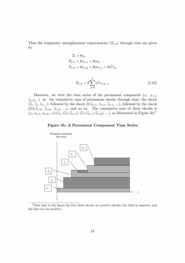
Moreover, we view the time series of the permanent component (zt, zt+1,zt+2,...) as the cumulative sum of permanent shocks through time: the shock(ezt, ezt, ezt,...), followed by the shock (0,ezt+1, ezt+1, ezt+1, ...), followed by the shock(0,0,ezt+2, ezt+2, ezt+2, ...), and so on. The cumulative sum of these shocks is(zt, zt+1, zt+2,...)=(ezt, (ezt+ezt+1), (ezt+ezt+1+ezt+2), ...), as illustrated in Figure 3b.9

Figure 3b: A Permanent Component Time Series

t

Permanent component time series

z1

2z�

3z�

4z�

5z�

6z�

9Note that in the Þgure the Þrst three shocks are positive shocks, the third is negative, andthe last two are positive.

13

Thus, the permanent repercussions (the unemployment trajectory resultingfrom the permanent components) are given by

Pt = (θezt) ,Pt+1 = θezt + θezt+1 + θφezt = (θezt + θφezt) + [θezt+1] ,Pt+2 = θezt + θezt+1 + θezt+2 + θφezt + θφezt+1 + θφ2ezt

=¡θezt + θφezt + θφ2ezt¢+ [θezt+1 + θφezt+1] + θezt+2,

and so on.10 In short, the permanent component11 at time t + k is Pt+k =θPk

j=0 φjzt+k−j .

3. The Empirical Model and Econometric Issues

We have estimated a panel data model for the EU countries covering the lastthree decades. This model has two features that differentiate it from the standardones used in pooled estimation: (i) it is a structural model, rather than merely astandard reduced-form equation and (ii) it is dynamic, rather than static.In this section we Þrst examine the appropriate methodology for such dynamic

panel data estimation, and then describe the results of our estimation.

3.1. Dynamic Panels

The advantages of using panel data sets for economic research are numerous andwell documented in the literature.12 For example, the pooling of observations ona cross section of countries over several time periods can increase the efficiency ofeconometric estimates and can provide a better understanding of the adjustmentmechanisms in dynamic relationships. In recent years, dynamic panel data andnonstationary panel time series models have attracted a lot of attention. As aresult, the study of the asymptotics of macro panels with large N (number ofunits, e.g. countries) and large T (length of the time series) has become the focusof panel data econometrics. Banerjee (1999) and Baltagi and Kao (2000), andSmith (2000) provide an overview of the above topics and survey the developmentsin this technical and rapidly growing literature.

10Observe that the terms in parentheses in the above equations show the unemployment effectsat each point in time of the permanent shock that occurs at period t. Similarly, the terms insquare brackets are the unemployment responses to the permanent shock that occurs at periodt+ 1.11The reason that we do not refer to initial values in this illustration is because we assume

that we can observe the whole history of exogenous variables.12See, for example, Hsiao (1986) and Baltagi (1995) for a detailed exposition of stationary

panel data estimation.

14

3.1.1. Panel Unit Root Tests

During the past several years testing for the order of integration in time serieshas been common practice in applied economic research. It is by now well knownthat the popular Dickey-Fuller (DF), augmented DF (ADF), and Phillips-Perron(PP) unit root tests have limited power in distinguishing the null of a unit rootfrom stationary alternatives with highly persistent deviations from equilibrium.Although testing for unit roots in panels is recent,13 it is generally accepted thatthe use of pooled cross-section time series data can generate more powerful unitroot tests.In our empirical work we employ the simple statistic proposed by Maddala

and Wu (1999) to test for panel unit roots. This is an exact nonparametric testbased on Fisher (1932):

λ = −2NXi=1

ln πi ∼ χ2 (2N) , (3.1)

where πi is the probability value of the ADF unit root test for the ith unit (coun-try). The Fisher test has several attractive features. First, since it combines thesigniÞcance of N different independent unit root statistics, it does not restrictthe autoregressive parameter to be homogeneous across i under the alternative ofstationarity. Second, the choice of the lag length and of the inclusion of a timetrend in the individual ADF regressions can be determined separately for eachcountry. Third, the sample sizes of the individual ADF tests can differ accordingto data availability for each cross-section. Finally, it should be noted that theFisher statistic can be used with any type of unit root test. Maddala and Wu(1999), using Monte Carlo simulations, conclude that the Fisher test outperformsboth the Levin and Lin (1993) and the Im et al (1997) tests14.

13See, for example, Levin and Lin (LL) (1993), Im, Pesaran and Shin (1997), Harris andTzavalis (1999), Maddala and Wu (1999). Note that the asymptotic properties of tests andestimators proposed for nonstationary panels depend on how N (the number of cross-sectionunits) and T (the length of the time series) tend to inÞnity, see Phillips and Moon (1999).14LL proposed asymptotic panel unit root tests which are based on pooled regressions. The

major criticism against the LL tests is that, under the alternative of stationarity, the autore-gressive coefficient is the same across all units (i.e. H1 : ρ1 = ρ2 = ... = ρN = ρ < 0).This restrictive assumption is relaxed in the asymptotic test proposed by Im, Pesaran and

Shin (IPS) (1997). Like the Fisher test, and in contrast to the LL tests, the IPS test is based onthe individual ADF regressions for each of the N cross-section units. While the Fisher test usesthe probability values of the individual ADF tests, the IPS uses their test statistics. Comparedto the Fisher test, the disadvantage of the IPS test is that it implicitly assumes the same T forall countries and the same lag length for all the individual ADF regressions.

15

3.1.2. Estimation of Dynamic Panels

We estimate the short-run and long-run parameters of behavioral relationships byusing dynamic panel data models, i.e. models characterized by the presence oflagged dependent variables among the regressors, such as15

yit = αyi,t−1 + β 0xit + εit, (3.2)

where α is a scalar, β is a K × 1 vector of constants, and xit is a K × 1 vectorof explanatory variables. The disturbances are assumed to follow a one-way errorcomponent model16

εit = µi + νit, i = 1, ...,N, t = 1, ..., T, (3.3)

where νit ∼ iid (0,σ2ν) with Cov (εit, εjt) = 0, for i 6= j. The scalar µi representsthe effects that are speciÞc to the ith unit and are assumed to remain constantover time. In this case, equations (3.2)-(3.3) give the Þxed-effects (FE) model:slope coefficients and variances are identical across groups and only intercepts areallowed to vary. Note that the FE estimator17 is the most common estimator fordynamic panels.In homogenous dynamic panels (i.e. models with constant slopes: αi = α,

and β 0i = β) the FE estimator is consistent as T → ∞, for Þxed N.18 However,pooling the data in dynamic heterogeneous panels (i.e. when αi 6= α, and β0i 6= β)leads to inconsistent estimators even for large N and T. This inconsistency19 wasdemonstrated by Pesaran and Smith (1995) (extended in Im, Pesaran and Smith(1996)) who advocated the use of group-mean estimators instead of pooled ones.The degree of heterogeneity is important in deciding whether to pool or not.

Given that the hypothesis of homogeneity will almost always be rejected20 whenthe sample size is sufficiently large and the signiÞcance level Þxed, Smith (2000)suggests to use a model selection criterion to decide on the poolability of the

15Although our estimations contain both the Þrst and second lags of the dependent variable,for expositional simplicity we ignore higher order lags in equation (3.2).16Again, we do not present the two-way error component model for expositional simplicity.

However, we used time-speciÞc effects (λt) in our estimations and for some of our structuralequations these appear in the form of a time trend.17The Þxed-effects estimator is also known as the least squares dummy variables (LSDV)

estimator, or the within-group or the analysis of covariance estimator.18Kiviet (1995) showed that the bias of the FE estimator in a dynamic model of panel data

has an approximation error of O¡N−1T−3/2

¢. Therefore, the FE estimator is consistent only

as T →∞, while it is biased and inconsistent when N is large and T is Þxed.19Robertson and Symons (1992) were the Þrst to notice the bias obtained when the true model

is static and heterogenous and the estimated one is dynamic and homogenous.20This is also noted by Baltagi and Griffin (1997): �...even though formal tests for homogeneity

are rejected as is the case here, like most researchers we proceed to estimate pooled models�.

16

data. We use the Schwarz Information Criterion (SIC) which penalizes over-parameterization more heavily than tests at the conventional signiÞcance levels.Baltagi and Griffin (1997) compare the performance of a large number of

homogenous and heterogeneous estimators in the context of dynamic demand forgasoline. The cross-section and time dimensions in the Baltagi and Griffin (BG)study are very similar to the dimensions of the panel data used in this paper: theyuse a panel data set for 18 OECD countries with annual data covering the period1960-1990. BG Þnd that the individual country estimates (both OLS and 2SLS)exhibit substantial variability, suggesting that �the individual country estimatesare highly unstable and unreliable,� and they Þnd that pooled estimators providemore plausible estimates. BG justify the use of pooled estimators by concludingthat �the efficiency gains from pooling appear to more than offset the biases dueto intercountry heterogeneities�.21

Given the above arguments by BG and the support for the homogeneity hy-pothesis by the Schwarz selection criterion (see the section below), we proceed byestimating our dynamic panel using the Þxed effects estimator.

3.2. The EU model

3.2.1. The Data

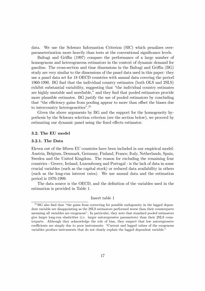
Eleven out of the Þfteen EU countries have been included in our empirical model:Austria, Belgium, Denmark, Germany, Finland, France, Italy, Netherlands, Spain,Sweden and the United Kingdom. The reason for excluding the remaining fourcountries - Greece, Ireland, Luxembourg and Portugal - is the lack of data in somecrucial variables (such as the capital stock) or reduced data availability in others(such as the long-run interest rates). We use annual data and the estimationperiod is 1970-1999.The data source is the OECD, and the deÞnition of the variables used in the

estimation is provided in Table 1.

Insert table 121BG also Þnd that �the gains from correcting for possible endogeneity in the lagged depen-

dent variable are disappointing as the 2SLS estimators performed worse than their counterpartsassuming all variables are exogenous�. In particular, they note that standard pooled estimatorsgive larger long-run elasticities (i.e. larger autoregressive parameters) than their 2SLS coun-terparts. Although they acknowledge the role of bias, they suspect that low autoregressivecoefficients are simply due to poor instruments: �Current and lagged values of the exogenousvariables produce instruments that do not closely explain the lagged dependent variable.�

17

3.2.2. Panel Unit Roots

We use the Fisher statistic (3.1) proposed by Maddala and Wu (1999) to test forpanel unit roots. As noted, the Fisher test is based on the ADF regressions for theindividual countries. The order of augmentation and the sample size are allowed tovary in the individual unit root tests, and a time trend is included when necessary.Table 2 reports the Fisher statistics for all the variables used in our structuralequations. The null hypothesis is that the time series has been generated by anI (1) stochastic process, and the test follows a chi-square distribution with 22degrees of freedom (the 5% critical value is approximately 34). Note that all thepanel unit root test statistics are greater than the critical value, so the null of aunit root can be rejected at the 5% signiÞcance level. Thus we can proceed withstationary panel data estimation techniques.

Insert table 2

3.2.3. The multi-equation system

As noted, our empirical model comprises four estimated equations - the employ-ment, labor supply, wage setting, and production equations - plus the deÞnitionof the unemployment rate.In the employment equation, labor demand depends negatively on the real

wage and the real interest rate, and positively both on the level and the growthrate of capital stock. Labor demand also depends positively on competitiveness(the ratio of the import price to the GDP deßator); this inßuence could operatethrough Þrms� costs of imported inputs.22

Insert table 3

The wage equation is also plausible, showing the real wage to depend negativelyon the unemployment rate and indirect taxes, and positively on productivity andsocial security beneÞts.

Insert table 4

In the labor supply equation, the size of the labor force depends negatively onthe level and growth of the unemployment rate (thereby exhibiting the commondiscouraged-worker effects) and positively on the working-age population. The

22Note that labor demand also depends positively on the time trend, which is meant to capturelabor-augmenting technological change.

18

long-run elasticity of labor supply with respect to the working-age population isrestricted to unity.23

Insert table 5

Finally, the estimated production function is standard, with output dependingpositively on employment, the capital stock, and a time trend.24

Insert table 6

It is important to point out an unconventional feature of this model. Althoughit is natural to let labor demand and labor supply depend on trended variablessuch as the capital stock and working-age population, the resulting system of es-timated equations implies a reduced-form unemployment equation in which theunemployment rate depends on these trended variables as well. Since the un-employment rate is untrended in practice (viz., it does not approach zero or 100percent with the passage of time), it follows that the long-run growth rates of thetrended variables must be such that the linear combination of these variables inthe reduced-form unemployment equation is untrended.Most conventional empirical labor market models, by contrast, are speciÞed in

such as way that in the resulting reduced-form unemployment equation, the long-run unemployment rate only depends on stationary variables.25 This approachreßects what may be call the �unemployment invariance hypothesis,� accordingto which the behavior of the labor market ensures that the long-run unemploy-ment is invariant with respect to the capital stock, productivity, the labor force,and other trended variables. The restrictions that this hypothesis imposes on em-pirical models are usually rejected by the data, but they are imposed nevertheless,with the common argument that the long-run unemployment rate, being station-ary, cannot depend on non-stationary variables. But this argument is not correct.It presupposes that the labor market, by itself, contains all the equilibrating mech-anisms that guarantee unemployment invariance. But all that is required is justthat all the markets in the general equilibrium system perform such equilibration.Accordingly, if the labor market does not perform ensure unemployment invari-ance on its own, but performs this function in conjunction with the other marketsin the economy, then it can be shown that the long-run unemployment rate will

23The Wald test could not reject this restriction at the conventional 5% signiÞcance level.Note also that the real wage has a weak contractionary inßuence on labor supply, suggesting aslightly dominant income effect.24The production function also captures the inßuence of raw materials via the oil price.25See, for example, Layard, Nickell, and Jackman (1991).

19

depend on non-stationary variables, but the long-run combination of these vari-ables appearing in the reduced-form unemployment equation is stationary. (Thisargument is made formally in Karanassou and Snower (2002).)In our estimated system of labor market equations, differences in labor market

behavior across countries was captured solely through Þxed effects, viz., onlydiffering constants in the estimated equations (but identical coefficients for theexogenous variables and the endogenous regressors). In fact, the Schwarz modelselection criterion prefers this Þxed-effect model above over heterogeneous modelscontaining individual country time series regressions.SpeciÞcally, we select between each of the pooled models presented in Tables

3-6 and the corresponding individual regressions by using the Schwarz InformationCriterion (SIC).26 We compute the model selection criteria as follows:

SICpooled =MLL− 0.5kpooled log (NT ) , (3.4)

SICindividual =11Xi=1

MLLi −N [0.5ki log (T )] , (3.5)

whereMLLpooled, MLLi denote the maximum log likelihoods of the pooled modeland the ith country time series regression, respectively; kpooled is the number ofparameters estimated in the Þxed effects model (i.e. number of explanatory vari-ables plus the 11 country speciÞc effects), and ki is the number of parametersestimated in the individual country time series regression (i.e. number of ex-planatory variables plus an intercept); N and T denote the number of countriesand estimation period, respectively.The above criteria are given in Table 7. The Þxed effects model is preferred for

all our four behavioral equations: labor demand, wage setting, labor force, andproduction function. This means that our stationary dynamic panel is homoge-nous and the Þxed effects estimator is consistent.

Insert table 7

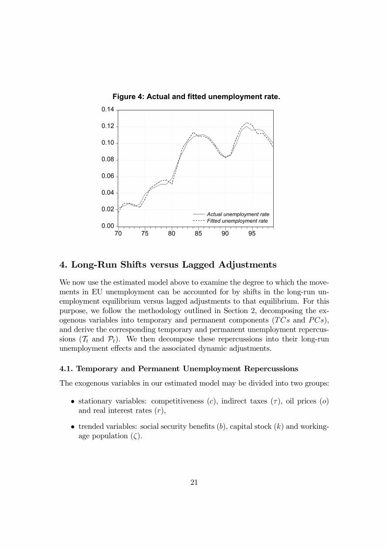
Despite this strong restriction of capturing cross-country differences only bythe constants in the estimated equations, our estimated system generates a Þttedunemployment rate that tracks the actual unemployment rate remarkably well.This is the case not only at the EU level, as shown in Figure 4, but also at thecountry-speciÞc level, as shown in Figures 5.

26The model that maximizes SIC is preferred.

20

0.00

0.02

0.04

0.06

0.08

0.10

0.12

0.14

70 75 80 85 90 95

Actual unemployment rateFitted unemployment rate

Figure 4: Actual and fitted unemployment rate.

4. Long-Run Shifts versus Lagged Adjustments

We now use the estimated model above to examine the degree to which the move-ments in EU unemployment can be accounted for by shifts in the long-run un-employment equilibrium versus lagged adjustments to that equilibrium. For thispurpose, we follow the methodology outlined in Section 2, decomposing the ex-ogenous variables into temporary and permanent components (TCs and PCs),and derive the corresponding temporary and permanent unemployment repercus-sions (Tt and Pt). We then decompose these repercussions into their long-rununemployment effects and the associated dynamic adjustments.

4.1. Temporary and Permanent Unemployment Repercussions

The exogenous variables in our estimated model may be divided into two groups:

� stationary variables: competitiveness (c), indirect taxes (τ), oil prices (o)and real interest rates (r),

� trended variables: social security beneÞts (b), capital stock (k) and working-age population (ζ).

21

0.00

0.02

0.04

0.06

0.08

70 72 74 76 78 80 82 84 86 88 90 92 94 96 98


Austria

0.00

0.02

0.04

0.06

0.08

0.10

0.12

0.14

0.16

70 72 74 76 78 80 82 84 86 88 90 92 94 96 98


Belgium

0.00

0.02

0.04

0.06

0.08

0.10

0.12

0.14

70 72 74 76 78 80 82 84 86 88 90 92 94 96 98


Denmark

0.00

0.02

0.04

0.06

0.08

0.10

0.12

70 72 74 76 78 80 82 84 86 88 90 92 94 96 98


Germany

0.00

0.05

0.10

0.15

0.20

70 72 74 76 78 80 82 84 86 88 90 92 94 96 98


Finland

0.00

0.02

0.04

0.06

0.08

0.10

0.12

0.14

70 72 74 76 78 80 82 84 86 88 90 92 94 96 98


France

0.00

0.02

0.04

0.06

0.08

0.10

0.12

0.14

70 72 74 76 78 80 82 84 86 88 90 92 94 96 98


Italy

0.00

0.02

0.04

0.06

0.08

0.10

0.12

0.14

70 75 80 85 90 95


Netherlands

0.00

0.05

0.10

0.15

0.20

0.25

0.30

70 72 74 76 78 80 82 84 86 88 90 92 94 96 98


Spain

0.00

0.02

0.04

0.06

0.08

0.10

0.12

70 72 74 76 78 80 82 84 86 88 90 92 94 96 98


Sweden

0.00

0.02

0.04

0.06

0.08

0.10

0.12

0.14

70 72 74 76 78 80 82 84 86 88 90 92 94 96 98


United Kingdom

Figure 5: Actual and fitted unemployment rates for individual EU countries

For the Þrst group of variables, the permanent components are identiÞed asthe sample means, leaving the temporary components as the random variations

22

around these means (i.e. the actual values of the variables minus the means).For the second group of variables, by contrast, the permanent components areidentiÞed as the Hodrick-Prescott Þltered series, and the temporary componentsare the variations around these series (i.e. the actual values of the variables minusthe Þltered series). These decompositions are simple, transparent and intuitivelyplausible.The simplest way of measuring the permanent components is through their

short-run unemployment effects, uSRt (PC). In this way, all the permanent com-ponents can be measured on a common scale, in a way immediately relevant tounemployment. These short-run (impact) effects are given in Figure 6. Withreference to the unemployment equation (2.4) (ut =

PIj=1 φjut−j+

PJj=0 θ

0jvt−j+PJ

j=0 θ0jzt−j), the short-run unemployment effect of the permanent components zt

(i.e. the inßuence of zt on ut, within the same period) is given by uSRt (PC) = θ00zt.The Þrst line (I) in Figure 6 denotes the constant plus the trend plus the per-manent components of the capital stock and the working-age population. Thesecond line (II) adds the permanent components of social security beneÞts to lineI; the third line (III) adds the permanent component of competitiveness to line II;and so on. Observe that each group of exogenous variables makes a signiÞcant,and comparably large contribution to the total short-run effects of the permanentcomponents.

0.00

0.04

0.08

0.12

0.16

70 72 74 76 78 80 82 84 86 88 90 92 94 96 98

Figure 6: Short-run unemployment effectsof the permanent components (PCs)

I = Cnst, Trend + PCs of capital stock and population

II = I + PCs of benefits

III = II + PCs of competitiveness

IV = III + PCs of indirect taxes

V = IV + PCs of oil price

VI = V + PCs of real interest rate

Along the same lines, the short-run unemployment effects of the temporarycomponents vt on ut are given by uSRt (TC) = θ00vt, and are presented in Figures7a and 7b.

23

-0.02

-0.01

0.00

0.01

0.02

70 72 74 76 78 80 82 84 86 88 90 92 94 96 98

I=TCs of capital stock and polulationII=II + TCs of benefitsIII=II + TCs of competitiveness

I, II

III

Figure 7a: Short-run unemployment effectsof the temporary components (TCs)

-0.02

-0.01

0.00

0.01

0.02

0.03

70 72 74 76 78 80 82 84 86 88 90 92 94 96 98

Figure 7b: Short-run unemployment effectsof the temporary components (TCs)

VI

III, IV, V

III=II + TCs of competitivenessIV=III + TCs of indirect taxesV=IV + TCs of oil priceVI=V + TCs of interest rate

The Þrst line (I) in the Þgure describes the temporary components of the capi-tal stock and the working-age population; the second line (II) adds the temporarycomponents of social security beneÞts to line I; and so on. It is important toobserve that only the capital stock and population, competitiveness, and the in-terest rate make a substantial contribution to the total short-run effect of theTCs. Hence, since the contribution of social security beneÞts is very small, andthus the lines I, II are almost identical (and indistinguishable to the naked eye inFig. 7a). Similarly, since the contributions of indirect taxes and the oil price issmall, lines III, IV, and V are also indistinguishable.As we have seen in Section 1, the unemployment impact effects of the tem-

porary and permanent components are followed by a chain reaction of laggedadjustments. We derive the temporary and permanent unemployment repercus-sions, given by equations (2.5) and (2.6), as the cumulation through time of thesechain reactions for each successive temporary and permanent component, respec-tively. SpeciÞcally, the temporary repercussions are derived by setting the per-manent components of the exogenous variables and the pre-sample values of theendogenous variables equal to zero, and simulating our estimated system with thetemporary components alone. To obtain the permanent repercussions, we set thetemporary components of the exogenous variables equal to zero, the pre-samplevalues of the endogenous variables equal to their actual values, and simulate thesystem with the permanent components alone.Figure 8 describes the temporary repercussions and then adds them to the

permanent repercussions. Observe that the sum of the temporary and permanentrepercussions (Tt+Pt) tracks the Þtted unemployment rate reasonably closely.2727As explained in Section 2.1., the temporary and permanent repercussions should add up to

the dynamic Þtted values of unemployment. This is indeed the case for each of the individualcountries in our panel. However, for our panel as a whole this decomposition is not feasible due

24

Observe that the permanent repercussions play the dominant role in explaining thesteep upward climb of EU unemployment in the 1970s and early 1980s, whereasthe temporary repercussions are dominant in the 1990s.

-0.02

0.00

0.02

0.04

0.06

0.08

0.10

0.12

0.14

70 75 80 85 90 95

Unemployment rate(dynamic fit)

Figure 8: Temporary and permanent repercussions.

Temporary repercussions

Temporary plus permanentrepercussions(dotted line)

It can be shown that the temporary repercussions account for 32 percent of thevariations in the actual unemployment rate, whereas the permanent repercussionsaccount for 50 percent. To obtain these statistics, we regress the temporaryrepercussions on the permanent ones and save the residuals. We then regressthe unemployment rate on this residual series. This gives R2 = 0.32. Similarly,when we regress the unemployment rate on the residuals of a regression of thepermanent repercussions on the temporary ones, we obtain R2 = 0.50. In short,32% is the portion of the unemployment variation explained by that part of thetemporary repercussions which is uncorrelated with the permanent repercussions.Similarly, 50% of total unemployment variation can be attributed to this part ofpermanent repercussions which is uncorrelated with the temporary repercussions.Whereas the sum of the individual contributions of the temporary and perma-

nent repercussions to explaining unemployment variation is 82%, the temporary

to the inherent nonlinearity in the deÞnition of the unemployment rate: The EU unemploymentrate is computed as the difference between the log of the EU labor force and the log of theEU employment level; this is not the same as the sum of the logs of the EU countries� laborforces minus the sum of the logs of the EU countries� employment. This accounts for thethe discrepancy between the dynamic Þtted values and the sum of temporary plus permanentcomponents in Figure 8.

25

and permanent repercussions can jointly explain 96% of the unemployment varia-tion (this is theR2obtained by regressing the unemployment rate on both series).28

4.2. Long-run Unemployment Effects and Lagged Adjustments

We now decompose the temporary and permanent repercussions into long-rununemployment effects and the associated lagged adjustments.We derive the long-run unemployment effects of the temporary components,

uLRt (TC), by setting permanent components equal to zero, setting the lag op-erators associated with all endogenous variables in our estimated system equalto unity, simulating the system, and deriving the associated unemployment timeseries. These uLRt (TC) effects are shown in Figure 9. Observe that they are muchmore volatile than the temporary repercussions (Tt), with the cyclical swings cor-responding to the major upturns and downturns in EU labor markets over thesample period: the recession of the mid-1970s following the Þrst oil-price shock,the rise in unemployment around 1978 due to reduced capital accumulation (whichwas, in turn, a lagged response to the previous recession), the recession of theearly 1980s following the second oil-price shock, the boom of the late 1980s, therecession of the early 1990s, and the boom of the late 1990s.

-0.1

0.0

0.1

0.2

70 75 80 85 90 95

Temporary repercussions

Long-run unemployment effects of TCs

Figure 9: Unemployment variations from temporary shocks.

The difference between the two series, Tt− uLRt (TC), are accounted for by thelagged adjustments to the temporary shocks. Clearly the lagged adjustment pro-cesses have played two important roles in modifying the unemployment inßuence

28Due to the correlation between the temporary and permanent repercussions, there is a partin the explained variation of unemployment which cannot be attributed to either of the twoseries because there is no obvious way to divide it between them.

26

of temporary shocks: (i) they are smoothed intertemporally and (ii) they are givenpersistent after-effects. For example, the large positive spikes in the uLRt (TC) inthe early 1980s and early 1990s is smoothed out, and the uLRt (TC) remains highfor about half a decade thereafter.Along the same lines, long-run unemployment effects of the permanent com-

ponents, uLRt (PC), are obtained by setting temporary components equal to zero,setting the lag operators associated with all endogenous variables in our esti-mated system equal to unity, simulating the system, and deriving the associatedunemployment time series. These effects are given in Figure 10. We identify thedynamic adjustments to the PCs as the difference between the permanent reper-cussions and the long-run unemployment effects of the permanent components.Observe that uLRt (PC) lies well above the permanent repercussions in the

Þrst part of the sample period, and this helps explain the steep rise of Europeanunemployment in the 1970s and Þrst part of the 1980s. Here the lagged adjustmentprocesses have played a major role in preventing the full effects of the permanentcomponents from manifesting themselves. Thus the high long-run unemploymenteffects in the 1970s and early 1980s leads only to a slow and steady rise of thepermanent repercussions.Observe, furthermore that, from the mid-1980s onwards, uLRt (PC) was slightly

below the permanent repercussions, leading to a gradual fall in the permanentrepercussions. On its own, this conÞguration would have led to a slow decline ofthe unemployment rate; but as it turned out, the bulge of temporary shocks inthe early 1990s sent EU unemployment upwards again.Why were the long-run unemployment effects of the permanent components so

high in the 1970s and early 1980s? The underlying data show that uLRt (PC) wasso high in the Þrst part of the 1970s because the labor supply increased markedlyin the late 1960s and early 1970s, as the postwar baby-boom generation enteredthe labor force. A major reason why uLRt (PC) remained so high throughoutthe 1970s was the productivity slow-down after the Þrst oil-price shock and theaccompanying drop in capital formation. In the late 1980s and 1990s, however,the working-age population grew less rapidly relative to the growth of the capitalstock, and thus uLRt (PC) fell gradually.

27

0.00

0.02

0.04

0.06

0.08

0.10

0.12

0.14

0.16

0.18

70 75 80 85 90 95

Figure 10: Unemployment variations from permanent shocks.

Long-run unemployment effects of the PCs

Permanentrepercussions

Figures 9 and 10 illustrate how dramatically the adjustment processes to tem-porary shocks differ from those to permanent shocks. This difference - temporaryshocks are smoothed and have persistent after-effects, whereas permanent shocksare kept from manifesting themselves fully - provides an empirical justiÞcation fordistinguishing between the temporary and permanent components. The Þguresalso show that both the temporary and permanent repercussions had importantroles to play in accounting for the movements in EU unemployment. The rise inEU unemployment over much of the 1970s and Þrst half of the 1980s largely followsthe permanent repercussions - particularly those associated with the movementsin the capital stock and working-age population. However, the rise in EU unem-ployment in the Þrst part of the 1990s is tracked by the temporary repercussions- particularly those associated with the movements in the interest rate and socialsecurity beneÞts.

4.3. The Frictionless Equilibrium Unemployment Rate

As noted, the FEU, or long-run unemployment rate uLRt , can be derived as thesum of the long-run unemployment effects of the temporary and permanent com-ponents. These are presented in Figure 11. The cyclical swings of the long-rununemployment rate of course follow the ups and down of the long-run unemploy-ment effects of the temporary components. Over the longer run, observe thatthere are two large bulges of the long-run unemployment rate. The Þrst - extend-ing from the mid-1970s to the mid-1980s - is due primarily to uLRt (PC), whereasthe second - covering the Þrst part of the 1990s - comes primarily from uLRt (TC).

28

0.00

0.05

0.10

0.15

0.20

0.25

0.30

70 72 74 76 78 80 82 84 86 88 90 92 94 96 98

Figure 11: Actual and long-run equilibrium rate ofunemployment.

Actualunemployment rate

Long-rununemployment rate

The long-run unemployment rate does not track the actual unemploymentclosely at all. Little of the variation in actual unemployment is accounted forby variations in the long-run unemployment rate: regressing the actual on thelong-run unemployment rate yields an R2 = 0.007. Like the uLRt (TC) series, thelong-run unemployment rate is far more volatile than the actual unemploymentrate. Our empirical model suggests that, in the absence of the lagged labor mar-ket adjustment processes, EU unemployment would have been far higher than itactually was in the recession periods and far lower than it was in the boom times.Note that the long-run unemployment rate provides some indication of the

direction in which EU unemployment is moving. For instance, when the long-runrate was above the actual rate in the second half of the 1970s and Þrst half of the1980s, EU unemployment tended upwards; and when the long-run rate was belowthe actual rate in the second half of the 1980s and the second half of the 1990s, EUunemployment tended downwards. Nevertheless, the lagged adjustments to theselong-run movements appear to have been very prolonged - so prolonged that thecorrelation of the actual and long-run unemployment rates is very small indeed.On all these accounts, our analysis suggests strongly that the lagged adjust-

ment processes have played an important role in determining the movements ofEU unemployment.

5. Single-Equation versus Multi-Equation Analysis

The above analysis of unemployment stands in stark contrast to the many con-ventional empirical analyses that are based on single-equation models of unem-

29

ployment. These models - whose structure may be summarized by equation(2.3), ut =

PIj=1 φjut−j +

PJj=0 θ

0jxt−j - may be understood as the reduced

form of an equation system such as the one above. In this context, a particu-larly common way of deriving the FEU or NRU is to set the lag operators inthis equation equal to unity, and obtaining the resulting unemployment rate,which is thus equivalent to the long-run unemployment rate of equation (2.7):

FEUt =³1−PI

j=1 φj

´−1 ³PJj=0 θ

0jxt−j

´. In this context, as noted, the FEU

is the equilibrium unemployment rate at which there is no tendency for the un-employment rate to change, given the values of the exogenous variables. In thissection, we explore the relation between our analysis and this conventional single-equation approach.

5.1. The Single-Equation Approach

To compare the two approaches, we Þnd the FEU by estimating a single unem-ployment equation of the above type, choosing the same set of exogenous variablesas those in our estimated system.

Insert Table 8

0.00

0.02

0.04

0.06

0.08

0.10

0.12

0.14

70 75 80 85 90 95

Actual unemployment rateFitted unemployment rateFEU

Figure 12: FEU, actual and fitted unemployment rates:Single-equation model

Table 8 presents two versions of the single-equation model, one using all theexogenous variables of our estimated system29 (Version 2) and the other - our pre-ferred one - using only those exogenous variables that are statistically signiÞcant29Note that in Version 2 all the exogenous variables are included and they are speciÞed in the

same way as in the estimated multi-equation system (e.g. the capital stock enters both through

30

(Version 1).30 In the mainstream literature, a variety of other exogenous vari-ables have of course also been used to explain unemployment.31 For our purposes,however, it suffices to focus on the exogenous variables used in our estimatedequation system, since the underlying difference between our approach and thestandard single-equation approach can be identiÞed quite simply in this context.(It is also worth noting that most of the mainstream contributions tend to ig-nore or minimize the role of unemployment dynamics - through such means asBlanchard-Wolfer�s method of taking 5-year averages of institutional variables -and thus it is not surprising that they Þnd that the NRU plays a major rolewhereas the dynamic unemployment adjustments play a minor one in accountingfor unemployment movements.)Figure 12 presents the resulting FEU, alongside the Þtted and actual unem-

ployment rates. Observe that this FEU - in marked contrast to the FEU associatedwith our estimated equation system above - closely follows the actual unemploy-ment rate. How is this discrepancy between the standard single-equation FEUand our multi-equation FEU to be rationalized?

5.2. Comparing the Two Approaches

For expositional simplicity, consider the following two alternative models for esti-mating unemployment:

� a single-equation model (S-E) that involves the direct estimation of a singleunemployment rate (u) equation, and

� a multi-equation model (M-E) that estimates labor force (l) and employ-ment (n) equations and then subtracts employment from the labor force32

to derive the unemployment rate equation, which we will call the reducedform unemployment equation.

To begin with, suppose that the regressors used in S-E are identical to thoseused in each of the equations in M-E. Then the two models may be expressed asfollows, with the S-E model as

u = X1δ1 +X2δ2 + εu, (5.1)

its level and its lagged difference).30Although the interest rate is marginally signiÞcant, it is retained in Version 1 since it permits

a better speciÞcation of the model.31For example, Blanchard and Wolfers (2000), Phelps (1994), and Phelps and Zoega (2001)

use wage-pressure variables such as union power, interest rates, asset prices, and institutionalvariables such as job security and the magnitude and duration of unemployment beneÞts.32Recall that since the variables are in logs, we can approximate the unemployment rate as

u = l − n.

31

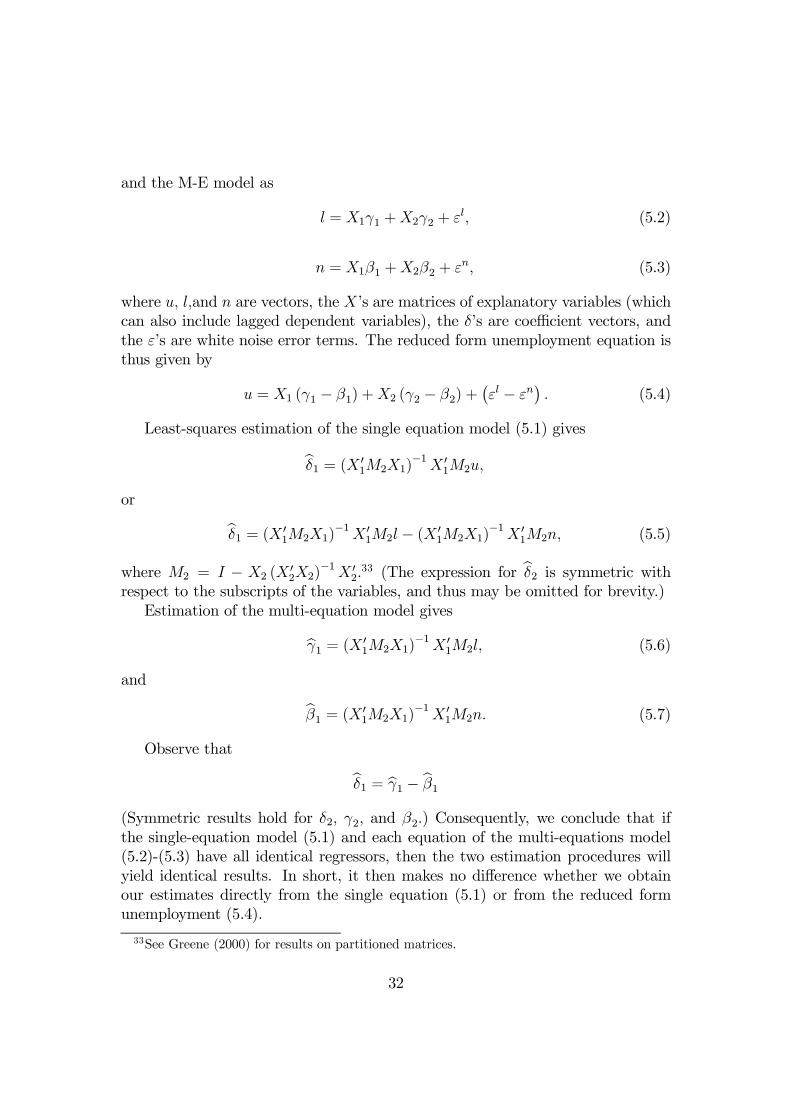
and the M-E model as

l = X1γ1 +X2γ2 + εl, (5.2)

n = X1β1 +X2β2 + εn, (5.3)

where u, l,and n are vectors, the X�s are matrices of explanatory variables (whichcan also include lagged dependent variables), the δ�s are coefficient vectors, andthe ε�s are white noise error terms. The reduced form unemployment equation isthus given by

u = X1 (γ1 − β1) +X2 (γ2 − β2) +¡εl − εn¢ . (5.4)

Least-squares estimation of the single equation model (5.1) gives

bδ1 = (X 01M2X1)

−1X 01M2u,

or

bδ1 = (X 01M2X1)

−1X 01M2l − (X 0

1M2X1)−1X 01M2n, (5.5)

where M2 = I − X2 (X 02X2)

−1X 02.33 (The expression for bδ2 is symmetric with

respect to the subscripts of the variables, and thus may be omitted for brevity.)Estimation of the multi-equation model gives

bγ1 = (X 01M2X1)

−1X 01M2l, (5.6)

and

bβ1 = (X 01M2X1)

−1X 01M2n. (5.7)

Observe that

bδ1 = bγ1 − bβ1(Symmetric results hold for δ2, γ2, and β2.) Consequently, we conclude that ifthe single-equation model (5.1) and each equation of the multi-equations model(5.2)-(5.3) have all identical regressors, then the two estimation procedures willyield identical results. In short, it then makes no difference whether we obtainour estimates directly from the single equation (5.1) or from the reduced formunemployment (5.4).

33See Greene (2000) for results on partitioned matrices.

32

Now, by contrast, suppose that the regressors used in the single-equation modelare not identical to the regressors used in each of the equations in the multi-equation model. For example, suppose that labor force and employment are givenby

l = X2γ2 + εl, (5.8)

n = X1β1 + εn, (5.9)

respectively. Then the reduced form unemployment equation is

u = X2γ2 −X1β1 +¡εl − εn¢ . (5.10)

In this case, clearly, the two estimated models produce quite different results.The Þtted values obtained from the previous reduced form unemployment equa-tion are

bu = (X 02X2)

−1X 02l − (X 0

1X1)−1X 01n, (5.11)

whereas the Þtted values of the single-equation model (5.1) are

bu = X1 (X 01M2X1)

−1X 01M2 (l − n) +X2 (X 0

2M1X2)−1X 02M1 (l − n) . (5.12)

In this context, there is an important empirical remark to be made, which en-ters the discussion surrounding the results obtained from single- or multi-equationmodels.Needless to say, when structural multi-equation systems are estimated, it is

generally not the case that each constituent equation has the same regressors.Thus it becomes impossible for the regressors of the S-E model to be identical toeach equation in the M-E model. Then the S-E model can no longer be viewedas an unbiased summary of the M-E model. Rather, the detailed economic inter-actions portrayed in the M-E model - including the dynamic interactions amongthe various lagged adjustment processes - can no longer be captured in the S-Emodel. In short, the single-equation model becomes misleading.34

34Of course, a similar aggregation problem arises when the M-E model above is comparedwith a more disaggregated M-E model. The problem is overcome once increasing disaggregationyields no further diversity of regressors in the component equations.

33

-0.04

-0.02

0.00

0.02

0.04

0.06

0.08

0.10

0.12

70 75 80 85 90 95

a. Temporary repercussions

Multi-equation model

Single-equation model

0.00

0.02

0.04

0.06

0.08

0.10

0.12

70 75 80 85 90 95

b. Permanent repercussions

Multi-equation model

Single-equation model

Figure 13: Unemployment repercussions in S-E and M-E models.

Consequently, it comes as no surprise that when the S-E model is used to derivethe temporary and permanent repercussions, the results are quite different fromthose of the M-E model above, as shown in Figures 13a and 13b. Observe that theS-E model gives temporary repercussions a misleadingly small role in explainingthe movements in EU unemployment: the temporary repercussions in the S-Emodel never account for as much as 2 percentage points of unemployment, andthe S-E model misses the 1990s bulge in temporary repercussions that is identiÞedby the M-E model. To compensate, the S-E model gives permanent repercussionsa misleadingly large role the upward drift of EU unemployment over the sampleperiod.Overall, the high level of aggregation inherent in single-equation models intro-

duces an interesting bias into the empirical analysis of unemployment movements:the role of the FEU (or NRU) is over-emphasized and, correspondingly, the roleof lagged adjustments is under-emphasized. As a comparison of Figures 11 and12 shows, the FEU tracks the actual unemployment rate closely in the S-E model(leaving little to be explained by dynamic adjustments) but not closely in theM-E model (leaving much more to be explained by dynamic adjustments). Thus,single-equation models are not a reliable way to evaluate the relative importanceof long-run shifts versus lagged adjustments in explaining the evolution of EUunemployment.

6. Conclusions

This paper has examined some important questions for the analysis of EU unem-ployment: Have the long swings and upward drift of European unemployment over

34

the past three decades been due primarily to changes in the underlying supply-and-demand relationships, causing shifts in the long-run equilibrium unemploy-ment rates? Or have lagged adjustments to these shifts played an even moreimportant role?In examining lagged adjustment dynamics, we have seen that there are striking

differences between the unemployment movements following temporary shocksand those following permanent shocks. Temporary shocks - such as changes inreal interest rates, competitiveness, oil prices, and taxes - may have persistentafter-effects on unemployment, whereas the long-run effects of permanent shocks- such as changes in the capital stock or working-age population - may take along time to manifest themselves (inertia) or there may be over-shooting. Onthis account, it is important to distinguish between temporary and permanentshocks in the analysis of unemployment dynamics. What has been the relativeimportance of temporary and permanent shocks in accounting for the movementsin EU unemployment?To address these questions, we have estimated a dynamic panel data model for

the EU countries over the last three decades. The model is an equation systemcomprising employment, wage, labor force and production equations, as well as adeÞnition of the unemployment rate. In this context, we derived the unemploy-ment repercussions of the temporary and permanent components of the exogenousvariables, and we decomposed these repercussions into long-run unemploymenteffects and dynamic adjustments. We found that the dynamic adjustments inresponse to the permanent shocks played a large role in accounting for rise ofEU unemployment in the 1970s and Þrst half of the 1980s, whereas the dynamicadjustments in response to the temporary shocks played a large role in explainingthe rise of EU unemployment in the early 1990s.In broad outline, this methodology suggests the following explanation of Euro-

pean unemployment movements. In the late 1960s and early 1970s, the Europeanlabor force increased rapidly as the postwar baby-boom generation became adultsand began looking for jobs. This large permanent shock took a long time to feedthrough European labor markets, leading to a steady rise in unemployment inthe 1970s. This inßuence was augmented by the productivity slow-down of themid-1970s that was accompanied by a downward shift in capital formation. Theafter-effects of these permanent changes, along with some temporary shocks - arise in interest rates and a fall in competitiveness - kept European unemploymentrising through the mid-1980s.The labor force shock reversed itself in 1980s and 1990s, as the labor supply

slowed down relative to the growth of the capital stock. This permanent shockalso took a long time to manifest itself, contributing to the fall in Europeanunemployment during the second half of the 1980s and the second half of the 1990s.

35

Meanwhile, in the early 1990s, high real interest rates and low competitiveness(i.e. a low ratio of import prices to GDP deßators, due in part to the surging USproductivity performance and other structural factors), were the temporary shocksthat sent European unemployment upwards during the Þrst part of the 1990s andit took some time before the unemployment rate came down signiÞcantly.This account of the European unemployment problem - in which lagged ad-

justment processes play a central role in describing unemployment movements - ishowever at odds with the story suggested by the standard single-equation models,which attribute much of the medium- and longer-run unemployment movementsto changes in the long-run unemployment equilibrium. We rationalize the discrep-ancy this approach and ours by showing that, on account of a dynamic aggregationproblem, single-equation unemployment models give a biased analysis of unem-ployment, over-emphasizing the role of long-run shifts and under-emphasizing therole of dynamic adjustments. We conclude that whereas there were substantialshifts in the long-run EU unemployment rate over the sample period, the pro-longed dynamic adjustments are indispensable in providing a balanced analysis ofEuropean unemployment.

36

References

[1] Baltagi, B. H. (1995): Econometric Analysis of Panel Data, NewYork: Wiley.

[2] Baltagi, B. H. and J. M. Griffin (1997): �Pooled estimators vs. their heteroge-neous counterparts in the context of dynamic demand for gasoline�, Journalof Econometrics, No. 77, 303-327.

[3] Baltagi, B. H. and C. Kao (2000): �Nonstationary Panels, Cointegration inPanels and Dynamic Panels: A Survey�, mimeo.

[4] Banerjee A. (1999): �Panel Data Unit Roots and Cointegration: AnOverview�, Oxford Bulletin of Economics and Statistics, special issue, 607-629.

[5] Bertola, G. (1990), �Job Security, Employment and Wages,� European Eco-nomic Review, 34, 851-86.

[6] Blanchard, O.J. and L. Summers (1986), �Hysteresis and the European Un-employment Problem,� NBER Macroeconomics Annual, vol. 1, Cambridge,Mass: MIT Press, 15-71.

[7] Blanchard, O.J. and J. Wolfers (2000): �The Role of Shocks and Institutionsin the Rise of European Unemployment: The Aggregate Evidence�, EconomicJournal, 110, March, C1-C33.

[8] Daveri, F. and G. Tabellini (2000): Unemployment, Growth and Taxation inIndustrial Countries�, Economic Policy, 0 (30), 47-88.

[9] Díaz, P., and D.J. Snower (1996), �Employment, Macroeconomic Fluctua-tions and Job Security,� CEPR Discussion Paper No. 1430.

[10] Fisher, R. A. (1932): Statistical Methods for Research Workers, Edinbutgh:Oliver & Boyd.

[11] Greene, W. (2000): Econometric Analysis, 4th Edition, New York: PrenticeHall.

[12] Harris, R. D. F. and E. Tzavalis (1999):�Inference for Unit Roots in DynamicPanels where the Time Dimension is Fixed�, Journal of Econometrics, 91,201-226.

[13] Henry, S.G.B., M. Karanassou, and D.J. Snower (2000), �Adjustment Dy-namics and the Natural Rate�, Oxford Economic Papers, 52, 178-203.

37

[14] Hsiao, C. (1986): Analysis of Panel Data, Cambridge: Cambridge UniversityPress.

[15] Im, K. S., Pesaran, M. H., and Y. Shin (1997): �Testing for Unit Roots inHeterogeneous Panels�, mimeo, Department of Applied Economics, Univer-sity of Cambridge.

[16] Im, K. S., Pesaran, M. H., and R. Smith (1996): Dynamic Linear Models forHeterogeneous Panels, p. 145-195 of Matyas and Sevestre.

[17] Karanassou, M., and D.J. Snower (1997), �Is the Natural Rate a ReferencePoint?�, 1997, European Economic Review, 41, 559-569.

[18] Karanassou, M., and D.J. Snower (1998), �How Labor Market FlexibilityAffects Unemployment: Long-Term Implications of the Chain Reaction The-ory�, 1998, Economic Journal, 108, May, 832-849.

[19] Karanassou, M., and D.J. Snower (2002), �Unemployment Invariance,�mimeo.

[20] Kiviet, J. F. (1995): �On bias, inconsistency, and efficiency of various esti-mators in dynamic panel data models�, Journal of Econometrics, 68, 53-78.

[21] Layard, P.R.J., Nickell, S.J. and R. Jackman (1991): Unemployment:Macroeconomic Performance and the Labor Market, Oxford: Oxford Uni-versity Press.

[22] Levin, A. and C. F. Lin (1993): �Unit Root Tests in Panel Data: NewResults�, Department of Economics, University of California at San Diego,Discussion Paper No. 93-56.

[23] Lindbeck, A., and D.J. Snower (1987), �Union Activity, Unemployment Per-sistence, and Wage-Employment Ratchets,� European Economic Review, 31,Feb., 157-167.

[24] Maddala, G. S. and S. Wu (1999): �A comparative Study of Unit Root Testswith Panel Data and a New Simple Test�, Oxford Bulletin of Economics andStatistics, special issue, 631-652.

[25] Pesaran, M.H. and R. Smith (1995): �Estimating long-run relationships fromdynamic heterogeneous panels�, Journal of Econometrics, 68, 79-113.

[26] Phelps, E. S. (1994): Structural Booms: The Modern Equilibrium Theory ofUnemployment, Interest and Assets, Harvard University Press, Cambridge(MA).

38

[27] Phelps, E. and G. Zoega (2001): �Structural booms: productivity expecta-tions and asset valuations,� Economic Policy, 32, April, 85-126.

[28] Phillips, P. C. B. and H. R. Moon (1999): �Linear Regression Limit Theoryfor Nonstationary Panel Data�, Econometrica, Vol. 67, No. 5, 1057-1111.

[29] Robertson, D. and J. Symons (1992): �Some Strange Properties of PanelData Estimators,� Journal of Applied Econometrics, 7, 175-189.

[30] Smith, R. P. (2000): �Estimation and inference with non-stationary paneltime-series data�, mimeo.

39

Table 1: DeÞnitions of variables.bt : real Social Security beneÞts per personct : competitiveness deÞned as log

¡ Import pricesGDP deßator

¢kt : real capital stocklt : labor forcent : employmentot : real oil pricesqt : real GDPrt : long-term real interest rates (%)t : time trendut : unemployment rate deÞned as ut = lt − ntwt : real compensation per person employedτ t : indirect taxes (as a % of GDP)θt : productivity deÞned as qt − ntζt : working-age populationNote: All variables in logs except otherwise speciÞed.Source: OECD.

Table 2: Panel Unit Root Tests.λ (nit) = 36.10λ (qit) = 42.88λ (kit) = 41.19λ (wit) = 159.79

λ (lit) = 35.12λ (rit) = 47.67λ (oit) = 42.67λ (cit) = 46.79

λ (ζ it) = 40.57λ (bit) = 91.45λ (τ it) = 46.24

Notes: λ (·) is the test proposed by Maddala and Wu (1999).The test follows a chi-square (22) distribution.The 5% critical value is approximately 34.

40

Table 3: Labor demand equation.Dependent variable: nt

Coefficient St. e. Prob.nt−1 1.42 0.039 0.000nt−2 −0.48 0.035 0.000wt −0.03 0.012 0.011kt 0.02 0.009 0.035∆kt 1.99 0.070 0.000∆kt−1 −1.65 0.093 0.000ct 0.02 0.006 0.003rt −0.001 0.000 0.019t 0.001 0.000 0.044

R2 0.999MLL 1108.9

Table 4: Wage equation.Dependent variable: wt

Coefficient St. e. Prob.wt−1 0.97 0.051 0.000wt−2 −0.14 0.045 0.002ut −0.29 0.045 0.000θt 0.50 0.056 0.000θt−1 −0.36 0.052 0.000bt 0.14 0.020 0.000bt−1 −0.12 0.022 0.000ot 0.005 0.002 0.020τ t −0.59 0.180 0.001τ t−1 0.41 0.189 0.030

R2 0.999MLL 912.0

41

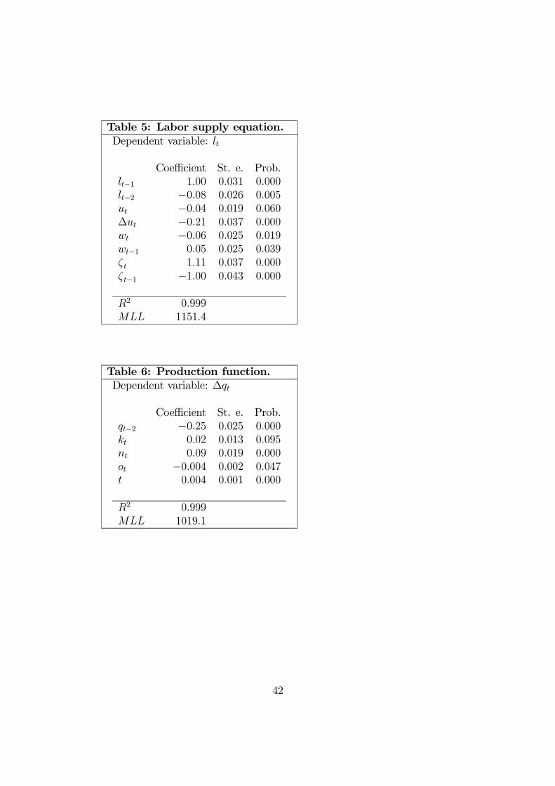
Table 5: Labor supply equation.Dependent variable: lt

Coefficient St. e. Prob.lt−1 1.00 0.031 0.000lt−2 −0.08 0.026 0.005ut −0.04 0.019 0.060∆ut −0.21 0.037 0.000wt −0.06 0.025 0.019wt−1 0.05 0.025 0.039ζt 1.11 0.037 0.000ζt−1 −1.00 0.043 0.000

R2 0.999MLL 1151.4

Table 6: Production function.Dependent variable: ∆qt

Coefficient St. e. Prob.qt−2 −0.25 0.025 0.000kt 0.02 0.013 0.095nt 0.09 0.019 0.000ot −0.004 0.002 0.047t 0.004 0.001 0.000

R2 0.999MLL 1019.1

42

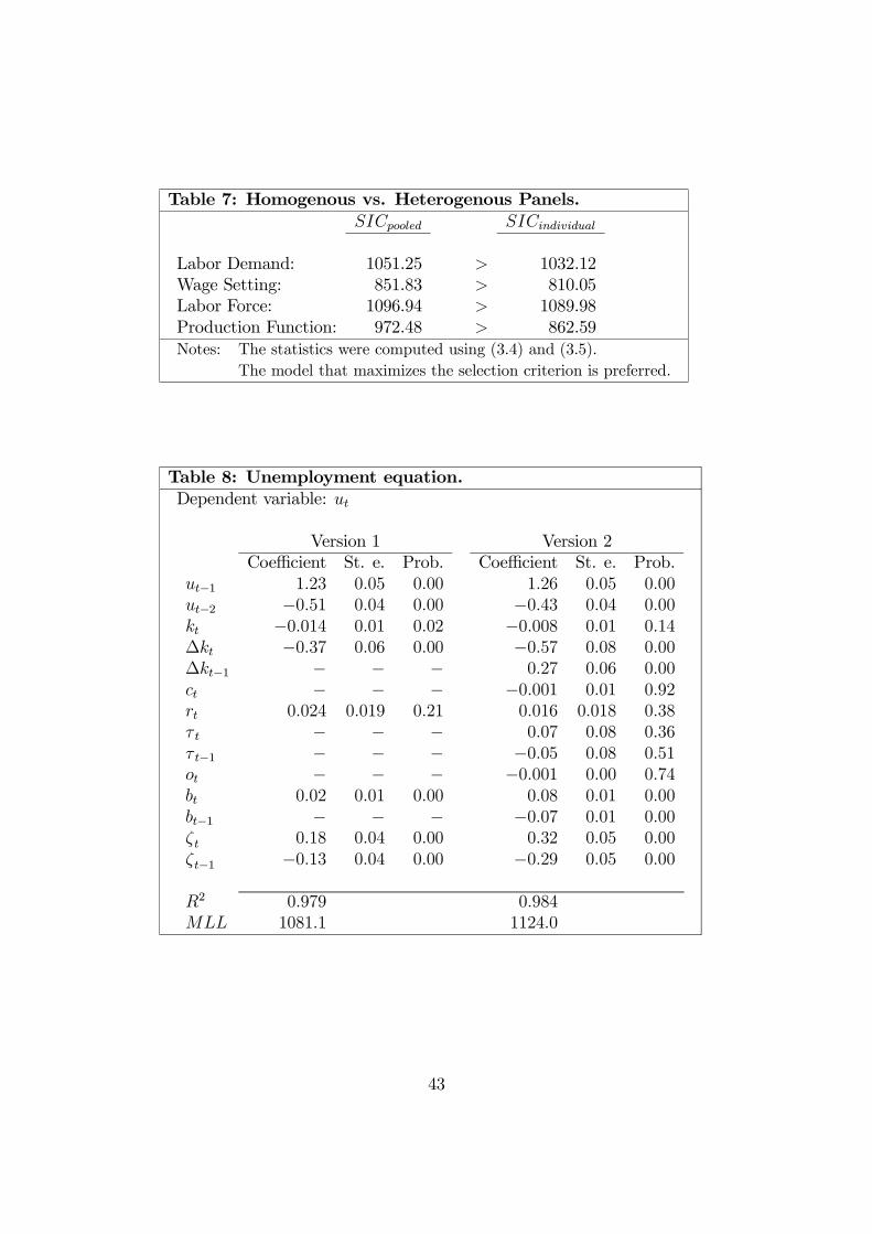
Table 7: Homogenous vs. Heterogenous Panels.SICpooled SICindividual

Labor Demand: 1051.25 > 1032.12Wage Setting: 851.83 > 810.05Labor Force: 1096.94 > 1089.98Production Function: 972.48 > 862.59Notes: The statistics were computed using (3.4) and (3.5).

The model that maximizes the selection criterion is preferred.

Table 8: Unemployment equation.Dependent variable: ut

Version 1 Version 2Coefficient St. e. Prob. Coefficient St. e. Prob.

ut−1 1.23 0.05 0.00 1.26 0.05 0.00ut−2 −0.51 0.04 0.00 −0.43 0.04 0.00kt −0.014 0.01 0.02 −0.008 0.01 0.14∆kt −0.37 0.06 0.00 −0.57 0.08 0.00∆kt−1 − − − 0.27 0.06 0.00ct − − − −0.001 0.01 0.92rt 0.024 0.019 0.21 0.016 0.018 0.38τ t − − − 0.07 0.08 0.36τ t−1 − − − −0.05 0.08 0.51ot − − − −0.001 0.00 0.74bt 0.02 0.01 0.00 0.08 0.01 0.00bt−1 − − − −0.07 0.01 0.00ζt 0.18 0.04 0.00 0.32 0.05 0.00ζt−1 −0.13 0.04 0.00 −0.29 0.05 0.00

R2 0.979 0.984MLL 1081.1 1124.0

43

This working paper has been produced bythe Department of Economics atQueen Mary, University of London

Copyright © 2002 Marika Karanassou, Hector Salaand Dennis J. Snower. All rights reserved.

Department of Economics Queen Mary, University of LondonMile End RoadLondon E1 4NSTel: +44 (0)20 7882 5096 or Fax: +44 (0)20 8983 3580Email: [email protected]: www.econ.qmul.ac.uk/papers/wp.htm

Marika Karanassou, Hector Sala and Dennis J. Snower€¦ · Unemployment in the European Union: A...

Documents

Transcript of Marika Karanassou, Hector Sala and Dennis J. Snower€¦ · Unemployment in the European Union: A...