Maryland Marcellus Shale Safe Drilling Initiative Study - Part 1
The Pennsylvania State University
The Graduate School
College of Agricultural Sciences
MARCELLUS SHALE NATURAL GAS DRILLING OPERATORS’
CHOICE OF WASTEWATER DISPOSAL METHOD
A Thesis in
Agricultural, Environmental, and Regional Economics
by
Caitlyn Edmundson
© 2012 Caitlyn Edmundson
Submitted in Partial Fulfillment of the Requirements
for the Degree of
Master of Science
December 2012
ii
The thesis of Caitlyn Edmundson was reviewed and approved* by the following:
Charles Abdalla
Professor of Agricultural and Environmental Economics
Thesis Adviser
James Dunn
Professor of Agricultural Economics
Brian Dempsey
Professor of Environmental Engineering
Richard Ready
Professor of Agricultural and Environmental Economics
Coordinator, Graduate Program in Agricultural, Environmental, and Regional Economics
*Signatures are on file in the Graduate School
iii
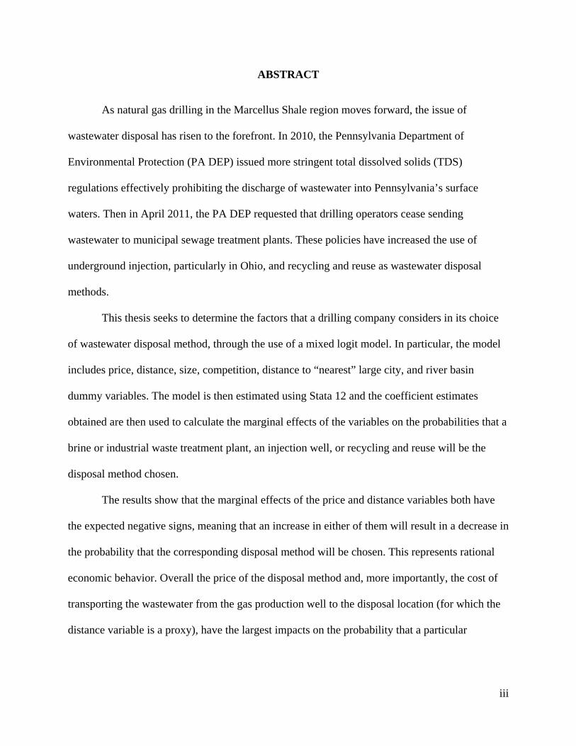
ABSTRACT
As natural gas drilling in the Marcellus Shale region moves forward, the issue of
wastewater disposal has risen to the forefront. In 2010, the Pennsylvania Department of
Environmental Protection (PA DEP) issued more stringent total dissolved solids (TDS)
regulations effectively prohibiting the discharge of wastewater into Pennsylvania’s surface
waters. Then in April 2011, the PA DEP requested that drilling operators cease sending
wastewater to municipal sewage treatment plants. These policies have increased the use of
underground injection, particularly in Ohio, and recycling and reuse as wastewater disposal
methods.
This thesis seeks to determine the factors that a drilling company considers in its choice
of wastewater disposal method, through the use of a mixed logit model. In particular, the model
includes price, distance, size, competition, distance to “nearest” large city, and river basin
dummy variables. The model is then estimated using Stata 12 and the coefficient estimates
obtained are then used to calculate the marginal effects of the variables on the probabilities that a
brine or industrial waste treatment plant, an injection well, or recycling and reuse will be the
disposal method chosen.
The results show that the marginal effects of the price and distance variables both have
the expected negative signs, meaning that an increase in either of them will result in a decrease in
the probability that the corresponding disposal method will be chosen. This represents rational
economic behavior. Overall the price of the disposal method and, more importantly, the cost of
transporting the wastewater from the gas production well to the disposal location (for which the
distance variable is a proxy), have the largest impacts on the probability that a particular
iv
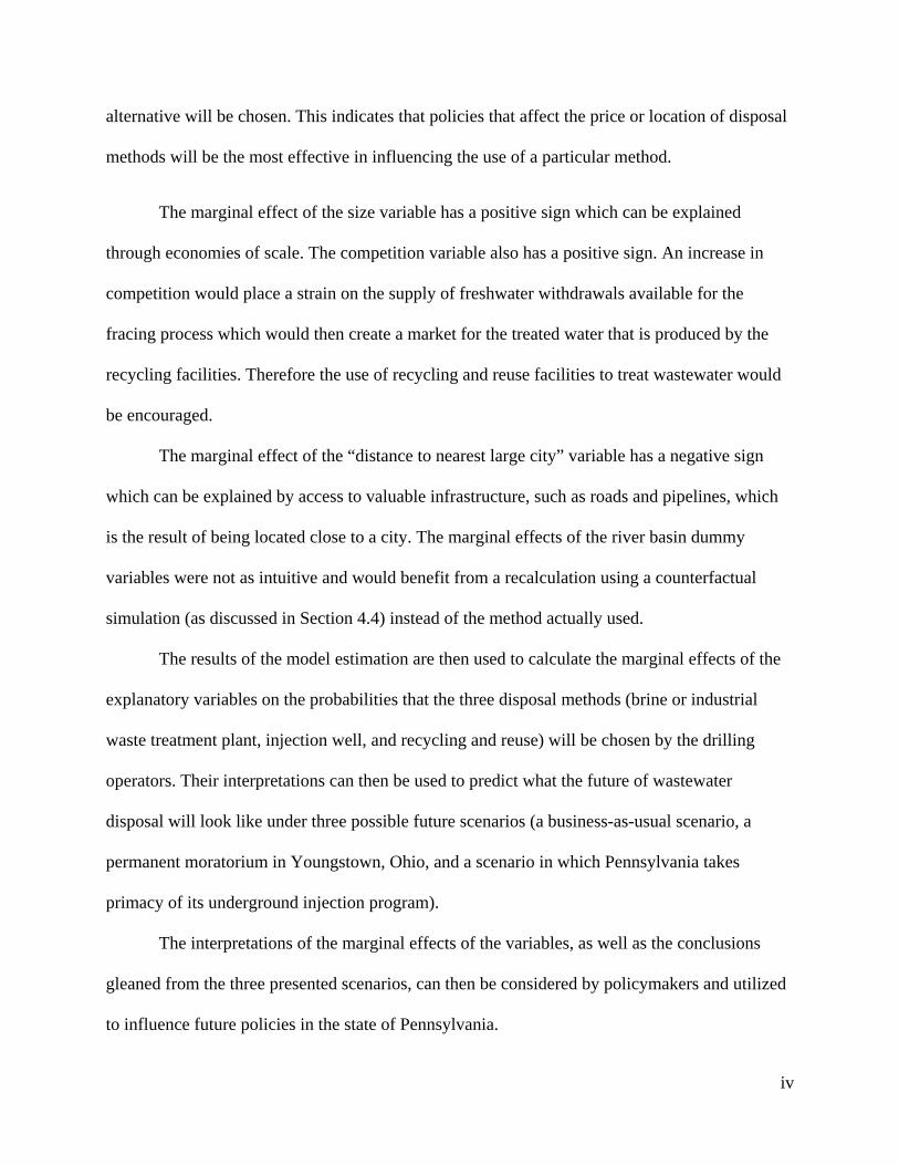
alternative will be chosen. This indicates that policies that affect the price or location of disposal
methods will be the most effective in influencing the use of a particular method.
The marginal effect of the size variable has a positive sign which can be explained
through economies of scale. The competition variable also has a positive sign. An increase in
competition would place a strain on the supply of freshwater withdrawals available for the
fracing process which would then create a market for the treated water that is produced by the
recycling facilities. Therefore the use of recycling and reuse facilities to treat wastewater would
be encouraged.
The marginal effect of the “distance to nearest large city” variable has a negative sign
which can be explained by access to valuable infrastructure, such as roads and pipelines, which
is the result of being located close to a city. The marginal effects of the river basin dummy
variables were not as intuitive and would benefit from a recalculation using a counterfactual
simulation (as discussed in Section 4.4) instead of the method actually used.
The results of the model estimation are then used to calculate the marginal effects of the
explanatory variables on the probabilities that the three disposal methods (brine or industrial
waste treatment plant, injection well, and recycling and reuse) will be chosen by the drilling
operators. Their interpretations can then be used to predict what the future of wastewater
disposal will look like under three possible future scenarios (a business-as-usual scenario, a
permanent moratorium in Youngstown, Ohio, and a scenario in which Pennsylvania takes
primacy of its underground injection program).
The interpretations of the marginal effects of the variables, as well as the conclusions
gleaned from the three presented scenarios, can then be considered by policymakers and utilized
to influence future policies in the state of Pennsylvania.
v
TABLE OF CONTENTS List of Figures ............................................................................................................................. vii List of Tables .............................................................................................................................. viii Acknowledgements ...................................................................................................................... ix 1. Introduction .............................................................................................................................1
1.1. Background on the Marcellus Shale ...................................................................................4 1.2. Horizontal Drilling and Hydraulic Fracturing ....................................................................7 1.3. Wastewater Management ...................................................................................................8
1.3.1. Underground Injection ............................................................................................10 1.3.1.1. Seismic Activity .............................................................................................15
1.3.2. Recycling ................................................................................................................18 1.3.3. On-Site Treatment and Reuse .................................................................................19
1.4. Wastewater Numbers .......................................................................................................20 2. Research Goals and Methods ................................................................................................24
2.1. Research Question ...........................................................................................................24 2.2. Conditional Logit .............................................................................................................25 2.2.1. Mixed Logit ............................................................................................................29 2.3. Literature Review ..............................................................................................................30
3. Data and Variables ...............................................................................................................37
3.1. Description of Data ..........................................................................................................37 3.2. Variables ...........................................................................................................................40
4. Results and Analysis ..............................................................................................................46
4.1. The Model .........................................................................................................................46 4.2. Estimation Results ...........................................................................................................48 4.3. Marginal Effects ...............................................................................................................49 4.4. Discussion of the Results .................................................................................................50
5. Future Scenarios ...................................................................................................................57
5.1. Business-as-Usual ............................................................................................................57 5.2. Permanent Moratorium in Youngstown, Ohio .................................................................60 5.3. Pennsylvania Takes Primacy ...........................................................................................62
6. Research Limitations .............................................................................................................64 6.1. Data Limitations................................................................................................................64
6.1.1. Future Improvements ...............................................................................................65 6.2. Model Limitations .............................................................................................................67 6.3. Lessons Learned ................................................................................................................67
7. Conclusions ............................................................................................................................70
7.1. Suggestions for Future Research .....................................................................................74

vi
Appendix A: Preparing and Cleaning the Data Found in the PA DEP Waste Report ........76 Appendix B: Map of Locations of “Large” Cities in Pennsylvania, Ohio,
and West Virginia ...........................................................................................................79 Appendix C: Organizing the Data in Stata................................................................................80 Appendix D: Results from the Conditional Logit Model .........................................................71 References ....................................................................................................................................84
vii
LIST OF FIGURES
Figure 1.1 Extent of and Depth to the Base of the Marcellus Shale ...............................................4 Figure 1.2 Active Marcellus Shale Gas Production Well Locations in Pennsylvania
(Jul. – Dec. 2011) ................................................................................................................7 Figure 1.3 Horizontal Drilling and Hydraulic Fracturing ...............................................................8 Figure 1.4 Underground Injection Wells in Western Pennsylvania .............................................12 Figure 1.5 Underground Injection Wells in Ohio .........................................................................15 Figure 1.6 Wastewater Disposal Locations (Jan. – Jun. 2011) .....................................................22 Figure 1.7 Wastewater Disposal Locations (Jul. – Dec. 2011) .....................................................23
viii
LIST OF TABLES
Table 1.1 Maximum Surface Injection Pressures and Injection Volumes ....................................13 Table 1.2 Wastewater (Brine and Frac Fluid) Volumes (bbls) by Disposal Method ...................21 Table 3.1 Wastewater Volumes (bbls) by Disposal Method, After Excluding the Necessary
Observations .....................................................................................................................39 Table 3.2 Description of Data Set .................................................................................................39 Table 3.3 Description of Variables ...............................................................................................44 Table 4.1 Mixed Conditional Logit Estimation Results ...............................................................48 Table 4.2 Marginal Effects of the Variables .................................................................................50

ix
ACKNOWLEDGEMENTS
I would first like to thank my adviser, Charlie Abdalla, for his guidance and support
throughout my time here at Penn State. His help was instrumental to the writing of this thesis. I
would also like to thank Allen Klaiber. I really appreciated and enjoyed the opportunity to work
with and learn from him during his time at Penn State. His ideas greatly helped me to focus this
thesis and his knowledge of GIS and Stata was invaluable to my project. I would also like to
thank the other two members of my committee, Jim Dunn and Brian Dempsey. Their insightful
suggestions and comments helped me to greatly improve my final thesis.
I have immensely enjoyed these past two years at Penn State as a graduate student in
AEREC and I credit that to the amazing people, students and professors alike, I have had the
privilege to work with and get to know. I would especially like to thank my fellow students who
have provided schoolwork assistance, insights and inspiration, and most importantly friendship. I
will miss you all!
And finally, this thesis would not even be possible without the unconditional love and
support from my parents, Linda and Paul, and my brother, Andy. I would like to thank them for
their encouragement, especially when the going seemed particularly tough. They have been with
me every step of the way throughout my life, including throughout my graduate school career
and the writing of this thesis. I appreciate it more than words could ever express!
1
1. Introduction
Over the past several years natural gas drilling activity in the Marcellus Shale has
increased, leading to concerns over its environmental implications, particularly as they relate to
the disposal of the resulting wastewater. This is of particular concern because of the significant
volumes of wastewater involved, along with the considerable monetary resources needed to
dispose of it. It is predicted that the horizontal drilling and hydraulic fracturing of one gas
production well costs approximately $3-4 million and uses approximately 4-5 million gallons of
freshwater. Ten percent of the water will return to surface as flowback water in the first thirty
days and more produced water will return to the surface over the life of the well. Thus, assuming
that approximately 10-20 percent of the water used to fracture a well will return to the surface as
wastewater, approximately 400,000 to 1 million gallons of wastewater per well will be produced
(Sumi 2008). This equates to approximately 10,000 to 24,000 barrels of wastewater (1 barrel =
42 gallons). As mentioned in Section 3.2, the price of disposal ranges between $0.25 and
$6/barrel (in 2012) which means the cost of wastewater disposal (not taking into account the
significant transportation costs) ranges between $2,500 and $144,000. It is also predicted that it
costs on average $4 to $6/barrel to transport the wastewater to its disposal location (GE Power
and Water). That adds between $40,000 and $144,000 to the cost of wastewater disposal. Thus,
in total, wastewater disposal costs are approximately $42,500-$288,000 per well. This is
approximately equal to 1-7 percent of the amount of funds required to drill a well. While this
might not seem like a large percentage, when you take into account that over 5,000 wells have
been drilled to date, it means that close to $1 trillion has been spent on wastewater disposal since
drilling began in the Marcellus Shale back in 2005 (Kelso). It is partly due to these enormous
costs that make wastewater disposal such an important issue.
2
Recent policies enacted by the Pennsylvania Department of Environmental Protection
(PA DEP) have caused a shift in the prevalence of the types of wastewater disposal methods
used. In 2010, the PA DEP issued more stringent total dissolved solids (TDS) regulations
effectively prohibiting the discharge of wastewater into Pennsylvania’s surface waters, and in
April 2011, the PA DEP requested that drilling operators cease sending wastewater to municipal
sewage treatment plants. These policies have led to an increase in the use of underground
injection, particularly in Ohio, and recycling and reuse as wastewater disposal methods. In light
of these policies, it would therefore be beneficial to examine the determinants of the drilling
operators’ choice of disposal method.
This thesis will use a mixed logit model to determine the relative importance of the
variables that affect a drilling operators’ choice of disposal method. The results of the model
estimation will then be used to calculate the marginal effects of the explanatory variables on the
probabilities that a brine or industrial waste treatment plant, an injection well, or recycling and
reuse will be the disposal method chosen. The interpretations of these marginal effects will then
be applied to three possible future scenarios, including a business-as-usual scenario, a permanent
moratorium in Youngstown, Ohio, and a scenario in which Pennsylvania takes primacy of its
underground injection program, in order to develop future implications to be considered by
policymakers and used to influence the implementation of future policies.
Based on relevant research and the goals of Pennsylvania at such a time as it may want to
implement any of the findings presented in this thesis, policymakers can determine which
disposal method(s) they want to promote and then use the findings of this thesis to decide on the
best ways to encourage the use of said method(s). Ultimately, this thesis seeks to have
policymakers consider the information gleaned from the interpretation of the marginal effects,
3
along with the implications of the presented scenarios, and utilize them to influence future
policies in the state of Pennsylvania.
The thesis is organized as follows: the remainder of Chapter 1 details the history and
background of natural gas drilling in the Marcellus Shale in Pennsylvania and gives an overview
of the types of wastewater disposal methods in use. Chapter 2 describes the research goals of this
thesis and the methods used to accomplish these goals. The chapter then goes on to describe the
econometric model (mixed logit) that will be used and provides a brief review of the existing
relevant literature. Chapter 3 provides a description of the data and variables. Chapter 4 presents
the estimation results and analysis. Chapter 5 describes several possible future scenarios and
their policy implications. And Chapter 6 presents the conclusions of this thesis and suggestions
for future study.
4
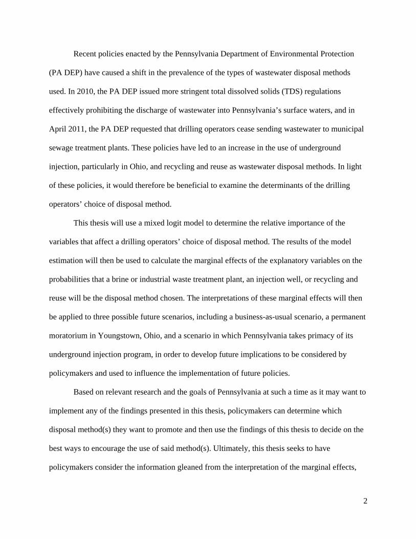
1.1. Background on the Marcellus Shale
The Marcellus Shale is a rock formation that exists primarily beneath Pennsylvania, New
York, West Virginia, and Ohio but underlies very small areas of Maryland, Virginia, Kentucky,
and Tennessee as well, spanning approximately 600 miles, north to south, and covering an area
of approximately 54,000 square miles. It occurs at a depth of between 3,000 and 9,000 feet and is
up to 250 feet thick or more in some areas (Sumi 2008).
Figure 1.1 Extent of and Depth to the Base of the Marcellus Shale
Source: http://geology.com/articles/marcellus-shale.shtml
It is a black shale that is part of the Middle Devonian Series, meaning that it originated
approximately 350-415 million years ago when layers of clay and mud were compressed to form
a sedimentary rock. Dead organic material was also caught in these layers and has since been
5
converted into hydrocarbons, including natural gas (Sumi 2008). It is this reserve of trillions of
cubic feet of natural gas that has caused the Marcellus Shale to attract considerable attention over
the past few years. Many politicians and economists have cited this resource as part of a plan to
end this country’s dependence on foreign oil and create domestic jobs.
The exact estimates of the amount of natural gas contained in the Marcellus Shale
formation have varied over the years due to changing geologic and engineering data and
improvements in the technology used to recover this resource. They also differ in the
terminology used to describe them1. In 2003, the United States Geological Survey (USGS)
released its Assessment of Undiscovered Oil and Gas Resources of the Appalachian Basin
Province, 2002 in which it estimated that the Marcellus Shale contained a mean of
approximately 1.9 trillion cubic feet (tcf) of undiscovered resources. In 2008, Terry Engelder, a
professor of geosciences at the Pennsylvania State University, and Gary Lash, a professor of
geology at the State University of New York at Fredonia, estimated that the Marcellus Shale
contained approximately 500 tcf of gas-in-place, referring to the total volume of natural gas
contained in the formation, not taking into account the technological capability to recover the
resource. Production data from the Barnett Shale in Texas indicated that about 10 percent of its
gas-in-place could be technically recovered. Applying this information to the Marcellus Shale,
Engelder and Lash estimated that the Marcellus Shale would yield 50 tcf of technically
recoverable resources, referring to the volume of gas that is actually able to be produced from
either discovered or yet undiscovered reserves (Engelder and Lash).
1 The Penn State Extension informational sheet “How Much Natural Gas Can the Marcellus Shale Produce?”prepared by David Yoxtheimer of the Penn State Marcellus Center for Outreach and Research, gives a summary of the range of estimates of the amount of natural gas contained in the Marcellus Shale and compiles a list of the accepted definitions used to describe the resource.
6
In 2009, the U.S. Department of Energy’s (US DOE) National Energy Technology
Laboratory (NETL) estimated that the Marcellus Shale contained 1,500 tcf of original gas-in-
place and 262 tcf of technically recoverable resources. The U.S. Energy Information
Administration’s (EIA) Annual Energy Outlook 2011 estimated that the Marcellus Shale
contained 400 tcf of technically recoverable resources. In August 2011, the USGS issued a new
assessment estimating that the Marcellus Shale contained 84 tcf of undiscovered, technically
recoverable resources, referring to gas that can be produced using secondary recovery methods,
regardless of economic viability. Most recently, the EIA’s Annual Energy Outlook 2012
estimated that the Marcellus Shale contained 141 tcf of unproved, technically recoverable
resources, referring to the volume of gas that is predicted to be recoverable in the future, given
available geologic and engineering data, but has not actually been proven to exist based on
accepted geologic information, such as actual drilling production data.
Range Resources – Appalachia, LLC, currently one of the largest natural gas producers in
Pennsylvania, pioneered the development of the Marcellus Shale. In 2003, they drilled an
experimental well in Washington County, Pennsylvania, and met with success through the
utilization of the horizontal drilling and hydraulic fracturing methods that were previously
successful in the Barnett Shale in Texas. Their first Marcellus well began producing in 2005
(“Marcellus Shale – Appalachian Basin”). As of May 2012, a total of 5,338 Marcellus wells have
been drilled by 70 different operators, including 545 so far in 2012 (Kelso).
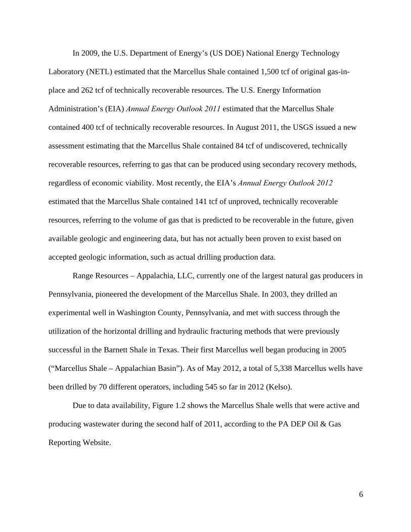
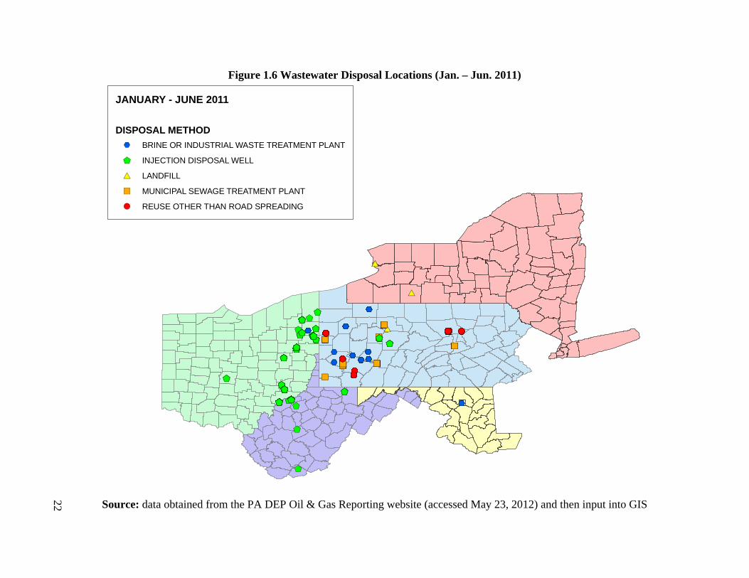
Due to data availability, Figure 1.2 shows the Marcellus Shale wells that were active and
producing wastewater during the second half of 2011, according to the PA DEP Oil & Gas
Reporting Website.
7
Figure 1.2 Active Marcellus Shale Gas Production Well Locations in Pennsylvania (Jul. – Dec. 2011)
Source: data obtained from the PA DEP Oil & Gas Reporting Website (accessed May 23, 2012)
and then input into GIS
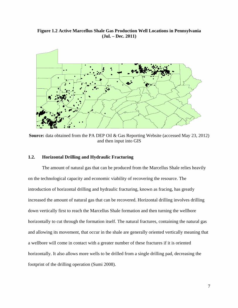
1.2. Horizontal Drilling and Hydraulic Fracturing
The amount of natural gas that can be produced from the Marcellus Shale relies heavily
on the technological capacity and economic viability of recovering the resource. The
introduction of horizontal drilling and hydraulic fracturing, known as fracing, has greatly
increased the amount of natural gas that can be recovered. Horizontal drilling involves drilling
down vertically first to reach the Marcellus Shale formation and then turning the wellbore
horizontally to cut through the formation itself. The natural fractures, containing the natural gas
and allowing its movement, that occur in the shale are generally oriented vertically meaning that
a wellbore will come in contact with a greater number of these fractures if it is oriented
horizontally. It also allows more wells to be drilled from a single drilling pad, decreasing the
footprint of the drilling operation (Sumi 2008).
8
Although the Marcellus Shale does contain natural fractures, they generally are not
porous enough to allow production in commercial quantities and thus fracing is used. This
process, which involves creating artificial fractures, through the injection of millions of gallons
of pressurized water, mixed with sand and chemicals, increases the flow of the natural gas out of
the well (Sumi 2008).
Figure 1.3 Horizontal Drilling and Hydraulic Fracturing
Source: http://geology.com/articles/marcellus-leases-royalties.shtml
1.3. Wastewater Management
The use of millions of gallons of water per well in the fracing process requires that the
drilling operators properly manage the wastewater that is inevitably produced as a result.
Approximately ten percent of the water will return to the surface as flowback water within thirty
days of fracing and must be disposed of or treated properly, as it contains high levels of total
dissolved solids (TDS), fracing chemicals, sand, salt, metals, and even radioactive material from
9
its contact with the shale. Produced water that will return to the surface, along with the natural
gas, when a well is in production must also be properly managed (Abdalla et al. 2011)2.
Discharge into Pennsylvania’s rivers, streams, and lakes is not a disposal option unless
the wastewater is treated first, due to its high levels of TDS that are toxic to the health of aquatic
ecosystems. The Federal Safe Drinking Water Act does not include enforceable TDS standards,
but the Pennsylvania Safe Drinking Water Act does, following new regulations issued by the PA
DEP in 2010. A more stringent standard of 500 mg/L for TDS was introduced. As a result of this
new standard, it has become necessary to utilize alternative treatment and/or disposal methods,
including dilution at a municipal or industrial brine treatment plant, direct reuse without
treatment by blending the flowback water with freshwater, on- or off-site treatment and reuse, or
off-site disposal in an underground injection well (Abdalla et al. 2011).
In 2007 and early 2008, dilution at municipal treatment facilities and then discharge into
surface waters was a fairly common disposal method because of its convenience and low cost
($0.05-$0.065/gal). However, municipal sewage treatment plants are not properly equipped3 to
remove the high levels of TDS found in Marcellus Shale wastewater (dilution is the only option
at these facilities), which means that the discharged water is still quite briny (Abdalla et al.
2011). The PA DEP realized that Pennsylvania’s surface waters would not be able to continue to
absorb these still relatively high levels of TDS so in 2008 the PA DEP imposed a limit on
municipal sewage treatment plants, allowing them to only accept 1% of their daily intake as
natural gas drilling wastewater, and then in 2010 the PA DEP issued the new TDS regulations
(as described above) (“Our Look”). Under these new regulations, 27 facilities that had
2 According to Table 1.2, approximately 25.2 million gallons of wastewater, both flowback and produced water, was generated in 2011. 3 The municipal sewage treatment plants are also not properly equipped to deal with the radioactive materials that are present in the wastewater due to the water’s contact with the shale.
10
historically accepted natural gas drilling wastewater were allowed to continue doing so as long as
their daily intake did not increase. Between 2010 and 2011, twelve of those grandfathered
facilities voluntarily ceased accepting drilling wastewater. Then on April 19, 2011, the PA DEP
issued a press release calling on all Marcellus Shale natural gas drilling operators to stop sending
drilling wastewater to the remaining fifteen municipal sewage treatment plants that were still
accepting it by May 19, 2011 (Commonwealth of Pennsylvania). Thus, as a result of the more
stringent TDS regulations and the PA DEP request, drilling operators have turned to other
disposal and/or treatment options. In particular, disposal in underground injection wells and the
recycling and reuse of wastewater have become increasingly attractive alternatives to drilling
operators.
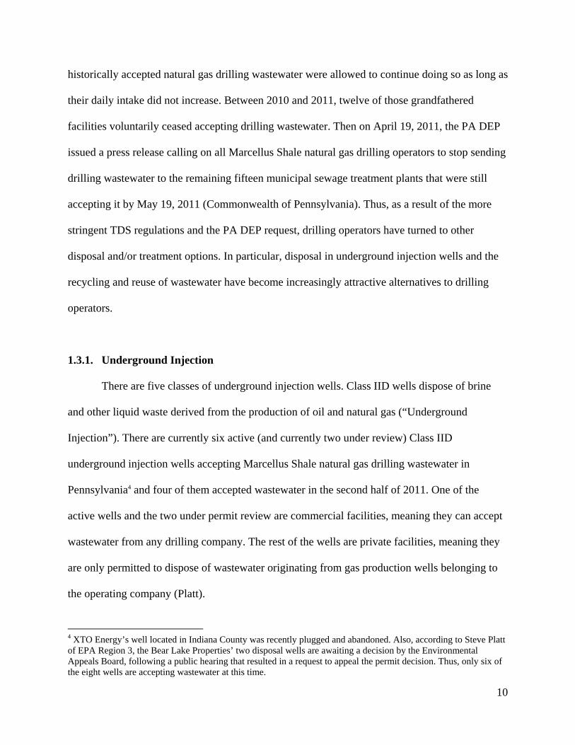
1.3.1. Underground Injection
There are five classes of underground injection wells. Class IID wells dispose of brine
and other liquid waste derived from the production of oil and natural gas (“Underground
Injection”). There are currently six active (and currently two under review) Class IID
underground injection wells accepting Marcellus Shale natural gas drilling wastewater in
Pennsylvania4 and four of them accepted wastewater in the second half of 2011. One of the
active wells and the two under permit review are commercial facilities, meaning they can accept
wastewater from any drilling company. The rest of the wells are private facilities, meaning they
are only permitted to dispose of wastewater originating from gas production wells belonging to
the operating company (Platt).
4 XTO Energy’s well located in Indiana County was recently plugged and abandoned. Also, according to Steve Platt of EPA Region 3, the Bear Lake Properties’ two disposal wells are awaiting a decision by the Environmental Appeals Board, following a public hearing that resulted in a request to appeal the permit decision. Thus, only six of the eight wells are accepting wastewater at this time.
11
The permit for the Range Resources well, located in Erie County, was originally issued to
NEA Cross Company in November 1985 and has since been transferred to several different
operators. It is now operated by Range Resources. Its ten-year permit expired in January 2011
and a new one was issued following a public hearing in June 2011 (U.S. EPA, Region 3, Range
Resources). The permit for the CNX Gas Company well, located in Somerset County, was
originally issued to Dominion Exploration Production in May 2001. Then in April 2012
CONSOL Energy Holdings, LLC purchased Dominion and after corporate restructuring CNX
Gas Company LLC took control in January 2011. Its 10-year permit expired in May 2011 and a
new one was issued following a public hearing in June 2011 (U.S. EPA, Region 3, Jenner
Township, PA). The permit for one of the two EXCO Resources wells, located in Clearfield
County, was issued to EOG Resources in May 2005. It is a ten-year permit and therefore will
remain in effect until May 2015. The permit was transferred to EXCO Resources in June 2008
(U.S. EPA, Region 3, Consent Agreement).
Figure 1.4 shows the location of the wells and Table 1.1 indicates their injection volume
(bbls/month) and maximum surface injection pressure (psi). The injection volume refers to the
maximum allowable volume of wastewater that can be injected into each well on a monthly
basis. The surface injection pressure is the maximum allowable pressure at which wastewater can
be injected (the pressure just below that which would fracture the rock). Once a well approaches
its maximum surface injection pressure (or instantaneous shut-in pressure) it means the well is
approaching its maximum capacity. Several wells have been in operation since the 1980s and
have not yet approached their maximum capacity, indicating that the injection formations have
good injectivity, transmissivity, and high capacity potential. This is contrary to the popular belief
that Pennsylvania’s geology is unsuitable for underground injection. Rather, the limited number
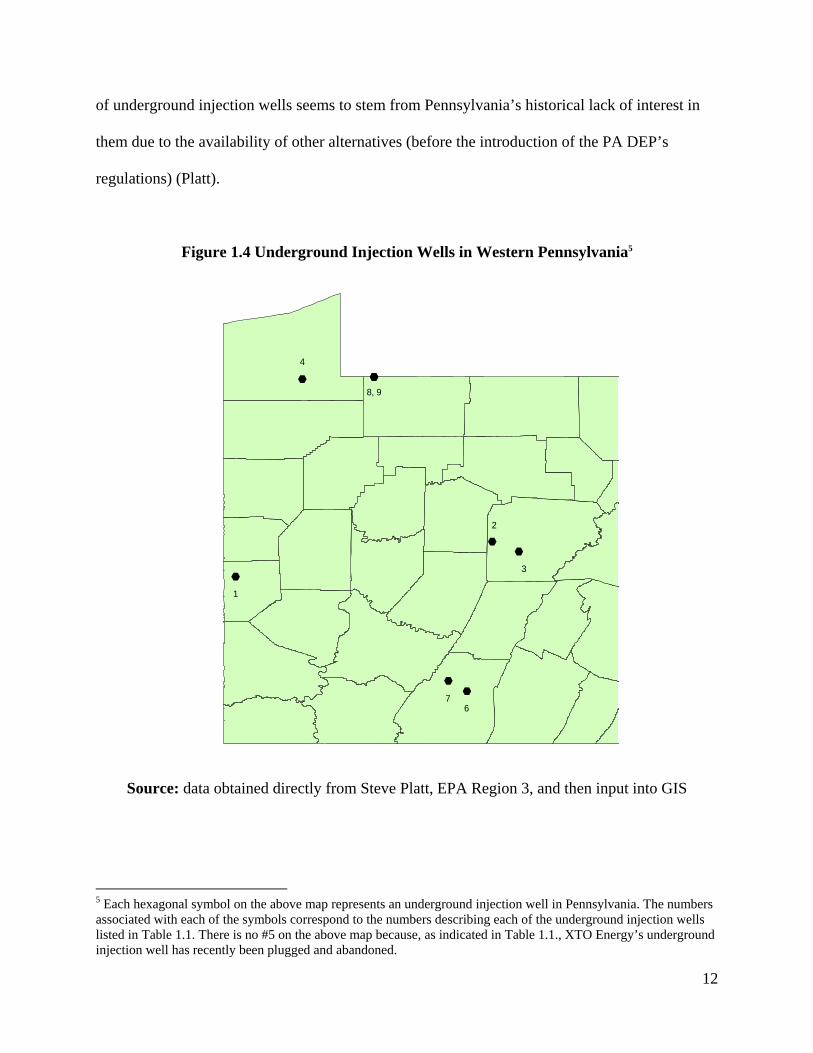
12
of underground injection wells seems to stem from Pennsylvania’s historical lack of interest in
them due to the availability of other alternatives (before the introduction of the PA DEP’s
regulations) (Platt).
Figure 1.4 Underground Injection Wells in Western Pennsylvania5
Source: data obtained directly from Steve Platt, EPA Region 3, and then input into GIS
5 Each hexagonal symbol on the above map represents an underground injection well in Pennsylvania. The numbers associated with each of the symbols correspond to the numbers describing each of the underground injection wells listed in Table 1.1. There is no #5 on the above map because, as indicated in Table 1.1., XTO Energy’s underground injection well has recently been plugged and abandoned.
%,
%,
%,
%,
%,
%,
%,%,
1
2
3
4
67
8, 9
13
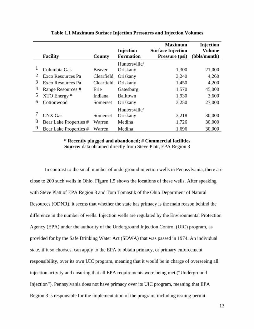
Table 1.1 Maximum Surface Injection Pressures and Injection Volumes
Facility County Injection Formation
Maximum Surface Injection
Pressure (psi)
Injection Volume
(bbls/month) 1 Columbia Gas Beaver
Huntersville/ Oriskany 1,300 21,000
2 Exco Resources Pa Clearfield Oriskany 3,240 4,2603 Exco Resources Pa Clearfield Oriskany 1,450 4,2004 Range Resources # Erie Gatesburg 1,570 45,0005 XTO Energy * Indiana Balltown 1,930 3,6006 Cottonwood Somerset Oriskany 3,250 27,000 7 CNX Gas Somerset
Huntersville/ Oriskany 3,218 30,000
8 Bear Lake Properties # Warren Medina 1,726 30,0009 Bear Lake Properties # Warren Medina 1,696 30,000
* Recently plugged and abandoned; # Commercial facilities Source: data obtained directly from Steve Platt, EPA Region 3
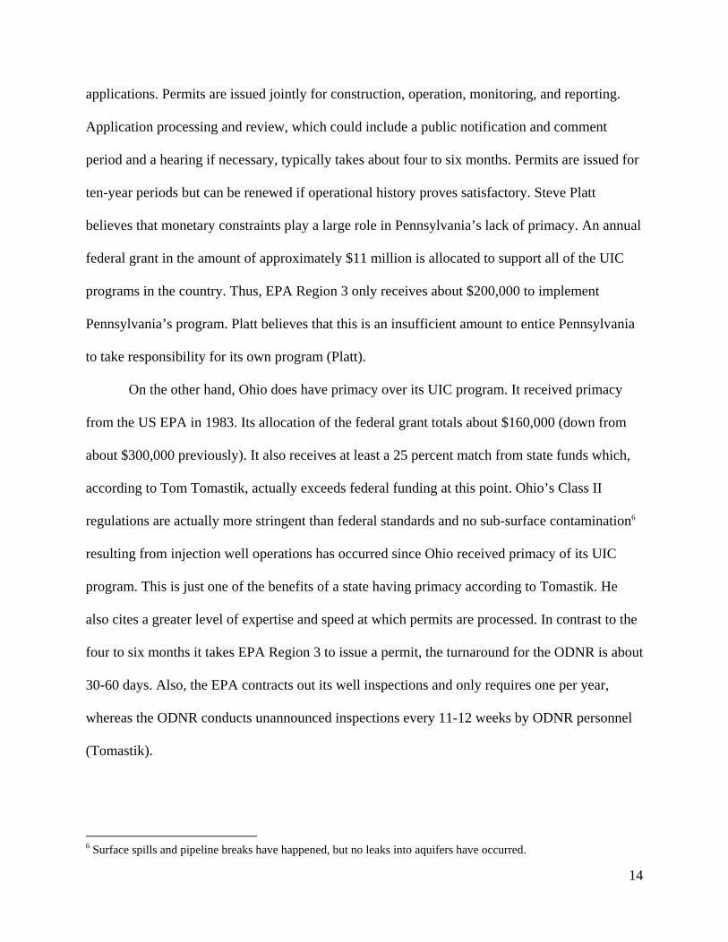
In contrast to the small number of underground injection wells in Pennsylvania, there are
close to 200 such wells in Ohio. Figure 1.5 shows the locations of these wells. After speaking
with Steve Platt of EPA Region 3 and Tom Tomastik of the Ohio Department of Natural
Resources (ODNR), it seems that whether the state has primacy is the main reason behind the
difference in the number of wells. Injection wells are regulated by the Environmental Protection
Agency (EPA) under the authority of the Underground Injection Control (UIC) program, as
provided for by the Safe Drinking Water Act (SDWA) that was passed in 1974. An individual
state, if it so chooses, can apply to the EPA to obtain primacy, or primary enforcement
responsibility, over its own UIC program, meaning that it would be in charge of overseeing all
injection activity and ensuring that all EPA requirements were being met (“Underground
Injection”). Pennsylvania does not have primacy over its UIC program, meaning that EPA
Region 3 is responsible for the implementation of the program, including issuing permit
14
applications. Permits are issued jointly for construction, operation, monitoring, and reporting.
Application processing and review, which could include a public notification and comment
period and a hearing if necessary, typically takes about four to six months. Permits are issued for
ten-year periods but can be renewed if operational history proves satisfactory. Steve Platt
believes that monetary constraints play a large role in Pennsylvania’s lack of primacy. An annual
federal grant in the amount of approximately $11 million is allocated to support all of the UIC
programs in the country. Thus, EPA Region 3 only receives about $200,000 to implement
Pennsylvania’s program. Platt believes that this is an insufficient amount to entice Pennsylvania
to take responsibility for its own program (Platt).
On the other hand, Ohio does have primacy over its UIC program. It received primacy
from the US EPA in 1983. Its allocation of the federal grant totals about $160,000 (down from
about $300,000 previously). It also receives at least a 25 percent match from state funds which,
according to Tom Tomastik, actually exceeds federal funding at this point. Ohio’s Class II
regulations are actually more stringent than federal standards and no sub-surface contamination6
resulting from injection well operations has occurred since Ohio received primacy of its UIC
program. This is just one of the benefits of a state having primacy according to Tomastik. He
also cites a greater level of expertise and speed at which permits are processed. In contrast to the
four to six months it takes EPA Region 3 to issue a permit, the turnaround for the ODNR is about
30-60 days. Also, the EPA contracts out its well inspections and only requires one per year,
whereas the ODNR conducts unannounced inspections every 11-12 weeks by ODNR personnel
(Tomastik).
6 Surface spills and pipeline breaks have happened, but no leaks into aquifers have occurred.
15
Figure 1.5 Underground Injection Wells in Ohio
Source: data obtained directly from Tom Tomastik, ODNR, and then input into GIS
1.3.1.1. Seismic Activity
Underground injection has been in the news recently due to a collection of twelve
earthquakes that occurred in eastern Ohio throughout 2011 that have possibly been linked to this
disposal method. On December 31, 2011 a magnitude 4.0 earthquake occurred near an injection
well in Youngstown, Ohio (Mahoning County). It was the twelfth earthquake to occur in the area
since March 2011 and the strongest yet, as the others were about 2.1 to 2.7 in magnitude.
Following an earthquake on December 24, 2011, the director of the ODNR requested, on
December 30, that D&L Energy Inc. halt injection at the Northstar 1 well; the company did so
16
voluntarily. Then, following the latest, strongest earthquake on December 31, state officials
instituted a moratorium on all injection activity within a five-mile radius of the Northstar 1 well.
This moratorium applies to three wells in the area that were under construction at the time. It also
resulted in the permit for another well in the area being put on hold (Ohio Department of Natural
Resources).
In March 2012, the ODNR issued a preliminary report on the seismic activity that
occurred in the vicinity of Youngstown, Ohio. Prior to the March 2011 earthquake, there had
been no record of any earthquakes with epicenters located in Mahoning County, but now a series
of seemingly coincidental events appears to point to evidence of injection activity at the
Youngstown well inducing the recent seismic activity. The Northstar 1 well commenced
injection activity in December 2010, three months before the first earthquake, and the subsequent
earthquakes were all located in proximity to the wellbore. The focal depths of these seismic
events were determined to be approximately 4,000 ft laterally and 2,500 ft vertically from the
wellbore terminus once monitoring equipment was put in place. There also appears to be
evidence of fractures within the Precambrian rock formation, the well’s injection layer (Ohio
Department of Natural Resources).
Due to the evidence of possible induced seismicity from injection well activity, the report
goes on to make recommendations to better monitor underground injection wells and protect the
health and safety of Ohio’s citizens. These changes, if adopted, would make Ohio’s regulations
the most stringent in the nation. The recommendations include not locating new injection wells
within known faulted areas; submitting, at the time of permit application, any information
regarding the existence of known faults within a certain radius of the proposed well; conducting
seismic surveys; conducting an injection test, prior to initial injection, to determine the formation
17
parting pressure and injection rates; requiring the installation of a continuous pressure
monitoring system and an automatic shut-off system that would be activated if the maximum
injection pressure were to be exceeded; and requiring the installation of an electronic data
recording system to track all injection fluids from “cradle to grave”7 (Ohio Department of
Natural Resources).
Following these recommendations by the ODNR, Ohio Governor John Kasich issued an
executive order on July 10, 2012, immediately enacting new state regulations on underground
injection wells used to dispose of natural gas drilling wastewater. The order gives the ODNR the
authority to implement their recommendations and gives the chief of the Division of Oil and Gas
Resources Management authority to order preliminary tests at proposed well sites, prevent
drilling at any sites that fail these preliminary tests, limit injection pressure, monitor for any
leakages, and order the installation of automatic shut-off systems. This order does not affect the
regional moratorium that was instituted following the recent earthquakes in the Youngstown
area8. The order will remain in effect for ninety days, allowing the state’s legislators to formally
pass a law making the regulations permanent (“Kasich”).
The case of Youngstown, Ohio, is not the first instance of the possibility of injection
activity inducing seismic activity. In 2011, state officials in Arkansas shut down some injection
wells and then instituted a permanent moratorium after a “swarm”9 of earthquakes occurred in
the north-central part of the state and was linked to the underground injection of wastewater
7 This new requirement would also help in the comparison and verification of wastewater data from Pennsylvania and Ohio. This issue is discussed further in Section 6.1.1. 8 In February 2012, D&L Energy, the Youngstown well’s operator, sought permission from the state of Ohio to resume disposal operations at the injection well. As of April, though, it had not yet received such permission due to the ongoing nature of the moratorium (“Kasich”). 9 An earthquake swarm is defined as an event in which a local area experiences a sequence of earthquakes striking in a relatively short period of time; no earthquake in the sequence can be identified as the main event (Soraghan).
18
originating from the Fayetteville Shale. Since then a scientist at the Center for Earthquake
Research and Information at the University of Memphis published a paper citing underground
injection as the cause. Also, according to scientists at the University of Texas, Austin, several
small earthquakes that occurred near the Dallas-Fort Worth International Airport in 2008 and
2009 were linked to an underground injection well drilled in September 2008. This resulted in
two wells being shut down (Soraghan). In May 2012, two more earthquakes occurred in eastern
Texas, near the Louisiana border, in an area home to several injection wells. Scientists are still
determining whether these recent seismic events can be linked to underground injection as well
(Kenworthy).
1.3.2. Recycling
The recycling and reuse of natural gas drilling wastewater is the management method that
has experienced the largest increase in use over the past six months (beginning of 2011 to end of
2011) (a 150 percent increase, according to Table 1.2) and now represents 87 percent of the
wastewater disposal/treatment total. In March 2012, the PA DEP announced the revised Residual
Waste Beneficial Use general permit (the new WMGR123) that encourages the recycling of
wastewater that results from oil and gas drilling. Previously there existed three different general
permits, WMGR119, WMGR121 and WMGR123, but the new permit consolidates them into
one that will improve institutional efficiency while better protecting Pennsylvania’s waterways
through the minimization of surface water withdrawal and discharge. It promotes the use of a
closed-loop process, meaning that after wastewater has been treated and processed at dedicated
recycling facilities it is then sent back out into the field and reused at other drill sites (e.g. to frac
other natural gas wells) because these facilities’ permits allow no liquid discharge into streams.
19
The permit also establishes water quality criteria, based on drinking water and in-stream water
quality standards, which, if met, allow the treated and processed water to be stored and
transported as freshwater. Water that does not meet these standards will continue to be stored in
tanks or impoundment pits and transported as residual waste. There are currently ten facilities
operating under one of the previous general permits and they will continue to operate under the
new revised permit. There are also ten new facilities that have submitted permit applications to
the PA DEP (Pennsylvania Department of Environmental Protection).
1.3.3. On-Site Treatment and Reuse
The reuse of wastewater is often done in the field and involves either a mobile treatment
unit or dilution with freshwater. The mobile units can be dispatched directly to the drilling site
(or might be stationed at strategic locations around the state) and are able to treat flowback water
for frac additives and TDS, provide disinfection against bacteria, and generate a solids sludge
that is safe for disposal at a landfill. The process could involve pretreatment (reduction of TDS
and disinfection), evaporation to produce reusable freshwater, and crystallization to produce
reusable salt products. On-site treatment and reuse reduces the volume of wastewater removed
from and freshwater brought to the drilling site, reducing truck traffic (as well as the distances
the trucks travel). If on-site treatment is not utilized, drilling companies will often just dilute the
flowback water with additional freshwater before reusing it (Mittal).
20
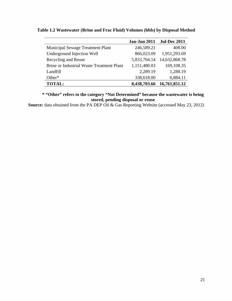
1.4. Wastewater Numbers
According to the data sourced from the PA DEP Oil & Gas Reporting Website,
summarized in Table 1.2, in the first half of 2011, 246,589 barrels (bbls, 1 bbl = 42 gallons) of
wastewater were disposed of at nine municipal sewage treatment plants. That amount decreased
to 408 bbls at two facilities in the second half of 2011, after the PA DEP requested that drilling
operators cease sending drilling wastewater to municipal sewage treatment plants. This is an
example of how policy can influence wastewater disposal.
Conversely, in the first half of 2011, only 866,023 bbls of wastewater were disposed of in
32 underground injection wells, but, by the second half of 2011, 1,951,293 bbls were injected in
51 wells, an increase of 125 percent. In the second half of 2011, four Pennsylvania underground
injection wells accounted for 11,795 bbls of wastewater disposal or 0.6 percent of the share of
wastewater that was disposed of in underground injection wells; five West Virginia injection
wells accounted for 15,121 bbls or 0.8 percent of the injection total; and 42 Ohio injection wells
accounted for 1,924,377 bbls or 98.6 percent of the injection total. Recycling and reuse also
increased during this time period, from 5,833,704 bbls, in the first half of 2011, to 14,632,869
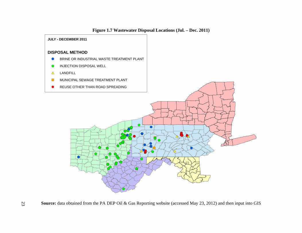
bbls in the second half of 2011, representing a 150 percent increase. Figures 1.6 and 1.7
demonstrate the change in the type and number of each disposal method being utilized between
and first and second six-month periods of 2011.
21
Table 1.2 Wastewater (Brine and Frac Fluid) Volumes (bbls) by Disposal Method
Jan-Jun 2011 Jul-Dec 2011 Municipal Sewage Treatment Plant 246,589.21 408.00 Underground Injection Well 866,023.09 1,951,293.69 Recycling and Reuse 5,833,704.14 14,632,868.78 Brine or Industrial Waste Treatment Plant 1,151,480.03 169,108.35 Landfill 2,289.19 1,288.19 Other* 338,618.00 6,884.11 TOTAL: 8,438,703.66 16,761,851.12
* “Other” refers to the category “Not Determined” because the wastewater is being
stored, pending disposal or reuse Source: data obtained from the PA DEP Oil & Gas Reporting Website (accessed May 23, 2012)
22
Figure 1.6 Wastewater Disposal Locations (Jan. – Jun. 2011)
Source: data obtained from the PA DEP Oil & Gas Reporting website (accessed May 23, 2012) and then input into GIS
!(!(
$+
!(
$+
!(
$+%,
$+ %,
%,%,
%,%,%,
%,%,
%,
%,
%,%,
$+$+ $+
%,
%,
%,
%,
%,%,%,
%,
%,%,
%,
%,
%,
$+%,
%,%,%,
$+
%,%,
%,
%,
%,%,%,%,%,
%,
%,
%,%,
$+$+ $+$+%,
$+
%,
%,%,
%,")
%,
$+%,
%,%,%,
!(%,
%,
%,!(
$+
%,%,%,
$+
%,%,
$+
%,
%,
%,%,
%,%,
%,
$+%,%,%,
%,
%,
%,
$+ %,
%,
$+
%,
%,
")
$+
")
%,
$+
%,
%,%,
$+
$+
")
%,
$+%,
!(%,
")
!(%,
")
!(!(!(!(!(!(!(!(!(%,
!(%,
!(%,
!(%,
!(%,%,%,
!(%,
!(%,
!(!(!(%,
!(%,
!(%,
!(%,
!(
$+$+$+
!(!(!(!(!(!(!(
%,
")
!(
")
%,!(
%,
%,!(
%,
%,!(
%,
!(!(!(%,
!(
%,
%,!(
%,
%,!(
%,
%,!(
%,!(
%,%,!(
%,!(
%,!(
%,!(
%,!(
%,!(
%,!(
%,!(
%,!(
%,!(
%,!(
%,!(!(
%,
!(
%,
!(
%,
%,!(
%,!(
%,!(
%,!(
%,!(
%,!(
%,!(
$+
%,!(
%,!(
%,!(
%,!(
%,!(
%,!(!(!(!(!(!(!(!(!(
%,!(
%,
%,!(
%,
%,!(
%,
%,!(
%,
%,!(
%,
%,!(
%,
%,!(
%,
%,!(
%,
%,!(
%,!(
%,!(
%,!(
%,!(
%,!(
%,!(
%,!(
%,!(
%,
%,!(
%,
%,!(
%,
%,!(
%,
%,!(
%,!(
%,!(
%,!(
%,!(
%,!(
%,!(
%,%,%,
%,
%,
%,
%,
%,
%,
%,
%,
%,
%,
%,
%,
%,
!(!(!(%,%,%,%,%,%,%,
!(!(!(!(!(!(!(!(!(%,
!(
%,
%,!(
%,
%,!(
%,
%,!(
%,
%,!(
%,
%,!(
%,
%,!(
%,
%,!(
%,
!(
")
%,!(
%,!(
%,!(
%,!(
%,!(
%,!(
%,!(
%,!(
%,!(
%,!(
%,!(
%,!(
%,!(!(
$+$+
!(!(!(!(!(!(!(
")$+
!(!(
%,%,%,%,%,
!(!(!(!(!(!(!(!(!(!(!(!(!(!(!(!(!(!(!(!(!(
$+
!(!(!(!(!(!(!(!(!(!(!(!(!(
")
!(!(
")")")$+ ")")
!(!(!(!(!(!($+
%,
!(!(!(!(
%,%,%,
%,
%,%,
$+ !($+$+ !(
!(
!(
!( %,
$+
%,
!(
$+!(
%,
%,
%,
%,
!(!($+
%,
%,$+
%,
!($+
%,
%,$+
%,
$+%,$+
%,$+$+ $+$+$+ !($+
%,
$+
%,
!($+
%,
%,$+
%,%,%,
!($+
%,
%,$+
%,
!($+ $+
%,
%,$+
%,
$+
%,
!(
$+
!(
$+
!($+
%,
$+%,
%,
%,
%,
!($+
%,
$+%,
%,
%,
%,
!($+
%,
$+%,
%,
%,
%,
$+%,
%,%,
!($+
%,
$+%,
%,
%,
%,
%,!(!(!(!(!($+ $+
%,$+ $+%, !($+ $+%,
%,%,
%,%,
%,%,%,%,%,
!($+
%,
$+$+
%,
$+
%,
%,
")
%,
$+
%,
%,
")$+
%,
%,
")
%,
$+
%,%,
!($+
!($+$+
%,
$+
%,
%,
$+")")!(
%,%,%,
%,
$+ !(%,
%,
!(
$+$+
%,
%,%,%,
%,
%,
%,%,
$+$+
%,
%,%,
!(
%,!(
%,
%,
$+")$+%,
%,
")
$+%,
%,
")
$+
$+%,
%,
")
$+
$+%,
%,
")")
$+%,
%,
")
$+
$+%,
%,
")
$+
")%,
#*
!( %,
$+
$+%, ")
$+
$+
$+%,
%,
$+
")
$+
$+%,
%,
")
$+
")
$+
$+%, ")
")
$+
$+%,
%,
")
$+
$+
$+%,
%,
")")
$+
$+%,
%,
")
$+
")
$+
$+%,
%,
")
$+
")
$+
$+%,
%,
")
$+
")%,
$+
$+%,
%,
")
$+
$+%, ")
$+
")
%,
%,%,%,%,%,
$+
$+%,
%,
")")
$+
$+%,
%,
")
$+
")
$+
$+%,
%,
$+
")%,
$+
$+%,
%,
")
$+
")
$+
$+%,
%,
")")
$+
$+
$+
$+!(
%,
%, ")%, ")%, ")
$+
%,
%,
")
$+
%, ")
$+
%,%,%,%,%,%,%,%,
%,%,
!(
$+
%,
%,
$+
%,
$+
!(
!(
$+
!(
$+$+
%,
!(
!(
$+
!(
!(
$+
%,
!(
$+
%,
$+
!(!(
$+
%,%,
!(
$+
$+
%,
!(
!(
$+
%,
%,
!(
!(
$+
%,%,
!(
$+
$+ !(
$+
%,
!(
$+
%,
!(
!(
$+
$+
%,%,
$+
$+
$+
!(
$+
%,
!(
!(
$+
%,
$+
!(
$+
$+
%,
$+
!(
$+
%,
%,
!(!(
$+
%,
!(
$+
!(
$+
%,
%,
!(
!(
$+
%,
%,%,
$+
!(
$+
%,
%,%,
!(
$+
%,
%,
!(
!(
$+
%,%,
$+
!(
$+
%,%,
$+
%,
$+
!(
$+
!(
$+
%,
!(
!(
$+
%,
!(
!(
$+
%,
%,
!(
$+
$+
%,
!(
$+
$+
%,
$+
!(
$+
$+
%,
$+
!(
!(
$+
%,
!(
$+
$+
%,
$+
!(
!(
$+
%,%,
$+
$+
$+$+
$+%,
%,
$+
!(
!(
$+
$+
%,
%,%,
!(
$+
%,
!(
$+
%,
!(
!(
$+
$+
%,
%,
$+
!(
$+
%,
%,
!(
$+
%,
!(
$+
%,
!(!(
$+
%,%,
!(
$+
$+
%,
%,%,
!(
$+
$+
$+
!(
$+
$+
$+$+$+
!(")
$+
%,
$+
!(
$+
$+
%,%,
!(
$+
%,
$+$+
!(
$+
!(
$+
%,
!(
!(
!(
$+
$+
$+
$+
$+
!(!(
!(!(
$+
%,
$+
%,%,%,%,
$+
!(!(
!(
$+
%,
$+%,
%,%,
$+
!(
!(
$+
%,%,
$+
%,%, %,%,%,
$+
!(
!(!(
%,
$+
%,
$+%,
%,%,%,
$+
!(!(
!(
$+
$+
%,%,
$+%,
%,%,%,
$+
!(
!(
$+
%,%,
$+%,
%,%,%,%,
$+
!(
!(%,
!(
!(
$+!(
!(
$+!(
!(
!(
!(
!(
!(
!(
!(
!(
!(
!(
!(
!(
!(
!(!(
")
$+
$+
%,%,
$+
!(
$+!(
!(!(
$+
!(!(
$+
!(
$+
!(!(
$+
%,
%,%,%,%,
$+
!(
!(
$+!(
$+
%,
%,%,
$+
%,
%,%,
%,
$+$+
!(
")
$+
%,
!(
!(
$+
$+
%,
$+
$+
%,
$+
!($+
$+$+
!(
$+
$+
%,
$+
%,
$+
!(
$+
$+
$+
!(
$+
$+
%,
$+
!(")
$+
$+
%,
!(
!(
$+
$+
%,
$+$+$+
$+
%,
$+
!(
!(
$+
%,
!(
$+
%,
$+
!(")
$+$+
!(
!(
$+
$+
$+
%,
!(
!(
$+
%,
$+$+%,
!(
$+
$+
%,
$+$+$+
$+ !(
$+
%,
$+
%,
!(
$+
$+
%,
$+
!(
$+
$+
%,
$+
!(
$+
$+
%,
$+
!(
$+
$+
%,
$+
%,
!(
!(
$+
$+
%,%,
$+$+
$+
%,
!(
$+
$+
%,
$+
")
$+
$+
$+
%,
!(")
$+
$+
%,
$+
!(
!(
$+
$+
%,
$+
")
$+
!(
$+
!(
!(
$+
%,
%,%,
!(
!(
")
$+
$+
%,
$+
")
!(
!(
$+
%,
$+
!(
!(
$+
%,
$+
!(
$+
$+
%,
$+
$+
!(
!(
$+
%,
$+$+
")
!(
!(
")
$+
%,
%,
$+
")
%,
!(
$+
%,
$+
!(
#*
%,
!(
$+
%,
!(
$+
%,
$+
")")")")
%,
$+
!(!(
$+$+
%,
")")
!(
!(
$+
$+
%,
$+
!(
!(
$+
%,%,
$+
")")")")
!(
$+
%,
!(
!(
$+
$+
%,
$+
!(
$+
$+
$+
!(
!(
$+
$+
%,
%,%,
$+
!(
$+
$+
%,
$+
")")")")")
$+$+$+$+
%,
!(
$+
%,
%,
$+$+$+
$+%,
$+$+ $+
%,
!(!(
$+$+ $+$+
%,
%,
!(
$+
%,
$+
!(
$+
$+
%,
$+
!(
$+
$+
$+%,
%,
$+
$+
%,
!(
$+$+ $+
%,
!(
!(
$+
")")")")
!(
!(
$+
$+
%,%,
$+
$+
")
$+
$+
%,
$+
")
$+
$+
$+
!(
$+$+ $+
%,
$+
$+$+ $+
%,
")")
$+
$+
%,
$+
!(
$+
$+
$+
%,%,
$+
$+
$+
$+
$+
")")
!(
$+$+ $+
%,
!(
$+$+ $+
%,
!(
!(
$+
$+%,
%,
$+
!(!(
!(
$+$+$+
$+
$+
%,
!(!(
$+
$+$+ $+$+%,
")")")
!(
$+
$+
%,
!(
$+$+ $+$+%,
")")")")")")
!(!(
$+$+ $+$+%,
$+
!(
!(
$+
$+
$+
%,%,
!(
!(
$+
$+
%,
$+
!(
!(
$+
$+
%,
$+
!(
!(
$+
$+
$+
%,
$+
!(
$+$+
!(
$+
$+%,
%,%,
$+
!(
$+
$+
%,
$+
!(
$+$+ $+
%,
!(
$+$+ $+$+%,
!(
!(
$+$+
$+
$+
%,%,
!(
!(
$+$+ $+
%,
!(
$+
$+%,
%,")
!(
$+$+ $+
%,
!(
$+$+
$+
$+
%,
!(
$+$+ $+
%,
!(
!(
$+
$+
%,
%,
$+$+
%,%,
")")")")
!(
$+$+
!(%,
!(
$+$+$+ $+
%,%,
$+
$+%,
$+$+ $+
%,
!(
$+$+ $+
%,
!(
!(!(
%,%,
!(
!(
%,%,
!(!(
!(
%,%,%,
!(
$+$+
%,
$+
%,
$+$+
%,
$+$+ $+
%,
$+$+ $+
%,
!(
%,
%,
!(
%,
$+$+ $+
%,
$+
!(
$+
!(
!(
!(
!(
")
!(
%,
!(!(")
!(
$+
%,
!(!(!(!(!(!(
!(
$+
!(
$+
!(
%,
%,%,
$+
%,%,")
%,%,%,
$+$+
%,
!($+
%,%,%,
$+$+
%,%,%,
$+
%,%,%,
$+
%,%,
$+
%,%,%,
%,
$+$+
%,
%,
%,
%,$+$+
%,%,%,
%,%,
$+%,
%,%,%,
!(!(!(!(!(!(!(%,
")")
!(%,
")")
!(%,
")")
!(!(%,
")
!(
")
!(!(
")
!(!(!($+
%,
$+ ")
!(%,
")
!(!(!(!(!(
%,
!(!(%,
%,
$+$+
!(
#*
!(
%,
$+$+
!(!(!($+
%,
%,
$+ ")")
!(!(%,
$+ ")
!(
")
!(
")
!(!(!(!(%,
!(!(!(!(%,
")
!(!(!(%,
")
!(!(
")
!(!(%,
")
!(!($+
%,
$+ ")")
!(!(!(!($+
%,%,
%,
$+ ")")
!(%,
")
!(!(%,%,
%,%,
%,
$+$+
!(!(!(%,
%,
$+$+
!(!(%,
%,%,
$+
%,%,%,
$+
%,!(!(
%,
%,
$+$+
!(!(%,
")
!(!($+
%,%,
$+
!(
%,
!(!(!(%,%,
$+ ")
!(!(%,
!( !(!(!(!(!(!( !(!(!(%,%,
%,%,
%,
$+$+
!(!(
$+$+
!(!(
$+
!(!(!(#* !(!(!(
$+
!(!(%,%,
$+
%,%, ")
$+
%, ")
$+
$+
$+
%,
$+
%,
$+
%,
")
%,
%,%,
%,%,%,
%,
%,
%,
%,
%,
%,
%,
%,%,
%,
%,%,
%,
%,%,
%,
%,
")
%,%,!( %,
#*
!( %,%,%,
")")
%,!(!(!(
")
")
")
")
")
!(
")")")")
")
")
")
")
")
")
")
")
")
")
")
")
")
")")
%,
")
")
")
")
%,
")
")$+$+
")
")
%,%,!(!(
%,!(
%,!(
%,!(!(!(!(!(!(
%,!(
%,!(
%,!(
%,!(!(
%,%,%,!(!(
%,
!(%,
!(%,
!(%,
!(%,
!(%,
!(%,
!(%,
!(%,
!(%,
!(%,
!(!(!(!(!(!(!(%,
!(
%,
%,!(
%,
%,!(
%,
%,!(
%,
%,!(
%,
%,!(
%,
%,!(
%,!(
%,!(
%,%,!(!(!(!(!(!(!(!(!(!(!(
%,!(
%,!(
%,!(
%,!(
%,!(!(!(!(!(!(!(!(!(!(!(!(!(!(!(!(!(!(!(!(!(!(
$+$+$+$+$+$+$+$+$+$+$+$+$+$+$+$+$+$+$+$+$+$+
$+$+$+$+$+$+$+$+
$+$+$+
$+$+$+
$+$+$+$+$+
$+$+$+$+
$+$+
$+$+
$+$+
$+$+$+$+$+
$+$+$+
$+$+$+$+$+$+$+$+$+
$+$+$+
%,
$+$+$+
$+$+
$+$+$+
$+
%,
$+$+%,
$+$+$+$+$+%,$+
$+$+%,$+
$+$+
$+$+$+$+$+$+
$+
$+%,
$+$+$+$+%,
$+$+
$+
$+$+$+$+$+$+$+$+
$+ $+
$+$+$+
$+$+%,
$+$+%,
$+$+
$+$+$+
%,$+$+$+
%,$+$+$+
%,
$+$+$+
$+$+%,$+
$+$+%,
$+$+$+$+%,$+
$+$+%,
$+$+
$+$+
$+$+$+$+$+
$+$+%,$+
$+$+%,$+
$+$+%,$+
$+$+%,
$+$+$+
")%,
$+$+$+
$+$+$+$+
$+$+$+
$+$+$+
$+$+$+
$+$+$+
$+$+$+$+
$+$+$+
$+$+
$+$+$+
$+$+$+$+
$+$+$+$+$+$+
$+$+%,$+
$+$+%,$+
$+$+%,$+
$+$+$+$+
$+$+%,$+
$+$+%,$+
$+$+%,$+
$+$+%,$+
$+$+%,$+
$+$+%,$+
$+$+$+$+
$+$+%,
!(
!(
$+
$+
$+
%,$+$+$+
%,$+$+$+
%,$+$+$+
%,$+$+$+
%,$+$+$+
%,$+$+$+
%,$+$+$+$+
$+$+$+$+
%,$+$+$+$+
%,$+$+$+$+
%,
!(
$+
$+ !(
$+
$+
$+
%,
$+
$+$+$+
%,$+$+$+
%,$+$+$+
%,$+$+$+
%,$+$+$+
%,$+$+$+
%,
$+$+$+$+
!(
!(
$+
$+
$+
%,
$+
$+$+$+
$+$+%,%,$+
$+$+ $+
%,
$+%,$+
$+$+$+
$+$+$+$+$+
$+$+$+
%,$+$+$+
$+
%,$+$+$+
$+
%,$+$+$+$+
%,$+$+$+
$+
%,$+$+$+
$+
%,$+$+$+$+
$+$+$+$+
$+$+$+$+
$+$+$+$+
$+$+$+$+
$+$+$+$+$+
%,
$+%,
$+%,
$+%,
$+%,
$+%,
$+%,
$+$+$+$+%,
$+$+%,
$+$+%,
$+$+$+$+$+
%,$+
$+$+$+
$+$+$+$+$+$+%,
$+$+%,
$+$+%,
$+ $+$+
!(
$+$+ $+
%,$+
$+$+%,
!(
!(
%,
%,
%,%,
!(
!(
%,
$+$+ $+
%,$+
!(
$+$+
!(
$+$+$+$+$+$+$+
$+$+%,
$+$+$+$+$+$+$+
$+$+%,
$+
!(!(
!(
$+
$+
%,%,
$+
%,%,
!(
$+
$+
!(!(!(
!(!(
$+
%,%,
$+%,
%,%,%,
$+
!(
$+$+ $+
%,
!(!(
!(!(
$+
$+%,
%,
$+$+
!(
$+
$+
$+
!(
%,%,
!(
%,
!(
!(
$+
%,
$+
%,
!(!(
!(
$+$+
%,%,
$+
!(!(
!(!(
$+
$+
%,
%,%,%,
$+
!(!(
$+
!(
$+
%,%,%,
!(
$+
%,
!(
!(
$+
%,
!(
$+
%,
!(
!(
$+
%,
%,
!(
$+
%,!(
$+
%,
!(
$+
%,
!(
$+
%,
%,%,
$+
%,
%,
$+
%,!(
!(
$+
%,
%,
$+
$+ !(
!(
$+
$+
%,
%,
!(
$+
$+
$+
%,
$+
!(
!(
$+
$+
%,
%,
!(
!(
$+
%,
%,%,
!(
!(
$+
$+
%,
!(
!(
$+
$+
%,%,
!(
$+
%,%,%,%,%,%,
%,
%,%,%,")
%,
%,%,
%,
%,%,")
%,%,%,
%,
$+$+
%,
!(
!(
$+
%,
!(
!(
$+
%,
!(
%,%,
!(
$+
$+
%,
!(
!(
$+
%,
%,%,
!(
$+
$+
%,
!(
!(
$+
$+
%,
%,%,%,%,%,
%,
%,%,%,%, %,%,
%,
$+$+
%,
$+
%,
%,
$+$+
!(
!(
$+
$+
%,
%,%,%,
!(
!(
$+
%,
%,%,
!(
!(
$+
%,
%,
!(
!(
%,
%,
%,%,
!(
%,%, %,%,
!(
!(
%,%, %,%,%,
%,
%,%,
%,
%,%,
%,
%,
!(
!(
$+
!(!(
%,%,
!(
$+$+$+
%,
%,%,
%,
$+$+
%,%,
!(
$+$+
%,
$+
%,
%,%,
%,
$+$+
%,
$+
%,
%,%,
%,%,
$+$+
%,
$+
%,%,
%,
$+$+
%,
!(
$+
%,%, %,%,%,
$+
!(
%,%,
$+
%,%,
$+
%,%,%,
$+
!(
!(
$+
!(
$+
!(
%,
$+
$+
$+
$+$+$+")")")")")
JANUARY - JUNE 2011
!
DISPOSAL METHOD
%, BRINE OR INDUSTRIAL WASTE TREATMENT PLANT
$+ INJECTION DISPOSAL WELL
#* LANDFILL
") MUNICIPAL SEWAGE TREATMENT PLANT
!( REUSE OTHER THAN ROAD SPREADING
23
Figure 1.7 Wastewater Disposal Locations (Jul. – Dec. 2011)
Source: data obtained from the PA DEP Oil & Gas Reporting website (accessed May 23, 2012) and then input into GIS
$+$+
!(
!(
$+
!(
$+
!(
$+
!(
$+
$+
$+
!($+
!(
$+$+
!(!(
$+
$+
$+
$+
%,
$+
!(
%,$+
!(
$+$+
$+%,
%,
$+
!(
$+
%,
$+
!(
$+$+
$+%,
%,
$+
!(
$+$+
$+%,
%,
$+
!(
$+$+$+$+
$+
$+
$+
%,
!(
$+$+$+
$+$+
%,
$+ %,
%,
$+
!(
$+ $+
%,
$+
!(
$+
$+
$+
%,
$+
%,
%,
!($+$+
%,
$+
%,
$+$+
%,$+
$+$+$+
$+
!(
$+
$+
!(
$+$+
$+
$+
$+
!(
$+
$+$+!(
$+
$+
$+$+
$+
!(
$+
%,
$+
!(
$+$+
%,
$+
!(
$+
$+
$+$+$+%,
!(
%,
%,
!(
$+
!(
$+ $+%,
%,$+
$+$+
!(
$+
$+$+$+
!(
$+$+
$+!(
$+$+
$+
$+
$+
$+$+
$+$+
%,
!(
$+
%,
!(
$+
!(
$+$+
$+$+
!(
$+
%,
$+$+
$+
$+
!(
$+$+
!(!(
$+$+
!(
$+$+$+
!(
$+$+%,$+$+
$+$+ %,$+
!(
%,$+$+%,
!(!(!(
!(!(!(
$+$+
!(!(!(!(!(!(!(!(!(!(!(!(!(!(!(!(!(!(!(!(!(!(!(!(!(!(!(!(!($+$+
!(!(!(!(!(!(!(!(!(!(!(!(!(!(!(!(!(!(!(!(!(!(!(!(!(!(!(
$+$+
!(!(!(!(!(!(!(!(!(!(!(!(!(!(!(!(!(!(!(!(!(!(!(!(!(!(!(!(!(!(!(!(!(!(!(!(!(!(!(!(!(!(!(!(!(!(!(!(!(!(!(!(!(!(!(!(!(!(!(!(!(!(!(!(!(!(!(!(!(!(!(!(!(!(!(!(!(!(!(!(!(!(!(!(!(!(!(!(!(!(!(!(!(!(
$+$+
!(!(!(!(!(!(!(!(!(!(!(!(!(!(!(!(
!(
!($+ $+
$+
!(!(
$+
!(
$+
%,%,
$+$+$+
$+$+ $+$+ $+$+ $+ !(
%,
$+!(
$+
!(
%,
!(
$+
!(
$+$+
%,
$+
$+$+
$+
$+
$+
$+
$+
$+
$+
$+
%,$+ $+
$+
$+ $+
$+
$+ $+$+
$+
$+
$+
$+ $+$+ $+$+ $+%,
$+ $+%,
$+$+
!(
$+
!(
$+
$+
!(
$+
$+
$+
$+%,
$+ $+
$+
%,$+
$+
$+%,
$+ $+$+
$+
%,$+
$+
$+$+
$+
%,$+ $+$+
$+
%,$+$+
$+
$+$+
$+
%,$+ $+$+ $+
$+
$+
$+$+
$+
$+
%,%,$+ $+
$+
%,$+ $+
$+
%,%,%,%,
$+
!(
$+
")
$+
!(
$+
")
$+ $+
!($+
$+
%,
$+
!($+
$+ $+
!($+
$+ $+
!($+
$+ $+
!($+
$+ $+
!($+
$+$+
!($+
$+ $+
!($+
$+
!($+
$+ $+
!(
$+!(!(
$+
$+$+
%,
$+
$+
$+
$+
$+
$+
$+$+
$+
$+
!(
$+
$+
$+$+$+
%,
$+$+ %,%,
!(
$+$+$+
!(
$+$+
%,%,%,
!($+
$+
$+$+
$+
$+
$+$+
$+
$+
$+
$+
$+
$+
$+
$+
$+
$+
$+
$+
$+
$+
$+
$+
$+
$+
$+
$+
$+
$+$+!(
$+
$+
$+
!(
$+
$+
$+
$+
#*
!($+
!(!(!(!(!(!(
$+
$+
$+
$+
$+
$+
$+
$+
$+
$+
$+
$+
$+
$+
$+
$+$+!(!(
!(
$+$+
%,
%,
!(!(
!(
$+$+
$+
$+$+$+
%,
$+
$+
$+
$+$+$+$+$+
$+$+$+$+$+
!(
$+$+$+
!(
$+$+
!(
$+$+
!(
$+
!(
$+
!(
$+$+$+$+$+$+$+$+$+$+$+
$+
!(
$+$+$+$+
!(
$+
!(
$+$+
!(
$+$+
!(
$+$+$+$+$+$+$+$+$+$+$+$+
!(
$+$+
!(
$+
!(
$+$+$+$+$+
!(
$+$+$+$+$+$+$+$+$+$+
!(
$+
!(
$+$+
!(
$+
!(
$+$+$+
!(
$+
!(
$+
!(
!(
%,
!(
$+ !(
!(
!(
$+
!(
!(
$+
!(
!(
$+
!(
!(
!(
$+
!(
$+
!(
$+
$+
!(
$+
!(!(!(!(
$+
$+
!(!(
$+
!(
$+
!(
$+
!(
$+
!(
$+$+
!(
$+
!(!(
$+
#*
!(
$+
#*
!(
$+
#*
!(!(
$+
%,
$+
!(!(
$+
$+
!(!(
$+
!(
%,
!(!(!(!(
$+ $+
$+$+$+$+$+$+$+$+$+$+$+$+$+$+$+$+$+$+$+$+%,$+$+$+
$+$+$+$+$+$+$+$+$+$+$+$+$+$+$+$+$+$+$+$+$+$+$+$+$+$+
$+$+$+$+
$+
$+
%,
$+$+
$+
$+
$+
$+$+$+$+$+$+$+
$+$+
$+
$+$+
$+
$+
$+
$+
$+ $+
$+
$+$+ $+
$+$+
$+$+
$+
$+$+$+$+ $+$+
$+$+$+$+
$+$+$+
$+
!(
$+
$+$+$+$+
$+ $+
$+
$+ $+$+
$+
$+
$+$+$+
$+$+
$+
$+
!(
$+$+
$+$+
$+
!(
$+
$+$+$+
$+
$+$+$+ $+
$+
$+$+
%,$+
$+ $+$+
%,
$+
$+
$+
$+$+$+$+$+$+$+
$+$+
$+$+
$+
%,
$+$+
$+$+
$+ $+$+ $+
!(
$+$+
$+
$+$+$+$+
$+$+
$+
$+
$+$+
%,
$+$+
$+
$+$+
$+
%,
$+
$+
$+
$+
$+$+
$+
$+
$+
$+
$+$+
$+
$+$+
$+$+$+ $+
$+$+
$+
%,
!($+ %,%,
!(!(
$+$+$+
$+$+$+
$+
%,
$+$+
$+
$+$+
%,
$+
$+
$+
$+
$+
$+$+
$+$+
$+$+
$+
%,
$+$+ $+
$+$+$+
$+
%,
$+$+$+
$+
$+
$+$+
$+
%,
$+$+
$+
$+$+
!(
$+
!(
$+
!(!(
$+
$+
$+$+
$+
$+
$+$+
$+
$+$+ %,
$+
$+$+ $+$+
$+ %,
$+$+
$+
$+
$+$+
$+
%,
$+$+
$+$+
$+
%,
$+$+
$+
$+
$+
$+$+
%,
%,
!(
$+$+$+
$+
$+
%,
$+$+
%,
$+$+
$+
$+
$+$+
$+
%,
$+$+
$+
$+$+$+
$+
%,
$+
$+
$+
$+
$+
$+
$+
$+
$+
$+
$+
$+$+
$+
$+
$+$+
$+
%,
!(
$+
!(
$+
!(!(
#*
!(
#*
%,
$+
$+
$+
$+
$+
$+
$+
$+
!(!(
$+
%,
%,
!(!(
$+$+
$+
$+$+$+
$+
%,
$+
$+
$+
$+$+
$+$+
$+
#*
$+
$+
$+
$+
$+
$+
$+
!(!(
!(
!(
$+
$+
$+
$+
$+
!(
!(
%,
!(
$+$+
$+
%,
$+$+
!(
$+$+
$+$+
$+!(
$+$+
$+
$+$+
$+
$+ $+
$+$+
$+
$+
$+
$+
!(
$+$+
%,
$+
$+
$+$+$+
$+
!(
$+
$+$+
$+$+%,
$+
$+$+
%,%,$+$+ $+
$+
$+$+ !(
$+
$+
!(!(
$+ !(!(!(!(!(!(!(!(!($+
!($+
!($+
!($+
!(!(!(!(!(!(!(!(!(!(
!(
$+
$+$+
!(!(
$+$+
$+$+
!($+$+$+
!(
$+
!($+$+$+ $+$+ $+$+ $+$+
!($+$+$+
!($+$+$+
!($+
!(!(!(!(!(!(!(!( !(!(
$+$+$+
!(!(!(!(!(!(!(!(!(!(!(!(!(!(!(!(!(!(!(!(!($+
!($+
!(!(!(!(!(!(
$+
!(
!(!(
$+$+
!($+
$+
!(!(!($+
!(
!(
$+$+$+
!(!(
$+
$+$+
!( !(!(
$+$+
$+$+
!(
$+
!(!(
$+$+
$+$+
!($+$+
$+$+
!($+
!(!(
$+$+
$+$+
!(!(
$+$+$+
!(%,
!(!(!(!(!(!(!(!(!(!(!(!(!(!(
!(
$+
$+$+
!(%,
!( !(!(
$+$+
$+$+
!(!(!(!(!( !(!(
$+$+
$+$+
!(!(
$+$+
$+$+
!(!( !(!(
$+$+$+
!($+$+$+
!($+$+$+
!(!(!(!(!(!(!(!(!(!(!(!(!(!(
!(!(
$+$+
!(!( !(!(
$+$+
$+$+
!(!(
$+$+
!($+$+
$+
%,%,
%,
%,
%,
$+
$+$+
$+
$+$+%,
%,$+
$+$+ $+
$+
$+$+
$+$+$+
$+$+
$+
$+$+
$+
$+%,
$+
$+
$+$+
$+
$+$+
$+
$+$+
$+$+
$+
$+$+
$+$+
$+$+
$+$+
$+$+
$+$+
$+$+
$+$+
$+$+
$+$+
$+$+
$+
$+
$+$+
$+
$+
$+$+
$+$+$+$+
$+
$+$+
%,
%,
!(
$+
$+$+
$+$+
$+
$+$+
$+$+
$+
$+$+
$+$+
!($+
$+$+
$+$+
$+
$+$+
$+$+
$+
$+$+
$+$+
$+
$+$+
$+$+
$+
$+$+
$+$+
$+
$+$+
$+$+
$+
$+$+
$+$+
$+
$+$+
$+$+
$+
$+$+
$+$+
$+
$+$+
$+$+
$+
$+
$+$+
$+
$+$+
$+
$+$+
$+
$+$+
$+
$+$+
$+
$+$+!(
%,%,
!(
%,%,
!(
%,%,$+
$+$+
$+$+
$+
$+$+
$+$+
")%,
!(
%,
!(
$+
!(
$+
!(!(
%,%, #*#*#*#*!( #*#*!( #*#*#*#*#*#*#*#*#*#*#*#*#*#*#*#*#*#*#*#*#*#*#*#*#*#*#*#*#*#*#*#*#*#*#*#*#*#*#*#*#*#*#*#*#*#*#*#*#*#*#*#*#*#*#*#*#*#*#*#*#*#*#*#*#*#*!(!(!(!(!(!(!(!(!(!(!(!(!(!(!(!(!(!(!(!(!(!(!(!(!(!(!(!(!(!(!(!(!(!(!(!(!(!(!(!(!(!(!(!(!(!(!(!(!(!(!(!(!(!(!(!(!(!(!(!(!(!(!(!(!(!(!(!(!(!(!(!(!(!(!(!(!(!(!(!(!(!(!(!(!(!(!(!(!(!(!(!(!(!(!(!(!(!(!(!(!(!(!(!(!(!(!(!(!(!(!(!(!(!(!(!(!(!(!(!(!(
$+$+
!(#*$+
!(!(!(!(
$+!(
$+!(!(
$+!(
$+!(
$+!(!(!(
$+$+$+
$+$+
$+
$+$+$+
$+$+
$+$+
$+$+$+
$+$+
$+$+
$+
$+$+
$+
$+$+$+
$+$+
$+$+
$+$+
$+$+$+
$+
$+$+
$+
$+
$+
$+$+
$+
$+$+
$+
$+
$+$+
$+$+$+
$+$+
$+$+
$+$+$+
$+$+$+
$+$+
$+$+$+
$+$+$+$+
$+
$+$+$+
$+$+
$+
$+
$+
$+$+
$+$+
$+$+
$+
$+$+$+
$+$+
$+$+$+$+$+
$+$+$+
$+
$+$+
$+$+
$+$+$+$+
$+$+$+
$+$+$+
$+$+$+$+
$+$+$+
$+
$+$+$+
$+$+$+$+$+
$+$+
$+$+$+$+
$+
$+$+
$+
$+$+$+
$+$+
$+$+$+
$+$+
$+$+
$+
$+
$+$+$+$+
$+
$+
$+$+$+$+
$+
$+$+$+
$+$+
$+$+$+$+
$+
$+
$+$+$+
$+
$+$+$+
$+
$+$+$+$+
$+
$+
$+
$+
$+
$+$+
$+$+
$+$+$+
$+
$+
$+
$+$+$+
$+$+
$+$+$+$+
$+
$+
$+$+$+
$+$+
$+
$+
$+$+$+
$+$+
$+$+$+
$+$+$+
$+$+
$+
$+$+$+
$+$+$+
$+$+$+
$+$+$+
$+
$+
$+$+$+
$+
$+
$+
$+$+$+$+
$+
$+$+
$+$+$+
$+$+$+
$+$+$+
$+$+
$+$+
$+
$+
$+$+$+$+
$+
$+$+$+
$+$+$+
$+$+$+
$+$+$+
$+$+$+
$+$+$+
$+
$+$+
$+$+$+$+
$+
$+
$+
$+$+
$+$+
$+$+
$+
$+
$+
$+$+$+
$+$+
$+
$+
$+$+$+
$+$+
$+$+
$+
$+
$+$+$+
$+$+
$+
$+
$+$+$+
$+$+
$+
$+
$+$+$+
$+$+
$+
$+
$+$+$+
$+$+
$+
$+
$+$+$+
$+$+
$+$+$+$+
$+$+$+
$+$+
$+
$+
$+$+$+$+
$+
$+
$+
$+$+$+
$+$+
$+
$+
$+$+$+$+
$+
!(
$+
$+
$+
$+$+$+$+
$+$+
$+
$+
$+$+$+$+
$+$+
$+
$+
$+$+$+$+
$+$+
$+
$+
$+$+$+$+
$+$+
$+
$+
$+$+$+$+
$+$+
$+$+
$+
$+$+$+
$+$+
$+$+$+$+
$+$+$+
$+$+$+$+
$+$+$+
$+$+$+$+
$+$+$+
$+$+
$+$+$+
$+$+$+
$+$+$+
$+$+$+
$+$+$+
$+$+$+
$+
$+
$+$+$+$+
$+$+
$+
$+
$+$+$+$+
$+$+
$+
$+
$+$+$+$+
$+$+
$+$+$+$+
$+
$+
$+$+$+
$+$+
$+
$+
$+$+$+
$+$+
$+
$+
$+$+ $+
$+
$+$+$+
$+$+$+
$+$+
$+$+$+
$+
$+$+$+
$+
$+$+$+$+
$+$+$+
$+$+$+$+
$+$+$+
$+$+$+$+
$+$+$+
$+$+$+$+
$+$+$+
$+$+$+$+
$+$+$+
$+$+$+$+
$+$+$+
$+
$+
$+$+$+$+
$+
$+
$+
$+$+$+$+
$+
$+
$+
$+$+$+$+
$+
$+
$+
$+$+$+$+
$+
$+
$+
$+$+$+$+
$+
$+
$+
$+$+$+$+
$+
$+$+$+
$+$+$+
$+$+$+
$+$+$+
$+$+$+
$+$+$+
$+$+$+
$+
$+$+$+$+
$+
$+
$+$+$+$+
$+
$+
$+$+$+$+
$+
$+$+$+$+$+$+
$+$+$+$+
$+
$+$+$+
$+$+
$+
$+$+$+$+
$+
$+$+
$+$+$+$+ $+
$+
$+ $+
$+$+
$+
$+
$+
!(
$+
$+
$+
$+$+$+
$+$+
$+
$+
$+$+$+
$+$+
!(
$+$+
$+$+$+$+$+$+
$+
$+$+$+
$+$+$+
$+$+$+
$+$+$+
$+
$+$+$+$+
$+$+ $+$+
$+
$+%,
!(
$+
!(!(
$+
$+$+$+
$+$+$+
$+$+$+
!(
$+
!(
$+
!(
$+
$+$+$+
$+$+
%,
!(
$+$+%,
$+
%,$+
$+$+$+$+$+
!(
$+$+$+$+$+$+
$+
!(
$+
!(
$+
!(
$+$+$+
%,
!(
$+
!(!(
$+$+$+
!(
$+$+$+
!(
$+$+
!(
$+
!(
$+$+
!(!(!(")
$+
!(!(!(
$+
$+$+$+ $+
$+
$+%,
!(
$+$+
$+$+
$+
!(
$+$+
%,
$+
!(
$+
!(
$+
!(
$+$+
$+
$+ $+
!(!(!(
$+$+
$+$+
!(!(
!($+
%,
!(
$+$+
$+$+$+$+$+
!(
$+
$+
!(
$+
!(
$+
!(!(!(!(
$+
!(
$+
!(!(!(!(!(!(!(!(
$+
$+%,
!(
$+$+
$+$+$+
%,
!(
$+$+
$+$+$+
$+$+$+
$+
$+%,
!(
$+$+
$+$+$+$+
$+$+
!(!(
$+$+
!(!(!(!(!(
$+
!(
$+
!(!(!(!(!(!(!(!(!(
$+ $+
%,%,%,%,
!(
%,
JULY - DECEMBER 2011
!
DISPOSAL METHOD
%, BRINE OR INDUSTRIAL WASTE TREATMENT PLANT
$+ INJECTION DISPOSAL WELL
#* LANDFILL
") MUNICIPAL SEWAGE TREATMENT PLANT
!( REUSE OTHER THAN ROAD SPREADING

24
2. Research Goals and Methods
2.1. Research Goals
In light of the changing wastewater disposal landscape (due to recent policy changes,
such as the PA DEP’s issuance of more stringent TDS regulations and their request that drilling
operators cease sending wastewater to municipal sewage treatment plants), this thesis seeks to
(1) explore the factors that a Marcellus Shale drilling operator might consider in its
choice of wastewater disposal method;
(2) assess the importance of certain alternative-specific (characteristics of the disposal
method choice) and individual-specific (characteristics of the drilling operators
making the decisions) variables and how they affect the probability that the decision
maker (the drilling operator) will choose a particular alternative (disposal method);
and
(3) use the knowledge about the relative importance of the variables included in the
model to develop implications of the results for policy-makers to consider in the
future.
The following methods will be used to achieve the research goals described above:
(1) to achieve goals (1) & (2), a mixed logit model will be developed in the context of the
Marcellus Shale natural gas drilling operators’ choice of disposal method; data will be
collected from the PA DEP Oil & Gas Reporting Website and cleaned so as to make
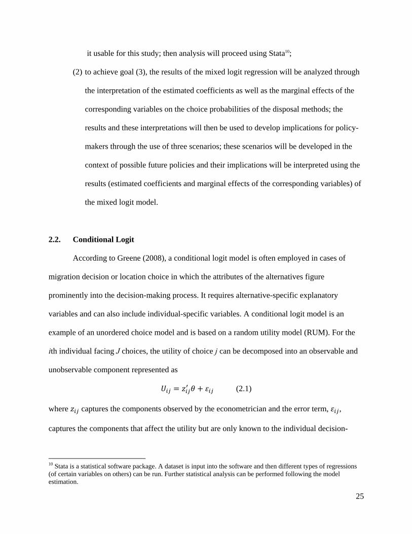
25
it usable for this study; then analysis will proceed using Stata10;
(2) to achieve goal (3), the results of the mixed logit regression will be analyzed through
the interpretation of the estimated coefficients as well as the marginal effects of the
corresponding variables on the choice probabilities of the disposal methods; the
results and these interpretations will then be used to develop implications for policy-
makers through the use of three scenarios; these scenarios will be developed in the
context of possible future policies and their implications will be interpreted using the
results (estimated coefficients and marginal effects of the corresponding variables) of
the mixed logit model.
2.2. Conditional Logit
According to Greene (2008), a conditional logit model is often employed in cases of
migration decision or location choice in which the attributes of the alternatives figure
prominently into the decision-making process. It requires alternative-specific explanatory
variables and can also include individual-specific variables. A conditional logit model is an
example of an unordered choice model and is based on a random utility model (RUM). For the
ith individual facing J choices, the utility of choice j can be decomposed into an observable and
unobservable component represented as
(2.1)
where captures the components observed by the econometrician and the error term, ,
captures the components that affect the utility but are only known to the individual decision-
10 Stata is a statistical software package. A dataset is input into the software and then different types of regressions (of certain variables on others) can be run. Further statistical analysis can be performed following the model estimation.
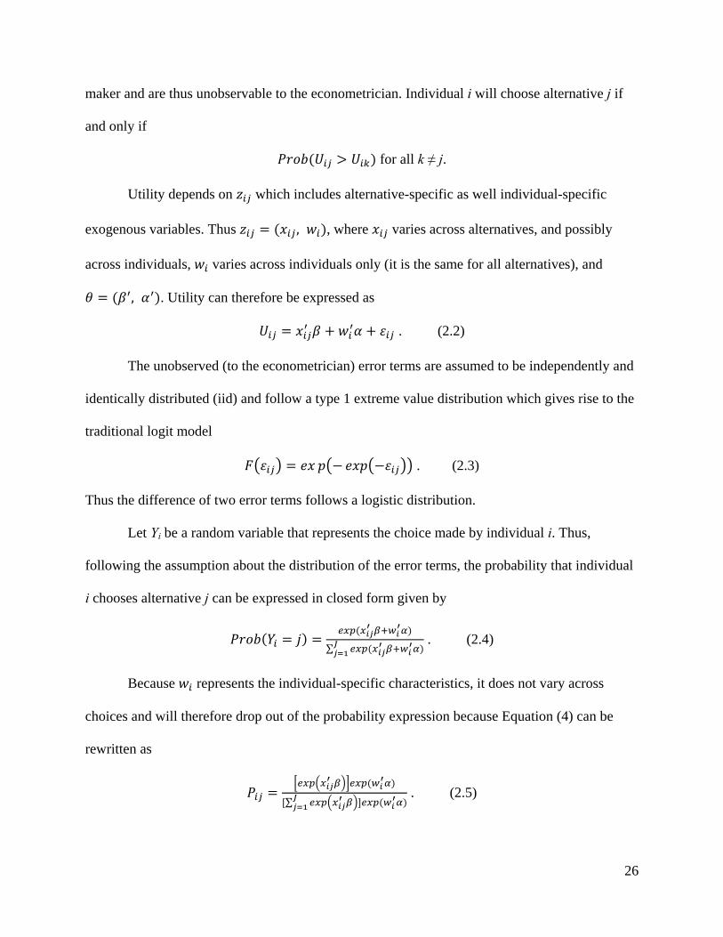
26
maker and are thus unobservable to the econometrician. Individual i will choose alternative j if
and only if
for all k ≠ j.
Utility depends on which includes alternative-specific as well individual-specific
exogenous variables. Thus , , where varies across alternatives, and possibly
across individuals, varies across individuals only (it is the same for all alternatives), and
, . Utility can therefore be expressed as
. (2.2)
The unobserved (to the econometrician) error terms are assumed to be independently and
identically distributed (iid) and follow a type 1 extreme value distribution which gives rise to the
traditional logit model
. (2.3)
Thus the difference of two error terms follows a logistic distribution.
Let Yi be a random variable that represents the choice made by individual i. Thus,
following the assumption about the distribution of the error terms, the probability that individual
i chooses alternative j can be expressed in closed form given by
∑ . (2.4)
Because represents the individual-specific characteristics, it does not vary across
choices and will therefore drop out of the probability expression because Equation (4) can be
rewritten as
∑ . (2.5)
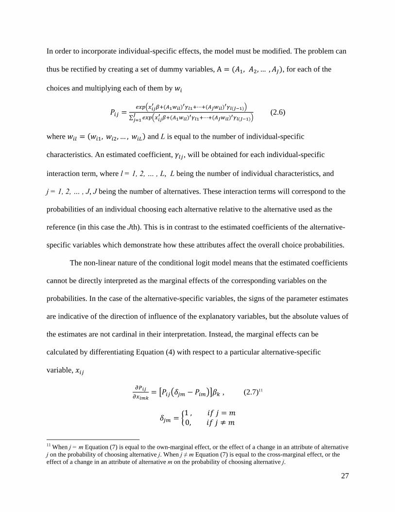
27
In order to incorporate individual-specific effects, the model must be modified. The problem can
thus be rectified by creating a set of dummy variables, A , , …, , for each of the
choices and multiplying each of them by
⋯
∑ ⋯(2.6)
where , , … , and L is equal to the number of individual-specific
characteristics. An estimated coefficient, , will be obtained for each individual-specific
interaction term, where l = 1, 2, … , L, L being the number of individual characteristics, and
j = 1, 2, … , J, J being the number of alternatives. These interaction terms will correspond to the
probabilities of an individual choosing each alternative relative to the alternative used as the
reference (in this case the Jth). This is in contrast to the estimated coefficients of the alternative-
specific variables which demonstrate how these attributes affect the overall choice probabilities.
The non-linear nature of the conditional logit model means that the estimated coefficients
cannot be directly interpreted as the marginal effects of the corresponding variables on the
probabilities. In the case of the alternative-specific variables, the signs of the parameter estimates
are indicative of the direction of influence of the explanatory variables, but the absolute values of
the estimates are not cardinal in their interpretation. Instead, the marginal effects can be
calculated by differentiating Equation (4) with respect to a particular alternative-specific
variable,
, (2.7)11
1, 0,
11 When j = m Equation (7) is equal to the own-marginal effect, or the effect of a change in an attribute of alternative j on the probability of choosing alternative j. When j ≠ m Equation (7) is equal to the cross-marginal effect, or the effect of a change in an attribute of alternative m on the probability of choosing alternative j.
28
where j, m = 1, … , J and k = 1, … , K and represents the kth attribute of alternative m.
The nature of Equation (2.7) indicates that the cross marginal effects of a particular
alternative’s attributes on the probabilities that any of the other alternatives will be chosen
exhibit the opposite sign from the attributes’ own marginal effects on the probability that that
particular alternative will be chosen. This means that if a change in a particular alternative’s
attribute results in an increase in the probability that that alternative will be chosen, that same
change will also result in a decrease in the probabilities that any of the other alternatives will be
chosen. The decrease in the probabilities that any of the other alternatives will be chosen
compensates for the increase in the probability that a particular alternative will be chosen.
The error assumption that gives rise to the conditional logit model requires an
independence of irrelevant alternatives (IIA) assumption. The IIA property means that the ratio
, for all j, k, is constant and is independent of the other remaining probabilities. Thus, if
another alternative is added or if the characteristics of any of the other alternatives are changed
the ratio between the two probabilities in consideration will not change. Additionally, this
assumption precludes the ability to correlate errors across individual drilling operators who may
appear multiple times in the dataset. The assumption of IIA simplifies the estimation process but
is not realistic when applied to real-world situations. There is no reason to think that an
individual decision-maker will not take into account the characteristics of all the alternatives
when making his/her choice. In the case of drilling operators, it is reasonable to assume that each
drilling operator will take into consideration the characteristics of each of the three disposal
methods before deciding which method to utilize. Thus, a mixed logit model will be used to relax
the IIA assumption. This approach will also allow tastes to vary across individuals (drilling
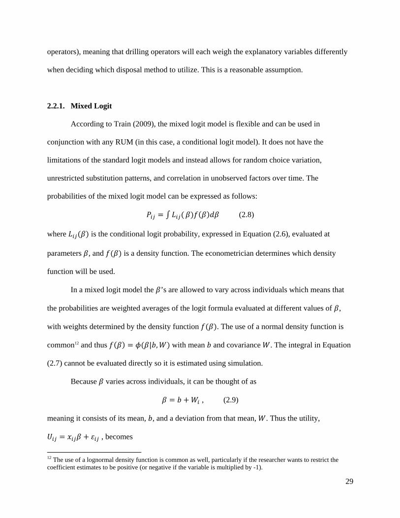
29
operators), meaning that drilling operators will each weigh the explanatory variables differently
when deciding which disposal method to utilize. This is a reasonable assumption.
2.2.1. Mixed Logit
According to Train (2009), the mixed logit model is flexible and can be used in
conjunction with any RUM (in this case, a conditional logit model). It does not have the
limitations of the standard logit models and instead allows for random choice variation,
unrestricted substitution patterns, and correlation in unobserved factors over time. The
probabilities of the mixed logit model can be expressed as follows:
(2.8)
where is the conditional logit probability, expressed in Equation (2.6), evaluated at
parameters , and is a density function. The econometrician determines which density
function will be used.
In a mixed logit model the ’s are allowed to vary across individuals which means that
the probabilities are weighted averages of the logit formula evaluated at different values of ,
with weights determined by the density function . The use of a normal density function is
common12 and thus | , with mean and covariance . The integral in Equation
(2.7) cannot be evaluated directly so it is estimated using simulation.
Because varies across individuals, it can be thought of as
, (2.9)
meaning it consists of its mean, , and a deviation from that mean, . Thus the utility,
, becomes
12 The use of a lognormal density function is common as well, particularly if the researcher wants to restrict the coefficient estimates to be positive (or negative if the variable is multiplied by -1).
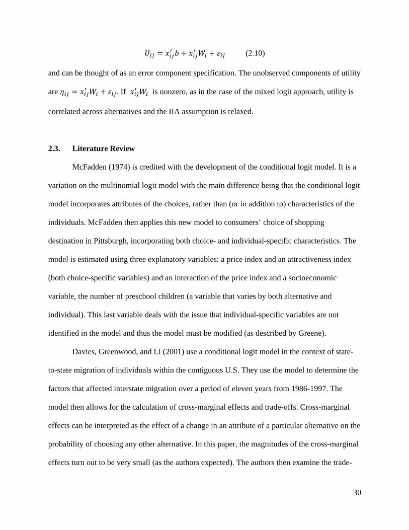
30
(2.10)
and can be thought of as an error component specification. The unobserved components of utility
are . If is nonzero, as in the case of the mixed logit approach, utility is
correlated across alternatives and the IIA assumption is relaxed.
2.3. Literature Review
McFadden (1974) is credited with the development of the conditional logit model. It is a
variation on the multinomial logit model with the main difference being that the conditional logit
model incorporates attributes of the choices, rather than (or in addition to) characteristics of the
individuals. McFadden then applies this new model to consumers’ choice of shopping
destination in Pittsburgh, incorporating both choice- and individual-specific characteristics. The
model is estimated using three explanatory variables: a price index and an attractiveness index
(both choice-specific variables) and an interaction of the price index and a socioeconomic
variable, the number of preschool children (a variable that varies by both alternative and
individual). This last variable deals with the issue that individual-specific variables are not
identified in the model and thus the model must be modified (as described by Greene).
Davies, Greenwood, and Li (2001) use a conditional logit model in the context of state-
to-state migration of individuals within the contiguous U.S. They use the model to determine the
factors that affected interstate migration over a period of eleven years from 1986-1997. The
model then allows for the calculation of cross-marginal effects and trade-offs. Cross-marginal
effects can be interpreted as the effect of a change in an attribute of a particular alternative on the
probability of choosing any other alternative. In this paper, the magnitudes of the cross-marginal
effects turn out to be very small (as the authors expected). The authors then examine the trade-
31
offs between per capita income and several explanatory variables in order to approximate the
dollar value of those trade-offs, ceteris paribus. A one-unit increase in , (in this case per
capita income) must increase by to compensate and hold the probability of choosing
alternative j constant. The trade-off can be equated to the marginal rate of substitution (MRS)
between the two variables in question while holding the utility constant. In this paper, the authors
seek to demonstrate the use of a conditional logit model in studying state-to-state migration of
individuals in particular. They envision that this approach can then be extended to location
choice in general.
O’Keefe (2004) utilizes a county-level conditional logit model to determine the effects
that influence migration of welfare recipients in California. She uses Equation (7) to demonstrate
the relationship between the estimated coefficients and the marginal effects of the explanatory
variables on the probabilities of moving between every pair of counties. The author notes that the
large number of counties means that, for most pairs, the probabilities will generally be very
small. She then divides both sides of Equation (7) by which results in a partial elasticity, the
percentage change in probability as a result of a one-unit change in a particular variable, .
Because is usually small, is an approximation for the partial elasticity. This interpretation
for the estimated coefficients is only valid if it is assumed that the probabilities are very small.
The author then goes on to note that the state of California should be aware of the factors
affecting migration, as presented in her paper, and take current migratory trends into
consideration when designing future welfare policies.
Bayoh, Irwin, and Haab (2006) use a conditional logit model in the context of location
choice. They refer to their model as a “hybrid” conditional logit model because, in addition to
considering the effects of choice-specific attributes (as a traditional conditional logit model
32
does), it also considers the effects of individual-specific characteristics (by interacting the choice
dummy variables with the household-specific variables to ensure that the household-specific
variables are identified in the model). This model is then used to determine the relative effects of
community (choice-specific attributes) versus household characteristics (individual-specific
characteristics) on the determination of residential location choice. Bayoh et al. also note the
need to incorporate a set of dummy interaction terms for each household variable that correspond
to each alternative to ensure that the household variable does not drop out of the model. Because
the nonlinear nature of the conditional logit model means that it will generate estimated
coefficients that are not equal to the marginal effects of the corresponding variable, Bayoh et al.
use the marginal effects, calculated by Equation (7), to compute partial elasticities, the effect of a
one-percent change in a particular variable, , on the probability that a household will choose
one of the locations. The authors go on to conclude that household location decisions are most
influenced by community attributes (alternative-specific variables) associated with a “flight-
from-blight” process of suburbanization rather than one of natural evolution (largely due to
changes in individual-specific variables). These results indicate that local policies could be used
to increase the attractiveness of city attributes to encourage in-migration and discourage out-
migration in order to revitalize city centers.
It is also common for a conditional logit model to be used in the case of brand choice
because price, along with health and safety indices (alternative-specific variables), figure
prominently into an individual’s choice of which brand to purchase. Batte et al. use a conditional
logit model to examine customers’ willingness to pay for different levels (100%, 95%, 70%) of
organic content in breakfast cereals. They found that the estimated coefficient on the price
variable was significant and negative as expected, suggesting that as the price of the organic
33
product rises relative to the price of the conventional one, the customer will be less likely to
purchase the organic product. They also found that the estimated coefficient on the food safety
index was significant and positive, suggesting that customers are more likely to purchase organic
products over conventional ones to avoid pesticides and genetically modified organisms
(GMOs). Individual-specific variables, such as income, race, and number of children in the
household, were also included in the model. The authors then used the results of the conditional
logit model to estimate customers’ willingness to pay for organic products. They found that
nutritional and food safety concerns were the primary motivators for purchasing organic
products, outweighing the higher prices of these products. The results of their contingent
valuation experiment suggested that changes in price do not significantly affect the probability of
choosing an organic product. This suggests that customers are willing to pay a premium price for
organic products in order to protect their health.
The use of a conditional logit model is also common in cases of recreation demand
choice. As described by Train (1998), a prominent example is the application of a conditional
logit model to fishing, in which anglers must decide whether to take a fishing trip during a
specified period, which species of fish to target, and/or which fishing site to travel to. The nature
of the conditional logit model allows characteristics of the alternatives (e.g. the time and cost of
traveling to the site, the catch rate, the availability of campgrounds, etc.) as well as
characteristics of the individual anglers (e.g. age, sex, and income, etc.) to be considered. As
mentioned above in the case of the choice of organic vs. conventional cereal, the results of the
conditional logit model are then used to estimate the anglers’ willingness to pay for changes in
site attributes. Train recognizes the limitations of the IIA assumption of the conditional logit
model and instead utilizes a mixed logit model that allows the estimated coefficients to vary over
34
individuals to account for taste differences across individuals. This also implies that the
unobserved component of utility associated with any alternative is correlated over time for each
individual. This property is included in the estimation when an individual encounters more than
one choice situation within the data set.
Hynes and Hanley (2005) use a mixed logit model to examine taste heterogeneity in
kayakers’ choice of whitewater site. They discuss their attempted use of a lognormal density
function for some of the coefficients. A lognormal density function is used if the researcher
wants to restrict the coefficient estimates to be positive (or negative if the variable is multiplied
by -1). The authors expected the trip cost coefficient to be negative for all kayakers in order for
the model to exhibit rational behavior because one would expect that as the trip cost increased a
kayaker would be less likely to visit that site. They also expected the scenery and water quality
coefficients to be positive as one would expect that kayakers would prefer better quality scenery
and water, not worse. However they found that using a lognormal density function did not allow
the mixed logit model to converge. They go on to say that Brownstone and Train encountered
this same problem in one of their papers. Thus Hynes and Hanley use a normal density function
for all of the coefficients in the model.
Christiadi and Cushing (2007) discuss the use of a conditional logit model in the context
of migration. Very early on in the paper the authors bring up the issue of the IIA assumption and
say a violation of this assumption could lead to an incorrect prediction of the probability of
different migration destinations being chosen. They use this concern as a stepping stone in their
paper and devote its remainder to discussing other models that have been developed to relax the
IIA assumption, including the mixed logit model. The authors go on to say that when they ran
the conditional logit model with their data it only took a little over a minute to complete the
35
regression whereas the mixed logit model took nearly 10 hours. Thus relaxing the IIA
assumption necessarily results in significant time and computational costs. But on the positive
side, the more complex mixed logit model results in a more efficient estimation and thus a higher
likelihood value. They also found that, for the most part, the corresponding estimated
coefficients in both the mixed and conditional logit models were of the same sign and statistical
significance, but the magnitudes of the estimated coefficients in the mixed logit model were
consistently higher. The authors conclude, as did Dahlberg and Eklof in one of their papers, that
the mixed and conditional logit models are qualitatively very similar. Thus, the results of a
conditional logit model can often be used as a general approximation of models, such as the
mixed logit model, that relax the IIA assumption. They point out that if it is the researcher’s goal
to merely discover the individuals’ average preferences, a violation of the IIA assumption of the
conditional logit model is not of much concern. But if it is the researcher’s goal to more
accurately forecast the substitution patterns among alternatives due to changes in their
characteristics, it is important to utilize a model that relaxes the IIA assumption, such as a mixed
logit model.
Choi and Ishii (2010) estimate both a conditional logit model and a mixed logit model to
examine the degree to which consumers’ perception of a manufacturer’s warranty is a signal of
unobservable car quality. When comparing the two models, the authors found, as Christiadi and
Cushing did, that they are qualitatively similar. They then conclude that the differences between
the two models, namely the counterintuitive coefficients estimated by the conditional logit
model, might be a byproduct of the restrictive IIA assumption. The authors go on to calculate the
marginal effects of each of the exogenous variables on the choice probabilities. The basic
equation is the same as Equation (2.7) but the authors modify it a bit. Instead of calculating the
36
marginal effects of a “representative” individual, the average of the marginal effects of all the
individuals is calculated as follows
∑ ∑ 1 (2.11)
where j is the product chosen by individual i, is the estimated probability that consumer i
chooses product j, and is the mean of the estimated coefficient of . It makes sense to
calculate the average of the marginal effects because the mixed logit estimation results report the
mean of the estimated coefficients (in the mixed logit model the coefficient estimates vary across
individuals).
Arik Levinson (1996) uses a conditional logit model to examine the effect of differences
in the stringency of state environmental regulations on the location choice of manufacturers. One
of the issues he faces is quantifying the regulations in a significant way. There are currently three
broad categories of ways in which to quantify these regulations: qualitative indicators of
regulatory stringency, quantitative measures of the states’ enforcement efforts, and quantitative
measures of the manufacturing plants’ compliance costs. Levinson develops and explores six
environmental regulatory measures that fall into these three categories. He then uses a
conditional logit model to determine the probability that a particular state maximizes profits for a
particular plant. To overcome the IIA issue, regional dummy variables are included for the four
Census regions explored in this study. The author found that environmental regulations do not
significantly affect the opening of new manufacturing plants. The main implications of this
particular article are the ways in which the environmental regulations can be quantified and
applied within a conditional logit setting.
37
3. Data
3.1. Description
The data used in this thesis are sourced from the PA DEP Oil & Gas Reporting Website
(https://www.paoilandgasreporting.state.pa.us/publicreports/Modules/Welcome/
Welcome.aspx). This website allows the public to view oil and gas well production and waste
data dating back to the year 2000. This information is reported to the PA DEP and then made
publicly available in accordance with Pennsylvania law. An amendment to the 1984 Oil and Gas
Act, signed into law on March 22, 2010, requires drilling operators to file semi-annual
production data reports with the PA DEP on or before February 15th and August 15th of each
year that include the data from the previous six-month period. Under the original act, the
production data remained proprietary for five years, but under the amended act the PA DEP is
required to make the reports publicly available on its website after six months (Oil & Gas Act of
2010, P.L. 169, No. 15). The law does not specifically mention the provision of waste data, but it
is also included in the reports.
The “Marcellus Only” waste report for the period July-December 2011 was downloaded
on May 23, 2012, for use in this thesis. Appendix A details how the data in the waste report was
prepared and cleaned for use in this thesis. The report includes information such as gas
production well location, operating company name, waste type (i.e. basic sediment, brine, drill
cuttings, drilling, flowback fracturing sand, frac fluid, spent lubricant), disposal method (i.e.
brine or industrial waste treatment plant, injection disposal well, landfill, municipal sewage
treatment plant, reuse other than road spreading), waste quantity, waste facility name, and waste
facility location. Because this thesis is only concerned with wastewater, the dataset is limited to
38
the “brine” and “frac fluid” waste types. “Brine” refers to produced water, or the water that will
return to the surface over the life of a producing well. “Frac fluid” refers to flowback water, or
the water that will return to the surface immediately after fracing is completed.
One of the “Disposal Method” classifications is “Reuse Other Than Road Spreading” and
includes both recycling and on-site treatment and reuse or dilution and reuse. The observations
that include a Waste Facility Permit Number and/or an address can be identified as dedicated
recycling facilities. The other observations are labeled as “Frac Water Reuse”, “Reuse of Brine
to Frac a Well”, “Reused for UIC Class II”, or “Reused in Drilling or Plugging Job” but they
cannot be positively identified as either on-site treatment and reuse or dilution and reuse (the
labels are not descriptive enough) (Yoxtheimer)13. For this reason, those observations that are not
identified as dedicated recycling facilities will be excluded from the data set.
The “Disposal Method” classification “Landfill” will be excluded from the data set
because it is not technically (liquid) wastewater that is being disposed of in these facilities; the
wastewater is solidified first before it is disposed of in landfills. The “Disposal Method”
classification “Municipal Sewage Treatment Plant” will also be excluded from the data set.
Firstly there are only four such observations, totaling only 408 bbls. And secondly, because of
the PA DEP’s request for drilling operators to stop sending wastewater to municipal sewage
treatment plants, this disposal method will not be a viable option in the future (the 408 bbls that
were disposed of this way in the second half of 2011 were most likely residuals from before the
PA DEP’s request).
After excluding the necessary observations from the original data set, the wastewater
volume totals are as described in Table 3.1 (an amendment of Table 1.2). The recycling and
13 David Yoxtheimer, of the Penn State Marcellus Center for Outreach and Research, offered guidance in the deciphering of the different labels applied to the “Reuse Other Than Road Spreading” classification.
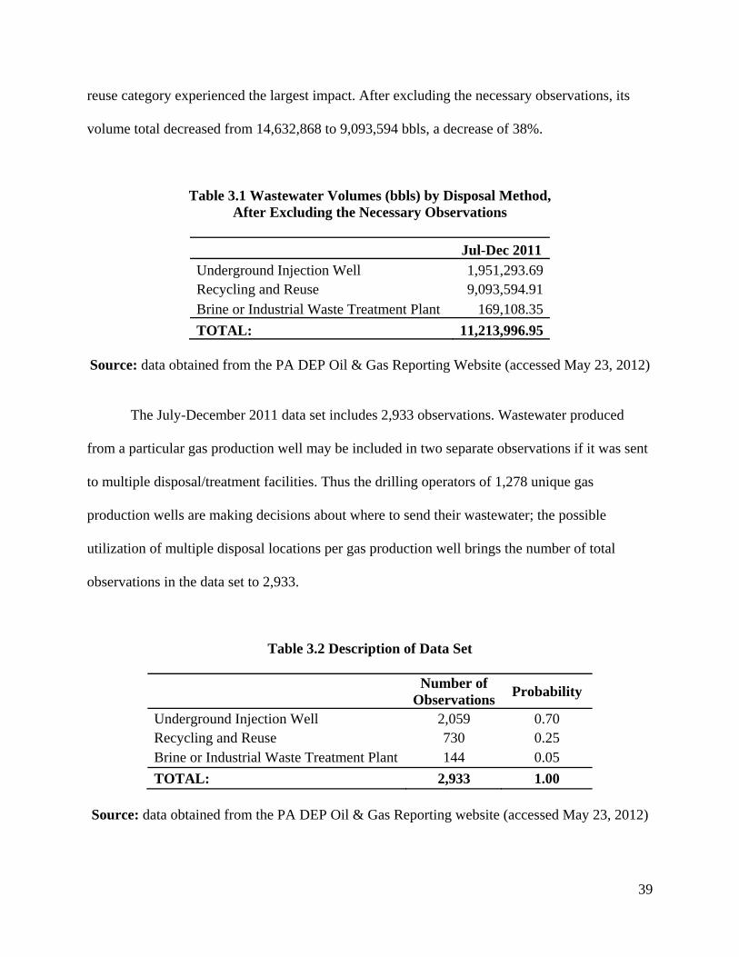
39
reuse category experienced the largest impact. After excluding the necessary observations, its
volume total decreased from 14,632,868 to 9,093,594 bbls, a decrease of 38%.
Table 3.1 Wastewater Volumes (bbls) by Disposal Method, After Excluding the Necessary Observations
Jul-Dec 2011
Underground Injection Well 1,951,293.69 Recycling and Reuse 9,093,594.91 Brine or Industrial Waste Treatment Plant 169,108.35
TOTAL: 11,213,996.95
Source: data obtained from the PA DEP Oil & Gas Reporting Website (accessed May 23, 2012)
The July-December 2011 data set includes 2,933 observations. Wastewater produced
from a particular gas production well may be included in two separate observations if it was sent
to multiple disposal/treatment facilities. Thus the drilling operators of 1,278 unique gas
production wells are making decisions about where to send their wastewater; the possible
utilization of multiple disposal locations per gas production well brings the number of total
observations in the data set to 2,933.
Table 3.2 Description of Data Set
Number of
ObservationsProbability
Underground Injection Well 2,059 0.70 Recycling and Reuse 730 0.25 Brine or Industrial Waste Treatment Plant 144 0.05
TOTAL: 2,933 1.00 Source: data obtained from the PA DEP Oil & Gas Reporting website (accessed May 23, 2012)
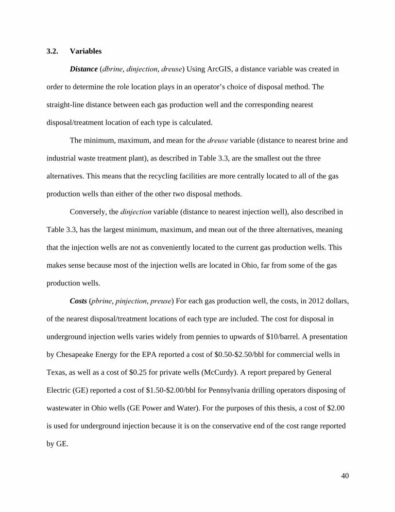
40
3.2. Variables
Distance (dbrine, dinjection, dreuse) Using ArcGIS, a distance variable was created in
order to determine the role location plays in an operator’s choice of disposal method. The
straight-line distance between each gas production well and the corresponding nearest
disposal/treatment location of each type is calculated.
The minimum, maximum, and mean for the dreuse variable (distance to nearest brine and
industrial waste treatment plant), as described in Table 3.3, are the smallest out the three
alternatives. This means that the recycling facilities are more centrally located to all of the gas
production wells than either of the other two disposal methods.
Conversely, the dinjection variable (distance to nearest injection well), also described in
Table 3.3, has the largest minimum, maximum, and mean out of the three alternatives, meaning
that the injection wells are not as conveniently located to the current gas production wells. This
makes sense because most of the injection wells are located in Ohio, far from some of the gas
production wells.
Costs (pbrine, pinjection, preuse) For each gas production well, the costs, in 2012 dollars,
of the nearest disposal/treatment locations of each type are included. The cost for disposal in
underground injection wells varies widely from pennies to upwards of $10/barrel. A presentation
by Chesapeake Energy for the EPA reported a cost of $0.50-$2.50/bbl for commercial wells in
Texas, as well as a cost of $0.25 for private wells (McCurdy). A report prepared by General
Electric (GE) reported a cost of $1.50-$2.00/bbl for Pennsylvania drilling operators disposing of
wastewater in Ohio wells (GE Power and Water). For the purposes of this thesis, a cost of $2.00
is used for underground injection because it is on the conservative end of the cost range reported
by GE.
41
For wastewater exported from Pennsylvania to Ohio, an additional disposal fee of
$0.20/bbl is added to the cost. The passage of Ohio’s Senate Bill 165 in 2010 made some
changes to the state’s UIC program, including an additional disposal fee. The fee amounts to
$0.05/bbl for wastewater originating in-district (within one of the three districts in which an Oil
& Gas regional office is located) and $0.20/bbl for wastewater originating out-of-district
(effectively meaning out-of-state). The fees are collected by the ODNR and are used to run the
Division of Oil and Gas Resources Management (Tomastik).
Three of the four Pennsylvania underground injection wells utilized are private wells14.
Using the estimate from Chesapeake Energy’s report, a private-well cost of $0.25/bbl is used for
the purposes of this thesis (McCurdy). The fourth Pennsylvania injection well is technically a
commercial well15 but the only drilling operator that sent wastewater to the well is the same
company that operates the injection well, effectively making this well a private one for the
purposes of this thesis. Thus, in this case, a cost of $0.25 will also be used (Platt).
According to Quay Shappell, the Chief Operating Officer of TerrAqua Resource
Management, one of the main reasons recycling costs vary across Pennsylvania is the lack of
consensus among the drilling operators as to the water quality standards for beneficial reuse.
Because wastewater that is recycled at dedicated facilities is then sent back out into the field for
reuse at other drilling sites, the drilling operators can determine the water quality treatment
standards that need to be met by the recycling facilities. The prices charged by these facilities are
related to the quality of both the wastewater input and the freshwater output and it is thus
14 As mentioned in Section 1.3.1., private wells are operated by the same drilling company whose production wells produce the wastewater that is disposed of in these wells; they are only permitted to accept wastewater from their own production wells. 15 As mentioned in Section 1.3.1., commercial wells are permitted to accept wastewater originating from any drilling company. They are able to set their own disposal fees.
42
difficult to make a generalization about the cost. If a company only wants the solids removed
from its wastewater it costs less than $2/bbl. On the other hand, if a company wants almost all of
the barium, a scale-forming element, removed it costs upwards of $6-$7/bbl. Now, on average,
companies want the incidence of barium to be reduced from 6,000 to 3,000 parts per million
(ppm) and for this they are charged $4.62/bbl (Shappell). The University of Pittsburgh Graduate
School of Business economic impact study reports a cost of $3.50-$5.50/bbl and Reserved
Environmental Services (RES) reports a cost of $3-$5.50/bbl (Hefley 2011; Kasey). Thus, for the
purposes of this thesis, the cost of $4.62/bbl reported by Shappell will be used, as it also falls
within the other reported ranges.
Treatment and disposal at brine or industrial waste treatment plants costs between $0.12
and $0.25/gallon, or $5.04 and $10.50/bbl (Abdalla et al. 2011). For the purposes of this thesis, a
cost of $6.00/bbl is used (about $0.14/gallon)16.
Size of Drilling Company (size) The number of unique gas production wells operated by
a particular drilling company is used as a proxy for the size of the company. There are 22
companies that operate less than 10 wells, 16 that operate between 10 and 100 wells, and 6
companies that operate more than 100 wells. Thus, of the 44 companies represented in this
dataset, 22 of them, or 50 percent, are small companies operating less than 10 wells. Range
Resources Appalachia LLC is currently the largest drilling operator with 350 gas production
wells across Pennsylvania. The other large companies are Talisman Energy USA Inc. with 268
wells, Chesapeake Appalachia LLC with 248 wells, Atlas Resources LLC with 207 wells,
Chevron Appalachia LLC with 110 wells, and EQT Production Co. with 106 wells.
16 The DEP’s new TDS regulations (500 mg/L, instituted in 2010) apply only to new or expanded TDS loads at facilities accepting wastewater. If they don’t have to adhere to standards that are as stringent, they won’t have to charge prices that are as high (Abdalla et al. 2011). Further research of the websites for the facilities included in the data set indicates that the facilities have been operating at their current levels for some time. Thus a lower price is used.
43
Competition (comp) For each of the gas production wells, a count of the number of other
gas production wells within a 10-mile radius that utilize the same disposal method is used as a
measure of competition.
Distance to Nearest “Large” City (citydist) In order to determine if a gas production
well’s proximity to a city has an impact on the disposal method chosen, a variable is included
that indicates the distance to the closest “large” city/village/municipality/borough. In this case, a
“large” city is any with a population greater than 10,000 people. This data was obtained from the
U.S. Census Bureau’s population estimates, released on June 28, 2012, for the period April 1,
2010 through July 1, 2011. With the exception of the cluster of wells located in the southwest of
Pennsylvania near several “large” cities, including Pittsburgh, most gas production wells seem to
be located in more rural areas of lower population.
A map of the location of these “large” cities can be found in Appendix B.
River Basin (RB) A dummy variable is included to indicate in which river basin a
particular gas production well is located. There are eight river basins in Pennsylvania –
Allegheny, Delaware, Erie, Genesee, Monongahela, Ohio, Potomac, and Susquehanna. The gas
production wells are located in four of them – Allegheny, Monongahela, Ohio, and Susquehanna
– and are pretty evenly distributed among them.
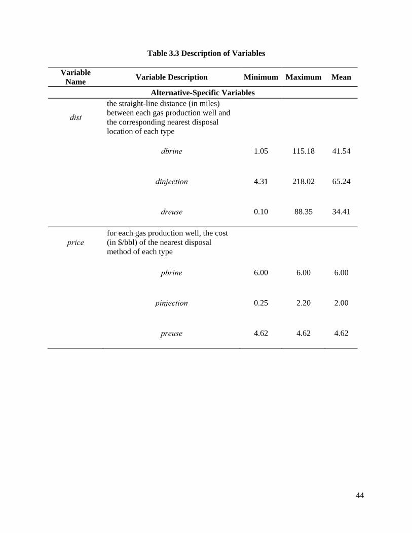
44
Table 3.3 Description of Variables
Variable Name
Variable Description Minimum Maximum Mean
Alternative-Specific Variables
dist
the straight-line distance (in miles) between each gas production well and the corresponding nearest disposal location of each type
dbrine 1.05 115.18 41.54
dinjection 4.31 218.02 65.24
dreuse 0.10 88.35 34.41
price for each gas production well, the cost (in $/bbl) of the nearest disposal method of each type
pbrine 6.00 6.00 6.00
pinjection 0.25 2.20 2.00
preuse 4.62 4.62 4.62
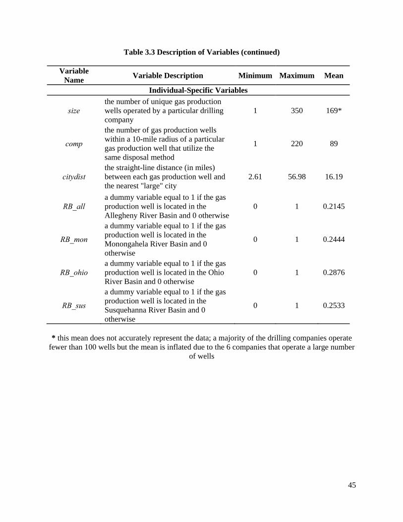
45
Table 3.3 Description of Variables (continued)
Variable Name
Variable Description Minimum Maximum Mean
Individual-Specific Variables
size the number of unique gas production wells operated by a particular drilling company
1 350 169*
comp
the number of gas production wells within a 10-mile radius of a particular gas production well that utilize the same disposal method
1 220 89
citydist the straight-line distance (in miles) between each gas production well and the nearest "large" city
2.61 56.98 16.19
RB_all a dummy variable equal to 1 if the gas production well is located in the Allegheny River Basin and 0 otherwise
0 1 0.2145
RB_mon
a dummy variable equal to 1 if the gas production well is located in the Monongahela River Basin and 0 otherwise
0 1 0.2444
RB_ohio a dummy variable equal to 1 if the gas production well is located in the Ohio River Basin and 0 otherwise
0 1 0.2876
RB_sus
a dummy variable equal to 1 if the gas production well is located in the Susquehanna River Basin and 0 otherwise
0 1 0.2533
* this mean does not accurately represent the data; a majority of the drilling companies operate
fewer than 100 wells but the mean is inflated due to the 6 companies that operate a large number of wells
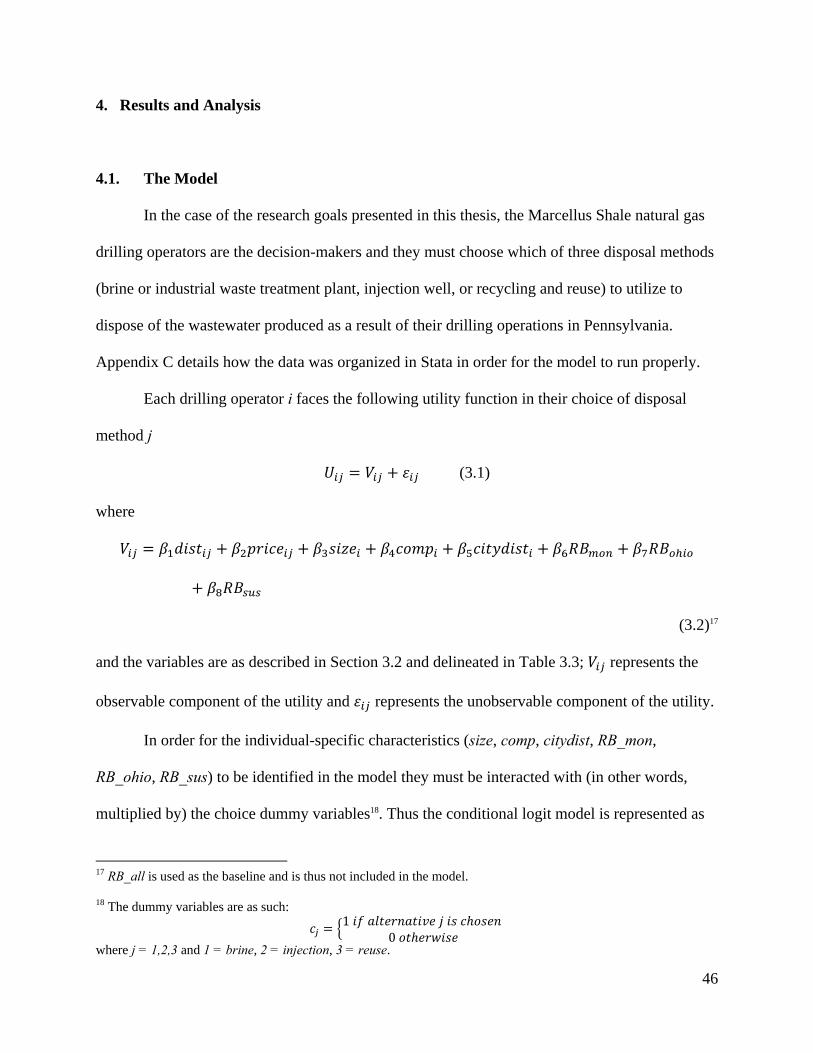
46
4. Results and Analysis
4.1. The Model
In the case of the research goals presented in this thesis, the Marcellus Shale natural gas
drilling operators are the decision-makers and they must choose which of three disposal methods
(brine or industrial waste treatment plant, injection well, or recycling and reuse) to utilize to
dispose of the wastewater produced as a result of their drilling operations in Pennsylvania.
Appendix C details how the data was organized in Stata in order for the model to run properly.
Each drilling operator i faces the following utility function in their choice of disposal
method j
(3.1)
where
(3.2)17
and the variables are as described in Section 3.2 and delineated in Table 3.3; represents the
observable component of the utility and represents the unobservable component of the utility.
In order for the individual-specific characteristics (size, comp, citydist, RB_mon,
RB_ohio, RB_sus) to be identified in the model they must be interacted with (in other words,
multiplied by) the choice dummy variables18. Thus the conditional logit model is represented as
17 RB_all is used as the baseline and is thus not included in the model. 18 The dummy variables are as such:
1 0
where j = 1,2,3 and 1 = brine, 2 = injection, 3 = reuse.
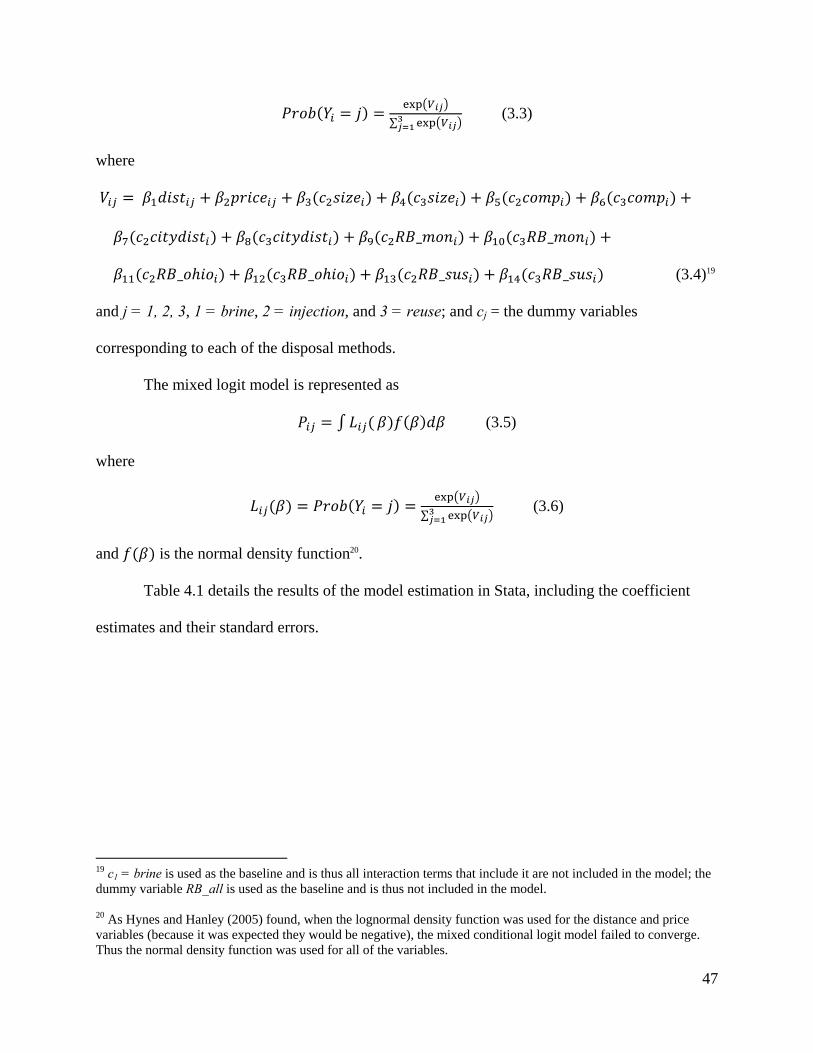
47
∑ (3.3)
where
_ _
_ _ _ _ (3.4)19
and j = 1, 2, 3, 1 = brine, 2 = injection, and 3 = reuse; and cj = the dummy variables
corresponding to each of the disposal methods.
The mixed logit model is represented as
(3.5)
where
∑ (3.6)
and is the normal density function20.
Table 4.1 details the results of the model estimation in Stata, including the coefficient
estimates and their standard errors.
19 c1 = brine is used as the baseline and is thus all interaction terms that include it are not included in the model; the dummy variable RB_all is used as the baseline and is thus not included in the model. 20 As Hynes and Hanley (2005) found, when the lognormal density function was used for the distance and price variables (because it was expected they would be negative), the mixed conditional logit model failed to converge. Thus the normal density function was used for all of the variables.
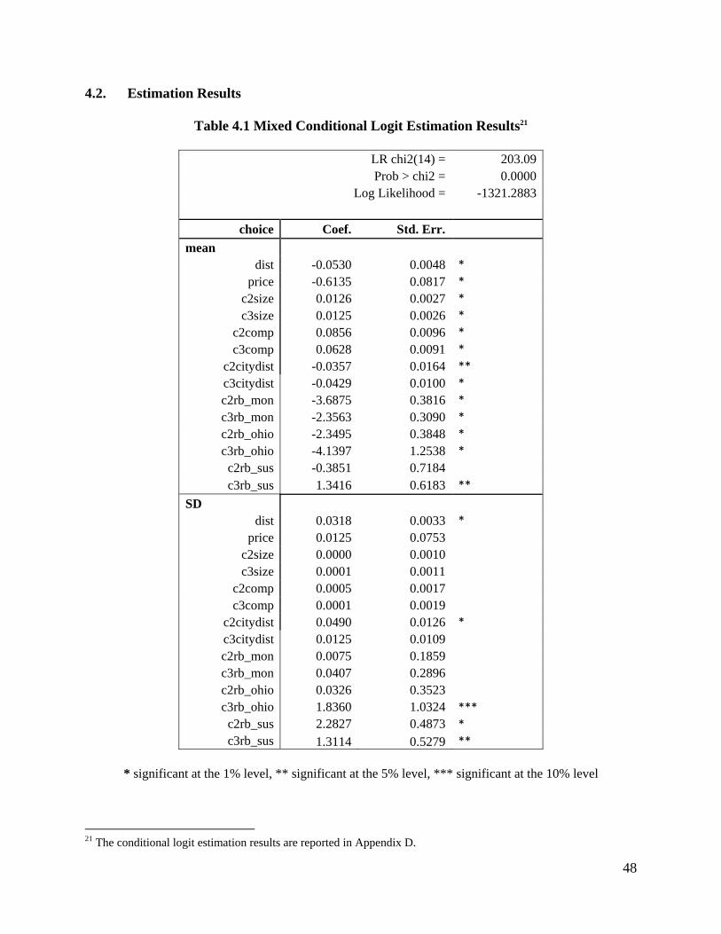
48
4.2. Estimation Results
Table 4.1 Mixed Conditional Logit Estimation Results21
LR chi2(14) = 203.09 Prob > chi2 = 0.0000
Log Likelihood = -1321.2883
choice Coef. Std. Err.
mean
dist -0.0530 0.0048 *
price -0.6135 0.0817 *
c2size 0.0126 0.0027 *
c3size 0.0125 0.0026 *
c2comp 0.0856 0.0096 *
c3comp 0.0628 0.0091 *
c2citydist -0.0357 0.0164 **
c3citydist -0.0429 0.0100 *
c2rb_mon -3.6875 0.3816 *
c3rb_mon -2.3563 0.3090 *
c2rb_ohio -2.3495 0.3848 *
c3rb_ohio -4.1397 1.2538 *
c2rb_sus -0.3851 0.7184
c3rb_sus 1.3416 0.6183 **
SD
dist 0.0318 0.0033 *
price 0.0125 0.0753
c2size 0.0000 0.0010
c3size 0.0001 0.0011
c2comp 0.0005 0.0017
c3comp 0.0001 0.0019
c2citydist 0.0490 0.0126 *
c3citydist 0.0125 0.0109
c2rb_mon 0.0075 0.1859
c3rb_mon 0.0407 0.2896
c2rb_ohio 0.0326 0.3523
c3rb_ohio 1.8360 1.0324 ***
c2rb_sus 2.2827 0.4873 *
c3rb_sus 1.3114 0.5279 **
* significant at the 1% level, ** significant at the 5% level, *** significant at the 10% level
21 The conditional logit estimation results are reported in Appendix D.
49
4.3. Marginal Effects
As mentioned in Section 2.2, the signs of the estimated coefficients indicate the direction
of impact of the corresponding variables, but the absolute values of the estimates are not
indicative of the magnitude of the impact. In order to determine the magnitude, the marginal
effects must be calculated; Equation (2.12) is used to do so. As done by Christiadi and Cushing
(2007), the average marginal effect is calculated for each variable (because the mixed logit
approach calculates the mean of the coefficient estimates).
Table 4.2 details the marginal effect of each explanatory variable. As mentioned in
Section 2.2, the marginal effects of the alternative-specific variables will indicate the direction
and size of the impact of each variable on the overall choice probabilities (regardless of which
alternative is chosen). But the marginal effects of the interaction terms (the individual-specific
variables multiplied by the alternative dummy variables) indicate the direction and size of the
impact of each of the interaction terms on the probability of choosing the corresponding
alternative relative to the alternative used as the baseline (in this case, brine is used as the
baseline).
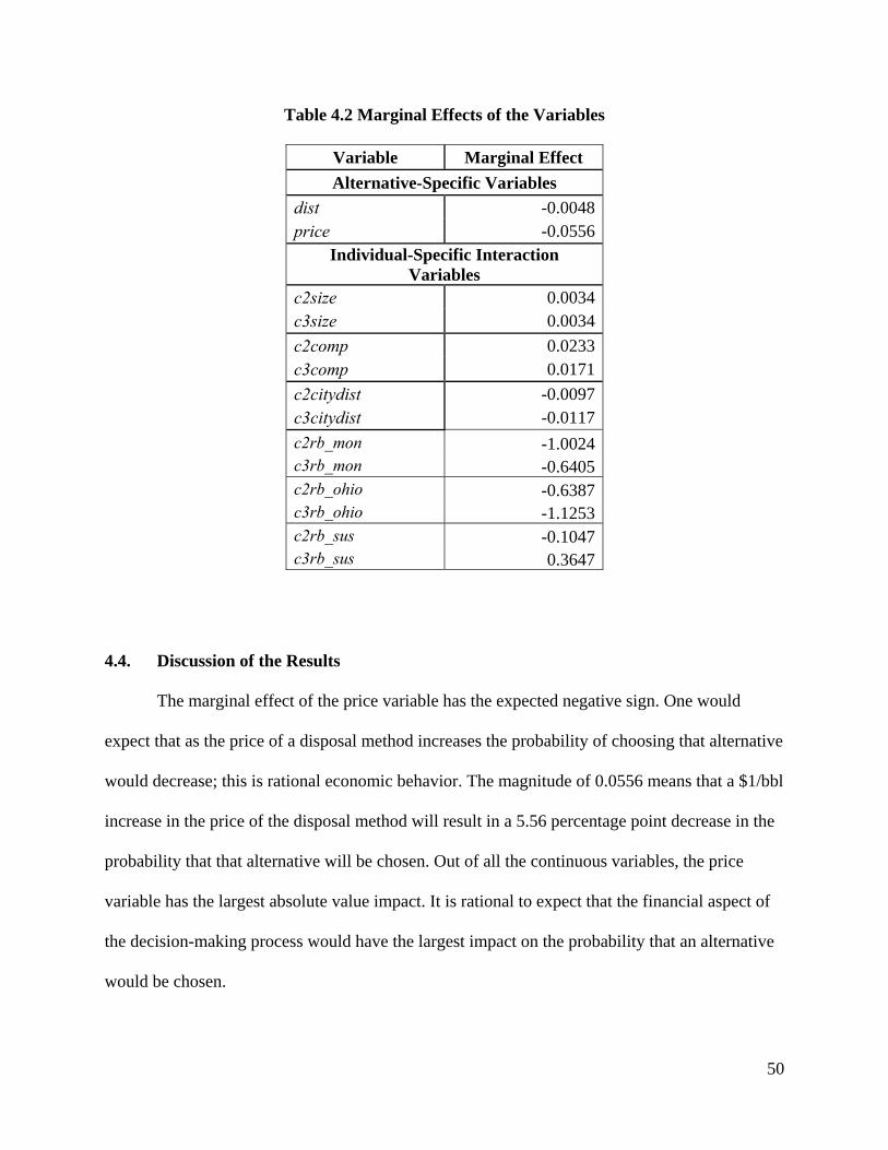
50
Table 4.2 Marginal Effects of the Variables
Variable Marginal Effect
Alternative-Specific Variables
dist -0.0048price -0.0556
Individual-Specific Interaction Variables
c2size 0.0034c3size 0.0034
c2comp 0.0233c3comp 0.0171
c2citydist -0.0097c3citydist -0.0117
c2rb_mon -1.0024c3rb_mon -0.6405c2rb_ohio -0.6387c3rb_ohio -1.1253c2rb_sus -0.1047c3rb_sus 0.3647
4.4. Discussion of the Results
The marginal effect of the price variable has the expected negative sign. One would
expect that as the price of a disposal method increases the probability of choosing that alternative
would decrease; this is rational economic behavior. The magnitude of 0.0556 means that a $1/bbl
increase in the price of the disposal method will result in a 5.56 percentage point decrease in the
probability that that alternative will be chosen. Out of all the continuous variables, the price
variable has the largest absolute value impact. It is rational to expect that the financial aspect of
the decision-making process would have the largest impact on the probability that an alternative
would be chosen.
51
The distance variable also has a marginal effect with a negative sign which is expected.
One would expect that as the distance between the gas production well and the disposal location
increases the probability of choosing an alternative would decrease. The magnitude of the
distance variable is equal to 0.0048, meaning that a one-mile increase in the distance between the
gas production well and the disposal location will result in a 0.48 percentage point decrease in
the probability that that alternative will be chosen.
The distance variable is also tied to the price variable because the distance variable can
be thought of as a proxy for the transportation cost. Thus as the distance between the gas
production well and the disposal location increases the transportation cost also increases. And, as
the sign of the marginal effect of the price variable indicates, as the cost of an alternative
increases the probability of choosing that alternative will decrease. On average, the
transportation cost amounts to about $1/bbl/hr. If it is assumed that the trucks transporting the
wastewater travel, on average, approximately 45 mph22, a distance increase of 45 miles will
result in a $1/bbl increase in transportation costs. The magnitude of the coefficient of the
distance variable indicates that a one-mile increase in distance will result in a 0.48 percentage
point decrease in probability, and thus a 45-mile increase in distance will result in an
approximately 22 percentage point decrease in probability. By extension a $1/bbl increase in
transportation costs (equivalent to a 45-mile increase in distance), will also result in a 22
percentage point decrease in the probability that an alternative will be chosen. Thus, an increase
in the transportation cost will have a larger magnitude of impact (22 percentage points) on the
22 While wastewater disposal trucks can most likely average 60 mph on the interstate highways, many of the production wells are located a considerable distance from the interstates and thus must be accessed by smaller, back roads that require the trucks to travel at lower speeds, closer to 30 mph. Thus, the trucks were estimated to travel at an average of 45 mph.
52
probability of choosing an particular disposal method than an increase in the price of the disposal
method itself (6 percentage points).
Both of the marginal effects of the size variables have a positive sign and the magnitudes
indicate that the addition of one more gas production well to a drilling company’s operation
translates into a 0.34 percentage point increase in the probability that either an injection well or
recycling and reuse will be the disposal method chosen, as compared to the effect of an
additional gas production well on the probability that a brine or industrial waste treatment plant
will be the disposal method chosen. The magnitude of impact is very small which indicates that
size is not as important to the drilling operators’ choice of disposal method. The positive impact
of size on the disposal method chosen could have something to do with economies of scale. For
example, if a drilling company is large enough to completely fill the trucks required to transport
the wastewater to the disposal locations its transportation costs will be the lowest possible,
making transportation more economical. The $1/bbl/hr transportation cost was originally
calculated from a more general cost of $100/hr/truck and thus depends on the truck being filled
to capacity. If a drilling company does not produce enough wastewater to completely fill a truck,
their per barrel transportation cost will actually be higher23.
Both of the marginal effects of the competition variables have a positive sign. An
increase in competition (an additional gas production well within a 10-mile radius of a particular
gas production well) will cause a 2.33 percentage point increase in the probability that an
injection well will be the disposal method chosen and a 1.71 percentage point increase in the
23 The per barrel transportation cost could also be higher if the wastewater disposal trucks idle at the drill sites while waiting to be filled up. Tomastik was consulted regarding this issue. He said that there could be a short wait time at the drill pad before collecting the frac fluid. The trucks are connected to a frac tank via a hose that transfers the wastewater into them. On the other hand, at the production pad there is generally no wait time. The trucks collect the brine directly from a tank called a knockout tank. It seems that the wait time isn’t significant enough to affect the per barrel transportation cost to a great degree.
53
probability that recycling and reuse will be the disposal method chosen, as compared to the effect
of an increase in competition on the probability that a brine or industrial waste treatment plant
will be the disposal method chosen. An increase in competition might have a greater impact on
the choice of an injection well for wastewater disposal due to the higher daily/monthly capacity
for some of them as compared to the other disposal methods. There are also 51 injection wells
accepting wastewater, almost five times as many as either of the other alternatives, meaning that
the total capacity of all of the injection wells combined will be much greater than either of the
other alternatives. An increase in competition might have a positive impact on the choice of
recycling and reuse as the disposal method because it will create a market for the treated
wastewater. The process of recycling and reuse means that the treated wastewater will be sent
back out into the field and used to frac other wells. If there is not a market for this treated water,
the recycling and reuse method will no longer be a viable option. In the long run, if demand for
treated wastewater for fracing continues to increase (a possible result of an increase in
competition because of the limitations placed on freshwater withdrawals), recycling facilities
might be able to lower their per barrel prices, further increasing the probability that recycling and
reuse will be the disposal method chosen.
Both of the marginal effects of the “distance to nearest large city” variables have a
negative sign. As the distance to the nearest “large” city increases by one mile, the probability
that an injection well will be the disposal method chosen decreases by 0.97 percentage points and
the probability that recycling and reuse will be the disposal method chosen decreases by 1.17
percentage points, as compared to the effect of an increase in the distance to the nearest “large”
city on the probability that a brine or industrial waste treatment plant will be the disposal method
chosen. This result could indicate the importance of the infrastructure that goes along with
54
proximity to a city in the wastewater disposal process. Cities have access to better and more
roads usable by large volumes of large truck traffic. They also have the resources to potentially
build pipelines and rail lines for the purposes of transporting large volumes of wastewater more
easily over long distances.
Because injection wells are generally located further from more populated areas than are
recycling facilities, one would expect the distance to the nearest “large” city to matter less (have
a smaller magnitude of impact) for injection wells because as gas production wells are located
further from the cities they might be located closer to the injection wells at which they will
dispose of their wastewater. And, as the negative marginal effect of distance indicates, as the
distance between a gas production well and disposal location decreases, the probability of
choosing that disposal location increases. This slight positive effect would possibly cancel out
some of the negative effect of the distance to the nearest large city, meaning the magnitude of
impact of “distance to nearest large city” on the choice of injection well would be less than the
magnitude of impact of “distance to nearest large city” on the choice of recycling and reuse, as
the results indicate. But the marginal effects are pretty close in magnitude indicating that this
possible effect is not likely to be very strong.
All of the coefficients on the river basin dummy variables are negative, except the
coefficient on the interaction between the recycling and reuse alternative and the Susquehanna
River Basin. This means that, as compared to the gas production well not being located in its
current river basin, being located in its current river basin results in a smaller probability of
choosing either an injection well or recycling and reuse, as compared to choosing a brine or
industrial waste treatment plant. The magnitudes of impact are, in general, larger for the
Monongahela and the Ohio River Basins. This would seem to indicate that any regulations
55
governing water withdrawal and discharge (and ultimately reuse) are more stringent in the
Monongahela and Ohio River Basins, but there is no indication that this is the case in actuality.
This could then indicate the existence of other, as of yet unobservable as well as unfavorable
attributes of these river basins. In this case, “unfavorable” refers to the fact that the signs of the
marginal effects of some of the river basin dummies are negative, indicating that being located in
these river basins means that drilling operators are less likely to choose either an injection well or
recycling and reuse as the disposal option.
The ambiguity in the interpretation of the magnitudes of the marginal effects of the river
basin dummies seems to indicate that the river basin boundaries on their own don’t paint a
complete picture. The boundaries of the PA DEP districts, and possibly of Pennsylvania’s
municipalities, could also play a role in the choice of disposal location. Thus the “unobservable”
attributes mentioned above may not truly be unobservable; instead, the issue might simply be
that the study presented in this thesis was not broad enough to include dummy variables for all of
the possibly relevant boundaries.
On the other hand, being located in the Susquehanna River Basin has a positive impact on
the choice of an injection well as the disposal method. The Susquehanna River Basin
Commission (SRBC) is active in regulating water withdrawals and discharges within its
boundaries. Because most of the injection wells are located farther from this river basin, which is
located farther east than the other three river basins, drilling companies might utilize this
disposal method in order to escape the regulations put in place by the SRBC.
The coefficients on the interaction terms between injection well and Monongahela River
Basin and between recycling and reuse and Ohio River Basin are greater than one, which would
mean that the difference in choice probability, as a result of being located in either of those river
56
basins as compared to not, would be greater than 100 percentage points. A change in probability
that is greater than 100 percentage points does not make sense nor is it intuitive. This is an
indication that there might be a problem with the way the marginal effects of the river basin
dummy variables were calculated and interpreted. According to Choi and Ishii (2010), Equation
(2.12) should only be used to calculate the marginal effects of continuous variables. The
marginal effects of binary (dummy) variables should be calculated as the averages of the
differences of the actual estimated probabilities for the observed choices and the counterfactual
estimated probabilities for the observed choices.
An economic counterfactual simulation involves predicting the new estimated
probabilities of choosing the alternatives when a certain variable is changed. According to the
method employed by Choi and Ishii (2010), when a binary variable is involved, a counterfactual
simulation assumes that the value of the binary variable in question is zero. After performing the
counterfactual simulation (by changing the values of the necessary binary variables to zero and
running these new values back through the previously-estimated model), the marginal effect24 of
the binary variable in question can be determined by averaging the actual estimated probabilities
for the observed choices and the estimated probabilities determined by the counterfactual
simulation.
Because a binary variable can only ever equal zero or one, a probability difference
provides a more natural interpretation than a probability derivative. Unfortunately the limitations
of the Stata command “mixlogit” did not allow for the data to be modified and then run back
through the previously-estimated model and thus this kind of analysis could not be performed.
24 For observed choices whose original value of a binary variable is zero, the contribution to the marginal effect will be zero because the actual and counterfactual probabilities will be same (Choi and Ishii 2010).
57
5. Future Scenarios
5.1. Business-as-Usual
Under the “business-as-usual” scenario, natural gas drilling activity in the Marcellus
Shale will continue to increase, along with the amount of wastewater that must be disposed of.
According to Considine (2010), the regulatory policies of the states involved in natural gas
drilling must be considered when discussing the trajectory of its development. Development
prospects in Pennsylvania continue to remain the strongest of the states in the Marcellus or Utica
Shale regions. The signing of Act 13 of 2012 (amending Title 58 of the Pennsylvania
Consolidated Statutes) which provides for an unconventional gas well fee (also known as a
drilling impact fee) could have an effect on future drilling activity though (Act 13). On the other
hand, West Virginia has already imposed a severance tax and faces limited pipeline capacity and
high pipeline construction costs as a result of the mountainous terrain that must be negotiated.
Ohio, while not involved in drilling in the Marcellus Shale to any great extent, looks to become
more involved in drilling in the Utica Shale (Considine 2010).
Currently in New York there exists an effective moratorium on horizontal drilling and
hydraulic fracturing due to the limitations placed on the amount of water that can be used in the
fracing process. But the large potential economic benefits that natural gas drilling could bring to
the state are encouraging legislators to consider withdrawing this moratorium. Governor Andrew
Cuomo has proposed a plan that would limit fracing to several struggling counties along the
Southern Tier of the state, and only if the communities in which it would be used express their
support for this process (Hakim). If the moratorium were to be lifted, these southern New York
counties could expect to experience a substantial level of drilling activity, if the level of activity
58
just south in Pennsylvania is any indication. All of these policies as a whole must be considered
when trying to predict the overall level of natural gas development in the future.
Considine goes on to posit three development scenarios, extending through 2020, based
on the aforementioned policy considerations. Under the low development scenario, Pennsylvania
will drill close to 1,500 wells per year by 2020 and New York will continue to drill no wells as
the moratorium will still be in effect. Under the medium development scenario, Pennsylvania
will drill close to 2,500 wells per year and New York will drill approximately 300 wells per year
by 2020. Under the high development strategy, Pennsylvania will drill close to 3,600 wells per
year and New York will drill approximately 500 wells per year by 2020. Considine states that the
rising importance of natural gas as part of our nation’s energy future (as a way to end
dependence on foreign oil and create domestic jobs) coupled with the vast growth in activity in
the Barnett Shale in Texas, as well as in other shale plays across the country and throughout the
world, indicate that the actual level of development might fall between the medium and high
scenarios, if the moratorium in New York is lifted. On the other hand, if the moratorium in New
York remains, if regulatory and tax policies are imposed, and/or if the price of natural gas
remains low, the actual level of development might fall closer to the low scenario. Because there
are so many factors to consider, it is extremely difficult to predict exactly what will happen
(Considine 2010).
If the wastewater numbers from the last half of 2011 are any indication, the prevalence of
the use of injection wells and recycling and reuse as disposal methods will continue to grow.
From the first half of 2011 to the second half of 2011, the amount of wastewater disposed of in
injection wells increased from 10% of the total to 11%25 and the amount of wastewater disposed
25 While the percentage increase isn’t that great, the volume increase from 866,023 bbl to 1,951,293 bbl indicates an increase in the prevalence of the use of this disposal method.
59
of through recycling and reuse increased from 69% of the total to 87% while the amount of
wastewater disposed of in brine or industrial waste treatment plants decreased from 14% of the
total to 1%. Because it is expected that the level of natural gas drilling will continue to increase,
and, by extension, the amount of wastewater that must be disposed of, there is reason to believe
that this trend in the prevalence of the use of disposal methods will continue in the immediate
future.
Particularly if the moratorium in New York is lifted, a large increase in competition for
wastewater disposal can be expected26. As the marginal effects of the competition variable
indicate, an increase in competition will result in an increase in the probability that an injection
well or recycling and reuse will be the disposal method chosen, as compared to a brine or
industrial waste treatment plant. As mentioned in Section 1.3.1, most of the injection wells
currently in operation, particularly in Pennsylvania, have been in operation since the 1980s and
have still not reached their maximum capacity. They have also not seen very significant and
intense levels of activity to date27. This is an indication that the Pennsylvania underground
injection wells will continue to be able to accept the increasing volumes of wastewater that can
be expected, at least in the short term (Platt; Tomastik). Information gleaned from both Platt and
26 If the moratorium in New York was lifted and the state began drilling, and thus producing wastewater, the wastewater would have to be disposed of somewhere. There is no indication to suggest that New York possesses any major capacity to handle large volumes of wastewater and thus drilling operators in New York would most likely be competing with those in Pennsylvania for the use of disposal methods in the short term (at least during the beginning stages of drilling activity in New York, before it could potentially develop its own disposal/treatment facilities and technologies). 27 As compared to the injection activity that might be expected as drilling activity continues to increase.
60
Tomastik helped to form these assumptions28. Also, there are almost five times as many injection
wells accepting wastewater as either of the other disposal methods, another indication of
sufficient capacity at present.
In the case of recycling and reuse, the effect of competition might be two-fold. An
increase in competition could place a strain on the amount of freshwater available for
withdrawals used in the fracing process. This in turn could create a market for treated water
sourced from recycling facilities to be used in the fracing process instead, therefore encouraging
the use of existing and the development of new recycling and reuse facilities to dispose of/treat
drilling wastewater.
As drilling activity and the volume of wastewater increase, if the state were to further
encourage recycling and reuse as a disposal method29, it could decrease the need for additional
freshwater withdrawals and the amount of wastewater that must be disposed of. This would
increase water use efficiency and help protect Pennsylvania’s environment and waterways.
5.2. Permanent Moratorium in Youngstown, Ohio
As mentioned in 1.3.1, following the twelve earthquakes that occurred in Ohio in 2011,
that have since been linked to an underground injection well in the Youngstown area, state
officials issued a temporary moratorium on all underground injection activity within a five-mile
28 For example, in the short term in Ohio there is also sufficient capacity, but, according to Tomastik, there are currently 29 new permit applications pending, an indication that the high level of drilling activity is putting a strain on current capacity. He believes that in the long term a greater emphasis will be put on the recycling and reuse of wastewater to relieve the strain placed on underground injection capacity (as well as to decrease the amount of freshwater withdrawals needed in the fracing process and to cut down on disposal costs). 29 This could perhaps be accomplished through some sort of subsidy because, as its marginal effect indicates, a decrease in price results in an increase in the probability that the alternative in question will be chosen. Incentives for recycling facilities to be built close to where the production wells are located would be another way to accomplish this because, as the marginal effect of the distance variable (a proxy for the transportation cost) indicates, the transportation cost plays a large role in the probability that a disposal method will be chosen.
61
radius of the injection well in question. Since then a determination has not yet been made as to
the permanency of the moratorium. A permanent moratorium could be a possibility though – one
was put in place in Arkansas following a swarm of earthquakes in the north-central part of the
state that was linked to underground injection.
The way the data is currently defined (the distance variable is defined as the distance
between the gas production well and the nearest disposal location of each type) it is not possible
to model directly the effect of the Youngstown, Ohio, wells being removed from the data set
because none of the Pennsylvania gas production wells have any of the Youngstown wells as
their nearest injection well option. This scenario can be considered by applying the results of the
model estimation and the interpretation of the marginal effects to it, though. The drilling
operators of the 60 Pennsylvania gas production wells that utilize the Youngstown injection
wells will have to reevaluate their disposal method choice. If the next closest injection well is
closer than the Youngstown well, the drilling operator might start using this new injection well.
On the other hand, if the next closest injection well is farther away than the Youngstown well,
the drilling operator might consider utilizing a different disposal method because, as its marginal
effect indicates, an increase in the distance variable will result in a decrease in the probability
that a disposal method will be chosen.
The permanent moratorium will also affect wastewater produced in Ohio. According to
Tomastik, natural gas development in the Utica Shale in Ohio is on track to increase in the
coming years. Ohio anticipates drilling 200 Utica wells in 2012 and even more in the future (they
are at the same stage of development that Pennsylvania was at in 2007 in the Marcellus Shale).
Due to the potential increase in drilling activity in Ohio, and the inevitable increase in
wastewater, Ohio may feel the effects of a permanent moratorium on some of its injection wells
62
in the form of overall reduced injection capacity. As a result, they may feel the need to protect
their supply of injection disposal capacity for their own future use, potentially accomplishing this
by increasing the out-of-district disposal fee (currently set at $0.20/bbl in 2012). If the price of
underground injection in Ohio increases, the probability of Pennsylvania drilling operators
choosing it as a disposal method will decrease, causing drilling operators in Pennsylvania to turn
to disposal methods within-state, including Pennsylvania’s own underground injection wells, or,
more likely, recycling and reuse. Thus a permanent moratorium on underground injection in
Youngstown, Ohio, coupled with an increase in drilling activity in the Utica Shale in Ohio, could
cause an even greater increase in the recycling and reuse of wastewater by drilling operators in
Pennsylvania30, as compared to the current trajectory of this disposal method.
5.3. Pennsylvania Takes Primacy
The increase in drilling activity in the Utica Shale in Ohio could also influence
Pennsylvania’s decision to take primacy of its underground injection program. As mentioned in
Section 1.3.1, an individual state, if it so chooses, can apply to the EPA to obtain primacy, or
primary enforcement responsibility, over its own UIC program, meaning that it would be in
complete control of the program and in charge of overseeing all injection activity and ensuring
that all federal and state requirements were being met (“Underground Injection”). As mentioned
in the previous scenario, an increase in Utica Shale drilling could lead Ohio to attempt to protect
its own supply of injection wells through an increase in the out-of-state disposal fee (currently
set at $0.20/bbl in 2012). An increase in the price of underground injection, as evidenced by the
30 It will be interesting to view the production and waste reports for the first half of 2012 when they are published by the DEP on their Oil & Gas Reporting website on August 15th. The data can be analyzed to determine the effect the temporary moratorium on underground injection has had on the probabilities of choosing each of the three disposal methods.
63
marginal effect of this variable, will lead drilling operators to reevaluate their choice of disposal
method. Because most of Pennsylvania’s injection wells are private facilities, recycling and reuse
would be the natural next choice, but if Pennsylvania wanted to encourage underground injection
within its borders, it would need to obtain primacy of its own program.
Primacy would allow Pennsylvania to permit more wells in a shorter period of time (as
evidenced by how primacy allows Ohio to more efficiently operate its program31). It would also
help if these potential new underground injection wells were located closer to the gas production
wells that utilize them. As the marginal effect of the distance variable indicates, a decrease in the
distance between the gas production well and the disposal location would result in an increase in
the probability that it would be the method chosen. The marginal effect of the distance variable
also indicates the large effect that transportation cost (for which the distance variable is a proxy)
has on the choice of disposal method.
Previous, and now inactive, oil and gas production wells can be converted and used as
new underground injection wells, cutting down on the required construction time. Thus the
injection wells could also be located closer to the gas production wells they serve. This option
comes with its own potential problems, though. Groundwater contamination could occur if the
previous, inactive wells were improperly plugged, but primacy would allow Pennsylvania to
institute its own regulations, more stringent than the federal standards, in order to control for this
potential situation (Tomastik). Pennsylvania taking primacy of its underground injection
program would be a potential solution to an increase in drilling in the Utica Shale in Ohio and
thus Ohio increasing its disposal fee to protect its own supply of underground injection capacity.
31 According to Tomastik, primacy eliminates the many bureaucratic hurdles that are present when the EPA is in charge of administering a state’s UIC program. This allows a state to more efficiently operate their program, including permitting more wells in a shorter period of time.
64
6. Research Limitations
6.1. Data Limitations
As noted in Section 3.1, the “Reuse Other Than Road Spreading” observations labeled as
“Frac Water Reuse”, “Reuse of Brine to Frac a Well”, “Reused for UIC Class II”, or “Reused in
Drilling or Plugging Job” could not be positively identified as either on-site treatment and reuse
or dilution and reuse (the labels are not descriptive enough) and thus those observations were
excluded from the data set. But for future research and analysis, it would be helpful to be able to
make the distinction between on-site treatment and reuse or dilution and reuse (a more
interactive form, as discussed in Section 6.1.1, could help with this). It would be interesting to
examine the determinants of choosing on-site treatment and reuse as a disposal method, in
particular the size of the drilling company. According to a University of Pittsburgh Graduate
School of Business economic impact study, purchasing a mobile wastewater treatment unit can
cost upwards of $4 million and renting it can cost about $80,000 per month, with a $73,000
operating cost (that covers fuel and labor) (Hefley 2011). Probably only larger companies, with
many gas production wells that will benefit from the services of such a unit, would be willing or
able to incur these huge fixed costs.
The data required some clean-up in order for it to be useable for the analysis conducted in
this thesis. This was done as indicated in the following description. In the PA DEP waste report
the drilling operators are required to provide the waste disposal method, but the method often
does not match with the actual facility that is also provided. Many operators mistakenly chose
“Brine or Industrial Waste Treatment Plant” when they should have chosen either “Injection
Disposal Well” or “Reuse Other Than Road Spreading.” The Waste Facility Permit Number was
65
examined in order to correct this error. The permit numbers that take the form xx-xxx-xxxxx are
underground injection wells and those that take the form WMGR119NC001 or
WMGR123NC001 are dedicated recycling facilities. If a Waste Facility Permit Number was not
provided, the names of the waste facilities were examined. If the name itself did not give an
indication as to the type of facility, the descriptions provided by the facilities’ websites were
examined in order to make the distinction (Yoxtheimer)32.
Another data problem was that latitude and longitude coordinates were lacking for some
of the waste facilities in the PA DEP data set. In these cases, if a valid/complete street address
was provided, a geocoding tool was used to convert the address to latitude and longitude
coordinates. If a valid/complete street address was not provided, Christopher Tersine at the PA
DEP and Tom Tomastik at the ODNR provided the missing coordinates.
The PA DEP also does not indicate when it updates the waste reports (other than on
February 15th and August 15th). Apparently it will sometimes update the reports in the interim
period if additional information becomes available (presumably if drilling companies submit new
or updated data after the deadline). It would be helpful to know when and if these updates occur
(i.e. a new version should be created each time an update is made) so that research using this data
can easily be confirmed and replicated.
32 David Yoxtheimer, of the Penn State Marcellus Center for Outreach and Research, offered guidance in the identification of the dedicated recycling facilities.
66
6.1.1. Future Improvements
As natural gas drilling activity and the volume of wastewater continue to increase it is
imperative to the state and researchers alike that both are properly tracked. Only production data
is currently covered under the amendment to the 1984 Oil and Gas Act, but if waste data were
also specifically included in the act the quality of the data might improve by removing some of
the inconsistencies. Performing a quick double-check of submitted data to verify they make
sense might be a beneficial practice to institute by the PA DEP, to be performed by its employees
upon reception of the data. Also, if the form used by the drilling operators to report their data is
easier to use or includes more detailed instructions, the quality of the data might improve as well.
For instance, a more interactive form might be able to catch some of the inconsistencies (e.g. if
an operator chooses “Brine or Industrial Waste Treatment Plant” the form will not allow a Waste
Facility Permit Number in the form of xx-xxx-xxxxx or WMGRxxxNC001 to be entered and the
operator would be informed that one of the entries must be changed).
Since a large percentage of wastewater is sent across state lines for disposal (particularly
to underground injection wells), future collaboration between states would be beneficial in order
to be better able to track wastewater from production to disposal. In the course of conducting the
research for this thesis, waste reports for Pennsylvania (found on the PA DEP website) and Ohio
(provided by Tom Tomastik at the ODNR) were examined and it was found that their formats are
not compatible. Pennsylvania reports waste data by the gas production well at which it originates
and the waste facility destination is included. Ohio’s disposal well reports are broken down by
the trucking company and indicate the amount of wastewater each hauler sends to each
underground injection well. But there is no indication as to which gas production wells the
wastewater originated from. Tom Tomastik said the ODNR can request that information (the
67
haulers are required to keep logs) but it is only done if there is a major issue. Having that
information readily available in order to verify that both states are receiving accurate data and to
be able to conduct further research and analysis in the future would be useful. Potentially, some
sort of national reporting standard could be implemented.
6.2. Model Limitations
As was discussed in Section 4.4, the calculation of the marginal effects of the river basin
dummy variables requires the use of a counterfactual analysis because a probability difference
provides a more intuitive interpretation of the marginal effects, as compared to the probability
derivative that was calculated using Equation (2.7). The marginal effects should be calculated as
the averages of the differences of the actual estimated probabilities for the observed choices and
the counterfactual estimated probabilities for the observed choices. The limitations of the Stata
command “mixlogit,” due to it being a user-created command, did not allow for this kind of
analysis. The use of a different statistical software package, such as MATLAB, would allow the
data to be modified and then run back through the previously estimated model in order to
perform a counterfactual simulation. This in turn would allow the marginal effects of the river
basin dummy variables to be calculated correctly and ultimately allow for a better interpretation
of said marginal effects.
6.3. Lessons Learned
This thesis shed light on several methodological issues and offered the opportunity to
learn more about the model estimation process. At the same time it suggested ways in which
these issues could be resolved as the study moves forward.
68
One of the most significant lessons learned involved the limitations of Stata’s “mixlogit”
command. Stata was the statistical software package of choice because, at first glance, it seemed
to offer the best, most intuitive way to estimate the mixed logit model required for this thesis.
But ultimately its user-created “mixlogit” command did not correctly allow the original data to
be modified and run back through the original estimated model, thus performing the
counterfactual simulation necessary to calculate the marginal effects of the river basin dummy
variables and to evaluate the scenario in which there is a permanent moratorium on underground
injection in Youngstown, Ohio. This issue sheds light on the need to explore the ability of other
statistical software packages, such as MATLAB, to correctly manipulate the data and perform
the necessary counterfactual simulation.
This thesis strove to use a counterfactual simulation to evaluate the scenario in which
there is a permanent moratorium on underground injection in Youngstown, Ohio. But the use of
an alternative statistical software package will only solve part of the problem this issue presents.
The way the data is currently defined (for consistency reasons, the distance variable is defined as
the distance between the gas production well and the nearest disposal location of each type) it is
not possible to model directly the effect of the Youngstown, Ohio, injection wells being removed
from the data set because none of the Pennsylvania gas production wells have any of the
Youngstown wells as their nearest injection well option. This thesis instead used the results of
the model estimation and the interpretation of the marginal effects to evaluate the permanent
moratorium scenario. In order to be able to directly evaluate this scenario, the distance variable
needs to be redefined. One possibility is defining each disposal location as its own unique choice
alternative (instead of the type of disposal method being the choice alternative). This would
allow the Youngstown, Ohio, injection wells to be successfully removed from the data set

69
(because it is to be easier to remove a choice, as under the proposed new definition of each
disposal location as a unique choice, as compared to a choice subset, as under the current
definition of each disposal location as a subset of the broader disposal method choice set) in
order to directly evaluate the permanent moratorium scenario.
70
7. Conclusions
The goals of this thesis were to:
(1) explore the factors that a Marcellus Shale drilling operator might consider in its
choice of wastewater disposal method;
(2) assess the importance of certain alternative-specific (characteristics of the disposal
method choice) and individual-specific (characteristics of the drilling operators
making the decisions) variables and how they affect the probability that the decision
maker (the drilling operators) will choose a particular alternative (disposal method);
and
(3) use the knowledge about the relative importance of the variables included in the
model to develop implications of the results for policy-makers to consider in the
future.
Goal (1) was achieved through the development of a mixed logit model in the context of
drilling operators’ choice of wastewater disposal method. It included price, distance, size,
competition, distance to “nearest” large city, and river basin dummy variables. The model was
then estimated using Stata 12 and the coefficient estimates were obtained. These were then used
to calculate the marginal effects of the variables on the probabilities of choosing each of the three
disposal method alternatives (brine or industrial waste treatment plant, injection well, recycling
and reuse). The marginal effects were then interpreted and the relative influence of each variable
on the probabilities of choosing the corresponding alternative was determined, thus
accomplishing goal (2). The marginal effects of the price and distance variables both have the
expected negative signs, meaning that an increase in either of them will result in a decrease in the
probability that the corresponding disposal method will be chosen. This represents rational
71
economic behavior. Overall the price of the disposal method and, more importantly, the cost of
transporting the wastewater from the gas production well to the disposal location (for which the
distance variable is a proxy), have the largest impacts on the probability that a particular
alternative will be chosen. This indicates that policies that affect the price or location of disposal
methods will be the most effective in influencing the use of a particular method.
The marginal effect of the size variable has a positive sign which can be explained
through economies of scale. The competition variable also has a positive sign. At first glance this
result might seem counterintuitive. One might expect that competition would decrease the
probability that an injection well or recycling and reuse would be the disposal method chosen.
But after giving this result some thought it can be explained, particularly in the case of recycling
and reuse. An increase in competition would place a strain on the supply of freshwater
withdrawals available for the fracing process which would then create a market for the treated
water that is produced by the recycling facilities. Therefore the use of recycling and reuse
facilities to treat wastewater would be encouraged.
The marginal effect of the “distance to nearest large city” variable has a negative sign
which can be explained by access to valuable infrastructure, such as roads and pipelines, which
is the result of being located close to a city. The marginal effects of the river basin dummy
variables were not as intuitive and would benefit from a recalculation using a counterfactual
simulation (as discussed in Section 4.4) instead of the method actually used. The addition of
variables to the model to capture other unobservable attributes of the river basins, including the
stringency of the regulations governing the withdrawal and discharge water, would also be
helpful.
72
These marginal effects were then used to predict what might happen under three possible
future scenarios, accomplishing goal (3). This thesis explored a business-as-usual scenario, a
permanent moratorium on underground injection in Youngstown, Ohio, and a scenario in which
Pennsylvania takes primacy of its underground injection program. Under the business-as-usual
scenario, that includes lifting the effective moratorium on natural gas drilling in New York, a
further increase in the use of both underground injection and recycling and reuse as disposal
methods beyond the current trends could be expected. This could be due to the increase in
competition for wastewater disposal as a result of the commencement of natural gas drilling
activity in New York.
In the case of a permanent moratorium on underground injection in Youngstown, Ohio,
coupled with an increase in drilling activity in the Utica Shale in Ohio, an even greater increase
in the recycling and reuse of wastewater by drilling operators in Pennsylvania, as compared to
the current trajectory of this disposal method, could be expected. This could be due to a decrease
in Ohio’s overall underground injection capacity and its desire to protect its supply of
underground injection for use when drilling activity in the Utica Shale region increases. It could
accomplish this by increasing its out-of-state disposal fee, thus decreasing the probability that
drilling operators in Pennsylvania will choose this disposal method. As a result, the probability
that recycling and reuse would be the disposal method chosen would increase.
An increase in drilling activity in the Utica Shale could also play a role in the scenario in
which Pennsylvania takes primacy over its underground injection program. The factors
considered above, that could lead to a decrease in the probability that drilling operators in
Pennsylvania would utilize Ohio injection wells, could also lead Pennsylvania to take primacy of
its program if it wanted to instead encourage underground injection within its borders. Primacy
73
would allow the state to permit more wells within a shorter period of time and adopt its own,
more stringent regulations to prevent possible groundwater contamination. This scenario presents
a counter solution to that presented in the second scenario (an alternative solution to the issues
related to an increase in drilling activity in the Utica Shale in Ohio).
Based on relevant research and the goals of Pennsylvania at such a time as it may want to
implement any of the findings presented in this thesis, policymakers can determine which
disposal method(s) they want to promote and then use the findings of this thesis to decide on the
best ways to encourage the use of said method(s). For example, current trends indicate that the
level of natural gas drilling activity will continue to increase into the future and for recycling and
reuse to be a viable option there needs to be a market for the treated water sourced from
recycling facilities to be used in the fracing process, encouraging the use of existing and the
development of new recycling and reuse facilities to dispose of/treat drilling wastewater. It
therefore might make sense to encourage recycling and reuse in the short term, while the level of
natural gas drilling activity continues to increase and the market for treated water for use in the
fracing process is robust. Then, in the long term, it might make sense to encourage underground
injection once the level of natural gas drilling activity, and thus the market for treated water for
use in the fracing process, start to decline. As the level of natural gas drilling activity starts to
decline, there will also be many inactive gas production wells that could potentially be used as
underground injection wells.
The marginal effects indicate that the price and location of the disposal method have the
largest impacts on the probability that a particular alternative will be chosen. Thus, policies that
incentivize the price of recycling and reuse or encourage the location of recycling and reuse
facilities central to the gas production wells that will utilize them will be most effective in
74
influencing the use of this particular method. Then, to encourage the use of underground
injection, Pennsylvania could take primacy of its underground injection program. Every
indication seems to suggest that this could take some time, but, if recycling and reuse is
encouraged in the short term, underground injection in Pennsylvania might not be needed as an
alternative for many years. This would also allow the process of underground injection to
improve, reducing the possibility of resulting water contamination.
Ultimately, this thesis seeks to have policymakers consider the information gleaned from
the interpretation of the marginal effects, along with the implications of the presented scenarios,
and utilize them to influence future policies in the state of Pennsylvania.
7.1. Suggestions for Future Research
Arik Levinson (1996) uses a conditional logit model to examine the effect of differences
in the stringency of state environmental regulations on the location choice of manufacturers. The
main implications of this particular article are the ways in which the environmental regulations
can be quantified and applied within a conditional logit setting. It might be interesting to explore
the differences in state regulations and policies (e.g. Pennsylvania vs. Ohio) and how they affect
Marcellus Shale natural gas drilling operators’ choice of wastewater disposal method. Section
1.3 details the recent PA DEP regulations that effectively prohibit municipal sewage treatment
plants from accepting drilling wastewater, and Section 1.3.1 mentions that one of the factors that
might be responsible for the difference in number of underground disposal wells between
Pennsylvania and Ohio is whether the state has primacy. It would be interesting to develop
variables that would represent these policy differences and then incorporate them into the mixed
logit model. This way, the marginal effects of the regulatory differences can be quantified, thus
75
demonstrating which policies are most effective in influencing the use of certain disposal
methods.
This concept could also be applied to regulatory differences among the river basins in
Pennsylvania. As the marginal effects of the river basin dummy variables indicate, there do exist
systematic differences across the river basins that lead to differences in the probabilities that any
of the three disposal methods will be chosen when a gas production well is located within one of
four river basins. It would be interesting to develop variables that would better capture these
differences and integrate them into the model. It would also be interesting to develop variables
that capture differences across other boundaries, such as the PA DEP districts and municipalities,
as well (as mentioned in Section 4.4).
The mixed logit model presented in this thesis explores the effect that quantitative
variables, such as price and distance, have on the probabilities that different wastewater disposal
methods will be chosen. Moving forward, it would be extremely interesting to incorporate non-
market variables, such as those that represent regulatory stringency, into the mixed logit model in
order to capture more of the factors that might influence natural gas drilling operators’ choice of
wastewater disposal method.
Taking this research a step further, it would be interesting to calculate not only the
changes in the probabilities of choosing a particular alternative under the three scenarios
presented above, but also the change in welfare of the drilling operators as a result of the change
in probability. This would offer a monetary quantification of the changes, making them easier to
interpret and compare across scenarios.
76
APPENDIX A
Preparing and Cleaning the Data Found in the PA DEP Waste Report
The original waste report was downloaded from the PA DEP Oil & Gas Reporting
Website on May 23, 2012. This original data file was saved separately and can be accessed. A
subsequent file was saved and then used to make the necessary changes as per the steps listed
below. The final file was then also saved and can be accessed as well.
1. The July – December 2011 waste report was downloaded from the PA DEP Oil & Gas
Reporting Website on May 23, 2012.
2. The “Brine” and “Frac Fluid” entries were separated out from the original data set to focus
on wastewater.
3. The “Disposal Method” classifications “Landfill,” “Municipal Sewage Treatment Plant,” and
“Not Determined” were excluded from the data set.
4. The “Disposal Method” classification “Reuse Other Than Road Spreading” includes both
recycling and on-site treatment and reuse or dilution and reuse. The observations that include
a Waste Facility Permit Number and/or an address can be identified as dedicated recycling
facilities. The other observations are labeled as “Frac Water Reuse”, “Reuse of Brine to Frac
a Well”, “Reused for UIC Class II”, or “Reused in Drilling or Plugging Job” but they cannot
be positively identified as either on-site treatment and reuse or dilution and reuse (the labels
are not descriptive enough). For this reason, those observations that are not identified as
dedicated recycling facilities were excluded from the data set.
5. Because many drilling operators mistakenly chose “Brine or Industrial Waste Treatment
Plant” as the disposal method when they should have chosen either “Injection Disposal Well”
or “Reuse Other Than Road Spreading.” The Waste Facility Permit Number was examined in
77
order to correct this error. The permit numbers that take the form xx-xxx-xxxxx are
underground injection wells and those that take the form WMGR119NC001 or
WMGR123NC001 are dedicated recycling facilities. If a Waste Facility Permit Number was
not provided, the names of the waste facilities were examined. If the name itself did not give
an indication as to the type of facility, the descriptions provided by the facilities’ websites
were examined in order to make the distinction. The “Disposal Method” classification was
changed where necessary.
6. The data set ultimately included 2,933 observations.
7. Some of the waste facilities lacked latitude and longitude coordinates necessary for mapping
in GIS. If a valid/complete street address was provided, a geocoding tool was used to convert
the address to latitude and longitude coordinates. If a valid/complete street address was not
provided, Christopher Tersine at the PA DEP and Tom Tomastik at the ODNR provided the
missing coordinates.
8. The latitude and longitude coordinates of the gas production wells and the waste facilities
were input into ArcMap 10 to determine the straight-line distance between each gas
production well and the corresponding nearest disposal/treatment location of each type.
These distances were added to the data set.
9. Several sources were used to determine the costs of the different disposal methods and these
prices were added to the data set.
10. For each of the gas production wells, a count of the number of unique gas production wells
operated by a particular drilling company is used as a proxy for the size of the company.
These numbers were added to the data set.
78
11. For each of the gas production wells, a count of the number of other gas production wells
within a 10-mile radius that utilize the same disposal method were used as a measure of
competition. These numbers were added to the data set.
12. Data on the cities/villages/municipalities/boroughs in Pennsylvania, Ohio, and West Virginia
with a population greater than 10,000 people were obtained from the U.S. Census Bureau.
They were released on June 28, 2012, for the period April 1, 2012 through July 1, 2011. The
latitude and longitude coordinates of these cities were input into ArcMap 10 to determine the
straight-line distance between each gas production well and its nearest “large” city. These
distances were added to the data set.
13. Dummy variables were included in the data set to indicate in which river basin a particular
gas production well is located.
14. The variables were input into Stata 12 and then the “mixlogit” command was utilized to
estimate a mixed logit model.
15. The coefficient estimates obtained as a result of the model estimation were used to calculate
the marginal effects of each of the variables.
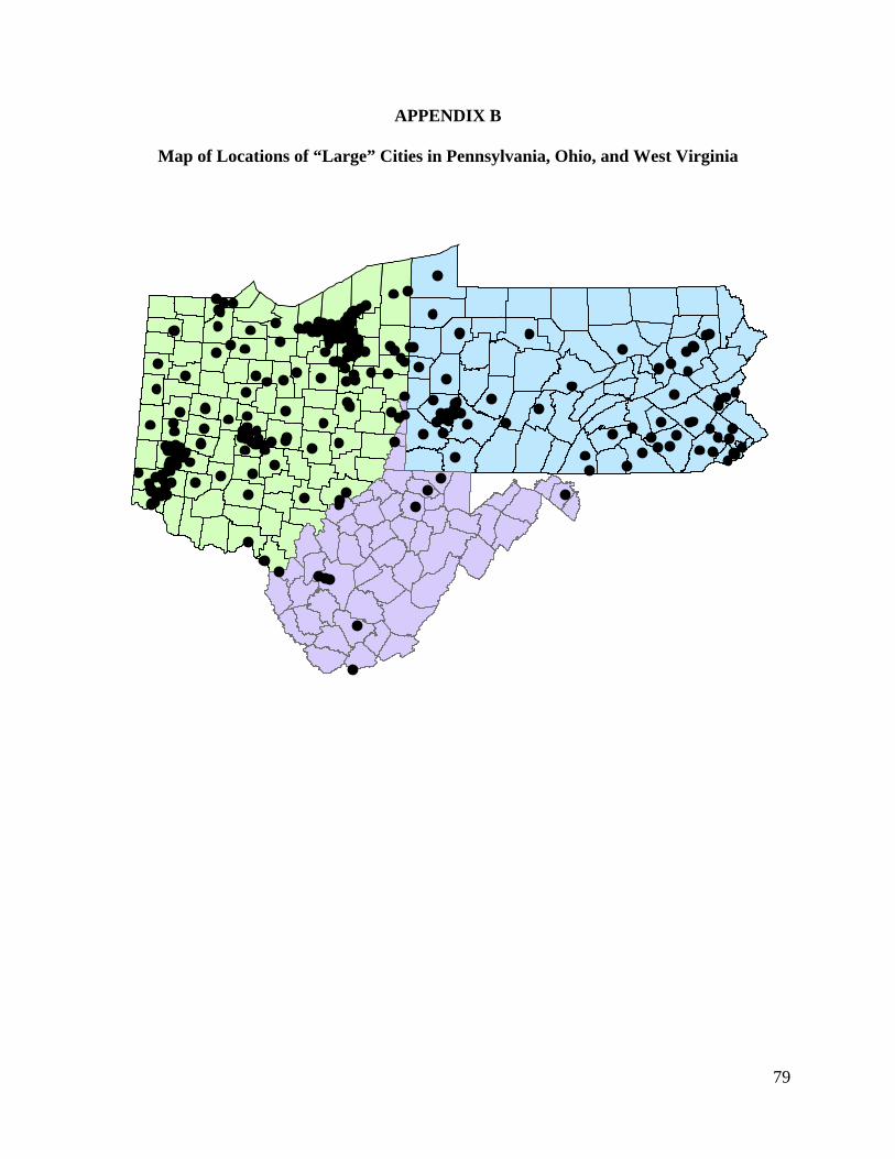
79
APPENDIX B
Map of Locations of “Large” Cities in Pennsylvania, Ohio, and West Virginia
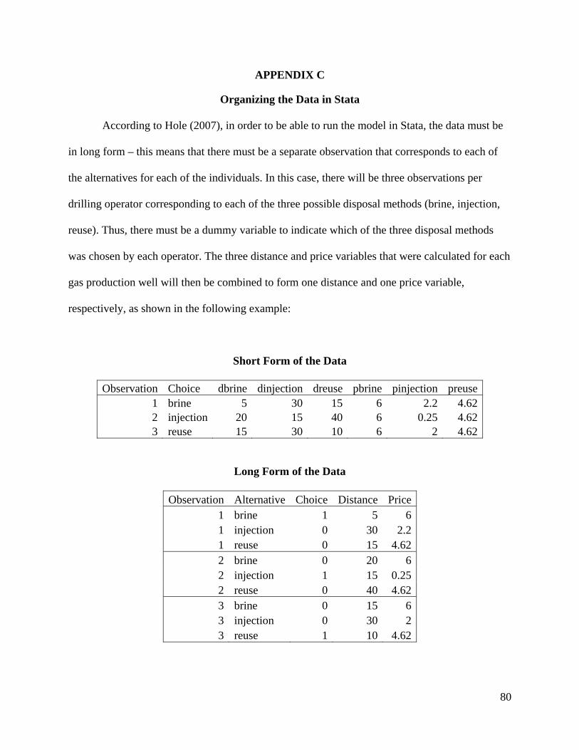
80
APPENDIX C
Organizing the Data in Stata
According to Hole (2007), in order to be able to run the model in Stata, the data must be
in long form – this means that there must be a separate observation that corresponds to each of
the alternatives for each of the individuals. In this case, there will be three observations per
drilling operator corresponding to each of the three possible disposal methods (brine, injection,
reuse). Thus, there must be a dummy variable to indicate which of the three disposal methods
was chosen by each operator. The three distance and price variables that were calculated for each
gas production well will then be combined to form one distance and one price variable,
respectively, as shown in the following example:
Short Form of the Data
Observation Choice dbrine dinjection dreuse pbrine pinjection preuse1 brine 5 30 15 6 2.2 4.622 injection 20 15 40 6 0.25 4.623 reuse 15 30 10 6 2 4.62
Long Form of the Data
Observation Alternative Choice Distance Price 1 brine 1 5 6 1 injection 0 30 2.2 1 reuse 0 15 4.62 2 brine 0 20 6 2 injection 1 15 0.25 2 reuse 0 40 4.62 3 brine 0 15 6 3 injection 0 30 2 3 reuse 1 10 4.62
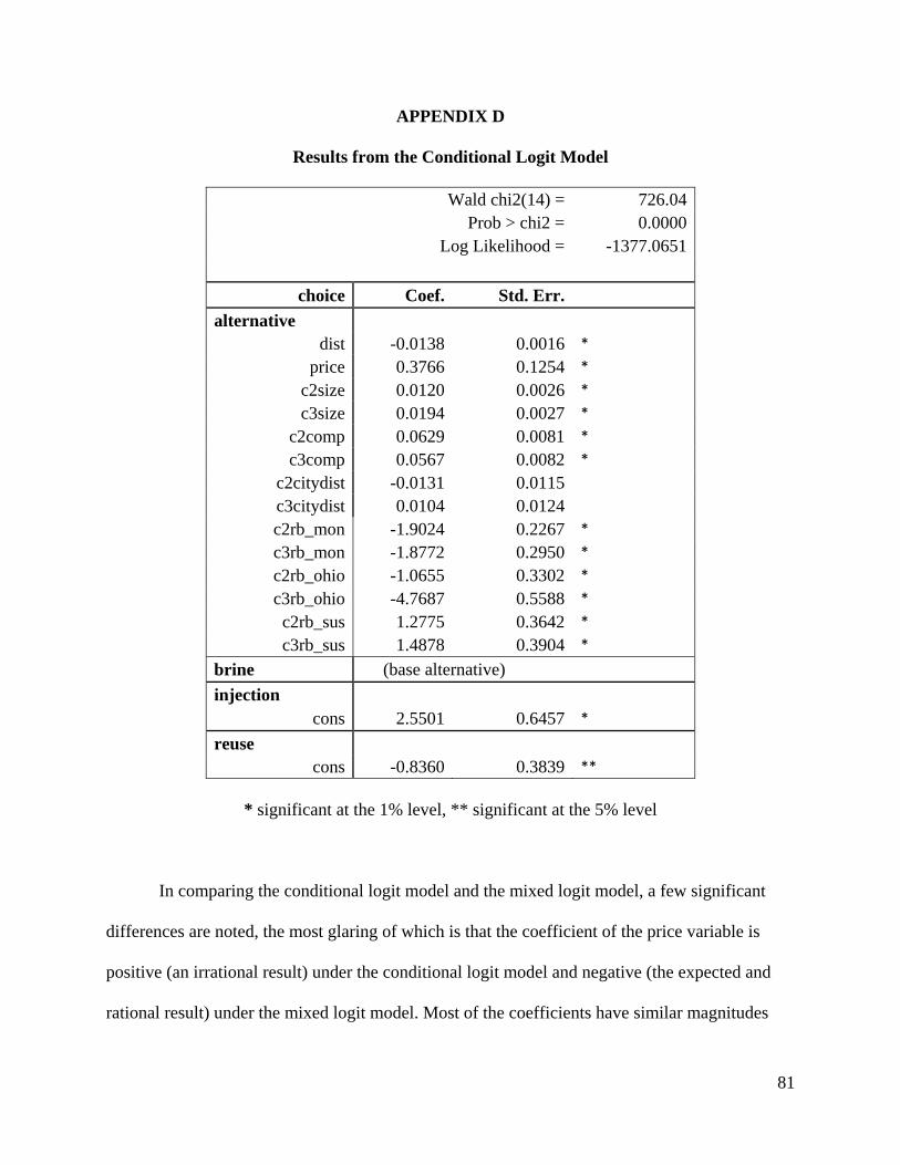
81
APPENDIX D
Results from the Conditional Logit Model
Wald chi2(14) = 726.04 Prob > chi2 = 0.0000
Log Likelihood = -1377.0651
choice Coef. Std. Err.
alternative
dist -0.0138 0.0016 *
price 0.3766 0.1254 *
c2size 0.0120 0.0026 *
c3size 0.0194 0.0027 *
c2comp 0.0629 0.0081 *
c3comp 0.0567 0.0082 *
c2citydist -0.0131 0.0115
c3citydist 0.0104 0.0124
c2rb_mon -1.9024 0.2267 *
c3rb_mon -1.8772 0.2950 *
c2rb_ohio -1.0655 0.3302 *
c3rb_ohio -4.7687 0.5588 *
c2rb_sus 1.2775 0.3642 *
c3rb_sus 1.4878 0.3904 *
brine (base alternative)
injection
cons 2.5501 0.6457 *
reuse
cons -0.8360 0.3839 **
* significant at the 1% level, ** significant at the 5% level
In comparing the conditional logit model and the mixed logit model, a few significant
differences are noted, the most glaring of which is that the coefficient of the price variable is
positive (an irrational result) under the conditional logit model and negative (the expected and
rational result) under the mixed logit model. Most of the coefficients have similar magnitudes
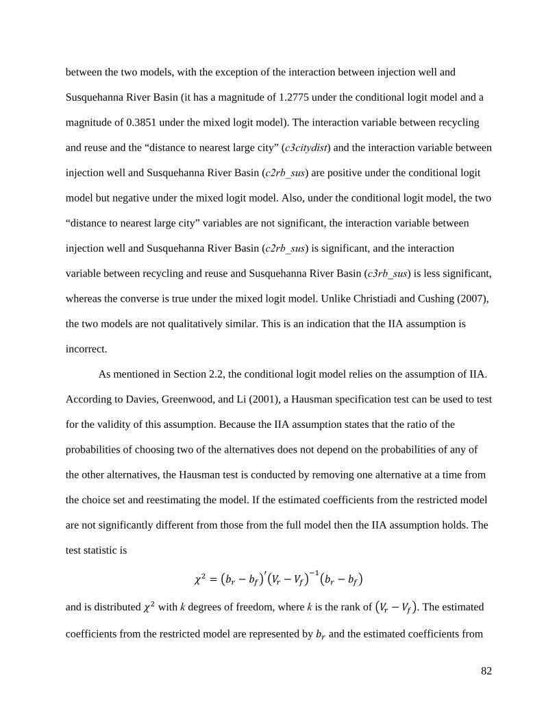
82
between the two models, with the exception of the interaction between injection well and
Susquehanna River Basin (it has a magnitude of 1.2775 under the conditional logit model and a
magnitude of 0.3851 under the mixed logit model). The interaction variable between recycling
and reuse and the “distance to nearest large city” (c3citydist) and the interaction variable between
injection well and Susquehanna River Basin (c2rb_sus) are positive under the conditional logit
model but negative under the mixed logit model. Also, under the conditional logit model, the two
“distance to nearest large city” variables are not significant, the interaction variable between
injection well and Susquehanna River Basin (c2rb_sus) is significant, and the interaction
variable between recycling and reuse and Susquehanna River Basin (c3rb_sus) is less significant,
whereas the converse is true under the mixed logit model. Unlike Christiadi and Cushing (2007),
the two models are not qualitatively similar. This is an indication that the IIA assumption is
incorrect.
As mentioned in Section 2.2, the conditional logit model relies on the assumption of IIA.
According to Davies, Greenwood, and Li (2001), a Hausman specification test can be used to test
for the validity of this assumption. Because the IIA assumption states that the ratio of the
probabilities of choosing two of the alternatives does not depend on the probabilities of any of
the other alternatives, the Hausman test is conducted by removing one alternative at a time from
the choice set and reestimating the model. If the estimated coefficients from the restricted model
are not significantly different from those from the full model then the IIA assumption holds. The
test statistic is
and is distributed with k degrees of freedom, where k is the rank of . The estimated
coefficients from the restricted model are represented by and the estimated coefficients from
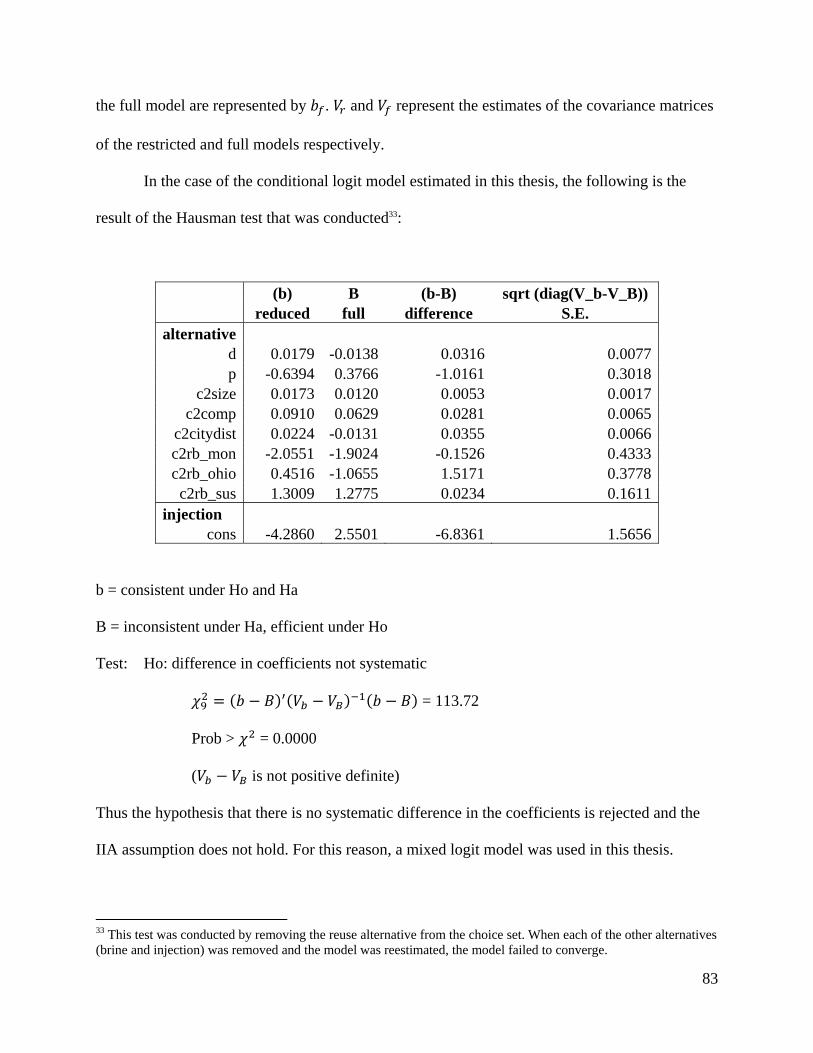
83
the full model are represented by . and represent the estimates of the covariance matrices
of the restricted and full models respectively.
In the case of the conditional logit model estimated in this thesis, the following is the
result of the Hausman test that was conducted33:
(b) B (b-B) sqrt (diag(V_b-V_B)) reduced full difference S.E. alternative
d 0.0179 -0.0138 0.0316 0.0077 p -0.6394 0.3766 -1.0161 0.3018
c2size 0.0173 0.0120 0.0053 0.0017 c2comp 0.0910 0.0629 0.0281 0.0065
c2citydist 0.0224 -0.0131 0.0355 0.0066 c2rb_mon -2.0551 -1.9024 -0.1526 0.4333 c2rb_ohio 0.4516 -1.0655 1.5171 0.3778 c2rb_sus 1.3009 1.2775 0.0234 0.1611
injection cons -4.2860 2.5501 -6.8361 1.5656
b = consistent under Ho and Ha
B = inconsistent under Ha, efficient under Ho
Test: Ho: difference in coefficients not systematic
= 113.72
Prob > = 0.0000
( is not positive definite)
Thus the hypothesis that there is no systematic difference in the coefficients is rejected and the
IIA assumption does not hold. For this reason, a mixed logit model was used in this thesis.
33 This test was conducted by removing the reuse alternative from the choice set. When each of the other alternatives (brine and injection) was removed and the model was reestimated, the model failed to converge.
84
References
Abdalla, Charles, Joy Drohan, Kristen Saacke Blunk, and Jessie Edson. Marcellus Shale Wastewater Issues in Pennsylvania – Current and Emerging Treatment and Disposal Technologies. Publication. Apr. 2011. Print.
Act 13 (Impact Fee). Pennsylvania Public Utility Commission, 2012. Web. 23 Jul. 2012. “Annual Estimates of the Resident Population for Incorporated Places: April 1, 2012 to July 1,
2011.” Census.gov. U.S. Census Bureau, 27 Jun. 2012. Web. 14 July 2012. Batte, Marvin T., Jeremy Beaverson, Neal H. Hooker, and Tim Haab. “Customer Willingness to
Pay for Multi-Ingredient, Processed Organic Food Products.” American Agricultural Economics Association Annual Meeting. Denver, CO. 1-4 Jul. 2004.
Bayoh, Isaac, Elena G. Irwin, and Timothy Haab. “Determinants of Residential Location Choice:
How Important Are Local Public Goods in Attracting Homeowners to Central City Locations?” Journal of Regional Science 46.1 (2006): 97-120.
Choi, Busik, and Jun Ishii. Consumer Perception of Warranty as Signal of Quality: An Empirical
Study of Powertrain Warranties. Working paper. Department of Economics, Amherst College, Mar. 2010. Web. 12 July 2012.
Christiadi, and Brian Cushing. “Conditional Logit, IIA, and Alternatives for Estimating Models
of Interstate Migration.” 46th Annual Meeting of the Southern Regional Science Association. Charleston, SC. 29-31 Mar. 2007.
Commonwealth of Pennsylvania. Pennsylvania Department of Environmental Protection. DEP
Calls on Natural Gas Drillers to Stop Giving Treatment Facilities Wastewater. 19 Apr. 2011. Web. 15 Apr. 2012.
Considine, Timothy J. The Economic Impacts of the Marcellus Shale: Implications for New York,
Pennsylvania, and West Virginia. Report. The American Petroleum Institute, 14 Jul. 2010. Web. 16 Jan. 2012.
Davies, Paul S., Michael J. Greenwood, and Haizheng Li. “A Conditional Logit Approach to U.S. State-to-State Migration.” Journal of Regional Science 41.2 (2001): 337-360.
Engelder, Terry, and Gary G. Lash. “Marcellus Shale Play’s Vast Resource Potential Creating Stir in Appalachia.” The American Oil & Gas Reporter. National Publishers Group Inc., May 2008. Web. 15 Apr. 2012.
GE Power and Water. Water Treatment Issues Involved in Unconventional Gas Production. Publication. Feb. 2012. Web. 14 Jun. 2012.
85
Greene, William H. “Models for Discrete Choice.” Econometric Analysis. 6th ed. Upper Saddle River, NJ: Prentice Hall, 2008. 842-847. Print.
Hakim, Danny. “Cuomo Proposal Would Restrict Gas Drilling to a Struggling Area.” The New York Times. 13 Jun. 2012. Web. 18 June 2012.
Hefley, William E. et al. The Economic Impact of the Value Chain of a Marcellus Shale Well. Working Paper. Pitt Business Working Papers – 2011, 30 Aug. 2011. Web. 13. Jun. 2012.
Hole, Arne Risa. “Fitting Mixed Logit Models using Maximum Simulated Likelihood.” The Stata Journal 7.3 (2007): 388-401.
Hynes, Stephen, and Nick Hanley. Analysing Preference Heterogeneity Using Random Parameter Logit and Latent Class Modelling Techniques. Working Paper No. 91. Department of Economics, National University of Ireland, Galway, May 2005. Web. 12 July 2012.
Kasey, Pam. “Pa. Marcellus Wastewater Industry Restructuring, Painfully.” The State Journal. 3
Jan. 2012. Web. 13 Jun. 2012. “Kasich Enacts Well Rules.” The Intelligencer/Wheeling News-Register. 11 July 2012. Web. 13
July 2012. Kelso, Matt. “Drilled Wells by Operator Over Time in PA’s Marcellus.” FracTracker.
FrackTracker, 4 May 2012. Web. 19 May 2012. Kenworthy, Tom. “Oil and Gas Link to Texas Earthquakes Studied.” ThinkProgress. Center for
American Progress Action Fund, 21 May 2012. Web. 19 Jun. 2012. Levinson, Arik. “Environmental Regulations and Manufacturers’ Location Choices: Evidence
From the Census of Manufactures.” Journal of Public Economics 62.1-2 (1996): 5-29. “Marcellus Shale – Appalachian Basin Natural Gas Play.” Geology.com. Geology.com, 2012.
Web. 15 Apr. 2012. McCurdy, Rick. “Underground Injection Wells For Produced Water Disposal.” Presentation.
U.S. Environmental Protection Agency. Web. 13 Jun. 2012. McFadden, Daniel. “Conditional Logit Analysis of Qualitative Choice Behavior.” Frontiers in
Econometrics. Ed. P. Zarembka. New York: Academic Press, 1974. 105-142.
Mittal, Devesh. “Marcellus Shale Waste Water Management Technology and Approaches.” Environmental & Natural Resources Impacts of Marcellus Shale In-Service. Penn State Extension. University Park, PA. 3 Oct. 2011.
86
Ohio Department of Natural Resources. Preliminary Report on the Northstar 1 Class II Injection Well and the Seismic Events in the Youngstown, Ohio, Area. Publication. March 2012. Web. 19 Jun. 2012.
Oil & Gas Act – Well Reporting Requirements of 2010. P.L. 169, No. 15. 22 Mar. 2010. Web. 5 May 2012.
O’Keefe, Suzanne. “Locational Choice of AFDC Recipients Within California: A Conditional Logit Analysis.” Journal of Public Economics 88.7-8 (2004): 1521-1542.
“Our Look at the Clairton Municipal Authority.” Marcellus-Shale.us. Marcellus-Shale.us, 2012. Web. 24 May 2012.
PA DEP Oil & Gas Reporting Website. Pennsylvania Department of Environmental Protection, 2012. Web. 23 May 2012.
Pennsylvania Department of Environmental Protection. PA DEP Issues Revised General Permit for Gas Wastewater Processing Facilities. PR Newswire. United Business Media, 21 Mar. 2012. Web. 25 May 2012.
Platt, Steve. “Steve Platt, EPA Region 3.” Telephone interview. 19 Mar. 2012.
Shappell, Quay. “Quay Shappell, TerrAqua Resource Management.” Telephone interview. 12 Jun. 2012.
Soraghan, Mike. “Earthquakes: Drilling Waste Wells Exempt from Earthquake Testing Rules.” EnergyWire. E&E Publishing, LLC., 22 Mar. 2012. Web. 19 Jun. 2012.
Sumi, Lisa. Shale Gas: Focus on the Marcellus Shale. Publication. Oil & Gas Accountability Project/Earthworks, May 2008. Web. 15 Apr. 2012.
Tersine, Christopher. “Christopher Tersine, PA DEP.” Personal correspondence. 20 Apr. 2012.
Tomastik, Tom. “Tom Tomastik, ODNR.” Personal interview. 21 Mar. 2012.
Train, Kenneth. “Mixed Logit.” Discrete Choice Methods With Simulation. 2nd ed. New York: Cambridge University Press, 2009. 134-150. Print.
Train, Kenneth. “Recreation Demand Models with Taste Differences Over People.” Land Economics 74.2 (1998): 230-239.
“Underground Injection Control Program.” EPA. U.S. Environmental Protection Agency, 15 Mar. 2012. Web. 15 Apr. 2012.
United States. U.S. Dept. of Energy. National Energy Technology Laboratory. Modern Shale Gas Development in the United States: A Primer. Apr. 2009. Web. 15 Apr. 2012
87
United States. U.S. Dept. of the Interior, U.S. Geological Survey. Assessment of Undiscovered
Oil and Gas Resources of the Appalachian Basin Province, 2002. Feb. 2003. Web. 15 Apr. 2012.
United States. U.S. Energy Information Administration. Annual Energy Outlook 2011 With
Projections to 2035. Apr. 2011. Web. 15 Apr. 2012. United States. U.S. Energy Information Administration. Annual Energy Outlook 2012 With
Projections to 2035. Jun. 2012. Web. 1 Jun. 2012. United States. U.S. Geological Survey. Assessment of Undiscovered Oil and Gas Resources of
the Devonian Marcellus Shale of the Appalachian Basin Province, 2011. By James L. Coleman et al. Aug. 2011. Web. 15 Apr. 2012.
U.S. Environmental Protection Agency, Region 3. Consent Agreement and Final Order: EXCO
Resources (PA), LLC. 30 Mar. 2012. Web. 25 May 2012. U.S. Environmental Protection Agency, Region 3. Jenner Township, PA: Notice of Proposal to
Issue a Draft Final Permit and Opportunity for Public Comment. 2011. Web. 15 May 2012.
U.S. Environmental Protection Agency, Region 3. Range Resources, Waterford, PA: Notice of
Proposal to Issue a Draft Final Permit and Opportunity for Public Comment. 2011. Web. 15 May 2012.
Yoxtheimer, David. “David Yoxtheimer, The Penn State Marcellus Center for Outreach and
Research.” Personal Interview. 23 May 2012. Yoxtheimer, David. “How Much Natural Gas Can the Marcellus Shale Produce?” Penn State
Extension. Penn State College of Agricultural Sciences, 5 Feb. 2012. Web. 15 Apr. 2012.