MapReduce Algorithm DesignData-Intensive Information Processing Applications ― Session #3

Jimmy LinUniversity of Maryland

Tuesday, February 9, 2010

This work is licensed under a Creative Commons Attribution-Noncommercial-Share Alike 3.0 United StatesSee http://creativecommons.org/licenses/by-nc-sa/3.0/us/ for details

Source: Wikipedia (Japanese rock garden)

Today’s Agenda “The datacenter is the computer”

Understanding the design of warehouse-sized computes

MapReduce algorithm design How do you express everything in terms of m, r, c, p? Toward “design patterns”

The datacenter is the computer

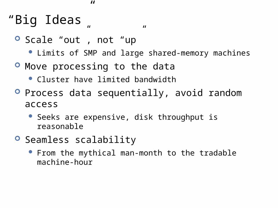
“Big Ideas” Scale “out”, not “up”

Limits of SMP and large shared-memory machines

Move processing to the data Cluster have limited bandwidth

Process data sequentially, avoid random access Seeks are expensive, disk throughput is reasonable

Seamless scalability From the mythical man-month to the tradable machine-hour

Source: Wikipedia (The Dalles, Oregon)

Source: NY Times (6/14/2006)

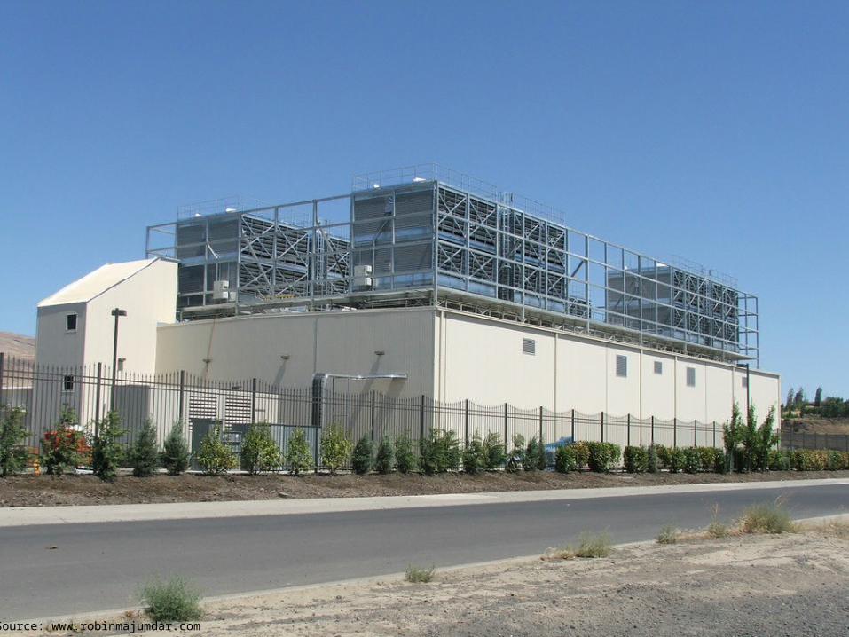
Source: www.robinmajumdar.com

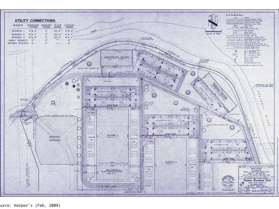
Source: Harper’s (Feb, 2008)

Source: Bonneville Power Administration

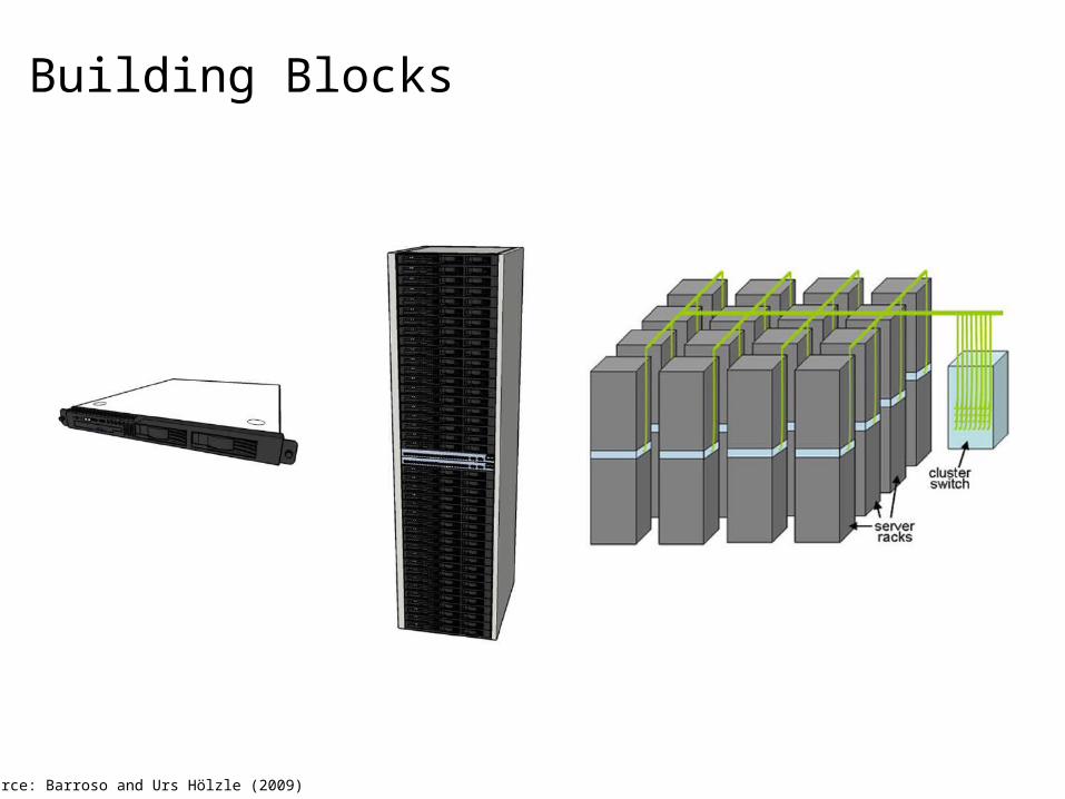
Building Blocks

Source: Barroso and Urs Hölzle (2009)

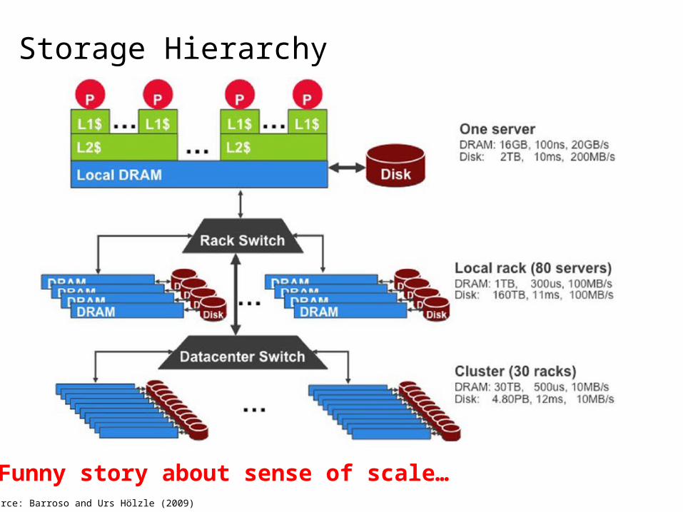
Storage Hierarchy

Funny story about sense of scale…Source: Barroso and Urs Hölzle (2009)

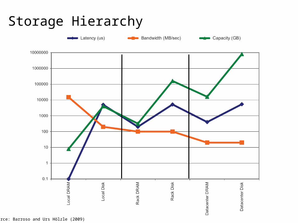
Storage Hierarchy

Source: Barroso and Urs Hölzle (2009)

Anatomy of a Datacenter

Source: Barroso and Urs Hölzle (2009)

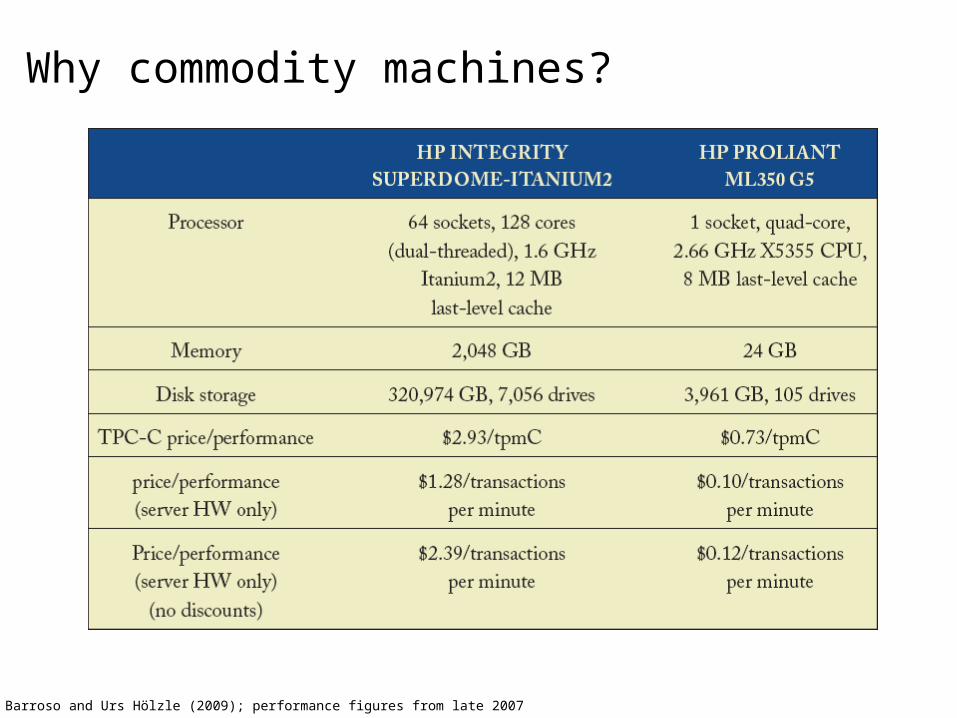
Why commodity machines?

Source: Barroso and Urs Hölzle (2009); performance figures from late 2007

What about communication? Nodes need to talk to each other!

SMP: latencies ~100 ns LAN: latencies ~100 s

Scaling “up” vs. scaling “out” Smaller cluster of SMP machines vs. larger cluster of commodity

machines E.g., 8 128-core machines vs. 128 8-core machines Note: no single SMP machine is big enough

Let’s model communication overhead…

Source: analysis on this an subsequent slides from Barroso and Urs Hölzle (2009)

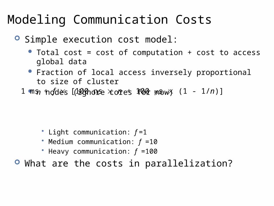
Modeling Communication Costs Simple execution cost model:

Total cost = cost of computation + cost to access global data Fraction of local access inversely proportional to size of cluster n nodes (ignore cores for now)

• Light communication: f =1• Medium communication: f =10• Heavy communication: f =100

What are the costs in parallelization?

1 ms + f [100 ns n + 100 s (1 - 1/n)]

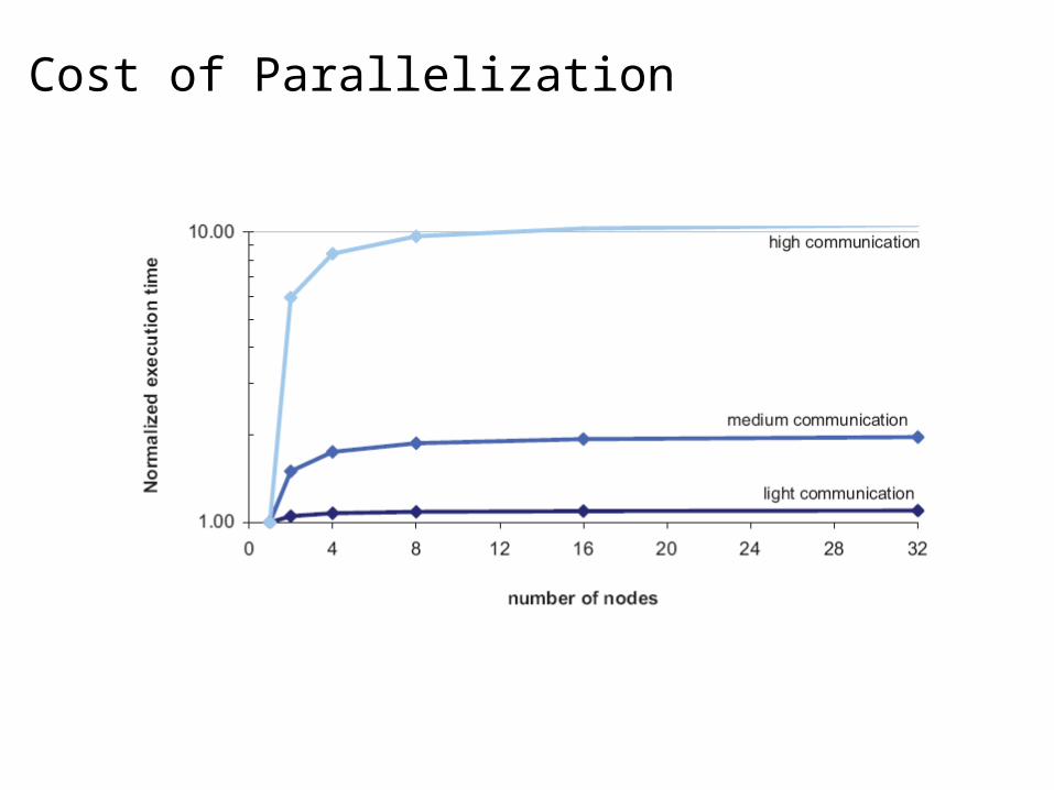
Cost of Parallelization

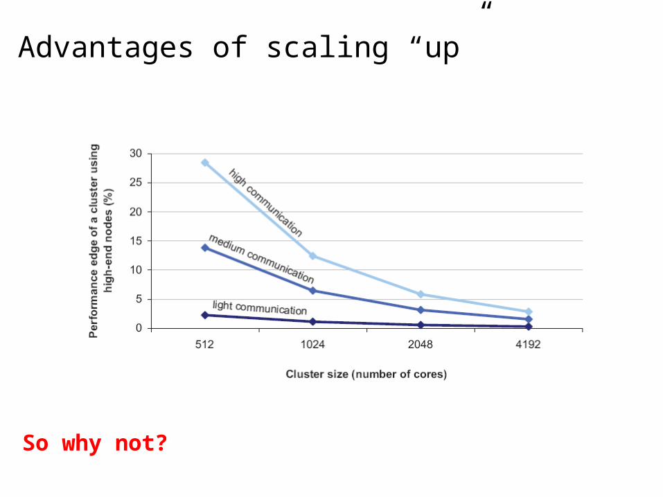
Advantages of scaling “up”

So why not?

Seeks vs. Scans Consider a 1 TB database with 100 byte records

We want to update 1 percent of the records

Scenario 1: random access Each update takes ~30 ms (seek, read, write) 108 updates = ~35 days

Scenario 2: rewrite all records Assume 100 MB/s throughput Time = 5.6 hours(!)

Lesson: avoid random seeks!

Source: Ted Dunning, on Hadoop mailing list

Justifying the “Big Ideas” Scale “out”, not “up”

Limits of SMP and large shared-memory machines

Move processing to the data Cluster have limited bandwidth

Process data sequentially, avoid random access Seeks are expensive, disk throughput is reasonable

Seamless scalability From the mythical man-month to the tradable machine-hour

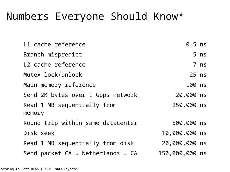
Numbers Everyone Should Know*

L1 cache reference 0.5 ns

Branch mispredict 5 ns

L2 cache reference 7 ns

Mutex lock/unlock 25 ns

Main memory reference 100 ns

Send 2K bytes over 1 Gbps network 20,000 ns

Read 1 MB sequentially from memory 250,000 ns

Round trip within same datacenter 500,000 ns

Disk seek 10,000,000 ns

Read 1 MB sequentially from disk 20,000,000 ns

Send packet CA → Netherlands → CA 150,000,000 ns

* According to Jeff Dean (LADIS 2009 keynote)

MapReduce Algorithm Design

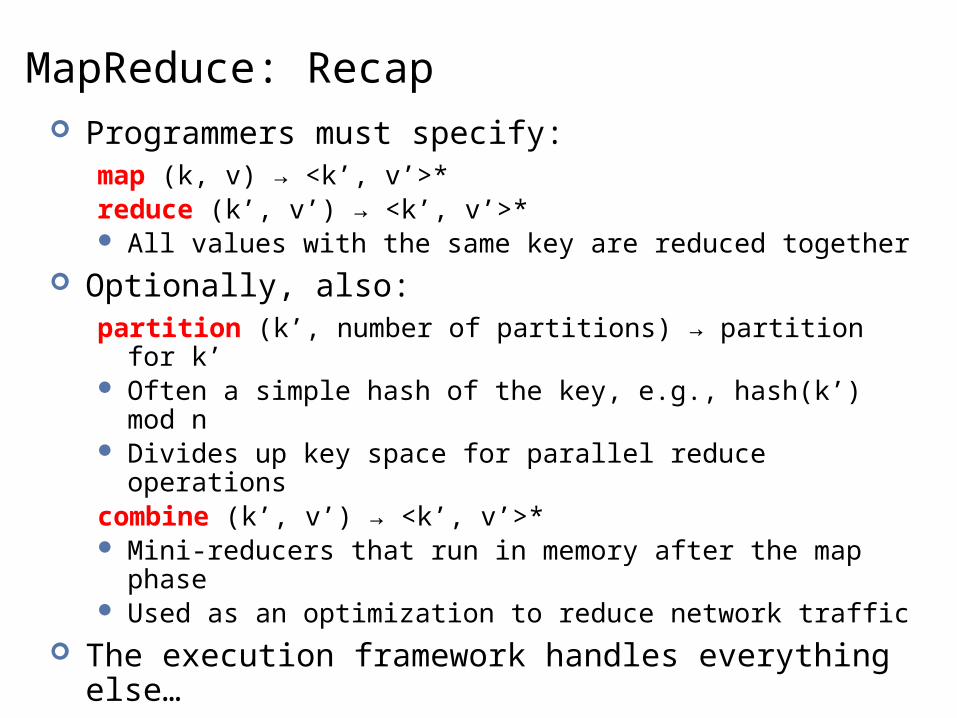
MapReduce: Recap Programmers must specify:

map (k, v) → <k’, v’>*reduce (k’, v’) → <k’, v’>* All values with the same key are reduced together

Optionally, also:partition (k’, number of partitions) → partition for k’ Often a simple hash of the key, e.g., hash(k’) mod n Divides up key space for parallel reduce operationscombine (k’, v’) → <k’, v’>* Mini-reducers that run in memory after the map phase Used as an optimization to reduce network traffic

The execution framework handles everything else…

combinecombine combine combine

ba 1 2 c 9 a c5 2 b c7 8

partition partition partition partition

mapmap map map

k1 k2 k3 k4 k5 k6v1 v2 v3 v4 v5 v6

ba 1 2 c c3 6 a c5 2 b c7 8

Shuffle and Sort: aggregate values by keys

reduce reduce reduce

a 1 5 b 2 7 c 2 9 8

r1 s1 r2 s2 r3 s3

“Everything Else” The execution framework handles everything else…

Scheduling: assigns workers to map and reduce tasks “Data distribution”: moves processes to data Synchronization: gathers, sorts, and shuffles intermediate data Errors and faults: detects worker failures and restarts

Limited control over data and execution flow All algorithms must expressed in m, r, c, p

You don’t know: Where mappers and reducers run When a mapper or reducer begins or finishes Which input a particular mapper is processing Which intermediate key a particular reducer is processing

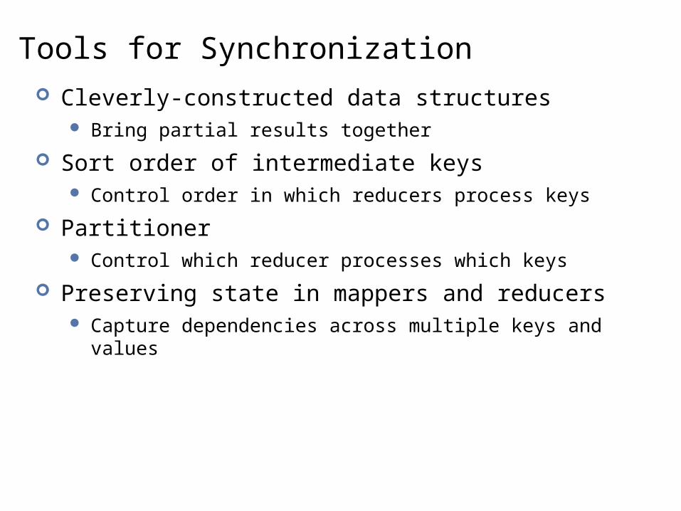
Tools for Synchronization Cleverly-constructed data structures

Bring partial results together

Sort order of intermediate keys Control order in which reducers process keys

Partitioner Control which reducer processes which keys

Preserving state in mappers and reducers Capture dependencies across multiple keys and values

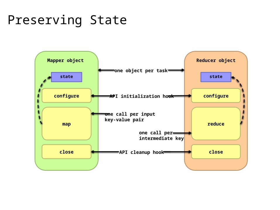
Preserving State

Mapper object

configure

map

close

stateone object per task

Reducer object

configure

reduce

close

state

one call per input key-value pair

one call per intermediate key

API initialization hook

API cleanup hook

Scalable Hadoop Algorithms: Themes Avoid object creation

Inherently costly operation Garbage collection

Avoid buffering Limited heap size Works for small datasets, but won’t scale!

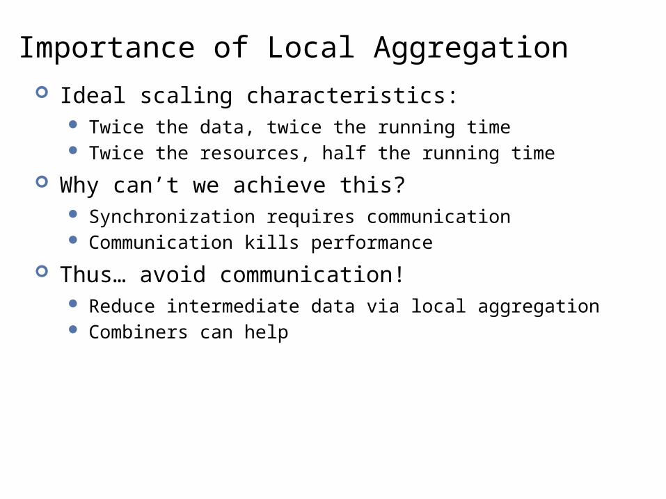
Importance of Local Aggregation Ideal scaling characteristics:

Twice the data, twice the running time Twice the resources, half the running time

Why can’t we achieve this? Synchronization requires communication Communication kills performance

Thus… avoid communication! Reduce intermediate data via local aggregation Combiners can help

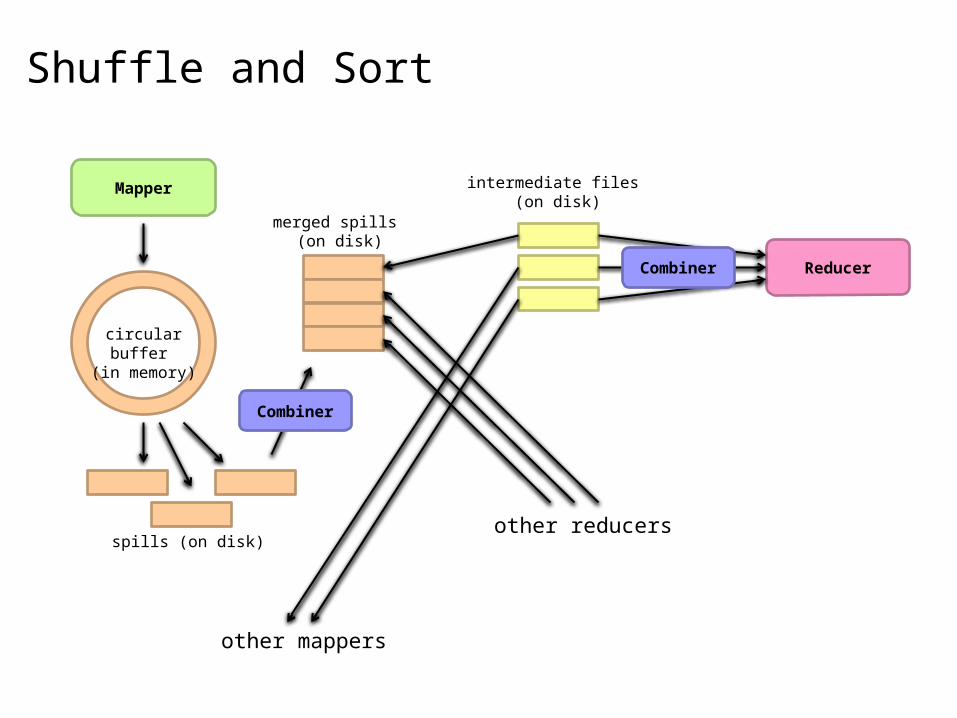
Shuffle and Sort

Mapper

Reducer

other mappers

other reducers

circular buffer (in memory)

spills (on disk)

merged spills (on disk)

intermediate files (on disk)

Combiner

Combiner

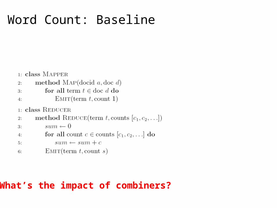
Word Count: Baseline

What’s the impact of combiners?

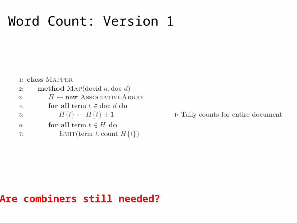
Word Count: Version 1

Are combiners still needed?

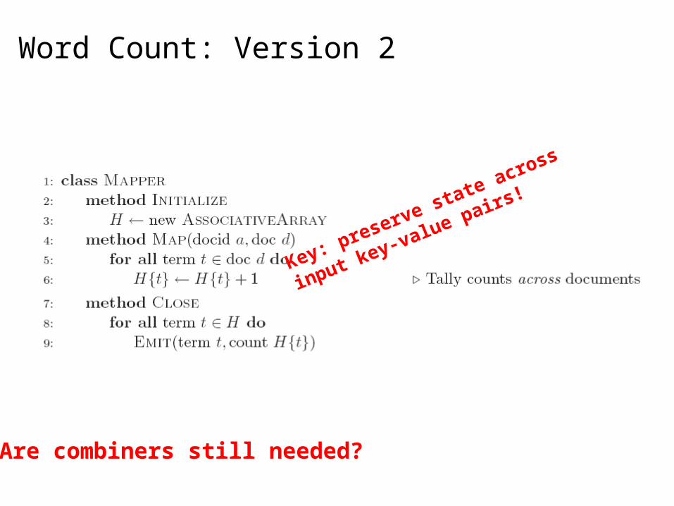
Word Count: Version 2

Are combiners still needed?

Key: preserve state across

input key-value pairs!

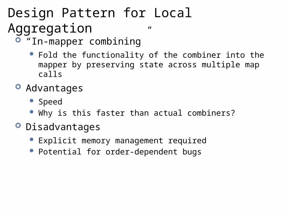
Design Pattern for Local Aggregation “In-mapper combining”

Fold the functionality of the combiner into the mapper by preserving state across multiple map calls

Advantages Speed Why is this faster than actual combiners?

Disadvantages Explicit memory management required Potential for order-dependent bugs

Combiner Design Combiners and reducers share same method signature

Sometimes, reducers can serve as combiners Often, not…

Remember: combiner are optional optimizations Should not affect algorithm correctness May be run 0, 1, or multiple times

Example: find average of all integers associated with the same key

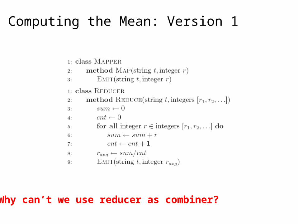
Computing the Mean: Version 1

Why can’t we use reducer as combiner?

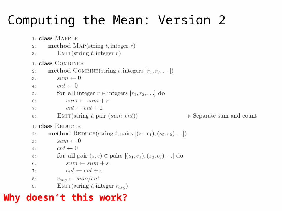
Computing the Mean: Version 2

Why doesn’t this work?

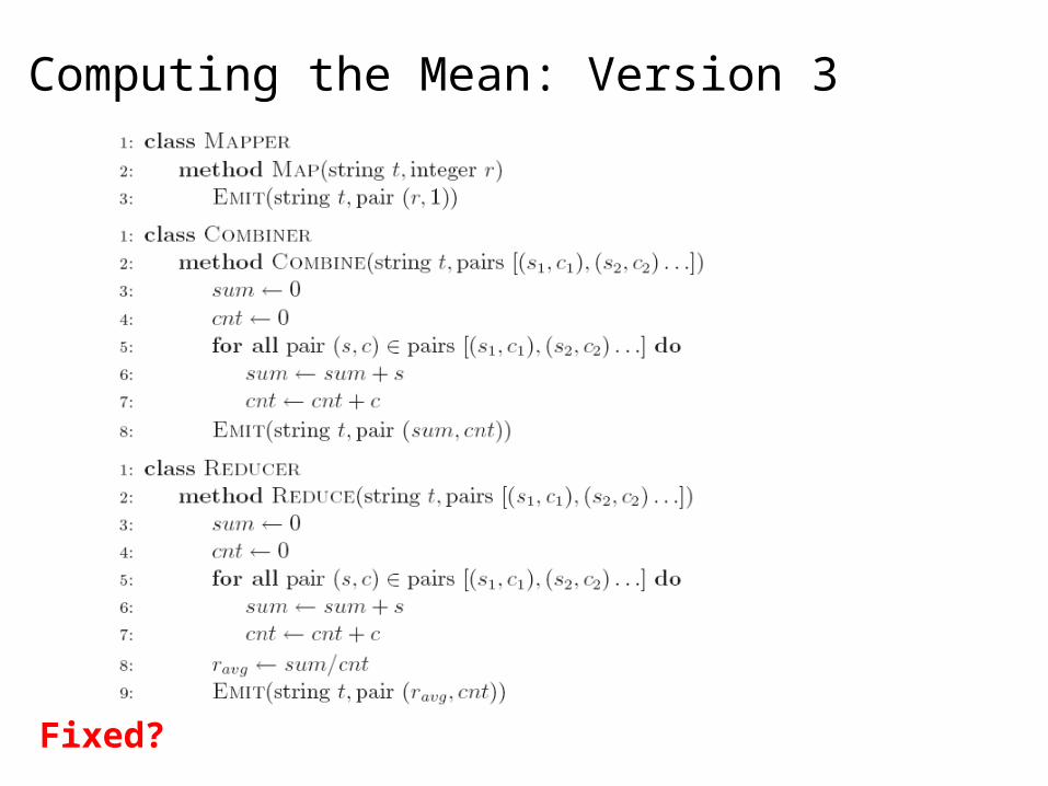
Computing the Mean: Version 3

Fixed?

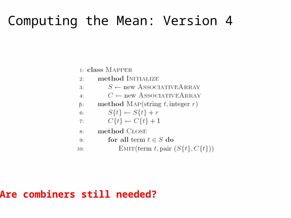
Computing the Mean: Version 4

Are combiners still needed?

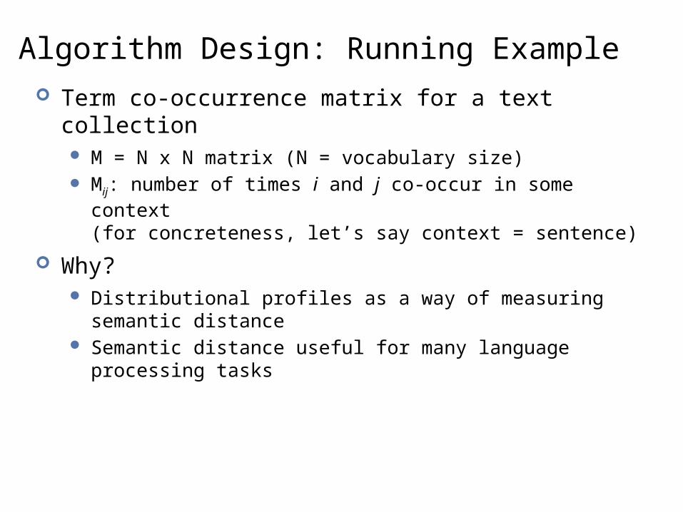
Algorithm Design: Running Example Term co-occurrence matrix for a text collection

M = N x N matrix (N = vocabulary size) Mij: number of times i and j co-occur in some context

(for concreteness, let’s say context = sentence)

Why? Distributional profiles as a way of measuring semantic distance Semantic distance useful for many language processing tasks

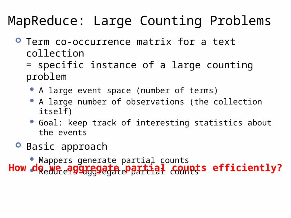
MapReduce: Large Counting Problems Term co-occurrence matrix for a text collection

= specific instance of a large counting problem A large event space (number of terms) A large number of observations (the collection itself) Goal: keep track of interesting statistics about the events

Basic approach Mappers generate partial counts Reducers aggregate partial counts

How do we aggregate partial counts efficiently?

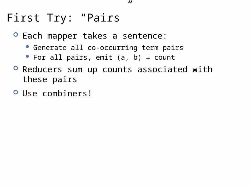
First Try: “Pairs” Each mapper takes a sentence:

Generate all co-occurring term pairs For all pairs, emit (a, b) → count

Reducers sum up counts associated with these pairs

Use combiners!

Pairs: Pseudo-Code

“Pairs” Analysis Advantages

Easy to implement, easy to understand

Disadvantages Lots of pairs to sort and shuffle around (upper bound?) Not many opportunities for combiners to work

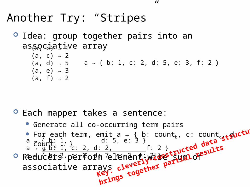
Another Try: “Stripes” Idea: group together pairs into an associative array

Each mapper takes a sentence: Generate all co-occurring term pairs For each term, emit a → { b: countb, c: countc, d: countd … }

Reducers perform element-wise sum of associative arrays

(a, b) → 1 (a, c) → 2 (a, d) → 5 (a, e) → 3 (a, f) → 2

a → { b: 1, c: 2, d: 5, e: 3, f: 2 }

a → { b: 1, d: 5, e: 3 }a → { b: 1, c: 2, d: 2, f: 2 }a → { b: 2, c: 2, d: 7, e: 3, f: 2 }

+

Key: cleverly-constructed data structure

brings together partial results

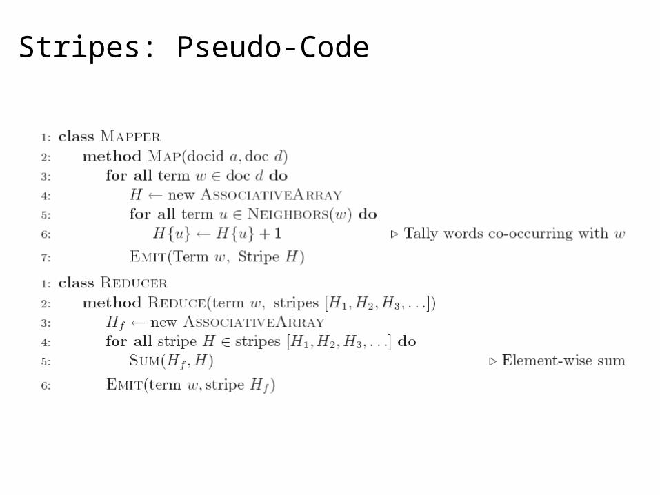
Stripes: Pseudo-Code

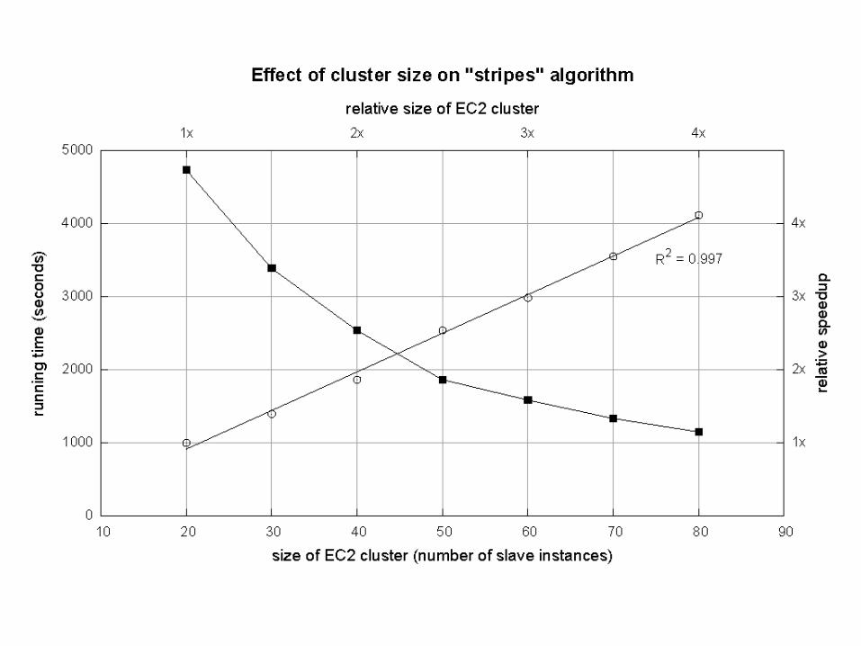
“Stripes” Analysis Advantages

Far less sorting and shuffling of key-value pairs Can make better use of combiners

Disadvantages More difficult to implement Underlying object more heavyweight Fundamental limitation in terms of size of event space

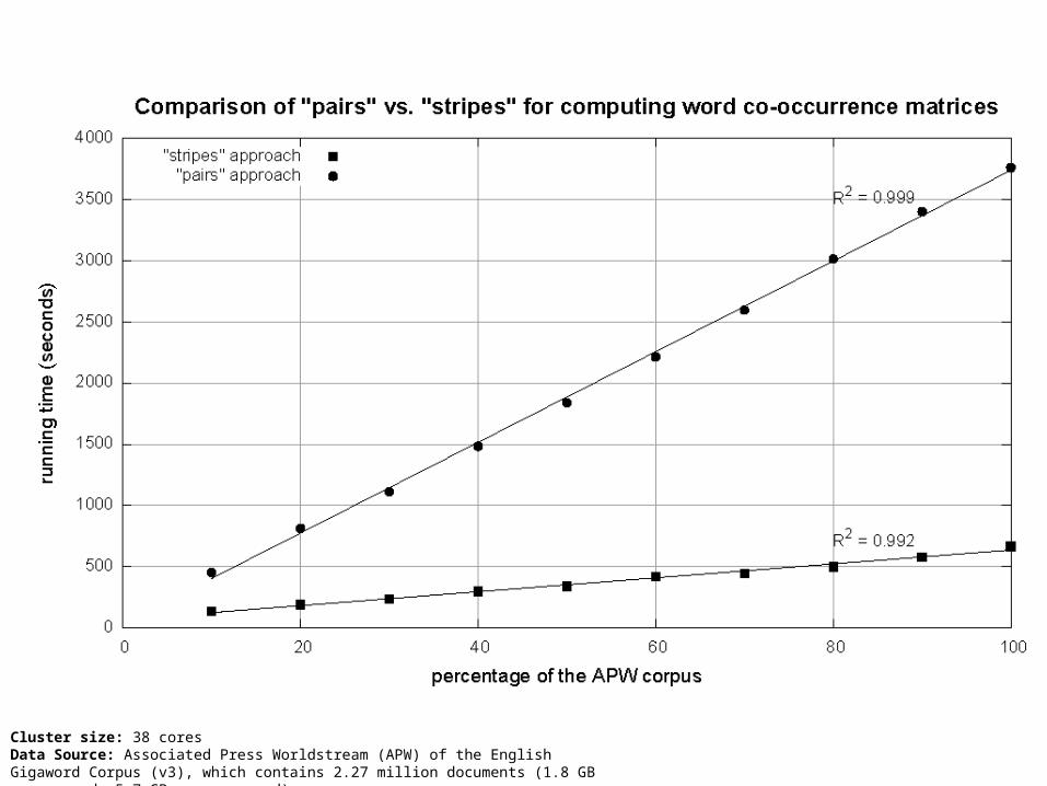
Cluster size: 38 coresData Source: Associated Press Worldstream (APW) of the English Gigaword Corpus (v3), which contains 2.27 million documents (1.8 GB compressed, 5.7 GB uncompressed)

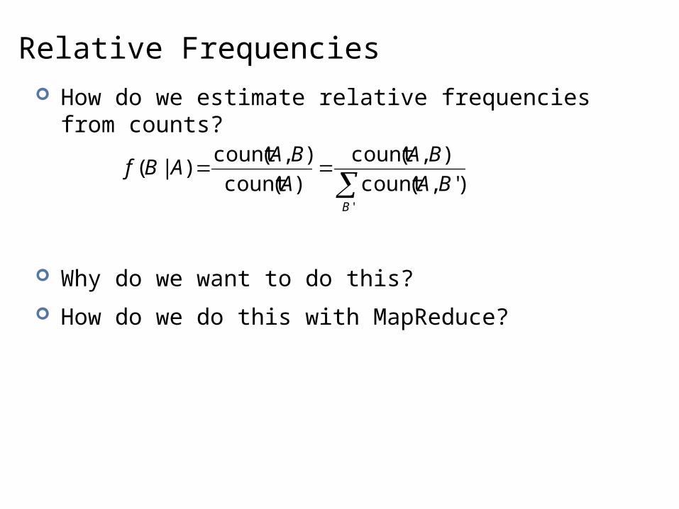
Relative Frequencies How do we estimate relative frequencies from counts?

Why do we want to do this?

How do we do this with MapReduce?

'

)',(count

),(count

)(count

),(count)|(

B

BA

BA

A

BAABf

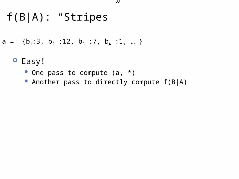
f(B|A): “Stripes”

Easy! One pass to compute (a, *) Another pass to directly compute f(B|A)

a → {b1:3, b2 :12, b3 :7, b4 :1, … }

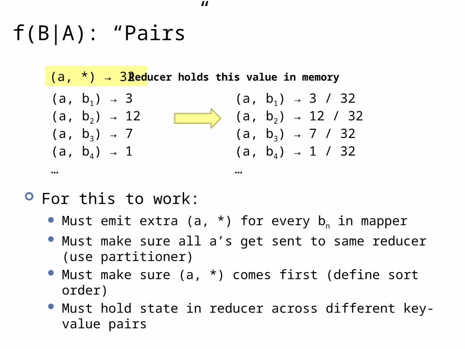
f(B|A): “Pairs”

For this to work: Must emit extra (a, *) for every bn in mapper Must make sure all a’s get sent to same reducer (use partitioner) Must make sure (a, *) comes first (define sort order) Must hold state in reducer across different key-value pairs

(a, b1) → 3 (a, b2) → 12 (a, b3) → 7(a, b4) → 1 …

(a, *) → 32

(a, b1) → 3 / 32 (a, b2) → 12 / 32(a, b3) → 7 / 32(a, b4) → 1 / 32…

Reducer holds this value in memory

“Order Inversion” Common design pattern

Computing relative frequencies requires marginal counts But marginal cannot be computed until you see all counts Buffering is a bad idea! Trick: getting the marginal counts to arrive at the reducer before

the joint counts

Optimizations Apply in-memory combining pattern to accumulate marginal counts Should we apply combiners?

Synchronization: Pairs vs. Stripes Approach 1: turn synchronization into an ordering problem

Sort keys into correct order of computation Partition key space so that each reducer gets the appropriate set

of partial results Hold state in reducer across multiple key-value pairs to perform

computation Illustrated by the “pairs” approach

Approach 2: construct data structures that bring partial results together Each reducer receives all the data it needs to complete the

computation Illustrated by the “stripes” approach

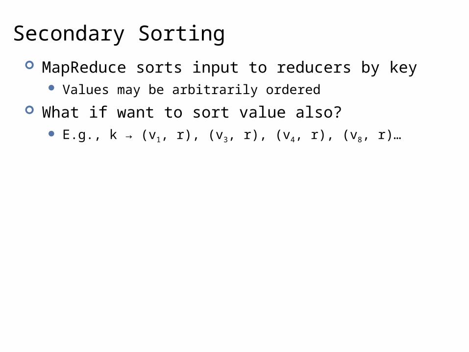
Secondary Sorting MapReduce sorts input to reducers by key

Values may be arbitrarily ordered

What if want to sort value also? E.g., k → (v1, r), (v3, r), (v4, r), (v8, r)…

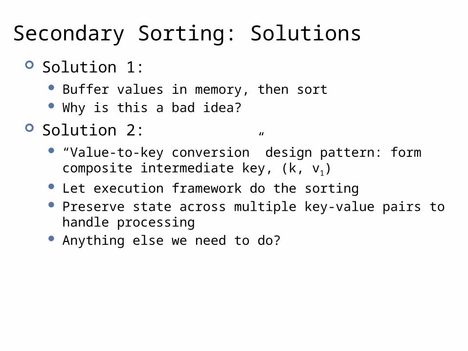
Secondary Sorting: Solutions Solution 1:

Buffer values in memory, then sort Why is this a bad idea?

Solution 2: “Value-to-key conversion” design pattern: form composite

intermediate key, (k, v1) Let execution framework do the sorting Preserve state across multiple key-value pairs to handle

processing Anything else we need to do?

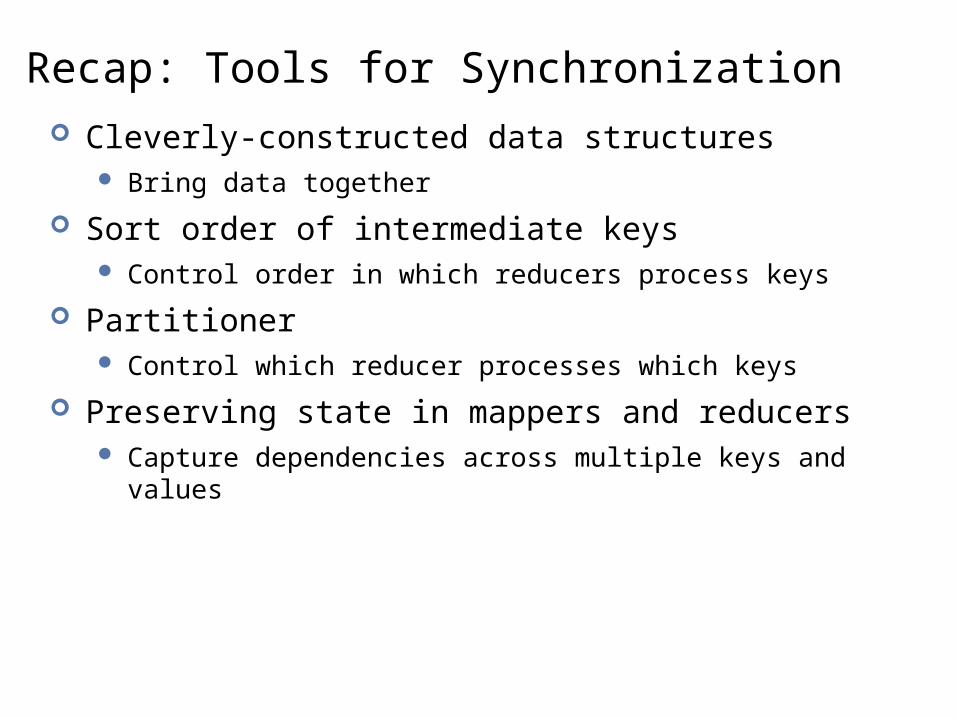
Recap: Tools for Synchronization Cleverly-constructed data structures

Bring data together

Sort order of intermediate keys Control order in which reducers process keys

Partitioner Control which reducer processes which keys

Preserving state in mappers and reducers Capture dependencies across multiple keys and values

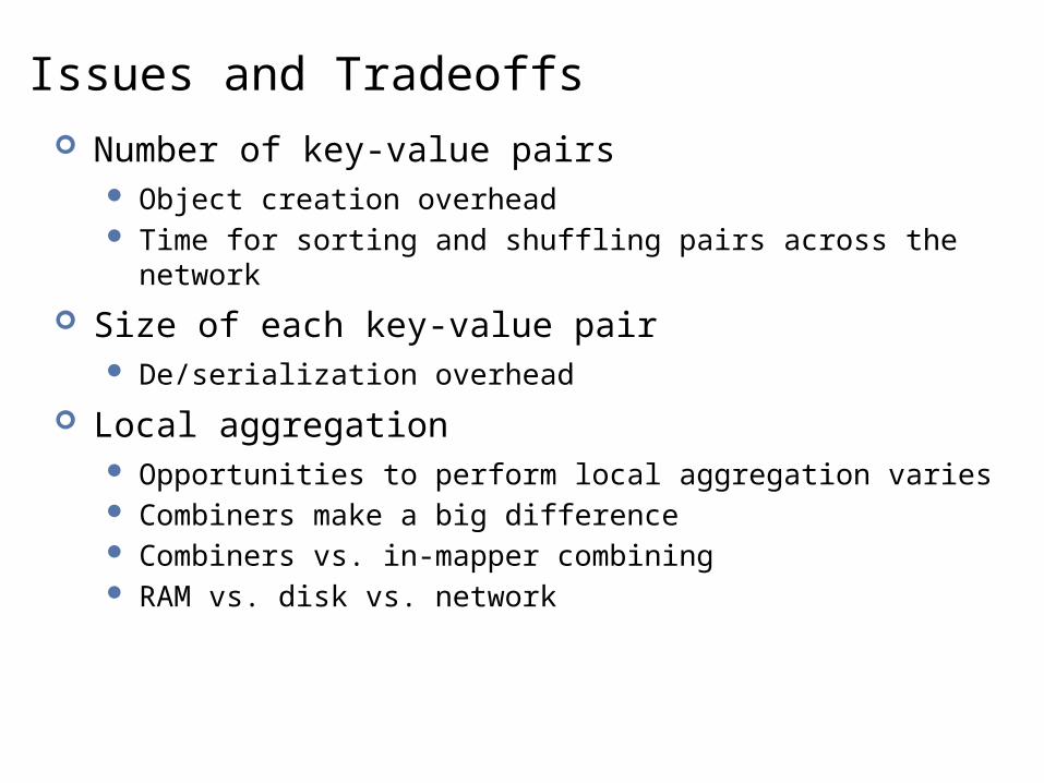
Issues and Tradeoffs Number of key-value pairs

Object creation overhead Time for sorting and shuffling pairs across the network

Size of each key-value pair De/serialization overhead

Local aggregation Opportunities to perform local aggregation varies Combiners make a big difference Combiners vs. in-mapper combining RAM vs. disk vs. network

Debugging at Scale Works on small datasets, won’t scale… why?

Memory management issues (buffering and object creation) Too much intermediate data Mangled input records

Real-world data is messy! Word count: how many unique words in Wikipedia? There’s no such thing as “consistent data” Watch out for corner cases Isolate unexpected behavior, bring local

Source: Wikipedia (Japanese rock garden)

Questions?