White Paper

Mapping with auxiliary data

Methodologies for advanced mapping and applications to

Geological Modeling

Mapping with auxiliary data Methodologies for advanced mapping and applications to Geological Modeling

Use interpolation methods that allow evaluating and enhancing the reliability of your maps.

The objective of any serious mapping is to obtain a realistic and reliable image of the studied phenomenon. This can be done by working with a lot of data samples, regularly distributed over the area of interest, each mapping algorithm being efficient in such a context. In many cases, samples are unfortunately rare and irregularly distributed, due to geological or physical constraints which limit the possibility to get samples and/or to economic constraints. It is then of primary importance to apply mapping algorithms that are able to mix different sources of information, including fuzzy data.

This white paper shows you how the geostatistical approach based on kriging, with all its variations, is the solution for a high quality and reliable mapping even in complex cases. It details the different methods for assimilating various sources of information, taking into account the reliability of each source and how the uncertainty associated with any mapping result can be estimated and reduced.

Geovariances has been applying this geostatistical approach for more than twenty years in the various contexts, from geological modelling in Oil &Gas and Mining industries to pollution mapping or remediation projects of sites contaminated with radionuclides.

Aim of mapping algorithms

Mapping consists in determining the unknown value of a given parameter at a given location, results being represented in 2D or 3D maps, studied parameter values distribution being displayed by mean of level contours or colormaps. In the past, this operation was done by hand. Nowadays, it is made with specialized software in which many different estimation algorithms have been implemented.

The aim of this document is to provide an overview of the main geostatistical estimation algorithms that can be used in difficult conditions, when data samples are rare and irregularly distributed in space. It shows how the use of auxiliary data sources can help enhancing the results and reducing the uncertainty. A special focus is put on the pros and cons of each method and on their application conditions.

Some application examples of the most efficient algorithms and workflows are presented.

The main strength of geostatistical techniques is their ability to take into account the spatial structure of the studied phenomenon (by mean of the variogram). Another advantage is the fact that the uncertainty attached to each result is always provided. Several algorithms are available, all based on Kriging or on geostatistical simulation algorithms conditioned to data by kriging.

The most common methods are presented below. For clarity, they can be regrouped into few categories:

Kriging with a multivariate model

Cokriging

Cokriging estimates are calculated by making a linear combination of neighbour samples, combining all the measured variables. With two variables Z and T, it is given by the formula:

The cokriging estimate is designed to ensure that the mean of the estimation error is null (non-bias condition) and that the variance of the estimation error is minimal (optimality condition).

Cokriging requires a multivariate model of correlation (linear model of coregionalization). It means that the variograms of each variable and all the cross-variograms must be calculated and fitted within a consistent mathematical framework. Usually, when variables show a high correlation, all the variograms and cross-variograms may be fitted with the same components.

( ) ( ) ( )∑∑ α+λ=j

jji

ii0*cok xTxZxZ

Are you confident in the quality of your maps?

With multivariate geostatistical techniques, benefit from all available information.

Cokriging corresponds to an optimal use of correlated data. It must be noted that all the variables play the same role in this method. It can be applied only in stationary environments (no spatial trend in the data).

Collocated cokriging

Collocated cokriging is a variation of cokriging which is optimized for the case where one of the variables is known at target points. For example, it is useful when one variable is known at well locations and the other one is provided as a full map, the interpolation being made at each node of this map. It is frequently used for estimating Porosity from well data and a seismic impedance map. It is often difficult to fit a bivariate model on variograms and cross-variograms when data are sparse. When one of the variables is dense, known at each node of the target grid, it might be interesting to calculate the model from this dense dataset and make an assumption on the similar behaviour of the other variable. This method is commonly used in collocated cokriging, the assumption being called the Markov-Bayes assumption. With two variables Z and T, the bivariate model is calculated from the univariate model of the dense dataset using the following relationships:

Application

Issue: Porosity mapping with few well data

In the example, a porosity map derived from seismic data is available, but only few wells. At the field scale, the well data spatial distribution is not regular enough to guarantee the result quality.

Solution: Collocated cokriging with well data and the auxiliary source map.

Result: Consistent map taking benefit of all data sources (Fig. 1)

With multivariate geostatistical techniques, refine your maps and reduce their uncertainty.

Figure 1: Comparison between Porosity maps with well data only (left) and well data + auxiliary map (right).

Kriging with a univariate model and various data sources

Kriging with external drift

Kriging with external drift (KED) is the preferred industry solution to combine well and seismic derived data, as it is easier to implement than cokriging and can be applied in presence of regional trends (non-stationary context).

With KED, variables are not equivalent. There is a primary variable to be estimated, with the help of secondary variables. We assume that the secondary variables (e.g. seismic information) provide low frequency information about the primary variable, with the high frequencies contained in the residuals. The KED system contains a linear transformation to the seismic data and a variogram of residuals. They are combined to provide, in one step only, an estimate that matches the well data and is consistent with the non-stationary trend coming from the seismic data.

In the external drift method, this low frequency trend (Figure 2) is included in the kriging system as a drift, therefore as a universality condition, not as an additional variable contributing in the estimation (as in collocated cokriging).

Figure 2: Schema where the signal Z(x) is decomposed into a low frequency

component (the drift) and high frequency residuals (R(x))

Kriging Collocated

In a Kriging with external drift, the model is non-stationary if the drift is itself non-stationary, but its covariance part is stationary (the variogram of the residuals). Therefore, the variable is estimated with a model combining both stationary and non-stationary parts. These techniques require the computation and the fitting of a non-stationary spatial correlation model.

Kriging with Bayesian drift

Kriging with Bayesian drift can be considered as a generalization of KED. Computing a reliable trend may be difficult in the case of sparse data. Bayesian kriging (Omre 1987) allows accounting for prior knowledge in such cases. In this framework, unknown drift coefficients are considered as random variables and assumed to have a Gaussian joint distribution. Within the Bayesian framework, the distribution of these variables can be provided by the geoscientist (a Gaussian distribution defined by the mean and standard deviation of the linear regression slope coefficient and the correlations between them). As for KED, the drift functions and the covariance of the residuals have to be provided (non stationary spatial model). The covariance is a challenging part as the trend is not yet known at this stage. It has to be inferred from prior knowledge.

Applications

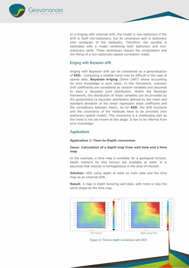
Application 1: Time-to-Depth conversion

Issue: Calculation of a depth map from well data and a time map

In the example, a time map is available for a geological horizon. Depth markers for this horizon are available at wells. It is assumed that velocity is homogeneous in the area of interest.

Solution: KED using depth at wells as main data and the time map as an external drift.

Result: A map in depth honoring well data, with more or less the same shape as the time map

Figure 3: Time-to-depth conversion with KED

0

0

1000

1000

2000

2000

3000

3000

4000

4000

5000

5000

6000

6000

7000

7000

8000

8000

9000

9000

10000

10000

X (ft)

X (ft)

0 0

1000 1000

2000 2000

3000 3000

4000 4000

5000 5000

6000 6000

7000 7000

8000 8000

9000 9000

10000 10000

Y (ft)

Y (ft)

TWT (ms)

N/A

750745740735730725720715710705700695690685680

0

0

1000

1000

2000

2000

3000

3000

4000

4000

5000

5000

6000

6000

7000

7000

8000

8000

9000

9000

10000

10000

X (ft)

X (ft)

0 0

1000 1000

2000 2000

3000 3000

4000 4000

5000 5000

6000 6000

7000 7000

8000 8000

9000 9000

10000 10000

Y (ft)

Y (ft)

Z (m)

N/A

-4100-4120-4140-4160-4180-4200-4220-4240-4260-4280-4300-4320-4340-4360-4380-4400

TWT Horizon Depth (using KED)

Note: if velocity is varying a lot in the area of interest, the same method can be applied to velocity, the main variable being the velocity at wells and the auxiliary map (or cube) being the seismic velocity. It leads to a velocity cube consistent with seismic, calibrated to well data.

Application 2: Smooth petrophysical properties transition across facies borders

Issue: Mapping of a property inside a facies body, accounting for a border effect

A smooth transition of petrophysical properties across facies borders has been observed. It leads to properties distribution which depends on the distance to the edge of geobodies.

Solution: KED using petrophysical properties at wells as main data and the distance to geobody border calculated by Isatis as an external drift.

Result: A map of petrophysical properties inside facies which honor well data and varies smoothly from the geobodies center to the edge. When applied to each facies, this method leads to smooth Petrophysical properties transition.

Figure 4: Border effect modeling with KED

Kriging with datasets of varying accuracy

Input data for cokriging or KED may be affected by uncertainty. For example, some samples along the wells may be affected by measurement errors, or some data coming from different seismic sections or cubes may be of different accuracy. In such cases, it is important to account for such uncertainties in the estimation process. There are two ways for doing this:

• Defining a variance associated to each sample. It corresponds to the (co)kriging with measurement error.

• Defining samples with an interval instead of a single value. It corresponds to the conditional expectation with inequalities.

Kriging with variance of measurement error

In this (co)kriging variation, kriging weights account for data uncertainty, higher weights being given to certain data.

It is considered that one of the input data variables can be considered as polluted by some particular type of noise, which is defined by its variance at each sample location. The noise is not taken into account while fitting a model on the data variable. Therefore, the spatial correlation analysis must be achieved on a clean subset of the polluted variable. In practice, this variance may come from a measurement error or from a user defined uncertainty associated with various sources of data. It is included as an additional nugget effect along the diagonal of the variance-covariance matrix which is part of the kriging system. This method is detailed in Chiles and Delfiner 2012.

Conditional expectation with inequalities

In this method, fuzzy data are defined by intervals of values. The procedure allows replacing inequalities (soft data) defined as intervals of values by the conditional expectation of the target variable. The method is detailed in Langlais 1990 and Chiles and Delfiner 2012.

Calculation is made in two steps:

• Hard and soft data are first transformed into gaussian data and a variogram model is calculated on hard gaussian data.

• The conditional expectation is then calculated where inequalities are defined. The method consists in running simulations in order to generate a set of values at each sample location with inequalities, which are consistent with the variogram model and with the hard and soft data. A standard deviation reflecting the amplitude of variation of simulated values is associated to each conditional expectation.

Usually, conditional expectation with inequalities results are included in mapping workflows by kriging, using the raw hard data and the conditional expectation values at soft data locations, taking into account the uncertainty attached to these soft data.

Applications

These kriging options which account for fuzzy data can be applied with any variation of kriging (cokriging, collocated cokriging, KED, etc...). They have many useful practical applications.

Application 1: Extrapolation control

Issue: Lack of data leads to unrealistic extrapolation results and kriging artefacts

Solution: Add soft data points

Dummy data points can be added, with a user defined uncertainty attached to each point. These soft data points correspond to the studied variable, which implies that a simple univariate model is required. The “Kriging with measurement error” algorithm is used.

Result: User controlled extrapolation

The soft data distribution, values and attached uncertainty are defined by the geologist, which allows introducing specialists’ knowledge. This method needs weaker hypotheses than adding dummy data considered as hard data. Kriging artefacts are significantly reduced.

Figure 5: Controlling extrapolation with uncertain soft data.

Application 2: Horizon mapping mixing data sources

Issue: Mixing data sources of different resolution

In the example, different geophysical data sources are available, but few wells. Depth maps of different accuracy deduced from each single data source are available, but using few hard data with several auxiliary collocated variables leads to artefacts.

Solution: Auxiliary source maps sampling + Kriging with measurement error

To compensate for the lack of hard data, auxiliary depth maps calculated from each geophysical data source can be sampled, a variance being attached to each sample. This variance depends on the data sources resolution and reflects the uncertainty. Available well data (no uncertainty) plus additional samples (with uncertainty attached) are merged to estimate depth by kriging with the “measurement error”.

Result: Consistent maps taking benefit of all data sources

Figure 6: Mixing sources of data of different precision.

Application 3: Horizon mapping using horizontal wells trace

Issue: Optimizing the use of horizontal well traces

Solution: Define inequalities

Intercepts between horizontal well trace and horizons are hard data. Other well trace points are above or below horizons and can be used in the “Conditional expectation with inequalities” algorithm. Conditional expectation results are then used as soft data in kriging with measurement error, with an attached uncertainty.

Result: Enhanced maps of layer limits

Figure 7: Definition of inequalities along an horizontal well trace. The horizon in red is to be estimated, data points in blue are below it,

data points in green are above it.

Local Geostatistics

The parameters of each component of the fitted variograms and cross-variograms can vary in space, defining a second level of auxiliary information that can be used with all the already mentioned (co)kriging techniques. In other words, it is possible to define local ranges, sills, main axis orientation for all the components of the model.

Here, the auxiliary information is not related to data, but to the variogram model.

There are several ways for calculating local variogram parameters:

• By zones, with local variograms and cross-variograms fitting;

• On a point by point basis, using cross-validation approach with an optimization algorithm.

Local Geostatistics allows significant mapping enhancements in complex structures.

Application

Issue: Mapping of topographic structures with various orientations

In the example, an elevation map includes several features of various orientations. The use of a main (global) orientation to fit the variogram model leads to local artefacts.

Solution: Kriging with local variogram parameters.

Result: Optimal map

Figure 8: Local variogram parameters

Figure 9: Comparison between kriging with global and local variogram parameters

References:

• Chautru JM., Mapping with Auxiliary Data of Varying Accuracy, Presented at EAGE Petroleum Geostatistics 2015, September 2015

• Deraismes J., Geostatistical reservoir modeling issues, how seismic can help: a typical case study - SBGf 2011

• Bourges M., Advanced Approaches in Geostatistical Reservoir Modelling - Methods and Benefits, EAGE 2013, London

• Chilès & Delfiner, Geostatistics: Modeling Spatial Uncertainty, 2nd Edition. ISBN: 978-0-470-18315-1 - 734 pages - April 2012

• Langlais V.,Estimation sous contraintes d'inégalités - Thèse de doctorat en Sciences et techniques communes, 1990

Conclusion

Mapping results can be significantly enhanced by using auxiliary variable correlated with the main variable of interest. A lot of methods are available, making possible to design workflows suited to each set of available variables, to each data pattern and to each geological context.

The great variety of geostatistical estimation algorithms allows taking benefit of various data sources and to account for each sample in a way which is consistent with its accuracy. All these methods lead to an uncertainty reduction.

Isatis, Geovariances software solution for geostatistics, enables implementing the above methodologies. In addition, Isatis allows combining the different options that have been detailed. For example, it is possible to make a cokriging with the “measurement error” option activated for a data subset and local variogram parameters.

It must be noted that most of the geostatistical mapping methods give the full control of the results to the geologist, through the choice of data uncertainty and auxiliary trend maps. Such choices must be driven by the analysis of the geological or topographical environment.

Our expertise

Geovariances has 30 years’ experience in developing mapping methods into Isatis, its leading-edge geostatistical software solution, and in applying them to reservoir modelling for Oil and Gas companies worldwide. Isatis is unique in providing all the methodologies described earlier.

Geovariances collaborates with worldwide research leaders to develop innovations in Isatis, in various domains.

Geovariances is dedicated to applied geostatistics and has set the standards in geosciences, providing the Oil and Gas industry with premium software and consulting solutions. The company can provide a unique expertise through both its French, Australian and Brazilian offices.

For more information

Let us help you design your tailored mapping workflow for more realistic and accurate results.

Contact our consultants: consult@geovariances.com.

Who is Geovariances?

Geovariances is a specialist geostatistical software, consulting and training company. We have over 45 staff, including oil consultants and statisticians.

Our software Isatis, is the accomplishment of 25 years of dedicated experience in geostatistics. It is the global software solution for all geostatistical questions.

Unique expertise

Geovariances is a world leader in developing and applying new and practical geostatistical solutions to the oil & gas industry. We have gained trust from the leading companies.

Geovariances 49 bis, av. Franklin Roosevelt 77215, Avon Cedex France T +33 1 60 74 90 90 F +33 1 64 22 87 28

Geovariances Pty Ltd Suite 3, Desborough House 1161 Hay Street West Perth, WA 6005 Australia T +61 8 9321 3877 www.geovariances.com