lable at ScienceDirect

Estuarine, Coastal and Shelf Science 92 (2011) 78e89

Contents lists avai

Estuarine, Coastal and Shelf Science

journal homepage: www.elsevier .com/locate/ecss

Mapping beach morphodynamics remotely: A novel application testedon South African sandy shores

Linda Harris a,*, Ronel Nel a, David Schoeman b

aDepartment of Zoology, P.O. Box 77000, Nelson Mandela Metropolitan University, Port Elizabeth, 6031, South Africab School of Environmental Science, University of Ulster, Coleraine, Northern Ireland

a r t i c l e i n f o

Article history:Received 9 September 2010Accepted 12 December 2010Available online 23 December 2010

Keywords:GISbeachescoastal morphologysatellite sensingsystematic conservation planningconservation principles

Regional index terms:AfricaSouth Africa (N: �26.857, S: �34.835,W: 16.449, E: 32.892)

* Corresponding author.E-mail addresses: harris.linda.r@gmail.com, lind

Harris), Ronel.Nel@nmmu.ac.za (R. Nel), d.schoeman@

0272-7714/$ e see front matter � 2010 Elsevier Ltd.doi:10.1016/j.ecss.2010.12.013

a b s t r a c t

Sandy beaches have been identified as threatened ecosystems but despite the need to conserve them,they have been generally overlooked. Systematic conservation planning (SCP) has emerged as an efficientmethod of selecting areas for conservation priority. However, SCP analyses require digital shapefiles ofhabitat and species diversity. Mapping these attributes for beaches from field data can take years andrequires exhaustive resources. This study thus sought to derive a methodology to classify and map beachmorphodynamic types from satellite imagery. Since beach morphodynamics is a strong predictor ofmacrofauna diversity, they could be considered a good surrogate for mapping beach biodiversity. Adataset was generated for 45 microtidal beaches (of known morphodynamic type) by measuring orcoding for several physical characteristics from imagery acquired from Google Earth. Conditional infer-ence trees revealed beach width to be the only factor that significantly predicted beach morphodynamictype, giving four categories: dissipative, dissipative-intermediate, intermediate and reflective. Thederived model was tested by using it to predict the morphodynamic type of 28 other beaches of knownclassification. Model performance was good (75% prediction accuracy) but misclassifications occurred atthe three breaks between the four categories. For beaches around these breaks, consideration of surfzone characteristics in addition to beach width ameliorated the misclassifications. The final methodologyyielded a 93% prediction accuracy of beach morphodynamic type. Overlaying other considerations on thisclassification scheme could provide additional value to the layer, such that it also describes species’spatial patterns. These could include: biogeographic regions, estuarine versus sandy beaches and shortversus long beaches. The classification scheme was applied to the South African shoreline as a case study.The distribution of the beach morphodynamic types was partly influenced by geography. Most of thelong, dissipative beaches are found along the west coast of the country, the south coast beaches aremostly dissipative-intermediate, and the east coast beaches range from short, estuarine pocket andembayed beaches in the former Transkei (south east), to longer intermediate and reflective beaches inKwaZulu-Natal (in the north east). Once combined with the three biogeographic regions, and dis-tinguishing between estuarine and sandy shores, the South African coast comprised 24 different beachtypes. Representing shorelines in this form opens up potential for numerous spatial analyses that can notonly further our understanding of sandy beach ecology at large spatial scales but also aid in derivingconservation strategies for this threatened ecosystem.

� 2010 Elsevier Ltd. All rights reserved.

1. Introduction

Sandy beaches have been identified as threatened ecosystems(Brown andMcLachlan, 2002; Defeo et al., 2009), particularly in theface of global climate change (Schlacher et al., 2006, 2008). This islargely a synergistic consequence of being a system with a low

a.harris@live.nmmu.ac.za (L.ulster.ac.uk (D. Schoeman).

All rights reserved.

public and scientific profile (Dugan et al., 2010), multiple sources ofstress and historically poor management. Yet in spite of theirthreatened status, sandy beaches have very little representation inmarine conservation initiatives (Defeo et al., 2009). This is cause forconcern because there is a unique suite of biota associated withsandy beaches that, by implication, is not included in conservationplans (Schlacher et al., 2007). Furthermore, beaches provide manyecosystem goods (Martínez et al., 2007) and services (Defeo et al.,2009) that support both natural processes and human use ofcoastal systems, often with direct, lucrative economic benefits (e.g.

L. Harris et al. / Estuarine, Coastal and Shelf Science 92 (2011) 78e89 79

from tourism, Davenport and Davenport, 2006; Coombes et al.,2009). However, many of these goods and services are similarlyunder threat (Defeo et al., 2009) and not formally protected. Thus,improving the conservation status of beaches is not only warrantedbut also arguably urgent.

Systematic conservation planning (SCP, Margules and Pressey,2000) has become well-established as an effective and efficienttool to design reserve networks that maximize the efficacy ofconservation efforts. The process requires a geographic infor-mation system (GIS), and conservation planning software (e.g.MARXAN, Leslie et al., 2003; Watts et al., 2009) that runs simu-lated annealing algorithms to find solutions to the reserve designproblem. The selected planning units comprising the reservenetwork need to meet user-defined conservation targets, e.g.,they need to be sufficiently representative of the local biodiver-sity, whilst minimising the cost associated with selecting thosesites. Each planning unit is assigned an irreplaceability score bythe SCP algorithms, based on its percentage selection frequencyand areas are then prioritized for protection based on thesescores. Thus, any area subjected to SCP needs to be spatiallyrepresented in digital form, with GIS shapefiles of biodiversity,among other descriptors.

The problem in the marine environment, however, is that thereis a paucity of the type of biodiversity data required to generatethese shapefiles (Thompson et al., 2002; Gladstone and Alexander,2005). Planners are thus forced to use surrogate measures ofdiversity, of which habitat type is often the default proxy. However,the coarse scales at which this is done, e.g. using bioregions orbroad ecosystem types such as “sandy beach” or “rocky shore”, isnot at a sufficiently fine resolution to capture the true variation inspecies distributions. The risk, then, is that certain biota orassemblages will not be represented/reflected in the reservenetwork. Conversely, the inclusion of fine-scale habitat data willimprove the likelihood that the selected sites will achieve conser-vation targets, as has been shown for rocky shores (Banks andSkilleter, 2007). Thus, if habitat type is an appropriate surrogatefor biodiversity in the planning area, it needs to be mapped ata scale that is sufficiently fine to be effective in the reserve designprocess and, ultimately, in conservation.

Since sandy beaches have such a low public and scientific profileas ecosystems (Dugan et al., 2010), it is hardly surprising that thereare too few biodiversity data to generate a GIS layer that could beused in SCP. However, beach ecological theory suggests that habitattype, comprising a continuum of morphodynamic states (Wrightand Short, 1984; Short, 2006), is a particularly good predictor ofmacrofaunal diversity (e.g. Defeo and McLachlan, 2005; McLachlanand Dorvlo, 2005), as per the swash exclusion hypothesis(McLachlan et al., 1993). Furthermore, beaches are understood to befar more physically controlled than they are biologically controlled,sensu the autecological hypothesis (Noy-Meir, 1979; McLachlanet al., 1993). Thus, mapping beaches according to morphodynamictypes shouldmake an excellent surrogate for aGIS biodiversity layer.

Dissipative and reflective beaches mark the two extremes of thismorphodynamic continuum, with a series of intermediate types inbetween (Wright and Short,1984; Short, 2006). Dissipative beacheshave a flat and wide fine-sand littoral component, with multiplelines of breakers that dissipate the majority of their wave energy inthe very wide surf zone. Reflective beaches, in contrast, are narrowand steeply sloping, comprising usually coarser sand. They havea limited surf zone with waves surging directly onto the shore. Theintermediate forms are defined by the presence (or absence),nature and form of sand bars and rip currents in the surf (Short,2006). As beach conditions tend towards the dissipative end ofthe morphodynamic spectrum, species richness and abundance ofmacrofauna increases (McLachlan and Dorvlo, 2005).

In contrast to terrestrial ecosystems where land-cover data areusually very good, marine and coastal systems are generally poorlymapped. Some efforts have gone into shoreline classification andmapping (e.g. Howes, 2001; Banks and Skilleter, 2002), but beachhabitat diversity still tends to be coded at a very coarse scale. As anextreme example, the most recent South African National Biodi-versity Assessment (Lombard et al., 2004) coded beaches simply as“sand”. The Australian coastline, in stark contrast, has beenmappedin detail according tomorphodynamic type (Short, 2006). There areno other examples in the primary literature (that we are aware of)where beach morphodynamic types have been mapped ata national scale. As described above, if habitat type is to be used asa surrogate for biodiversity, the data should be collected at spatialscales reflecting the processes that control biodiversity if they are tocontribute effectively to the achievement of species conservationgoals. In short, without more comprehensive shapefiles of habitattype (and/or biodiversity), beaches cannot be subjected to SCP.

Mapping sandy shores at a national scale in the field, however,can be an enormous task. The classification of only the physicalhabitats in Australia, for example, was a 14-year project. Thisentailed analysis of multiple sets of aerial imagery, and visits toeach beach site e including boat-access to areas that were other-wise inaccessible (Short, 2006). Large-scale studies on intertidalsystems take so long partly because a major constraint to intertidalprogrammes is the time available for field work. The entire inter-tidal zone is exposed only for a few hours fortnightly on the springtide. A desktop approach to mapping beaches at a national scale, atleast as a first step, would make this task easier, and far moreefficient and cost effective given: the limited number of hoursavailable for work; the extent of national coastlines (often withlimited accessibility to some areas); the amount of sampling that isrequired to accurately estimate simple statistics such as speciesrichness and abundance (Schoeman et al., 2003, 2008; Schlacheret al., 2008); and the resources required for the extensive fieldwork.

Remote mapping would require a suite of beach characteristics,easily measured or coded-for from aerial imagery, which aredefinitive of the respective beach morphodynamic types. However,all of the available indices that describe beach morphodynamicsconventionally require input variables such as sand grain size thatare impossible features tomapwithout field data. A novel approachis therefore required.

The aims of this paper are firstly to establish a methodologywhereby sandy beach habitat types can be mapped remotely, fromGoogle Earth or other satellite imagery sources, and secondly toapply this classification scheme to the South African sandy shores.The objectives are: to identify physical attributes of beaches thatare appropriate to use in remotemapping; to group these attributesstatistically into a classification scheme, and verify the model usingground-truthed data; to include biological spatial patterns andother biota-related considerations relevant for habitat mapping,such that the final map reflects sandy beach biodiversity; andfinally to digitize a shapefile of the South African sandy beaches,following the derived classification scheme, that can subsequentlybe used in GIS-based analyses such as SCP.

2. Methodology

2.1. Deriving a classification scheme

2.1.1. Candidate input variables: characteristics of beachmorphodynamic types

Habitat characteristics that are good candidates for inclusion ina desktop-based beach classification schemeneed to be both distinctper each beach type and easily identifiable from aerial or satellite

L. Harris et al. / Estuarine, Coastal and Shelf Science 92 (2011) 78e8980

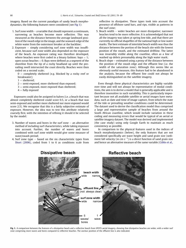
imagery. Based on the current paradigm of sandy beach morpho-dynamics, the following features were considered (see Fig 1):

1. Surf zonewidthe a variable that should represent a continuum,narrowing as beaches become more reflective. This wasmeasured as the distance between the average landward posi-tionof the swash edge in the image, and the seaward-edgeof thewhite water from the outermost breaker at the backline;

2. Exposure e simply considering surf zone width was insuffi-cient, because surf zone width also depended on the exposureof the beach. An exposure rating was therefore developed,where beaches were first coded in a binary fashion: bays ¼ 1;open ocean beaches ¼ 0. Bays were defined as a segment of theshoreline from the tip of a rocky headland up until the pre-vailing swell intersected the coast directly. Beaches were thencoded on a second scale;

0 ¼ completely sheltered (e.g. blocked by a rocky reef orbreakwater);1 ¼ sheltered;2 ¼ semi-exposed, more sheltered than exposed;3 ¼ semi-exposed, more exposed than sheltered;4 ¼ fully exposed

Exposures could also be assigned in halves (i.e. a beach that wasalmost completely sheltered could score 0.5, or a beach that wassemi-exposed and neither more sheltered nor more exposed wouldscore 2.5). We recognise that this is a fairly subjective estimate ofexposure. However, the idea was to test this attribute relativelycoarsely first, with the intention of refining it should it be selectedby the model:

3. Number of waves and bores in the surf zone e an alternativemethod of including surf characteristics, while taking exposureinto account. Further, the number of waves and borescombined with surf zone width would give some measure ofwave/swash period;

4. Surf zone type e based on the six characteristic types fromShort (2006), coded from 1 to 6 as conditions scale from

Fig. 1. A comparison between the features of a dissipative beach and a reflective beach fromzone comprising more waves and bores compared to reflective beaches. The unclear positi

reflective to dissipative. These types took into account thepresence of offshore sand bars, and rips, visible as patterns inthe surf zone;

5. Beach width e wider beaches are more dissipative; narrowerbeaches tend to be more reflective. It is acknowledged that notall the imagery was taken at spring low tide, and that there arecurrently no official shapefiles of the national high or lowwatermarks. The best estimate of intertidal beach width was thus thedistance between the portion of the beach site with the lowestposition of the swash, and the estimated driftline. The latterwas invariably visible along the coastline, often as a line ofwashed up debris presumably along the high water mark;

6. Beach slope e estimated using a proxy of the distance betweenthe position of the swash edge and the effluent line (i.e. thewidth of the saturation zone). Although this seems like anobviously useful measure, this feature had to be abandoned inthe analysis, because the effluent line could not always beeasily distinguished on the satellite imagery.

Even though these physical characteristics are highly variableover time and will not always be representative of modal condi-tions, the aim is to derive a model that is generally applicable and istherefore insensitive to such variability. This is particularly impor-tant because not all available satellite or aerial images have meta-data, such as date and time of image capture, from which the stateof the tide or prevailing weather conditions could be determined.The dataset used to derive the classification model thus compriseda large and representative sample of beaches from around theSouth African coastline, which would include variation in thesecoding and measuring errors that would be typical of an aerial orsatellite imagery dataset. The model was derived and implemented(the case study) using only Google Earth to maintain as muchconsistency as possible.

In comparison to the physical features used in the indices ofbeach morphodynamics (below), the only features that are notconsidered specifically are wave height and sand grain size (sedi-ment fall velocity (in cm s�1) is a direct function of sand grain sizeand hence an alternative measure of the same variable (Gibbs et al.,

SPOT5 aerial imagery, showing that dissipative beaches are wider, with a wider surfon of the effluent line is also indicated.

1.8 2.0 2.2 2.4 2.6 2.8 3.0 3.2 3.4

10Log sand grain size (µm)

0.6

0.8

1.0

1.2

1.4

1.6

1.8

b

c

2.0

goL01

epols)/1(

1.8 2.0 2.2 2.4 2.6 2.8 3.0 3.2 3.4

Log10 sand grain size (µm)

0.8

1.0

1.2

1.4

1.6

1.8

2.0

2.2

2.4

goL01

(htdi

whcaeb

)m

0.8 1.0 1.2 1.4 1.6 1.8 2.0 2.2 2.4

Log10 beach width (m)

0.6

0.8

1.0

1.2

1.4

1.6

1.8

2.0

goL01

epols)/1(

a

Fig. 2. Significant correlations between (a) (log) sand grain size (mm) and (log 1/)beach slope; and (b) (log) sand grain size (mm) and (c) (log 1/) beach slope with (log)beach intertidal width (m). (Data used in this analysis are taken from our collateddatabase of previously sampled beaches in southern Africa).

L. Harris et al. / Estuarine, Coastal and Shelf Science 92 (2011) 78e89 81

1971)). The beach morphodynamic indices are represented by thefollowing formulae: dimensionless fall velocity (U; Gourlay, 1968),which measures the ability of waves to move sand (Wright andShort, 1984); the beach state index (BSI), which measures theability of waves and tides to move sand (Defeo and McLachlan,2005); the beach index (BI), which allows beaches of differentwidths to be compared (McLachlan and Dorvlo, 2005); the beachdeposit index (BDI), which measures the slope and sand propertiesof a beach (Soares, 2003).

U ¼ HbWs � Tw

(1)

BSI ¼ U� TR (2)

BI ¼ log10

�Mz � TR

S

�(3)

BDI ¼�1S

���

aMz

�(4)

Where: Hb ¼ wave height (cm); Ws ¼ sediment fall velocity(cm s�1); Tw ¼ wave period (s); TR ¼ tide range (m); Mz ¼ sandgrain size (mm; 4 þ 1 for BI, to avoid negative values); S ¼ averageintertidal slope; a¼ 1.03125 mm and is the median grain size of thesediment classification scheme.

In our opinion, excluding wave height and sand grain size doesnot weaken the classification. Consider that on any day there area number of factors that could influence the size of waves. Byimplication, snapshot readings of wave height are a weakness inthose formulations dependent on that value. With this in mind, weconsidered it an acceptable omission in this study. Sand grain size isa far more stable, important driver of sandy beach morphodynamictypes, but this is not applicable for inclusion in the classificationmodel because it cannot be measured or observed from aerialimages. Sand grain size is known to be significantly correlated withbeach slope (Fig. 2a: r¼�0.6381, p< 0.01, n¼ 174; see also Bascom,1951; McLachlan and Dorvlo, 2005; McLachlan and Brown, 2006),but slope is also not a feasible feature to measure from two-dimensional imagery. However, both slope (Fig. 2b: r ¼ 0.7533,p < 0.01, n ¼ 187) and sand grain size (Fig. 2c: r ¼ �0.4869,p < 0.001, n ¼ 195) are significantly correlated with beach width,which can be measured off an aerial image. Although these corre-lations are weak, they show that our selected proxies reflect at leastsome aspects of these two variables that could not be included inthe classification routine.

2.1.2. Statistical application: conditional inference treesThere are a number of statistical applications in studies of

ecology that can be used to define meaningful categories or groupsfrom a single dataset comprising multiple input variables. Of these,we selected conditional inference trees, a type of non-parametricregression tree. We made this selection because input variables cancomprise all kinds of data (nominal, ordinal, numeric, censored andmultivariate), and do not have to satisfy any assumptions ofnormality or homoscedacity (Hothorn et al., 2006, 2007, 2009;Olden et al., 2008).

Furthermore, conditional inference trees are extremely flexiblein identifying statistically significant patterns (both linear andnon-linear) from potentially confounded or interacting predictorvariables because they classify samples (beaches) according toa hierarchical set of quantitative criteria using pragmatic selectionsfrom all available input variables (Venables and Ripley, 2002; Zuuret al., 2007). This has the additional benefit that samples (beaches)

can be explicitly classified on the basis of quantitative, statisticallysignificant metrics.

The underlying analysis relies on recursive binary partitioningto estimate regression relationships by assessing groups of data(nodes) for independence between input variables and theresponse (Hothorn et al., 2009). Where input variables (single ormultiple) are associated with the response, the response variable is

L. Harris et al. / Estuarine, Coastal and Shelf Science 92 (2011) 78e8982

divided (partitioned) at a specific value of the most significantlyassociated predictor (as indicated by p-values) in a binary fashion toproduce two child nodes (classes of the response variable). Thisprocess is repeated recursively for each node until it can no longerbe split into groups that differ significantly. This is then defined asa terminal node, or a leaf of the tree. Predefining the stoppingcriterion (e.g. only allowing splits where p < 0.05, or defininga minimum number of samples in a node) can avoid having toprune the tree at a later stage by preventing overfitting of the data(Hothorn et al., 2009). Bonferroni-adjusted p-values at a ¼ 0.05were used in this study to control tree growth, thus accounting forbiases that may be introduced by multiple hypothesis tests.

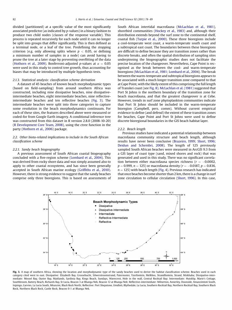
2.1.3. Statistical analysis: classification scheme derivationA dataset of 45 beaches of known beach morphodynamic types

(based on field-sampling) from around southern Africa wasconstructed, including nine dissipative beaches, nine dissipative-intermediate beaches, eight intermediate beaches, nine reflective-intermediate beaches and ten reflective beaches (Fig. 3). Theintermediate beaches were split into three categories to capturesome resolution in the beach morphodynamics continuum. Foreach of these sites, the features described above were measured orcoded-for from Google Earth imagery. A conditional inference treewas constructed from this dataset in R version 2.8.0 (2008-10-20)(R Development Core Team, 2008), using the ctree function in theparty (Hothorn et al., 2006) package.

2.2. Other biota-related implications to include in the South Africanclassification scheme

2.2.1. Sandy beach biogeographyA previous assessment of South African coastal biogeography

concluded with a five-region scheme (Lombard et al., 2004). Thiswas derived from rocky shore data and was simply assumed also toapply to other coastal ecosystems, and has since been generallyaccepted in South African marine ecology (Griffiths et al., 2010).However, there is strong evidence to suggest that the sandy beachescomprise only three bioregions. This is based on assessments of

Fig. 3. A map of southern Africa, showing the location and morphodynamic type of the scategory cited west to east. Dissipative: Elizabeth Bay, Grossebucht, Silwerstroomstrand,mediate: Mossel Bay, Oyster Bay, Maitlands, Sardinia Bay, Kings Beach, Sundays, WavecrSouthbroom, Battery Beach, Richards Bay, St Lucia, Beacon 3 at Bhanga Nek, Beacon 12 at BhIsipingo, Garvies, La Lucia South, Mtunzini, Black Rock North; Reflective: Port Shepstone, UmRock, Northern Black Rock, Castle Rock, Beacon 0-1 at Bhanga Nek.

South African intertidal macrofauna (McLachlan et al., 1981),shorebird communities (Hockey et al., 1983) and, although theirdistribution extends beyond the surf zone to the continental shelf,coastal fish (Turpie et al., 2000). These three bioregions includea cool-temperate west coast, a warm-temperate south coast anda subtropical east coast. The boundaries between these bioregionsare difficult to define because they are transition zones rather thandiscrete breaks, and often the spatial distribution of sampling sitesunderpinning the biogeographic studies does not facilitate theprecise location of the changeover. Nevertheless, Cape Point is rec-ognised as the break between the cool- and warm-temperatebioregions (McLachlan et al., 1981; Lombard et al., 2004). The breakbetween thewarm-temperate and subtropical bioregions appears tobe associated with a much longer transition zone compared to thatat Cape Point,with the likelyextent of this comprising the full lengthof Transkei coast (see Fig. 8). McLachlan et al. (1981) suggested thatPort St Johns is the northern boundary of the transition zone forbeach macrofauna, and that the greatest changeover is at Cebe.However, trends in surf zone phytoplankton communities indicatethat Port St Johns should be included in the warm-temperatebioregion (Campbell, pers. comm). Without current empiricalevidence to define (and defend) the extent of these transition zonesfor beaches, Cape Point and Port St Johns were used to definediscrete bioregional boundaries in the GIS beach habitat layer.

2.2.2. Beach lengthPrevious studies have indicated a potential relationship between

macrofauna community structure and beach length, althoughresults have never been conclusive (Brazeiro, 1999; Short, 1996;Deidun and Schembri, 2008). The length of 125 previouslysampled South African beaches were measured in ArcGIS 9.3 froma GIS layer of coast type (sand, mixed shores and rock) that wasgenerated and used in this study. There was no significant correla-tion between either macrofauna species richness (r ¼ �0.0002,p ¼ 0.999, n ¼ 125) or macrofauna density (r ¼ �0.0187, p ¼ 0.836,n ¼ 125) with beach length (Fig. 4). Previous research has indicatedthatoncebeachesbecomeshorter than2km, there is a change in surfzone circulation to cellular circulation (Short, 1996). In this case,

andy beaches used to derive the habitat classification scheme. Beaches used in eachPaternoster, Yzerfontein, Melkbos, Strandfontein, Strand, Msikhaba; Dissipative-inter-est, Hole in the wall, Central Rocktail Bay; Intermediate: Huisklip, Marie’s Cottage,anga Nek; Reflective-intermediate: Milnerton, Annerley, Doonside, Amanzimtoti South,dloti, Blythedale, La Lucia, Southern Rocktail Bay, Northern Rocktail Bay, Southern Black

0 10 20 30 40 50 60

Beach length (km)

0

5

10

15

20

25

30

ssenhcirseicepS

0 10 20 30 40 50 60

Beach length (km)

0

200

400

600

800

1000

1200

1400

m.oN(

ytisnedanuaforca

M2-)

a

b

Fig. 4. There is no correlation between beach length (km) and either (a) macrofauna species richness or (b) macrofauna density (no. m�2) (n ¼ 125).

L. Harris et al. / Estuarine, Coastal and Shelf Science 92 (2011) 78e89 83

“longshore flow dominates within the embayment, with strongseaward-flowing topographic rips occurring at one or both ends ofthe embayment” (McLachlan and Brown, 2006). An independentstudy showed that, taking morphodynamics into account, macro-fauna species richness decreases once beaches become shorter than2 km (Brazeiro,1999). Analysis of the beaches less than 2 km long inour database did not support this finding, and neither species rich-ness (r ¼ 0.0773, p ¼ 0.659, n ¼ 35) nor macrofaunal density(r¼�0.0300, p¼0.864,n¼35)was significantly correlated tobeachlength.Howbeach length isdefinedwhen interspersedwithpatchesof mixed shores as opposed to more obvious boundaries such asrocky headlands, however, is a debatable point. Given the currentlack of evidence, beach length was disregarded as a factor.

2.2.3. Estuarine beachesTherearedifferences inmacrofaunal communitieswith increasing

distance fromestuaries (SchoemanandRichardson, 2002; Lercari andDefeo, 2006; Ortega-Cisneros, 2009). This is largely attributed tosalinity changes,with lower salinities around themouths of estuaries,and varying tolerances of macrofauna to this. Furthermore, fortemporarily open-closed estuaries, the sandy beach in front of themouth is not stable (or rather, less stable than already dynamic sandybeaches). This area experiences periodic scouring of the sand as theestuarybreaches,floodingof thebeach face, and thus rapidchanges inthe localised salinity, all with implications for beach biota. For thisreason, distinguishing between estuarine and purely sandy beacheswas considered necessary. Beaches were coded such that, if the

L. Harris et al. / Estuarine, Coastal and Shelf Science 92 (2011) 78e8984

estuaryhad toflood, theportionof sandybeach thatwouldbefloodedwas recorded as estuarine.

3. Results

3.1. Classification model

The predictive classification tree (with only significant parti-tioning) was based solely on beach width (Fig. 5). None of the otherinput variables were stronger, more significant predictors of beachmorphodynamic type. However, the model could not distinguishbetween intermediate and reflective-intermediate beaches becausethere was no significant split between these two states (formicrotidal beaches in South Africa). This forced the merging ofthese categories into a single “intermediate beach type” category.When the tree was reconstructed after this merger, it made no

≤ 66

BWidthp < 0.001

2

≤ 28.79 > 28.79

Node 3 (n = 10)

1 2 3 4 50

0.2

0.4

0.6

0.8

1

BWidp = 0.0

4

≤ 47.04

Node 5 (n = 28)

1 2 3 4 50

0.2

0.4

0.6

0.8

1

Fig. 5. Conditional inference tree showing the significant (p < 0.05) groupings of sandy beachNode 6 ¼ dissipative-intermediate beaches; Node 7 ¼ dissipative beaches. The bar chartsintermediate; 3 ¼ intermediate; 4 ¼ reflective-intermediate; 5 ¼ reflective) falling in that

difference to the tree structure or cut-off values. Based on thisclassification model, the estimated minimum beach width for eachof the beach morphodynamic types is 64.11 m for dissipative bea-ches, 47.04 m for dissipative-intermediate beaches, 27.49 m forintermediate beaches, and any beach narrower than 27.49 m isreflective (Fig. 5).

3.2. Classification model verification

The model was verified by creating a confusion matrix fora separate set of 28 beaches of a variety of known (from field-sampling) beach morphodynamic types (Fig. 6) and that were notpreviously used in the model derivation. The accuracy of modelpredictions was 75%. The beaches that were misclassified hadbeach widths close to those of the breaks between the four cate-gories. In all but one case, these misclassified beaches were

BWidthp < 0.001

1

.31 > 66.31

th02

> 47.04

Node 6 (n = 15)

1 2 3 4 50

0.2

0.4

0.6

0.8

1Node 7 (n = 17)

1 2 3 4 50

0.2

0.4

0.6

0.8

1

es based on beach width. Node 3 ¼ reflective beaches; Node 5 ¼ intermediate beaches;indicate the proportion of each of the beach types (1 ¼ dissipative; 2 ¼ dissipative-node.

Fig. 6. A map of southern Africa, showing the location and known morphodynamic type of the sandy beaches used to verify the habitat classification scheme. Beaches cited fromwest to east: Dernburg Bay, Dwaskersbos, Slipper Bay, Stompneusbaai, Veldrift, Blouberg, Transhex site C, Transhex site C1, Transhex site FI2, Muizenberg, Macassar, Cotton, Still Bay,Sedgefield, Plettenberg Bay, Jeffreys Bay, Van Staadens, Boknes, Port Alfred, Anstees, Thompsons Bay Ballito, Mlalazi, Mapelane launch site, Mapelane control site, Cape Vidal controlsite, Cape Vidal launch site, Sodwana, Island Rock control site, Island Rock launch site.

L. Harris et al. / Estuarine, Coastal and Shelf Science 92 (2011) 78e89 85

predicted to be in a category that was adjacent to the observedcategory. For example, dissipative-intermediate beaches wererecorded as dissipative, or as intermediate.

Beaches with a beach width that is approximately 5 m eitherside of the cut-off value defining the breaks between groups (i.e.a 10-m “transition band” between categories) evidently requirecoding of other habitat features in addition to beach width forcorrect classification. The misclassified beaches were thus rerunthrough the classification tree algorithms, but no significant nodeswere identified from this smaller dataset. It was observed, however,that a more applied consideration of surf zone type corrected six ofthe eight previous misclassifications, and resulted in a w20%improvement of the overall model accuracy (to 93%). Application ofsurf zone type in the classification model is described below.

Beaches with a beach width that fell into one of the threetransition zones (between the four categories) could be classified asone of two possible beach morphodynamic types. One of these ismore reflective and the other, more dissipative. For example,intermediate beaches are more reflective than dissipative-inter-mediate beaches. For the transitions involving the extreme SouthAfrican beach states, dissipative beaches vs. dissipative-interme-diate, and reflective beaches vs. intermediate, the extreme surfzone types (dissipative or reflective) had to be present to force thebeach into the respective extreme category. If this was not the case,the alternative, more intermediate state of the two options in thetransition was selected. For the break between intermediate anddissipative-intermediate beaches: if the surf zone was of a morereflective nature (types 1e3 sensu Short (2006), see Section 2.1.1),then the intermediate category was selected; conversely if the surfzone was of a more dissipative nature (types 4-6 sensu Short(2006), see Section 2.1.1), then the dissipative-intermediate typewas selected.

Given the 93% accuracy of the classification model, it isconsidered a tool with sufficient predictive power to classify theSouth African sandy beaches from a purely desktop approach.Finally, the “predict” and “verify” datasets were combined (total of73 beaches), and the conditional inference treewas rerun in R, withthe intent that the larger dataset would inform a more accurateestimate of the cut-off beach width values that define the breaksbetween categories. However, this final model (Fig. 7) was nearly

identical to the original classification tree (Fig. 5): the cut-off valuesdescribing the breaks differed by only 0e2.2 m; a range which iswell within the 5-m transition band on each side of the breaks. Thisresult further confirmed the validity of our approach.

3.3. Final habitat classification scheme and applicationto the South African coastline

3.3.1. Mapping methodologyThe final classification scheme of South African sandy beaches

involved four morphodynamic types (dissipative, dissipative-intermediate, intermediate and reflective) nested within two beachtypes (sandy or estuarine), in turn nested within three biogeo-graphic regions (cool-temperate west coast, warm-temperatesouth coast, subtropical east coast), yielding 24 different beachhabitats. These were classified and mapped in ArcGIS 9.3 accordingto the following rules (note that rock and mixed shores were alsocoded for and mapped, and that the shapefile was digitized ontoSPOT5 satellite imagery):

1. If the intertidal beach width measured on Google Earth was:a. >66 m ¼ dissipative beach;b. 47e66 m ¼ dissipative-intermediate beach;c. 29e47 m ¼ intermediate beach;d. <29 m ¼ reflective beach;

2. Beaches with a beach width that fell in the 10-m transitionzone between the categories (i.e. beach width ¼ 61e71 m;42e52m; or 24e34m) also required an assessment of the localsurf zone:a. If the surf zone category tended towards being reflective,

the more reflective of the two possible morphodynamictypes in the transition zone was selected and assigned tothe beach;

b. If the surf zone category tended towards being dissipative,the more dissipative of the two possible morphodynamictypes in the transition zone was selected and assigned tothe beach;

3. Classification was not pedantic: breaks were made alongshoreonly where the beach morphodynamic type made a consistent

Fig. 7. Conditional inference tree showing the significant (p < 0.05) groupings of sandy beaches based on beach width. Node 3 ¼ reflective beaches; Node 5 ¼ intermediate beaches;Node 6 ¼ dissipative-intermediate beaches; Node 7 ¼ dissipative beaches. The bar charts indicate the proportion of each of the beach types (1 ¼ dissipative; 2 ¼ dissipative-intermediate; 3 ¼ intermediate (combined intermediate and reflective-intermediate); 5 ¼ reflective) falling in that node.

L. Harris et al. / Estuarine, Coastal and Shelf Science 92 (2011) 78e8986

change. Furthermore, alongshore units were coded only if theywere longer than the beach was wide;

4. A beach was coded as estuarine where, if the estuary/rivermouth breached, the beach would be scoured out, or floodedwith estuarine water;

5. Superimposed on the above were the empirically derivedbiogeographic zones;a. Subtropical: Ponta do Ouro to Port St Johns;b. Warm-temperate: Port St Johns to Cape Point;c. Cool-temperate: Cape Point to Orange River mouth

3.3.2. South African shorelineAlthough sand, mixed shores and rock are represented in

approximately equal proportions along the national shoreline,sandy beaches are the dominant coast type in South Africa. Based

on the classifications describe above, more than 80% of thesebeaches are of the intermediate morphodynamic state (interme-diate and dissipative-intermediate combined), with dissipative-intermediate beaches being most common. This is so, becausenearly three quarters of the south coast (the bioregion thataccounts for half the national coastline) comprises dissipative-intermediate beaches. The two morphodynamic extremes, dissi-pative and reflective beaches, make up only a small proportion ofthe coastline (w12% and w7%, respectively). This is partly becausethey are both truly represented in only two of the three bior-egions e there is virtually no dissipative beach along the east coast(<2 km of 671.23 km), and hardly any reflective beach on the southcoast (<4 km of 1544.23 km). From a conservation planningperspective, it is an important result that the distribution of beachmorphodynamic types is partly influenced by geography (Table 1,Fig. 8).

Table 1Synopsis of the South African coastline, citing the lengths of the coast types and sandy beach morphodynamic types per bioregion, and for the national shoreline. Values aregiven in km, and as a percentage of the total sand beaches per region in curly brackets {}, of the bioregional coastline in round brackets (), and of the national coastline in squarebrackets [], where appropriate.

Region Coast typesa Sandy beachesb

Location Length Category Length Morphodynamic type Length

West coast bioregion 897.33 [28.83] Sand 315.61 (35.17) [10.14] Dissipative 58.73 {18.91} (6.54) [1.89]Mixed 289.32 (32.24) [9.29] Dissipative-Intermediate 109.74 {35.33} (12.23) [3.53]Rock 285.53 (31.82) [9.17] Intermediate 109.17 {35.15} (12.17) [3.51]Other 6.87 (0.77) [0.22] Reflective 32.96 {10.61} (3.67) [1.06]

South coast bioregion 1544.23 [49.61] Sand 527.92 (34.19) [16.96] Dissipative 74.41 {15.27} (4.82) [2.39]Mixed 478.86 (31.01) [15.38] Dissipative-Intermediate 342.27 {70.26} (22.16) [11.00]Rock 530.29 (34.34) [17.04] Intermediate 66.54 {13.66} (4.31) [2.14]Other 7.16 (0.46) [0.23] Reflective 3.96 {0.81} (0.26) [0.13]

East coast bioregion 671.23 [21.56] Sand 360.88 (53.76) [11.59] Dissipative 1.86 {0.56} (0.28) [0.06]Mixed 235.63 (35.10) [7.57] Dissipative-Intermediate 118.92 {35.68} (17.71) [3.82]Rock 72.69 (10.83) [2.34] Intermediate 166.91 {50.08} (24.87) [5.36]Other 2.03 (0.30) [0.07] Reflective 45.61 {13.68} (6.79) [1.47]

National coastline 3112.79 [100] Sand 1204.41 [38.69] Dissipative 135.01 {11.94} [4.34]Mixed 1003.80 [32.25] Dissipative-Intermediate 570.93 {50.48} [18.34]Rock 888.51 [28.54] Intermediate 342.62 {30.29} [11.01]Other 16.07 [0.52] Reflective 82.52 {7.30} [2.65]

a Sand includes: sandy beach; estuarine beach. Mixed includes: all forms of mixed shores. Rock includes: boulder beach, breakwater, cliff, cliff with rocky base, estuarineboulder beach, estuarine rock, estuarine mouth boulder beach, rock. Other includes: harbour mouth, estuary/river mouth.

b Values exclude estuarine beaches.

L. Harris et al. / Estuarine, Coastal and Shelf Science 92 (2011) 78e89 87

4. Discussion

4.1. A successful tool

The methodology developed here for mapping sandy beachesremotely was shown to be a very successful tool. Further, it has thepotential to be applied to other regional or national coastlines withease. It must be borne in mind, however, that the South Africancoastline is uniformly microtidal (tide range of 1.6e1.7 m). Thus thebeach widths used to define the morphodynamic types in this casestudy will not be necessarily applicable to meso- or macrotidalsystems where shorelines may be up to several hundred metreswide at low tide. It is recommended that the model is re-trainedbased on country- or region-specific data, and preferably ground-truthed locally, before its application.

One issue that was not explored here is the well-knowndynamic nature of sandy beaches. Sandy beaches with low-lyingrocks that become periodically exposed and covered during natural

Fig. 8. A map of the South African coastline (between the Orange River mouth and Pobiogeographic breaks (solid stars) mark the boundaries between the cool-temperate westemperate south coast and the subtropical east coast (Port St Johns). The extent of the likely

erosioneaccretion cycles, for example, may be more appropriatelycoded as “intermediate sandy beach, temporary mixed shore”.Although mapping at this resolution was not our aim, the option toinclude a temporal component does exist if the model is applied tomultiple sets of images. This highlights one of the tremendousbenefits of mapping beach morphodynamic types remotely ratherthan from field-based assessments: if there is sufficiently clearhistorical imagery, beach morphodynamic types can even bemapped for periods long before the morphodynamics paradigmexisted.

4.2. The South African shoreline

The most unexpected result was the geographic distribution ofbeach morphodynamic types along the South African coastline.Previous work in Northern Ireland showed that underlying geologywas the most important determinant of the spatial distribution ofbeach morphodynamic types (Jackson et al., 2005). In light of the

nto do Ouro) showing the spatial distribution of beach morphodynamic types. Thet coast and the warm-temperate south coast (Cape Point), and between the warm-transition zone (Transkei) between the latter two bioregions is indicated (open stars).

L. Harris et al. / Estuarine, Coastal and Shelf Science 92 (2011) 78e8988

results in our study, their finding could very likely apply to SouthAfrica as well. Furthermore, while not captured specifically in thenumerical data, general shoreline morphology is also geographi-cally distinct per each bioregion.

The South African west coast is an extremely heterogeneousportion of the national coastline, with stark contrasts betweenrugged rocky cliffs and long sandy beaches, extremely sheltered,deep bays and highly exposed, straight, open coasts. There areapproximately equal proportions of rock, mixed shores and sandybeaches in this bioregion. The west coast beaches are wave-domi-nated andmicrotidal, with representation from the full spectrum ofbeach morphodynamic types. In southern Western Cape, rockysections are interspersed with small reflective and intermediatebeaches. The long beaches in northern Western Cape primarilycomprise dissipative and dissipative-intermediate beaches. Thecoastline is predominantly rocky in the Northern Cape, becomingintermediate and reflective towards the Orange River. Thus, overall,the dominant beach morphodynamic types in this bioregion aredissipative-intermediate and intermediate beaches.

The largest coastal bioregion in South Africa is the south coast,making up nearly half of the national shoreline. It comprisesnumerous, consecutive log-spiral (half-heart shaped) bays, e.g.Vlees Bay, Mossel Bay, Plettenberg Bay, Oyster Bay, St Francis Bay,and Algoa Bay, with exposure increasing from west to east withineach bay. These log-spiral bays are generally interspersed with cliffsor rocky stretches of coastline. In most of these cases, sand is blownover the rocky headland through mobile dunes, in the form ofa series of headland-bypass dune systems. In cases where thesedunes have been stabilised, and sandmovement has been retarded,the beaches inside the bay are eroding, e.g. St Francis Bay (La Cockand Burkinshaw, 1996). The beach morphodynamic type in thisregion is almost exclusively (w70%) dissipative-intermediate, withequal proportions of dissipative and intermediate beaches (w15%each) comprising the rest of the shoreline. There are hardly anyreflective beaches in the region. Interestingly, the south coast hasthe longest continuous stretches of both sand (Alexandria) and ofrock (Tsitsikamma). Of particular significance is the Alexandriadune field, just north of Port Elizabeth in Algoa Bay. At 50 km longand 2.1 km wide, and with dunes over 150 m in height, it is one ofthe largest active coastal dune fields in the world (McLachlan et al.,1982).

In contrast to the long sandy beaches along the south coast, theTranskei coast (transition between the south- and east-coastbioregions) is predominantly rock or cliff, interspersed with pocketand embayed beaches that are invariably associated with estuaries.These beaches tend to be intermediate to reflective. The beachesbetween Port Edward and Durban are predominantly reflective orintermediate and rocky, with numerous small temporary open-closed estuaries. Further to the north, beaches become more inter-mediate/dissipative-intermediate and estuaries become sparser,with the Tugela River and the two estuarine lake systems of Kosi Bayand St Lucia of significance in this area. There are virtually no trulydissipative beaches along the east coast. While not specificallyprotecting sandy beaches, the northern-most 200 km of the SouthAfrican east coast comprises the iSimangaliso Wetland Park, whichincludes the Maputaland and St Lucia Marine Reserves. It is of notethat thebeaches in thePark are theonly turtle nestinggrounds in thecountry.

In the context of our objectives for generating this shapefile (forconservation planning), this asymmetric spatial distribution ofbeach types per bioregion has significant implications for habitatrepresentation in a conservationplan. This is particularly true for thedissipative and reflective beaches that comprise less than 1% of theeast and south coast, respectively. As a result, a beach that appears tobe a comparatively inferior candidate site for conservation priority

may actually rank as highly irreplaceable because it is a uniquehabitat with regionally rare species assemblages.

The spatial trends in beachmorphodynamic types and shorelinemorphology also raises ecological questions. For example, it hasimplications for the potential isolation of populations on regionallyrare beach types, and thus the heightened vulnerability of thesepopulations to threats such as coastal squeeze (Dugan et al., 2008)and/or high-impact erosion events like extreme storms (Brown andMcLachlan, 2002; Smith et al., 2007; Schlacher et al., 2008; Defeoet al., 2009). This is particularly important considering thebiogeographic distribution of the fauna (McLachlan et al., 1981):some are present in only a single bioregion and have clear habitatpreferences as per the swash exclusion hypothesis (McLachlanet al., 1993). Our current understanding of population connec-tivity among beaches is fairly speculative (Caddy and Defeo, 2003;Defeo andMcLachlan, 2005); thus representing shorelines spatiallyon a regional or national scale has potential application in inter-rogating such issues.

4.3. Potential applications

The number of GIS-based ecological applications available toresearchers is rapidly escalating. Having a digitally representedshoreline, mapped per beach morphodynamic type, thus opens upa myriad of analyses at a range of spatial scales. These range intechnicality from the simplest of exercises, to extremely complex,multivariate problems. For example, the shapefile could form partof a GIS-based decision-support system where certain activities(e.g. beach driving or coastal development) are discouraged orbanned from the beach morphodynamic types that show greatersensitivity to associated impacts. A slightly more advanced analysiscould be large-scale quantification of ecosystem processes, likewater filtration, for example. In this case, a few simple experimentscould be extrapolated up to a regional or national scale using beachmorphodynamic type as a proxy for sand grain size and swashclimate. More sophisticated applications include SCP exercises,where the beach morphodynamic type shapefile is only one ofa number of input variables. As more spatial analyses and tech-niques become available, the number of potential applications forthis tool motivate strongly for its implementation.

5. Conclusions

This study successfully derived and implemented a novelmethodology whereby sandy beach morphodynamic types can bemapped digitally. Its highly-adaptable nature allows for country- orregion-specific training of the model, which means that it could beapplied across a range of conditions world-wide. Where modeltraining can be coupled with local ground-truthing, the model canbe applied with confidence. The number of available applicationsonce a beach morphodynamics shapefile has been created isendless and allows for the interrogation of numerous unexploredquestions in beach ecological theory.

Acknowledgements

The authors thank Anton McLachlan and two anonymousreviewers for their comments on an earlier version of the manu-script, and Eileen Campbell for discussions relating to this study.Funding was provided by the South African National BiodiversityInstitute, as part of the National Biodiversity Assessment 2010. TheNational Research Foundation and Nelson Mandela MetropolitanUniversity provided financial support for LH.

L. Harris et al. / Estuarine, Coastal and Shelf Science 92 (2011) 78e89 89

References

Banks, S.A., Skilleter, G.A., 2002.Mapping intertidal habitats andanevaluationof theirconservation status inQueensland, Australia. Ocean andCoastalManagement 45,485e509.

Banks, S.A., Skilleter, G.A., 2007. The importance of incorporating fine-scale habitatdata into the design of an intertidal marine reserve system. Biological Conser-vation 138, 13e29.

Bascom, W.M., 1951. The relationship between sand size and beach slope. Trans-actions of the American Geophysical Union 32, 866e874.

Brazeiro, A., 1999. Community patterns in sandy beaches of Chile: richness,composition, distribution and abundance of species. Revista Chilena De HistoriaNatural 72, 93e105.

Brown,A.C.,McLachlan, A., 2002. Sandyshore ecosystems and the threats facing them:some predictions for the year 2025. Environmental Conservation 29, 62e77.

Caddy, J.F., Defeo, O., 2003. Enhancing or restoring the productivity of naturalpopulations of shellfish and other marine invertebrate resources. FAO FisheriesTechnical Paper 1, 159 (IV).

Coombes, E.G., Jones, A.P., Sutherland, W.J., 2009. The implications of climatechange on coastal visitor numbers: a regional analysis. Journal of CoastalResearch 25, 981e990.

Davenport, J., Davenport, J.L., 2006. The impact of tourism and personal leisuretransport on coastal environments: a review. Estuarine Coastal and ShelfScience 67, 280e292.

Defeo, O., McLachlan, A., 2005. Patterns, processes and regulatory mechanisms insandy beach macrofauna: a multi-scale analysis. Marine Ecology Progress Series295, 1e20.

Defeo, O., McLachlan, A., Schoeman, D.S., Schlacher, T.A., Dugan, J., Jones, A.,Lastra, M., Scapini, F., 2009. Threats to sandy beach ecosystems: a review.Estuarine, Coastal and Shelf Science 81, 1e12.

Deidun, A., Schembri, P.J., 2008. Long or short? Investigating the effect of beachlength and other environmental parameters on macrofaunal assemblages ofMaltese pocket beaches. Estuarine Coastal and Shelf Science 79, 17e23.

Dugan, J.E., Defeo, O., Jaramillo, E., Jones, A.P., Lastra, M., Nel, R., Peterson, C.H.,Scapini, F., Schlacher, T.A., Schoeman, D.S., 2010. Give beach ecosystems theirday in the sun. Science 329, 1146.

Dugan, J., Hubbard, D.M., Rodil, I.F., Revell, D., Schroeter, S., 2008. Ecological effectsof coastal armouring on sandy beaches. Marine Ecology 29, 160e170.

Gibbs, R.J., Matthews, M.D., Link, D.A., 1971. The relationship between sphere sizeand settling velocity. Journal of Sedimentary Research 41, 7e18.

Gladstone, W., Alexander, T., 2005. A test of the higher-taxon approach in theidentification of candidate sites for marine reserves. Biodiversity and Conser-vation 14, 3151e3168.

Gourlay, M.R., 1968. Beach and Dune Erosion Tests. Delft Hydraulics Laboratory.Report No.M935/M936.

Griffiths, C.L., Robinson, T.B., Lange, L., Mead, A., 2010. Marine biodiversity in SouthAfrica: an evaluation of current states of knowledge. PLoS ONE 5, 1e13.

Hockey, P.A.R., Siegfried, W.R., Crowe, A.A., 1983. Ecological structure and energyrequirements of the sandy beach avifauna of southern Africa. In: McLachlan, A.,Erasmus, T. (Eds.), SandyBeachesasEcosystems.DrWJunk,TheHague,pp. 501e506.

Hothorn, T., Hornik, K., Strobl, C., Zeileis, A., June 2009. Package ’party’. PackageReference Manual for Party Version 0.9-998 16, 37.

Hothorn, T., Hornik, K., Zeileis, A., 2006. Unbiased recursive partitioning: a condi-tional inference framework. Journal of Computational and Graphical Statistics15, 651e674.

Hothorn, T., Zeileis, A., Hornik, K., 2007. Let’s have a party! An open-source toolboxfor recursive partytioning. In: Research Report Series. Department of Statisticsand Mathematics, Wirtschaftsuniversitat Wien, pp. 1e5.

Howes, D., 2001. BC Biophysical Shore-zone Mapping System - A SystematicApproach to Characterize Coastal Habitats in the Pacific Northwest. PugetSound Research.

Jackson, D.W.T., Cooper, J.A.G., del Rio, L., 2005. Geological control of beach mor-phodynamic state. Marine Geology 216, 297e314.

La Cock, G.D., Burkinshaw, J.R., 1996. Management implications of developmentresulting in disruption of a headland bypass dunefield and its associated river,Cape St Francis, South Africa. Landscape and Urban Planning 34, 373e381.

Lercari, D., Defeo, O., 2006. Large-scale diversity and abundance trends in sandybeach macrofauna along full gradients of salinity and morphodynamics. Estu-arine Coastal and Shelf Science 68, 27e35.

Leslie, H., Ruckelshaus, M., Ball, I.R., Andelman, S., Possingham, H.P., 2003. Usingsiting algorithms in the design of marine reserve networks. Ecological Appli-cations 13, S185eS198.

Lombard, A.T., Strauss, T., Harris, J., Sink, K., Attwood, C., Hutchings, L., 2004. SouthAfrican National Spatial Biodiversity Assessment 2004: Technical Report. SouthAfrican National Biodiversity Institute, Pretoria.

Margules, C.R., Pressey, R.L., 2000. Systematic conservation planning. Nature 405,243e253.

Martínez,M.L., Intralawan, A., V�azquez, G., Pĕrez-Maqueo,O., Sutton, P., Landgrave, R.,2007. The coasts of our world: ecological, economic and social importance.Ecological Economics 63, 254e272.

McLachlan, A., Brown, A.C., 2006. The Ecology of Sandy Shores. Academic Press,Burlington, MA, USA.

McLachlan, A., Dorvlo, A., 2005. Global patterns in sandy beach macrobenthiccommunities. Journal of Coastal Research 21, 674e687.

McLachlan, A., Siebe, P.R., Ascaray, C., 1982. Survey of a major coastal dunefield inthe Eastern Cape. Report no. 10. In: University of Port Elizabeth Zoology ReportSeries. University of Port Elizabeth, Port Elizabeth, pp. 1e48.

McLachlan, A., Wooldridge, T., Dye, A.H., 1981. The ecology of sandy beaches insouthern Africa. South African Journal of Zoology 16, 219e231.

McLachlan, A., Jaramillo, E., Donn, T., Wessels, F., 1993. Sandy beach macrofaunacommunities and their control by the physical environment: a geographicalcomparison. Journal of Coastal Research Special Issue 15, 27e38.

Noy-Meier, I., 1979. Structure and function of desert ecosystems. Israel Journal ofBotany 28, 1e19.

Ortega-Cisneros, K., 2009. The impact of a temporarily open-closed estuary ona sandy beach in KwaZulu-Natal. M.Sc. Dissertation, University of KwaZulu-Natal, South Africa.

Olden, J.D., Lawler, J.J., Poff, N.L., 2008. Machine learning methods without tears:a primer for ecologists. Quarterly Review of Biology 83, 171e193.

R Development Core Team, 2008. R: A Language and Environment for StatisticalComputing. R Foundation for Statistical Computing, Vienna, Austria, ISBN3-900051-07-0. http://www.R-project.org.

Schlacher, T.A., Schoeman, D.S., Lastra,M., Jones, A., Dugan, J., Scapini, F.,McLachlan, A.,2006. Neglected ecosystems bear the brunt of change. Ethology Ecology &Evolution 18, 349e351.

Schlacher, T.A., Dugan, J., Schoeman, D.S., Lastra,M., Jones, A., Scapini, F.,McLachlan, A.,Defeo, O., 2007. Sandy beaches at the brink. Diversity and Distributions 13,556e560.

Schlacher, T.A., Schoeman, D.S., Dugan, J., Lastra, M., Jones, A., Scapini, F.,McLachlan, A., 2008. Sandy beach ecosystems: key features, sampling issues,management challenges and climate change impacts. Marine Ecology 29, 70e90.

Schoeman, D.S., Nel, R., Soares, A.G., 2008. Measuring species richness onsandy beach transects: extrapolative estimators and their implications forsampling effort. Marine Ecology - an Evolutionary Perspective 29,134e149.

Schoeman, D.S., Richardson, A.J., 2002. Investigating biotic and abiotic factorsaffecting the recruitment of an intertidal clam on an exposed sandy beach usinga generalized additive model. Journal of Experimental Marine Biology andEcology 276, 67e81.

Schoeman, D.S., Wheeler, M., Wait, M., 2003. The relative accuracy of standardestimators for macrofaunal abundance and species richness derived fromselected intertidal transect designs used to sample exposed sandy beaches.Estuarine, Coastal and Shelf Science 58, 5e16.

Short, A.D., 1996. The role of wave height, period, slope, tide range and embay-mentization in beach classifications: a review. Revista Chilena De HistoriaNatural 69, 589e604.

Short, A.D., 2006. Australian beach systems - nature and distribution. Journal ofCoastal Research 22, 11e27.

Smith, A., Guastella, L., Bundy, S., Mather, A.A., 2007. Combined marine storm andsaros spring high tide erosion events along the KwaZulu-Natal coast in March2007. South African Journal of Science 103, 274e276.

Soares, A.G., 2003. Sandy beach morphodynamics and macrobenthic communitiesin temperate, subtropical and tropical regions - a macro ecological approach.PhD thesis, University of Port Elizabeth, South Africa.

Thompson, R.C., Crowe, T.P., Hawkins, S.J., 2002. Rocky intertidal communities: pastenvironmental changes, present status and predictions for the next 25 years.Environmental Conservation 29, 168e191.

Turpie, J.K., Beckley, L.E., Katua, S.M., 2000. Biogeography and the selection ofpriority areas for conservation of South African coastal fishes. BiologicalConservation 92, 59e72.

Venables, W.N., Ripley, B.D., 2002. Modern Applied Statistics with S, fourth ed.Springer Verlag, New York, USA.

Watts, M.E., Ball, I.R., Stewart, R.S., Klein, C.J., Wilson, K., Steinback, C., Lourival, R.,Kircher, L., Possingham, H.P., 2009. Marxan with zones: software for optimalconservation based land- and sea-use zoning. Environmental Modelling &Software 12, 1513e1521.

Wright, L.D., Short, A.D., 1984. Morphodynamic variability of surf zones and bea-ches: a synthesis. Marine Geology 50, 93e118.

Zuur, Alain F., Ieno, Elena N., Smith, G.M., 2007. Analysing Ecological Data. Springer,New York, USA.