Manipulation and the Allocational Role of Prices
32
Review of Economic Studies (2008) 75, 133–164 0034-6527/08/00070133$02.00 c 2008 The Review of Economic Studies Limited Manipulation and the Allocational Role of Prices ITAY GOLDSTEIN University of Pennsylvania and ALEXANDER GUEMBEL Saïd Business School and Lincoln College, University of Oxford First version received February 2004; final version accepted May 2007 (Eds.) It is commonly believed that prices in secondary financial markets play an important allocational role because they contain information that facilitates the efficient allocation of resources. This paper iden- tifies a limitation inherent in this role of prices. It shows that the presence of a feedback effect from the financial market to the real value of a firm creates an incentive for an uninformed trader to sell the firm’s stock. When this happens the informativeness of the stock price decreases, and the beneficial allocational role of the financial market weakens. The trader profits from this trading strategy, partly because his trad- ing distorts the firm’s investment. We therefore refer to this strategy as manipulation. We show that trading without information is profitable only with sell orders, driving a wedge between the allocational implica- tions of buyer and seller initiated speculation, and providing justification for restrictions on short sales. 1. INTRODUCTION One of the most fundamental roles of prices is to facilitate the efficient allocation of scarce re- sources (Hayek, 1945). In secondary financial markets, prices are thought to play an allocational role because they convey information that improves the efficiency of real investment decisions. This allocational role of prices has been studied in papers by Leland (1992), Dow and Gorton (1997), Subrahmanyam and Titman (1999, 2001), Dow and Rahi (2003), and others. In this paper we identify a limitation inherent in the allocational role of prices in financial markets. We show that the very fact that prices play an allocational role opens up opportunities for market manipulation. When such manipulation occurs, the information conveyed by prices is misleading, and this distorts resource allocation and reduces economic efficiency. We model the allocational role of prices as follows. There is a firm that faces an investment opportunity with uncertain net present value (NPV). There is a speculator who may have infor- mation about aspects of this opportunity that are relevant for the optimal investment decision and that are not yet known to the firm. Such information could be about the project’s appropriate cost of capital, future demand in the economy, or the firm’s position relative to its competitors. When the speculator is informed, he optimally chooses to trade in the firm’s stock based on his infor- mation. Specifically, he sells the stock when he has negative information and buys it when he has positive information. The trading process is modelled in a market microstructure setting based on Kyle (1985). As in Kyle (1985), the information of the speculator gets partially reflected in the stock price. Extending Kyle (1985), in our model, the information in the price is then optimally taken into account by the firm in its investment decision. This complicates the equilibrium analy- sis considerably, because the price and the real value of the firm are essentially interdependent and determined endogenously. 133
Transcript of Manipulation and the Allocational Role of Prices
Review of Economic Studies (2008) 75, 133–164 0034-6527/08/00070133$02.00c© 2008 The Review of Economic Studies Limited
Manipulation and theAllocational Role of Prices
ITAY GOLDSTEINUniversity of Pennsylvania
and
ALEXANDER GUEMBELSaïd Business School and Lincoln College, University of Oxford
First version received February 2004; final version accepted May 2007 (Eds.)
It is commonly believed that prices in secondary financial markets play an important allocationalrole because they contain information that facilitates the efficient allocation of resources. This paper iden-tifies a limitation inherent in this role of prices. It shows that the presence of a feedback effect from thefinancial market to the real value of a firm creates an incentive for an uninformed trader to sell the firm’sstock. When this happens the informativeness of the stock price decreases, and the beneficial allocationalrole of the financial market weakens. The trader profits from this trading strategy, partly because his trad-ing distorts the firm’s investment. We therefore refer to this strategy as manipulation. We show that tradingwithout information is profitable only with sell orders, driving a wedge between the allocational implica-tions of buyer and seller initiated speculation, and providing justification for restrictions on short sales.
1. INTRODUCTION
One of the most fundamental roles of prices is to facilitate the efficient allocation of scarce re-sources (Hayek, 1945). In secondary financial markets, prices are thought to play an allocationalrole because they convey information that improves the efficiency of real investment decisions.This allocational role of prices has been studied in papers by Leland (1992), Dow and Gorton(1997), Subrahmanyam and Titman (1999, 2001), Dow and Rahi (2003), and others.
In this paper we identify a limitation inherent in the allocational role of prices in financialmarkets. We show that the very fact that prices play an allocational role opens up opportunitiesfor market manipulation. When such manipulation occurs, the information conveyed by prices ismisleading, and this distorts resource allocation and reduces economic efficiency.
We model the allocational role of prices as follows. There is a firm that faces an investmentopportunity with uncertain net present value (NPV). There is a speculator who may have infor-mation about aspects of this opportunity that are relevant for the optimal investment decision andthat are not yet known to the firm. Such information could be about the project’s appropriate costof capital, future demand in the economy, or the firm’s position relative to its competitors. Whenthe speculator is informed, he optimally chooses to trade in the firm’s stock based on his infor-mation. Specifically, he sells the stock when he has negative information and buys it when he haspositive information. The trading process is modelled in a market microstructure setting based onKyle (1985). As in Kyle (1985), the information of the speculator gets partially reflected in thestock price. Extending Kyle (1985), in our model, the information in the price is then optimallytaken into account by the firm in its investment decision. This complicates the equilibrium analy-sis considerably, because the price and the real value of the firm are essentially interdependentand determined endogenously.
133
134 REVIEW OF ECONOMIC STUDIES
Our main result is that the feedback effect from the financial market to the real investmentdecision generates equilibria where the speculator sells the stock even when he happens to beuninformed. When he does that, he reduces the informativeness of the price and the efficiencyof the resulting investment decision. Selling in the absence of information is profitable in ourmodel for two reasons. First, the price quoted by the market maker reflects the possibility that thespeculator is informed and that the market will improve the efficiency of the investment decisionand increase the value of the firm. When the speculator knows that he is, in fact, uninformed,he knows that the market will not improve the allocation of resources. Thus, he can sell at aprice that is higher than the expected value (conditional on him knowing that he is uninformed).Second, the speculator can profit from the effect that his trade will have on the firm’s investmentdecision. In particular, he can profit by establishing a short position in the stock and subsequentlydriving down the firm’s stock price by further short sales. The firm will infer that the lower pricemay reflect negative information about the investment opportunity and therefore will not invest.On average this is the wrong decision and will in itself reduce the value of the firm. This enablesthe speculator to cover his short position at a lower cost and make a profit. Due to the nature ofthis strategy, we refer to it as manipulation.
Manipulation occurs in our model if information conveyed by selling pressure in the finan-cial market is sufficient to lead to cancellation of the investment project. This strong feedbackeffect will exist when (i) the ex-ante NPV of the investment is not too high; (ii) the uncertaintyregarding the outcome of the investment is large; or (iii) the firm expects that useful informationis likely to come from the financial market. Thus, in such cases, our model predicts a large sell-ing pressure followed by cancellation of investment projects. Interestingly, we show in the paperthat when the feedback effect from the financial market to the real economy is very strong, allequilibria of the trading game will feature manipulation.
Finally, we show that manipulation is profitable only via sell orders. This is because the twosources of profit behind the manipulation strategy, as described above, cannot generate profitswith buy orders. First, the allocational role of prices always increases the value of the firm in ex-pectation. Thus, conditional on being uninformed, the speculator expects that the value of the firmis lower than what is reflected in the market price. This creates an incentive for him to sell, not tobuy. Second, while the speculator can potentially manipulate the firm’s investment decision witheither buy orders or sell orders, this will only be profitable with sell orders. Buying the stock withno information will lead to overinvestment, which will only decrease the value of the speculator’saccumulated long position. This is because overinvestment—just like underinvestment—isinefficient and leads to a reduction in firm value. Thus, the speculator can benefit from manipu-lating the price and distorting the real investment decision only when he accumulated a shortposition. An interesting implication from this is that there is asymmetry between buy orders andsell orders. As a result, sell orders are less informative about the fundamentals, and the responseof the price to sell orders is less strong.
In our model, the feedback effect is generated by managers learning from the stock pricewhen taking investment decisions. This mechanism has received empirical support in the recentwork of Durnev, Morck and Yeung (2004), Luo (2005), and Chen, Goldstein and Jiang (2007).1
It is important to note, however, that learning by managers is not necessary for our results.Alternatively, feedback may arise from the effect of the stock price on the firm’s access to capital
1. The assumption that stock-market participants have information about some aspects of the firm, which is notavailable to the firm’s managers, is made in papers by Dow and Gorton (1997), Subrahmanyam and Titman (1999,2001), Dow and Rahi (2003), and others. The initial public offering (IPO) literature has also used such an assumption inexplaining the determinants of underpricing. See, for example, Rock (1986), Benveniste and Spindt (1989), Benvenisteand Wilhelm (1990), and Biais, Bossaerts and Rochet (2002).
c© 2008 The Review of Economic Studies Limited
GOLDSTEIN & GUEMBEL ALLOCATIONAL ROLE OF PRICES 135
(see Baker, Stein and Wurgler, 2003). In either case, prices play an allocational role, which issufficient to generate our main result on manipulation.
Aside from identifying a fundamental limitation inherent in the allocational role of stockprices, our paper makes two other novel contributions. First, our paper contributes to the largedebate on the role of short sales. In this debate, the asymmetry between seller-initiated specu-lation and buyer-initiated speculation is implicitly understood to be relevant, for example, byregulatory bodies (e.g. the securities and exchange commission (SEC) in the U.S.), who intro-duced restrictions on short sales such as the “up-tick” rule, and by many firms, who complainabout the damage from massive short sales.2 Our paper is, to our knowledge, the first to point outa theoretical justification for such concerns. In a wider context, our model can be linked to recentepisodes of currency attacks, where speculators drove down the price of a currency, which led tosubsequent economic collapse and further depreciation of a country’s currency.3 In the existingtheoretical literature on currency speculation (e.g. Morris and Shin, 1998; Vitale, 2000) the un-derlying feedback mechanism has not received much attention, although practitioners appear tohave a rudimentary understanding that it is crucial to episodes of currency attacks.4
Second, our paper identifies a new mechanism through which market manipulation can oc-cur. In general, it is not straightforward to construct models where speculators make a profitfrom trading without information. As Jarrow (1992) points out, such trading strategies are notprofitable in standard models because either (i) the speculator’s trade will move the price in anunfavourable direction relative to subsequently revealed information, or (ii) when no further in-formation is revealed, the speculator’s attempt to unwind his original trade in a later date willhave a symmetric price impact. In our model, such a trading strategy can be profitable because ofthe feedback effect that prices have on the underlying asset value. When an uninformed specula-tor acquires a position he knows that his trade affects the underlying asset value in a way that onaverage will enable him to unwind the position at a profit. A number of other papers consider thepossibility of manipulative trading strategies that are not based on the feedback effect, but ratheron specific features of the trading environment.5 They include Allen and Gale (1992), Allen andGorton (1992), Kumar and Seppi (1992), Gerard and Nanda (1993), Vitale (2000), Chakrabortyand Yilmaz (2004a,b), and Brunnermeier (2005).
Our paper is related to recent research that highlights the implications of the feedback effectfrom prices to real value. Khanna and Sonti (2004) show that feedback from prices to asset valuecan generate herding, like in Avery and Zemsky (1998). Assuming that a sequence of buy ordersincreases firm value in the good state of the world, they show that a late trader with an inventoryof the stock will buy after receiving a negative private signal and observing a sequence of buyorders. Following previous trades, this trader believes that the state of the world is likely to begood and buys to increase the value of his inventory. Our results are different from those of
2. Many firms complain about short sales arguing that they may be manipulative and therefore costly to sharehold-ers. For example, in a letter to the SEC, Medizone International Inc. estimates that the short interest in their stock at onepoint exceeded 50% of the public float. The company claims that “[. . . ] short-selling, [. . . ] and other actions that haveserved to limit our access to capital, diminished or suppressed the value of our shares [. . . ]. This short selling has provenextremely detrimental to our company and our shareholders”. http://www.sec.gov/rules/concept/s72499/marshal2.txt
3. See Corsetti, Pesenti and Roubini (2002) and Corsetti, Dasgupta, Morris and Shin (2004) for an assessment ofthe role of large traders in those crises. Cheung and Chinn (2001) provide survey evidence that large manipulative tradersin FX markets play an important role.
4. For example George Soros (1994) argues that “Instead of fundamentals determining exchange rates, exchangerates have found a way of influencing fundamentals.[. . . ] When that happens speculation becomes a destabilizinginfluence”.
5. Allen and Gale (1992) distinguish further between action-based, information-based, and trade-based manipu-lation. We are only concerned with trade-based manipulation. In action-based manipulation an agent’s action directlyaffects the value of an asset (e.g. Vila, 1989; Bagnoli and Lipman, 1996; and Ottaviani and Sorensen, 2007). This typeof manipulation is usually illegal due to restrictions on insider trading. In information-based manipulation an agent canspread rumours or false information (e.g. Benabou and Laroque, 1992; and van Bommel, 2003).
c© 2008 The Review of Economic Studies Limited
136 REVIEW OF ECONOMIC STUDIES
Khanna and Sonti (2004), particularly because in our model the feedback effect and the positionof the trader are derived endogenously. In contrast to Khanna and Sonti (2004), the trader in ourmodel trades with a view to distorting the firm’s investment decision. This allows us to derivenew results for allocational efficiency and the role of short sales in manipulation.
Hirshleifer, Subrahmanyam and Titman (2006) discuss the role of feedback in a model withirrational traders and show that such traders may survive in financial markets when their trades af-fect firm value. Attari, Banerjee and Noe (2006) explore trading by institutional investors aroundcorporate control changes and point to the possibility of manipulation when a value enhancingaction is taken by a large trader conditional on stock price movements. A price drop leads to in-creased firm value, because it triggers shareholder activism. This contrasts with our result where aprice drop has a negative impact on firm value rendering manipulation profitable for sellers only.
The remainder of the paper is organized as follows: Section 2 presents the model set-up. InSection 3 we derive as a benchmark the equilibrium trading strategies when firm value is indepen-dent of stock price movements. Section 4 then introduces feedback and shows that manipulationarises in equilibrium. In Section 5, we analyse the possibility of equilibria without manipula-tion in the presence of feedback. Section 6 analyses the difference between seller-initiated andbuyer-initiated manipulation and shows that the latter is not profitable. In Section 7 we con-sider the robustness of the manipulation equilibrium to the introduction of more strategic tradersand to the endogeneity of liquidity trading. Section 8 concludes. All proofs are relegated to theAppendix.
2. THE MODEL
The model has four dates t ∈ {0,1,2,3} and a firm whose stock is traded in the financial market.The firm’s manager needs to take an investment decision. In t = 0, a risk-neutral speculatormay learn private information about the state of the world ω that determines the profitability ofthe firm’s investment opportunity. Trading in the financial market occurs in t = 1 and t = 2. Inaddition to the speculator, two other types of agents participate in the financial market: noisetraders whose trades are unrelated to the realization of ω and a risk-neutral market maker. Thelatter collects the orders from the speculator and the noise traders and sets a price at which heexecutes the orders out of his inventory. The information of the speculator may get reflected inthe price via the trading process. In t = 3, the manager takes the investment decision, which maybe affected by the stock price realizations. Finally, all uncertainty is realized and pay-offs aremade. We now describe the firm’s investment problem and the trading process in more detail.
2.1. The firm’s investment problem
Suppose that the firm has an investment opportunity that requires a fixed investment at the amountof K . The firm’s manager acts in the interest of shareholders and chooses whether or not to investwith the objective to maximize expected firm value. Suppose also that the firm can finance theinvestment with retained earnings. The firm faces uncertainty over the quality of the available in-vestment opportunity. There are two possible states ω ∈ {l,h} that occur with equal probabilities.We denote the value of the firm if it invests in the high state ω = h as V +; the value of the firm ifit invests in the low state ω = l is V −.6 Firm value can then be expressed as a function V (ω,k)of the underlying state ω and the investment decision k ∈ {0, K }:
6. In a previous version of this paper the firm’s value was derived endogenously based on a set-up where the firmcould spend a sunk cost to enter a product market of uncertain size in which it would then be a monopolist. Firm value insuch a set-up is increasing in market size. See, for example, Sutton (1991) for a model of this kind.
c© 2008 The Review of Economic Studies Limited
GOLDSTEIN & GUEMBEL ALLOCATIONAL ROLE OF PRICES 137
V (h, K ) = V +,V (l, K ) = V −,
V (ω,0) = 0. (1)
We assume that it is worth investing in the high state, but not in the low state:7
V + > 0 > V −. (2)
The decision of the firm can be conditioned on the information IF it has about the underlyingstate ω. The firm may learn such information from the price of its equity in the financial marketand/or from other sources. We now turn to describe the financial market.
2.2. Trade in the financial market
There is one speculator in the model. In t = 0, with probability α, the speculator receives a per-fectly informative private signal s ∈ {l,h} regarding the state of the world ω. With probability1 −α he receives no signal, which we denote as s = ∅. We will sometimes use the term “pos-itively informed speculator” to refer to the speculator when he obtains the signal h. We willanalogously use the terms “negatively informed speculator” and “uninformed speculator”. De-pending on his signal, the speculator may wish to trade in the financial market. There are twotrading dates: t = 1, 2. In each trading date, the speculator needs to submit his order to a marketmaker. In addition to the speculator and the market maker, there is a noise trader in each tradingdate. Denoting the order of the noise trader in date t as nt , we assume that nt = −1, 0, or 1 withequal probabilities; that is, the date t noise trader buys, sells, or does not trade with equal prob-abilities. Moreover, we assume that the noise traders’ orders are serially uncorrelated, that is, n1and n2 are independent. For now, we treat the noise traders’ orders as exogenous. In Section 7.2,we endogenize their trading behaviour by introducing hedging motives. In each trading date, thespeculator submits orders ut of the same size as the noise trader, or he does not trade at all; thatis, ut ∈ {−1,0,1}.
Following Kyle (1985), in each round of trade, orders are submitted simultaneously to amarket maker who sets the price and absorbs order flows out of his inventory. The market makersets the price equal to expected asset value, given the information contained in past and presentorder flows. This assumption is justified when the market making industry is competitive. Themarket maker can only observe total order flow Qt = nt +ut , but not its individual components.Possible order flows are therefore Qt ∈ {−2,−1,0,1,2}. In t = 1, the price is a function of totalorder flow: p1(Q1) = E[V | Q1]. In t = 2, the price depends on current and past order flows:p2(Q1, Q2) = E[V | Q1, Q2].
In our model, the speculator can only submit market orders, that is, orders that are notcontingent on current price. Thus, his order in t = 1 is contingent only on his signal s. In additionto the signal, his order in t = 2 may be contingent on the price in t = 1, p1, as well as on theposition he acquired at that time, u1. Note that p1 is a function of the total order flow in t = 1,Q1. Thus, to ease the exposition, we assume that the speculator observes Q1, and therefore candirectly condition his t = 2 trade on Q1 instead of on p1. Similarly, the firm manager observesQ1 and Q2, and may use them in his investment decision. The equilibrium concept we use isthe Perfect Bayesian Nash Equilibrium. Here, it is defined as follows: (i) A trading strategyby the speculator {u1(s) and u2(s, Q1,u1)} that maximizes his expected final pay-off, given theprice-setting rule, the strategy of the manager, and the information he has at the time he makes
7. To ease the exposition, we do not include the assets in place in the expressions for the value of the firm.Including the assets in place explicitly will, of course, not affect our analysis.
c© 2008 The Review of Economic Studies Limited
138 REVIEW OF ECONOMIC STUDIES
the trade, (ii) an investment strategy by the firm that maximizes expected firm value given allother strategies, (iii) a price-setting strategy by the market maker {p1(Q1) and p2(Q1, Q2)} thatallows him to break even in expectation, given all other strategies. Moreover, (iv) the firm and themarket maker use Bayes’ rule in order to update their beliefs from the orders they observe in thefinancial market. Finally, (v) all agents have rational expectations in the sense that each player’sbelief about the other players’ strategies is correct in equilibrium.
3. EQUILIBRIUM IN A MODEL WITH NO FEEDBACK
As a benchmark, we consider in this section the case where there is no feedback from the financialmarket to the firm’s investment decision. We call the resulting game the “no-feedback game”.Specifically, we assume that the firm is fully informed about the state of the world, and thereforeinvests when the state is high and does not invest when it is low. Thus, the investment decision int = 3 is not affected by the trading outcomes in the financial market in t = 1 and t = 2.8
In the no-feedback game, the value of the firm is V + when the state of the world is high and0 when the state of the world is low. When the speculator is positively informed; that is, whens = h, he knows that the value of the firm is V +. When the speculator is negatively informed, thatis, when s = l, he knows that the value of the firm is 0. Finally, when the speculator is uninformed,that is, when s =∅, he does not know the value of the firm, but knows that in expectation it is V +
2 .The market maker also starts with the expectation that the value of the firm is V +
2 and updatesthis expectation after every round of trade.
The existence of equilibrium in the no-feedback game can be easily shown with an exam-ple. In fact, we know that the no-feedback game has multiple equilibria. For brevity, we do notdevelop a particular equilibrium here. Instead, we establish some results on the strategy of thespeculator in any equilibrium of the no-feedback game. Then, in the next section, we demon-strate how this strategy changes in the presence of feedback. The following lemma characterizesthe strategy of the positively informed speculator and the negatively informed speculator in anyequilibrium of the no-feedback game. Building on this lemma, the next proposition establishesan important result regarding the strategy of the speculator when he is uninformed, which is thefocus of our paper. Note that we allow for mixed-strategy equilibria. In fact, for many parametervalues our model does not have a pure strategy equilibrium.
Lemma 1. In any equilibrium of the no-feedback game the trading strategy of the posi-tively informed speculator is as follows: In t = 1, he buys with probability 1 −µh and does nottrade with probability µh, where 0 ≤ µh < 1. In t = 2, he buys with probability 1 if p1 < V + andmixes between buying, selling, and not trading if p1 = V +.
The trading strategy of the negatively informed speculator is as follows: In t = 1, he sellswith probability 1 −µl and does not trade with probability µl , where 0 ≤ µl < 1. In t = 2, hesells with probability 1 if p1 > 0 and mixes between buying, selling, and not trading if p1 = 0.
The trading strategies are rather intuitive. The speculator trades to make a profit on hisinformation and thus buys when he has positive information and sells when he has negativeinformation, with the following two exceptions. First, in t = 2, he is indifferent between his pos-sible actions if his information was revealed to the market maker after t = 1 trading. In this case,
8. Alternatively, we could set up a no-feedback game, in which the firm always invests, regardless of the informa-tion generated by the financial market. This might happen if managers received private benefits from the investment. Allour qualitative results go through under this alternative specification, although some quantities such as equilibrium pricesand profits would change.
c© 2008 The Review of Economic Studies Limited
GOLDSTEIN & GUEMBEL ALLOCATIONAL ROLE OF PRICES 139
the price is equal to the true value of the firm (V + or 0, depending on whether ω = h or l), andthus the speculator makes a profit of 0 regardless of whether he buys, sells, or does not trade.Second, the speculator may randomize in the first date between trading and not trading. This is toreduce the impact of his information on the price and thus increase his trading profit in t = 2. Forexample, if the positively informed speculator always bought in t = 1, then p1(−1), and henceE(p2 | Q1 = −1) would be very low because Q1 = −1 would never be associated with a posi-tively informed speculator. This can provide the positively informed speculator a strong incentiveto deviate to not trading in t = 1 and then buying at a low expected price in t = 2. Of course, ifhe always refrained from trading in t = 1, then p1(−1) and E(p2 | Q1 = −1) would not be verylow in equilibrium, and so the positively informed speculator could earn more from deviating tobuying in t = 1 and buying again in t = 2. Thus, in equilibrium, the positively informed specu-lator may mix between buying and not trading in t = 1. Note that for some parameter valuesthere is only a pure-strategy equilibrium, in which the speculator always trades in t = 1 when heis informed, while for other values there is only a mixed-strategy equilibrium.
The key result of the no-feedback game, which will be contrasted with the result of thefeedback game in the next section, is provided by the following proposition.
Proposition 1. In any equilibrium of the no-feedback game, the uninformed speculatornever trades in t = 1.
The intuition behind this result is standard in models of financial markets. Trading in t = 1without information generates losses because buying (selling) pushes the price up (down), so thatthe expected price is higher (lower) than the unconditional expected firm value. Importantly, theuninformed speculator may trade in t = 2 in equilibrium. This happens when at t = 1 thereis a non-zero noise trade. In this case, the speculator, although uninformed about the futureliquidation value, has an informational advantage over the market maker, since he knows thathe did not trade, and that the t = 1 order flow was due to noise. The market maker, who does notknow that, adjusts the price to reflect a positive probability that the speculator did trade. Then,the uninformed speculator may have an incentive to buy (sell) in t = 2 if p1 moved below (above)the expected firm value.9 This motive will also be present (and developed more fully) in the nextsection that studies a model with feedback. The focus of the next section will be on how thepresence of feedback changes the incentives of the uninformed speculator, so that he will notonly trade in t = 2, but also in t = 1. This will have important implications for the investmentdecision of the firm.
4. EQUILIBRIUM IN A MODEL WITH FEEDBACK: MANIPULATION
Consider now the case where the manager has no private information about the profitability ofthe investment project. Moreover, assume that the ex-ante NPV of the project is positive:
V ≡ 1
2(V + + V −) > 0, (3)
so that without further information, the manager will choose to take the investment. When mak-ing the investment decision, the manager may now learn from the information revealed in thetrading process. In particular, sell orders will indicate that the speculator is likely to have nega-tive information and thus may lead the manager to reject the investment. Thus, there may be
9. Note that an agent, who is never informed about the firm’s liquidation value does not have this informationaladvantage over the market maker and thus cannot make a profit in equilibrium.
c© 2008 The Review of Economic Studies Limited
140 REVIEW OF ECONOMIC STUDIES
feedback from the financial market to the investment decision. We call the resulting game the“feedback game”.10 Note that in this game the stock price has to reflect this feedback, and this iswhat makes solving the trading model much more involved than in the previous section.
The presence of a feedback effect alters the behaviour of the speculator in a fundamentalway. We will show that due to the feedback effect the speculator has an incentive to trade in t = 1even when he is uninformed. In particular, in the first trading round, he has an incentive to sellin the absence of information with the aim of establishing an initial short position from whichhe can profit once he has driven down firm value through further short sales in the second round.Given its nature, we refer to this trading strategy as manipulation. In Section 6, we discuss indetail why manipulation through buy orders is not an optimal trading strategy in this setting.
A crucial condition for the uninformed speculator to be able to profit from the manipulativetrading strategy is that the manager decides to cancel the investment following sell orders. Other-wise, the trading of the uninformed speculator does not affect real investment and firm value, aswas the case in the no-feedback game of the previous section. In equilibrium, this implies that theinformation content of a sell order is strong enough to justify the cancellation of the investment,even though it is known that the sell order could be generated by both the negatively informedand the uninformed speculator. In particular, the following condition will be used below:
α
2V − + (1−α)V < 0. (4)
This condition implies that the probability α of informed trade is sufficiently high so thatthe firm optimally rejects the project after orders that do not distinguish between the negativelyinformed and the uninformed speculator.
The following proposition shows that in the presence of feedback, there exists an equilib-rium where the uninformed speculator employs a manipulative strategy and sells in t = 1. As inthe previous section, this is a mixed-strategy equilibrium.
Proposition 2 ((Manipulation). In the presence of feedback, if (3) and (4) are satisfied,then there exists an equilibrium in which the uninformed speculator sells with strictly positiveprobability in t = 1.
4.1. Characterization of equilibrium strategies
We now turn to characterize the strategies in an equilibrium that features manipulation. We startwith the speculator’s trading strategy and continue with the firm’s investment decision.
In t = 1, the speculator buys if he has positive information. If he has negative information orno information, he either sells or does not trade. We use µ to denote the probability that he doesnot trade, conditional on being negatively informed or uninformed, and so 1−µ is the probabilitythat he sells in this case. Note that µ is the same for the uninformed and the negatively informedspeculator. This is a feature of the equilibrium, not a constraint.11 Formally,
u1(s = h) = 1, (5)
10. In a previous version of the paper, we studied feedback when the manager may have some private information.In that version, the set-up of the trading model was less rich than it is here. The results were very similar.
11. Note that even though the negatively informed and uninformed speculators get different profits, they face anidentical trade off between selling and not trading in t = 1. Thus, for the mixing equilibrium to obtain, one equation hasto hold for both types of speculators to be indifferent. This is why we can characterize an equilibrium with one parameterµ that determines the mixing probabilities for both speculators. Since both speculators use the same mixing probabilities,the condition for this equilibrium to hold is (4).
c© 2008 The Review of Economic Studies Limited
GOLDSTEIN & GUEMBEL ALLOCATIONAL ROLE OF PRICES 141
u1(s = l or ∅) ={−1 prob 1−µ
0 prob µ. (6)
The probability µ is determined endogenously in equilibrium. We show in the proof that0 ≤ µ < 1−α
3−α .In t = 2, after Q1 = 2, the information of the positively informed speculator is revealed, and
he is then indifferent between buying, selling, and not trading. Thus, he mixes between the threeactions with strictly positive probability on each one.12 If Q1 = 0 or 1, the information of thepositively informed speculator is not revealed, in which case he buys again in t = 2. Formally
u2(s = h, Q1,u1 = 1) ={
1 if Q1 ∈ {0,1}−1,0, or 1 if Q1 = 2.
(7)
As for the negatively informed speculator, if Q1 = −2 or −1, it is known that the speculatoris either negatively informed or uninformed, so by (4), no investment occurs regardless of t = 2order flow and prices are 0. The speculator is therefore indifferent in t = 2 between buying,selling, and not trading, so he uses a mixed strategy with strictly positive probability on eachaction. If Q1 = 0 or 1, the negatively informed speculator sells again in t = 2. Formally
u2(s = l, Q1,u1 = −1) ={−1 if Q1 = 0
−1,0, or 1 if Q1 ∈ {−1,−2}, (8)
u2(s = l, Q1,u1 = 0) ={−1 if Q1 ∈ {0,1}
−1,0, or 1 if Q1 = −1.(9)
Finally, the uninformed speculator follows exactly the same strategy as the negativelyinformed speculator in t = 2, including all mixing probabilities, with only one exception: Ifthe uninformed speculator does not trade in t = 1, and Q1 = 0 occurs, he does not trade in t = 2(the negatively informed speculator sells at this node). Formally
u2(s =∅, Q1,u1 = −1) ={−1 if Q1 = 0
−1,0, or 1 if Q1 ∈ {−1,−2}, (10)
u2(s =∅, Q1,u1 = 0) =
⎧⎪⎪⎪⎨⎪⎪⎪⎩
−1 if Q1 = 1
0 if Q1 = 0
−1,0, or 1 if Q1 = −1.
(11)
In t = 3, the firm chooses to reject the investment after all nodes that are consistent withthe negatively informed and the uninformed speculator and are not consistent with the positivelyinformed speculator. Given the above trading strategies, the firm chooses to reject the investmentfor any Q2 following Q1 ∈ {−2,−1}. If Q1 = 0 or 1, the firm rejects the investment whenQ2 ∈ {−2,−1}. In all other cases the firm invests. Equilibrium market prices in t = 2 are 0following nodes that generate no investment. They reflect the expected profit from the investment,given the order flows, following all other nodes. Prices in t = 1 reflect the expected t = 2 price,given t = 1 order flow.
12. The probabilities assigned to the different actions are not important, but we restrict attention to an equilibriumin which they are all strictly positive. This implies that all Q2 ∈ {−2, . . . ,2} occur in equilibrium, and our result thereforedoes not depend on any assumptions about off-the-path beliefs.
c© 2008 The Review of Economic Studies Limited
142 REVIEW OF ECONOMIC STUDIES
4.2. The profit from manipulation
The key feature of the equilibrium described above is that the uninformed speculator sells int = 1 with positive probability (i.e. µ < 1). The following corollary characterizes his strategymore precisely. It follows directly from the proof of Proposition 2.
Corollary 1. In the equilibrium characterized in Section 4.1, when V +(1 −α) ≤ V , theuninformed speculator sells in t = 1 with probability 1 (i.e. µ = 0). When V +(1 −α) > V , hesells in t = 1 with a probability that is strictly above 2
3−α (i.e. µ < 1−α3−α ).
We now explore, in more detail, the profit that the uninformed speculator gains from sellingin t = 1.
After selling in t = 1, the uninformed speculator faces three possible price paths. With prob-ability 2
3 , the fact that the speculator must be either uninformed or negatively informed is revealedto the market maker in the first round (Q1 = −2 or −1). In this case, given (4), the updated NPVof the investment from the point of view of the market maker and the firm’s manager is negative.Thus, prices drop to 0 and so does the value of the firm. As a result, along this path, the speculatormakes a profit of 0.
With probability 29 , the speculator’s identity as uninformed or negatively informed is re-
vealed only in the second round (Q1 = 0, Q2 = −2 or −1). In this case, one unit of his shortposition is established at the positive price p1(0) and the other unit is established at a price of 0.Since the firm does not take the investment after this price path the value of the firm is 0 and theuninformed speculator’s profit is p1(0).
Finally, with probability 19 , the speculator’s identity as uninformed or negatively informed
is not revealed in either round of trade (Q1 = 0, Q2 = 0). In this case, the speculator establishesone unit of his short position at a price of p1(0) and another unit at a price of p2(0,0). Giventhis path, and from (3), the firm invests. Conditional on the speculator’s information (s = ∅)the expected firm value is thus V . Note that p2(0,0) is equal to V : given Q1 = 0 and Q2 = 0,the trading process reveals no new information regarding the profitability of the project, so theexpected value from the point of view of the market maker remains V . Thus, along this path,the speculator makes a profit of p1(0) − V . This profit is strictly positive. This is because theprice p1(0) reflects the possibility that t = 2 trading will reveal private information and thereforeimprove resource allocation (i.e. lead the manager to reject the investment in the low state of theworld with positive probability). Thus, p1(0) is greater than the value of the investment absentany information (V ).
After multiplying the profits by the respective probabilities, we get that the expected profitof the uninformed speculator from selling in t = 1 is 1
3
(p1(0)− 1
3 V). This profit can be attributed
to two different sources; both generated by the allocational role of prices. First, the speculatorcan sell in t = 1 at a price p1(0) > V . From the perspective of the uninformed speculator, hecan profit from selling at this price. This is because the price reflects the possibility that t =2 prices will have an allocational role and therefore increase firm value. However, given thats = ∅ the speculator knows that prices will not actually fulfil this role. This effect generates anexpected profit of 1
3 (p1(0)− V ) for the speculator. Second, in our model, the speculator startswith no initial position. Thus, his trading strategy entails short selling the stock in t = 1 andthen short selling again in t = 2. This generates a profit from distorting the firm’s investmentdecision towards rejecting the project when it should accept it. Specifically, by selling in t = 2,the speculator drives down the price of the stock and decreases the value of the firm. This isbecause the firm responds to a low stock price by rejecting the investment project, even thoughthe optimal investment policy conditional on the speculator’s information (s = ∅) would have
c© 2008 The Review of Economic Studies Limited
GOLDSTEIN & GUEMBEL ALLOCATIONAL ROLE OF PRICES 143
generated V > 0. This increases the value of the short position acquired by the speculator int = 1, generating an overall increase of 2
9 V in his expected profit. It is because of this feature thatwe say that the uninformed speculator manipulates the price when he (short) sells in t = 1.
To clarify the role of short sales (vs. regular sales), note that short selling is necessary for thesecond source of profit to arise, whereas the first source would have existed even if the speculatorstarted with an (exogenous) long position and sold some portion of it over the two rounds of trade.Yet, it is not clear whether in such a case the trading strategy would be overall desirable for theuninformed speculator. This is because when selling without information the speculator pushesthe firm to take the wrong investment decision. When he has a long position, this adversely affectshis overall profit. Thus, short selling is an important, sometimes even necessary, element of theuninformed speculator’s trading strategy.
Another important point is that the two sources of profit described above rely crucially onthe existence of more than one round of trade. First, in a model with only one round of trade, theprice that corresponds to a total order flow of 0 would not be above V . This is because when thereare no additional rounds of trade, a total order flow of 0 implies that the financial market is notgoing to have an allocational role. Second, in such a model, the speculator cannot make a profitby establishing a short position and then distorting the value of the firm with further short sales.Since there is only one round of trade, any distortion in the value of the firm must be reflectedin the price at which the speculator establishes his short position, and this prevents him frommaking a profit.
After describing the sources of profit for the uninformed speculator from selling in t = 1, itis useful to remind the reader that if the uninformed speculator does not trade in t = 1, he stillmakes a positive expected profit since he may benefit from mispricing caused by the t = 1 noisetrade. Specifically, if Q1 = 1 due to noise trade, the market price overestimates the value of thefirm given that the speculator is uninformed, and thus the uninformed speculator can profit fromselling in t = 2. This source of profit also exists when there is no feedback as in Section 3. Whenthere is feedback, the uninformed speculator will either always sell in t = 1 or mix between thetwo strategies (when V +(1−α) > V ).
4.3. Manipulation and firm value
Whether the uninformed speculator sells in t = 1 or not has significant implications for theex-ante efficiency of the firm’s investment decision and thus for the value of the firm. This isestablished in the following corollary, which follows directly from the proof of Proposition 2.
Corollary 2. In the equilibrium characterized in Section 4.1, conditional on the speculatorbeing uninformed, the expected value of the firm is 1
9 V if the speculator sells in t = 1, and 13 V
if the speculator does not trade in t = 1. Thus, by selling in t = 1, the uninformed speculatordecreases the expected value of the firm by 2
9 V .
The intuition behind this result is simple. When selling in t = 1, the uninformed speculatoracts like a negatively informed speculator. As a result, when the manager of the firm observes theoutcome of the trading process, he often downgrades his belief regarding the profitability of theinvestment and decides not to invest. Given that the speculator is uninformed, and that V > 0,this decision decreases the expected value of the firm. Thus, manipulation has a real cost.
In our model, despite the real cost of manipulation, financial markets never decrease theoverall expected value of the firm. The reason is simple: If financial markets decreased the over-all expected value of the firm, the manager’s best response would be to ignore the informationgenerated by the financial market. This, in turn, would destroy the feedback effect and make
c© 2008 The Review of Economic Studies Limited
144 REVIEW OF ECONOMIC STUDIES
manipulation unprofitable.13 Still, our results suggest that investment efficiency can be improvedby regulation that decreases the incentive of uninformed speculators to manipulate the price.
One such regulation is to impose a cost on short sales. In general, such a cost has two op-posite effects on the efficiency of investment decisions. First, it might decrease efficiency by de-creasing the incentive of the negatively informed speculator to short sell, thus preventing negativeinformation from getting into the price and guiding firms’ investments. Second, it may increaseefficiency by decreasing the incentive of the uninformed speculator to manipulate the price. Auseful observation is that, in our manipulation equilibrium, the negatively informed speculatorexpects to make a higher profit from short selling than the uninformed speculator. This is becausethe firm sometimes invests after the speculator short sells, in which case the negatively informedspeculator needs to cover a short position at a value of V −, while the uninformed speculatorneeds to cover a short position at an expected value of V (see the proof of Proposition 2). Thus,by setting the short selling cost at an intermediate level, regulators may be able to drive the un-informed speculator, but not the negatively informed speculator, out of the market. In this case,investment efficiency will be improved. Note that a complete evaluation of such a policy will needto consider other implications it may have on the equilibrium strategies of speculators. Such ananalysis is beyond the scope of our paper.
Finally, another possibility is that the firm itself could try to commit to an investment pol-icy that would reduce the profitability of manipulative trading without removing the allocationalbenefits that informed trade has. One way of achieving this may be for the firm to invest when theorder flow is moderately negative, but to reject the investment when the order flow is highly nega-tive. In such a case, the uninformed speculator would be exposed to losses when he short sells andmay refrain from manipulation. The firm may be able to commit to such a policy by designing acompensation contract that rewards the manager when he invests, but that is also linked to per-formance. The rewards for investment should be chosen such that the manager overinvests whenthe order flow is moderately negative, but rejects the project after a strongly negative order flow.In deciding on its commitment policy, the firm would have to weigh the gain from underminingmanipulation against the loss of making interim inefficient investments.
4.4. Empirical implications
In this subsection we point out some empirical predictions coming out of our manipulation equi-librium. First, we discuss predictions regarding the informativeness of order flows and prices.Then, we discuss an implication for the effect of selling pressure on real investments. Finally, wediscuss predictions regarding when the manipulation equilibrium is expected to occur.
4.4.1. The informativeness of order flows and prices. An interesting feature of ourmanipulation equilibrium is the asymmetry between buy orders and sell orders. As a result of thisasymmetry, prices are more informative about fundamentals following a positive order flow thanfollowing a negative order flow. This is summarized in the following corollary, which followsdirectly from the proof of Proposition 2.
Corollary 3. Consider the equilibrium characterized in Section 4.1:In t = 1, Pr(s = h | Q1 = X) > Pr(s = l | Q1 = −X), where X ∈ {1,2}.In t = 2, after Q1 ∈ {0,1}, Pr(s = h | Q1, Q2 = X) > Pr(s = l | Q1, Q2 = −X).
13. In a previous version of this paper, we studied an extension with multiple firms that exhibit production com-plementarities. In such a setting, financial markets can decrease the overall expected value of the firm, as the differentmanagers cannot coordinate to choose the collective best response.
c© 2008 The Review of Economic Studies Limited
GOLDSTEIN & GUEMBEL ALLOCATIONAL ROLE OF PRICES 145
As we can see from the corollary, in the manipulation equilibrium described above, positiveorder flows are more strongly correlated with high signals than negative order flows are with lowsignals (in t = 2 this happens only when there is uncertainty left after t = 1 trade). The intuition issimple: since the uninformed speculator pools with the negatively informed one, while the posi-tively informed speculator has a distinct trading strategy, positive information can be more easilyinferred from the price than negative information. This result can serve as a basis for empiricaltesting of our model. Of course, this should be taken with caution, since the fundamentals are noteasily observable, and thus empirical tests based on this corollary might be hard (recall that cashflows are not a pure measure of fundamentals, as they are affected by the feedback effect from theprice). The following corollary, which addresses the sensitivity of the stock price to order flow,provides a more directly testable hypothesis.
Corollary 4. Consider the equilibrium characterized in Section 4.1:In t = 1, p1(X)− p1(0) > p1(0)− p1(−X), where X ∈ {1,2}.In t = 2, p2(0, X)− p2(0,0) > p2(0,0)− p2(0,−X).
This corollary implies that prices react less strongly to sell orders than to buy orders (int = 2 this happens only after t = 1 trade was balanced). There are two reasons for this. First, dueto the feedback effect, the firm value is bounded from below: when the order flow is negative,the firm rejects the investment project, and this mitigates the loss in value due to the realizationof the low fundamental. Second, the fact that the uninformed speculator engages in manipulationmakes the positive order flow more informative about the state of the world and thus increasesthe reaction of the price to a buy order.
4.4.2. Selling pressure and real investments. Another direct prediction from our mani-pulation equilibrium is that after strong selling pressure, firms will pass up investment opportuni-ties that would have had positive NPV. The idea that strong selling pressure leads to cancellationof real investment projects is consistent with the empirical finding by Desai, Ramesh, Thiagarajanand Balacran (2002), who show that stocks are more likely to be delisted (for reasons other thana merger or acquisition) if they are more strongly shorted. When delistings occur due to liqui-dation, this is indicative of a reduction in investment expenditure, consistent with our model. Ofcourse, being able to tell whether the cancelled investments would have had positive NPV is moredifficult, since when the investment is cancelled there is no direct indication on whether or notit had a positive NPV. One way to potentially gauge the NPV of the cancelled investment is bylooking at the outcomes of uncancelled investments of comparable firms.
4.4.3. When is manipulation expected? The above predictions originate from an equi-librium with manipulation. The existence of such equilibrium depends, of course, on the pres-ence of sufficiently strong feedback from the financial market to the real economy. We can thussharpen the empirical implications of our model by saying that the above properties are expectedonly when feedback is strong enough.
In general, feedback is likely to exist when a big investment decision is about to occur. Asufficient condition for feedback to generate a manipulation equilibrium is then given by (4). Wecan rewrite this condition as
α > 2V
V +�V, (12)
where �V ≡ V + −V = V −V − is a measure of uncertainty over the prospects of the investment.Using this new formulation, we can analyse the effects of V , �V , and α on whether the sufficient
c© 2008 The Review of Economic Studies Limited
146 REVIEW OF ECONOMIC STUDIES
condition for the manipulation equilibrium is satisfied. First, condition (12) is more likely to besatisfied when the investment’s ex-ante NPV V falls. This is because then the investment is lesspromising and thus more likely to be abandoned after selling pressure. Second, (12) is morelikely to be satisfied when there is more uncertainty over the prospects of the investment. In thiscase, indication from the financial market that the state of the world might be low is more likelyto lead to cancellation of the investment.
Third, (12) is more likely to be satisfied when α is higher. This is because a high α impliesthat the stock market is more informative about the investment project’s fundamentals, and thisstrengthens the feedback effect. Note that α can be thought of as a measure of the amount ofinformation that markets have, which is not otherwise available to decision-makers in the realeconomy. The IPO literature has discussed types of information that satisfy this criterion (seeRock, 1986). For example, some speculators are likely to have information about a competitorthat could have a significant impact on the firm’s product. Alternatively, some speculators mayknow better than the firm the appropriate rate to discount the firm’s cash flows. In mergers andacquisitions, market participants can have useful projections on the prospects for future syner-gies (see Luo, 2005). Subrahmanyam and Titman (1999) suggest that some market participantsmay have useful information about the potential of a firm’s new product. Finally, for financiallyconstrained firms, investment decisions are effectively being made by providers of capital suchas banks. In this case the feedback effect is expected to be particularly strong (Baker et al., 2003)because outside providers of capital can learn from the information in the market on many aspectsof the firm’s life.
5. THE (IM)POSSIBILITY OF EQUILIBRIUM WITH NO MANIPULATION:THE CASE OF STRONG FEEDBACK
In the previous section, we characterized an equilibrium with manipulation when the firm’s in-vestment decision is contingent on the stock price. An interesting question is whether all equilib-ria in such a game exhibit manipulation; that is, whether, in a game with feedback, the uninformedspeculator always sells with positive probability in t = 1. We now address this question.
Suppose the speculator were to trade according to the equilibrium strategies characterizedin Section 4.1 when he is positively or negatively informed, but would not trade in t = 1 when heis uninformed. Given this, the uninformed speculator’s best response would be to sell in t = 1. Tosee this, note that, taking other strategies as given, p1(0) increases if the market maker believesthat the uninformed speculator does not sell in t = 1. This is because, in the absence of manipu-lation, prices perform a better allocational role, so the expected value of the firm increases. Thisincreases the incentive for the uninformed speculator to sell in t = 1 (relative to the equilibriumcharacterized in Section 4.1), and so manipulation must occur.14 In equilibrium, however, thingsbecome more complicated, because we cannot take as given the strategies of the speculator whenhe is positively or negatively informed. For example, an increase in p1(0) reduces the incentivesfor the positively informed speculator to buy in t = 1, which may lead him to mix between buy-ing and not trading in t = 1. The firm will then cancel the investment less often, because thepositively informed speculator’s trade is now closer to that of the negatively informed speculator,and it is therefore more difficult to extract negative information from the price. This reduces theincentive of the uninformed speculator to manipulate, since he ends up holding a short positionin a firm that invests and thus has value.
Due to such issues, we cannot generally rule out equilibria without manipulation in a gamewith feedback. We can, however, rule them out when the feedback effect is sufficiently strong,
14. This effect is strengthened by the fact that, under the belief that the uninformed speculator does not trade int = 1, other prices change in a way that his profit from waiting and trading only in t = 2 decreases.
c© 2008 The Review of Economic Studies Limited
GOLDSTEIN & GUEMBEL ALLOCATIONAL ROLE OF PRICES 147
that is, when the firm has a strong tendency to cancel the investment when the order flow isnegative. From Equation (12) we know that a strong feedback effect can be a result of a small V ,a large �V , or a large α. In this section, we consider a strong feedback effect that results from asmall V > 0. Proposition 3 shows that for a sufficiently small V , there is no equilibrium wherethe uninformed speculator does not sell in t = 1.
Proposition 3. In the presence of feedback, when V > 0 is sufficiently small, the unin-formed speculator sells in t = 1 with positive probability in any equilibrium in which off-the-pathbeliefs satisfy the intuitive criterion.
This result rounds off our illustration of how feedback opens up the possibility of manipula-tion. We proved earlier that in the absence of feedback, manipulation by the uninformed specula-tor never occurs (Proposition 1), while we now showed that it always occurs when the feedbackeffect is strong (Proposition 3). For an interim case, where feedback may be weaker, we showedthat there always exists an equilibrium with manipulation ( Proposition 2), although we could notrule out that other equilibria exist for this case that do not feature manipulation.
The intuition behind this result is simple. As we showed in Section 4.2, the benefit thatthe uninformed speculator derives from selling in t = 1 is a result of the feedback from thefinancial market to the firm’s investment decision. The uninformed speculator, however, alsofaces a potential cost from selling in t = 1. This results from the fact that he ends up holding ashort position in the firm, which may have value if the firm invests. When the feedback effectis sufficiently strong, we can rule out that investment would occur except in a small number ofstates that can follow two sell orders. This makes it more attractive for the uninformed speculatorto sell.
6. BUYER VS. SELLER INITIATED MANIPULATION
When the speculator trades in t = 1 in the absence of information he tends to affect resourceallocation. This is important for the profitability of manipulation. In our paper, the uninformedspeculator sells the stock, which leads to a decrease in investment. An interesting question iswhether the opposite mechanism could generate manipulation initiated through buy orders. Wenow analyse this possibility.
In principle, it is easy to have a model where the uninformed speculator’s action leads to anincrease in investment. This requires that V < 0, that is, that no investment occurs in the absenceof any information over future productivity. Then, a speculator without information could buyshares, drive up the stock price and get the firm to invest. Such a trading strategy is feasible, butas we show in the following proposition, it can never be profitable.
Proposition 4. If V < 0, there is no equilibrium where the uninformed speculator makesa positive profit from buying in t = 1.
To gain intuition for this result, it is useful to go back to the two sources of profit behindseller-initiated manipulation, as identified in Section 4.2, and explain why they fail to generate aprofit under buyer-initiated manipulation. First, when the uninformed speculator buys in t = 1,he expects to pay more than the expected value of the firm conditional on the fact that he is un-informed. This is because the price in t = 1 reflects the possibility that information in the pricewill increase the value of the firm by improving the efficiency of the investment decision. Payingmore than the expected value is, of course, unprofitable. Second, when the uninformed specula-tor affects the firm’s investment decision with his trade, he generates a decrease in firm value,
c© 2008 The Review of Economic Studies Limited
148 REVIEW OF ECONOMIC STUDIES
regardless of whether his action leads to a decrease or to an increase in the firm’s investment.This is because the effect of the financial market on the firm’s investment is based on learning.If the manager tries to learn from the financial market when the speculator happens to be un-informed, the manager is essentially misled to thinking that there is information, and thus hisinvestment decision is distorted. As a result, the value of the firm decreases. The speculator canprofit from decreasing the value of the firm only when he accumulates a short position, not whenhe accumulates a long position.
Overall, our model suggests that there is an asymmetry between buyer and seller initiatedtrades: manipulation of prices via reduction of firms’ values can occur only with seller-initiatedtrades. This also reinforces the regulatory implications explored in Section 4.3: Since buyer-initiated manipulation cannot be optimal, there is some justification for regulators’ focus on shortsales.
7. ROBUSTNESS ISSUES
In this section we analyse the robustness of the manipulation equilibrium characterized in Section4.1 to two modifications of the model. First, in Section 7.1, we extend the model to includeadditional strategic traders, who are never informed about the state of the world. Second, inSection 7.2, we endogenize the noise traders’ motive for trading by modelling them as risk-averseagents who trade in order to hedge a future risk exposure.
7.1. Additional uninformed traders
So far, we assumed that there is only one strategic trader in the financial market. Since this spec-ulator makes a profit from selling even when he fails to get an informative signal, the questionarises whether any other uninformed strategic trader could do the same. This might interfere withthe equilibrium characterized in Section 4.1 by reducing the expected profits of the original spec-ulator. In this subsection we extend the model to include additional strategic traders (hencefortharbitrageurs) who are never privately informed about the true state. The following propositionshows that the manipulation equilibrium characterized in Section 4.1 is robust to the inclusion ofsuch arbitrageurs in the model.
Proposition 5. When there are additional traders who are never informed, then there ex-ists an equilibrium in which they never trade and the (potentially informed) speculator followsthe strategy characterized by (5)–(11).
The intuition behind this result is as follows. An arbitrageur cannot condition his trades onthe signal that the speculator has. If an arbitrageur tries to manipulate the price by selling int = 1, he therefore ends up selling sometimes when the speculator is positively informed, andtherefore he loses money to him by affecting the price in an unfavourable direction. As a result,arbitrageurs make an overall loss from trading and thus prefer not to trade.
7.2. Endogenous noise trade
This section extends the analysis of Section 4 to allow for fully rational noise traders.15 Wemodel noise traders as risk-averse agents who trade in order to hedge a future risk exposure thatis correlated to the firm’s liquidation value. This approach follows Spiegel and Subrahmanyam
15. The additional traders introduced in the previous subsection are not included here.
c© 2008 The Review of Economic Studies Limited
GOLDSTEIN & GUEMBEL ALLOCATIONAL ROLE OF PRICES 149
(1992) and is adapted to a model with discrete pay-off distributions (see Biais and Hillion, 1994;Dow and Gorton, 1997; and Dow, 1998).16
Assume that the value of the firm now consists of the value of assets in place A and thevalue derived from the additional investment V (ω,k). The value of the firm in t = 3 is thusV (ω,k)+ A. The value of assets in place A is uncertain and is realized in t = 3. It can take oneof two values A+ and A−, with equal probabilities; A+ > 0 > A−. Prior to t = 3 there is noprivate information available about the realization of A. The stock price therefore increases bythe constant E[A] compared to the case previously analysed where A ≡ 0. This has no impacton the behaviour of the speculator and the market maker (who are both risk neutral). To ease theexposition, we assume that E[A] = 0, that is, that A− = −A+, so that prices are exactly the sameas in Section 4.
There are two noise traders, one who is born just before t = 1 and one who is born justbefore t = 2. Noise traders experience a shock to their t = 3 endowment, which is correlatedto the realization of A. The correlation itself is a random variable and may be perfectly posi-tive, perfectly negative, or 0, with equal probabilities. We can thus denote the uncertain t = 3endowment of a noise trader by eg = zg A, where g = 1,2 denotes whether the noise trader is inthe early generation (g = 1) or in the late generation (g = 2), and zg = −1, 0, or 1, with equalprobabilities. The correlation coefficient zg is independent across the two noise traders. The noisetrader of the early generation (late generation) learns the realization of z1 (z2) just before t = 1(t = 2) and can submit an order to the market maker so as to hedge his future endowment risk.We assume that each noise trader only has access to the market in the same date in which helearns his endowment shock; that is, the g = 1 noise trader has to trade in t = 1 if he wishes totrade at all.17
The noise trader of generation g submits an order nt=g ∈ {−1,0,1} so as to maximize theexpected utility from his final wealth, which is given by
wg = nt=g(A + V (ω,k)− pt=g)+ zg A. (13)
We assume the following utility function for both noise traders:
U (wg) = min{ρ−wg,ρ+wg}, (14)
where ρ− > ρ+ ≥ 0. Hence, the utility function is kinked in 0 where its slope flattens from ρ−to ρ+. We can therefore use �ρ ≡ ρ− −ρ+ ≥ 0 as a measure of risk aversion.
The following proposition says that for a sufficiently large risk exposure, the noise tradersalways optimally choose to submit nt=g = −zg , and thus the analysis of other agents’ equilibriumbehaviour remains the same as in Section 4.
Proposition 6. There exists an A∗, such that for any A+ ≥ A∗, noise traders submit ordersnt=g = −zg, and thus there is an equilibrium where the speculator trades according to equations(5)–(11).
Intuitively, noise traders participate in the market in order to hedge their exposure to A.This is costly, because, on average, they lose money to the speculator. For example, when theybuy, they are likely to have to trade at a high price, even though their order is unrelated to the
16. The cited papers provide static trading models without feedback. We need to extend the analysis to dynamictrading in the presence of feedback (see also Guembel, 2005, for such a treatment).
17. This assumption is made in order to avoid that hedgers bunch together at the second trading date (see Foster andViswanathan, 1990). Understanding the dynamics of liquidity trade is an important open research question. Addressingit is beyond the scope of this paper.
c© 2008 The Review of Economic Studies Limited
150 REVIEW OF ECONOMIC STUDIES
fundamental value of the security. Noise traders therefore are willing to trade if the reduction inrisk exposure is worth more than the expected trading loss. If this is the case, their order flows areessentially the same as in the previous sections, and thus the previous results extend to equilibriain which noise trade is endogenized.
To clarify our modelling choices in this subsection, we should emphasize that the purposeof the analysis here is to show that the equilibrium derived under exogenous noise trade isrobust to the introduction of endogenous noise traders. Thus, we chose the simplest frameworkto demonstrate this point. One feature of this framework is that noise traders have exposure to therandom variable A, which is uncorrelated to the variable about which there is privately informedtrade V . As was noted in the literature before (see Dow and Rahi, 2003), whether a hedger’sexposure is correlated to the variable about which there is privately informed trade has crucialimplications for the equilibrium trading behaviour. One effect that could complicate the analysisif noise traders had exposure to V is the Hirshleifer effect, according to which informed tradeleads to revelation of information in the price and destroys hedging opportunities. This issue be-comes even more complicated with multiple rounds of trade (like in our paper), since it impliesthat the amount of trade for the purpose of hedging might change from one period to another asmore information gets revealed in the price. Thus, to avoid these issues, which are not the focusof our paper, we assumed that noise traders have exposure to A, which is uncorrelated to V . Ananalysis of the effect of manipulation on liquidity in the presence of exposure to both A and V isan interesting direction for future research.
8. CONCLUSIONS
It is commonly believed that financial markets provide information that guides real investmentdecisions. Yet, most of the theoretical analysis on the informational content of prices in financialmarkets assumes that the value of traded firms is exogenous and thus that real investments arenot affected by the information contained in prices (e.g. Kyle, 1985). In this paper we explicitlyincorporate the feedback effect from the financial market to the real economy in a trading model àla Kyle (1985). We show that the presence of a feedback effect changes the scope for speculationin a fundamental way.
Specifically, we study the behaviour of a speculator who may or may not be informed aboutthe state of the world. In a model without feedback, this speculator would buy the stock when heis positively informed, sell the stock when he is negatively informed, and not trade when he isuninformed. Once feedback is introduced, the speculator may have an incentive to sell even whenhe is uninformed. Selling is profitable for two reasons. First, knowing that he is uninformed, thespeculator knows that the stock market will not have a beneficial allocational role. Since this isnot known to other market participants, he can sell the stock at a price that is higher than thetrue expected value. Second, the speculator can profit from the effect of his trade on the firm’sinvestment decision. Specifically, he can establish a short position in the stock and then drivethe price down with further sell orders. The decrease in the price will lead to cancellation of realinvestment projects and to a reduction in the real value of the firm. This will enable the speculatorto profit on his short position. We refer to this trading strategy as manipulation.
The importance of identifying the manipulation strategy goes beyond the contribution tothe understanding of trading dynamics in financial markets. Due to the feedback effect from thefinancial market to the real economy, the value of firms decreases when speculators engage inmanipulation. Thus, manipulation reflects a limitation that is inherent in the beneficial alloca-tional role of prices. Yet, despite this feature, financial markets still improve the overall efficiencyof investment decisions. After all, if this was not the case, then prices would lose their allocationalrole, and the possibility to manipulate them would disappear. An implication of our paper is that
c© 2008 The Review of Economic Studies Limited
GOLDSTEIN & GUEMBEL ALLOCATIONAL ROLE OF PRICES 151
regulation aimed at stifling incentives for manipulation can increase real efficiency further. Anexample for such regulation is to impose restrictions on short sales. Our analysis also generatesnovel empirical implications on the relation between order flows, prices, and real investments.
APPENDIX
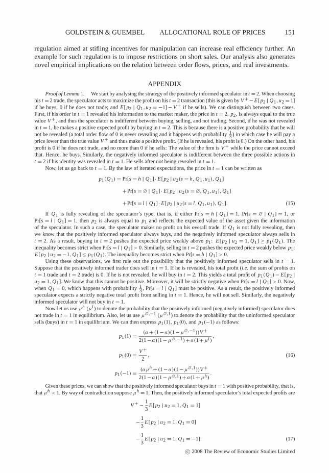
Proof of Lemma 1. We start by analysing the strategy of the positively informed speculator in t = 2. When choosinghis t = 2 trade, the speculator acts to maximize the profit on his t = 2 transaction (this is given by V +− E[p2 | Q1,u2 = 1]if he buys; 0 if he does not trade; and E[p2 | Q1,u2 = −1] − V + if he sells). We can distinguish between two cases.First, if his order in t = 1 revealed his information to the market maker, the price in t = 2, p2, is always equal to the truevalue V +, and thus the speculator is indifferent between buying, selling, and not trading. Second, if he was not revealedin t = 1, he makes a positive expected profit by buying in t = 2. This is because there is a positive probability that he willnot be revealed (a total order flow of 0 is never revealing and it happens with probability 1
3 ) in which case he will pay aprice lower than the true value V + and thus make a positive profit. (If he is revealed, his profit is 0.) On the other hand, hisprofit is 0 if he does not trade, and no more than 0 if he sells: The value of the firm is V + while the price cannot exceedthat. Hence, he buys. Similarly, the negatively informed speculator is indifferent between the three possible actions int = 2 if his identity was revealed in t = 1. He sells after not being revealed in t = 1.
Now, let us go back to t = 1. By the law of iterated expectations, the price in t = 1 can be written as
p1(Q1) = Pr[s = h | Q1] · E[p2 | u2(s = h, Q1,u1), Q1]
+Pr[s =∅ | Q1] · E[p2 | u2(s =∅, Q1,u1), Q1]
+Pr[s = l | Q1] · E[p2 | u2(s = l, Q1,u1), Q1]. (15)
If Q1 is fully revealing of the speculator’s type, that is, if either Pr[s = h | Q1] = 1, Pr[s = ∅ | Q1] = 1, orPr[s = l | Q1] = 1, then p2 is always equal to p1 and reflects the expected value of the asset given the informationof the speculator. In such a case, the speculator makes no profit on his overall trade. If Q1 is not fully revealing, thenwe know that the positively informed speculator always buys, and the negatively informed speculator always sells int = 2. As a result, buying in t = 2 pushes the expected price weakly above p1: E[p2 | u2 = 1, Q1] ≥ p1(Q1). Theinequality becomes strict when Pr[s = l | Q1] > 0. Similarly, selling in t = 2 pushes the expected price weakly below p1:E[p2 | u2 = −1, Q1] ≤ p1(Q1). The inequality becomes strict when Pr[s = h | Q1] > 0.
Using these observations, we first rule out the possibility that the positively informed speculator sells in t = 1.Suppose that the positively informed trader does sell in t = 1. If he is revealed, his total profit (i.e. the sum of profits ont = 1 trade and t = 2 trade) is 0. If he is not revealed, he will buy in t = 2. This yields a total profit of p1(Q1)− E[p2 |u2 = 1, Q1]. We know that this cannot be positive. Moreover, it will be strictly negative when Pr[s = l | Q1] > 0. Now,when Q1 = 0, which happens with probability 1
3 , Pr[s = l | Q1] must be positive. As a result, the positively informedspeculator expects a strictly negative total profit from selling in t = 1. Hence, he will not sell. Similarly, the negativelyinformed speculator will not buy in t = 1.
Now let us use µh (µl ) to denote the probability that the positively informed (negatively informed) speculator doesnot trade in t = 1 in equilibrium. Also, let us use µ∅,−1 (µ∅,1) to denote the probability that the uninformed speculatorsells (buys) in t = 1 in equilibrium. We can then express p1(1), p1(0), and p1(−1) as follows:
p1(1) = (α + (1−α)(1−µ∅,−1))V +2(1−α)(1−µ∅,−1)+α(1+µl )
,
p1(0) = V +2
, (16)
p1(−1) = (αµh + (1−α)(1−µ∅,1))V +2(1−α)(1−µ∅,1)+α(1+µh)
.
Given these prices, we can show that the positively informed speculator buys in t = 1 with positive probability, that is,that µh < 1. By way of contradiction suppose µh = 1. Then, the positively informed speculator’s total expected profits are
V + − 1
3E[p2 | u2 = 1, Q1 = 1]
− 1
3E[p2 | u2 = 1, Q1 = 0]
− 1
3E[p2 | u2 = 1, Q1 = −1]. (17)
c© 2008 The Review of Economic Studies Limited
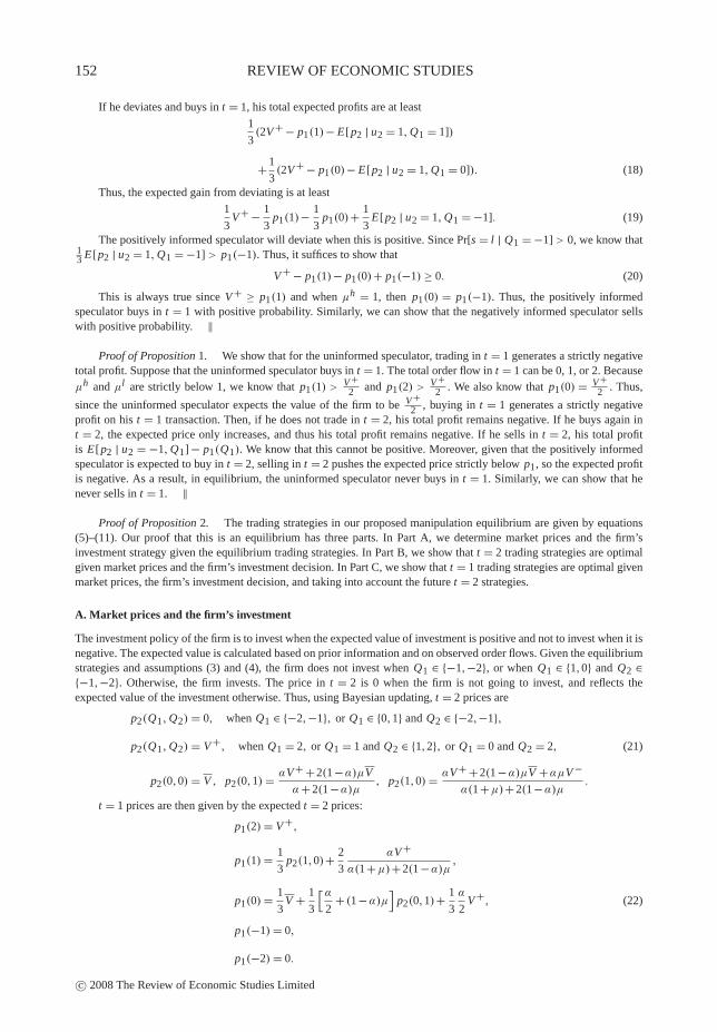
152 REVIEW OF ECONOMIC STUDIES
If he deviates and buys in t = 1, his total expected profits are at least
1
3(2V + − p1(1)− E[p2 | u2 = 1, Q1 = 1])
+ 1
3(2V + − p1(0)− E[p2 | u2 = 1, Q1 = 0]). (18)
Thus, the expected gain from deviating is at least
1
3V + − 1
3p1(1)− 1
3p1(0)+ 1
3E[p2 | u2 = 1, Q1 = −1]. (19)
The positively informed speculator will deviate when this is positive. Since Pr[s = l | Q1 = −1] > 0, we know that13 E[p2 | u2 = 1, Q1 = −1] > p1(−1). Thus, it suffices to show that
V + − p1(1)− p1(0)+ p1(−1) ≥ 0. (20)
This is always true since V + ≥ p1(1) and when µh = 1, then p1(0) = p1(−1). Thus, the positively informedspeculator buys in t = 1 with positive probability. Similarly, we can show that the negatively informed speculator sellswith positive probability. ‖
Proof of Proposition 1. We show that for the uninformed speculator, trading in t = 1 generates a strictly negativetotal profit. Suppose that the uninformed speculator buys in t = 1. The total order flow in t = 1 can be 0, 1, or 2. Becauseµh and µl are strictly below 1, we know that p1(1) > V +
2 and p1(2) > V +2 . We also know that p1(0) = V +
2 . Thus,
since the uninformed speculator expects the value of the firm to be V +2 , buying in t = 1 generates a strictly negative
profit on his t = 1 transaction. Then, if he does not trade in t = 2, his total profit remains negative. If he buys again int = 2, the expected price only increases, and thus his total profit remains negative. If he sells in t = 2, his total profitis E[p2 | u2 = −1, Q1] − p1(Q1). We know that this cannot be positive. Moreover, given that the positively informedspeculator is expected to buy in t = 2, selling in t = 2 pushes the expected price strictly below p1, so the expected profitis negative. As a result, in equilibrium, the uninformed speculator never buys in t = 1. Similarly, we can show that henever sells in t = 1. ‖
Proof of Proposition 2. The trading strategies in our proposed manipulation equilibrium are given by equations(5)–(11). Our proof that this is an equilibrium has three parts. In Part A, we determine market prices and the firm’sinvestment strategy given the equilibrium trading strategies. In Part B, we show that t = 2 trading strategies are optimalgiven market prices and the firm’s investment decision. In Part C, we show that t = 1 trading strategies are optimal givenmarket prices, the firm’s investment decision, and taking into account the future t = 2 strategies.
A. Market prices and the firm’s investment
The investment policy of the firm is to invest when the expected value of investment is positive and not to invest when it isnegative. The expected value is calculated based on prior information and on observed order flows. Given the equilibriumstrategies and assumptions (3) and (4), the firm does not invest when Q1 ∈ {−1,−2}, or when Q1 ∈ {1,0} and Q2 ∈{−1,−2}. Otherwise, the firm invests. The price in t = 2 is 0 when the firm is not going to invest, and reflects theexpected value of the investment otherwise. Thus, using Bayesian updating, t = 2 prices are
p2(Q1, Q2) = 0, when Q1 ∈ {−2,−1}, or Q1 ∈ {0,1} and Q2 ∈ {−2,−1},
p2(Q1, Q2) = V +, when Q1 = 2, or Q1 = 1 and Q2 ∈ {1,2}, or Q1 = 0 and Q2 = 2, (21)
p2(0,0) = V , p2(0,1) = αV + +2(1−α)µV
α +2(1−α)µ, p2(1,0) = αV + +2(1−α)µV +αµV −
α(1+µ)+2(1−α)µ.
t = 1 prices are then given by the expected t = 2 prices:
p1(2) = V +,
p1(1) = 1
3p2(1,0)+ 2
3
αV +α(1+µ)+2(1−α)µ
,
p1(0) = 1
3V + 1
3
[α
2+ (1−α)µ
]p2(0,1)+ 1
3
α
2V +, (22)
p1(−1) = 0,
p1(−2) = 0.
c© 2008 The Review of Economic Studies Limited
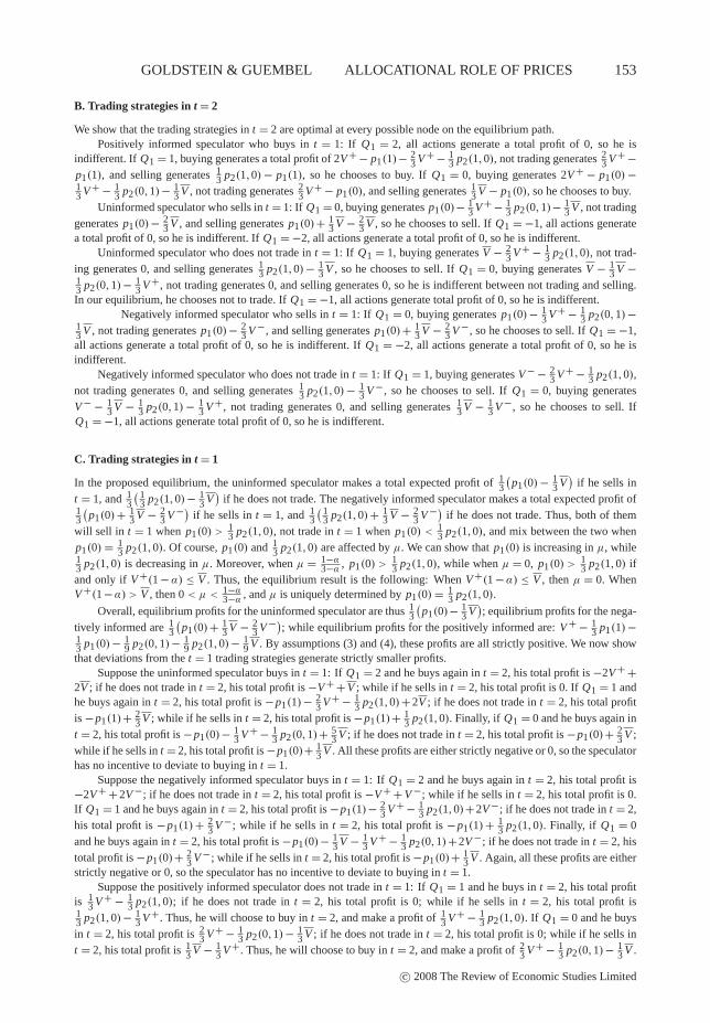
GOLDSTEIN & GUEMBEL ALLOCATIONAL ROLE OF PRICES 153
B. Trading strategies in t = 2
We show that the trading strategies in t = 2 are optimal at every possible node on the equilibrium path.Positively informed speculator who buys in t = 1: If Q1 = 2, all actions generate a total profit of 0, so he is
indifferent. If Q1 = 1, buying generates a total profit of 2V + − p1(1)− 23 V + − 1
3 p2(1,0), not trading generates 23 V + −
p1(1), and selling generates 13 p2(1,0) − p1(1), so he chooses to buy. If Q1 = 0, buying generates 2V + − p1(0) −
13 V + − 1
3 p2(0,1)− 13 V , not trading generates 2
3 V + − p1(0), and selling generates 13 V − p1(0), so he chooses to buy.
Uninformed speculator who sells in t = 1: If Q1 = 0, buying generates p1(0)− 13 V + − 1
3 p2(0,1)− 13 V , not trading
generates p1(0)− 23 V , and selling generates p1(0)+ 1
3 V − 23 V , so he chooses to sell. If Q1 = −1, all actions generate
a total profit of 0, so he is indifferent. If Q1 = −2, all actions generate a total profit of 0, so he is indifferent.Uninformed speculator who does not trade in t = 1: If Q1 = 1, buying generates V − 2
3 V + − 13 p2(1,0), not trad-
ing generates 0, and selling generates 13 p2(1,0)− 1
3 V , so he chooses to sell. If Q1 = 0, buying generates V − 13 V −
13 p2(0,1)− 1
3 V +, not trading generates 0, and selling generates 0, so he is indifferent between not trading and selling.In our equilibrium, he chooses not to trade. If Q1 = −1, all actions generate total profit of 0, so he is indifferent.
Negatively informed speculator who sells in t = 1: If Q1 = 0, buying generates p1(0)− 13 V + − 1
3 p2(0,1)−13 V , not trading generates p1(0)− 2
3 V −, and selling generates p1(0)+ 13 V − 2
3 V −, so he chooses to sell. If Q1 = −1,all actions generate a total profit of 0, so he is indifferent. If Q1 = −2, all actions generate a total profit of 0, so he isindifferent.
Negatively informed speculator who does not trade in t = 1: If Q1 = 1, buying generates V − − 23 V + − 1
3 p2(1,0),not trading generates 0, and selling generates 1
3 p2(1,0) − 13 V −, so he chooses to sell. If Q1 = 0, buying generates
V − − 13 V − 1
3 p2(0,1) − 13 V +, not trading generates 0, and selling generates 1
3 V − 13 V −, so he chooses to sell. If
Q1 = −1, all actions generate total profit of 0, so he is indifferent.
C. Trading strategies in t = 1
In the proposed equilibrium, the uninformed speculator makes a total expected profit of 13
(p1(0) − 1
3 V)
if he sells int = 1, and 1
3
( 13 p2(1,0)− 1
3 V)
if he does not trade. The negatively informed speculator makes a total expected profit of13
(p1(0)+ 1
3 V − 23 V −)
if he sells in t = 1, and 13
( 13 p2(1,0)+ 1
3 V − 23 V −)
if he does not trade. Thus, both of themwill sell in t = 1 when p1(0) > 1
3 p2(1,0), not trade in t = 1 when p1(0) < 13 p2(1,0), and mix between the two when
p1(0) = 13 p2(1,0). Of course, p1(0) and 1
3 p2(1,0) are affected by µ. We can show that p1(0) is increasing in µ, while13 p2(1,0) is decreasing in µ. Moreover, when µ = 1−α
3−α , p1(0) > 13 p2(1,0), while when µ = 0, p1(0) > 1
3 p2(1,0) ifand only if V +(1 −α) ≤ V . Thus, the equilibrium result is the following: When V +(1 −α) ≤ V , then µ = 0. WhenV +(1−α) > V , then 0 < µ < 1−α
3−α , and µ is uniquely determined by p1(0) = 13 p2(1,0).
Overall, equilibrium profits for the uninformed speculator are thus 13
(p1(0)− 1
3 V); equilibrium profits for the nega-
tively informed are 13
(p1(0)+ 1
3 V − 23 V −)
; while equilibrium profits for the positively informed are: V + − 13 p1(1)−
13 p1(0)− 1
9 p2(0,1)− 19 p2(1,0)− 1
9 V . By assumptions (3) and (4), these profits are all strictly positive. We now showthat deviations from the t = 1 trading strategies generate strictly smaller profits.
Suppose the uninformed speculator buys in t = 1: If Q1 = 2 and he buys again in t = 2, his total profit is −2V + +2V ; if he does not trade in t = 2, his total profit is −V + + V ; while if he sells in t = 2, his total profit is 0. If Q1 = 1 andhe buys again in t = 2, his total profit is −p1(1)− 2
3 V + − 13 p2(1,0)+ 2V ; if he does not trade in t = 2, his total profit
is −p1(1)+ 23 V ; while if he sells in t = 2, his total profit is −p1(1)+ 1
3 p2(1,0). Finally, if Q1 = 0 and he buys again int = 2, his total profit is −p1(0)− 1
3 V + − 13 p2(0,1)+ 5
3 V ; if he does not trade in t = 2, his total profit is −p1(0)+ 23 V ;
while if he sells in t = 2, his total profit is −p1(0)+ 13 V . All these profits are either strictly negative or 0, so the speculator
has no incentive to deviate to buying in t = 1.Suppose the negatively informed speculator buys in t = 1: If Q1 = 2 and he buys again in t = 2, his total profit is
−2V + +2V −; if he does not trade in t = 2, his total profit is −V + + V −; while if he sells in t = 2, his total profit is 0.If Q1 = 1 and he buys again in t = 2, his total profit is −p1(1)− 2
3 V + − 13 p2(1,0)+2V −; if he does not trade in t = 2,
his total profit is −p1(1)+ 23 V −; while if he sells in t = 2, his total profit is −p1(1)+ 1
3 p2(1,0). Finally, if Q1 = 0and he buys again in t = 2, his total profit is −p1(0)− 1
3 V − 13 V + − 1
3 p2(0,1)+2V −; if he does not trade in t = 2, histotal profit is −p1(0)+ 2
3 V −; while if he sells in t = 2, his total profit is −p1(0)+ 13 V . Again, all these profits are either
strictly negative or 0, so the speculator has no incentive to deviate to buying in t = 1.Suppose the positively informed speculator does not trade in t = 1: If Q1 = 1 and he buys in t = 2, his total profit
is 13 V + − 1
3 p2(1,0); if he does not trade in t = 2, his total profit is 0; while if he sells in t = 2, his total profit is13 p2(1,0)− 1
3 V +. Thus, he will choose to buy in t = 2, and make a profit of 13 V + − 1
3 p2(1,0). If Q1 = 0 and he buysin t = 2, his total profit is 2
3 V + − 13 p2(0,1)− 1
3 V ; if he does not trade in t = 2, his total profit is 0; while if he sells int = 2, his total profit is 1
3 V − 13 V +. Thus, he will choose to buy in t = 2, and make a profit of 2
3 V + − 13 p2(0,1)− 1
3 V .
c© 2008 The Review of Economic Studies Limited
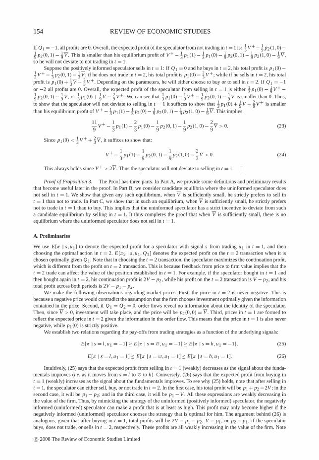
154 REVIEW OF ECONOMIC STUDIES
If Q1 = −1, all profits are 0. Overall, the expected profit of the speculator from not trading in t = 1 is: 13 V +− 1
9 p2(1,0)−19 p2(0,1)− 1
9 V . This is smaller than his equilibrium profit of V + − 13 p1(1)− 1
3 p1(0)− 19 p2(0,1)− 1
9 p2(1,0)− 19 V ,
so he will not deviate to not trading in t = 1.Suppose the positively informed speculator sells in t = 1: If Q1 = 0 and he buys in t = 2, his total profit is p1(0)−
13 V + − 1
3 p2(0,1)− 13 V ; if he does not trade in t = 2, his total profit is p1(0)− 2
3 V +; while if he sells in t = 2, his totalprofit is p1(0)+ 1
3 V − 23 V +. Depending on the parameters, he will either choose to buy or to sell in t = 2. If Q1 = −1
or −2 all profits are 0. Overall, the expected profit of the speculator from selling in t = 1 is either 13 p1(0) − 1
9 V + −19 p2(0,1)− 1
9 V , or 13 p1(0)+ 1
9 V − 29 V +. We can see that 1
3 p1(0)− 19 V + − 1
9 p2(0,1)− 19 V is smaller than 0. Thus,
to show that the speculator will not deviate to selling in t = 1 it suffices to show that 13 p1(0)+ 1
9 V − 29 V + is smaller
than his equilibrium profit of V + − 13 p1(1)− 1
3 p1(0)− 19 p2(0,1)− 1
9 p2(1,0)− 19 V . This implies
11
9V + − 1
3p1(1)− 2
3p1(0)− 1
9p2(0,1)− 1
9p2(1,0)− 2
9V > 0. (23)
Since p1(0) < 13 V + + 2
3 V , it suffices to show that:
V + − 1
3p1(1)− 1
9p2(0,1)− 1
9p2(1,0)− 2
3V > 0. (24)
This always holds since V + > 2V . Thus the speculator will not deviate to selling in t = 1. ‖
Proof of Proposition 3. The Proof has three parts. In Part A, we provide some definitions and preliminary resultsthat become useful later in the proof. In Part B, we consider candidate equilibria where the uninformed speculator doesnot sell in t = 1. We show that given any such equilibrium, when V is sufficiently small, he strictly prefers to sell int = 1 than not to trade. In Part C, we show that in such an equilibrium, when V is sufficiently small, he strictly prefersnot to trade in t = 1 than to buy. This implies that the uninformed speculator has a strict incentive to deviate from sucha candidate equilibrium by selling in t = 1. It thus completes the proof that when V is sufficiently small, there is noequilibrium where the uninformed speculator does not sell in t = 1.
A. Preliminaries
We use E[π | s,u1] to denote the expected profit for a speculator with signal s from trading u1 in t = 1, and thenchoosing the optimal action in t = 2. E[π2 | s,u1, Q1] denotes the expected profit on the t = 2 transaction when it ischosen optimally given Q1. Note that in choosing the t = 2 transaction, the speculator maximizes the continuation profit,which is different from the profit on t = 2 transaction. This is because feedback from price to firm value implies that thet = 2 trade can affect the value of the position established in t = 1. For example, if the speculator bought in t = 1 andthen bought again in t = 2, his continuation profit is 2V − p2, while his profit on the t = 2 transaction is V − p2, and histotal profit across both periods is 2V − p1 − p2.
We make the following observations regarding market prices. First, the price in t = 2 is never negative. This isbecause a negative price would contradict the assumption that the firm chooses investment optimally given the informationcontained in the price. Second, if Q1 = Q2 = 0, order flows reveal no information about the identity of the speculator.Then, since V > 0, investment will take place, and the price will be p2(0,0) = V . Third, prices in t = 1 are formed toreflect the expected price in t = 2 given the information in the order flow. This means that the price in t = 1 is also nevernegative, while p1(0) is strictly positive.
We establish two relations regarding the pay-offs from trading strategies as a function of the underlying signals:
E[π | s = l,u1 = −1] ≥ E[π | s =∅,u1 = −1] ≥ E[π | s = h,u1 = −1], (25)
E[π | s = l,u1 = 1] ≤ E[π | s =∅,u1 = 1] ≤ E[π | s = h,u1 = 1]. (26)
Intuitively, (25) says that the expected profit from selling in t = 1 (weakly) decreases as the signal about the funda-mentals improves (i.e. as it moves from s = l to ∅ to h). Conversely, (26) says that the expected profit from buying int = 1 (weakly) increases as the signal about the fundamentals improves. To see why (25) holds, note that after selling int = 1, the speculator can either sell, buy, or not trade in t = 2. In the first case, his total profit will be p1 + p2 −2V ; in thesecond case, it will be p1 − p2; and in the third case, it will be p1 − V . All these expressions are weakly decreasing inthe value of the firm. Thus, by mimicking the strategy of the uninformed (positively informed) speculator, the negativelyinformed (uninformed) speculator can make a profit that is at least as high. This profit may only become higher if thenegatively informed (uninformed) speculator chooses the strategy that is optimal for him. The argument behind (26) isanalogous, given that after buying in t = 1, total profits will be 2V − p1 − p2, V − p1, or p2 − p1, if the speculatorbuys, does not trade, or sells in t = 2, respectively. These profits are all weakly increasing in the value of the firm. Note
c© 2008 The Review of Economic Studies Limited
GOLDSTEIN & GUEMBEL ALLOCATIONAL ROLE OF PRICES 155
that the inequality becomes strict if the speculator strictly prefers to buy in t = 2 and if investment happens with positiveprobability afterwards. In Lemma 3, we show that the positively informed speculator strictly prefers to buy in t = 2 afterbuying in t = 1. This generates investment with positive probability since investment always happens after Q1 = Q2 = 0.Thus, we get that the following strict inequality holds:
E[π | s =∅,u1 = 1] < E[π | s = h,u1 = 1]. (27)
Finally, we conclude this part of the proof by stating three lemmas that characterize the behaviour of speculators ina candidate equilibrium, where the uninformed speculator does not sell in t = 1. The proofs of these lemmas appear afterthe proof of Proposition 3.
Lemma 2. In any candidate equilibrium, where the uninformed speculator does not sell in t = 1, and V is suffi-ciently small, the following holds:
(1) The negatively informed speculator does not buy in t = 1.(2) When p1 > 0, the negatively informed speculator does not buy in t = 2.(3) After Q1 = 0, the negatively informed speculator always sells in t = 2.
Lemma 3. In any candidate equilibrium, where off-the-path beliefs satisfy the intuitive criterion, the uninformedspeculator does not sell in t = 1, and V is sufficiently small, the following holds:
(1) The positively informed speculator buys in t = 2 after an order flow of Q1 if (a) V + > p1(Q1) > 0, (b) u1 ∈ {0,1}and (c) investment occurs following Q2 = 0.
(2) The positively informed speculator does not sell in t = 1.(3) After Q1 = 0 or 1, the positively informed speculator always buys in t = 2. After Q1 = 2, the positively informed
speculator always buys in t = 2, as long as the uninformed speculator buys in t = 1 in equilibrium.
Lemma 4. In a candidate equilibrium, where the uninformed speculator does not sell in t = 1, and V is sufficientlysmall, the uninformed speculator does not buy in t = 2 after Q1 = 0.
B. Not trading vs. selling
The expected profit of the uninformed speculator from not trading in t = 1 is E[π | s =∅,u1 = 0], which can be writtenas
1
3E[π2 | s =∅,u1 = 0, Q1 = −1]
+ 1
3E[π2 | s =∅,u1 = 0, Q1 = 0]
+ 1
3E[π2 | s =∅,u1 = 0, Q1 = 1] . (28)
If he sells, he gets at least 13 (p1(−2)+ p1(−1)+ p1(0))− V on his t = 1 transaction, and then
1
3E[π2 | s =∅,u1 = −1, Q1 = −1]
+ 1
3E[π2 | s =∅,u1 = −1, Q1 = 0]
+ 1
3E[π2 | s =∅,u1 = −1, Q1 = −2] , (29)
on his t = 2 transaction. If he sells and Q1 = −1 or 0, the profit he can make on his t = 2 transaction is at least as high asthe profit he makes after he does not trade and Q1 = −1 or 0. If he sells and Q1 = −2, he makes at least 0 on his t = 2transaction. Thus, he strictly prefers u1 = −1 to u1 = 0 when
1
3(p1(−2)+ p1(−1)+ p1(0))− V >
1
3E[π2 | s =∅,u1 = 0, Q1 = 1]. (30)
Given that prices are never negative, and taking a sufficiently small V , it is sufficient to show that
E[π2 | s =∅,u1 = 0, Q1 = 1] < p1(0). (31)
c© 2008 The Review of Economic Studies Limited
156 REVIEW OF ECONOMIC STUDIES
We now characterize p1(0). In equilibrium, Q1 = 0 can be generated by the positively informed, negatively in-formed, and uninformed speculator, with probabilities α
2 , α2 , and (1 − α), respectively. From Lemma 2 we know that
after Q1 = 0, the negatively informed speculator always sells in t = 2. From Lemma 3 we know that after Q1 = 0, thepositively informed speculator always buys in t = 2. From Lemma 4 we know that after Q1 = 0, the uninformed specu-lator never buys in t = 2. We use ξ to denote the probability that the uninformed speculator does not trade in t = 2 afterQ1 = 0. Using these results, we can characterize t = 2 prices, conditional on Q1 = 0. With probability 1
3α2 , Q2 = 2,
and the price p2(0,2) is given by V +. With probability 13
α2 + 1
3 (1 −α)ξ , Q2 = 1, and the price p2(0,1) is given by13
α2 V ++ 1
3 (1−α)ξV13
α2 + 1
3 (1−α)ξ. With probability 1
3 , Q2 = 0, and the price p2(0,0) is given by V . With probability 13
α2 + 1
3 (1−α),
Q2 = −1, and the price p2(0,−1) is given by 0 (because the order flow can be generated by the uninformed speculatoror by the negatively informed speculator, and thus, for a sufficiently small V , the investment is rejected). With probability13
α2 + 1
3 (1−α)(1−ξ), Q2 = −2, and the price p2(0,−2) is given by 0. p1(0) is then a weighted average of the possiblet = 2 prices. It is given by
α
3V + + 1
3((1−α)ξ +1)V . (32)
Thus, to prove (31), it is sufficient to show that
E[π2 | s =∅,u1 = 0, Q1 = 1] <α
3V +. (33)
Now, let us characterize E[π2 | s = ∅,u1 = 0, Q1 = 1]. If the uninformed speculator does not trade in t = 2, hisprofit is 0. If he buys, he makes a maximum profit of V . Both these profits are clearly below α
3 V +. If he sells in t = 2 hismaximum profit is 1
3 (p2(1,−2)+ p2(1,−1)+ p2(1,0)). Thus, to prove (33), it is sufficient to show that
p2(1,−2)+ p2(1,−1)+ p2(1,0) < αV +. (34)
From Lemma 3 we know that after Q1 = 1, the positively informed speculator always buys in t = 2. Thus, whenQ2 = −2 or −1, it is known that the positively informed speculator is not behind the trade. As a result, p2(1,−2) andp2(1,−1) are at most V . Given that the uninformed speculator does not sell in t = 1, the maximum value of p2(1,0) isαV ++2(1−α)V
2−α . Thus, a sufficient condition for (34) is
α
2−αV + + 6−4α
2−αV < αV +. (35)
Since α < 1, this always holds for a sufficiently small V .
C. Not trading vs. buying
The expected profit of the uninformed trader from not trading in t = 1 is given by (28). If he buys, he gets at mostV − 1
3 (p1(0)+ p1(1)+ p1(2)) on his t = 1 transaction, and then
1
3E[π2 | s =∅,u1 = 1, Q1 = 0]
+ 1
3E[π2 | s =∅,u1 = 1, Q1 = 1]
+ 1
3E[π2 | s =∅,u1 = 1, Q1 = 2] , (36)
on his t = 2 transaction. If he does not trade and Q1 = 1 or 0, the profit he can make on his t = 2 transaction is at least ashigh as the profit he makes after he buys and Q1 = 1 or 0. If he does not trade and Q1 = −1, he makes at least 0 on hist = 2 transaction. Thus, he strictly prefers u1 = 0 to u1 = 1 when
V − 1
3(p1(0)+ p1(1)+ p1(2))+ 1
3E[π2 | s =∅,u1 = 1, Q1 = 2] < 0. (37)
Given (32) and given that prices cannot be negative, for a sufficiently small V , it is sufficient to show that
E[π2 | s =∅,u1 = 1, Q1 = 2]− p1(2) <α
3V +. (38)
If the uninformed speculator does not trade in t = 2 after Q1 = 2, his t = 2 profit is 0, and the inequality clearlyholds. If the uninformed speculator buys in t = 2 after Q1 = 2, his t = 2 profit cannot exceed V , and the inequality
c© 2008 The Review of Economic Studies Limited
GOLDSTEIN & GUEMBEL ALLOCATIONAL ROLE OF PRICES 157
holds for a sufficiently small V . The more interesting case is when the uninformed speculator sells in t = 2 after Q1 = 2.In this case, his t = 2 profit is at most 1
3 (p2(2,0)+ p2(2,−1)+ p2(2,−2)). Thus, we need to show that
1
3(p2(2,0)+ p2(2,−1)+ p2(2,−2))− p1(2) <
α
3V +. (39)
From Lemma 2 we know that the negatively informed speculator does not buy in t = 1. Thus, if the uninformedspeculator buys in t = 1 in equilibrium, Q1 = 2 can result from both the positively informed and the uninformed specu-lator. Then, from Lemma 3, the positively informed speculator buys in t = 2. Thus, given that p1 is a weighted averageof possible t = 2 prices, selling in t = 2 will push the price down, implying that the L.H.S. of (39) is at most 0, and thusthat (39) holds. ‖
Proof of Lemma 2.Part 1: By way of contradiction, suppose that the negatively informed speculator buys in t = 1. In that period,
total order flow will be 0, 1, or 2. Since prices are either 0 or positive, and the value of the firm, conditional on s = l, iseither 0 (if the firm does not invest) or negative (if the firm invests), he maximizes his expected profit by selling in t = 2.As a result, the maximum total profit from buying in t = 1 is
1
3(E[p2 | Q1 = 0,u2 = −1]− p1(0))
+ 1
3(E[p2 | Q1 = 1,u2 = −1]− p1(1))
+ 1
3(E[p2 | Q1 = 2,u2 = −1]− p1(2)). (40)
If, instead, the speculator deviates to not trading in t = 1 and selling in t = 2, his expected profit is
1
3(E[p2 | Q1 = 0,u2 = −1]− E[V | s = l, Q1 = 0,u2 = −1])
+ 1
3(E[p2 | Q1 = 1,u2 = −1]− E[V | s = l, Q1 = 1,u2 = −1])
+ 1
3(E[p2 | Q1 = −1,u2 = −1]− E[V | s = l, Q1 = −1,u2 = −1]). (41)
We know that prices are always 0 or positive, and firm value conditional on s = l is either 0 or negative. We alsoknow that p1(0) is strictly positive and that investment happens after Q1 = Q2 = 0, generating a negative value of V −.Thus, the sum of the first two rows in (40) is strictly smaller than the sum of the first two rows in (41). Also, the lastrow in (41) is at least 0. Thus, to show that the negatively informed speculator would deviate from buying in t = 1 to nottrading, we need to show that the last row in (40) is at most 0. That is, the profit from buying in t = 1 and then sellingafter Q1 = 2 cannot be strictly positive. Here, we need to distinguish between two cases. First, if, following Q1 = 2, thenegatively informed speculator sells with probability 1, the expected price in equilibrium following a sell order cannotincrease. Second, if, following Q1 = 2, he sells with probability less than 1, it means he is indifferent between sellingand either buying or not trading. Since we already know that, conditional on s = l, buying or not trading cannot generatea strictly positive continuation profit, his continuation profit, and thus his total profit, cannot be strictly positive.
Part 2: From Part 1 we know that the negatively informed speculator did not buy in t = 1. Suppose that he did nottrade in t = 1. Then, his continuation profit from buying is E[V − p2 | s = l,u2 = 1] ≤ 0, with strict inequality when thefirm invests after some Q2 ∈ {0,1,2}. Alternatively, the continuation profit from selling is E[p2 −V | s = l,u2 = −1] ≥ 0,with strict inequality if the firm invests following some Q2 ∈ {−2,−1,0}. Hence, as long as investment happens aftersome Q2 (i.e. as long as p1 > 0), selling in t = 2 is strictly preferred over buying. Now, suppose that the negativelyinformed speculator sold in t = 1. His continuation profit from buying is −E[p2 | u2 = 1] ≤ 0, with strict inequalitywhen the firm invests after some Q2 ∈ {0,1,2}. Alternatively, the continuation profit from selling is E[p2 − 2V | s = l,u2 = −1] ≥ 0, with strict inequality if the firm invests following some Q2 ∈ {−2,−1,0}. Hence, as before, as longinvestment happens after some Q2, selling in t = 2 is strictly preferred over buying.
Part 3: Since p1(0) > 0, we know from Part 2 that the negatively informed speculator does not buy in t = 2 afterQ1 = 0. We now show that he strictly prefers to sell in t = 2 than not to trade. Suppose that he did not trade in t = 1. Then,his continuation profit from selling is E[p2 − V | s = l,u2 = −1], while his continuation profit from not trading is 0. Thecontinuation profit from selling is strictly greater since investment happens after Q2 = 0 generating a positive price anda negative value. Now, suppose that the negatively informed speculator sold in t = 1. His continuation profit from sellingis E[p2 −2V | s = l,u2 = −1], while his continuation profit from not trading is −E[V | s = l,u2 = 0]. After comparing
c© 2008 The Review of Economic Studies Limited
158 REVIEW OF ECONOMIC STUDIES
these expressions, we find that the continuation profit from selling is strictly greater given that investment happens afterQ2 = 0 generating a positive price and a negative value of V −. ‖
Proof of Lemma 3.Part 1: A first step for the proof of this lemma is to show that if investment occurs after any t = 2 order flow
that is consistent with u2 = −1 (i.e. Q2 ∈ {−2,−1,0}), it also occurs for all order flows consistent with u2 = 1(i.e. Q2 ∈ {0,1,2}).
To see this note that when investment occurs after some order flow consistent with u2 = −1, the negatively informedspeculator has a strict incentive to sell in t = 2. If he has a short position (no position), selling generates a continuationprofit of E[p2 −2V | s = l,u2 = −1] (E[p2 −V | s = l,u2 = −1]), whereas not trading generates a continuation profit ofE[−V | s = l,u2 = 0] (0). The continuation profit from selling is strictly greater given that investment sometimes occursafter he sells, generating a positive price and a negative value of V −. Then, given that the negatively informed speculatoralways sells, an order flow of 1 or 2 cannot be generated by the negatively informed speculator. Investment must thereforealways occur after such order flows. (This is unless Q2 ∈ {1,2} is off the equilibrium path and the market maker and themanager attach a sufficiently high probability to the deviation being due to the negatively informed speculator. Such abelief, however, violates the intuitive criterion since the negatively informed speculator strictly prefers to sell regardless ofhis t = 1 position and the off-the-path beliefs, while there exist off-the-path beliefs under which the positively informedspeculator would be better off from deviating to buying.) The probability that an order flow of 0 is generated by thenegatively informed speculator is not higher than the probability that an order flow of −2 or −1 was generated by him.Thus, if investment happens after an order flow of −2 or −1, it must happen after an order flow of 0.
Based on this, we can now prove that the positively informed speculator strictly prefers to buy in t = 2 after heacquired a long position in t = 1, and p1 was different from 0 or V +. Buying in t = 2 yields a continuation profit ofE[2V − p2 | s = h,u2 = 1]; not trading yields a continuation profit of E[V | s = h,u2 = 0]; and selling yields a con-tinuation profit of E[p2 | u2 = −1]. Thus, buying is strictly better than selling if 2E[V | s = h,u2 = 1]− E[p2 | u2 = 1]−E[p2 | u2 = −1] > 0 . If investment happens after any Q2 ∈ {−2,−1,0}, it must happen after all Q2 ∈ {0,1,2}. Thus,E[V | s = h,u2 = 1] = V +, while both E[p2 | u2 = 1] and E[p2 | u2 = −1] must be smaller than V +, since p1 waslower than V +, so p2(Q2 = 0) must also be below V +. Thus, the above expression is positive. If investment neverhappens after u2 = −1, it must happen sometime after u2 = 1 (since p1 was higher than 0). Then, E[p2 | u2 = −1] = 0,while E[V | s = h,u2 = 1] > 0, so the above expression is positive. Similarly, buying is preferable to not trading if2E[V | s = h,u2 = 1]− E[p2 | u2 = 1]− E[V | s = h,u2 = 0] > 0. Using similar arguments and the fact that investmentalways happens after Q2 = 2 (since the negatively informed speculator does not buy in t = 2) we can show that thisindeed holds.
Now, let us analyse the choice of the positively informed trader in t = 2 after he did not trade in t = 1, and 0< p1 < V +. Buying in t = 2 yields a continuation profit of E[V − p2 | s = h,u2 = 1]; not trading yields a continua-tion profit of 0; and selling yields a continuation profit of E[p2 − V | s = h,u2 = −1]. Using the above arguments, weknow that buying is strictly better than selling and not trading if investment happens at some Q2 consistent with u2 = −1(for example, Q2 = 0).
Part 2: We show that there cannot be an equilibrium, in which the positively informed speculator sells in t = 1and the uninformed speculator does not. Suppose the positively informed speculator sells in t = 1. This implies thatE[π | s = h,u1 = −1] ≥ E[π | s = h,u1 = 1]. Then, by (25), (26), and (27), the uninformed speculator strictly prefersselling to buying in t = 1. We now show that in such an equilibrium, the uninformed speculator would strictly preferto sell than not to trade in t = 1. The maximum total profit for the positively informed speculator from u1 = −1 is13 (p1(0) + p1(−1) + p1(−2)). If instead u1 = 0, he can buy in t = 2, and, since investment always happens afterQ1 = Q2 = 0 (with a price of V ), guarantee an expected profit of at least 1
9 (V + − V ). Since the positively informedspeculator sells in t = 1, we know that
p1(0)+ p1(−1)+ p1(−2) ≥ 1
3(V + − V ). (42)
If the uninformed speculator does not trade in t = 1, Q1 will be −1, 0, or 1. For each one of these realizations, hemakes some profit π2 on his t = 2 transaction. If the uninformed speculator sells in t = 1, Q1 will be −2, −1, or 0. Thus,by selling in t = 1, he can replicate the t = 2 profit he makes after not trading when Q1 is either −1, or 0. In addition, hegets the profit on his t = 1 transaction, which is at least 1
3 (p1(0)+ p1(−1)+ p1(−2))− V . As a result, his profit fromselling in t = 1 is strictly greater than his profit from not trading if
p1(0)+ p1(−1)+ p1(−2) > 3V + E[π2 | s =∅,u1 = 0, Q1 = 1]. (43)
Given (42), for a sufficiently small V , it is sufficient to show that
E[π2 | s =∅,u1 = 0, Q1 = 1] <1
3V +. (44)
c© 2008 The Review of Economic Studies Limited
GOLDSTEIN & GUEMBEL ALLOCATIONAL ROLE OF PRICES 159
If the uninformed speculator does not trade in t = 2, his total profit his 0, which is clearly below 13 V +. If he buys,
he pays a price, and gets an asset with a maximum value of V (conditional on his information), so for a sufficiently smallV , his profit is below 1
3 V +. If the uninformed speculator sells in t = 2 his maximum expected profit is 13 (p2(1,0)+
p2(1,−1)+ p2(1,−2)). Note that Q1 = 1 is consistent with a positively informed speculator who either bought or didnot trade in t = 1. We know that the positively informed speculator always buys in t = 2 after buying in t = 1. If he didnot trade in t = 1, we need to distinguish between the case in which he strictly prefers to buy in t = 2 and the case inwhich he does not. In the second case, we know from Part 1 of this lemma that investment does not happen after any Q2consistent with u2 = −1. Thus, p2(1,0) = p2(1,−1) = p2(1,−2) = 0, and the uninformed speculator makes no profitfrom selling in t = 2. If the positively informed speculator strictly prefers to buy in t = 2, both p2(1,−1) and p2(1,−2)
cannot be greater than V , as Q2 = −1 and Q2 = −2 are inconsistent with the positively informed speculator. Moreover,p2(1,0) has to be below V +, since Q1 = 1 and Q2 = 0 is consistent with the uninformed speculator when he does notsell in t = 1. Thus, 1
3 (p2(1,0)+ p2(1,−1)+ p2(1,−2)) < 13 (V + + 2V ). This implies that, for a sufficiently small V ,
(44) holds.Part 3: This follows directly from the first two parts of the lemma and the fact (which follows from the investment
strategies proven above) that after Q1 ∈ {0,1,2} and Q2 = 0 the firm invests. ‖
Proof of Lemma 4. Given that the speculator is uninformed, the value of the firm is either V or 0. Thus, fora sufficiently small V , the uninformed speculator chooses his t = 2 transaction to maximize the t = 2 profit (i.e. theeffect of the transaction on the value of his existing position is negligible). We know from Lemmas 2 and 3 that thenegatively informed speculator always sells and the positively informed speculator always buys after Q1 = 0. Thus, ifthe uninformed speculator buys after Q1 = 0, the price he pays at Q2 = 1 and Q2 = 2 is a weighted average between Vand V +. Since the value of the asset, given his information, does not exceed V , he makes a loss on his t = 2 transaction.Thus, he prefers not to buy. ‖
Proof of Proposition 4. Suppose that the uninformed speculator buys in t = 1. Since prices are either 0 or positive,and the expected value of the firm, conditional on s = ∅ and V < 0 is either 0 (if the firm does not invest) or negative(if the firm invests), he cannot make a strictly positive profit unless he sells in t = 2. Selling in t = 2 generates a totalprofit of
1
3(E[p2 | Q1 = 0,u2 = −1]− p1(0))+ 1
3(E[p2 | Q1 = 1,u2 = −1]− p1(1))
+ 1
3(E[p2 | Q1 = 2,u2 = −1]− p1(2)). (45)
First, note that the third term of (45) cannot be strictly positive. If it is strictly positive, then E[p2 | Q1 = 2,
u2 = −1] > 0. Given that V < 0 and that at Q1 = 2 the speculator has a long position, this implies that the uninformedspeculator and the negatively informed speculator strictly prefer to sell in t = 2. As a result, selling pushes the priceweakly below p1(2), and so E[p2 | Q1 = 2,u2 = −1]− p1(2) ≤ 0.
Now, for the uninformed speculator to make a positive profit, either E[p2 | Q1 = 0,u2 = −1] − p1(0) > 0 orE[p2 | Q1 = 1,u2 = −1] − p1(1) > 0, or both, must hold. This implies that investment happens after some nodesfollowing Q1 = 0 and/or Q1 = 1, and thus p1(0) and/or p1(1) is strictly positive. But then, the uninformed speculator isstrictly better off deviating to not trading in t = 1 and selling in t = 2, in which case he makes a profit of
1
3(E[p2 | Q1 = 0,u2 = −1]− E[V | s =∅, Q1 = 0,u2 = −1])
+ 1
3(E[p2 | Q1 = 1,u2 = −1]− E[V | s =∅, Q1 = 1,u2 = −1])
+ 1
3(E[p2 | Q1 = −1,u2 = −1]− E[V | s =∅, Q1 = −1,u2 = −1]). (46)
This is strictly greater than (45) because the third row in (46) is at least 0, the last term in (45) is at most 0, theexpected value is at most 0, and p1(0) and/or p1(1) is strictly positive. ‖
Proof of Proposition 5. Suppose that there are N arbitrageurs. If all the arbitrageurs never trade in equilibrium,then all other players are in a game that is identical to the one solved for in Proposition 2. Hence, to show that theequilibrium in Proposition 2 is still an equilibrium when the arbitrageurs are present, we only need to prove that the i-tharbitrageur’s best response to the speculator’s and the firm’s strategies is not to trade at any node of the game (knowing
c© 2008 The Review of Economic Studies Limited
160 REVIEW OF ECONOMIC STUDIES
that the other N −1 arbitrageurs are not trading in equilibrium). To ease the exposition, in the remainder of the proof wewill simply refer to the i-th arbitrageur as “the arbitrageur”.
Denote by bt the arbitrageur’s trade in date t . Suppose that when the market maker observes an order flow Qt = 3 or−3, he sets the price as if the order flow had been Qt = 2 or −2, respectively. This is supported by the off-the-path beliefthat the deviation can be attributed to the arbitrageur who bought (if Qt = 3) or sold (if Qt = −3). We now calculate theexpected trading profits of the arbitrageur if he buys, sells or does not trade in t = 1, and show that his best response isnot to trade at any node of the game.
A. b1 = 1 : Given that b1 = 1, it follows that Q1 ∈ {−1,0,1,2,3}.If Q1 = 2 or 3, p1 and p2 are set at V + regardless of t = 2 order flow, and thus the arbitrageur makes at most a
profit of 0.If Q1 = −1, p1 and p2 are set at 0 regardless of t = 2 order flow. Moreover, the firm ends up not investing, so its
value is also 0. Thus, the arbitrageur makes a profit of 0.If Q1 = 0, the speculator must have submitted either −1 or 0 in t = 1. This implies that the speculator is either
negatively informed or uninformed, and thus the value of the firm is at most V . Given that the arbitrageur paid p1(0) > V ,he makes a strictly negative profit on his t = 1 trade. Since the speculator does not detect the deviation by the arbitrageur,he trades −1 or 0 in t = 2. Then, if the arbitrageur does not trade in t = 2, his total profit remains strictly negative. If hesells in t = 2, he gets a price of at most V , and makes a strictly negative total profit. If he buys in t = 2, he either pays aprice of 0 for an asset that ends up being worth 0 (since no investment happens), or he pays a price of at least V for anasset that is worth no more than V . Thus, his total profit remains strictly negative.
If Q1 = 1, the arbitrageur’s posterior over the speculator’s signal is Pr(s = h | Q1 = 1,b1 = 1) = Pr(s = l | Q1 = 1,
b1 = 1) = α2 and Pr(s = ∅ | Q1 = 1,b1 = 1) = 1 − α. The speculator can detect the deviation only if u1 = −1 and
s ∈ {∅, l}. Suppose he believes at this node that the arbitrageur will not trade in t = 2 (below we show that this would bethe arbitrageur’s optimal trade at this node). In this case, based on arguments similar to those in the proof of Proposition 2,both the uninformed and the negatively informed speculator would like to sell again in t = 2. Thus, overall, if s = h thenu2 = 1, and if s = l or ∅ then u2 = −1 . Then, if b2 = 1, the total trading profit for the arbitrageur is
−p1(1)+ α
2V + + 1
3
α
2(4V − − V + − p2(1,0))+ 1
3(1−α)(4V − V + − p2(1,0)). (47)
This can be rewritten as
−p1(1)+ V + 1
3
α
2(V − − V + − p2(1,0))+ 1
3(1−α)(V − V + − p2(1,0)) < 0. (48)
If b2 = 0, the total trading profit for the arbitrageur is
−p1(1)+ α
2V + + 1
3
α
2V − + 1
3(1−α)V . (49)
Using the value of p1(1) from the proof of Proposition 2, this is strictly negative when
α
α(1+µ)+2(1−α)µV + − α
2V + + 1
3(αV − +2(1−α)V )
(µ
α(1+µ)+2(1−α)µ− 1
2
)≥ 0, (50)
which holds whenever (4) is satisfied. If b2 = −1, the total trading profit for the arbitrageur is
−p1(1)+ 1
3
α
2(V + + p2(1,0)). (51)
Again, using equilibrium prices this is strictly negative. Thus, from (48), (50), and (51), the arbitrageur makes astrictly negative profit after b1 = 1 and Q1 = 1 if the speculator believes at this node that the arbitrageur will not trade int = 2. Indeed, comparing (47), (49), and (51), the arbitrageur is better off not trading in t = 2 at this node, so this beliefis consistent.
Hence, the arbitrageur expects a strictly negative profit following b1 = 1, and therefore prefers never to trade thanto buy in t = 1.
B. b1 = 0 : Given that b1 = 0, it follows that Q1 ∈ {−2,−1,0,1,2}.If Q1 = −2, −1, or 2, then, regardless of t = 2 order flows, p2 is equal to the value of the firm (either 0 or V +).
Thus, the arbitrageur makes a profit of 0 from trading, so it is optimal for him not to trade.
c© 2008 The Review of Economic Studies Limited
GOLDSTEIN & GUEMBEL ALLOCATIONAL ROLE OF PRICES 161
If Q1 = 0, then buying in t = 2 generates the following profit for the arbitrageur:
α
2
(V + − 2
3V + − 1
3p2(0,1)
)+ (1−α)µ
(V − 1
3(V + + p2(0,1)+ V )
)
+ 1
3(1−α)(1−µ)(V − p2(0,1))+ 1
3
α
2(2V − − V − p2(0,1)). (52)
This can be rewritten as
α
2
(V − 1
3V + − 2
3p2(0,1)
)+ (1−α)µ
(V − 1
3(V + + p2(0,1)+ V )
)
+ 1
3(1−α)(1−µ)(V − p2(0,1)) < 0. (53)
Selling in t = 2 generates the following profit:
1
3
α
2(p2(0,1)+ V −2V +) < 0. (54)
Thus, profits are strictly negative if the arbitrageur buys or sells following Q1 = 0, so he would prefer not to trade.If Q1 = 1, then buying in t = 2 generates the following profit for the arbitrageur:
2(1−α)µ
α(1+µ)+2(1−α)µ
(2
3V − 1
3V + − 1
3p2(1,0)
)+ αµ
α(1+µ)+2(1−α)µ
(2
3V − − 1
3V + − 1
3p2(1,0)
)< 0.
(55)
Selling in t = 2 generates the following profit:
α
α(1+µ)+2(1−α)µ
(1
3(V + + p2(1,0))− 2
3V +
)< 0. (56)
Thus, profits are strictly negative if the arbitrageur buys or sells following Q1 = 1, so he would prefer not to trade.C. b1 = −1 : Given that b1 = −1, it follows that Q1 ∈ {−3,−2,−1,0,1}.If Q1 = −3, −2, or −1, p1 and p2 are equal to 0 regardless of t = 2 order flow. Moreover, the firm ends up not
investing, so its value is also 0. Thus, the arbitrageur makes a profit of 0.If Q1 = 1, the speculator must have submitted u1 = 1, and thus is positively informed. If the arbitrageur then
buys or does not trade in t = 2, his total profit is p1(1)− V +. If he sells in t = 2, his total profit is
p1(1)+ 1
3p2(1,0)− V +. (57)
Thus, in this node, he chooses to sell in t = 2, and his total profit is given by (57). We will consider this in determiningthe total expected profit that the arbitrageur makes by selling in t = 1.
If Q1 = 0, then buying in t = 2 generates the following profit for the arbitrageur:
p1(0)− 1
3
α(2V + + p2(0,1))+2(1−α)µ(V + + V + p2(0,1))+αµ(V + p2(0,1))
α(1+µ)+2(1−α)µ. (58)
Not trading in t = 2 generates the following profit:
p1(0)− 1
3
3αV + +4(1−α)µV +αµV −α(1+µ)+2(1−α)µ
. (59)
This is at least as high as the profit from buying, so we can ignore the possibility that the arbitrageur buys in t = 2in this node. Selling in t = 2 generates the following profit:
p1(0)+ 1
3
α(p2(0,1)+ V −4V +)−2(1−α)µV
α(1+µ)+2(1−α)µ. (60)
Now, suppose the arbitrageur chooses b2 = 0 after b1 = −1 and Q1 = 0. Then, the total expected profit fromchoosing b1 = −1 is given by
1
3
α
2(p1(1)+ 1
3p2(1,0)− V +)+ 1
3
(α
2(1+µ)+ (1−α)µ
)p1(0)− 1
18(3αV + +4(1−α)µV +αµV −). (61)
c© 2008 The Review of Economic Studies Limited
162 REVIEW OF ECONOMIC STUDIES
If the equilibrium is in mixed strategies (µ > 0), then we know that p1(0) = 13 p2(1,0). From (61), profits are
negative ifα
2(p1(1)− V +) <
1
3
(αV + + (1−α)µV − α
2p2(1,0)
). (62)
This always holds. If µ = 0, (61) is negative if
1
3(V +αV + + V +) < V +, (63)
which is always true.Suppose the arbitrageur chooses b2 = −1 after b1 = −1 and Q1 = 0. Then, the total expected profit from choosing
b1 = −1 is given by
1
3
α
2
(p1(1)+ 1
3p2(1,0)− V +
)+ 1
3
(α
2(1+µ)+ (1−α)µ
)p1(0)+ 1
18
(α(p2(0,1)+ V −4V +)−2(1−α)µV
).
(64)
If the equilibrium is in mixed strategies this is negative if
(p1(1)− V +)+ 1
3(p2(1,0)− V +)+ 1
3µV − + 1
3(p2(0,1)+ V −2V +) < 0, (65)
which is always true. If the equilibrium is in pure strategies, that is, µ = 0, then (64) is negative if
V −(
1− α
2
)V + < 0, (66)
which is always true.Hence, the arbitrageur expects a strictly negative profit following b1 = −1, and therefore prefers never to trade than
to sell in t = 1. ‖
Proof of Proposition 6. We need to show that if A+ is sufficiently large, noise traders always choose to submitorders nt=g = −zg . Once we have shown that, it follows directly that the previously derived equilibrium strategiescontinue to be part of the equilibrium with endogenous noise traders.
Suppose zg = 0. The expected utility for the noise trader from not trading is 0. The expected utility when submittinga buy or a sell order is negative. This is because of two reasons. First, trading leaves the noise trader with a positionthat exposes him to risk, which decreases his utility. Second, when buying (selling) without information, the noise traderpushes the price weakly above (below) the expected value of the asset. Thus, he makes a negative or 0 trading profit. Asa result, the noise trader chooses not to trade: nt=g = 0.
Suppose zg = −1. If nt=g = 0, the noise trader gets an expected utility of
E[U (wg) | nt=g = 0, zg = −1] = − A+2
�ρ. (67)
Here, A+2 �ρ represents the utility loss due to the exposure to risk. If nt=g = −1, the noise trader increases his risk
exposure, and makes an expected trading loss, so this is clearly suboptimal for him. If nt=g = 1, the noise trader gets anexpected utility of
E[U (wg) | nt=g = 1, zg = −1] = ρ−E(min{V (ω,k)− pt=g,0} | nt=g = 1)
+ρ+E(max{V (ω,k)− pt=g,0} | nt=g = 1). (68)
Since this expression is finite and constant in A, for a sufficiently large A+, the noise trader clearly prefers nt=g = 1over nt=g = 0.
A similar argument shows that when zg = 1, for a sufficiently large A+, the noise trader prefers nt=g = −1. ‖
Acknowledgements. We would like to thank Oliver Board, Qi Chen, James Dow, Simon Gervais, Gary Gorton,Bruce Grundy, Robert Hauswald, Pete Kyle, Alan Morrison, Jeremy Stein, Oren Sussman, Sheridan Titman, the editor(Juuso Välimäki), and three anonymous referees for helpful discussions and comments. We would also like to thankseminar participants at Cass Business School, Duke University, the Federal Reserve Bank of Philadelphia, the FederalReserve Bank of Richmond, HEC Paris, Lancaster University, London Business School, London School of Economics,Nuffield College, Tel Aviv University, the University of Amsterdam, the University of Wisconsin, and participants at the
c© 2008 The Review of Economic Studies Limited
GOLDSTEIN & GUEMBEL ALLOCATIONAL ROLE OF PRICES 163
following conferences: The Oxford Finance Summer Symposium, 2002, the EFA Annual Meetings, Berlin 2002, theAFA Annual Meetings, Washington DC 2003, the Fifth Texas Finance Festival, San Antonio 2003, a Cowles FoundationConference on Coordination Games, New Haven 2005, and the SED winter meeting, Boston 2006. The second authorwould like to thank the Fuqua School of Business, where part of this research project was carried out, for their kindhospitality. All remaining errors are ours.
REFERENCES
ALLEN, F. and GALE, D. (1992), “Stock Price Manipulation”, Review of Financial Studies, 5, 503–529.ALLEN, F. and GORTON, G. (1992), “Stock Price Manipulation, Market Microstructure and Asymmetric Information”,
European Economic Review, 36, 624–630.ATTARI, M., BANERJEE, S. and NOE, T. (2006), “Crushed by a Rational Stampede: Strategic Share Dumping and
Shareholder Insurrections”, Journal of Financial Economics, 79, 181–222.AVERY, C. and ZEMSKY, P. (1998), “Multidimensional Uncertainty and Herd Behavior in Financial Markets”, American
Economic Review, 88, 724–748.BAGNOLI, M. and LIPMAN, B. (1996), “Stock Price Manipulation through Takeover Bids”, Rand Journal of Eco-
nomics, 27, 124–147.BAKER, M., STEIN, J. and WURGLER, J. (2003), “When Does the Market Matter? Stock Prices and the Investment of
Equity-Dependent Firms”, Quarterly Journal of Economics, 118, 969–1006.BENABOU, R. and LAROQUE, G. (1992), “Using Privileged Information to Manipulate Markets: Insiders, Gurus, and
Credibility”, Quarterly Journal of Economics, 107, 921–958.BENVENISTE, L. and SPINDT, P. A. (1989), “How Investment Bankers Determine the Offer Price and Allocation of
New Issues”, Journal of Financial Economics, 24, 343–362.BENVENISTE, L. and WILHELM, W. (1990), “A Comparative Analysis of IPO Proceeds under Alternative Regulatory
Environments”, Journal of Financial Economics, 28, 173–207.BIAIS, B., BOSSAERTS, P. and ROCHET, J.-C. (2002), “An Optimal IPO Mechanism”, Review of Economic Studies,
69, 117–146.BIAIS, B. and HILLION, P. (1994), “Insider and Liquidity Trading in Stock and Options Markets”, Review of Financial
Studies, 7, 743–780.BRUNNERMEIER, M. (2005), “Information Leakage and Market Efficiency”, Review of Financial Studies, 18,
417–457.CHAKRABORTY, A. and YILMAZ, B. (2004a), “Informed Manipulation”, Journal of Economic Theory, 114, 132–152.CHAKRABORTY, A. and YILMAZ, B. (2004b), “Manipulation in Market Order Models”, Journal of Financial Markets,
7, 187–206.CHEN, Q., GOLDSTEIN, I. and JIANG, W. (2007), “Price Informativeness and Investment Sensitivity to Stock Price”,
Review of Financial Studies, 20, 619–650.CHEUNG, Y. and CHINN, M. (2001), “Currency Traders and Exchange Rate Dynamics: A Survey of the U.S. Market”
(NBER Working Paper Nos. 7416 and 7417, National Bureau of Economic Research).CORSETTI, G., DASGUPTA, A., MORRIS, S. and SHIN, H. S. (2004), “Does One Soros Make a Difference? A Theory
of Currency Crisis with Large and Small Traders”, Review of Economic Studies, 71, 87–114.CORSETTI, G., PESENTI, P. and ROUBINI, N. (2002), “The Role of Large Players in Currency Crises”, in S. Edwards
and J. Frankel (eds.) Preventing Currency Crises in Emerging Markets (Chicago, IL: University of Chicago Press)197–258.
DESAI, H., RAMESH, K., THIAGARAJAN, S. R. and BALACHANDRAN, B. V. (2002), “An Investigation of theInformational Role of Short Interest in the NASDAQ Market”, Journal of Finance, 57, 2263–2287.
DOW, J. (1998), “Arbitrage, Hedging and Financial Innovation”, Review of Financial Studies, 11, 739–755.DOW, J. and GORTON, G. (1997), “Stock Market Efficiency and Economic Efficiency: Is there a Connection?”, Journal
of Finance, 52, 1087–1129.DOW, J. and RAHI, R. (2003), “Informed Trading, Investment, and Economic Welfare”, Journal of Business, 76,
430–454.DURNEV, A., MORCK, R. and YEUNG, B. (2004), “Value Enhancing Capital Budgeting and Firm-Specific Stock
Return Variation”, Journal of Finance, 59, 65–105.FOSTER, D. and VISWANATHAN, S. (1990), “A Theory of Interdog Variations in Volume, Variance, and Trading Costs
in Securities Markets”, Review of Financial Studies, 3, 593–624.GERARD, B. and NANDA, V. (1993), “Trading and Manipulation Around Seasoned Equity Offerings”, Journal of
Finance, 48, 213–245.GUEMBEL, A. (2005), “Should Short-Term Speculators be Taxed, or Subsidised?”, Annals of Finance, 1 (3), 327–348.HAYEK, F. A. (1945), “The Use of Knowledge in Society”, American Economic Review, 35, 519–530.HIRSHLEIFER, D., SUBRAHMANYAM, A. and TITMAN, S. (2006), “Feedback and the Success of Irrational In-
vestors”, Journal of Financial Economics, 81, 311–338.JARROW, R. (1992), “Market Manipulation, Bubbles, Corners, and Short Squeezes”, Journal of Financial and Quanti-
tative Analysis, 27, 311–336.KHANNA, N. and SONTI, R. (2004), “Value Creating Stock Manipulation: Feedback Effect of Stock Prices on Firm
Value”, Journal of Financial Markets, 7, 237–270.KUMAR, P. and SEPPI, D. (1992), “Futures Manipulation with ‘Cash Settlement”’, Journal of Finance, 47, 1485–1502.
c© 2008 The Review of Economic Studies Limited
164 REVIEW OF ECONOMIC STUDIES
KYLE, A. (1985), “Continuous Auctions and Insider Trading”, Econometrica, 53, 1315–1336.LELAND, H. (1992), “Insider Trading: Should it be Prohibited?”, Journal of Political Economy, 100, 859–887.LUO, Y. (2005), “Do Insiders Learn from Outsiders? Evidence from Mergers and Acquisitions”, Journal of Finance, 60,
1951–1982.MORRIS, S. and SHIN, H. (1998), “Unique Equilibrium in a Model of Self-Fulfilling Currency Attacks”, American
Economic Review, 88, 587–597.OTTAVIANI, M. and SORENSEN, P. N. (2007), “Outcome Manipulation in Corporate Prediction Markets”, Journal of
the European Economic Association, Papers and Proceedings, 5, 554–563.ROCK, K. (1986), “Why New Issues are Underpriced”, Journal of Financial Economics, 15, 187–212.SOROS, G. (1994), The Alchemy of Finance (New York: John Wiley).SPIEGEL, M. and SUBRAHMANYAM, A. (1992), “Informed Speculation and Hedging in a Noncompetitive Securities
Market”, Review of Financial Studies, 5, 307–329.SUBRAHMANYAM, A. and TITMAN, S. (1999), “The Going-Public Decision and the Development of Financial Mar-
kets”, Journal of Finance, 54, 1045–1082.SUBRAHMANYAM, A. and TITMAN, S. (2001), “Feedback from Stock Prices to Cash Flows”, Journal of Finance,
56, 2389–2413.SUTTON, J. (1991), Sunk Costs and Market Structure (Cambridge, MA: MIT Press).VAN BOMMEL, J. (2003), “Rumors”, Journal of Finance, 58, 1499–1520.VILA, J.-L. (1989), “Simple Games of Market Manipulation”, Economics Letters, 29, 21–26.VITALE, P. (2000), “Speculative Noise Trading and Manipulation in the Foreign Exchange Market”, Journal of Interna-
tional Money and Finance, 19, 689–712.
c© 2008 The Review of Economic Studies Limited