Manifold Learning Techniques and Statistical Approaches ... · esclusivamente per scopi didattici e...
175
UNIVERSITY OF CAGLIARI PhD Course in Industrial Engineering XXVII Cycle Manifold Learning Techniques and Statistical Approaches Applied to the Disruption Prediction in Tokamaks ING-IND/31 Doctoral Student: Raffaele Aledda Coordinator: Prof. R. Baratti Tutor: Prof.ssa A. Fanni 2013 – 2014
Transcript of Manifold Learning Techniques and Statistical Approaches ... · esclusivamente per scopi didattici e...

UNIVERSITY OF CAGLIARI
PhD Course in
Industrial Engineering
XXVII Cycle
Manifold Learning Techniques and Statistical
Approaches Applied to the Disruption Prediction
in Tokamaks
ING-IND/31
Doctoral Student: Raffaele Aledda
Coordinator: Prof. R. Baratti
Tutor: Prof.ssa A. Fanni
2013 – 2014

Raffaele Aledda gratefully acknowledges Sardinia Regional
Government for the financial support of her PhD scholarship (P.O.R.
Sardegna F.S.E. Operational Programme of the Autonomous Region
of Sardinia, European Social Fund 2007-2013 - Axis IV Human
Resources, Objective l.3, Line of Activity l.3.1.)

Questa Tesi può essere utilizzata, nei limiti stabiliti dalla normativa
vigente sul Diritto d’Autore (Legge 22 aprile 1941 n. 633 e succ.
modificazioni e articoli da 2575a 2583 del Codice civile) ed
esclusivamente per scopi didattici e di ricerca; è vietato qualsiasi
utilizzo per fini commerciali. In ogni caso tutti gli utilizzi devono
riportare la corretta citazione delle fonti. La traduzione, l'adattamento
totale e parziale, sono riservati per tutti i Paesi. I documenti depositati
sono sottoposti alla legislazione italiana in vigore nel rispetto del Diritto
di Autore, da qualunque luogo essi siano fruiti.

Acknowledgements
Dopo tre anni è giunto il momento di ringraziare alcune persone che hanno
condiviso con me questo particolare percorso.
Ringrazio in primis la Prof.ssa Fanni, per avermi concesso la possibilità di
far parte dell'affascinante mondo della ricerca. La ringrazio in particolare per
aver creduto in me, per il suo costante incoraggiamento e per avermi
sostenuto in questi 3 anni.
Ringrazio Giuliana Sias per la sua costante disponibilità, la sua infinta
pazienza e per l'aiuto fornitomi in questo lavoro.
Ringrazio in particolar modo Alessandro Pau per la sua disponibilità e per le
utili discussioni sulla "classificazione delle disruzioni".
Ringrazio la Dr. Pautasso per il tempo dedicatomi durante il periodo
trascorso all' IPP.
Ringrazio i colleghi del gruppo di Elettrotecnica per i bei momenti trascorsi
insieme.
Ringrazio l'amico Renfor per le divertenti pause alla macchinetta del caffè e
per le discussioni di... "meccanica quantistica applicata alle macchine"...
Ringrazio i colleghi del gruppo di Macchine e Azionamenti per le piacevoli
pause pranzo.
Infine ringrazio Alessandra, mia moglie, per avermi supportato e sopportato,
soprattutto in questi tre anni di dottorato. Senza di te sarebbe stato tutto più
pesante..Grazie..
Raffaele

Ogni cosa ha un suo perché...


7
SUMMARY
1 Introduction ______________________________________________ 10
1.1 Outline of the thesis ___________________________________ 15
2 Nuclear fusion ____________________________________________ 17
2.1 The magnetic confinement ______________________________ 18
2.2 ASDEX Upgrade _____________________________________ 21
2.3 Disruption classes _____________________________________ 22
Vertical Displacement Event (VDE) __________________________ 25
Cooling Edge disruption (CE) _______________________________ 26
Impurity accumulation disruption (radiation peaking) ____________ 30
Beta limit disruption (-limit) _______________________________ 30
Low q and low ne - Error field disruption (LON-EFM) ___________ 31
3 Data visualization methods ___________________________________ 33
3.1 Self Organizing Map (SOM) ____________________________ 34
3.2 Generative Topographic Mapping (GTM) __________________ 37
4 Probabilistic, Statistical and Regressive models __________________ 41
4.1 Auto-regressive model (ARX) ___________________________ 41
Parameters estimation of the ARX model ______________________ 43
4.2 Logistic regression (LOGIT) ____________________________ 45
Parameters estimation of the logistic regression _________________ 47
4.3 Mahalanobis distance __________________________________ 49
5 Disruption prediction _______________________________________ 50
5.1 Database 2002-2009 ___________________________________ 52

8
5.1.1 Mapping of the ASDEX Upgrade operational space ______ 55
5.1.2 Normal operating conditions model of ASDEX Upgrade __ 83
5.1.3 Conclusions ______________________________________ 97
5.2 Database 2007-2012 ___________________________________ 99
5.2.1 Mapping of the ASDEX Upgrade operational space using
GTM and SOM _________________________________________ 101
5.2.2 SOM & GTM predictors ___________________________ 104
5.2.3 Disruptive phase identification using the Mahalanobis distance
_______________________________________________ 115
5.2.4 Disruption prediction using the Logistic Regression _____ 124
5.2.5 Conclusions _____________________________________ 127
6 Disruption Classification at ASDEX Upgrade ___________________ 130
6.1 Manual classification at AUG __________________________ 132
6.1.1 Example of NC disruption __________________________ 137
6.1.2 Example of GWL-H disruption ______________________ 139
6.1.3 Example of ASD disruption ________________________ 141
6.1.4 Example of IMC disruption _________________________ 142
6.1.5 Example of RPK disruption ________________________ 144
6.1.6 Example of -limit disruption _______________________ 146
6.1.7 Example of LON-EFM disruption ___________________ 148
6.1.8 Example of a MOD disruption ______________________ 150
6.2 Statistical analysis of the manual classification at AUG ______ 152
7 Conclusions _____________________________________________ 156

9
List of figures ______________________________________________ 162
List of tables _______________________________________________ 168
8 List of publications related to the thesis ________________________ 170
8.1 Journal papers _______________________________________ 170
8.2 International Conferences ______________________________ 170
9 Bibliography _____________________________________________ 171

10
1 INTRODUCTION
The nuclear fusion arises as the unique clean energy source capable to meet
the energy needs of the entire world in the future.
On present days, several experimental fusion devices are operating to
optimize the fusion process, confining the plasma by means of magnetic
fields. The goal of plasma confined in a magnetic field can be achieved by
linear cylindrical configurations or toroidal configurations, e.g., stellarator,
reverse field pinch, or tokamak.
Among the explored magnetic confinement techniques, the tokamak
configuration is to date considered the most reliable. Unfortunately, the
tokamak is vulnerable to instabilities that, in the most severe cases, can lead
to lose the magnetic confinement; this phenomenon is called disruption.
Disruptions are dangerous and irreversible events for the device during
which the plasma energy is suddenly released on the first wall components
and vacuum vessel causing runaway electrons, large mechanical forces and
intense thermal loads, which may cause severe damage to the vessel wall and
the plasma face components.
Present devices are designed to resist the disruptive events; for this reason,
today, the disruptions are generally tolerable. Furthermore, one of their aims
is the investigation of disruptive boundaries in the operational space.
However, on future devices, such as ITER, which must operate at high
density and at high plasma current, only a limited number of disruptions will
be tolerable. For these reasons, disruptions in tokamaks must be avoided,
but, when a disruption is unavoidable, minimizing its severity is mandatory.
Therefore, finding appropriate mitigating actions to reduce the damage of the
reactor components is accepted as fundamental objective in the fusion
community.

11
The physical phenomena that lead plasma to disrupt are non-linear and very
complex. The present understanding of disruption physics has not gone so
far as to provide an analytical model describing the onset of these
instabilities and the main effort has been devoted to develop data-based
methods.
In the present thesis the development of a reliable disruption prediction
system has been investigated using several data-based approaches, starting
from the strengths and the drawbacks of the methods proposed in the
literature. In fact, literature reports numerous studies for disruption
prediction using data-based models, such as neural networks. Even if the
results are encouraging, they are not sufficient to explain the intrinsic
structure of the data used to describe the complex behavior of the plasma.
Recent studies demonstrated the urgency of developing sophisticated control
schemes that allow exploring the operating limits of tokamak in order to
increase the reactor performance.
For this reason, one of the goal of the present thesis is to identify and to
develop tools for visualization and analysis of multidimensional data from
numerous plasma diagnostics available in the database of the machine. The
identification of the boundaries of the disruption free plasma parameter
space would lead to an increase in the knowledge of disruptions. A viable
approach to understand disruptive events consists of identifying the intrinsic
structure of the data used to describe the plasma operational space. Manifold
learning algorithms attempt to identify these structures in order to find a low-
dimensional representation of the data. Data for this thesis comes from
ASDEX Upgrade (AUG). ASDEX Upgrade is a medium size tokamak
experiment located at IPP Max-Planck-Institut für Plasmaphysik, Garching
bei München (Germany). At present it is the largest tokamak in Germany.

12
Among the available methods the attention has been mainly devoted to data
clustering techniques. Data clustering consists on grouping a set of data in
such a way that data in the same group (cluster) are more similar to each
other than those in other groups. Due to the inherent predisposition for
visualization, the most popular and widely used clustering technique, the
Self-Organizing Map (SOM), has been firstly investigated. The SOM allows
to extract information from the multidimensional operational space of AUG
using 7 plasma parameters coming from successfully terminated (safe) and
disruption terminated (disrupted) pulses. Data to train and test the SOM have
been extracted from AUG experiments performed between July 2002 and
November 2009.
The SOM allowed to display the AUG operational space and to identify
regions with high risk of disruption (disruptive regions) and those with low
risk of disruption (safe regions).
In addition to space visualization purposes, the SOM can be used also to
monitor the time evolution of the discharges during an experiment. Thus, the
SOM has been used as disruption predictor by introducing a suitable
criterion, based on the trend of the trajectories on the map throughout the
different regions. When a plasma configuration with a high risk of disruption
is recognized, a disruption alarm is triggered allowing to perform disruption
avoidance or mitigation actions.
The data-based models, such as the SOM, are affected by the so-called
"ageing effect". The ageing effect consists in the degradation of the predictor
performance during the time. It is due to the fact that, during the operation of
the predictor, new data may come from experiments different from those
used for the training. In order to reduce such effect, a retraining of the
predictor has been proposed. The retraining procedure consists of a new
training procedure performed adding to the training set the new plasma

13
configurations coming from more recent experimental campaigns. This aims
to supply the novel information to the model to increase the prediction
performances of the predictor.
Another drawback of the SOM, common to all the proposed data-based
models in literature, is the need of a dedicated set of experiments terminated
with a disruption to implement the predictive model. Indeed, future fusion
devices, like ITER, will tolerate only a limited number of disruptive events
and hence the disruption database won't be available.
In order to overcome this shortcoming, a disruption prediction system for
AUG built using only input signals from safe pulses has been implemented.
The predictor model is based on a Fault Detection and Isolation (FDI)
approach. FDI is an important and active research field which allows to
monitor a system and to determine when a fault happens. The majority of
model-based FDI procedures are based on a statistical analysis of residuals.
Given an empirical model identified on a reference dataset, obtained under
Normal Operating Conditions (NOC), the discrepancies between the new
observations and those estimated by the NOCs (residuals) are calculated.
The residuals are considered as a random process with known statistical
properties. If a fault happens, a change of these properties is detected. In this
thesis, the safe pulses are assumed as the normal operation conditions of the
process and the disruptions are assumed as status of fault. Thus, only safe
pulses are used to train the NOC model. In order to have a graphical
representation of the trajectory of the pulses, only three plasma parameters
have been used to build the NOC model. Monitoring the time evolution of
the residuals by introducing an alarm criterion based on a suitable threshold
on the residual values, the NOC model properly identifies an incoming
disruption. Data for the training and the tests of the NOC model have been

14
extracted from AUG experiments executed between July 2002 and
November 2009.
The assessment of a specific disruptive phase for each disruptive discharge
represents a relevant issue in understanding the disruptive events. Up to now
at AUG disruption precursors have been assumed appearing into a prefixed
time window, the last 45ms for all disrupted discharges. The choice of such a
fixed temporal window could limit the prediction performance. In fact, it
generates ambiguous information in cases of disruptions with disruptive
phase different from 45ms. In this thesis, the Mahalanobis distance is applied
to define a specific disruptive phase for each disruption. In particular, a
different length of the disruptive phase has been selected for each disrupted
pulse in the training set by labeling each sample as safe or disruptive
depending on its own Mahalanobis distance from the set of the safe
discharges.
Then, with this new training set, the operational space of AUG has been
mapped using the Generative Topography Mapping (GTM). The GTM is
inspired by the SOM algorithm, with the aim to overcome its limitations.
The GTM has been investigated in order to identify regions with high risk of
disruption and those with low risk of disruption. For comparison purposes a
second SOM has been built. Hence, GTM and SOM have been tested as
disruption predictors. Data for the training and the tests of the SOM and the
GTM have been extracted from AUG experiments executed from May 2007
to November 2012.
The last method studied and applied in this thesis has been the Logistic
regression model (Logit). The logistic regression is a well-known statistic
method to analyze problems with dichotomous dependent variables. In this
study the Logit models the probability that a generic sample belongs to the
non-disruptive or the disruptive phase. The time evolution of the Logit

15
Model output (LMO) has been used as disruption proximity index by
introducing a suitable threshold. Data for the training and the tests of the
Logit models have been extracted from AUG experiments executed from
May 2007 to November 2012. Disruptive samples have been selected
through the Mahalanobis distance criterion.
Finally, in order to interpret the behavior of data-based predictors, a manual
classification of disruptions has been performed for experiments occurred
from May 2007 to November 2012. The manual classification has been
performed by means of a visual analysis of several plasma parameters for
each disruption. Moreover, the specific chains of events have been detected
and used to classify disruptions and when possible, the same classes
introduced for JET are adopted.
1.1 Outline of the thesis
The thesis is organized as follows:
Chapter 2 reports an overview of the controlled thermonuclear fusion
reactors and a description of the basic concepts about the stability of
the tokamak. Finally, the causes of the disruptions are discussed.
In Chapter 3 the attention is focused on the description of the
Machine Learning methods. In particular, the Self Organizing Maps
and the Generative Topographic Mapping are presented.
In Chapter 4 an overview on statistics and regressive methods for
data analysis is presented.
Chapter 5 describes the analysis and the algorithms implemented to
map the AUG operational space and for disruption prediction.
In Chapter 6 a manual classification of the disruptions at AUG is
presented.
In Chapter 7 the conclusions are drawn.

16
In Chapter 8 the list of the publications related to the thesis are
reported.

17
2 NUCLEAR FUSION
Power generation by fusion reactions is a promising future energy source
because the nuclear energy that can be obtained is much greater than energy
released by chemical reactions.
On the earth, different fusion reactions can be realized:
MeVHTDD 03.4 (2.1)
MeVnHeDD 27.3 (2.2)
MeVnHeTD 59.16 (2.3)
MeVHHeTD 3.18 (2.4)
The D-T reaction is considered by the researchers as the most feasible fusion
reaction due to the highest cross section in the reaction rates at low
temperature, as shown in Figure 2.1.
Figure 2.1: Experimental cross section for different fusion reactions versus different temperature levels
[1].
The highest probability to achieve a nuclear fusion between D and T occurs
for a temperature around 100 keV. In these conditions the atoms are fully
ionized and they are in plasma state.

18
In order to achieve the temperatures and densities to start and to maintain a
sufficient number of fusion reactions, several types of magnetic confinement
in toroidal devices have been investigated:
Tokamak;
Stellarator;
Reverse Field Pinch (RFP).
Among these, the tokamak is the most highly developed technology.
2.1 The magnetic confinement
The Tokamak is a toroidal plasma confinement system where the
confinement is obtained by means of the interaction of two magnetic fields,
the toroidal and the poloidal fields.
Toroidal field is generated by toroidal coils around the plasma and the
poloidal field is generated by inducting an electrical current in the plasma,
which represents the secondary circuit of a transformer device whose
primary is located at the reactor center. The combination of the toroidal field
and the poloidal field results in magnetic field lines which have helical
trajectory around the plasma, as shown in Figure 2.2.
Figure 2.2:Schematic representation of tokamak configuration.

19
The only ohmic heating generated by plasma current is not enough to drive
the plasma to the high temperature needed, thus, external heat sources exist
to maintain the temperature required for the fusion reaction. Additional
heating systems commonly used are: Neutral Beam Injection (NBI), Ion-
Cyclotron heating (ICRH) and Electron-Cyclotron heating (ECRH).
To achieve thermonuclear conditions for fusion reactions in a tokamak it is
necessary to confine the plasma for a sufficient time. The energy
confinement time τ represents the mean time in which the plasma can use the
input energy [2], it is defined as the ratio between the thermal energy and the
plasma input power. It is demonstrated that τ decreases with the level of
additional heating power. If the level of input power exceeds a threshold,
which depends on the discharge characteristics, the plasma spontaneously
switches from a low confinement state (L-mode) to a high confinement state
(H-mode) [3]. The H-mode is a confinement with high performance, because
the density, the temperature and the confinement time increase about by a
factor of two with respect to L-mode confinement [1]. The key features that
determine which operation regime prevails are the amount of external
heating power supplied and the way in which the plasma makes contact with
the first material surface [1].
The tokamak equilibrium has two basic aspects; one is characterized by the
balance between the plasma pressure and the forces due to the magnetic
field. The second one is characterized by the magnetic geometry, which is
determined and controlled by the current in the external coils. These two
aspects are described by two variables: the Beta parameter (β) and the Safety
Factor (q).

20
The efficiency of confinement of the plasma pressure by the magnetic field
is defined by the ratio:
B
p02 (2.5)
where <p> is the average plasma pressure, μ0 is the vacuum permeability and
B is the toroidal magnetic field. The performance of a fusion reactor is
directly connected to high values of .
The safety factor q, is so called because it plays a fundamental role in the
MHD stability; in general terms higher values of q lead to greater stability
configurations. The field line follows a helical path as it goes round the torus
on its associated magnetic surfaces. So that, if a magnetic field line returns to
its starting position after one rotation round the torus q=1. In general, q=m/n,
where m and n are respectively the number of toroidal and poloidal rotations
around the torus. The value of q at the radius r can be calculated though the
following equation:
BR
Brrq
0
)(
(2.6)
where B, and B, are respectively the toroidal and the poloidal magnetic
field, r and R0 are the minor and the major radius [4].

21
2.2 ASDEX Upgrade
Data for this thesis comes from ASDEX Upgrade (Axially Symmetric
Divertor EXperiment); it is a midsize divertor tokamak operating at IPP
Max-Planck Institute for Plasma Physics in Germany. At present, it is the
largest tokamak reactor in Germany.
The machine parameters and the typical plasma properties of ASDEX
Upgrade (AUG) are listed in Table 2.1.
Table 2.1:
Table 2.1: The machine parameters and the typical plasma properties.
Major radius 1.6 m
Minor horizontal radius (a) 0.5 m
Minor vertical radius(b) 0.8
Ellipticity b/a 1.8
Plasma types D, T, He
Material of the first wall Tungsten
Maximum magnetic field 3.1 T
Plasma current range 0.4 MA - 1.6 MA
Pulse duration < 10 s
Plasma heating: up to 27 MW
Ohmic heating 1 MW
Neutral beam injection heating 20 MW (with 2H = D)
Injection energy 60 keV and 100 keV
Ion-Cyclotron heating 6 MW (30 MHz - 120 MHz)
Electron-Cyclotron heating 2 x 2 MW (120 GHz)

22
2.3 Disruption classes
Presentelly, the tokamak is the most advanced and the best investigated
fusion device. Thanks to the results obtained with respect to the Reverse
Field Pinch and the Stellarator, in terms of plasma parameters and
performance (confinement time and fusion power), it is the most promising
technology for the design of a future fusion reactor. On the other hand, the
tokamak is vulnerable to instabilities that in the most severe cases can lead to
lose the magnetic confinement, resulting in a sudden and irreversible loss of
the plasma energy and current; this phenomenon is called disruption.
Disruptions are dangerous events during which the plasma energy is
suddenly released on the first wall components and vacuum vessel causing
runaway electrons, large mechanical forces and intense thermal loads, which
may cause severe damage to the vessel wall and the plasma face
components. In present devices, disruptions can induce in the vacuum vessel
forces up to 1MN [5] and these values are destined to increase in reactors
with large plasma currents. That poses a potential threat to the operation of
tokamaks such as ITER and later. For these reasons, disruptions in tokamaks
must be avoided, but, when a disruption is unavoidable, minimizing its
severity is mandatory. Therefore, finding appropriate mitigation actions to
reduce the damage of the reactor components is accepted as fundamental
objective in the fusion community. A reliable prediction of the disruption
type would allow the control and mitigation systems to optimize the strategy
to safely land the plasma and to reduce the probability of damages in the
device. In order to optimize the effectiveness of mitigation systems, it is
important to predict the type of disruptive event about to occur. As an
example, it has been proven in JET that the killer gas injection has not
always the same positive effect and it is imperative to understand whether
this depends on the disruption type. Otherwise, the best strategy to handle a

23
disruptive plasma evolution triggered by an internal transport barrier (ITB),
is not necessarily the same as the one to mitigate a radiative collapse [6].
The physical phenomena leading to plasma disruptions in tokamaks are very
complex and non-linear and the present understanding of disruption physics
has not gone so far as to provide an analytical model describing the onset of
these instabilities. In the framework of fusion research, a huge effort is
devoted to the study of the operational limits of a tokamak and the
theoretical stability limits of the plasma, in order to identify an operational
space free from disruptions [7, 8]. It is well known that a stable operation in
tokamaks (operative regions free of disruptions) are limited in plasma
current (Ip) by the edge safety factor, in pressure by the Troyon normalized β
parameter (N=∙a∙B/IP) and in density (ne) by the Greenwald limit.
The Greenwald limit is defined as [9]:
][
][]10[
22
320
ma
MAImneGW P
(2.7)
where a is the minor plasma radius.
Each of these parameters has a "nominal limit":
q = 2
1neGW
ne
N = 3,5
If these nominal limits are not observed, usually, an increase of MHD
activity initiates and then eventually the onset of a major disruption occurs
[10].

24
The temporal sequence of events that leads to a disruption is illustrated in
Figure 2.3. It comprises mainly four phases as described in the following [4]:
1. Pre-precursor phase: there is a change in the operative conditions that
lead toward an unstable configuration. This change is often clear, as
in the case of an increase of the plasma density or the auxiliary power
shut-down when the reactor operates near at the Greenwald density
limit.
Due to the complex phenomena that govern the disruptions, this
phase is not always clear identifiable.
2. Precursor phase: in this phase, the magnetic confinement starts to
deteriorate and MHD instability grows.
3. Fast phase: the central temperature collapse (thermal quench).
4. Quench phase: finally the plasma current decays to zero.
Figure 2.3 :
Figure 2.3: Temporal sequence of a disruption [4].

25
The disruption is a very complex phenomenon. Often the chain of events that
leads to a disruption has numerous root causes and follows a complicate path
[5]. Moreover different events and paths can lead to the same disruption
type. Therefore the aim of classifying a disruption database is not a trivial
task. The literature reports two studies into disruption causes (technical
problems and physics instabilities) of JET operations across the change of
the C-wall to the full metal ITER-like wall [5, 11]. Several types or classes
of disruption have been identified on the base of the chain of events that
leads to the disruption, depending on the operative regime. Instead, in [12]
the causes of the disruption occurred at AUG in the 2012-13 experimental
campaign have been analyzed, and disruption preceded by similar sequence
of precursor have been categorized according to the same classification
scheme used in [11] for JET.
In this thesis, disruptions from May 2007 to November 2012 experimental
campaigns at AUG have been classified looking at common destabilizing
mechanism that can set into motion the disruption. Following that criterion,
five main disruptions classes have been identified:
1. Vertical displacement events
2. Cooling edge disruptions
3. Impurity accumulation disruptions
4. β-limit disruptions
5. Low q-low ne - Error field disruptions.
Vertical Displacement Event (VDE)
When the plasma cross section is elongated, as at AUG, the plasma column
becomes unstable to the motion in the direction of elongation. A fast change
in plasma parameters can cause the loss of the vertical position control,
leading to an uncontrolled upward or downward fast acceleration of the

26
plasma to the wall [10]. Otherwise, the loss of control of the position can
occur due to the failure of the feedback stabilize control system [4]. A loss of
vertical stability followed by the cooling of the plasma core typically gives
rise to a Vertical Displacement Events (VDE).
The moving plasma column eventually contacts a limiting surface with a
little change in the plasma current, reducing the safety factor at the edge.
When the boundary safety factor decreases to a sufficiently low value
(typically less than 2), rapid growth of MHD activity (n = 1 modes) produces
a fast thermal quench similar to those observed in major disruptions [10].
During the subsequent thermal quench the plasma wall-contacting induces
flowing of vessel currents commonly called 'halo currents' leading to global
vessel forces and local heats loads on in-vessel components. Furthermore,
the loss of control of the position can occur as effect of a strong perturbation
as a result of a disruption [4]; this means that a VDE can ensue from a major
disruption.
In this thesis the VDEs are detected monitoring the displacement difference
between the pre-programmed and the actual plasma column position. If this
difference is greater than 7cm a VDE is detected.
Cooling Edge disruption (CE)
The phenomenology characterizing a so called cooling edge disruption (CE)
has been treated in different papers [5, 12-15]. The destabilizing mechanism
consists in a contraction of the current profile (increasing of the internal
inductance) which leads to the destabilization of the m = 2 tearing modes,
then a subsequent thermal instability causing a radial collapse of the
temperature profile occurs [12-16].
Moreover, at AUG, the cooling of the plasma edge is typically accompanied
by a MARFE (Multifaceted Asymmetric Radiation From the Edge) [13, 17,

27
18]. The MARFE phenomenon is a region of cold and dense plasma. It
usually occurs on the inner major radius edge of the torus but also appears
around the X-point of the divertor configuration. Being a source of an
intensive radiation, it increases the radiation near the X-point region up to
several MW of power.
By a physical point of view, the cooling of the plasma edge can be achieved
in three different ways:
high electron density
high impurity density at the edge
contact of the plasma with the wall (see VDE)
High electron density. The fusion power in a tokamak reactor is proportional
to neT, where ne is the plasma density, T is the ions temperature and is
the energy confinement time. In order to maximize the thermonuclear power
the future reactors, such as ITER, must to operate at high density. For this
reason different study on several devices have been conducted in order to
study the operative regions at high plasma density.
During the classical density limit experiments, the limit of density is
achieved by continuous gas puffing, which finally leads to a saturation of the
density increase with a following energy collapse and a disruptive
termination of the discharge [19]. The density and the safety factor at the
edge (qa) can be combined in a diagram, known as Hugill diagram (see
Figure 2.4) [4], in order to find dependencies of these two parameters from
experimental behaviors free from disruptions. As can be seen in Figure 2.4,
disruptions in ohmically heated tokamaks are limited by the boundary
relation between the parameter BRne / and the value of qa, where en is the
line average density, R is the major radius and B is toroidal field.

28
Figure 2.4: The Hugill diagram for ohmically heated plasma (solid line) and when additional heating is
used (dashed line) [4]
As can be noted, the operative regions free from disruption are limited by the
value qa=2. In this region the arise of m=2, n=1 external kink mode is
destabilizing and leads to disruption of the discharge. This is an empirical
boundary, which increases with the application of additional heating [20]. In
addition a clear density-limit is found, the well-known Greenwald limit. This
density-limit is directly proportional to the average current density and it is
independent of the power. The diagram reported in Figure 2.4 does not
indicate if a discharge ends in a disruption or not, but it shows the limitations
imposed by high ne and low qa, moreover, it does not prohibit that
disruptions may happen inside the boundary limit.
The density limit disruptions never happen in H-mode configuration, they
are always preceded by an H-L transition at high density (ne/neGW in the
range [0.8÷1]), followed by a rise of MHD activity and a subsequent
radiative collapse. This kind of disruptions have been grouped in a class
labeled GWL-H [12].
Furthermore, another type of density limit in L-mode (Ohmic discharge),
where the saturation of the density leads a disruption, have been identified.
This type of disruptions are grouped in a class called density control problem

29
(NC) in according to [5], instead in [12] they are considered as a separated
class named GWL (L-mod).
In addition to physical causes, the diagnostic problems could be another
cause for disruptions characterized by a cold edge. When the plasma
operates near to the Greenwald limit the H-L back transition may occur as
consequence of an input power drop-off related to an auxiliary power system
switch-off, usually the NBI. The fast switch-off of auxiliary power could
lead to difficulties in controlling density and to lead the discharge a
disruption [5]. Disruptions characterized by that onset have been grouped in
a class called Auxiliary power Shutdown Disruption (ASD).
Diagnostic errors could confuse the feedback control system. As an example,
an erroneous density signal due to a fringe-jump of the interferometer signal
may lead to excessive gas requests from the density feedback system
pushing again the plasma towards the density limit [5]. In this thesis, as in
[5, 12], these type of disruptions are clustered together with the NC.
High impurity density at the edge. It was established that the saturation of the
density increase is directly linked to a power balance problem at the edge. If
the edge cools to a sufficiently low temperature of 50-100 eV, a radiative
instability can occur due to the effect of a small concentration of impurities
(typically low-Z impurities released from the first wall) that changes the
plasma radiation characteristics in such a way that, with decreasing
temperature, an increasing radiative loss occurs [19]. When the cooling of
the plasma edge occurs following that mechanism the disruptions have been
grouped in a class called Impurity control problem (IMC).
Problems with impurity seeding control may lead to an excessive radiation at
the edge and finally trigger a cold edge disruption. These type of disruptions
are clustered together with the IMC [5, 12].
30
Impurity accumulation disruption (radiation peaking)
Another important cause of instability related to radiation is the impurity
accumulation. The impurity accumulation occurs when the radial density
profile of an impurity evolves a stronger peaking than the profile of the main
plasma ions [20]. The impurities, generally high-Z impurity, are due to the
plasma wall interaction (mostly Tungsten in the considered database).
Impurity accumulation is common in AUG under certain plasma conditions,
such as insufficient heating of the plasma core, low density, absence of gas
puff and ELM free phases [12].
Impurity through transport processes can penetrate into the plasma core.
Once they have arrived in the plasma center, the core starts to irradiate
because the impurities are partially ionized. The energy lost by radiation
leads to a drop in the central electron temperature. As a consequence the
electron density profile peaks, whereas the electron temperature profile
becomes flat due to the enhanced radiated power from the center. The
electrical conductivity of the plasma σ f(Zeff)Te3/2
(where Zeff is the
effective charge of the plasma and Te is the electron temperature) decreases,
resulting in a decrease current density in the plasma center. The
accumulation of impurities is often followed by internal disruptions, which
are a collapse of the central plasma parameters due to tearing modes and in
the exceptional cases double tearing modes arises. As a result of these
instabilities minor and major disruptions can occur [21].
Beta limit disruption (-limit)
Since MHD perturbations are related to pressure gradients it is easy to expect
that is subject to stability limits [4]. The normalized N should not exceed
the value of 3.5 MA/(mT) as shown in [22].

31
The major obstacles to achieve high are the external kink modes [8] and
the neoclassical tearing modes (NTMs). The NTMs are driven by the local
reduction of the bootstrap current due to the pressure flattening across the
magnetic islands. The most significant NTMs are those with m/n= 3/2 or 2/1
[10]. Although it was said that tearing modes are usually stable in tokamak
discharges, it was found that in plasmas with a high β and consequently a
large bootstrap current, a mechanism exists that can result in large tearing
modes that leads the discharge in a disruption [5].
-limit disruptions are different from CE disruptions also because the
majority of them happens at low values of q95, and the local pressure
gradient exceeds the stability limit for kink and ballooning modes near the
q=1 radius, whilst at the edge the plasma is stable [14].
Low q and low ne - Error field disruption (LON-EFM)
A source of locked modes in tokamaks arises from small deviations of the
magnetic fields from axisymmetry. They can be due to misalignments of
external coils during the installation, alignment errors in the poloidal field
coils or ferritic material in the vicinity of the plasma. In such conditions,
usually, low-m and low-n tearing modes are excited. These modes can grow
and terminate in a disruption. The critical axisymmetry of the magnetic field
depends on various plasma parameters [20]. In AUG, significant axi-
asymmetries of the magnetic field are not particularly significant, but studies
of error field have been carried out in the last 2 years by means the
Resonance Magnetic Perturbation coils (RMP), which generate a n=1 radial
electric field resonant on the surface q=2, in low density and low q95 plasmas
[12]. Error field locked modes are operationally important because they tend
to persist once established and then limit the performance or cause

32
disruptions [10]. This type of disruption is sometimes called low ne-EFM,
where EFM means error field mode [12].

33
3 DATA VISUALIZATION METHODS
Over the last few decades the visualization of high-dimensional data has
become an important problem in many different domains. For these reason a
variety of techniques for the visualization of such high-dimensional data
have been proposed. Most of these techniques simply provide tools to
display more than two data dimensions, and leave an easy interpretation of
the data to the human observer [23]. One approach to achieve this is to
assume that the data of interest lie on a low-dimensional manifold,
embedded in the high-dimensional space. Thus, data reduced to a small
enough number of dimensions can be visualized in the low-dimensional
embedding space. Attempting to uncover this manifold structure in a dataset
is referred to as manifold learning. Over the last few years, a number of
supervised and unsupervised, linear and non-linear manifold learning
techniques have been developed for dimensionality reduction purposes [24].
In this thesis, two non-linear algorithms for dimensionality reduction, the
Self organizing Map and the Generative topographic mapping, have been
applied in order to extract information from the complex multidimensional
operational space of ASDEX Upgrade by means of the 2-D data
visualization.
Let us consider a set of N points T= (t1,…, tN) in the D-dimensional input
space T. The goal of the applied methods is to define a mapping onto the
smaller set of K<<N prototypes points X= (x1,…, xK) with L
j x and
L<D. For visualization purposes, the resulting mapping in the high
dimensional space has to be transposed into 2 or 3-dimensional latent space.
In this thesis, L is chosen to be 2.

34
3.1 Self Organizing Map (SOM)
The Self Organizing Map (SOM), created by Kohonen [25] is an
unsupervised learning algorithm which performs two different aims:
1. high dimensional input data are projected on a low-dimensional
regular grid (dimensionality reduction);
2. points close to each other in the input space are mapped to the same
or neighboring clusters in the output space (data clustering and
topology preservation).
The K prototypes points, for the SOM commonly called also map units, are
arranged in a 2-D lattice, the so-called Kohonen layer, and are fully
connected to the inputs via the weights w. The jth
map unit represents the jth
cluster. Hence, the output of the jth
map unit Oj, j =1,...,K, is:
N
i
ijijO1
tw
i=1, ….., N (3.1)
The weights w are initialized and then updated iteratively during the SOM
training procedure. The SOM runs through the dataset T several times,
called epochs. During each epoch, for each ti, the closest prototype vector
wj* is determined. Then, the coordinates of all the prototypes are updated
according to a competitive learning rule:
)*)(,( *jij jj wtw (3.2)
The neighborhood function (j,j*) is equal to one for j=j* and decreases
with the distance djj* between prototypes j and j* in the output lattice. Thus,
prototypes close to the winner, as well as the winner itself, have their
weights updated, while those further away experience little effect. A typical
choice for (j,j*) is a Gaussian function:
22* 2/* ),(
jjdejj
(3.3)

35
where is a width parameter that is gradually decreased.
When the training is completed, the weight vectors associated to each
prototype define the partitioning of the multidimensional data. Moreover,
each point in the original space corresponds to a prototype in the output
lattice.
Learning generally proceeds in two broad stages: a shorter initial training
phase in which the map reflects the coarser and more general patterns in the
data, followed by a much longer fine tuning stage in which the local details
of the partition are refined. One can start with a wide range of (j,j*) and ,
then reduce both the range of (j,j*) and the value of gradually as learning
proceeds.
During the training the grid is stretched through the densely populated areas
of the input space, as shown in Figure 3.1. Figure 3.1:
Figure 3.1: The first subplot in left side shows the initialized SOM; the next two subplots show the
SOM in an intermediate and final step. In green the grid and in black the data input clouds.
When the training algorithm converges, the weight vectors in the output
space provide the coordinates of the prototype image in the input space.
Each prototype corresponds to a cluster, or a homogeneous grouping of input
data located in that specific area according to a similarity criterion detected
by the algorithm, so that points close to each other in the input space are
mapped to the same or neighboring cluster in the output space.
The dimensionality reduction performed by the SOM allows one to visualize
high dimensional data. The problem that data visualization attempts to solve

36
is that humans simply cannot visualize high dimensional data as it is, so
techniques are created to explore and acquire insight into useful information
embedded in the underlying data.

37
3.2 Generative Topographic Mapping (GTM)
The Generative Topographic Mapping is a probability density model which
describes the distribution of the data in a space of several dimensions in
terms of a smaller number of latent variables [26].
This approach is based on a nonlinear transformation from the L-
dimensional space (latent space) to the D-dimensional space which is based
on a constrained mixture of Gaussians whose parameters are optimized
through the Expectation Maximization algorithm [27]. Thus, the GTM
defines a mapping from the latent space into the data space.
Finally, for visualization purposes, the mapping is inverted using the Bayes'
theorem in order to define the posterior probability in the latent space.
The latent space X, which consists of a regular grid of nodes, is mapped into
the data space T by means a parameterized nonlinear function y(x;W), where
W is the matrix of parameters representative of the mapping.
The transformation y(x;W) maps the latent variable into a L-dimensional
non-Euclidean manifold S embedded within the data space [27]. This is
illustrated schematically for the case of L=2 and D=3 in Figure 2.2.
Figure 3.2 Manifold embedded S in the input space by means the non linear function y(x;W).
The objective of the GTM is to define a probability distribution over the D-
dimensional space in terms of latent variables.
Since the data in reality will only approximately be enclosed on a low
dimensional manifold, the model includes noise in the observed data which

38
will be modeled by a radially symmetric Gaussian probability density
function centered on the transformed latent nodes. Thus the distribution of t,
for a given x and W, is a spherical Gaussian centered on y(x,W) [27]:
2),(
22
2),,|(
tyD
epWx
Wxt
(3.4)
where the inverse of the β parameter is the noise variance.
The probability distribution in t-space, for a given value of W, is obtained by
integration over the x-distribution:
xxWxtWt dppp )(),,|(),|( (3.5)
This integral is generally not analytically tractable, but choosing the p(x) to
have a particular form (a set of delta functions each one associated with one
of the nodes of the regular grid in the latent space), p(x) can be written as:
K
i
KK
p1
)(1
)( xxx (3.6)
From (3.5) and (3.6) the distribution function in data space can take the
form:
K
i
pK
p1
),,|(1
),|( WxtWt i (3.7)
The suggested approach is to use radial basis functions (RBFs), such as for
example Gaussians, to perform the nonlinear mapping between the latent
space and the data space [28].
The mapping can be expressed by a linear regression model, where the
mapping function y is expressed as a linear combination of "basis functions"
Φ (Gaussian or sigmoidal functions) [28]:
)(),( xy WWx (3.8)

39
where W is a D×M matrix of weight parameters and M is the number of the
basis functions.
Each point xi is then mapped to a corresponding point y(xi;W) in data space,
which forms the centre of a Gaussian density function, as illustrated in
Figure 2.3.
Figure 3.3: Each node xi is mapped onto a corresponding point y(xi;W) in data space and forms the
centre of a corresponding Gaussian distribution.
Since the GTM represents a parametric probability density model, it can be
fitted to the data set by maximum likelihood, e.g. maximizing the log
likelihood function. This can be performed, using the expectation-
maximization algorithm.
The likelihood function, for a finite set of i.i.d. (independent identically
distributed) data points, {t1,...,tN} can be written as:
N
n
K
i
n
N
n
pK
pL1 11
)),,|(1
()),|(( WxtWt i
(3.9)
But in practice it is convenient to maximize the log-likelihood function [27]:
N
n
K
i
npK
l1 1
)),,|(1
ln( Wxt i (3.10)
An important application for the GTM is the visualization. The mapping in
the high-dimensional space must be transposed into the low-dimensional
latent space, which is chosen to be 2-D or 3-D. In order to invert the
mapping Bayes' theorem is applied, which calculates the posterior
probability in the latent space.

40
The iterative fitting procedure of the Gaussian mixture with respect to data
points through EM algorithm will give rise to the values W* and *, and by
means of the Bayes' theorem, it will be possible to compute the
corresponding posterior probability distribution in latent space for any given
point in data space, t, as:
'
'' )(*)*,,|(
)(*)*,,|()|(
k
kk
kkk
ptp
ptpp
xWx
xWxtx
(3.11)
For visualizing all the data points, it is possible to plot the mean (or the
mode) of the posterior probability distribution in the latent space. The mean
in the latent space is calculated by averaging the coordinates of all nodes
taking the posterior probabilities as weighting factors [28].
Accordingly to the SOM algorithm, GTM can be applied for data clustering
and topology preservation. Being the mapping defined by the nonlinear
function y(x;W) smooth and continuous, the topographic ordering of the
latent space will be preserved in the data space, in the sense that points close
in the latent space will be mapped onto nodes still close in the data space.
With respect to the Self Organizing Map algorithm, GTM defines explicitly
a density model (given by the mixture distribution) in the data space, and it
allows overcoming several problems, in particular the ones related to the
objective function (log likelihood) to be maximized during the training
process, and the convergence to a (local) maximum of such an objective
function, that is guaranteed by the Expectation Maximization algorithm.

41
4 PROBABILISTIC, STATISTICAL AND
REGRESSIVE MODELS
In a complex system the occurrence of a fault can be very likely under
certain conditions. Generally, a fault is a change in a system condition that
prevents it to operate in the proper manner. Numerous applications on fault
detection and isolation (FDI) have been developed. FDI is an active research
field, where a reference model of the process is built on the base of the
normal operating conditions, and a fault is detected by monitoring the
difference between the effective state and that simulated by the reference
model. Literature reports several techniques for detecting faults such as
observers, parity space methods, eigenstructure assignments, parameter
identification based approaches [29 - 31].
Different methods can be used to build the reference model, among these the
autoregressive models are largely used.
4.1 Auto-regressive model (ARX)
A model is a tool which allows us to describe more or less complex relations
between one or more output variables and one or more inputs variables.
The easiest way to achieve a model is to suppose a linear combination
between the current and the past values of a variable. Let us consider a time
series y(t), the current output value yt can be evaluated by means of na past
values of the same variable [yt-1, yt-2, yt-3,…,yt-na]:
t
n
i
it eityaya
)(1
(4.1)
Where, ai are the regression coefficients and et is a zero-mean white noise.

42
The equation (4.1) describes an AutoRegressive model of order na AR(na).
The term autoregressive is used since (4.1) is actually a linear regression
model for yt in terms of the explanatory inputs [yt-1, yt-2, yt-3, …,yt-na].
Often, a more accurate representation of the process is obtained using an
external information, called exogenous input. Furthermore, if the effect of
the exogenous variable acts with a determinate delay, a time delay nk is
introduced. So, the model described in (4.1) can be modified in:
ba n
i
tki
n
i
it enitubityay11
)()(
(4.2)
This model is called AutoRegressive model with eXegenous input
ARX(na,nb). Generalizing to r eXogenous inputs ut(r)
, j=1, 2,…, r, the model
reported in (4.2) has to be modified as:
r
j
n
i
tkjjjij
n
i
it
bja
enitubityay1 11
)()( (4.3)
In case of multiple-input systems, estimate the input/output delay from the
experiments, as well as the model order and the time delay, might be a
difficult task.
A wrong choice of the time delay and the model orders could lead to a model
over-fitted. For multiple-input systems, as the model in (4.2), a good
procedure is to start using all feasible time delays with a second-order
model. The delay, nk*, that gives the best fit is selected. When the optimal
value of nk* it is found, another optimization procedure, which allows to
estimate the model orders na and nb, is performed. All feasible model orders
are used to evaluate the performance of the ARX model with nk* delay. The
model orders, na* and nb*, that give the best fit are selected [32]. This
procedure can be easily applied to a multiple-input systems, as the model in
(4.3).

43
The time delay and model order ranges, where the previous optimization
procedures occur are imposed by the user.
Fit is a measure of goodness of the model, typically it summarize the
discrepancy between observed values and the values expected under the
model. It is evaluate as ))(
1(100[%]Fitymeany
yyh
, where y and yh are
the actual and the predicted model output respectively [32].
Finally, once known the time delays and the model orders, the final step is
estimate the coefficients ai and bij. In order to understand how to estimate the
coefficients ai and bij, it is easier to focus on the model with only one
exogenous input and then generalize to the other variables.
Parameters estimation of the ARX model
Considering the vector of unknown coefficients = [a1 a2 ... ana, b11 b12
...b1nb1] which fit as best as possible the equation (4.2), and the observations
vector (or regressor vector) written as: r=[y(t-1) y(t-2) ... y(t-na), u1 (t-1)
u1(t-2) ... u1(t-nb1)]T, the equation 4.2 can be written as:
tt ey rθ (4.4)
How it can be noted, yt is a linear combination of the regressor r, except for
the error et. The error et is an unobservable random variable introduced into
the model to account for its inaccuracy.
The vector θ can be estimated by means the Ordinary Least Squares (OLS)
method, which minimizes the sum of squared distances between the
observed responses yt and the responses predicted by the linear
approximation ŷt. The estimation error can be written as:
ttt yye ˆ (4.5)

44
Since ty is the predicted value, the equation (4.5) can be written as
rθ tt ye . Finally, the method of ordinary least squares minimizes a
function that consists of sum of error squares:
n
t
tnbna ebbbaaa1
2
12121 ||],...,,,,...,,[ (4.6)
Where n=max(na, nnb1) is the index limit at which the error minimization
occurs [33].

45
4.2 Logistic regression (LOGIT)
The logistic regression is a well-known statistic method to analyze problems
with dichotomous (binary) dependent variable [34]. It models the probability
of a case being classified into one category of the dependent variable (Y) as
opposed to the other, using D independent variables or predictors V= [V1,
V2, ... , VD]. Assuming that the two possible values of the dependent variable
are 1 and 0, the probability that Y is equal to 1, P(Y=1|V), could be
expressed through a linear regression model as:
βVV )|1(YP (4.7)
Where α and β=(β1, β2, ..., βD) are parameters to be identified on the base of
the training data. α is the intercept and represent Y when V=0 and β are the
partial regressor coefficients, partial because each independent variable gives
a partial contribute to predict Y.
The equation in (4.7) results to be inappropriate since the observed values of
P(Y=1|V) must be 0 and 1, instead the predicted values by the equation (4.7)
are in the range (-∞ ,+∞). To solve this problem, the logistic transformation
[35] is applied and the (4.7) can be written as:
βV
βV
V
e
eYP
1)|1( (4.8)
Finally, it is possible to calculate the odds that Y=1. Odds is the ratio of the
probability that Y is equal 1 and the probability that Y is equal 0.
)|1(1
)|1()1(
V
V
YP
YPYodds (4.9)
Where 1-P(Y=1|V)=P(Y=0|V). Being the ratio of the probability that Y=1 to
the probability that Y≠1, the odds(Y=1) runs between 0 and +∞. A further

46
transformation using the natural logarithm of the odds, called logit(Y), is
performed:
))1(ln()(logit YoddsY (4.10)
The resulting logit(Y) can be any number between -∞ and +∞, in fact it
becomes negative and increasingly large in absolute value as the odds
decreases from 1 to 0, and becomes increasingly large in the positive
direction as the odds increases from 1 to +∞. Therefore, logit(Y) can be used
as dependent variable in the equation (4.7) instead of P(Y=1)
DD VVVY ...)(logit 2211 (4.11)
The function logit(Y) can be converted back to odds(Y = 1), then back to the
probability P(Y = 1):
Vβ
Vβ
V
e
e
Yodds
YoddsYP
1)1(1
)1()|1( (4.12)
The graph of the equation 4.12 is the sigmoid function, which is plotted in
Figure 4.1.
Figure 4.1: Trend of a sigmoid function.
If P>0.5 the corresponding dependent variable is Y=1 whereas, if P<0.5,
then Y=0.

47
Parameters estimation of the logistic regression
When the logistic regression is applied as classification method to separate
patterns between two classes, first the parameters α and β are estimated from
the training data minimizing the misclassifications via Maximum-Likelihood
estimation method; then the logit(Y) and the probability P(Y=1) of a test case
are calculated using (4.7) and (4.12) respectively. In the end, the class label
is assigned to the test case by comparing the logit model output, or the
calculated probability, with an appropriate threshold.
The goal of the logistic regression is estimate the unknown parameters α and
β of the equation (4.11). This is done with maximum likelihood estimation
which entails finding the set of parameters for which the probability of the
observed data is the greatest.
The maximum likelihood equation is derived from the probability
distribution of the dependent variable.
For each training data-point (N), a vector of features, Vi, and depended
vector, yi, is observed and the maximum likelihood function L(α,β) is
computed:
N
i
y
i
y
iii VpVpL
1
1))(1()(),( β (4.13)
The log(L) replaces products into sums:
N
i
ii
N
i
i
N
i
iii
N
i
i
N
i i
iii
N
i
i
ii
N
i
ii
yey
yVpy
Vp
VpyVpy
VpyVpyL
i
11
11
11
1
)α(1log
)α()(1log
)(1
)(log)(1log
)(1log)1()(log))β,(log(
βV
βV
βVα
(4.14)

48
Finally, in order to find the maximum likelihood estimates it is necessary to
differentiate the log likelihood respect to the parameters and set the
derivatives equal to zero. Solution vector gives the maximum likelihood
estimator α and β.

49
4.3 Mahalanobis distance
The Mahalanobis distance (MD) is a statistical measure of the distance
between a point x and a reference group of point in a multidimensional
space, introduced by P. C. Mahalanobis in 1936 [36].
For a sample xi (i =1,2,…,n) in a D-dimensional space the MD is defined as:
2 1 )()( μxΣμx TMD (4.15)
where µ and are respectively the multivariate mean and the covariance
matrix of the reference group data. If the covariance matrix is the identity
matrix, the Mahalanobis distance reduces to the simple Euclidean distance.
Mahalanobis distance is often used to detect outliers [37]. Outlier detection
belongs to the most important tasks in data analysis. The outliers describe
the abnormal data behavior, i.e. data which are deviating from the natural
data variability.

50
5 DISRUPTION PREDICTION
The tests presented in this chapter will be organized in two parts. In first
part, two different approaches are proposed as disruption predictors at
ASDEX Upgrade, using non-disrupted and disrupted discharges coming
from AUG experiments executed between July 2002 and November 2009.
The first method consists of extracting information from the
multidimensional operational space of the machine by means of data
visualization and dimensionality reduction methods, such as the Self
Organizing Maps (SOM). A SOM trained with non-disrupted and disrupted
pulses has been used to display the AUG operative space in order to identify
regions with high risk of disruption and those with low risk of disruption.
Moreover, the proposed approach allows the definition of simple displays
capable of presenting meaningful information on the actual state of the
plasma, and this has suggested to use the SOM as a disruption predictor.
Then, a visual analysis of the predictor input signals has been performed for
wrong predictions in order to identify possible common causes, and some
criteria to increase the prediction performance have been identified. Finally,
in order to reduce the ageing effect of the SOM a procedure of retraining is
proposed.
The second method allows building an autoregressive model using only few
plasma parameters coming from successfully terminated pulses. A fault
detection and isolation approach has been used and the disruptions prediction
is based on the analysis of the residuals of an auto-regressive with exogenous
input models.
In the second part, three different approaches are proposed as disruption
predictors at ASDEX Upgrade, using non-disrupted and disrupted discharges
coming from AUG experiments executed from May 2007 to November
2012. The choice of May 2007 as starting point of this database has been

51
made because significant changes in the machine configuration that
influence the disruptions behavior have been done. In particular, the ASDEX
Upgrade carbon wall and divertor have been replaced by full W-wall.
The mapping of the 7-dimensional plasma parameter space of ASDEX
Upgrade (AUG) using SOM and GTM is proposed. The GTM such as the
SOM can be used as disruption predictor, monitoring the trajectory into the
map.
The drawback of this methods is that they need the availability of disrupted
discharges and hence the identification of the disruptive phase. An erroneous
choice of this phase could lead to prediction performance not satisfactory.
An alternative method, in contrast to those reported in the literature, is based
on the Mahalanobis distance in order to define a specific disruptive phase for
each disruption in the training set.
Finally, the Logistic regression model (Logit) has been built. The Logit
models the probability that a generic sample belongs to a non-disruptive or a
disruptive phase. Monitoring the time evolution of the Logit model output, it
is possible to predict the occurrence of a disruption.

52
5.1 Database 2002-2009
Data for developing disruption prediction models and for testing their
performances were selected from experimental campaigns performed
between July 2002 and November 2009. It has been divided in three subsets
(named DB1, DB2 and DB3) following the temporal progression. The three
data sets include both non-disrupted (safe) and disrupted pulses.
Only disruptions occurred in the flat-top phase or within the first 100 ms of
the plasma ramp-down phase and characterized by a flat-top plasma current
greater than 0.8 MA are considered. Disruptions characterized by a flat-top
plasma current lower than 0.8 MA are not considered because they are not
dangerous for the integrity of the machine. Disruptions occurring in the
plasma ramp-up and in the plasma ramp-down are excluded because they are
mostly a consequence of a wrong control of the plasma current during the
initial and the final phase of the experiment, respectively. Moreover, the
topic of this thesis is the development of a system able to predict disruptions
occurring during the stationary phase of the plasma current.
Disruptions mitigated by massive gas injection (both those triggered by the
locked mode alarm, and those performed as valve test), and those caused by
vertical instabilities (VDEs), were excluded. Disruptions after massive gas
injection have been discarded because they are purposely caused by the
operator in order to test the proper operation of the "killer gas valve". In
addition, in these discharges no precursors of the disruptions are present.
VDEs are excluded because, at AUG, by monitoring the deviation of the
vertical position of the plasma centroid with respect to the feedback
reference position, the VDEs are easily predictable. Indeed, in [15] an alarm
threshold of 0.07 m is able to detect the 96% of VDEs contained in the
considered database.

53
The composition of the three data sets is reported in Table 5.1.
Table 5.1:
Table 5.1: Database composition (time period July 2002 - November 2009).
Safe pulses
Disrupted
pulses Pulse Range Time Period
DB1 80 149 16200-19999 July 2002- April 2005
DB2 537 81 20000-22146 June 2005 - July 2007
DB3 533 118 22162-25665 July 2007 - November 2009
Each of the three datasets is composed of time series related to the following
plasma parameters:
1. Ip: plasma current [A].
2. q95:safety factor at 95% of poloidal flux.
3. Pinp: total input power [W]; it is the sum of different additional power
sources, such as neutral beam injection (PNBI), electron cyclotron
heating (PECRH), ion cyclotron heating (PICRH), and ohmic power
(Uloop*Ip), where Uloop is the loop voltage.
4. LM ind.: The LM ind. results from an algorithm which takes the
useful information about the locking and growing of helical modes
from the LM signals removing drift and offset. The algorithm is
presented in [38].
5. Prad: radiated power [W].
6. Pfrac: radiated fraction of the total input power, ratio between the
radiated power and the total input power.
7. f(GWL): Greenwald fraction, f(GWL)=ne/neGW, where ne is the
line averaged density selected from different interferometers as
described [38] and neGW is the Greenwald limit defined as:
][
][]10[
22
320
ma
MAIpmneGW
.

54
8. βp: poloidal β, is a measure of the efficiency of confinement of
plasma pressure, defined as βP= p dS dS
Ba2
2μ0
where p is the plasma pressure, Ba=μ0Ip
l , l is the length of the
poloidal perimeter, and the integrals are surface integrals over the
poloidal cross section [4].
9. li: internal inductance, defined as 𝑙𝑖 = 2 𝐵𝜃
2𝑟 𝑑𝑟 𝑎
0
𝑎2𝐵𝜃𝑎2
where Bθ is the poloidal field and Bθa is the poloidal field at the
plasma surface section [4].
They have been selected on the basis of previous results presented in the
literature [39] and taking into account physical considerations and the
availability of real-time data.
All signals are sampled making reference to the time base of the plasma
current. The sampling rate is equal to 1kHz.

55
5.1.1 Mapping of the ASDEX Upgrade operational space
In fusion research a huge effort is devoted to study the operative limits of a
tokamak in order to identify operative regions free from disruptions. The
identification of characteristics regions where the plasma ends in a disruption
is significant for tokamak development. In literature different papers, which
treat the operative limits of a tokamak, are present. In particular, Murakami
introduced the homonymous limit where the maximum plasma electron
density is proportional to the current density [40]. Then, Hugill combined the
Murakami parameter versus the inverse of the safety factor in order to show
that the boundary relation between these parameters is limited by disruptions
[4]. The Hugill diagram presents a limit at 1/qa < 0.5 because in the region
where this condition is not satisfied, the external kink mode m = 2, n = 1
becomes unstable and leads to disruption of the discharge. Moreover, the
diagram shows the dependence between the safety factor at the edge and the
plasma current; this is a limit on the maximum current for a given magnetic
field. The disadvantage of this diagram is that it analyzes only two plasma
parameters at once. In this thesis an alternative approach is proposed, which
uses more than 2 plasma parameters in order to describe the AUG
operational spaces. Among the available methods the attention has been
devoted to data clustering techniques, which consist on the classification of
similar objects into different groups, or more precisely, the partitioning of
the data set into subsets (clusters). Due to the inherent predisposition for
visualization, the most popular and widely used clustering technique, the
Self-Organizing Map (SOM), has been used. In particular, the preliminary
approach proposed in [41] is taken into account and it has been studied in
detail in order to describe the operative regions of AUG and to predict the
occurrence of disruptions.
Before the training of the SOM, different issues have been analyzed:

56
The number of samples in safe pulses and in the non-disruptive phase
of a disrupted discharge (safe samples) is much larger than the
number of samples available in the disruptive phase (disruptive
samples). For this reason, in order to balance the number of safe and
disruptive samples and in order to reduce the computational cost
during the SOM training, a data reduction was necessary.
Before to explain the data reduction algorithm it is necessary to
identify the time instant that discriminates between safe and pre-
disruptive phase of a disrupted discharge. Such time instant, named
tpre-disr, does not have a prefixed value, and its identification could be
a very difficult task. Despite several physical and statistical criteria
have been proposed no one has been proved to be the ultimate. In the
first part of this thesis the length of the pre-disruptive phase is chosen
equal for all the training disrupted discharges. The choice of using a
fixed pre-disruptive phase for all disruptive discharge is widely
shared in the literature and in different machines [12, 39, 42]. In [39]
with the same set of signals and the data coming from the same
experimental campaigns of this thesis the optimal value of tpre-disr has
be found to be 45 ms before the disruption time tD. The samples that
belong to the interval [tpre-disr ÷tD] have been assumed as disruptive
samples.
The data reduction algorithm consists in perform a clustering of each
shot (safe and disrupted) using again a SOM. Then, only one sample
for each cluster containing safe samples is considered, conversely, all
the disruptive samples are included in the training set. This procedure
reported in [43] allows us to automatically select a limited and
representative number of samples. With this technique only 7% of the

57
training samples has been retained, reducing the number of samples
from 780.969 to 55.829.
The range of the plasma parameters can be very different (even
several orders of magnitude). Since SOM algorithm uses Euclidean
distance to measure distances among data, in this thesis the
normalization between 0 and 1 was adopted.
The map dimension, i.e., the number of clusters in the SOM, has to be
properly selected; limiting the number of clusters preserves the
generalization capability of the map. It is mandatory to choose the map
dimension in order to maximize its capacity to discriminate among patterns
with different features, keeping in the meanwhile a high generalization
capability when a pattern not contained in the training set is projected on it.
In [44] with the same plasma parameters and the same training set of this
thesis, the optimal number of clusters has been found to be 1.421.
The DB1 was used to train the SOM, DB2 was used to test the generalization
capability of the SOM, finally DB3 was used to evaluate the performance
deterioration of the SOM on later campaigns.
In this thesis, the SOM Toolbox 2.0 for Matlab [45] has been used to train
the SOM.
During the SOM training a further knowledge can be added to the intrinsic
knowledge contained by plasma parameters, which consists in associating a
label to each sample in the training set:
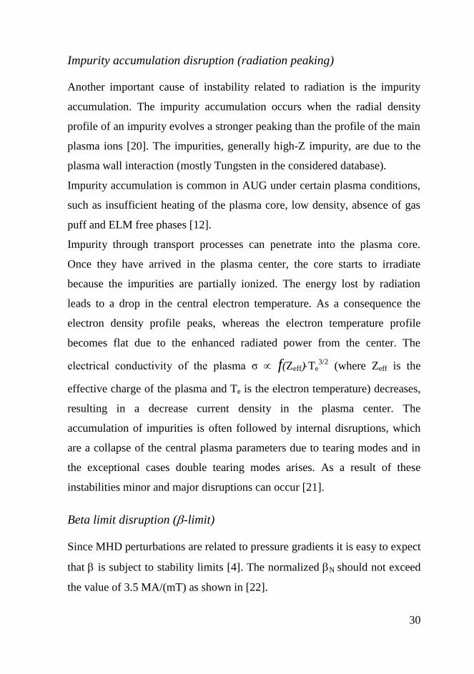
a disruptive label is associated to each sample belonging to the
disruptive phase in a disrupted discharge.
a safe label is associated to each sample belonging to a safe discharge
or to the non-disruptive state of a disrupted discharge in the interval
[tflat-top ÷ tpre-disr] where tflat-top is the flat-top beginning time.
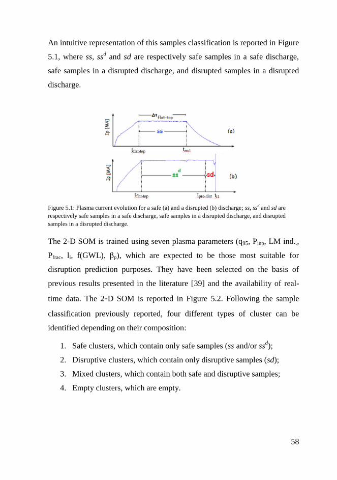
58
An intuitive representation of this samples classification is reported in Figure
5.1, where ss, ssd and sd are respectively safe samples in a safe discharge,
safe samples in a disrupted discharge, and disrupted samples in a disrupted
discharge.
Figure 5.1: Plasma current evolution for a safe (a) and a disrupted (b) discharge; ss, ssd and sd are
respectively safe samples in a safe discharge, safe samples in a disrupted discharge, and disrupted
samples in a disrupted discharge.
The 2-D SOM is trained using seven plasma parameters (q95, Pinp, LM ind..,
Pfrac, li, f(GWL), βp), which are expected to be those most suitable for
disruption prediction purposes. They have been selected on the basis of
previous results presented in the literature [39] and the availability of real-
time data. The 2-D SOM is reported in Figure 5.2. Following the sample
classification previously reported, four different types of cluster can be
identified depending on their composition:
1. Safe clusters, which contain only safe samples (ss and/or ssd);
2. Disruptive clusters, which contain only disruptive samples (sd);
3. Mixed clusters, which contain both safe and disruptive samples;
4. Empty clusters, which are empty.

59
A color has been associated to each cluster of the map depending on the
class membership as shown in Figure 5.2:
Safe clusters are green;
Disruptive clusters are red;
mixed clusters are gray;
Empty clusters are white.
Moreover, each color, which is representative of a particular cluster
composition, can be associated to a different disruption risk.
Since the safe clusters contain only safe samples a low risk of disruption can
be associated to a safe region. Conversely, the disruptive cluster contains
only disruptive samples hence a high risk of disruption can be associated to
disruptive regions. Finally, because the mixed clusters contain several
combinations of safe and disruptive samples, the associated risk of
disruption of each cluster depends on its own composition.
Figure 5.2: 2-D SOM of 7-D AUG operational space, dimension map 1.421 clusters (49x29). Safe
clusters are green, disrupted clusters are red, mixed clusters are gray and empty clusters are white

60
The 2-D SOM reported in Figure 5.2 highlights the presence of a safe region
(green) with an associated low risk of disruption, disruptive regions (red)
with a high risk of disruption and transition regions, which are between the
previous two regions, with an indeterminate risk of disruption.
In addition, Figure 5.3 reports the component plane representation for each
plasma parameter and the 2-D SOM of AUG. The component plane is a tool
available to analyze the SOM results [45]. Component planes display the
relative component distribution of the input data on the 2-D map. By means
of the component planes it is possible to detect if the variables are correlated
to each other and if particular ranges of values are correlate to the disruption
risk. The color bar on the right side of each component plane reports the
range of values of the variable assumed by the prototype vector of the
clusters.
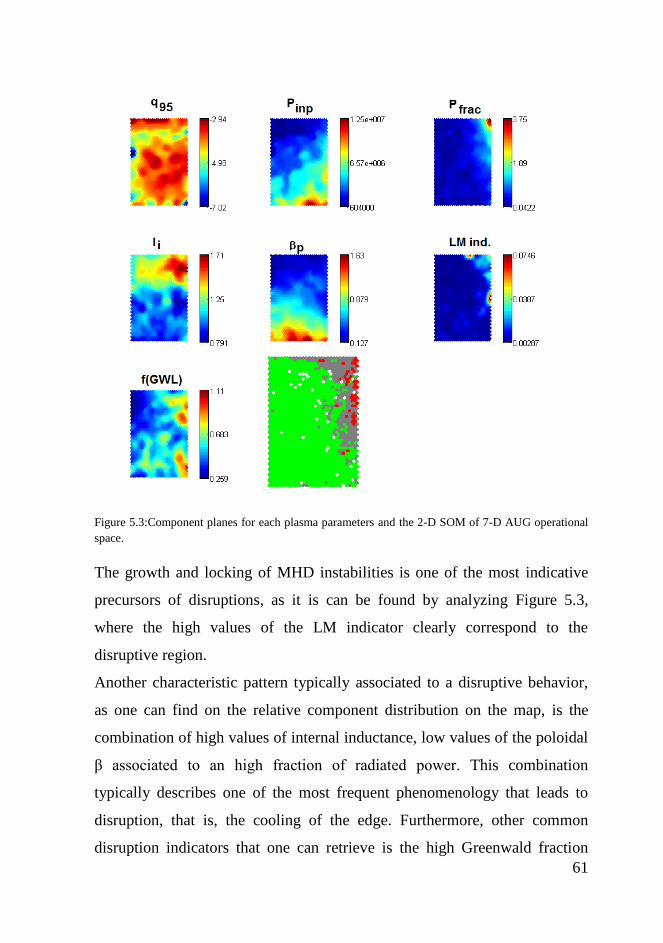
61
Figure 5.3:Component planes for each plasma parameters and the 2-D SOM of 7-D AUG operational
space.
The growth and locking of MHD instabilities is one of the most indicative
precursors of disruptions, as it is can be found by analyzing Figure 5.3,
where the high values of the LM indicator clearly correspond to the
disruptive region.
Another characteristic pattern typically associated to a disruptive behavior,
as one can find on the relative component distribution on the map, is the
combination of high values of internal inductance, low values of the poloidal
β associated to an high fraction of radiated power. This combination
typically describes one of the most frequent phenomenology that leads to
disruption, that is, the cooling of the edge. Furthermore, other common
disruption indicators that one can retrieve is the high Greenwald fraction

62
representative of density limit disruptions, as it is possible to see on the right
side of the SOM, or the low values of edge safety factor and Greenwald
fraction corresponding to the upper part of the map, which are likely
associated to low q95 and low density or EFM disruptions.
Instead, the safe region identifies combinations of the considered plasma
parameters which, if the safe and the disruptive operational spaces are
exhaustively represented, have a low probability to lead to disruption.
5.1.1.1 SOM predictor
As it has been reported in §2.3, disruptions can occur in a tokamak when the
plasma becomes unstable and they can potentially damage plasma-facing
surfaces of the machine. For these reasons, the importance of avoiding
disruptions in tokamaks and/or finding appropriate mitigating actions to
reduce the damage of the reactor components is fundamental for tokamaks
development. In addition, the mitigation system efficiency is linked to its
activation time, this means that the prediction must be made sufficiently in
advance to enable intervention of mitigation systems. Moreover, one of the
main goals of experimental devices, as AUG, is to exploit its own
potentialities. A too conservative disruption predictor could limit the
exploration capability of the machine; in order to avoid this drawback, the
percentage of disruptions triggered too far in advance has to be limited as
well as the false alarms. Finally, the predictor must supply also the
disruption type in order to optimize the strategy to safely land the plasma
and to reduce the probability of damages in the device. Therefore, it is
important and crucial to develop disruption predictors that have specific
characteristics:
The correct predictions of disrupted discharge must be higher than
those of the disruption predictor actually installed in the machine;
63
The number of false alarms must be limited;
The number of missed alarms must be limited;
The prediction system must operate in real time;
The prediction system must predict different disruption types.
In addition to space visualization purposes, the SOM can be used also to
display the time evolution of the discharges during experiments, in fact each
sample of a discharge can be projected onto the SOM; the temporal sequence
of the samples forms a trajectory on the map that describes the discharge
dynamics. The trajectory onto the map can be seen as sequence of points that
represent the Best Matching Units (BMUs). To determine the BMU, one
method is to iterate through all the nodes of the SOM and calculate the
Euclidean distance between each prototype vector and the current sample of
the discharge. The node with the weight vector closest to the current sample
of the discharge is tagged as the BMU.
The analysis of the trajectory can provide information on an eventual
impending disruptive event. In particular, it has been noted that, for the
majority of disruptive discharges, the trajectory starts in the safe region
(green region) and, passing through the transition region, ends in a red
cluster (see the black trajectory in Figure 5.4.). Conversely, the great
majority of safe discharges evolve within the safe region as shown in Figure
5.4. (blue trajectory). Thus, the SOM could be used as disruption predictor
by introducing suitable criteria, based on the behavior of the trajectories,
able to trigger disruption alarms well in advance to perform disruption
avoidance or mitigation actions.

64
Figure 5.4: Trajectories of safe discharge # 20437 (blue trajectory) and disrupted discharge # 21098
(black trajectory) on the 2-D SOM of 7-D AUG.

65
5.1.1.2 Performance indexes
In order to evaluate the performance of the SOM predictor different
performance indexes have been introduced.
A disruption is correctly predicted if the predictor is able to trigger the alarm
in the time interval [tD - 160 ÷ tD - 2] ms. The upper limit depends on the
time needed for the mitigation systems to intervene. At AUG the mitigation
system is able to mitigate a disruption within 2ms [46]. The lower limit is a
conservative value determined on the basis of a locked-mode signal analysis.
In [39], it is shown that more than 90% of disruptive discharges has a
quickly increase of the frequency of oscillation within 160ms before the
disruption.
The performance of the prediction system is evaluated in terms of:
SPs: Successful Predictions, fraction of discharges (disruptive or
safe) that are correctly predicted;
MAs: Missed Alarms, fraction of discharges predicted as non-
disrupted;
PDs: Premature Detections, fraction of disruptive discharges where
the alarm is triggered more than 160ms before the disruption time;
TDs: Tardive Detections, fraction of disruptive discharges where the
alarm is triggered less than 2 ms before the disruption time;
FAs: False Alarms, fraction of safe discharges predicted as
disrupted.
SR: Successful Rate, fraction of discharges (safe and disruptive)
correctly predicted.
A good disruption predictor has to be characterized by high successful
prediction rate and SRs, low PDs and TDs, low MAs and low FAs.

66
5.1.1.3 Alarm criterion
In this thesis, different criteria have been tested to trigger an alarm
monitoring the trajectory followed by the discharge during its temporal
evolution on the map.
A first attempt has been done activating the alarm as soon as the trajectory
passes through the disruptive region of the SOM. Nevertheless, this criterion
has not produced good results due to spikes in the diagnostic signals, which
move the trajectory from the low-risk region to the high-risk region, causing
false alarms or a premature detections.
Furthermore, in order to improve the prediction performance of the SOM
predictor a redefinition of the disruptive region has been carried out,
considering as disruptive clusters also the mixed clusters with a percentage
of disruptive samples greater than 85%.
This has led a new map with a larger disruptive region, as it is shown in
Figure 5.5.
Figure 5.5: 2-D SOM of 7-D AUG operational space. (Green) Safe clusters. (Red) Both disruptive
clusters and those mixed clusters with a percentage of disruptive samples greater than 85%. (Gray)
Other mixed clusters.(White) Empty clusters.

67
In addition, an alarm criteria has been optimized to trigger the alarm when
the trajectory stays in a cluster in the high-risk region for at least k
consecutive samples (waiting samples). Equation (5.1) reports the law which
controls the waiting samples k, in according to the line in Figure 5.6:
100%
%%
MIN
MIN
MINMAX
MAX
DS
DSDS
kk
kk
(5.1)
where DS% is the percentage of disruptive samples in the current cluster and
the line parameters DSMIN%, kMIN and kMAX have been empirically chosen
maximizing the SR on the training set. In order to avoid false or premature
alarms caused by spikes in the diagnostic signals for DS%=100, kMIN has been
set equal to 2, whereas the parameters DSMIN%, kMAX, have been optimized in
the range:
DSMIN %=85÷95
kMAX=15÷30
Figure 5.6: Representation of k law. The disruptive samples percentage (DS%) versus the number of
the waiting samples k.
For each red cluster, the parameter k was evaluated following the linear
relation in (5.1).
The ratio of this alarm criterion is that k inversely decreases with the number
of disruptive samples in the cluster. This means that the bigger is the

68
percentage of disruptive sample in the cluster and the shorter is the trigger
waiting samples.
The best performance on DB1 has been obtained by triggering the alarm
when the trajectory stays in a cluster in the high risk region (red clusters in
the Figure 5.5) for at least 14442.1 % DSk samples. The value of k is
updated only if the trajectory moves into clusters with higher DS%.
Conversely, the alarm is not triggered at all in the low risk region (green and
gray clusters with a percentage of disruptive samples lower than 85%) in
Figure 5.5.
The prediction performances of the proposed system using discharges from
DB1, DB2 and DB3 are reported in Table 5.2. Table 5.2:
Table 5.2: Prediction performances of the SOM for DB1, DB2 and DB3.
Disruptive Discharges Safe Discharges
PD [%] SP [%] TD [%] MA [%] SP [%] FA [%] SR [%]
DB1 9,40 83,89 1,34 5,34 95,00 5,00 87,34
DB2 9,88 65,34 4,94 19,75 90,88 9,12 87,38
DB3 16,95 56,78 5,08 21,19 85,19 14,82 80,03
Note that, as previously explained, the SOM was created using a training set
consisting of a subset of samples from safe and disruptive discharges in
DB1. Test discharges from DB1 therefore belong to the set of experimental
campaigns used for training. Conversely, DB2 and DB3 discharges belong to
later campaigns. Thus, the test on DB2 and DB3 provide information on
generalization abilities of the map. Moreover, the test on DB3 provides
information on the so-called predictor ageing. The ageing effect is common
in experimental machines that operate in ever-changing conditions in order
to explore their potential. The composition of DB3, in terms of disruption
classes, could suggest a possible difference in the operative space explored

69
in the recent years. This is confirmed in [15],where the authors noted that,
until 2008, the large majority of disruptions were of cooling edge type. In
2009, the percentage of cooling edge disruptions decreases to about 45%,
due to the increase of impurity accumulation and β-limit disruptions.
As one might expect, this determines poorer prediction performances on
DB2 and DB3 discharges.
Analyzing the SOM prediction performances reported in Table 5.2, for DB1,
the performances are quite good. The PDs, TDs, MAs and FAs are always
lower than 10%. The SPs on disrupted and safe discharges are respectively
about 84% and 95% respectively. Conversely, for DB2, PDs, TDs, MAs and
FAs always increase with respect to DB1, although PDs and FAs remain
lower than 10%. Also for DB3, PDs, TDs, MAs and FAs increase with
respect to DB1, but in addition PDs and FAs are well above 10%. For both
DB2 and DB3 the SPs for safe and disrupted pulses decrease, confirming the
ageing effect.

70
5.1.1.4 Analysis of false predictions
In order to identify the causes of incorrect predictions, a visual analysis of
the 7 input signals has been performed on DB2. The DB3 has not been taken
into account in this analysis in order to have a test set independent from the
actions that have been adopted.
Firstly, the analysis performed on the correctly predicted disruptions shows
that the large majority of them are triggered in the presence of an increase of
Prad. Moreover, it has been noticed that one of the most common source of
false alarms is the presence of a peak in Pfrac. Therefore, the behavior of the
signals contributing to Pfrac, i.e., Ip, PICRH, PECRH, PNBI, Prad, Uloop, has
been analyzed in order to identify the origin of the Pfrac peak. That analysis
highlighted that 73.5% of false alarms and 50% of premature detections
correspond to the shutdown of one or more additional heating systems that
cause a sudden decrease of the total input power Pinp. This produces a peak
in the Pfrac, which is responsible of triggering the alarm. As an example,
Figure 5.7 reports (a) Pinp and (b) Pfrac for the safe discharge #21011, which
generates a false alarm at 5,01s as a result of the NBI shutdown.

71
Figure 5.7: Time evolution of the Pinp (a) and the Pfrac (b) in the safe discharge # 21011; a sudden
decrease of Pinp generates a peak in Pfrac. The SOM triggers the alarm at 5,01s.
Following trajectories of this kind of discharges on the map, they always
evolve in the region with low disruption risk, except at the peak of Pfrac when
they enter the higher disruption risk region. In Figure 5.8, the trajectory of
the safe discharge # 21011 is reported on the map. The three points in the red
region represent the samples corresponding to the peak of Pfrac. Figure 5.8,
reports also the component planes of Pinp and Pfrac. As highlighted by the
black squares on the component planes, the three points belong to clusters
characterized by low values of Pinp and high values of Pfrac.

72
Figure 5.8: Trajectory of the safe discharge # 21011 on the SOM together with the component planes
of Pinp and Pfrac. The three points in the red region of the SOM represent the samples responsible for
the FA. These three points correspond to low values of Pinp and high values of Pfrac as highlighted by
the black squares on the component planes.

73
5.1.1.5 2-D SOM of 8-D AUG operational space
The analysis performed on the achieved results suggested to provide
additional information to the SOM predictor. Firstly, it has to be noted that a
high value of Pfrac corresponds both to a high value of Prad (nominator of
Pfrac), or to a low value of Pinp (denominator of Pfrac). Hence, the information
curried out by Pfrac could be not adequate to discriminate between the two
cases. For this reason Prad was added to the previous 7 signals of the training
set. Thus, a new SOM was trained with 8 plasma parameters.
In order to train the new map the same issues of the section 5.1.1 were
addressed. In particular, a data reduction is again necessary to balance the
number of safe samples and disruptive samples. The adopted algorithm
reported in [43] allows us to reduce the safe samples to 49.169 starting from
780.969. Also in this case, the tpre-disr has been set equal to 45 ms before the
disruption time, as reported in [39].
The dimension of the map was obtained by means a of trial and error
procedure that maximizes the SR on the training set. The best compromise
results in a map with 2318 clusters (see Figure 5.9) on a 61x38 grid. The
SOM reported in Figure 5.9 shows the same characteristic of the SOM in
Figure 5.5, with the three regions at different disruption risk. The same color
code of Figure 5.5. is adoped in Figure 5.9.

74
Figure 5.9: 2-D SOM of 8-D AUG operational space with the same color code as in Figure 5.5. The
figure displays 2.318 clusters on a 61x38 grid.
In addition, Figure 5.10 reports the component planes representation for each
plasma parameter. Also in this case, it is possible to note that the disruptive
regions are characterized by typical patterns, as the already described
combination of high values of internal inductance, low values of the poloidal
β, high fraction of radiated power and high values of the locked mode
indicator, commonly describing the radiative collapse and cooling of the
edge. Furthermore, similarly to what has been described in the analysis of
Figure 5.3, there are disruptive regions with high values of Greenwald
fraction (left side of the SOM), or still regions that see the combination of
low values of edge safety factor and Greenwald fraction (upper part of the
map), likely associated to low q95 and low density or EFM disruptions.

75
Figure 5.10: Component planes for each plasma parameter and the 2-D SOM of 8-D AUG operational
space.
Secondly, in order to limit false alarms due to a peak of Pfrac, an inhibition
alarm algorithm was implemented, which inhibits the alarm if the following
conditions are simultaneously satisfied:
THR|
dt
dP
dt
dP inpinp at least once in the time window
1 of 20ms preceding the
alarm. The threshold dPinp
dt|THR
=-1.2GW
ms is set as the maximum value
assumed by dPinp
dt, during the shutdown of one or more auxiliary
heating system in the discharges where a FA has been activated by
the shutdown itself.
1 The time windows was optimized among the values [5, 10, 20] ms. The best performance
on DB2are achieved for a time windows of 20 ms.
76
Prad≤Prad|THR
. The threshold Prad|THR
is set as the minimum value
assumed by Prad at the alarm time, for all the correct predictions
performed by the SOM for the DB2 in the presence of an increase of
Prad.
dPrad
dt<
dPrad
dt|THR
.The threshold dPrad
dt|THR
=11MW/ms is the minimum
value assumed by dt
dPrad at the alarm time, for all the correct
predictions performed by the SOM in the presence of an increase of
Prad. dt
dPrad is computed in a time windows of 5 ms.
Hence, an alarm is inhibited in the presence of a peak on Pfrac caused by a
shutdown of the auxiliary heating system, with limited values of Prad and its
derivative.
In order to highlight the influence of adding the signal Prad and that of using
the alarm inhibition criteria (AI) the prediction performances of the 7-D and
8-D SOMs are reported in Tables 5.3, 5.4 and 5.5, for DB1, DB2 and DB3
respectively, without and with AI. The alarm criterion is the same described
in section 5.1.1.3. The best performance on DB1 has been obtained by
triggering the alarm when the trajectory stays in a cluster in the high-risk
region for at least 44.77754.0 % DSk consecutive samples. Whereas,
the alarm is not triggered at all in the low risk region (green and gray cluster
with a percentage of disruptive samples lower than 85%) in Figure 5.9.
Table 5.3:.

77
Table 5.3: Prediction performances of the SOMs of the 7-D and 8-D operational spaces of AUG on
DB1.
Disruptive Discharges Safe Discharges
DB1 PD [%] SP [%] TD [%] MA [%] SP [%] FA [%] SR [%]
7-D 9.40 83.89 1.34 5.34 95.00 5.00 87.34
8-D 11,41 86,58 0,67 1,34 96,25 3,75 92.87
able 5.4:
Table 5.4: Prediction performances of the SOMs of the 7-D and 8-D operational spaces of AUG with
and without alarm inhibition algorithm (AI) on DB2.
Disruptive Discharges Safe Discharges
DB2 PD [%] SP [%] TD [%] MA [%] SP [%] FA [%] SR [%]
7-D 9,88 65,43 4,94 19,75 90,88 9,12 87,54
8-D 11,11 69,14 6,17 13.58 91,25 8.75 88,35
7-D+AI 8,64 66,67 4,94 19,75 94,04 5,96 90,45
8-D+AI 9,88 69,14 6,17 14,81 93,85 6,15 90,61
Table 5.5:
Table 5.5: Prediction performances of the SOMs of the 7-D and 8-D operational spaces of AUG with
and without alarm inhibition algorithm (AI) on DB3.
Disruptive Discharges Safe Discharges
DB3 PD [%] SP [%] TD [%] MA [%] SP [%] FA [%] SR [%]
7-D 16,95 56,78 5,08 21,19 85,18 14,82 80,03
8-D 11,02 66,95 7,63 14,40 85,37 14,63 82,03
7-D+AI 14,41 59,32 5,08 21,19 87,24 12,76 82,18
8-D+AI 8,47 69,50 7,63 14,40 87,05 12,95 83,87
The comparison among the previous tables shows that, by adding the signal
Prad to the SOM inputs, a reduction of MAs and an increase of SPs for safe
and disrupted discharges are achieved for DB1, DB2 and DB3 (see Tables
5.3-5.5). Note that, however, this does not always bring a benefits for the
reduction of FAs and PDs (Tables 5.3-5.5). Analyzing the performances on

78
DB2 reported in Table 5.4, adding the Prad in the training set causes an
increase of the PDs with respect to the PDs of the 7-D predictor.
On the contrary, the use of AI leads to significant reductions of PDs, FAs and
MAs, for both the two test sets (DB2 and DB3). But any positive effect on
TDs is achieved. It seems that the use of both criteria together (adding Prad
and AI) gives the better performance. This is confirmed by comparing the
total prediction success rate (SR). Referring to DB2, the total prediction
success rate grows from 87,54% for 7-D SOM predictor, to 88,35%, for the
8-D, to 90.45% for 7-D + AI, and, to 90,61% for the 8-D+AI. Referring to
DB3, the total prediction success rate grows from 80,03% for 7-D SOM
predictor, to 82,03% for the 8-D, to 82,18% for the 7-D +AI, to 83,87% for
the 8-D+AI.

79
5.1.1.6 Retraining of the 8-D AUG operational space
The results obtained in the previous section (5.1.1.5) shows a quite good
prediction success rates, which degrades with the temporal distance of the
considered campaigns from those included in the training. As largely known,
the ageing effect is one of the main drawbacks of the data-based models,
such as SOM.
In order to improve the extrapolation capability of the SOM predictor, which
is intrinsically poor when the inputs come from regions of the parameters
space different from those used during the training, further knowledge has to
be supplied regarding these regions. This can be performed occasionally
retraining the SOM, supplying it new data coming from discharges that
correspond to wrong answers of the predictor. In this way, the map can learn
incrementally from new data as the operational space is enlarged with
respect to the prior campaigns. Following this philosophy, a new training
session has been performed providing to the SOM the MAs, TDs, PDs and
FAs triggered when the SOM is tested on the DB2 discharges. In case of
PDs and FAs all samples that belong to the time window of 20 ms before the
alarm is used for updating. Furthermore, in case of MAs the samples useful
for the updating are selected by means of the data reduction procedure
(explained in § 5.1.1), in this way novel information of safe and disrupted
states are added to the training set.
As previously cited, the analysis of the wrong answers of DB2 highlighted
that the great majority of false alarms and half of premature detections
correspond to the shutdown of one or more auxiliary heating systems that
cause a sudden decrease of the total input power Pinp. This produces a peak
in the Pfrac, which is responsible of triggering an alarm even if Prad has low
values (this analysis is reported in § 5.1.1.4). For this reason, these pulses are
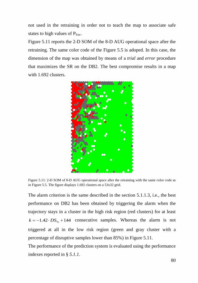
80
not used in the retraining in order not to teach the map to associate safe
states to high values of Pfrac.
Figure 5.11 reports the 2-D SOM of the 8-D AUG operational space after the
retraining. The same color code of the Figure 5.5 is adoped. In this case, the
dimension of the map was obtained by means of a trial and error procedure
that maximizes the SR on the DB2. The best compromise results in a map
with 1.692 clusters.
Figure 5.11: 2-D SOM of 8-D AUG operational space after the retraining with the same color code as
in Figure 5.5. The figure displays 1.692 clusters on a 53x32 grid.
The alarm criterion is the same described in the section 5.1.1.3, i.e., the best
performance on DB2 has been obtained by triggering the alarm when the
trajectory stays in a cluster in the high risk region (red clusters) for at least
14442.1 % DSk consecutive samples. Whereas the alarm is not
triggered at all in the low risk region (green and gray cluster with a
percentage of disruptive samples lower than 85%) in Figure 5.11.
The performance of the prediction system is evaluated using the performance
indexes reported in § 5.1.1.

81
Tables 5.6 and 5.7 report the prediction performance of the SOM used as
disruption predictor for DB2 and DB3 respectively before (these results are
reported in § 5.1.1.5) and after the retraining.
Table 5.6:
Table 5.6: Prediction performances of the 2-D SOM of the 8-D AUG operational space on DB2 before
and after the retraining.
Disruptive Discharges Safe Discharges
DB2 PD [%] SP [%] TD [%] MA[%] SP [%] FA [%] SR [%]
Before the
Retraining 11,02 66,95 7,63 14,40 85,37 14,63 82,03
After the
Retraining 10,13 73,42 3,80 12,66 93,31 6,69 90,70
Table 5.7:
Table 5.7: Prediction performances of the 2-D SOM of the 8-D AUG operational space on DB3 before
and after the retraining.
Disruptive Discharges Safe Discharges
DB3 PD [%] SP [%] TD[%] MA[%] SP [%] FA [%] SR [%]
Before the
Retraining 11,02 66,95 7,63 14,41 85,37 14,63 82,03
After the
Retraining 9,32 68,64 7,63 14,41 89,12 10,88 84,65
As it can be noted, comparing Tables 5.6 and 5.7, for both DB2 and DB3,
the successful predictions (SP) after the retraining, increases for both safe
and disruptive discharges. It seems that the use of periodically retraining
gives the better performance. This is confirmed by comparing the total
prediction success rate (SR). Referring to DB2, the total prediction success
rate grows from 82,03% before the retraining, to 90,70% after the retraining.
Referring to DB3, the total prediction success rate grows from 82,03% before
the retraining to 84,65% after the retraining.

82
Moreover, the suitability of the proposed updating procedure is confirmed
making reference to DB3: due to the ageing, the overall performance slightly
deteriorates with respect to that of DB2, but the prediction success rates are
still high.

83
5.1.2 Normal operating conditions model of ASDEX Upgrade
In the last decade, the disruption prediction issue has been investigated in
various tokamaks resorting to data-based approaches such as neural
networks, support vector machines, fuzzy logic, classification and regression
trees[15, 39, 42, 47-48]. One of the main drawbacks of all the data-based
model proposed in literature, as well as in section 5.1.1 and in the later of
this thesis, is the need of a dedicated set of experiments terminated with a
disruption to implement the predictive model For future fusion devices, like
ITER, disruptions associated damages could be even more severe because of
the much higher plasma current of the devices. Hence, the disruption
database will not be available. Thus, previously cited approaches will not be
directly applicable.
In this thesis, in order to overcome the previous highlighted drawbacks, a
disruption prediction system for AUG is proposed using only input signals
from safe pulses. The proposed approach refers to the model-based methods
for Fault Detection and Isolation (FDI) in batch processes [49]. Indeed, the
current experimental tokamak machines operate in a discontinuous or pulsed
way and individual pulses can be seen as a single batch. FDI is an important
and active research field. Literature reports several techniques for detecting
faults such as observers, parity space methods, eigen structure assignments,
parameter identification based approaches, etc (see the survey of [50] for a
recent review). The majority of the model-based FDI procedures are based
on statistical analysis of residuals. Commonly, the residual is the difference
between the measured output and an estimated output based on the system
model. Given an empirical model identified on a reference dataset, obtained
under normal operating conditions (NOC), the residuals of new observations
of the current process run are calculated. The residuals are considered as a

84
random process with known statistical properties. In case of fault there is a
change of these properties.
A number of approaches have been developed for fault diagnosis and
identification of batch processes that are commonly used in many industrial
sectors. They are characterized by the repeated execution of a planned
schedule over a finite duration of time. Most recent researches apply
Principal Component Analysis (PCA) based techniques [31, 51]. The Multi-
way PCA is the standard way to analyze batch data [52] that are inherently
three-dimensional (batch×variable×time), Batch Dynamic PCA [53] to take
into account the dynamic of the batch process; Auto-Regressive PCA [54] to
filter auto and cross correlations.
In this thesis, the safe pulses are assumed as the normal operation conditions
and the disruptions are assumed as status of fault. The disruption prediction
system is based on the analysis of residuals in the multidimensional space of
the selected variables, which are able to describe the safe operational space
of the tokamak. An Auto Regressive eXogenous input (ARX) model is used
as predictor for the variables; the discrepancy (residuals) between the outputs
provided by the NOC model and the actual measurements is an indication of
process fault (disruption).
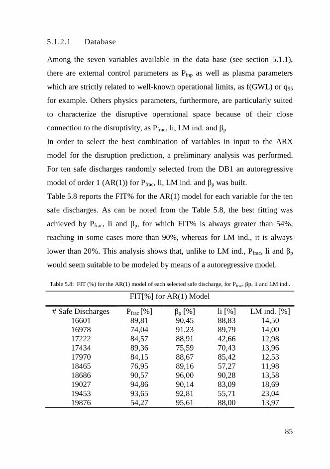
85
5.1.2.1 Database
Among the seven variables available in the data base (see section 5.1.1),
there are external control parameters as Pinp as well as plasma parameters
which are strictly related to well-known operational limits, as f(GWL) or q95
for example. Others physics parameters, furthermore, are particularly suited
to characterize the disruptive operational space because of their close
connection to the disruptivity, as Pfrac, li, LM ind. and βp
In order to select the best combination of variables in input to the ARX
model for the disruption prediction, a preliminary analysis was performed.
For ten safe discharges randomly selected from the DB1 an autoregressive
model of order 1 (AR(1)) for Pfrac, li, LM ind. and βp was built.
Table 5.8 reports the FIT% for the AR(1) model for each variable for the ten
safe discharges. As can be noted from the Table 5.8, the best fitting was
achieved by Pfrac, li and βp, for which FIT% is always greater than 54%,
reaching in some cases more than 90%, whereas for LM ind., it is always
lower than 20%. This analysis shows that, unlike to LM ind., Pfrac, li and βp
would seem suitable to be modeled by means of a autoregressive model.
Table 5.8:
Table 5.8: FIT (%) for the AR(1) model of each selected safe discharge, for Pfrac, βp, li and LM ind..
FIT[%] for AR(1) Model
# Safe Discharges Pfrac [%] βp [%] li [%] LM ind. [%]
16601 89,81 90,45 88,83 14,50
16978 74,04 91,23 89,79 14,00
17222 84,57 88,91 42,66 12,98
17434 89,36 75,59 70,43 13,96
17970 84,15 88,67 85,42 12,53
18465 76,95 89,16 57,27 11,98
18686 90,57 96,00 90,28 13,58
19027 94,86 90,14 83,09 18,69
19453 93,65 92,81 55,71 23,04
19876 54,27 95,61 88,00 13,97

86
Data for this test were selected from experimental campaigns performed
between July 2002 and November 2009 and it has been divided in three
subsets following the temporal progress as reported in Table 5.9.
Table 5.9:
Table 5.9: Database composition.
Safe pulses Disrupted pulses
Training Validation Test Test
DB1 37 19 17 149
DB2 - - 537 81
DB3 - - 533 118
Some safe pulses of the DB1 was used for the training of the ARX model,
the validation set was used to optimize the characteristic of the predictor as it
is explained later and finally the rest of DB1 was used to test the ARX
predictor. As can be noted, disruptive discharges of DB1 were used only as
test set. DB2 was used to test the generalization capability of the model,
finally DB3 was used to evaluate the performance of the model with
discharges belonging to later campaigns. The safe and disruptive discharges
are the same discharges used to evaluate the prediction performance of the
SOM predictors shown in the § 5.1.1 and in the later.
The dataset is composed by time series related to Pfrac, li and βp. The reason
to use only three variables is to have a graphical representation of the
process and hence to verify the correct functioning of the model.
5.1.2.2 NOC model of ASDEX Upgrade
The NOC model of AUG was built using 37 training discharges of DB1. For
each plasma parameter, the dynamic structure of each pulse is estimated
through the fitting of an ARX model, which uses as inputs the three selected
plasma parameters and provides as outputs one plasma parameter at once,
one step ahead. In particular, the ARX model for each variable is built
according to equation (4.3) reported in chapter 4. As an example,

87
considering Pfrac as output variable and li and βp as exogenous inputs, the
equation 4.3 becomes as in the following:
21
1
22
1
11
1
)()()()(bba n
i
i
n
i
pi
n
i
fracifrac nkitlibnkitbitPatP
(5.2)
Therefore, for each of the tree models, na, is the order of the output variable,
nb=[nb1, nb2], contains the orders of the exogenous inputs, ai, bi1 and bi2 are
vectors that contain the model coefficients of the three variables and
nk=[nk1, nk2] is the vector of the time delay. To estimate the ARX structures,
the parameters na, nb and nk must be specified. In this study, the three
parameters have been set as those corresponding to the best fit on the
validation set. In particular, an ARX model for each model order and time
delay combination is estimated. Then, the loss function, which is the
normalized sum of squared prediction errors, for each model is calculated.
The best fit minimizes the loss function on the validation set. The delays and
the orders have been optimized in the range [1-40] and [1–20] respectively.
Moreover, the coefficients ai,bi1 and bi2 in the ARX model structure have
been estimated with the least-squares method, which minimizes the loss
function provided by the model on the same validation set. In this thesis the
model order, the time delay and the model coefficients have been optimized
using the System Identification toolbox for Matlab [32].
The NOC model for each plasma parameter is still an ARX model whose
coefficients are obtained as mean value of coefficients of the 37 ARX
models of the training shots. Table 5.10 reports the NOC model orders
associated to the different outputs related to the three inputs.

88
Table 5.10:
Table 5.10: Model orders associated with the different outputs and inputs.
na nb1 nb2 nb3
Pfrac 20 - 57 48
li 20 48 - 31
βp 20 31 20 -
Once the NOC model has been built, it can be used for pulses monitoring.
Indeed, sample by sample NOC model output depicts the simulated
trajectory of the discharge in the 3-D space Pfrac, li and βp. As an example,
Figure 5.12. reports the actual and the simulated temporal evolution in the 3-
D space for the disrupted pulse # 16220 (a) and for the safe pulse # 16863
(b). As can be noted, for the safe pulse the two trajectories (red and blue
line) are always overlapped. Conversely, for a disrupted discharge the more
the disruption time approaches the more the two trajectories diverge. This
suggested to use the discrepancy between the predicted and the actual values
as disruption proximity indicator.
Therefore, the residuals of the actual values from the NOC models are used
for monitoring the pulses. In particular, the residuals are assumed as the
Euclidean distances between the position of the samples on the actual pulse
trajectory in the 3-D parameter space, and the corresponding positions
simulated with the three NOC models. Figure 5.13 reports the time evolution
of the residual for the same disrupted (a) and safe (b) discharges in Figure
5.12. As can be noted for the safe discharge the residual assumes always a
low values for the entire duration of the experiment (Figure 5.13 (b), green
line) while for the disrupted discharge, the residual starts and evolves with
low values and rapidly it increases close to the disruption.

89
Figure 5.12: Actual (blue line) and the simulated NOC model output (red line) temporal evolution in
the 3-D space for the disrupted pulse # 16220 (a) and for the safe pulse # 16863 (b).

90
Figure 5.13: Time evolution of the residual for (a) the disrupted discharge #16220 (blue line) and (b)
the safe discharge #16863 (green line).
The aim is to identify the pre-disruptive phase evaluating the distance of the
simulated shot trajectory in the 3-D space from the actual one. In order to
detect the disruptive phase for a disrupted pulse it is necessary to find a
residual threshold which discriminates between the non-disruptive and the
disruptive phase.
In this thesis, the choice of the residual threshold has been carried out on
training and validation sets of DB1 (see Table 5.9). Figure 5.14 reports the
standardized distribution of the residuals of the training and validation
discharges. In order to find the optimal residual threshold, a confidence limit
of 99% has been empirically assumed to discriminate between the non-
disruptive and the disruptive phase, and the alarm threshold has been set
accordingly.

91
Figure 5.14: Distribution of the residuals of the training and validation sets.
To avoid false alarms caused by spikes in the diagnostic signals, a time delay
has been introduced that inhibits the alarm for k consecutive samples after
that the alarm is activated. The parameter k has been optimized in the range
[1÷10]. The optimal value of k is evaluated maximizing the prediction
performance calculated on validation set (reported in Table 5.11).
In order to evaluate the prediction performance of the predictor the same
performance indices introduced in section 5.1.1.2 have been adopted.
The best performances are obtained triggering the alarm when the residual is
greater than the alarm threshold for at least k consecutive samples. The
minimum value of k that maximizes the performance on validation set is
equal to 5 samples.

92
Table 5.11:
Table 5.11: Prediction performances of the NOC predictor on validation set.
k SP [%] FA [%]
1 5,26 94,74
2 21,05 78,95
3 26,36 73,68
4 68,42 31,58
5 89,47 10,53
6 89,47 10,53
7 89,47 10,53
8 89,47 10,53
9 89,47 10,53
10 89,47 10,53
The performances of the NOC model as disruption predictor on DB1, DB2
and DB3 are reported in Table 5.12.
Table 5.12:
Table 5.12: Prediction performances of the NOC model on DB1, DB2 and DB3.
Disruptive Discharges Safe Discharges
k=5 PD [%] SP [%] TD [%] MA [%] SP [%] FA [%] SR [%]
DB1 10,07 77,18 1,34 11,41 100 0 79.51
DB2 18,52 64,20 3,70 13,58 77,28 22,72 65,91
DB3 18,64 72,03 0,00 9,32 75,61 24,39 72,68
The prediction performances of the proposed method are quite encouraging,
considering that the model is trained with only safe pulses. For DB1 the
successful prediction on safe pulses is 100% and the successful prediction on
disrupted pulses is greater than 77%.
Note that, as previously explained, the NOC model was created using a
training set from safe discharges of the DB1. Test discharges from DB1

93
therefore belong to the set of experimental campaigns used for training.
Conversely, DB2 and DB3 discharges belong to later campaigns. Indeed, as
shown in Table 5.12 the performances of the NOC model, for DB2 and DB3,
deteriorates. The PDs and the FAs for DB2 and DB3 increase with respect to
the PDs and FAs of DB1. Referring to DB2, the total prediction success rate
decreases from 79.51% for DB1 to 65.91%, whereas, for DB3 the total
prediction success rate decreases from 79.51% for DB1 to 72.68%.
Figure 5.15 reports a histogram giving the cumulative distribution of the
warning times tD−talarm for DB1, where talarm is the alarm time. The
percentage is referred to the total number of alarms triggered by the system
on disrupted pulses. The stem corresponding to a warning time greater than
160 ms includes also the premature detections. As can be noted, because at
AUG 2 ms are sufficient for the protection system to intervene, in 98.5% of
the cases the alarm is given enough in time.
Figure 5.15: Cumulative histogram of the warning time (tD − talarm) between the disruption time and the
alarm time, for DB1.

94
5.1.2.3 Analysis of false predictions
As highlighted in section 5.1.1.4 one of the most common sources of
incorrect predictions on DB2 is the shutdown of one or more auxiliary
heating systems that causes a sudden decrease of the Pinp. This produces a
peak in the Pfrac, which is responsible for increasing the residual and for
triggering the alarm. As an example, the same pulse analyzed in section
5.1.1.4 is taken into account. Figure 5.16 reports Pinp, Pfrac and the NOC
residual, for the safe discharge # 21011. An increase of the residual well
above the alarm threshold is recorded in correspondence to the Pinp drop-off,
which generates a false alarm at 5.01s as a result of the NBI shutdown.
Figure 5.16: Discharge # 21011: a) Pinp; b) Pfrac; c) the corresponding NOC model residual
In order to limit the wrong predictions due to a peak of Pfrac, the same
algorithm proposed in section 5.1.2, which inhibits the system alarm in the
presence of a peak on Pfrac caused by a shutdown of the auxiliary heating
systems has been adopted.
Tables 5.13 and 5.14 report the prediction performances of the NOC model
on DB2 and DB3, without (first row) and with (second row) the alarm
inhibition (AI) algorithm respectively.

95
Table 5.13:
Table 5.13: Prediction performances of the NOC model without and with alarm inhibition algorithm
(AI) on DB2.
Disruptive Discharges Safe Discharges
DB2 PD [%] SP [%] TD [%] MA [%] SP [%] FA [%] SR [%]
without
AI 18,52 64,20 3,70 13,58 77,28 22,72 65,91
with
AI 9,88 70,37 4,94 14,81 87,15 12,85 72,57
Table 5.14:
Table 5.14: Prediction performances of the NOC model without and with alarm inhibition algorithm
(AI) on DB3.
Disruptive Discharges Safe Discharges
DB3 PD [%] SP [%] TD [%] MA [%] SP [%] FA [%] SR [%]
without
AI 18,64 72,03 0,00 9,32 75,61 24,39 72,68
with
AI 13,56 76,27 0,00 10,17 84,62 15,38 77,78
The use of AI leads to significant reductions of PDs and FAs, on both the two
data sets (DB2 and DB3). But any positve effect on TDs and MAs is
achieved. However, it seems that the use of the AI criteria gives the better
performances. This is confirmed by comparing the total prediction success
rate (SR). Referring to DB2, the total prediction success rate grows from
65.91% for the ARX NOC model without AI, to 72.57% for the NOC ARX
with AI. Referring to DB3, the total prediction success rate grows from
72.68% for the ARX NOC model without AI, to 77.78% for the NOC ARX
with AI.
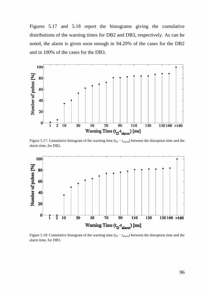
96
Figures 5.17 and 5.18 report the histograms giving the cumulative
distributions of the warning times for DB2 and DB3, respectively. As can be
noted, the alarm is given soon enough in 94.20% of the cases for the DB2
and in 100% of the cases for the DB3.
Figure 5.17: Cumulative histogram of the warning time (tD − talarm) between the disruption time and the
alarm time, for DB2.
Figure 5.18: Cumulative histogram of the warning time (tD − talarm) between the disruption time and the
alarm time, for DB3.

97
5.1.3 Conclusions
A 2-D SOM of the 7-D plasma parameter space has been built for AUG. The
map has been used as disruption predictor by analyzing the trajectories
described over the map by the discharges under test. The performance has
been evaluated using the data coming from experimental campaigns different
and temporally far from those used to build the SOM.
In order to improve such performance, the results have been analyzed with
reference to the wrong predictions. It has been found that high values of Pfrac,
due to the shutdown of the auxiliary heating systems are responsible for most
of FAs and PDs. In order to reduce this problem, two actions have been
undertaken: adding Prad to the SOM inputs and introducing an inhibition
alarm algorithm. These have leaded to an increase of the performance for
both on DB2 and DB3.
Moreover, in order to reduce the ageing effect of the mapping a periodically
retraining of the SOM has been proposed. In particular, the SOM has been
updated using data from wrong predictions on pulses from DB2. The
updated SOM has been tested over DB3. This last test is important as the
deterioration of the generalization capability across campaigns is one of the
main drawbacks of data-based approaches. There is an improving of the
performance confirming the appropriateness of a retraining phase; the
prediction success rate on disruptive discharges is about 69%, and greater
than 89% on safe discharges
Finally, a new view on disruption prediction using a well-tested industrial
technique, the FDI approach, has been proposed. The main advantage with
respect to the SOM is the fact that the model does not need disruptions to
train the system but only a limited number of safe pulses. In addition this
method is suitable to be applied in future devices, such as ITER, which must
tolerate only a limited number of disruptive events and hence a large

98
database of disrupted discharges is not available. The prediction is based on
the analysis of the residuals of an Auto Regressive eXogenous input model
(ARX) built using Pfrac, li and βp. The prediction performance of the
proposed system is encouraging when it is applied on DB1. However, the
false alarms significantly increase when the system is tested on discharges
coming from DB2 and DB3. In order to reduce this problem, the inhibition
alarm algorithm proposed for the SOM has been adopted with good
improvements on the total success rate.
Note that, the computational time required to generate the ARX models
using the System Identification Toolbox of Matlab [55] is about few
minutes, but it is an off-line operation, as well as training a SOM by means
the SOM toolbox running in Matlab. During on-line operation the ARX
predictor only calculates the residuals and compares them with the threshold.
Whereas the SOM predictor only calculates the Euclidean distance among
the considered sample and the prototype vectors and assigns it to the closest
one. These operations are quite fast and well below the signal sampling time
of 1ms.

99
5.2 Database 2007-2012
In order to confirm the validity of the manifold learning methods to serve as
disruption predictors a new data base has been considered, which contains
safe and disrupted discharges selected from experimental campaigns
performed at AUG between May 2007 and November 2012, hence
containing data from more recent campaigns.
The choice of May 2007 as starting point of the new database has been made
because significant changes in the machine configuration have been done. In
particular, the ASDEX Upgrade carbon wall and divertor have been replaced
in a stepwise manner by full W-wall [56]. It is known that the plasma
behavior is directly connected to the plasma-wall interaction and then also
disruptions are affected from this modification. Hence, the new database
contains both all discharges (safe and disrupted) in the pulse range
[21654÷22146] of the DB2 and all pulses (safe and disrupted) of the DB3 (as
labeled in Table 5.1). Moreover, it contains also safe and disrupted pulses
from the experimental campaigns performed from December 2009 to
November 2012.
The shots selection for the creation of the database followed the criteria
reported in section 5.1.1. Briefly, only those disruptions which occurred in
the flat-top phase or within the first 100ms of the plasma ramp-down phase
and characterized by a plasma current greater than 0.8MA are considered.
Moreover, disruptions mitigated by massive gas injection (both those
triggered by the locked mode alarm, and those performed as valve test), and
those caused by vertical instabilities, were excluded. The composition of the
new database is reported in Table 5.15.

100
Table 5.15: Composition of the new database (time period May 2007-November 2012)
Data set Safe pulses Disrupted pulses Time Period
Training Set 291 77 May 2007- April 2011
Test 1 145 72 May 2007- April 2011
Test 2 254 82 May 2011- April 2012
Each of the three datasets is composed of time series related to the following
plasma parameters:
1. Ip: plasma current [A]
2. q95:safety factor at 95% of poloidal flux [a.u.]
3. Pinp: total input power [W]
4. LM ind.: locked-mode indicator [V].
5. Prad: radiated power [W]
6. f(GWL): Greenwald fraction [AU]
7. βp: poloidal β [AU]
8. li: internal inductance [AU]
All signals are sampled making reference to the time base of the plasma
current and the sampling rate is equal to 1kHz.
Discharges performed from May 2007 to April 2011 has been used to train
the models (Training Set). The Test 1 has been built with shots performed in
the same time period of the Training Set, but not included in the Training
Set. It has been used to test the generalization capability of the models.
Finally the Test 2, containing shots successive to those in the Training Set,
has been used to evaluate the ageing of the models when used during more
recent campaigns.

101
5.2.1 Mapping of the ASDEX Upgrade operational space using GTM
and SOM
As previously highlighted, the identification of the boundaries of the
disruption free plasma parameter space would lead to an increase of the
knowledge of disruptions. A viable approach to understand the disruptive
events consists in extracting information from the complex multidimensional
operational space, of the machine and to assume those data, which describe
this space lie on an embedded, low-dimensional sub-space (manifold) within
the higher dimensional space. Manifold learning algorithms attempt to find a
low-dimensional representation of the data [57]. Once the low-dimensional
representation of the data is carried out, the exploratory data analysis
techniques can be useful in order to identify if the parameters used to
describe the plasma operational space are correlated to each other or to
detect the most important variables or if particular ranges of the variables are
associated to the disruption risk.
In the section 5.1 of this thesis a first manifold learning method has been
presented, the Self Organizing Map (SOM). The SOM trained with non-
disrupted and disrupted pulses has been used to display the AUG operative
space in order to identify regions with high risk of disruption and those with
low risk of disruption. In addition to space visualization purposes, the SOM
has been used also to monitor the time evolution of the discharges during an
experiment. The SOM has been used as a disruption predictor achieving
good results.
In this second part of the thesis another manifold learning technique has been
investigated, the Generative Topographic Mapping (GTM). Moreover, for
comparison purposes in terms of mapping and prediction performances, a
SOM is again developed.

102
5.2.1.1 Data reduction
Being each signal sampled at 1 kHz, a huge amount of data (about 1M
samples) is available for describing the safe operational space. The number
of samples in safe pulses together with those belonging to the safe phase of
disruptive shots is much larger than the number of samples available in the
disruptive phase. For this reason, in order to balance the number of safe and
disruptive samples and in order to reduce the computational effort during the
GTM and the SOM training phase, a data reduction of the safe samples
aimed to select only a limited number of significant samples has been
performed. In this case, conversely to the data reduction procedure reported
in section 5.1.1, the data reduction algorithm is applied only to the safe
discharges. Because it is widely shared by the fusion community that the
non-disruptive phase of disruptive shots is well represent by the safe pulses.
Hence, only samples belonging to the safe discharges have been considered
to describe the non-disruptive configurations as also assumed in [15].
The data reduction has been performed by means of a SOM built using the
safe samples belonging to the safe discharges in the training set. A limited
number of samples for each cluster have been selected. Once the SOM is
trained, each cluster will contain only samples supposed to have similar
features. Then, for each not empty cluster at most three samples have been
retained.
In Figure 5.19 a generic cluster of the SOM is visualized. The black point
represents the cluster prototype vector, the red and the blue points are the
samples with the smallest and greatest Euclidean distance from the cluster
prototype vector respectively. The green point is the closest to the
intermediate Euclidean distance between the green and the red ones. The red,
the green and the blue points have been selected during the data reduction
procedure whereas the black and the gray points have been discarded.

103
Figure 5.19: Generic cluster of the SOM. The black point is the prototype vector, the red, the green
and the blue points are the samples with the smallest, the closest to the intermediate and greatest
Euclidean distance from the cluster prototype vector, respectively. The black and the gray points are
the samples not selected during the data reduction.
Following this criteria only 2.6% of the training safe samples has been
retained, reducing the number of samples from 1.030.018 to 26.640.

104
5.2.2 SOM & GTM predictors
The training phase of the SOM and GTM predictors is based on the
availability of a set of disrupted and a set of non-disrupted discharges. The
non-disrupted set is composed of safe samples while the disruptive set is
composed of all samples taken in the time interval [tpre-disr ÷ tD] of the
selected disrupted discharges. Even in this training phase, as that in section
5.1.1., the time instant tpre-disr has been chosen equal for all disrupted
discharges. For AUG discharges, the optimal value of tpre-disr is set equal to
45 ms before the disruption time, as it suggested in the literature [39].
As it was done in section 5.1.1, during the training of both GTM and SOM,
further knowledge has been added to the intrinsic knowledge contained by
plasma parameters, which consists in associating a label to each sample in
the training set:
a disruptive state is associated to each sample belonging to the
disruptive set.
a safe state is associated to each sample belonging to the safe
discharges.
The Min-Max normalization between 0 and 1 has been adopted to train the
GTM and the Z-score standardization has been adopted to train the SOM.
The Z-score standardization, widely used in statistics, consists to convert a
distribution x with mean µ and standard deviation σ to a new distribution
with zero mean and standard deviation equal to one, i.e., if x is a generic
plasma variable of the training set, the Z-score standardization is computed
as:
σ
μ
xx scorez
(5.2)
For the two maps, the normalization/standardization type has been chosen
maximizing the SR on the Training Set.

105
In this thesis, the SOM Toolbox 2.0 for Matlab [45] has been used to train
the SOM, while the exploratory data analysis toolbox for Matlab [58] and
the extension of this toolbox [27] have been used to train the GTM.
As illustrated in section 5.1.1, the 2-D SOM was trained using seven plasma
parameters (q95, Pinp, LM ind., Pfrac, li, f(GWL), βp), but in this second
database Pfrac=Prad/Pinp has been excluded in order to reduce the ambiguous
information provided to the models. This ambiguity is due to the fact that
high values of Pfrac may correspond both to a high values of Prad (nominator
of Pfrac), or to low values of Pinp. These latest are determined by the
shutdown of one or more additional heating systems that cause a sudden
decrease of the total input power Pinp. In the § 5.1.1.4 and 5.1.2.3 it has been
shown that the most common source of incorrect predictions is the shutdown
of one or more auxiliary heating systems that causes a sudden decrease of
Pinp. This produces a peak in Pfrac, which is responsible for triggering the
alarm. For these reason, Pfrac has been replaced with Prad.
The number of clusters in the SOM is chosen by using the heuristic formula
K=5*N0.54321
, which is suggested as default in the SOM Toolbox 2.0 [45],
where N is number of the training samples. As the tool used to train the
GTM implements only squared maps, the number of cluster in the GTM has
been chosen as the square of an integer closest to the number of clusters in
the SOM.
For both maps the same type of clusters reported in §5.1.1 can be identified
and the same colors code used in Figure 5.2 has been associated to each
cluster. Moreover, to each cluster composition a different disruption risk can
be associated, as already done in section 5.1.1.
Figure 5.20 reports the 2-D GTM (a) and the 2-D SOM (b) of the 7-D AUG
operational space. The number of clusters is equal to 1.396 for the GTM and
1.364 for the SOM.

106
Figure 5.20: (a) 2-D GTM (37x37 clusters), (b) 2-D SOM (44x31 clusters) of 7-D AUG operational
space. Safe clusters are green, disrupted clusters are red, mixed clusters are gray and empty clusters
are white. Figure 5.20:
In both maps the safe regions (green) identify combinations of the
considered plasma parameters that, if the overall operational space is
exhaustively represented, have a low probability to lead to a disruption.
Furthermore, in both maps there are several disruptive regions (in red) with
an associated high-risk of disruption, mostly separated through a transition
region (in gray) from the safe ones, which represents a boundary mainly
populated by samples in between a safe and a disruptive behavior.
Figures 5.21 and 5.22 report the component plane representation for each
plasma parameter for GTM and SOM respectively, with the 2-D GTM and
the 2-D SOM.

107
Figure 5.21: Component planes for the considered plasma parameters and the 2-D GTM of 7-D AUG
operational space.
q95 Pinp Prad
li p LM ind.
f(GWL)

108
Figure 5.22: : Component planes for the considered plasma parameters and the 2-D SOM of 7-D AUG
operational space.Figure 5. 23:
By reflecting the relative component distribution of the single input
parameters on the 2-D map (Figures 5.21 and 5.22), the component planes
are a powerful tool to retrieve dependencies among the different parameters
by analyzing similar patterns in data. For both the mappings, as expected, the
operational space is described by not straightforward relations among the
parameters, which reflect the complex variety of chain of events that leads to
disruptions.
In general, in both the maps most of the disruptive regions are characterized
by a combination of high values of internal inductance, low values of the
q95 Pinp Prad
li p LM ind.
f(GWL)

109
poloidal β, high fraction of radiated power and high values of the locked
mode indicator. This combination is a clear signature of the most frequent
phenomenology that leads to disruption, that is, the cooling of the edge. The
picking of the current profiles induced by the cooling of the edge, are often
followed by a radiative collapse accompanied by the development and the
final locking of an MHD instability.
Of course, beyond the main phenomenology and depending on the different
root causes and the different types of disruption, there are also other
components which characterize such regions. It can be found a high
Greenwald fraction representative of density limit disruptions, as in the left
side for the SOM and in right side for the GTM, or it can be found low
values of the edge safety factor and the Greenwald fraction as in the upper
part of the maps, which is likely associated to low q95 and low density or
EFM disruptions.
Furthermore, in both the maps, a disruptive region presents low values of the
internal inductance and high fraction of radiated power, typical of impurity
accumulation disruptions.
Basically, the disruptive regions are mostly representative of the final part of
the discharge where clear signatures of the disruptive behavior start to
appear. This happens mainly because of the need to reduce as more as
possible the uncertainty related to transition regions.
Furthermore, they can be detected features representative of well-known
operational boundaries, but, except these cases, it results to be really hard to
think in terms of specific range of parameters: what really matters is their
combination and the proposed manifold learning tools are one of the most
powerful techniques to represent them.
The GTM such as the SOM can be used also to display the time evolution of
the discharges during an experiment. In fact, the temporal sequence of the
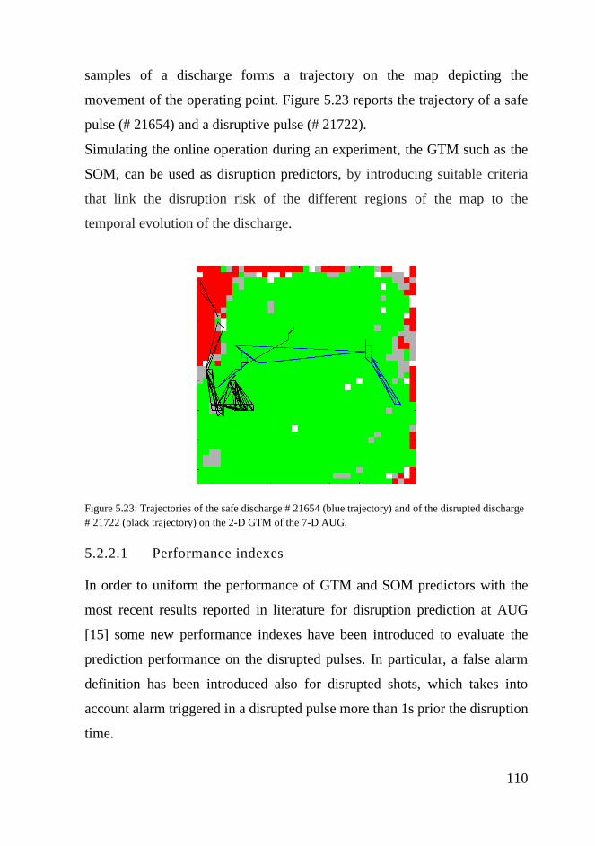
110
samples of a discharge forms a trajectory on the map depicting the
movement of the operating point. Figure 5.23 reports the trajectory of a safe
pulse (# 21654) and a disruptive pulse (# 21722).
Simulating the online operation during an experiment, the GTM such as the
SOM, can be used as disruption predictors, by introducing suitable criteria
that link the disruption risk of the different regions of the map to the
temporal evolution of the discharge.
Figure 5.23: Trajectories of the safe discharge # 21654 (blue trajectory) and of the disrupted discharge
# 21722 (black trajectory) on the 2-D GTM of the 7-D AUG.
5.2.2.1 Performance indexes
In order to uniform the performance of GTM and SOM predictors with the
most recent results reported in literature for disruption prediction at AUG
[15] some new performance indexes have been introduced to evaluate the
prediction performance on the disrupted pulses. In particular, a false alarm
definition has been introduced also for disrupted shots, which takes into
account alarm triggered in a disrupted pulse more than 1s prior the disruption
time.

111
Moreover, the time windows of the alarm trigger for the successful
predictions and the early detections have been redefined, as in the following.
The new performance indexes are defined as follows:
SPs: Successful Predictions, fraction of disruptive discharges which
are correctly predicted. A disruption is correctly predicted if the
predictor is able to trigger the alarm in the time interval [tD-500 ÷ tD-
2] ms. The new lower bound of 500 ms has been adopted following
[15]. Note that this bound is less restrictive with respect to that used
in section 5.1.1.2.
EDs: Early Detections, fraction of disruptive discharges where the
alarm is triggered more than 500 ms but less than 1s before the
disruption time. The time of 1s before the disruption has been
adopted because before this time the disruption precursors are hardly
ever observed [15].
FAD: False Alarms in a disrupted discharge are generated when a
disruption alarm is triggered more than 1s prior the disruption time.
The other performance indexes, SR, TD, MA on disrupted pulses and FA
and SP on safe pulses (reported in the § 5.1.1.2) remain unchanged.
5.2.2.2 Alarm criterion
Due to the good results achieved by the SOM predictors, presented in
chapter 5.1, the same algorithm introduced in section 5.1.1.3 has been used
to trigger the alarm in the GTM and the SOM trained using discharges
performed between 2007 and 2012. In order to reduce the FAs, FADs and the
EDs, a small change in the alarm criteria has been adopted. It consists in the
optimization of the minimum number of the waiting samples (kMIN) when the
trajectory stays in red clusters, which was set equal 2 in section 5.1.1.3.
112
For each disrupted and mixed cluster, the parameter k was evaluated by the
linear relation (5.1):
100%
%%
MIN
MIN
MINMAX
MAX
DS
DSDS
kk
kk
100for % DSDS%MIN (5.3)
Maximizing the SR on Training Set, the parameters DSMIN%, kMAX and kMIN
have been optimized in the range:
DSMIN %=80÷98
kMAX=15÷35
kMIN=2÷10
The value of k is updated only if the trajectory moves into clusters with
higher DS%. Conversely, the alarm is not triggered at all in clusters with
DS%< DS%MIN.
The best performance on Training Set has been obtained by triggering the
alarm when the trajectory stays in red or mixed clusters for at least k
consecutive samples with:
4484.4 % DSk for the GTM with DS%MIN=95%
5555.5 % DSk for the SOM with DS%MIN=98%
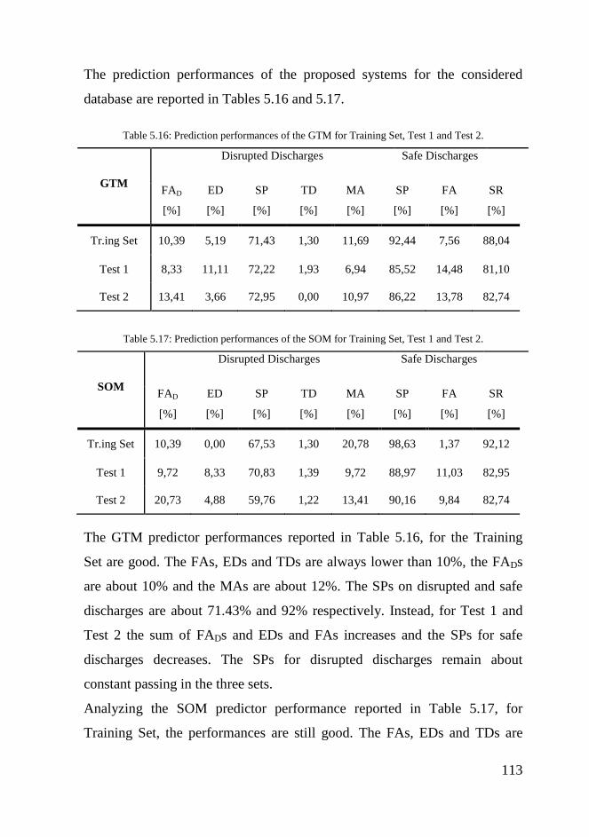
113
The prediction performances of the proposed systems for the considered
database are reported in Tables 5.16 and 5.17.
able 5.16: Prediction performance of the GTM for Training Set, Test 1 and Test 2.
Table 5.16: Prediction performances of the GTM for Training Set, Test 1 and Test 2.
GTM
Disrupted Discharges Safe Discharges
FAD
[%]
ED
[%]
SP
[%]
TD
[%]
MA
[%]
SP
[%]
FA
[%]
SR
[%]
Tr.ing Set 10,39 5,19 71,43 1,30 11,69 92,44 7,56 88,04
Test 1 8,33 11,11 72,22 1,93 6,94 85,52 14,48 81,10
Test 2 13,41 3,66 72,95 0,00 10,97 86,22 13,78 82,74
Table 5.17: Prediction performances of the SOM for Training Set, Test 1 and Test 2.
SOM
Disrupted Discharges Safe Discharges
FAD
[%]
ED
[%]
SP
[%]
TD
[%]
MA
[%]
SP
[%]
FA
[%]
SR
[%]
Tr.ing Set 10,39 0,00 67,53 1,30 20,78 98,63 1,37 92,12
Test 1 9,72 8,33 70,83 1,39 9,72 88,97 11,03 82,95
Test 2 20,73 4,88 59,76 1,22 13,41 90,16 9,84 82,74
The GTM predictor performances reported in Table 5.16, for the Training
Set are good. The FAs, EDs and TDs are always lower than 10%, the FADs
are about 10% and the MAs are about 12%. The SPs on disrupted and safe
discharges are about 71.43% and 92% respectively. Instead, for Test 1 and
Test 2 the sum of FADs and EDs and FAs increases and the SPs for safe
discharges decreases. The SPs for disrupted discharges remain about
constant passing in the three sets.
Analyzing the SOM predictor performance reported in Table 5.17, for
Training Set, the performances are still good. The FAs, EDs and TDs are

114
always lower than 10% and the FADs are about 10%. But the MAs are higher
than 20%. The SPs on disrupted and safe discharges are respectively about
67% and 99%. Instead, for Test 1 and Test 2 the sum of FADs and EDs and
FAs increases and the SPs for disrupted and safe discharges decrease.
The SRs obtained with SOM predictor result to be better than those obtained
with the GTM predictor, for the Training Set and Test 1, but for the Test 2
the SR is the same for both predictors. Moreover, the GTM has always better
performance on MAs and SPs for disrupted discharges, for all datasets,
whereas the SOM achieves lower FAs than the GTM, for all datasets.
Even if the prediction performance for SOM and GTM are quite good, they
are not fully satisfactory (for example, the MAs for SOM for the training set
are greater than 20% or FADs are about 20% for the Test 2). This may be due
to the wrong choice of the tpre-disr during the training phase of the maps. In
this training procedure the tpre-disr has been set equal to 45ms before the tD for
all disrupted discharges, as reported in [39]. Note that, this time instant has
been optimized by the authors by means of a heuristic procedure using data
coming from the experimental campaigns from 2002 to 2005. This time
instant may not be appropriate for the disrupted discharges coming from the
experimental campaigns from 2007 to 2011, which are used to train the
SOM and the GTM. A wrong choice of the tpre-disr gives ambiguous
information to the models in cases of disruptions with disruptive phase
different from 45ms. In fact, during the labeling of the disruptive samples in
the training phase of the models two different problems could arise. The first
one appears if the actual disruptive phase be shorter than 45ms, in this case,
some non-disrupted samples are labeled as disruptive. The second one
appears if the disruptive phase is longer than 45ms, in this case some
disruptive samples are omitted in the training phase and hence the models
are poorer in terms of disruptive knowledge provided.

115
5.2.3 Disruptive phase identification using the Mahalanobis distance
The assessment of a specific disruptive phase for each disruptive discharge
represents a relevant issue in the understanding of disruptive events, but the
identification of the beginning of this phase is often a very difficult task if
physical criteria are used.
In this thesis, the Mahalanobis distance [36] has been applied to define a
specific disruptive phase for each disruption. Mahalanobis distance is used in
literature to detect outliers of a prefixed distribution. An outlier is an
observation that numerically deviates abnormally from other values in the
rest of the population it belongs to. In this thesis an outlier can be seen as a
disruptive sample and the group of reference points is assumed to be the safe
discharges in the training set.
Monitoring the Mahalanobis distance for the disruptive pulses, it was noted
that the Mahalanobis distance is low during the evolution of the discharge
and increases when the disruption is approaching. This suggested us to use
the Mahalanobis distance to select the disruptive samples. Hence, a different
tpre-disr has been selected for each disrupted pulse in the training set by labeling
each sample as safe or disruptive depending on its Mahalanobis distance
value. Therefore, a suitable threshold on Mahalanobis distance, which
discriminates between disruptive and safe configurations, has to be set.
In this thesis the optimization of the Mahalanobis threshold has been carried
out and a confidence limit of about 99% has been empirically assumed for
the Mahalanobis distance of safe points. By means of this threshold (TH) it
is possible to exclude 1% of outliers of the reference points distribution. As
previously mentioned, an outlier can be considered as a disrupted sample.
As an example, Figure 5.24 reports the Mahalanobis distance for a safe
(#21654) and a disruptive (#21722) discharge belonging to the training set.
The green line, on both plots, indicates the threshold TH (TH=1.93). As it

116
can be noted, the Mahalanobis distance remains always well below the
threshold for the safe shot (Figure 5.24(a)), whereas, for the disruptive shot
(Figure 5.24 (b)), the Mahalanobis distance increases when the disruption is
approaching and crosses the threshold (the green line) when t=3.58s.
Figure 5.24: Mahalanobis distance for the safe discharge #21654 (a) and the disruptive discharge
#21722 (b). The green line is the selected threshold (TH).
In Figure 5.25 the distribution of the length of the pre-disrupted phase for the
disrupted pulses of the training set is reported, evaluated using the
Mahalanobis distance.
Figure 5.25: Distribution of the length of the pre-disrupted phase for the disrupted pulses of the
Training Set.

117
As it can be noted, the majority of disrupted pulses in the Training Set has a
disruptive phase length of about 6ms. Besides, there are disrupted pulses
with a disruptive phase longer than 45ms.
Figure 5.26 reports the cumulative distributions of the length of the pre-
disrupted phase for the disrupted pulses in the Training Set. As can be noted,
48% of the pulses has a pre-disruptive phase equal or shorter than 6 ms,
93.5% has a pre-disruptive phase equal or shorter than 52 ms.
Figure 5.26: Cumulative histogram of the length of the pre-disruptive phase for the pulses of the
Training Set.
The resulting number of samples selected as disruptive by means of the
Mahalanobis distance is 2.947 instead of 3.465 samples previously selected
considering all the samples in the last 45ms.
A new GTM and SOM with a disruptive phase selected by means of the
Mahalanobis distance have been trained. The number of clusters in the SOM
and GTM, chosen as previously described, are 1.369 and 1.333 respectively.
For comparison purposes, the composition in terms of cluster types for the
GTM trained with a tpre-disr equal 45 ms before the disruption time tD (GTM1)
and the GTM trained with a tpre-disr|MD selected using the Mahalanobis distance

118
(GTM2) is shown in Table 5.18. Figure 5.27 shows the GTM1 and the
GTM2.
Figure 5. 27:
Figure 5.27: GTM1 trained with tpre-disr equal 45 ms before the disruption time and GTM2 trained with
tpre-disr|MD. Note that the map dimension remains unchanged passing from GTM1 to GTM2.
Table 5.18:
Table 5.18: Cluster composition for GTM1 and GTM2
Cluster type GTM1 [%] GTM2 [%]
Safe 83,20 85,98
Disrupted 8,77 7,30
Mixed 5,99 4,67
Empty 2,05 2,04
Analyzing Table 5.18 it can be noted that, passing from GTM1 to GTM2, a
decrease of the mixed clusters is achieved. The empty clusters for the two
GTMs remain unchanged. The disrupted clusters decrease and the safe
clusters increase. The mixed clusters reduction can be interpreted as a better
discrimination capability of the mapping between safe and disrupted
behaviors.
The GTM composition in terms of samples into the clusters is reported in
Table 5.19. As can be noted, passing from GTM1 to GTM2 a decrease of the
disruptive and mixed samples contained in the disruptive and transition

119
regions respectively, and an increase of the safe samples contained in the
safe region is achieved. This is indicative again of a better discrimination
capability of GTM2 with respect to GTM1.
Table 5.19:
Table 5.19 Clusters composition in terms of total samples for GTM1 and GTM2.
Samples/Total Samples [%]
Safe Disrupted Mixed
GTM1 84,54 8,33 7,71
GTM2 87,60 6,98 5,42
Table 5.20 reports the GTM samples distribution into the clusters. As can be
noted, passing from GTM1 to GTM2 an increase of the disruptive and safe
samples contained in the disruptive and safe regions is achieved. This is
indicative again of a better discrimination capability of GTM2 with respect
to GTM1.
Table 5.20: Cluster composition in terms of safe and disrupted samples for GTM1 and GTM2.
Cluster
GTM1 GTM2
Safe samples/
Total safe
samples [%]
Disruptive
samples/Total
Disruptive
samples [%]
Safe samples/
Total safe
samples [%]
Disruptive
samples/Total
Disruptive
samples [%]
Safe 95,45 --- 97,28% ---
Disrupted --- 70,13 --- 72,88
Mixed 4,55 29,87 2,72% 27,12
The SOM composition in terms of cluster type for SOM trained with a tpre-disr
equal 45 ms before the disruption time, tD (SOM1) and the SOM trained with
a tpre-disr|MD selected using the Mahalanobis distance (SOM2) is shown in Table
5.21. Figure 5.28 shows the SOM1 and the SOM2.

120
Figure 5.28: SOM1(with 1364 cluster) trained with a tpre-disr equal 45 ms before the disruption time and
SOM2 (with 1333 cluster) trained with a tpre-disr|MD.
Analyzing Table 5.21 it results that, passing from SOM1 to SOM2 a
decrease of the mixed clusters is achieved. The empty clusters for SOM
remain about unchanged. The mixed clusters reduction can be interpreted as
a better discrimination capability of the mapping between safe and disrupted
behaviors.
Table 5.21:
Table 5.21: Cluster composition for SOM1 and SOM2.
Cluster type SOM1 [%] SOM2 [%]
Safe 81,89 84,85
Disrupted 8,34 7,88
Mixed 7,64 5,25
Empty 2,13 2,02
The SOM composition in terms of samples into the clusters is reported in
Table 5.22. Passing from SOM1 to SOM2 a decrease of the mixed samples
contained in the transition region is shown, whereas an increase of the safe
samples contained in the safe region is achieved. The disruptive samples
contained in the disruptive region remain about constants.

121
Table 5.22:
Table 5.22: Clusters composition in terms of total samples for SOM1 and SOM2.
Samples/Total samples [%]
Safe Disrupted Mixed
SOM1 80,88 6,74 12,38
SOM2 86,12 6,80 7,08
The Table 5.23 reports the SOM samples distribution into the clusters.
Passing from SOM1 to SOM2 an increase of the disruptive and safe samples
contained in the disruptive and safe regions respectively, is achieved. This is
indicative again of a better discrimination capability of SOM2 with respect
to SOM1.
Table 5.23: Cluster composition in terms of safe and disrupted samples for SOM1 and SOM2.
Cluster
SOM1 SOM2
Safe samples/
Total safe samples [%]
Disruptive
samples/ Total
disruptive
samples [%]
Safe samples/
Total safe
samples [%]
Disruptive
samples/ Total
disruptive
samples [%]
Safe 91,40 --- 95,64 ---
Disrupted --- 58,59 --- 68,27
Mixed 8,60 41,41 4,36 31,73
In order to prove that the wrong choice of the tpre-disr could influence the
prediction performance, they have been evaluated for GTM2 and SOM2
predictors. For comparison purposes, the prediction performances for GTM1
and SOM1 are reported again.
The same alarm criterion presented in the § 5.2.2.2, for both predictors, is
adopted.
Table 5.24 reports the prediction performances for GTM2 while Table 5.25
reports prediction performances for GTM1. The best performances on
Training Set, for GTM2, are achieved activating the alarm when the
trajectory stays in red or mixed cluster for at least k consecutive samples:

122
2052 % DSk with DS%MIN=95%. These coefficients were optimized
maximizing the SR on the training set.
Table 5.24:
Table 5.24: Prediction performances for GTM2.
GTM 2 Disrupted Discharges Safe Discharges
FAD
[%]
ED
[%]
SP
[%]
TD
[%]
MA
[%]
SP
[%]
FA
[%]
SR
[%]
Tr.ing Set 5,19 5,19 77,92 3,90 7,79 96,91 3,09 92,93
Test 1 8,33 6,94 75,00 1,39 8,33 88,97 11,03 84,33
Test 2 12,20 2,44 73,16 0,00 12,20 89,76 10,24 85,71
Table 5.25: Prediction performances for GTM1.
GTM 1 Disrupted Discharges Safe Discharges
FAD
[%]
ED
[%]
SP
[%]
TD
[%]
MA
[%]
SP
[%]
FA
[%]
SR
[%]
Tr.ing Set 10,39 5,19 71,43 1,30 11,69 92,44 7,56 88,04
Test 1 8,33 11,11 72,22 1,93 6,94 85,52 14,48 81,10
Test 2 13,41 3,66 72,95 0 10,97 86,22 13,78 82,74
Comparing Tables 5.24 and 5.25 it can be noted that using a different tpre-disr
for each disrupted discharges leads to an increase of the performances of the
GTM predictor. In particular, the global success rates SRs and the SPs for
safe and disrupted discharges increase for all datasets. The FADs, the EDs
and the FAs decrease for all dataset. Note that, a slight increase of the MAs
for Test Set 1 and 2 is achieved.
Table 5.26 reports the prediction performances for the SOM2 while Table
5.27 reports the prediction performances for the SOM1. The best
performances on Training Set, for SOM2, are achieved activating the alarm
when the trajectory stays in red or mixed cluster for at least k consecutive

123
samples: 5025 % DSk with DS%MIN=98%. These values were
optimized maximizing the SR on the training set.
Table 5.26: Prediction performances for SOM2.
SOM2 Disrupted Discharges Safe Discharges
FAD
[%]
ED
[%]
SP
[%]
TD
[%]
MA
[%]
SP
[%]
FA
[%]
SR
[%]
Tr.ing Set 6,49 3,90 77,92 1,30 10,39 94,85 5,15 90,76
Test 1 8,33 6,94 72,22 2,78 9,72 89,66 10,34 83,87
Test 2 9,76 3,66 76,83 0,00 9,76 90,55 9,45 87,20
Table 5.27: Prediction performances for SOM1.
SOM1 Disrupted Discharges Safe Discharges
FAD
[%]
ED
[%]
SP
[%]
TD
[%]
MA
[%]
SP
[%]
FA
[%]
SR
[%]
Tr.ing Set 10,39 0,00 67,53 1,30 20,78 98,63 1,37 92,12
Test 1 9,72 8,33 70,83 1,39 9,72 88,97 11,03 82,95
Test 2 20,73 4,88 59,76 1,22 13,41 90,16 9,84 82,74
Comparing Tables 5.26 and 5.27 it can be noted that using a different tpre-disr
for each disrupted discharges leads to an increase of the performances of the
predictor. In particular, the global success rates SRs and the SPs for safe and
disrupted discharges increase for all datasets (except for SPs for the safe
discharges in the Training Set). The FADs, the EDs and the FAs decrease for
all datasets.
It is interesting to note that the successful prediction for the disrupted
discharges for GTM2 and SOM2 remain high for all data sets, suggesting
that the ageing phenomenon is not present. Further analyses have been
developed in chapter 6 to justify that.

124
5.2.4 Disruption prediction using the Logistic Regression
The logistic regression is a well-known statistic method to analyze problems
with dichotomous (binary) dependent variables. It models the probability of
a case being classified into one category of the dependent variable as
opposed to the other, using D independent variables or predictors. In this
thesis a Logit Model has been trained to predict the probability that a generic
sample belongs to a safe or a disruptive phase and the independent variables
are the plasma parameters.
Data for this study were extracted from the AUG experimental campaigns
performed between May 2007 and November 2012. The database
composition is reported in Table 5.15.
During the training of the model, the dichotomous output has been set equal
to 0 for safe samples and 1 for disruptive samples. Safe samples come from a
reduced representative set of samples belonging to safe shots (see section
5.2.1.1). The disruptive samples come from a time window of disrupted
shots identified through the Mahalanobis distance criterion (see section
5.2.4).
The plasma parameters used to train the Logit Model are the same seven
plasma parameters used to build the GTM and the SOM predictors presented
in section 5.2.2. The Logit Model inputs are normalized in the interval [0,1].
In this way, the Logit Model Output (LMO) does not depend on the absolute
magnitude of the signals.
The Logit Model is built according to equation 4.11. Taking into account 7
plasma parameters as inputs, the equation 4.11 becomes as in the following:
)(. 76
5432951
GWLfindLM
liPPqLMO pradinp
(5.4)

125
where the parameters α and β are the LMO coefficients estimated during the
training by minimizing the misclassifications via Maximum-Likelihood
method.
It has been observed that for the majority of safe discharges belonging to the
training set, the LMO is always smaller than 0 throughout the discharge. On
the contrary, for the great majority of the disrupted discharges, the time
evolution of the LMO remains at low values during the first part of the
discharge and starts to grow when the pulse approaches the disruption time.
As an example, Figure 5.29 reports the LMO for a safe (#21654) and a
disruptive (#21722) discharge.
Figure 5.29: Logit Model Output (LMO) for a safe discharge #21654 and a disruptive discharge
#21722 (lower plot).
This behavior suggests using the Logit Model as disruption predictor by
introducing a threshold value able to properly identify an incoming
disruption.
Figure 5.30 reports the probability density function (pdf) of the LMO for
samples belonging to the safe and disruptive discharges of the Training Set.
As it can be noted, the distribution of safe samples belonging to safe shots
(in blue) and those belonging to the safe samples of disruptive shots in the
interval [tflat-top ÷ tpre-disr|MD] (in green) are well separated from that of

126
disruptive sample (in red). Therefore, a suitable threshold on the LMO value
can be set to discriminate between safe and disruptive phase of the pulse. A
disruption alarm can be triggered when the LMO exceeds the threshold
value. Moreover, to avoid false alarms sometimes caused by spikes in the
diagnostic signals, a time delay has been introduced that inhibits the alarm
for k samples after the alarm activation.
The optimum LMO threshold has been optimized in the range (0÷5) where
the pdfs of safe and disruptive samples have a limited overlap and the
parameter k has been optimized in the range (1÷10).
Figure 5.30: Probability density function of the LMO for samples belonging to the training set.
The best performance of the LMO as disruption predictor has been achieved
with an alarm threshold equal to 3.9 and k =1 (see Table 5.24). These values
have been optimized maximizing the SR on the Training Set.

127
Table 5.28: Prediction performance for the Logit predictor on the three data sets.
Data set
Disrupted Discharges Safe Discharges
FAD
[%]
ED
[%]
SP
[%]
TD
[%]
MA
[%]
SP
[%]
FA
[%]
SR
[%]
Tr.ing 0,00 0,00 94,81 3,90 1,30 98,63 1,37 97,83
Test 1 2,78 0,00 91,67 2,78 2,78 97,24 2,76 95,39
Test 2 2,44 3,66 92,68 0,00 1,22 95,28 4,72 94,64
Analyzing the Logit predictor performances reported in Table 5.24, for
Training Set, the performances are very high. The FADs, FAs, EDs and TDs
are always lower than 4%. Moreover the FADs and EDs are nulls. The SPs
on disrupted and safe discharges are about 95% and 99% respectively.
The prediction performances remain high both for Test 1 and Test 2. The
FADs, FAs, EDs and TDs are always lower than 5%. The global success
rates SRs are always greater than 94% for all data sets.
The prediction performance of the Logit predictor are better than those of the
GTM2 and SOM2 predictors, furthermore they remain quite high for all data
sets.
5.2.5 Conclusions
Data for the second part of this thesis have been selected from experimental
campaigns performed at AUG between May 2007 and November 2012.
The mapping of the AUG operational space has been proposed using seven
plasma parameters by means the Self Organizing Maps and the Generative
Topographic Mapping.
The maps are trained using a reduced set of samples coming from the safe
discharges and the samples in the last 45ms of the disrupted discharges as
disrupted samples.

128
The maps (GTM1 and SOM1) have been used as disruption predictors by
analyzing the trajectories described over the map by the discharges under
test. The performance has been evaluated using the data coming from
experimental campaigns different from those used to build the maps. The
prediction performances of the predictors are good. For the GTM1 predictor
the SPs on disrupted and safe discharges are about 71.43% and 92%
respectively and decreases of few percentage points passing from Training
Set to Test 1 and Test 2. The global success rate SR is always greater than
81% for all dataset. For the SOM1 predictor the SPs on disrupted and safe
discharges are about 68% and 98% respectively and decreases of few
percentage points passing from Training Set to Test 1 and Test 2. The global
success rate SR is always greater than 88% for all dataset but the MAs are
greater than 20% for the Training Set.
In order to improve the prediction performance of the previous predictors, a
different selection of the disruptive samples using the Mahalanobis distance
has been performed and the SOM and GTM predictors has been re-trained
(GTM2 and SOM2). From a detailed analysis of the map compositions it
resulted that using the Mahalanobis distance to select the disruptive samples
gives mappings (GTM2 and SOM2) with a discrimination capability
between safe and disruptive behaviors better than the maps GTM1 and
SOM1. In fact a reduction of the mixed clusters and the samples inside them
is achieved.
Furthermore, the new training session has led an improvement of the
prediction performances.
For both Test 1 and Test 2 the performances increase passing from GTM1 to
GTM2 and from SOM1 to SOM2.

129
For GTM2 the global success rate on both the test sets is good, always
higher than 84%. In particular, the success predictions are good both on
disrupted and safe shots.
For SOM2 the global success rate on both the test sets is good, always higher
than 83%. In particular, the success predictions are good both on disrupted
and safe shots.
Finally, a logistic regressor has been proposed as disruption predictor. The
Logit Model built with seven plasma parameters as inputs is able to model
the probability that a generic sample belongs to a non-disruptive or a
disruptive phase of the discharges and introducing a suitable alarm criteria it
has been used to identify an incoming disruption.
The prediction performance of the proposed system is very encouraging. The
FADs, EDs and FAs are always lower than 4% and the global success rate is
always greater than 94% for all 3 data sets.
Even if the prediction performances of the Logit Model are better than those
of GTM2 and SOM2, it is not suitable to describe the operational space of
the machine. The GTM, such as the SOM, could be useful in the
identification of the boundaries of the disruption free plasma parameters
space leading to an increase in the knowledge of disruptions.

130
6 DISRUPTION CLASSIFICATION AT
ASDEX UPGRADE
Avoidance or mitigation of disruptions is of primary importance in order to
preserve the integrity of tokamak machines. In this frames, it would be
helpful to distinguish the cause of the disruption, because different
disruption classes may require different avoidance and mitigation strategies.
The avoidance strategies are focused in preventing that the plasma enters in
regions of the operational space with high risk of disruption by either
suppressing or keeping under control instabilities or precursors whose
growth typically leads to disruption. If avoidance fails the unique action that
can be taken is to mitigate the consequences of the disruption by means, e.g.,
of the injection of a large amounts of gas.
Nevertheless, different disruption types could have also an implication on
the effect of the mitigation: for example, it has been proven in JET that,
depending on the underlying conditions, the killer gas injection has not
always the same positive effect. Therefore, being different disruption types
interested by different regions of the operational space, it would be
particularly useful to investigate on possible dependencies with respect to the
different effects of the mitigation, to understand whether this depends on the
disruption type, the disruption phase, or some other mechanism.
Therefore, the need to develop reliable prediction of the disruption type is
essential in order to optimize the strategy to safely land the plasma and to
reduce the probability of damages of the device [6].
In literature some contributions have been devoted to the disruptions
classification. Moreover, a considerable effort is dedicated to understand the
physics of disruptions with the aim to find the root causes of the
phenomenon, therefore a strong interest in developing methods and

131
techniques to manually and automatically classify disruptions is taking place
in the last years. In [5] a manual classification is proposed for the discharges
occurring during the JET operations with the Carbon Wall (JET-C) from
2000 to 2010, while in [11] a manual classification is proposed for the
discharges occurring during the JET operations with the ITER like Wall
(JET-ILW) from 2011 to 2012. In both the papers the specific chain of
events that led to a disruption was identified and used to classify disruptions,
grouping those that follow specific paths. Sometimes these paths are clear
and unique, while others could follow near similar courses. Moreover,
several different physics phenomena may occur simultaneously, eventually
leading to a disruption. This means that not always an unambiguous manual
classification is possible [5]. In [12] the authors proposed a manual
classification for the disruptions occurred at AUG in 2013 (part of the 2012-
2013 experimental campaign). Disruptions with similar causes were
categorized, when possible, according to the classification used for JET in
[11].
Instead, in [6] the disruptions manually classified in [5] were automatically
classified using nonlinear manifold learning methods.

132
6.1 Manual classification at AUG
In this work three disruption predictors have been designed on a database
containing discharges performed at AUG from May 2007 to November 2012
(presented in chapter 5.2). Their performances are evaluated through three
datasets (Training Set, Test 1 and Test 2), and the analysis of the
performance highlights:
o an high generalization capability when the performances are
evaluated using discharges contained in the same time period of the
Training set (Test 1).
o a very low ageing effect when the performances are evaluated using
discharges belonging on later campaigns (Test 2).
The ageing effect is an intrinsic drawback of the data-based models, it
consists in the performance degradation when the model is used with data
temporally far from those used in the training phase; the more the data
temporarily deviate from the training set the higher the performance
degradation is. The ageing effect is very common in the experimental
machines, such as AUG, which operate in ever-changing conditions in order
to explore their potentialities. Therefore, significant ageing was expected on
Test 2.
The high generalization capability and a low ageing effect of the predictors
could be justified if plasma configurations contained in the Training Set are
well representative of those in Test 1 and Test 2.
Hence, a manual classification of the 231 disruptive discharges belonging to
the considered data base has been performed with the aim of examining the
distribution of the disruption classes throughout the three datasets.
The manual classification has been performed by means of a visual analysis
of several plasma parameters for each disruption and taking also into account
the aim of the different experiments. The manual classification criteria try to

133
follow that performed in [5]. In particular, the specific chains of events have
been detected and used to classify disruptions and when possible, the same
classes introduced for JET are adopted [5].
The analysis of physical and technical mechanisms that lead to a disruption
allowed us to identify 9 disruption classes and these classes are reported in
Table 6.1.
Table 6.1: AUG disruption classes and their acronyms.
Disruption Class Acronym
1 H-mode Greenwald Limit GWL-H
2 L-mode Greenwald Limit and density
control problem NC
3 Impurity control problem IMC
4 Auxiliary power shut down ASD
5
CE (disruption characterized by the
radiative collapse and current profile
peaking)
CE
6 Impurity accumulation (radiation peaking) RPK
7 β-limit disruption β-limit
8 Low-q and low-ne or Error field
disruption LON-EFM
9 Vertical displacement event VDE
Disruptions clustered in the first five classes are typically characterized by
the final cooling of the edge and differ mainly for the root cause of the chain
of events. As already explained in chapter 2 (§2.3), the cooling of the plasma
edge (CE) can be summarized with the following chains of phenomena: the
radiation losses exceeds the heating power, then the temperature collapses
causing the contraction of the plasma current profile, resulting in an
increasing of the internal inductance [5,14, 15]. The cooling of the plasma
edge makes the plasma unstable to MHD tearing modes, which leads to

134
disruption. As shown in the section 2.3, the cooling of the plasma edge can
be achieved in two different ways: by means of a high level of electron
density or by means of a high impurity density at the edge.
The first one can be achieved by a continuous gas puffing, which leads to a
saturation of the density increase with a following energy collapse and a
disruptive termination of the discharge [19]. This phenomenology can be
detected in the CE due to achieved Greenwald limit after H/L back transition
and in the CE due to achieved Greenwald limit in L-mode discharge.
In addition to physical causes, the diagnostic problems could be another
cause of disruptions characterized by a cold edge. For example, an erroneous
density signal due to a fringe-jump of the interferometer signal may lead to
excessive gas requests from the density feedback system pushing again the
plasma towards the density limit. This happens in the CE due to density
control problem. When the plasma operates near to the Greenwald limit the
H-L back transition may occur as consequence of a sudden drop of the input
power related to an auxiliary power system switch-off, usually the NBI. The
fast switch-off of auxiliary power could lead to difficulties in controlling
density leading to the discharge disruption [5]. This happens in the CE due to
auxiliary power shut-down.
The second one is directly linked to a power balance problem at the edge. If
the edge cools to a sufficiently low temperature, a radiative instability can
occur due to the effect of a small concentration of impurities (typically low-
Z impurities released from the first wall or deliberately introduced) that
changes the plasma radiation characteristics in such a way that, with
decreasing temperature, an increasing radiative loss occurs [19]. This
happens in the CE due to impurity control problem.
Another important cause of instability related to plasma radiation is the
impurity accumulation of high-Z materials in the plasma centre due to

135
plasma wall interactions (mostly Tungsten in the considered database). This
accumulation gives rise to strong core radiation due to the fact that high-Z
impurity atoms are able to reach the centre without being fully ionized. This
leads to a flattening or even a hollowing of the current density due to an
increase of the plasma resistivity. If this mechanism is amplified, the central
temperature collapses, then the plasma ends in a disruption due to the onset
of MHD activity.
Regarding the MHD stability, one restriction on the accessible operational
domain is imposed by the Troyon ideal MHD limit. The Troyon limit defines
the maximum plasma pressure which can be confined for a given toroidal
magnetic field, typically expressed with a limit on the volume averaged
toroidal β. High β plasmas are unstable to external kink modes, and,
depending on the boundary conditions, are mainly restricted by Neoclassical
Tearing Modes (NTMs) and Resistive Wall Modes (RWMs).
MHD instabilities, such as locked modes, could be excited by error fields,
which are deviations of the magnetic fields from axisymmetry. In AUG the
error fields are not particularly significant, but studies of error fields have
been carried out in the last 2 years by means of the Resonance Magnetic
Perturbation coils (RMP), which generate a n=1 radial magnetic field
resonant on the surface q=2, in low density and low q95 plasmas [12].
For some pulses, disrupted by means a radiative collapse, most of the plasma
signals required for the classification were not available. These disruptions
have been grouped in a class labeled Other.
Moreover, during the disruptions database analysis it has been observed that
various disruptions arose through a mechanism not matching with those
described above (cooling edge, radiation peaking, LON-EFM). For some of
them, the performed analysis has shown only to the presence of a mode that
grows and finally locks. Thus, a further class, called “MOD”, has been

136
defined, where the common phenomenon leading to the disruption is only
the locked mode.
Finally, when the plasma cross section is elongated, as at AUG, the plasma
column is inherently unstable to the motion in the direction of elongation. A
fast change in plasma parameters can cause the loss of the vertical position
control, leading the plasma column to contact the first wall reducing the
safety factor at the edge. When the edge safety factor decreases to a
sufficiently low value, rapid growth of MHD activity produces a fast thermal
quench similar to those observed in major disruptions. The vertical
displacement events (VDEs) are excluded from the database used for the
classification, because they are easily predictable at AUG monitoring the
deviation of the vertical position of the plasma centroid with respect to the
feedback reference position [15].
In the following, for each class, an example of its evolution is reported and
commented.

137
6.1.1 Example of NC disruption
An example of a disruption due to the achieving of density limit in a
classical L-mode density limit discharge (NC) is reported in Figure 6.1. The
figure reports the temporal evolution of: (a) the plasma current [MA], (b) the
line average density in the plasma core [1019
m-2
], (c) the Greenwald fraction
[a.u], (d) the total input power [MW] together with the total radiated power
[MW], (e) the internal inductance [a.u], (f) the plasma energy [MJ], (g) the
Deuterium gas rate [1020
/s] and (h) the Locked Mode signal [V] for the shot
# 26511.
Figure 6.1: Example of NC disruption (discharge # 26511). (a) Plasma current, (b) line average density
in the core, (c) Greenwald fraction, (d) total input power (blue line) and total radiate power (red line),
(e) internal inductance, (f) plasma energy, (g) Deuterium gas rate, (h) Locked Mode signal. The
disruption time is 1.631s.
In the L-mode configuration, from t=1.538s a continuous gas puffing leads
to a rapid increase of both the line averaged density in the plasma and the
Greenwald fraction, as can be observed in subplot (g), (b) and (c) of Figure

138
6.1; at the same time instant the cooling of the plasma edge takes place
causing the decrease of the plasma energy (Figure 6.1 (d), (e) and (f)
respectively) which deteriorates the plasma confinement. Moreover, at
t=1.587s a mode starts to lock when the Greenwald fraction is equal to 0.87
whereupon the plasma density continues to increase bringing up the
Greenwald fraction values up to 1, then at t=1.631s the discharge ends in a
disruption. During this last phase, a MARFE developed around the X-point
region.
The MARFE can be detected by means of an increasing of the edge density
at the High Field Side with a corresponding increase of the radiation that
could extend also to the X-point region.
Figure 6.2 shows the temporal evolution of the ratio between the line
average density at the edge and the line average density at the core for the
pulse #26511. After 1.6s the increase of such ratio, due to the likely
development of a MARFE, can be clearly observed.
Figure 6.2: Temporal evolution of the ratio between the edge line average density and the core line
average density in pulse # 26511.
Whereas, Figure 6.3 shows the radiated power recorded from the 46
channels of the FHC camera of the bolometer during the last 31ms of the
same discharge. An increase of the radiated power (yellow and red regions)

139
is detectable in the last ~10 ms around the X-point region (covered by the
channels 10-15) highlighting the development of a MARFE.
Figure 6.3: Contour map of the radiated power measured from the 46 channels of the FHC bolometer
camera for the last 31 ms of the pulse #26511. The yellow and red region highlight the development of
MARFE around the X-point region.
6.1.2 Example of GWL-H disruption
An example of a cooling edge disruption due to the achieving of density
limit in a classical H-mode density limit discharge (GWL-H) is reported in
Figure 6.4. The figure reports the temporal evolution of: (a) the plasma
current [MA], (b) the line average density in the plasma core [1019
m-2
], (c)
the total input power [MW] together with the total radiated power [MW], (d)
the Greenwald fraction [a.u], (e) the internal inductance [a.u], (f) the plasma
energy [MJ], (g) the Deuterium gas rate [1020
/s] and (h) the Locked Mode
signal [V] for the shot #26692.

140
Figure 6.4: Example of GWL_H disruption (discharge # 26694). (a) Plasma current, (b) line average
density in the core, (c) total input power (blue line) and total radiate power (red line), (d) Greenwald
fraction, (e) internal inductance, (f) plasma energy, (g) Deuterium gas rate, (h) Locked Mode signal.
The disruption time is 4.654s.
During the H-mode configuration, from t=1s to t=4.172 s the continuous gas
puffing (Figure 6.4(g)) leads to the saturation of the density (Figure 6.4 (b)).
At t=4.172s the Greenwald fraction reaches 0.97 causing an H-L back
transition, resulting in an increase of the density and in a faster decrease of
the plasma energy, as shown in subplots (b) and (f) respectively. At t=4.471s
the cooling of the plasma edge takes place causing a rapid deterioration of
the plasma energy (Figure 6.4 (c), (e) and (f) respectively). Moreover, at
t=4.650s a mode starts to lock, then the discharge ends in a disruption at
t=4.654s.
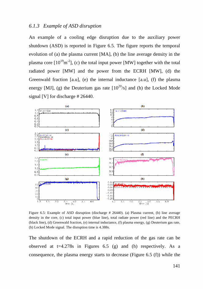
141
6.1.3 Example of ASD disruption
An example of a cooling edge disruption due to the auxiliary power
shutdown (ASD) is reported in Figure 6.5. The figure reports the temporal
evolution of (a) the plasma current [MA], (b) the line average density in the
plasma core [1019
m-2
], (c) the total input power [MW] together with the total
radiated power [MW] and the power from the ECRH [MW], (d) the
Greenwald fraction [a.u], (e) the internal inductance [a.u], (f) the plasma
energy [MJ], (g) the Deuterium gas rate [1020
/s] and (h) the Locked Mode
signal [V] for discharge # 26440.
Figure 6.5: Example of ASD disruption (discharge # 26440). (a) Plasma current, (b) line average
density in the core, (c) total input power (blue line), total radiate power (red line) and the PECRH
(black line), (d) Greenwald fraction, (e) internal inductance, (f) plasma energy, (g) Deuterium gas rate,
(h) Locked Mode signal. The disruption time is 4.388s.
The shutdown of the ECRH and a rapid reduction of the gas rate can be
observed at t=4.278s in Figures 6.5 (g) and (h) respectively. As a
consequence, the plasma energy starts to decrease (Figure 6.5 (f)) while the
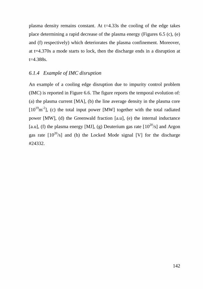
142
plasma density remains constant. At t=4.33s the cooling of the edge takes
place determining a rapid decrease of the plasma energy (Figures 6.5 (c), (e)
and (f) respectively) which deteriorates the plasma confinement. Moreover,
at t=4.370s a mode starts to lock, then the discharge ends in a disruption at
t=4.388s.
6.1.4 Example of IMC disruption
An example of a cooling edge disruption due to impurity control problem
(IMC) is reported in Figure 6.6. The figure reports the temporal evolution of:
(a) the plasma current [MA], (b) the line average density in the plasma core
[1019
m-2
], (c) the total input power [MW] together with the total radiated
power [MW], (d) the Greenwald fraction [a.u], (e) the internal inductance
[a.u], (f) the plasma energy [MJ], (g) Deuterium gas rate [1020
/s] and Argon
gas rate [1020
/s] and (h) the Locked Mode signal [V] for the discharge
#24332.
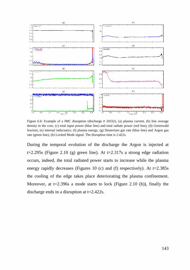
143
Figure 6.6: Example of a IMC disruption (discharge # 24332), (a) plasma current, (b) line average
density in the core, (c) total input power (blue line) and total radiate power (red line), (d) Greenwald
fraction, (e) internal inductance, (f) plasma energy, (g) Deuterium gas rate (blue line) and Argon gas
rate (green line), (h) Locked Mode signal. The disruption time is 2.422s.
During the temporal evolution of the discharge the Argon is injected at
t=2.295s (Figure 2.10 (g) green line). At t=2.317s a strong edge radiation
occurs, indeed, the total radiated power starts to increase while the plasma
energy rapidly decreases (Figures 10 (c) and (f) respectively). At t=2.385s
the cooling of the edge takes place deteriorating the plasma confinement.
Moreover, at t=2.396s a mode starts to lock (Figure 2.10 (h)), finally the
discharge ends in a disruption at t=2.422s.

144
6.1.5 Example of RPK disruption
An example of impurity accumulation disruption (RPK) is reported in
Figure 6.7. The figure reports the temporal evolution of: (a) the plasma
current [MA], (b) the internal inductance [a.u], (c) the tungsten concentration
[nW/ne], (d) the plasma temperature (several channels from ECE diagnostic)
[keV], (e) the plasma energy [MJ], (f) the core and the edge radiation factor
[a.u], (g) the radiation peaking factor [a.u], defined as the radiated power
from the core divided by the radiated power from the edge, and (h) the
Locked Mode signal [V] for the discharge #28172.
Figure 6.7: Example of a impurity accumulation disruption (discharge #28172), (a) plasma current, (b)
internal inductance, (c) W concentration, (d) central temperature (ECE diagnostic), (e) plasma energy,
(f) core and edge radiation, (g) radiation peaking factor (core radiated power/edge radiated power), (h)
Locked Mode signal. The disruption time is t=3.577s.
At t=2.956s the W concentration starts to increase (see Figure 6.7(c)) giving
rise to a strong core radiation as highlighted by both the rising of the cyan
line in Figure 6.7(f) and the growth of radiation peaking factor (Figure
6.7(g)). The strong core radiation leads to the reduction of both the central

145
temperature (Figure 6.7(d)) and the plasma energy (Figure 6.7(e)). At
t=3.120s the core radiation exceeds the edge radiation (Figure 6.7(f))
determining an increase of the radiation peaking factor above one, and a
lowering of the internal inductance (Figure 6.7(g)). Finally a Locked Mode
leads the discharge to a disruption.

146
6.1.6 Example of -limit disruption
An example of ideal -limit disruption is reported in Figure 6.8. The figure
reports the temporal evolution of: (a) the plasma current [MA], (b) the total
input power [MW] together with total radiated power [MA], (c) the line
average density in the plasma core [1019
m-2
], (d) the internal inductance
[a.u], (e) the plasma energy [MJ], (f) the N [a.u], (g) the plasma temperature
(several channels from ECE diagnostic) [keV], (h) the time derivative of the
radial component of B [V/s] and (i) the Locked Mode signal [V] for the
discharge #25175.
Figure 6.8: Example of a -limit disruption (discharge #25175), (a) plasma current, (b) total input
power (blue line) with together the total radiate power (red line), (c) line average density in the core,
(d) internal inductance, (e) plasma energy, (f) N, (g) central temperature (several channels from ECE
diagnostic), (h) time derivative of the radial component of B and (i) Locked Mode signal. The
disruption time is 1.320s.
Ideal -limit disruptions are typically obtained in short experiments in which
the heating power (Figure 6.8 (b)) is sufficient to produce a continuous rise

147
of N, the plasma energy, the electron density and the temperature (Figures
6.8(f), (e), (c) and (g) respectively). A strong MHD instability (visible in
Figure 6.8 (h)) arises at t=1.30s and grows up until t=1.318s when it locks
(Figure 6.8 (i)) terminating the discharge in a disruption at t=1.320s.

148
6.1.7 Example of LON-EFM disruption
In Figure 6.9 a temporary evolution of a LON-EFM disruption is reported
for discharge #26405. The figure reports the temporal evolution of: (a) the
plasma current [MA], (b) the total input power [MW] together with the total
radiated power [MW], (c) the current of the RMP coil [kA], (d) the line
average density in the plasma core [1019
m-2
], (e) the internal inductance
[a.u], (f) the plasma energy [MJ], (g) the absolute value of q95 [a.u], (h) the
plasma temperature (several channels from ECE diagnostic) [keV] and (i)
the time derivative of the radial component of B [V/s].
Figure 6.9:
Figure 6.9: Example of a LON-EFM disruption (discharge #26405). (a) plasma current, (b) total input
power (blue line) with together the total radiate power (red line), (c) the current of the RMP coil, (d)
line average density in the core, (e) internal inductance, (f) plasma energy, (g) |q95|, (h) time derivative
of the B radial component. The disruption time is t=3.751s.

149
As shown in Figure 6.9, a typical LON-EFM disruption is characterized by
very low plasma density, about 1.91019
m-2
(Figure 6.9(d)), together with a
very low value of |q95|, slightly above 3 (Figure 6.9(g)). In this configuration
the RMP current starts to increase at t=1.85s (Figure 6.9(c)). At t=3.751s the
confinement is deteriorated due to a strong MHD activity detected by the
Mirnov coils (Figure 6.9 (h)), which results in the final drop of the plasma
energy (Figures 6.9 (f)).

150
6.1.8 Example of a MOD disruption
In Figure 6.10 a temporary evolution of a MOD disruption is reported for
discharge #26315. The figure reports the temporal evolution of the last
500ms of: (a) the plasma current [MA], (b) the total input power [MW]
together with the total radiated power [MW], (c) the line average density in
the plasma core [1019
m-2
], (d) the internal inductance [a.u], (e) the plasma
energy [MJ], (f) the N [a.u], (g) the plasma temperature (several channels
from ECE diagnostic) [keV], (h) the Locked Mode signal [V] and (i) the
time derivative of the radial component of B [V/s].
Figure 6.10: Example of a MOD disruption (discharge #26315), (a) plasma current, (b) total input
power (blue line) together with the total radiated power (red line), (c) line average density in the
plasma core, (d) internal inductance, (e) plasma energy, (f) N, (g) plasma temperature (several
channels from ECE diagnostic) [keV], (h) Locked Mode signal and (i) time derivative of the radial
component of B. The disruption time is t=3.406s.

151
As shown in Figure 6.10, the only phenomenon that can be observed in a
MOD disruption is the strong MHD activity and then the final locked mode
that leads a disruption the discharge.
During the normal evolution of the discharge #26315, a strong MHD
instability (visible in Figure 6.10 (i)) arises and grows at t=3.364s, then it
locks in t=3.394s (Figure 6.10 (h)) terminating the discharge in a disruption
at t=3.406s.

152
6.2 Statistical analysis of the manual classification at
AUG
Following the chain of events that leads to each disruption outlined in the
previous paragraphs, described by means of the time evolution of several
plasma parameters, the 231 disruptions have been manually classified. The
manual classification consists in associating a label to each disruption of the
Training Set, Test 1 and Test 2. The database composition of the disrupted
discharges is shown in Table 6.2.
Table 6.2:
Table 6.2: Disruption database composition
Data set Disrupted pulses Time Period
Training Set 77 May 2007- April 2011
Test 1 72 May 2007- April 2011
Test 2 82 May 2011- April 2012
Note that, as previously mentioned, the VDEs are excluded from the
database and for this reason they are not present in the following statistics.
The percentage frequency of occurrence of each disruption class (Disruption
Class Rate, DCR) for each data set is computed with respect to the total
number of disrupted discharges belonging to the considered data set.
The histograms in Figures 6.10-6.12 show the Disruption Class Rate versus
the disruption classes for each data set.

153
Figure 6.11: Disruption Class Rate % versus the disruption classes for the Training Set.
Figure 6.12: Disruption Class Rate % versus the disruption classes for the Test 1.
ASDGWL-
HIMC CE NC
LON-
EFMβ-limit RPK MOD Other
DCR% 3,90 15,58 18,18 3,90 23,38 15,58 2,60 5,19 11,69 0,00
0
5
10
15
20
25
DC
R
%Training Set
ASD GWL-H IMC CE NCLON-
EFMβ-limit RPK MOD Other
DCR % 5,56 25,00 2,78 5,56 34,72 6,94 1,39 6,94 9,72 1,39
0
5
10
15
20
25
30
35
40
DC
R
%
Test 1

154
Figure 6.13: Disruption Class Rate % versus the disruption classes for the Test 2.
From Figure 6.10, it can be noted that the majority (about 65%) of the
disruptions are characterized by the cooling of the edge and a final radiative
collapse (GWL-H, NC, IMC, CE, ASD). About 16% of disruptions is
represented by the LON-EFM and 12% of them are MOD disruptions.
Finally, a low percentage of disruptions is caused by impurity accumulation
(RPK) and by high values of βeta (β-limit).
The DCR for the different classes changes passing from Training Set to Test
1 and Test 2. The large majority of the disruptions is always characterized by
the cooling edge phenomenon (about 70%) (GWL-H, NC, IMC, CE, ASD).
A decrease of the LON-EFM and MOD disruptions and an increase of the
RPK disruptions can be observed.
The LON-EFM DCR decreases from 15,58% for the Training Set, to 6.94%,
for the Test 1 and to 9.76 % for Test 2.
The RPK DCR rate increases from 5,19% for the Training Set, to 6.94%, for
the Test 1 and to 7.32 % for Test 2.
The MOD DCR decreases from 11,69% for the Training Set, to 9.72%, for
the Test 1 and to 2.44 % for Test 2.
ASD GWL-H IMC CE NCLON-
EFMβ-limit RPK MOD Other
DCR % 4,88 15,85 4,88 12,20 31,71 9,76 4,88 7,32 2,44 6,10
0
5
10
15
20
25
30
35D
CR
%
Test 2

155
Finally, for the Test 1 and the Test 2 a low percentage of disruptions is not
classified (Other). The Other DCR increases from 0% for the Training Set to
1.39% for the Test 1 and to 6.10% for the Test 2.
As previously mentioned, this statistical analysis is useful also to interpret
the prediction performances for the disrupted discharges of the predictors
proposed in section 5.2. The prediction performances of the predictors have
been evaluated using the same disrupted pulses used for the classification.
The successful prediction rate (SPs) for the disrupted discharges of the three
predictors reported in Tables 5.24, 5.26 and 5.28 are summarized in Table
6.3.
Table 6.3: SPs for the disrupted pulses for the GTM2, SOM2 and Logit predictors
SP[%]
Data Set GTM 2 SOM 2 Logit
Training Set 77,92 77.92 94,81
Test 1 75,00 72.22 91,67
Test 2 73,16 76,83 92,68
As can be seen from Table 6.3, the generalization capability of the three
models is high. For all predictors, the SPs on Test 1 decrease of few
percents. As far as, the ageing effect is concerned, the degradation of
predictors’ performance is still quite limited and, surprisingly, SPs of SOM2
and Logit models slightly improve moving from Test 1 to Test 2.
This is likely due to the fact that the Training Set contains a representation in
terms of disruption classes (and hence in terms of plasma configurations)
that does not significantly vary for Test 1 and Test 2.
156
7 CONCLUSIONS
The activities carried out in this thesis regarded the development and the
application of algorithms for disruptions prediction using data coming from
AUG experimental campaigns.
Although on present experimental machines, disruptions are generally
tolerable, as they are designed with the purpose of investigating the
disruptive boundaries, next devices, such as ITER, must tolerate only a
limited number of disruptive events. For this reason, the development of
efficient disruption prediction model is crucial.
The physical phenomena that leads to plasma disruptions in tokamaks are
very complex and the present understanding of disruption physics has not
gone so far as to provide an analytical model describing the onset of these
instabilities. The identification of the boundaries of the disruption free
plasma parameter space would lead to an increase in the knowledge of
disruptions. A viable approach to understand disruptive events consists of
identifying the intrinsic structure of the data that describes the plasma
operational space. Manifold learning algorithms attempt to identify these
structures in order to find a low-dimensional representation of the data.
Among the available methods, in this thesis, the attention has been devoted
to the Self Organizing Maps (SOM) and to the Generative Topographic
Mapping (GTM).
Firstly, the 7-D AUG operational space has been mapped onto a 2-D SOM
trained with data extracted from AUG experiments executed between July
2002 and November 2009. The 7-D operational space has been described
through 7 plasma parameters (q95, Pinp, Pfrac, li, βp, LM ind. and f(GWL))
sampled at 1kHz. This database has been divided in three subsets (named
DB1, DB2, and DB3). The first set (DB1) is the training set and includes
samples coming from safe discharges and from the non-disruptive phase of

157
disruptive discharges Data reduction algorithms has been implemented to
extract a significant number of safe samples able to represent the AUG
operational space free from disruption. Moreover, all samples in the last 45
ms of the selected disruptive discharges have been included in the training
set to describe the disrupted operational space. The remaining discharges
have been used to build the two test sets (DB2 and DB3). The last one
contains the discharges belonging to the most recent campaigns in order to
test the ageing effect.
Using the SOM visualization capabilities it is possible to identify regions
with high risk of disruption (disruptive region) and those with low risk of
disruption (safe region). In addition to space visualization purposes, the
SOM has been used also to monitor the time evolution of the discharge
during an experiment; in fact, each sample of a discharge can be projected
onto the SOM displaying a trajectory on the map that describes the discharge
dynamics. The trajectory provides useful information on an eventual
impending disruptive event. Thus, the SOM has been used as disruption
predictor by introducing suitable criteria, based on the behavior of the
trajectories, which triggers disruption alarms well in advance to perform the
disruption avoidance or mitigation actions. The prediction performances for
the SOM predictor are evaluated using the previously mentioned data set
achieving good results. The global success rate of the SOM predictor is
greater than 87% for the DB1 and DB2 and 80% for the DB3.
In order to improve such performance, the results have been analyzed with
reference to the wrong predictions. It has been found that high values of Pfrac,
due to the shutdown of the auxiliary heating systems, i.e., to the reduction of
Pinp, are responsible for most of FAs and for 50% of PDs. Since it has to
distinguish between the increases of Pfrac due to a reduction of Pinp or to a
growing of Prad, this last signal has been added to the inputs of the SOM.

158
Moreover, an algorithm is introduced that inhibits the alarm when
appropriate conditions on Pinp and Prad are satisfied. These two actions, i.e.,
adding Prad and introducing the inhibition alarm algorithm, lead to an
increase of the performance both on DB2 and DB3: the percentage of MAs
decreases by about 5% for DB2 and by more than 6% for DB3; the
percentage of FAs decreases by about 3% for DB2 and by about 2% for
DB3. Moreover, the percentage of PDs is unchanged for DB2 and decreases
by more than 8% for DB3. Note that the percentage of TDs increases of
about 1% for DB2 and of 2.6% for DB3.
Moreover, in order to reduce the ageing effect of the predictor a periodically
retraining of the SOM has been proposed. The ageing effect is one of the
main drawbacks of data-based models; it is defined in the literature as the
deterioration of the generalization capability of the model across more recent
campaigns. The retraining procedure consists of supplying the new plasma
configurations coming from more recent experimental campaigns and not
included in the training set. In particular, the training set of the SOM has
been updated using data coming from wrong predictions on pulses from
DB2. The updated SOM has been tested over DB3, showing an improvement
of the performance: the global success rate on DB3 grows from 82,03%
before the retraining to 84,65% after the retraining.
A drawback of the data-based models proposed in literature is that they make
use of dedicated experiments terminated with a disruption to implement the
predictive model. For future fusion devices, like ITER, the disruptions
database will not be available. Moreover, disruption associated damages
could be even more severe because of the much higher plasma performance
of the devices. Thus, previously cited approaches will not be directly
applicable.

159
In order to overcome the previous highlighted drawback, a data-based model
built using only input signals from safe pulses has been proposed in this
thesis. The proposed approach refers to the model-based methods for fault
detection and isolation (FDI) in batch processes. Indeed, the current
experimental tokamak machines operate in a discontinuous or pulsed way
and individual pulses can be seen as a single batch. The prediction is based
on the analysis of the residuals of an auto regressive exogenous inputs
(ARX) model built using some signals, which are able to describe the safe or
normal operation condition (NOC) of the tokamak. The NOC model has
been built using only few safe pulses of the DB1 and using only three plasma
parameters: Pfrac, li and βp.
The prediction performance of the proposed system is encouraging when it is
applied on DB1 and they remain satisfactory when the system is tested on
discharges coming from DB2 and DB3. The global success rate of the NOC
predictor is greater than 79% for the DB1 and about 77% for the DB2 and
DB3.
Another limitation of the data based models proposed in the literature is that
disruptive configurations were assumed appearing into the last fixed ten of
milliseconds (ranging from 40 to 56 ms at AUG) of each discharge with
disruptive termination. Even if the achieved results in terms of correct
predictions were good, it has to be highlighted that the choice of such a fixed
temporal window might have limited the prediction performance. In fact, it
generates ambiguous information in cases of disruptions with disruptive
phase shorter than 45ms. Conversely, missing or wrong information is
caused in case of disruptions with a disruptive phase longer than the prefixed
one. Thus, the assessment of a specific disruptive phase for each disruptive
discharge represents a relevant issue in understanding the disruptive events.

160
In this thesis a similarity measure, the Mahalanobis distance, has been tested
to set a different length of the disruptive phase for each disrupted pulse in the
training set.
In order to demonstrate the feasibility of this method, a new mapping of the
operational space of AUG has been developed using both GTM and SOM,
using data extracted from AUG experiments executed between May 2007
and November 2012 described through 7 plasma parameters (q95, Pinp, Prad,
li, βp, LM ind. and f(GWL)). Also in this case, the database has been divided
in three subsets, following a temporal progression (Training Set, Test 1, and
Test 2).
Again, a data reduction has been performed on the safe samples. The
disruptive samples come from a time window of disrupted shots identified
through the Mahalanobis distance criterion.
For comparison purposes other two maps (GTM and SOM), which differ
only in the disruptive set (composed by the last 45 ms of the disruptive
discharges of the Training Set) have been trained.
The results obtained highlight that using a different disruptive phase for each
disrupted discharges gives better performance for both SOM and GTM
predictors than those of the predictors trained used a fixed disruptive phase
(last 45ms). Furthermore, the ageing effect is very limited.
Finally, a statistical method has been applied to evaluate the membership of
each sample to a safe or disruptive configuration. In particular, a Logistic
model has been trained to predict the probability of a disruptive event during
AUG experiments. The Logit Model has been built with the same 7 plasma
parameters extracted from AUG experiments executed between May 2007
and November 2012.
The global success rate on both the test sets is very good, always higher than
94%. In particular, the success predictions are quite good both on safe and

161
disrupted shots, higher than 97% and 91% respectively for Test 1 and 95%
and 92% respectively for Test 2. It has to be highlighted the low value of
FAs, both on safe and disruptive shots, which reaches at most 5% (Test 2).
Furthermore, the performance degradation of the Logit predictor when it is
tested using data coming from more recent experimental campaigns is
limited with an ageing effect very low.
In order to better understand the results of the developed prediction models,
a manual classification of the disruptions has been performed for the 231
disruptive discharges belonging to campaigns performed at AUG from May
2007 to November 2012. This analysis showed that the disruption classes
distribution in the Training Set is not significantly different from that of Test
1 and Test 2. This fact can justify the limited ageing effect experienced for
the SOM, GTM and Logit models.
The good performance of the proposed methods gives rise to the perspective
of a deployment of these tools in real time. In fact, the response of the
predictors (SOM, GTM, ARX and Logit) is quite fast and well below the
signal sampling time of 1 ms.

162
LIST OF FIGURES
Figure 2.1: Experimental cross section for different fusion reactions versus
different temperature levels [1]. _________________________________ 17
Figure 2.2:Schematic representation of tokamak configuration. ________ 18
Figure 2.3: Temporal sequence of a disruption [4]. __________________ 24
Figure 2.4: The Hugill diagram for ohmically heated plasma (solid line) and
when additional heating is used (dashed line) [4] ____________________ 28
Figure 3.1: The first subplot in left side shows the initialized SOM; the next
two subplots show the SOM in an intermediate and final step. In green the
grid and in black the data input clouds. ____________________________ 35
Figure 3.2 Manifold embedded S in the input space by means the non linear
function y(x;W). _____________________________________________ 37
Figure 3.3: Each node xi is mapped onto a corresponding point y(xi;W) in
data space and forms the centre of a corresponding Gaussian distribution. 39
Figure 5.1: Plasma current evolution for a safe (a) and a disrupted (b)
discharge; ss, ssd and sd are respectively safe samples in a safe discharge,
safe samples in a disrupted discharge, and disrupted samples in a disrupted
discharge. ___________________________________________________ 58
Figure 5.2: 2-D SOM of 7-D AUG operational space, dimension map 1.421
clusters (49x29). Safe clusters are green, disrupted clusters are red, mixed
clusters are gray and empty clusters are white ______________________ 59
Figure 5.3:Component planes for each plasma parameters and the 2-D SOM
of 7-D AUG operational space. __________________________________ 61
Figure 5.4: Trajectories of safe discharge # 20437 (blue trajectory) and
disrupted discharge # 21098 (black trajectory) on the 2-D SOM of 7-D
AUG. ______________________________________________________ 64
Figure 5.5: 2-D SOM of 7-D AUG operational space. (Green) Safe clusters.
(Red) Both disruptive clusters and those mixed clusters with a percentage of

163
disruptive samples greater than 85%. (Gray) Other mixed clusters.(White)
Empty clusters. ______________________________________________ 66
Figure 5.6: Representation of k law. The disruptive samples percentage
(DS%) versus the number of the waiting samples k. __________________ 67
Figure 5.7: Time evolution of the Pinp (a) and the Pfrac (b) in the safe
discharge # 21011; a sudden decrease of Pinp generates a peak in Pfrac. The
SOM triggers the alarm at 5,01s. _________________________________ 71
Figure 5.8: Trajectory of the safe discharge # 21011 on the SOM together
with the component planes of Pinp and Pfrac. The three points in the red region
of the SOM represent the samples responsible for the FA. These three points
correspond to low values of Pinp and high values of Pfrac as highlighted by the
black squares on the component planes. ___________________________ 72
Figure 5.9: 2-D SOM of 8-D AUG operational space with the same color
code as in Figure 5.5. The figure displays 2.318 clusters on a 61x38 grid. 74
Figure 5.10: Component planes for each plasma parameter and the 2-D SOM
of 8-D AUG operational space. __________________________________ 75
Figure 5.11: 2-D SOM of 8-D AUG operational space after the retraining
with the same color code as in Figure 5.5. The figure displays 1.692 clusters
on a 53x32 grid. ______________________________________________ 80
Figure 5.12: Actual (blue line) and the simulated NOC model output (red
line) temporal evolution in the 3-D space for the disrupted pulse # 16220 (a)
and for the safe pulse # 16863 (b). _______________________________ 89
Figure 5.13: Time evolution of the residual for (a) the disrupted discharge
#16220 (blue line) and (b) the safe discharge #16863 (green line). ______ 90
Figure 5.14: Distribution of the residuals of the training and validation sets.
___________________________________________________________ 91
Figure 5.15: Cumulative histogram of the warning time (tD − talarm) between
the disruption time and the alarm time, for DB1. ____________________ 93

164
Figure 5.16: Discharge # 21011: a) Pinp; b) Pfrac; c) the corresponding NOC
model residual _______________________________________________ 94
Figure 5.17: Cumulative histogram of the warning time (tD − talarm) between
the disruption time and the alarm time, for DB2. ____________________ 96
Figure 5.18: Cumulative histogram of the warning time (tD − talarm) between
the disruption time and the alarm time, for DB3. ____________________ 96
Figure 5.19: Generic cluster of the SOM. The black point is the prototype
vector, the red, the green and the blue points are the samples with the
smallest, the closest to the intermediate and greatest Euclidean distance from
the cluster prototype vector, respectively. The black and the gray points are
the samples not selected during the data reduction. _________________ 103
Figure 5.20: (a) 2-D GTM (37x37 clusters), (b) 2-D SOM (44x31 clusters) of
7-D AUG operational space. Safe clusters are green, disrupted clusters are
red, mixed clusters are gray and empty clusters are white. Figure 5.20: _ 106
Figure 5.21: Component planes for the considered plasma parameters and
the 2-D GTM of 7-D AUG operational space. _____________________ 107
Figure 5.22: : Component planes for the considered plasma parameters and
the 2-D SOM of 7-D AUG operational space.Figure 5. 23: ___________ 108
Figure 5.23: Trajectories of the safe discharge # 21654 (blue trajectory) and
of the disrupted discharge # 21722 (black trajectory) on the 2-D GTM of the
7-D AUG. _________________________________________________ 110
Figure 5.24: Mahalanobis distance for the safe discharge #21654 (a) and the
disruptive discharge #21722 (b). The green line is the selected threshold
(TH). _____________________________________________________ 116
Figure 5.25: Distribution of the length of the pre-disrupted phase for the
disrupted pulses of the Training Set. _____________________________ 116
Figure 5.26: Cumulative histogram of the length of the pre-disruptive phase
for the pulses of the Training Set. _______________________________ 117
165
Figure 5.27: GTM1 trained with tpre-disr equal 45 ms before the disruption
time and GTM2 trained with tpre-disr|MD. Note that the map dimension
remains unchanged passing from GTM1 to GTM2. _________________ 118
Figure 5.28: SOM1(with 1364 cluster) trained with a tpre-disr equal 45 ms
before the disruption time and SOM2 (with 1333 cluster) trained with a tpre-
disr|MD. ___________________________________________________ 120
Figure 5.29: Logit Model Output (LMO) for a safe discharge #21654 and a
disruptive discharge #21722 (lower plot). _________________________ 125
Figure 5.30: Probability density function of the LMO for samples belonging
to the training set. ___________________________________________ 126
Figure 6.1: Example of NC disruption (discharge # 26511). (a) Plasma
current, (b) line average density in the core, (c) Greenwald fraction, (d) total
input power (blue line) and total radiate power (red line), (e) internal
inductance, (f) plasma energy, (g) Deuterium gas rate, (h) Locked Mode
signal. The disruption time is 1.631s. ____________________________ 137
Figure 6.2: Temporal evolution of the ratio between the edge line average
density and the core line average density in pulse # 26511. ___________ 138
Figure 6.3: Contour map of the radiated power measured from the 46
channels of the FHC bolometer camera for the last 31 ms of the pulse
#26511. The yellow and red region highlight the development of MARFE
around the X-point region. ____________________________________ 139
Figure 6.4: Example of GWL_H disruption (discharge # 26694). (a) Plasma
current, (b) line average density in the core, (c) total input power (blue line)
and total radiate power (red line), (d) Greenwald fraction, (e) internal
inductance, (f) plasma energy, (g) Deuterium gas rate, (h) Locked Mode
signal. The disruption time is 4.654s. ____________________________ 140
Figure 6.5: Example of ASD disruption (discharge # 26440). (a) Plasma
current, (b) line average density in the core, (c) total input power (blue line),
166
total radiate power (red line) and the PECRH (black line), (d) Greenwald
fraction, (e) internal inductance, (f) plasma energy, (g) Deuterium gas rate,
(h) Locked Mode signal. The disruption time is 4.388s.______________ 141
Figure 6.6: Example of a IMC disruption (discharge # 24332), (a) plasma
current, (b) line average density in the core, (c) total input power (blue line)
and total radiate power (red line), (d) Greenwald fraction, (e) internal
inductance, (f) plasma energy, (g) Deuterium gas rate (blue line) and Argon
gas rate (green line), (h) Locked Mode signal. The disruption time is 2.422s.
__________________________________________________________ 143
Figure 6.7: Example of a impurity accumulation disruption (discharge
#28172), (a) plasma current, (b) internal inductance, (c) W concentration, (d)
central temperature (ECE diagnostic), (e) plasma energy, (f) core and edge
radiation, (g) radiation peaking factor (core radiated power/edge radiated
power), (h) Locked Mode signal. The disruption time is t=3.577s. _____ 144
Figure 6.8: Example of a -limit disruption (discharge #25175), (a) plasma
current, (b) total input power (blue line) with together the total radiate power
(red line), (c) line average density in the core, (d) internal inductance, (e)
plasma energy, (f) N, (g) central temperature (several channels from ECE
diagnostic), (h) time derivative of the radial component of B and (i) Locked
Mode signal. The disruption time is 1.320s. _______________________ 146
Figure 6.9: Example of a LON-EFM disruption (discharge #26405). (a)
plasma current, (b) total input power (blue line) with together the total
radiate power (red line), (c) the current of the RMP coil, (d) line average
density in the core, (e) internal inductance, (f) plasma energy, (g) |q95|, (h)
time derivative of the B radial component. The disruption time is t=3.751s.
__________________________________________________________ 148
Figure 6.10: Example of a MOD disruption (discharge #26315), (a) plasma
current, (b) total input power (blue line) together with the total radiated

167
power (red line), (c) line average density in the plasma core, (d) internal
inductance, (e) plasma energy, (f) N, (g) plasma temperature (several
channels from ECE diagnostic) [keV], (h) Locked Mode signal and (i) time
derivative of the radial component of B. The disruption time is t=3.406s.150
Figure 6.11: Disruption Class Rate % versus the disruption classes for the
Training Set. _______________________________________________ 153
Figure 6.12: Disruption Class Rate % versus the disruption classes for the
Test 1. ____________________________________________________ 153
Figure 6.13: Disruption Class Rate % versus the disruption classes for the
Test 2. ____________________________________________________ 154

168
LIST OF TABLES
Table 2.1: The machine parameters and the typical plasma properties. ___ 21
Table 5.1: Database composition (time period July 2002 - November 2009).
___________________________________________________________ 53
Table 5.2: Prediction performances of the SOM for DB1, DB2 and DB3. 68
Table 5.3: Prediction performances of the SOMs of the 7-D and 8-D
operational spaces of AUG on DB1. ______________________________ 77
Table 5.4: Prediction performances of the SOMs of the 7-D and 8-D
operational spaces of AUG with and without alarm inhibition algorithm (AI)
on DB2. ____________________________________________________ 77
Table 5.5: Prediction performances of the SOMs of the 7-D and 8-D
operational spaces of AUG with and without alarm inhibition algorithm (AI)
on DB3. ____________________________________________________ 77
Table 5.6: Prediction performances of the 2-D SOM of the 8-D AUG
operational space on DB2 before and after the retraining. _____________ 81
Table 5.7: Prediction performances of the 2-D SOM of the 8-D AUG
operational space on DB3 before and after the retraining. _____________ 81
Table 5.8: FIT (%) for the AR(1) model of each selected safe discharge, for
Pfrac, βp, li and LM ind.. _______________________________________ 85
Table 5.9: Database composition. ________________________________ 86
Table 5.10: Model orders associated with the different outputs and inputs. 88
Table 5.11: Prediction performances of the NOC predictor on validation set.
___________________________________________________________ 92
Table 5.12: Prediction performances of the NOC model on DB1, DB2 and
DB3. ______________________________________________________ 92
Table 5.13: Prediction performances of the NOC model without and with
alarm inhibition algorithm (AI) on DB2. __________________________ 95

169
Table 5.14: Prediction performances of the NOC model without and with
alarm inhibition algorithm (AI) on DB3. __________________________ 95
Table 5.15: Composition of the new database (time period May 2007-
November 2012) ____________________________________________ 100
Table 5.16: Prediction performances of the GTM for Training Set, Test 1 and
Test 2. ____________________________________________________ 113
Table 5.17: Prediction performances of the SOM for Training Set, Test 1 and
Test 2. ____________________________________________________ 113
Table 5.18: Cluster composition for GTM1 and GTM2 ______________ 118
Table 5.19 Clusters composition in terms of total samples for GTM1 and
GTM2. ____________________________________________________ 119
Table 5.20: Cluster composition in terms of safe and disrupted samples for
GTM1 and GTM2. __________________________________________ 119
Table 5.21: Cluster composition for SOM1 and SOM2.______________ 120
Table 5.22: Clusters composition in terms of total samples for SOM1 and
SOM2. ____________________________________________________ 121
Table 5.23: Cluster composition in terms of safe and disrupted samples for
SOM1 and SOM2. ___________________________________________ 121
Table 5.24: Prediction performances for GTM2. ___________________ 122
Table 5.25: Prediction performances for GTM1. ___________________ 122
Table 5.26: Prediction performances for SOM2. ___________________ 123
Table 5.27: Prediction performances for SOM1. ___________________ 123
Table 6.1: AUG disruption classes and their acronyms. ______________ 133
Table 6.2: Disruption database composition _______________________ 152
Table 6.3: SPs for the disrupted pulses for the GTM2, SOM2 and Logit
predictors __________________________________________________ 155

170
8 LIST OF PUBLICATIONS RELATED TO
THE THESIS
8.1 Journal papers
R. Aledda, B. Cannas, A. Fanni, G Pautasso, G Sias and the ASDEX
Upgrade Team, "Mapping of the ASDEX upgrade operational space
for disruption prediction, " IEEE Transaction On Plasma Science,
vol. 40, p. 570-576, 2012.
R. Aledda, B. Cannas, A. Fanni, G Pautasso, G Sias and the ASDEX
Upgrade Team, " Adaptive mapping of the plasma operational space
of ASDEX Upgrade for disruption prediction," International Journal
Of Applied Electromagnetics and Mechanics, vol. 39, p. 43-49, 2012.
R. Aledda, B. Cannas, A. Fanni, G Pautasso, G Sias and the ASDEX
Upgrade Team, "Multivariate statistical models for disruption
prediction at ASDEX Upgrade," Fusion Engineering and Design,
vol. 88, p. 1297-1301, 2013.
R. Aledda, B. Cannas, A. Fanni, A. Pau, G. Sias, "Improvements in
Disruption Prediction at ASDEX Upgrade", submitted to Fusion
Engineering and Design.
8.2 International Conferences
R. Aledda, B. Cannas, A. Fanni, G Pautasso, G Sias and the ASDEX
Upgrade Team, " Multivariate statistical models for disruption
prediction at ASDEX Upgrade", 27th Symposium on Fusion
Technology, 24-28 Sept. 2012, Liège, Belgium
G. Sias, R. Aledda, B. Cannas, A. Fanni, Pau A, G Pautasso and the
ASDEX Upgrade Team, " Data visualization and dimensionality
reduction methods for disruption prediction at ASDEX Upgrade", 8th
Workshop on Fusion Data Processing, Validation and Analysis,
November 4-6, 2013,Ghent, Belgium
G. Sias, R. Aledda, B. Cannas, A. Fanni, Pau A, and the ASDEX
Upgrade Team, " Improvements in Disruption Prediction at ASDEX
Upgrade", 28th Symposium on Fusion Technology, Sept. 29-Oct. 3,
2014, San Sebastián, Spain.

171
9 BIBLIOGRAPHY
[1] J.P. Freidberg. Plasma Physics and Fusion Energy. Cambridge
University Press, 2007.
[2] P. Franzen et al., “On-Line Confinement Regime Identification For The
Discharge Control System At ASDEX Upgrade,” Fusion Technology,
vol. 33, pp. 84-95, 1998
[3] R. E. H.Clark and D. H. Reiter. Nuclear Fusion Research:
Understanding Plasma-surface Interactions, Springer, 2005.
[4] J. Wesson. Tokamaks. Oxford University Press 2004, 4th ed..
[5] P.C. deVries et al., " Survey of disruption causes at JET," Nuclear
Fusion, vol. 51, 2011.
[6] B. Cannas et al.,"Automatic disruption classification based on manifold
learning for real-time applications on JET," Nuclear Fusion, vol. 53,
2013.
[7] M. Greenwald et al., "Density limits in toroidal plasmas," Plasma
Physics and Controlled Fusion, vol. 44, 2002.
[8] M. S. Chu and M Okabayashi, "Stabilization of the external kink and the
resistive wall mode," Plasma Physics and Controlled Fusion, vol. 52,
2010.
[9] M. Greenwald et al.," A new look at density limits in tokamaks," Nuclear
Fusion, vol. 28, 1988.
[10] T.C. Hender et al., "Chapter 3: MHD stability, operational limits and
disruptions," Nuclear Fusion, vol. 47, 2007.
[11] P.C. deVries et al.," The influence of an ITER-like wall on disruptions
at JET," Physics of Plasmas, vol. 21, 2014.
[12] G. Pautasso et al., " Disruption causes in ASDEX Upgrade", in Proc.
41st EPS Conference on Plasma Physics, 23-27 June 2014.

172
[13] W. Suttrop et al., " Tearing mode formation and radiative edge cooling
prior to density limit disruptions in ASDEX upgrade", Nuclear Fusion,
vol. 37, 1997.
[14] F. C. Schuller, "Disruptions in tokamaks," Plasma Physics and
Controlled Fusion, vol. 37, 1995.
[15] Zhang Y. et al., "Prediction of disruptions on ASDEX Upgrade using
discriminant analysis," Nuclear Fusion, vol. 51, 2011.
[16] A. W. Morris, "MHD instability control, disruptions, and error fields in
tokamaks," Physics and Controlled Fusion, vol. 34, 1992.
[17] B. Lipschultz et al., "Marfe: an edge plasma phenomenon," Nuclear
Fusion, vol. 24, 1984.
[18] Pautasso G. et al., "Causes, precursor and mechanisms of disruptions in
ASDEX Upgrade," in Proc. 25th EPS Conference on Control Fusion
and Plasma Physics, 1998 (29 June-3 July), pp. 520-523.
[19] H. Zohm et al., "MHD limits to tokamak operation and their control,"
Physics and Controlled Fusion, vol. 45, 2003.
[20] H. R. Koslowsky,"Operational Limits and Limiting Instabilities in
Tokamak Machines," Fusion Science and Technology, vol. 53, 2008.
[21] R. Dux et al., "Accumulation of impurities in advanced scenarios,"
Journal of Nuclear Materials, vol. 313, 2003.
[22] E. J. Strait,"Stability of high beta tokamak plasmas," Physics of
Plasmas, vol. 1, 1994.
[23] L. Van der Maaten and G. Hinton," Visualizing Data using t-SNE,"
Journal Of Machine Learning Research, vol. 9, pp 2579-2605, 2008.
[24] J. A. Lee and M.Verleysen, Nonlinear Dimensionality Reduction.
Springer 2007.
[25] T. Kohonen, Self-Organizing Maps. Heidelberg, Springer, 2001, 3rd ed.

173
[26] C. M. Bishop et al., "Developments of the generative topographic
mapping," Neurocomputing, vol. 21, pp. 203-224, 1998.
[27] C. M. Bishop et al., "GTM: The Generative Topographic Mapping,"
Neural Computation, vol. 10, 1998.
[28] A. Pau, "Techniques for prediction of disruptions on TOKAMAKS."
Phd thesis, University of Padova, Italy, 2013.
[29] X. Meng, "On line monitoring of batch processing using a PARAFAC
representation," Journal of . Chemometrics, vol. 17, pp. 65-81, 2003.
[30] SangWook Choi, "Dynamic model-based batch process monitoring,"
Chemical Engineering Science, vol. 63, pp. 622-636, 2008
[31] P. Van den Kerkhof et al., "Dynamic model-based fault diagnosis for
(bio)chemical batch processes," Computers & Chemical Engineering,
vol. 40, pp. 12-21, 2012.
[32] User’s Guide Version 5 System Identification Toolbox.
[33] S. Haykin. Adaptive Filter Theory, New Jersey, Prentice-Hall,
Englewood Cliffs, 1986.
[34] S. Menard, Applied Logistic Regression Analysis. Sage University Paper
Series on Quantitative Application in the social Science, 2001.
[35] J.S. Cramer, "The origin of the logistic regression", 2002,
http://core.ac.uk/download/pdf/6891779.pdf
[36] P.C. Mahalanobis, "On the generalised distance in statistics". In Proc.
the National Institute of Sciences of India 2, pp. 49-55, 1936.
[37] K. I. Penny, Appropriate Critical Values When Testing for a Single
Multivariate Outlier by Using the Mahalanobis Distance, Applied
Statistics, vol. 45,pp. 73-81, 1996.
[38] B. Cannas et al., "Disruption prediction with adaptive neural networks
for ASDEX Upgrade," Fusion Engineering and Design, vol. 86, pp.
1039-1044, 2011.

174
[39] B. Cannas et al., "An adaptive real-time disruption predictor for
ASDEX Upgrade," Nuclear Fusion, vol. 50, 2010.
[40] M. Murakami et al., "Some observations on maximum densities in
tokamak experiments," Nuclear Fusion, vol. 16, 1976.
[41] Cannas et al, "Boundary Inspection in SOM Mapping of Plasma
Disruption Scenarios at ASDEX Upgrade," in Proc. 37th European
Physical Society Conference on Plasma Physics, 2010.
[42] G.A. Rattá et al., "An advanced disruption predictor for JET tested in a
simulated real-time environment," Nuclear Fusion, vol. 50, 2010.
[43] M. Camplani et al, "Mapping of the ASDEX Upgrade operational space
using clustering techniques", in Proc. 34th European Physical Society
Conference on Plasma Physics, 2007
[44] Camplani et al., "Tracking of the Plasma States in a Nuclear Fusion
Device using SOMs," Engineering Applications of Neural Networks,
vol. 43, 2009.
[45] SOMtoolbox, Adaptive Informatics Research Centre, Helsinky
University of Technology (2005). http://www.cis.hut.fi/
projects/somtoolbox
[46] G. Pautasso et al., "Disruption studies in ASDEX Upgrade in view of
ITER," Plasma Physics and Controlled Fusion, vol. 51, 2009.
[47] B. Cannas et al., "Disruption forecasting at JET using neural networks,"
Nuclear Fusion, vol. 44,pp.68-76, 2004.
[48] R. Yoshino, "Neural-net disruption predictor in JT-60U," Nuclear
Fusion, vol. 43, 2003.
[49] P.M. Frank, "Modelling for fault detection and isolation versus
modelling for control," Mathematics and Computers in Simulation, vol.
53, 2000.

175
[50] I. Hwang et al., "A Survey of Fault Detection, Isolation, and
Reconfiguration Methods", IEEE Trans on Control System Technology.
vol. 18 pp. 636 – 653, 2010.
[51] N. Lu et al., "Sub-PCA Modeling and On-line Monitoring Strategy for
Batch Processes," AIChE Journal, vol. 50, 2004.
[52] P. Nomikos, J.F. MacGregor, "Monitoring batch processes using
multiway principal component analysis," AIChE Journal, vol. 40, pp.
1361-1375, 1994.
[53] J. Chen et al., "On-line batch process monitoring using dynamic PCA
and dynamic PLS models," Chemical Engineering Science, vol. 57 , pp.
63-75, 2002.
[54] S.W. Choi et al., "Dynamic model based batch process monitoring,"
Chemical Engineering Science, vol. 63, pp 622-636, 2008.
[55] Matlab Toolbox for System Identification - v0.7.2 , November 2010.
[56] Beurskens et al., "The effect of a metal wall on confinement in JET and
ASDEX Upgrade", Plasma Physics and Controlled Fusion, vol. 55,
2013.
[57] B Cannas et al., "Overview of manifold learning techniques for the
investigation of disruptions on JET," Plasma Physics and Controlled
Fusion, vol. 56, 2014.
[58] Exploratory Data Analysis Toolbox for MATLAB, http://www.icml.
uach.cl/jgarces/BIMA285/Libros/Exploratory%