Mandated and Voluntary Social Distancing during the COVID ...
47
269 SUMEDHA GUPTA Indiana University–Purdue University Indianapolis KOSALI SIMON Indiana University COADY WING Indiana University Mandated and Voluntary Social Distancing during the COVID-19 Epidemic ABSTRACT The COVID-19 epidemic upended social and economic life in the United States. To reduce transmission, people altered their mobility and interpersonal contact, and state and local governments acted to induce social distancing through across-the-board policies. The epidemic and the subsequent social distancing response led to high unemployment and to efforts to reopen the economy using more-targeted virus mitigation policies. This paper makes five contributions to studying epidemic policy and mobility. First, we review COVID-19 research on mobility, labor markets, consumer behavior, and health. Second, we sketch a simple model of incentives and con- straints facing individuals. Third, we propose a typology of government social distancing policies. Fourth, we review new databases measuring cellular mobility and contact. Fifth, we present regression evidence to help disentangle private versus policy-induced changes in mobility. During the shutdown phase, large declines in mobility occurred before states adopted stay-at-home (SAH) mandates and in states that never adopted them, suggesting that much of the decline was a private response to the risk of infection. Similarly, in the reopening phase mobility increased rapidly, mostly preceding official state reopenings, with policies explaining almost none of the increase. Conflict of Interest Disclosure: The authors did not receive financial support from any firm or person for this paper or from any firm or person with a financial or political interest in this paper. They are currently not officers, directors, or board members of any organization with an interest in this paper. No outside party had the right to review this paper before circula- tion. The views expressed in this paper are those of the authors and do not necessarily reflect those of Indiana University.
Transcript of Mandated and Voluntary Social Distancing during the COVID ...

269
SUMEDHA GUPTAIndiana University–Purdue University Indianapolis
KOSALI SIMONIndiana University
COADY WINGIndiana University
Mandated and Voluntary Social Distancing during the COVID-19 Epidemic
ABSTRACT The COVID-19 epidemic upended social and economic life in the United States. To reduce transmission, people altered their mobility and interpersonal contact, and state and local governments acted to induce social distancing through across-the-board policies. The epidemic and the subsequent social distancing response led to high unemployment and to efforts to reopen the economy using more-targeted virus mitigation policies.
This paper makes five contributions to studying epidemic policy and mobility. First, we review COVID-19 research on mobility, labor markets, consumer behavior, and health. Second, we sketch a simple model of incentives and con-straints facing individuals. Third, we propose a typology of government social distancing policies. Fourth, we review new databases measuring cellular mobility and contact. Fifth, we present regression evidence to help disentangle private versus policy-induced changes in mobility.
During the shutdown phase, large declines in mobility occurred before states adopted stay-at-home (SAH) mandates and in states that never adopted them, suggesting that much of the decline was a private response to the risk of infection. Similarly, in the reopening phase mobility increased rapidly, mostly preceding official state reopenings, with policies explaining almost none of the increase.
Conflict of Interest Disclosure: The authors did not receive financial support from any firm or person for this paper or from any firm or person with a financial or political interest in this paper. They are currently not officers, directors, or board members of any organization with an interest in this paper. No outside party had the right to review this paper before circula-tion. The views expressed in this paper are those of the authors and do not necessarily reflect those of Indiana University.
270 Brookings Papers on Economic Activity, Summer 2020
During the first half of 2020, social distancing became the primary strategy in the United States for reducing the spread of SARS-CoV-2,
which is the virus that causes COVID-19. Basic information about the threat posed by the epidemic started to become clear when early cases and deaths occurred in January and February. In March, the level of human physical mobility fell substantially across the country (Gupta, Nguyen, and others 2020). Mobility started to recover somewhat in May and June as initial fears regarding hospital capacity surges diminished (Kowalczyk 2020) and scien-tific knowledge regarding lower-risk ways of interacting emerged.1 People started to resume some aspects of regular life, but at the time this article was prepared, mobility still remained far below its pre-epidemic levels.
The prevailing level of mobility is generated in part by the private deci-sions people make in response to the health threat posed by the epidemic. But state and local governments have also adopted a variety of mandates and regulations to reduce mobility even further. The production of higher levels of social distance and lower levels of physical mobility is not a typical goal for democratic governments. Normally, governments act to encourage and protect freedom of mobility and assembly. During the epidemic, social distancing is valuable because it helps control the epidemic. Unfortunately, the pre-COVID-19 academic literature provides little guidance on which policy levers governments can use to produce the most social distance at the lowest economic cost. And existing economic and public health data systems do not provide much information on patterns of physical mobility and contact, which makes it hard to optimize social distancing policies in an iterative fashion. There may be substantial value in research that identi-fies principles that can guide policy and perhaps support the development of better-targeted social distancing strategies.
In a series of research papers, we have measured levels of physical mobility using high-frequency data, and we have used the data to assess the role of state and local public policies in shaping levels of social dis-tancing. Our overarching goal is to develop knowledge on the under lying factors that make some distancing policies more effective than others (Gupta, Montenovo, and others 2020; Nguyen and others 2020; Montenovo and others 2020; Lozano Rojas and others 2020; Bento and others 2020; Gupta, Nguyen, and others 2020). In this paper, we provide an overview of social distancing policies, review the literature on what is known to
1. Centers for Disease Control and Prevention, “Coronavirus (COVID-19),” https://www.cdc.gov/coronavirus/2019-ncov/index.html.
GUPTA, SIMON, and WING 271
date of the effects of social distancing key outcomes, explain a collection of new data sources that can be used to track levels of mobility, and present a core set of empirical results from the shutdown and reopening phases of the epidemic.
The paper is in seven parts. Section I discusses the literature on social distancing and physical mobility in the context of the COVID-19 epidemic. Most of the literature is very recent, and we attempt to summarize the key questions, empirical strategies, and conclusions that have emerged so far. In section II, we sketch a microeconomic model of household production and choice that incorporates physical contact and infection risk into the agent’s decision process. The model is very simple and abstracts from many features of the real world. However, it helps clarify the incentives and constraints that affect decisions to engage in physical contact with others, and it suggests broad principles that might be used to guide the design of social distancing policies. Section III reviews the long list of public policies that state and local governments have actually adopted during the epidemic and explains how we organized and grouped these policies to facilitate empirical analysis. Section IV provides an overview of the cell signal–based data sources that we are using to measure mobility patterns across states and over time.
These mobility data are not perfect measures of the underlying behavior of interest. We look at different measures from several sources. But at their core, all of the measures are constructed by tracking (anonymously) the physical location of smart devices. They proxy human mobility under the assumption that smart devices change locations because people carry them from one place to the next. But mobility measures generally do not reveal whether a person who changes locations remains six feet away from other people during the trip. Mobility measures also don’t indicate whether the person wore a mask or how often they washed their hands. Despite their limitations, cell phone–based mobility data are probably the best proxy measure of social distancing currently available. One of the main advan-tages of our line of research is the use of multiple measures from multiple data systems. This provides some ability to assess the robustness of our results.2 Section V lays out the event study framework we use in much of
2. It is possible that future researchers will have access to richer data on how person-to-person contact is changing. For example, it is conceivable that data harvested from video recordings might provide information on how often people touch each other to shake hands, hug, exchange objects, and so on. Data like these could provide important insight into behavior during the epidemic.

272 Brookings Papers on Economic Activity, Summer 2020
our empirical work. We present results in section VI and offer conclusions in section VII.
I. Related Research
In the four months since the start of the epidemic in the United States, the social science literature on the epidemic and the policy response has grown very rapidly. The papers in the emerging literature are organized around a collection of broad research questions: (1) How has the epidemic affected the way people interact with each other and with physical spaces? (2) How has the response to the epidemic affected the level of economic activity? (3) How much of the change in mobility and economic activity is generated by private responses to the health and safety threat from the virus, and how much of this change has been induced by public policies themselves? (4) How have various public policies and private responses affected the downstream severity of the epidemic?
The first two questions are essentially descriptive. They have been answered using a combination of existing and new data sources. Research on questions about physical mobility and person-to-person contact has a long history in the literature on infectious disease epidemiology. But the conventional methods used in that literature are not well suited to moni-toring population behaviors in real time. The COVID-19 epidemic has led to heavier reliance on data harvested from smart devices, mapping appli-cations, and financial transactions. These data sources have expanded the set of concepts that can be brought into the surveillance system, but it is still not clear how different types of information are useful for public health decision making. Understanding the strengths and weaknesses of new data sources is one of the key challenges in the literature. Balancing the value of high-frequency and low-frequency measures for monitoring the state of the epidemic is another overarching concern.
The third and fourth questions are concerned with the causal effects of public policies adopted during the epidemic, and to some extent with the causal effect of changes in knowledge about the state of the epidemic. One line of work, the mobility literature, is concerned with the first-stage effects of policy on transmission-related behaviors. Another line of work is essentially about the possible unintended consequences of the same poli-cies. Research on the effects of distancing policies on labor market out-comes and consumer behavior falls into this category. A third line of work is concerned with the way that different policy responses have shaped the

GUPTA, SIMON, and WING 273
course of the epidemic as measured by COVID-19 caseloads and deaths. In all three streams of work, event studies and generalized difference-in-differences designs have emerged as the main strategy for trying to isolate the causal effects of policy changes. These designs are natural given the setting and available data. However, they rely on strong assumptions that may fail in some circumstances and not others.
In the online appendix, we include two tables that summarize key pieces of information from a large set of working papers and recently published articles. Online appendix table A1 lists papers that provide estimates of the effects of one or more COVID-19 shutdown policies. To the extent possible, we report the main quantitative effect estimate provided in each paper. But we caution the reader that these “treatment effect” estimates do not correspond to a common structural parameter. We should not expect the magnitude of the policy effects to be the same across studies based on different outcome measures, different policy definitions, and different time horizons. Not all of the studies we examined offer estimates of the effects of COVID-19 policies. Online appendix table A2 gives a summary of these papers; there is no column for a specific quantitative effect size, but these papers provide useful context and are organized by the same subtopics as the first table.
I.A. Pre-COVID-19 Epidemiological Research on Mobility
Prior to the COVID-19 epidemic, the economic and public health data systems in the United States were not set up to measure close physical interactions at a level of frequency and detail necessary to provide nearly real-time information about human movement and mixing during an epi-demic (Buckee and others 2020). However, infectious disease researchers have made heavy use of information from social contact surveys. These are point-in-time (cross-sectional) household or individual surveys that collect detailed information on each respondent’s daily contacts with other people who have specific age and gender attributes (Mossong and others 2008; Bento and Rohani 2016; Prem, Cook, and Jit 2017). Static social contact surveys have proven to be useful for studying endemic diseases and seasonal diseases that occur fairly reliably in a population because sudden disruptions of behavior are not expected.
Contact surveys are most often used to estimate age-specific contact matrices, which are a way to describe the frequency of contact between people from different age strata in a given population (Mossong and others 2008; Prem, Cook, and Jit 2017). Survey-based estimates of contact matrices

274 Brookings Papers on Economic Activity, Summer 2020
are used to build more sophisticated models of the spread of infectious diseases within and between populations with different demographic and geographic structures (Mossong and others 2008; Rohani, Zhong, and King 2010; Bento and Rohani 2016; Prem, Cook, and Jit 2017). Incorporating information on the contact structure of a population produces structural models that more successfully explain shifts in disease prevalence over time and across age groups. Models that ignore the contact structure in a population may misinterpret the epidemiological processes that deter-mine the spread of the disease. Although contact surveys provide useful information about the average contact patterns in a population, they are costly, slow, and may suffer from recall bias and coverage gaps (Mossong and others 2008; Prem, Cook, and Jit 2017). Thus, researchers generally do not use contact surveys to empirically track behavioral changes during an epidemic. Likewise, we are not aware of any studies that use repeated waves of a contact survey to estimate the effects of social distancing policies on contact patterns. That said, things may be different during the COVID-19 epidemic. For example, in recent work on COVID-19, Jarvis and others (2020) fielded a longitudinal contact survey that collected data on the same people each week for sixteen weeks. They compare their COVID-19-era contact data with data from an earlier cross-sectional con-tact survey collected in 2006 and find substantial changes in the contact patterns since 2006.
Although contact surveys may still play an important role, they are a cumbersome way to monitor the population in real time during an epi-demic. In a major outbreak, it is critical to assess the effects of public policies and informational events on the individual behaviors that shape contact patterns. One alternative to surveys that has proven valuable are aggregate mobility data, such as the smart device data we use in this paper. Wesolowski and others (2012) pioneered the use of cell phone records to understand the role of human travel patterns on the spread of malaria in Kenya. They found that human travel facilitates the spread of malaria parasites much farther than possible through mosquito dispersal alone. Information about the importance of specific travel routes in spreading the epidemic provides a guide for policy efforts to reduce transmission. More recently, Wesolowski and others (2015) used cell phone data to study the role of travel patterns on the spread of Dengue virus during an epidemic in Pakistan in 2013. They found that previous model-based descriptions of human mobility did not perform well in describing the travel patterns captured by the cell phone data and that incorporating the cell phone travel data led to epidemiological models that were more accurate in explaining

GUPTA, SIMON, and WING 275
the spread of the epidemic over time and across locations. Wesolowski and others (2016) offer a review of the emerging role of cell phone data in the study of infectious diseases and epidemics.
Aggregate mobility data provide a way to measure the intensity of movement within and between specific geographic locations. However, the underlying data are harvested from convenient sources, like cell phone records, which may not be representative of the population in the way that a formal survey sample might be. The mobility measures that can be constructed from aggregate data also lack the careful attention to construct validity that is a feature of the measures available in well-designed contact surveys. Despite these limitations, the aggregate data allow researchers to measure mobility using a daily time series available at various geographic levels of detail. These time series data can be compared with pre-epidemic baselines and can be used as a foundation for policy analysis based on interrupted time series and difference-in- differences research designs. They offer nearly real-time insight into the extent to which people are complying with various kinds of social dis-tancing initiatives (Wesolowski and others 2015). Although aggregate data are still relatively new, previous work shows that they can be inte-grated with other epidemiological data and has explored methods that account for spatial and temporal dependence to support accurate infer-ences regarding dynamics on scales appropriate to pathogens and their human hosts (Keeling and Rohani 2008).
The pre-COVID-19 literature provides clear empirical evidence that human movement shapes transmission dynamics (Bharti and others 2015). The details depend on the pathogen, of course. But research suggests that travel and mobility-related behaviors are important in both introducing novel pathogens into susceptible populations and in determining how easily the pathogen spreads by altering the frequency of contact between infected and susceptible individuals (Wesolowski and others 2016). For example, Mari and others (2012) examine the role of travel patterns and waterways on spread of cholera. And Gog and others (2014) study the spread of the 2009 influenza epidemic in the United States. They find that models that account for both spatial diffusion and local school opening dates fit the data the best. There is also evidence from the pre-COVID-19 data-driven studies that social distancing policies can reduce the magni-tude of an epidemic (Bootsma and Ferguson 2007; Hatchett, Mecher, and Lipsitch 2007). In addition, Ferguson and others (2005) use a simula-tion model to assess alternative strategies for containing an influenza epi-demic in Asia. They find—for specific disease parameters—that strategies

276 Brookings Papers on Economic Activity, Summer 2020
that combine antiviral medication with social distancing interventions are most successful.
I.B. Mobility Patterns and Social Distancing–Related Behaviors
One of the most active strands of social science research on the COVID-19 epidemic is concerned with how mobility patterns have changed in response to the risk of infection and in response to state and local social distancing policies. The literature has come to a consensus that human mobility dropped precipitously in mid-March, very early in the shutdown sequence and around the time of the March 13 national emergency proc-lamation (Gupta, Nguyen, and others 2020; Cronin and Evans 2020). The mid-March decline is large and quite sudden. Most studies have used high-frequency data sources derived from smart device apps. These data sources do not have a long history of use in economics. As we mentioned in the discussion of pre-COVID-19 research, epidemiologists have been using similar data to study epidemics since at least Wesolowski and others (2012). So far, the emerging economics literature on mobility and social distancing has focused on simple descriptive time series work and on quasi-experimental estimates of the effects of state and local policies on mobility patterns. Although there is overlap between the methods used in the economics and epidemiology literature, it is probably fair to say that the epidemiology literature focuses less on the determinants of mobility and more on the role of prevailing mobility patterns in the dynamics of a given epidemic. They use cell phone data to build better structural models of the epidemic across time and space. Economists have focused somewhat more on the idea that mobility patterns are an outcome that public policies are trying to change in the population.
One concern in the literature on mobility is that the smart device users underlying the mobility measures are unlikely to be a representative sample from the population. However, the sample size underlying the data is at least 10 percent of the US population, and the timing and size of the fall in mobility seem to be similar regardless of the mobility data and concept used in individual studies. That is, the basic time series is similar for measures of staying at home, going in to work, average distance traveled, percent of individuals who travel out of state or out of county, indexes of how much foot traffic occurs in certain types of establishments, and so on.
Some studies—such as our own—estimate how much of the change is attributable to various state and local social distancing policies. The litera-ture has devoted the most attention to the effects of stay-at-home (SAH) mandates, which occurred later in the shutdown sequence implemented in
GUPTA, SIMON, and WING 277
most states. Although there are a few outlier results, most studies find that SAH policies reduced measured mobility by about 5–10 percent within the first week after the policy was implemented (Abouk and Heydari 2020; Alexander and Karger 2020; Andersen 2020; Chen and others 2020; Cicala and others 2020; Cronin and Evans 2020; Dave and others 2020; Elenev and others 2020; Engle, Stromme, and Zhou 2020; Goolsbee and Syverson 2020; Lin and Meissner 2020; Painter and Qiu 2020; Gupta, Nguyen, and others 2020).
The outsize attention to SAH mandates makes sense since they have proven to be the most controversial laws and they seem to be nominally the most restrictive. However, some studies have also examined the effects of other policies, like school closures, which often happened sooner. But it may be hard to reliably separate the effects as multiple policies were implemented sequentially (but in close proximity in time) and sometimes even simultaneously.
I.C. Labor Market Outcomes
The losses of employment since the start of the COVID-19 epidemic are massive. There were 20.5 million job losses in April alone and rapid increases in unemployment insurance (UI) applications (Lozano Rojas and others 2020; Montenovo and others 2020). The unemployment rate rose from 4.4 percent in March to 14.7 percent in April. Also, many people may have dropped out of the labor market (Coibion, Gorodnichenko, and Weber 2020b) and would not be captured in unemployment statistics. The unprecedented increase in initial UI claims in the early part of the pandemic was largely across the board and occurred in all states, suggesting that the economic disruption was driven by both the health shock itself and the state policies to induce social distancing (Lozano Rojas and others 2020; Gupta, Montenovo, and others 2020). On average, the literature notes a modest 2–8 percent increase in UI claims due to state policies, with business closures having a larger effect than stay-at-home orders (Forsythe and others 2020; Kong and Prinz 2020; Lozano Rojas and others 2020).
The timeline and nature of job losses is noteworthy. Relative to the timing of the human mobility reduction, job market losses occurred later (Gupta, Montenovo, and others 2020). It is possible that labor market responses were delayed partly because of increases in the number of workers who reported that they were “employed but absent from work” in the monthly Current Population Surveys (CPS). That is, people may have been tem-porarily unemployed but expecting to be recalled to the same jobs. This could have led to an undercount of point-in-time unemployment levels.

278 Brookings Papers on Economic Activity, Summer 2020
Surprisingly, research suggests that workers who remained employed during the early epidemic did not experience much change in hours worked or earnings (Cheng and others 2020; Gupta, Montenovo, and others 2020). During the shutdown period employment declines were steeper for Hispanics, workers age 20 to 24, and those with high school degrees and some college. Pre-epidemic sorting into occupations with more potential for remote work and industries that were deemed essential explain a large share of gaps in recent unemployment for key racial, ethnic, age, and educa-tion subpopulations (Montenovo and others 2020).
As of this writing, since April, there have been reductions in the number of new unemployment claims and signs of improved labor market perfor-mance. Studies note that the official state reopenings have contributed a modest 0–4 percent increase in employment; decreases in job loss among those employed were smaller (Cheng and others 2020; Chetty and others 2020). Moreover, the majority of those who were reemployed appear to have returned to their previous employment, with the rate of reemployment decreasing with time since job loss. Lastly, the groups that had the highest unemployment rates in April—Hispanic and Black workers, youngest and oldest workers, and women—have had the lowest reemployment rates (Cheng and others 2020). These racial and ethnic labor market disparities are important because they add to already existing disparities in the extent of the health tolls of COVID-19 (Benitez, Courtemanche, and Yelowitz 2020; McLaren 2020; Hooper, Nápoles, and Pérez-Stable 2020).
I.D. Consumer Spending
Research to date consistently finds that consumer spending also fell by approximately 35 percent in mid-March (Chetty and others 2020; Alexander and Karger 2020). The decline in spending occurred despite close to $2 trillion in additional federal spending as of July for COVID-19 economic support. Rates of food insecurity have also climbed substantially (Bitler, Hoynes, and Schanzenbach 2020). Consumer spending may have fallen in part because people reduced their demand for consumption goods that require high levels of social interaction. That is, efforts to avoid trans-mitting and contracting the virus is probably part of the story. However, spending may also have been affected by the timing of federal stimulus payments, enhanced unemployment benefits, and the consequences of state shutdown and reopening policies.
Research documents that in addition to spending having declined imme-diately and dramatically, there are important shifts in the composition of people’s consumption bundles. Consumer spending at small businesses

GUPTA, SIMON, and WING 279
and large retail outlets has fallen. But spending on orders of food has been rising (Alexander and Karger 2020). The decline in consumer spending happened across the country (Alexander and Karger 2020; Baker and others 2020; Chetty and others 2020) and is highly correlated with a self-reported measure of whether a person was under a lockdown (Coibion, Gorodnichenko, and Weber 2020a).
Despite declines in spending and high rates of food insecurity, federal stimulus spending appears to have ensured an actual fall in the poverty rate after the start of the pandemic, relative to pre-pandemic levels (Han, Meyer, and Sullivan 2020). This is noteworthy, as the start of the pandemic occurred in a strong growing economy, thus it will be important to monitor consumer spending rebounds and implications for financial health.
I.E. Health Outcomes
The foremost objective of state social distancing policies on the whole has been to mitigate the spread of SARS-CoV-2. A major concern is that if the virus is allowed to spread too quickly, local health care systems could be overwhelmed. Even a slower spread of the virus could lead to tremen-dous loss of life.
Overall, the emerging literature seems to agree that the intense social distancing that occurred between mid-March and mid-April did indeed “flatten the curve” during the early months of the epidemic. The estimated effect of state policies on case and death rates vary somewhat depending on the specific policy measure examined in the study and also on the time frame of the study. However, most studies estimate a 20–60 percent reduc-tion in cases and deaths (Chernozhukov, Kasaha, and Schrimpf 2020; Dave and others 2020; Friedson and others 2020; Jinjarak and others 2020) and a 2–9 percent reduction in daily growth rates of cases and deaths (Courtemanche and others 2020; Lyu and Wehby 2020; Wang and others 2020; Yehya, Venkataramani, and Harhay 2020) as a result of mandatory policies and informational events.
I.F. Research Related to Reopening
Declining case and death rates have been critical to determine when states can safely reopen—the CDC recommended two weeks of steady decline in cases and deaths prior to lifting any social distancing mandates. Our work finds that human mobility, although still below the pre-COVID-19 level, started to recover somewhat prior to official state reopenings and then increased by a further 1–8 percent in response to official state reopenings (Nguyen and others 2020). Again, both voluntary behavior and mandates

280 Brookings Papers on Economic Activity, Summer 2020
appear to guide behavior. The relatively modest increase in mobility follow-ing reopenings is not surprising since the risk of infection has not changed. Moreover, state reopenings cannot be viewed as the reversal of state clo-sures.3 Although states varied in the exact timing of their closure mandates, once implemented, school closures or stay-at-home orders were relatively homogeneous across the states. In contrast, state reopenings have varied a great deal in nature—immediate versus phased reopenings, sectors or industries that initially reopened, and capacity limits on businesses. Despite a slow and partial return to economic activity, reports from the summer note a surge in cases and deaths following reopenings (Vervosh and Healy 2020; Witte and Guarino 2020).
If rates of cases and deaths continue to grow, states will be faced with the difficult decision to implement second rounds of shutdowns, which research finds can be effective in curbing the spread but are also economi-cally very costly. During the fall of 2020, states appeared to be pursuing a more nuanced policy stance based on adaptive behaviors like mask wearing, maintaining six feet of distance from others, capacity limits, and imple-menting designated business hours for the at-risk subpopulations, such as the elderly, to minimize interaction with others. Since significant voluntary social distancing occurred in response to information about COVID-19 in mid-March, we would expect that individuals would voluntarily adopt these practices as well to lower their risk of infection. However, the large voluntary increases in social distancing in the early days of the epidemic hide consid-erable heterogeneity in behavioral response to the threat of infection along lines of political affiliation, race, and other socioeconomic and demographic characteristics (Aksoy, Ganslmeier, and Poutvaara 2020; Allcott and others 2020; Huang and others 2020; Mongey and Weinberg 2020).
II. Theoretical Framework
In epidemiology, the dominant paradigm for analyzing an infectious disease outbreak is the susceptible-infected-recovered (SIR) model (Kermack and McKendrick 1927), which examines dynamics of an epidemic that arise as a population moves through disease-relevant states. This model does
3. Based on authors’ collection of dates of implementation and expiry of state stay-at- home orders and official reopening timelines we note that in only three states—Florida, Idaho, and Missouri—did official state reopenings coincide with the lifting of stay-at-home orders. In most cases stay-at-home orders and school closures expired after the date of initial reopenings (Nguyen and others 2020; COVID-19 US State Policy Database, www.tinyurl.com/statepolicies).

GUPTA, SIMON, and WING 281
not provide much insight into the way that an epidemic might alter the behavior of people in a population. The economic epidemiology literature nests a micro-level model of individual behavior inside the SIR frame-work to try to model how the role of endogenous self-protection behaviors might alter the dynamics of an epidemic (Philipson 1996; Kremer 1996; Geoffard and Philipson 1996; Philipson 2000). A much larger literature in economics explores individual choices and investments that affect health (Grossman 1972, 2000). This literature allows health to affect the utility function directly and also indirectly as an input into many other activities that people value. A key point is that health is not the only thing that people value, and it is common for people to make trade-offs between health and other objectives. Indeed, a major subfield examines the economics of risky health behaviors such as smoking, drug use, risky sex, poor diet, and dangerous driving (Cawley and Ruhm 2011; Viscusi 1993).
In this section, we sketch a simple microeconomic model in which a utility-maximizing agent allocates time and resources between activities with different risks of infection with SARS-CoV-2. The basic model is built on the household production model introduced by Becker (1965). The starting point is a utility function defined over a set of commodities or experiences; inputs to the production of these commodities may require physical interaction with others, which may diminish the production of health. We focus on a utility function defined over three commodities:
u u z o h( )= , ,
In the model, z is a vector of regular commodities, such as housing, home-cooked meals, or in-restaurant dining with friends; o represents market work (occupation), which pays a wage that determines the value of a person’s time and shapes the person’s budget constraint, but also enters the utility function directly; h represent a person’s health status.
Each of the commodities in the utility function must be produced with market goods, time, and physical interaction with others. To make these relationships concrete, use j ∈ (z, o, h) to index the three commodities. Let xj be an input vector of market goods that may be used in the produc-tion of commodity j. Let px be the vector of market prices associated with the market inputs. The variable ej represents the quantity of a person’s time (effort) that is devoted to the production of commodity j. Finally, dj measures physical interaction (distance) with nonhousehold members involved in the production of commodity j. The person produces the regular commo dities z using the production function z = z(xz, ez, dz). Similarly, the
282 Brookings Papers on Economic Activity, Summer 2020
person produces the market work (occupation) commodity by combining market goods (e.g., a computer, suitable clothing, a car), time, and physi-cal interaction with nonhousehold members using a production function o = o(xo, eo, do).
The health production function is somewhat different because it may depend on the infection risk associated with the physical interactions a person makes in the production of the other commodities. For simplicity, we assume that all physical interactions generate the same risk, and we ignore spillovers from behaviors of others in the community. Let D = ∑jdj represent the total amount of physical interaction with nonhousehold mem-bers that the person experiences across all of their home production activi-ties. The health production function is h = h(xh, eh, rD). In the model, r is an infectious disease risk parameter normalized so that r = 1 for the health risk associated with physical interaction with other people during “normal”
times. We assume that h
D
∂∂r
< 0, which means that health is declining with
physical interaction with other people and with the level of infectious disease risk at that time and local area.4
The model sets up a trade-off between health and the production and consumption of other commodities that raise utility but also require poten-tially health-damaging exposure to the virus. The COVID-19 epidemic can be viewed as an exogenous change in the prevailing level of the infectious disease parameter r. The epidemic does not alter anyone’s utility function or production technology. But people faced with higher values of r may nevertheless choose a new mix of commodities to produce and consume.
To pay for market goods, at prices px, the person relies on earned and unearned income. Suppose that M is the person’s nonlabor income, w is his or her wage rate, and eo is hours devoted to occupational work. As above, xj represents the vector of inputs used in the production of commodity j. The person’s budget constraint is xz′px + xo′px + xh′px = M + weo, where eo is the amount of time the person devotes to market work. In addition to the
4. In our main analysis, we focus on a utility function with a single health commodity. But it is also logical to view h as a vector of health commodities, each element of which may have a production function that depends on physical interaction in a different way. For example, we might say that h = (m, r) is a vector consisting of mental health (m) and respiratory health (r). Then m = m(xm, em, rmD) and r = r(xr, er, rrD) would represent mental health and respiratory health production functions, respectively. In this case, it might be reasonable to
expect that m
Dm
∂∂r
> 0 even though r
Dr
∂∂r
< 0 so that physical interaction improves mental
health and worsens respiratory health.

GUPTA, SIMON, and WING 283
financial budget constraint, the person has a fixed time endowment so that the sum of time spent in market work and across the production of various commodities must satisfy T = ez + eo + eh. The person’s problem is to max u(z, o, h), subject to (1) xz′px + xo′px + xh′px = M + weo, (2) T = ez + eo + eh, (3) z = z(xz, ez, dz), (4) o = o(xo, eo, do), and (5) h = h(xh, eh, rD).
Writing out first-order conditions and solving the system of equations would lead to a collection of demand functions for each market input, time use, and level of physical interaction with other people. These demand curves are derived from the person’s demand for commodities (z), occupa-tional work (o), and health (h). Let xz = xz (p, w, F, r) be the person’s derived demand for market good inputs into the production of z. Likewise, let ez = ez(p, w, F, r) represent demand for time devoted to the production of z. And let dz = dz(p, w, F, r) be the person’s demand for physical interaction in order to produce z. Similar input demand functions are defined for inputs required to produce the occupational work commodity (o) and to produce health (h).
In this framework, the COVID-19 epidemic amounts to an external increase in r, which is the infection risk generated by physical interaction with other people. Marginal increases in r affect utility through the effect of infection risk on health production. However, larger changes in r may also generate indirect effects on utility through behavioral changes in the demand for other commodities, market goods, and time uses.
The private responses to the epidemic are captured by partial derivatives
of the various demand functions. For example, dj∂
∂r is the effect of an
increase in infection risk on the person’s demand for physical interaction
involved in producing commodity j. Typically, we expect dj∂
∂r< 0 so
that infection risk will reduce the demand for physical interaction as an input to other commodities.
The model suggests that an increase in infection risk leads to fewer physical interactions even in the absence of any government policies. Further, the fall in demand for physical interaction is likely to alter the demand for market goods and services that people tend to consume in conjunction with physical interaction. The nature of these changes depends on the commodity production functions. Physical interaction may be a close substitute for market goods in the production of some commodities. In these cases, an increase in infection risk (r) will increase the demand for substi-tute market inputs. In other cases, physical interaction and market goods may be complements in the production function. Then rising infection risk

284 Brookings Papers on Economic Activity, Summer 2020
will tend to reduce demand for the market goods that are complements to physical interaction. Similar patterns hold for time use. The change in demand for market goods, time use, and interaction do not flow from a change in preferences. The issue is that people cannot produce certain commodities as safely as they did in the past. In this sense, the disruption from the epidemic flows from a negative supply shock.
Individual reductions in physical interaction may confer benefits on other people. The positive externalities may justify government policies to promote social distancing. One class of social distancing policies would target physical interactions directly. For example, the government might levy a tax on physical interaction, issue advice and mandates that attach stigma to interactions, or regulate the group size of interactions. These poli-cies will tend to reduce the demand for physical interaction, but they will also affect the demand for various input goods and services.
A different class of policies might focus on market goods that are viewed as strong complements to physical distancing. For example, the govern-ment might levy higher taxes on various kinds of public transit, admis-sion to parks and beaches, or restaurant meals. Tax instruments like this have not been widely used during the epidemic. Instead, governments have tended to mandate that certain types of goods and services may not be sold during the epidemic. Closing restaurants and bars reduces demand for the input goods directly but also could reduce demand for physical distancing, which is a complement to visits to these establishments.
A third class of policies might target the infection risk parameter. For example, governments might require people to wear masks during physical interactions. A successful mask policy could be represented as a factor that diminishes the realized effect of the infection risk parameter. For instance, people wearing masks might produce health h = h(xh, eh, αrD), where 0 < α < 1 is the effect of the mask and the “effective” infection risk is now αr < r. At current margins, infection risk mitigation policies might increase the demand for physical interaction and for the goods and services that go along with it. These kinds of policies may have important economic benefits because they would help resolve the supply shock in the economy.
The model we examine here treats infection risk as an aggregate param-eter and focuses on the way that changes in infection risk might affect demand for physical interaction, market goods, and time use. A richer model would specify a health production function that varied with charac-teristics of the person, perhaps including factors like age and preexisting health conditions that make a person particularly sensitive to COVID-19. In that setting, the magnitude of private responses to changes in infection

GUPTA, SIMON, and WING 285
risk would vary across people, and there would be a case for more-targeted government interventions that focused not only on goods and interactions but also on people with higher health costs of infection.
III. Government Policies during the Epidemic
In this section, we provide an overview and rough typology of the strate-gies that state and local governments have used during the shutdown and reopening phase of the epidemic.
III.A. Typology of Policies during Shutdown
We assembled data on state- and county-level events and social dis-tancing policies using information from several policy tracking projects, including the National Governors Association, Kaiser Family Founda-tion, national media outlets, the data file by Fullman and colleagues, and Raifman and Raifman (2020).5 We began with a large collection of fifteen to twenty separate policies that are tracked by one or more outlets. However, many policies, such as state laws banning utility cancellations for non-payment of bills, are unlikely to directly affect mobility in a major way. In addition, most tracking services record different degrees of the same type of policy, such as gathering restrictions by the size of the group affected or closures of different types of economic activity. Policy trackers also differ occasionally in whether they follow only mandates or also reported government recommendations.
Given the difficulty of estimating effects of a large number of policies at once, one of our first tasks was to organize and structure data on the core public policy instruments that state governments have been using during the epidemic.6 We reduced the raw number of policies under consider-ation by assessing which mandates and information events were logi-cally connected with individual behaviors related to mobility and social distancing. We were also guided by the joint timing of policy changes, whether a policy was adopted by a large number of states, and whether there was concordance about the timing and nature of the policy across multiple sources.
5. “State COVID-19 Data and Policy Actions,” Kaiser Family Foundation, https://www.kff.org/coronavirus-covid-19/issue-brief/state-covid-19-data-and-policy-actions/, accessed July 2020; Fullman and others, “State-Level Social Distancing Policies in Response to COVID-19 in the US,” version 1.04 [data set], http://www.covid19statepolicy.org.
6. In Gupta, Nguyen, and others (2020) we follow county policymaking as well, although there was much less activity on that front; we focus only on state policies here.

286 Brookings Papers on Economic Activity, Summer 2020
Most of our empirical work distinguishes two broad types of state infor-mational events and government mandates. The informational events we consider are the announcement of the state’s first COVID-19 case and death; we collect these dates through the CDC website, other reposito-ries, and by searching news outlets. Public information events may induce people to voluntarily engage in individual behaviors that mitigate transmis-sion, including social distancing, frequent hand washing, and mask wearing. Government mandates consist of a considerable set of state-level policies related to emergency declarations, school and business closures, and stay-at-home orders. Most of our work revolves around the date at which these mandates became active. However, we often also consider the date of announcement as a sensitivity check and to assess the possibility of antici-patory responses. On average, the announcement and implementation dates were usually about two days apart.7
The six state mandates we tracked, listed here, are roughly in the order in which they rolled out across states.
Emergency declarations: these include state of emergency, public health emergency, and public health disaster declarations. All states issued these policies by March 16, 2020. The federal government issued an emergency declaration on March 13, 2020. States may use these declarations in order to pursue other policies, such as school closure, to access federal disaster relief funds, or to allow the executive branch to make decisions for which they would usually need legislative approval. By statute, states are able to exercise additional powers when they issue emergency declarations. In a typical state, governors are able to declare an emergency, and usually do so for weather-related cases, although some states, such as Massachusetts in 2014, have invoked public health emergencies in order to address addiction-related issues (Haffajee, Parmet, and Mello 2014). In some states, city mayors also may issue emergency declarations. In our concep-tual framework, emergency declarations are typically the earliest form of state policy that might induce a mobility response; however, we think that emergency declarations are best viewed as an information instrument that signals to the population that the public health situation is serious and that they should act accordingly.
School closures: some school districts closed prior to state-level actions; however, by April 7, 2020, all fifty states had issued statewide school closure
7. COVID-19 US State Policy Database, www.tinyurl.com/statepolicies.
GUPTA, SIMON, and WING 287
rulings.8 While school closure policies would reduce some travel (of children and staff), they could reduce adult mobility as well if parents changed work travel immediately as a result. School closures may also contribute to a sense of precaution in the community. Although many spring break plans were canceled, it is possible we might also capture increased travel due to school closures.
Restaurant restrictions and partial nonessential business (NEB) restric tions: these policies were also fairly widespread, with forty-nine states having such restrictions by April 7.9 This law would directly restrict movement due to the inability to dine at locations other than one’s home.
Gathering recommendations or restrictions: these policies range from advising against gatherings, to allowing gatherings as long as they are not very large, to cancellation of all gatherings of more than a few indi-viduals. There was a lot of action on this front: forty-eight states enacted gatherings policies. In principle, these laws would reduce mobility in a manner similar to restaurant closings. However, gathering restrictions are hard to enforce, and they rely on cooperation from residents. Their effects on mobility patterns are apt to be negligible, and we generally do not focus on these policies in our empirical work.
Nonessential business (NEB) closures: NEB closures typically occurred when states had already conducted partial closings and then opted to close all nonessential businesses. Thirty-one states acted in this area during our study period. NEB closures could have fairly large effects, as they reduce where purchases happen and also reduce work travel. Moreover, they provide a binding constraint on individual behavior; even those not voluntarily complying with social distancing recommendations had fewer locations to visit.
Stay-at-home (SAH): these policies (also known as shelter-in-place laws) are the strongest and were the last of the closure policies to be implemented. SAH mandates may reduce mobility in very direct and obvious ways. A few states also enacted curfews specifying the hours when individuals can
8. Verified through Fullman and others, “State-Level Social Distancing Policies in Response to COVID-19 in the US,” version 1.04 [data set], http://www.covid19state policy.org; “Map: Coronavirus and School Closures in 2019–2020,” Education Week, https://www.edweek.org/ew/section/multimedia/map-coronavirus-and-school-closures.html, accessed April 10, 2020.
9. Fullman and others, “State-Level Social Distancing Policies in Response to COVID-19 in the US,” version 1.04 [data set], http://www.covid19statepolicy.org.

288 Brookings Papers on Economic Activity, Summer 2020
leave their homes. However, we do not classify curfew policies as equiva-lent to SAH mandates. Several states have not issued an SAH mandate in any part of the state (Vervosh and Healy 2020); as of April 3, these included Arkansas, Iowa, Nebraska, North Dakota, Oklahoma, South Dakota, and Wyoming.
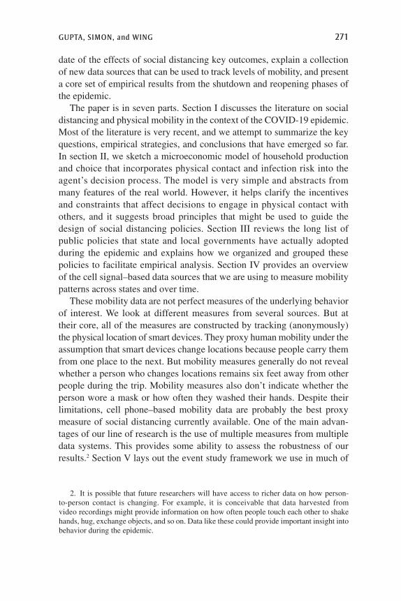
The state policies adopted during the shutdown phase occurred very rapidly. With an eye toward econometric models, we worked to understand the order and timing of the sequence of policies and to assess the extent to which it is feasible to meaningfully separate the effects of different poli-cies. Figure 1 shows how the share of the US population that was subject to each social distancing policy evolved over time.10
Emergency declarations appear early and separate from the other poli-cies. However, school closures, gathering restrictions, and restaurant and nonessential business closings often coincide so closely in time that it seems infeasible to identify their effects separately in a regression analysis. Given the information on the sequence and timing of state policies, we condensed the six major policy events to a set of four major events during the shutdown phase: state first cases and deaths, emergency declarations, school closures, and stay-at-home mandates.
As this section demonstrates, there are some principles we use for select-ing which of the large number of different state policies currently discussed in the COVID-19 policy literature we should track in our research on mobility. The key decision factor was ensuring close connections to our theoretic framework while considering (informally) whether we could plausibly separate the effects of these policies.
III.B. Typology of Reopening Policies
We collected and coded data on state reopening policies, starting with descriptions of reopening plans in the New York Times. We gathered addi-tional information on the reopening schedules for each state through internet searches.11 We consider two primary reopening dates: date of announcement of upcoming reopenings and date of actual reopening. We define the state’s reopening date as the earliest date at which that state issued a reopening policy of any type. The dates we determined as the first reopening event for
10. Figure 2.2 in Gupta, Nguyen, and others (2020) shows the timeline of the policy changes that occurred in each state, and figure 3.2 shows the timing of the first cases and deaths by state. There we show that the first COVID-19 case in a state is easily set apart in timing from the other policies, as is the first COVID-19 death.
11. We provide the reopening policies information we have compiled from various sources at https://github.com/nguyendieuthuy/ReOpeningPlans.

GUPTA, SIMON, and WING 289
US population (percent)
Source: Authors’ compilations.Note: Data cover January 20 to June 15, 2020.
US population (percent)
Time4/25/20 5/5/20 5/15/20 5/25/20 6/4/20 6/14/20
80
100
60
40
20
Any business reopening
Reopening in retail
Nonessentialbusinessclosure
Stay-at-home
School closures
Gatheringrestrictions
Emergency declarations
First case recorded
Restaurant/business
Reopening three or more sectors
Reopening two or fewer sectors
Time1/27/20 2/10/20 2/24/20 3/9/20 3/23/20 4/6/20
80
100
60
40
20
Figure 1. US Population Covered by State Closure and Reopening Policies
290 Brookings Papers on Economic Activity, Summer 2020
each state are identical to the ones depicted in figures used by the New York Times.12 Starting with South Carolina, by June 15, all states had officially reopened in some phased form.
Some states never formally adopted a stay-at-home order, but even these states implemented partial business closures (e.g., restaurant closures) and some nonessential business restrictions. Of course, measures of mobility and economic activity have fallen in these states as well because of private social distancing choices. In addition, the lack of an official closure does not mean that state governments cannot take actions to try to hasten the return to regular levels of activity. For example, South Dakota did not have a statewide stay-at-home order, but the governor announced a “back to normal” plan that set May 1 as the reopening date for many businesses. Our study period to examine the effect of reopenings on mobility commences on April 15 to ensure that we capture reopenings across all states.
Most reopening policies have been centered around seven areas of economic activity: outdoor recreation, retail, restaurant, worship, personal care, entertainment, and industry activities. However, the pace at which states have reopened each of these sectors has varied a lot. Some states reopened most businesses and industries immediately, while others have adopted a much more phased approach.13 Retail, recreation, and restaurants have often reopened first, frequently only at limited capacity (see figure 1).
South Carolina was the first state to reopen, on April 20. It was also one of the last states to adopt a stay-at-home order.14 This April 20 reopening was partial, allowing retail stores to open at 20 percent of capacity. By April 30, twelve states had reopened to some degree (Alabama, Mississippi, Tennessee, Montana, Oklahoma, Alaska, Georgia, Michigan, Minnesota, Vermont, Wisconsin, and South Carolina). Eleven more states reopened on May 1; by May 13, a total of forty states had reopened. By June 30 all states had undergone at least the first stage of reopening. In most of our reopening analyses the study period ends on June 15, which means that we are able to estimate impacts for at least thirty days post-reopening using variation from all fifty states and the District of Columbia for phase 1 and phase 2 reopening policies.
12. “See Coronavirus Restrictions and Mask Mandates for All 50 States,” New York Times, https://www.nytimes.com/interactive/2020/us/states-reopen-map-coronavirus.html, accessed June 23, 2020.
13. Alaska, Connecticut, Washington, D.C., Iowa, Indiana, Louisiana, Maryland, Missouri, New Hampshire, Nevada, South Dakota, and Wyoming reopened initially by opening five or more of the seven sectors.
14. Although it issued an emergency declaration fairly early (March 13), South Carolina did not issue a stay-at-home order until April 7 (see Gupta, Nguyen, and others 2020).

GUPTA, SIMON, and WING 291
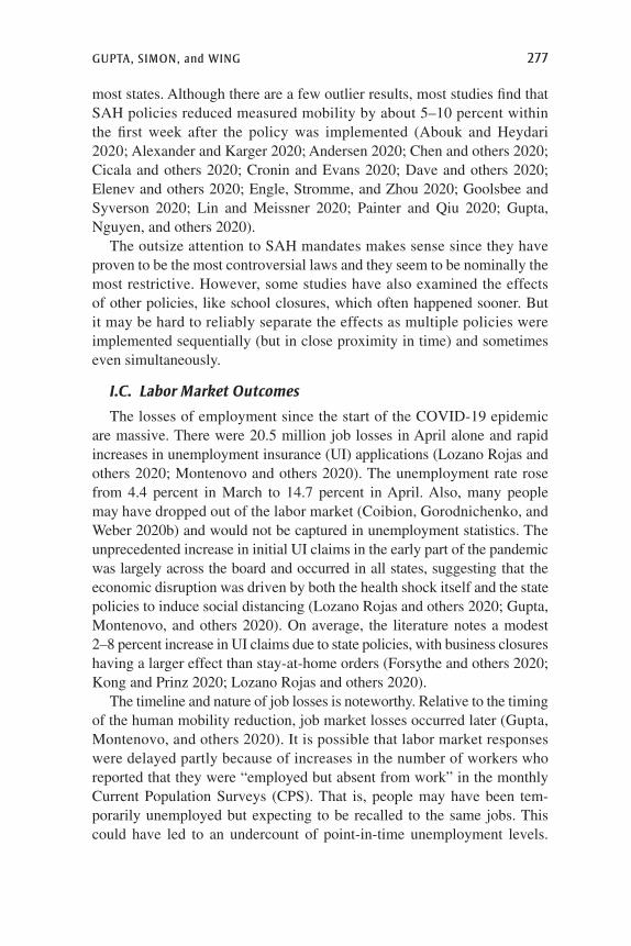
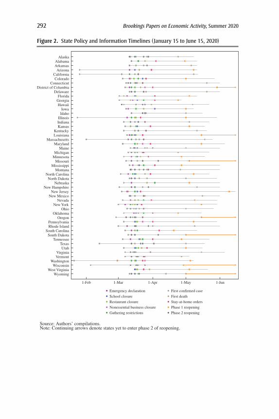
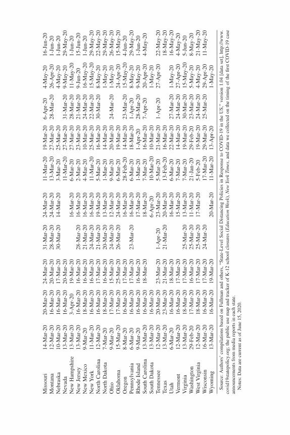
Stay-at-home orders and nonessential business closures are related but distinct. Several states issued stay-at-home mandates after they issued orders closing all nonessential businesses or after closing some nonessen-tial businesses (such as gyms) and closing restaurants for on-site dining. Although for the most part, stay-at-home orders coincided with orders to close all nonessential businesses, restaurants and other select categories of business closures started well before stay-at-home orders. Many business closures started in mid-March, along with school closures (see figure 2). Timing of reopenings has been within 24 hours of lifting stay-at-home orders in only seven states (Connecticut, Florida, Idaho, Kansas, Montana, Pennsylvania, and Utah; see table 1 for details).15 In the remaining states, reopening frequently preceded official expiry of stay-at-home orders on average by a month (thirty-two days).
The top panel of figure 1 shows that by June 15 all US states had adopted some form of reopening policy. However, the pace of reopening has been gradual and varied. The bottom panel of figure 1 shows that by June 15, nearly 74 percent of the population lives in states that opened the retail sector, but only 60 percent is in states that opened three or more sectors that we track.16 However, seventeen states pursued a more limited strategy by opening only one or two sectors.17
States that either implemented fewer social distancing measures or implemented those measures later also tended to reopen earlier, based on time since the first of four major social distancing measures—nonessential business closures, restaurant closures, social gathering restrictions, and stay-at-home orders or advisories. These results may reflect either a lack of political desire to engage in distancing or a more limited outbreak (Andersen 2020; Adolph and others 2020; Allcott and others 2020).
IV. Mobility Data
The data sets typically used in public health research do not provide high-frequency measures of social interaction. To make progress, our research program has made heavy use of data from at least four commercial cell signal aggregators who have provided their data for free to support COVID-19
15. COVID-19 US State Policy Database, www.tinyurl.com/statepolicies.16. Following the New York Times, we track outdoor recreation, retail, food and drink
establishments, personal care establishments, houses of worship, entertainment venues, and industrial areas.
17. There were seven states where we could not clearly identify the sectors that would be affected by the reopening decision.
292 Brookings Papers on Economic Activity, Summer 2020
Source: Authors’ compilations.Note: Continuing arrows denote states yet to enter phase 2 of reopening.
AlaskaAlabamaArkansasArizona
CaliforniaColorado
ConnecticutDistrict of Columbia
DelawareFlorida
GeorgiaHawaii
IowaIdaho
IllinoisIndianaKansas
KentuckyLouisiana
MassachusettsMaryland
MaineMichigan
MinnesotaMissouri
MississippiMontana
North CarolinaNorth Dakota
NebraskaNew Hampshire
New JerseyNew Mexico
NevadaNew York
OhioOklahoma
OregonPennsylvaniaRhode Island
South CarolinaSouth Dakota
TennesseeTexasUtah
VirginiaVermont
WashingtonWisconsin
West VirginiaWyoming
1-Feb 1-Mar 1-Apr 1-May 1-Jun
Emergency declaration
School closure
Restaurant closure
Nonessential business closure
Gathering restrictions
First confirmed case
First death
Stay-at-home orders
Phase 1 reopening
Phase 2 reopening
Figure 2. State Policy and Information Timelines (January 15 to June 15, 2020)
GUPTA, SIMON, and WING 293
research. Each company has several different measures of mobility, which may capture a different form of underlying behavior, with different impli-cations for the transmission of the virus and economic activity. In addition, each company collects data from potentially different sets of app users, and it is possible that some of the cell signal panels are more mobile than others. Given these complexities, it is important to examine several measures of mobility both to assess the robustness and generality of a result and to provide opportunities to learn from differences in results across measures. In this paper, we discuss results based on data from Apple’s Mobility Trends Reports, Google’s Community Mobility Reports, PlaceIQ, and SafeGraph.
Apple’s Mobility Trends Reports are published daily and reflect requests for driving directions in Apple Maps.18 The measure we use tracks the volume of driving directions requests per US state compared to a baseline volume on January 13, 2020; no county-level equivalent is available.
We extract state-level measures of mobility from Google’s Community Mobility Reports, which contain county-level data as well.19 We use the data that reflect the percent change in visits to places within a geographic area, including grocery and pharmacy, transit stations (public transport hubs such as subway, bus, and train stations), retail and recreation (e.g., restaurants, shopping centers, and theme parks), places of work, and resi-dential (places of residence). The baseline for computing these changes is the median level of activity on the corresponding day of the week from January 3 to February 6, 2020.
We use two anonymized, aggregated location exposure indexes from PlaceIQ data: (1) a mixing index that, for a given day, detects the likely exposure of a smart device to other devices in a county or state on a given day, and (2) out-of-state and out-of-county travel indexes that measure, among smart devices that pinged in a given geographic location, the percent of these devices that pinged in another geographic location at least once during the previous fourteen days.20
18. Apple Mobility Trends Reports, https://www.apple.com/covid19/mobility, accessed June 22, 2020.
19. Google, COVID-19 Community Mobility Reports, 2020, https://www.google.com/covid19/ mobility, accessed June 22, 2020.
20. Victor Couture, Jonathan I. Dingel, Allison E. Green, Jessie Handbury, and Kevin R. Williams, Exposure Indices Derived from PlaceIQ Movement Data [data set], 2020, https://github.com/COVIDExposureIndices/COVIDExposureIndices.

Tabl
e 1.
Sta
te S
ocia
l Dis
tanc
ing–
Rel
ated
Pol
icy
Enac
tmen
t and
Info
rmat
ion
Even
t Dat
es
Em
erge
ncy
decl
arat
ions
Scho
olcl
osur
es
Res
taur
ant/
othe
rre
stri
ctio
ns
Gat
heri
ngre
stri
ctio
ns
(any
)
Non
esse
ntia
lbu
sine
ss
clos
ures
Fir
st
confi
rmed
case
Fir
stde
ath
Stay
-at-
hom
e or
ders
Init
ial
reop
enin
gsP
hase
2re
open
ings
Ala
bam
a11
-Mar
-20
16-M
ar-2
017
-Mar
-20
28-M
ar-2
024
-Mar
-20
12-M
ar-2
027
-Mar
-20
4-A
pr-2
030
-Apr
-20
11-M
ay-2
0A
lask
a13
-Mar
-20
19-M
ar-2
020
-Mar
-20
20-M
ar-2
013
-Mar
-20
25-M
ar-2
028
-Mar
-20
24-A
pr-2
08-
May
-20
Ari
zona
11-M
ar-2
017
-Mar
-20
19-M
ar-2
011
-Mar
-20
24-M
ar-2
031
-Mar
-20
8-M
ay-2
011
-May
-20
Ark
ansa
s11
-Mar
-20
16-M
ar-2
020
-Mar
-20
26-J
an-2
020
-Mar
-20
6-M
ay-2
011
-May
-20
Cal
ifor
nia
4-M
ar-2
019
-Mar
-20
15-M
ar-2
019
-Mar
-20
11-M
ar-2
026
-Jan
-20
4-M
ar-2
019
-Mar
-20
8-M
ay-2
012
-May
-20
Col
orad
o10
-Mar
-20
23-M
ar-2
017
-Mar
-20
26-M
ar-2
019
-Mar
-20
5-M
ar-2
012
-Mar
-20
26-M
ar-2
01-
May
-20
27-M
ay-2
0C
onne
ctic
ut10
-Mar
-20
17-M
ar-2
016
-Mar
-20
23-M
ar-2
012
-Mar
-20
8-M
ar-2
018
-Mar
-20
23-M
ar-2
020
-May
-20
17-J
un-2
0D
elaw
are
11-M
ar-2
016
-Mar
-20
16-M
ar-2
025
-Mar
-20
13-M
ar-2
07-
Mar
-20
21-M
ar-2
024
-Mar
-20
20-M
ay-2
015
-Jun
-20
DC
13-M
ar-2
016
-Mar
-20
16-M
ar-2
024
-Mar
-20
16-M
ar-2
011
-Mar
-20
26-M
ar-2
01-
Apr
-20
29-M
ay-2
0F
lori
da9-
Mar
-20
16-M
ar-2
017
-Mar
-20
30-M
ar-2
03-
Apr
-20
2-M
ar-2
06-
Mar
-20
3-A
pr-2
04-
May
-20
5-Ju
n-20
Geo
rgia
14-M
ar-2
018
-Mar
-20
24-M
ar-2
024
-Mar
-20
2-M
ar-2
012
-Mar
-20
3-A
pr-2
024
-Apr
-20
27-A
pr-2
0H
awai
i4-
Mar
-20
23-M
ar-2
017
-Mar
-20
25-M
ar-2
016
-Mar
-20
6-M
ar-2
031
-Mar
-20
25-M
ar-2
07-
May
-20
22-M
ay-2
0Id
aho
9-M
ar-2
03-
Apr
-20
17-M
ar-2
017
-Mar
-20
8-M
ar-2
024
-Mar
-20
25-M
ar-2
01-
May
-20
16-M
ay-2
0Il
lino
is13
-Mar
-20
23-M
ar-2
025
-Mar
-20
25-M
ar-2
025
-Mar
-20
13-M
ar-2
026
-Mar
-20
21-M
ar-2
01-
May
-20
29-M
ay-2
0In
dian
a9-
Mar
-20
17-M
ar-2
016
-Mar
-20
21-M
ar-2
013
-Mar
-20
24-J
an-2
017
-Mar
-20
25-M
ar-2
04-
May
-20
22-M
ay-2
0Io
wa
6-M
ar-2
019
-Mar
-20
16-M
ar-2
024
-Mar
-20
12-M
ar-2
06-
Mar
-20
16-M
ar-2
01-
May
-20
8-M
ay-2
0K
ansa
s12
-Mar
-20
18-M
ar-2
017
-Mar
-20
7-M
ar-2
012
-Mar
-20
30-M
ar-2
04-
May
-20
18-M
ay-2
0K
entu
cky
6-M
ar-2
016
-Mar
-20
16-M
ar-2
026
-Mar
-20
19-M
ar-2
06-
Mar
-20
16-M
ar-2
026
-Mar
-20
11-M
ay-2
020
-May
-20
Lou
isia
na11
-Mar
-20
16-M
ar-2
017
-Mar
-20
23-M
ar-2
013
-Mar
-20
9-M
ar-2
014
-Mar
-20
23-M
ar-2
015
-May
-20
5-Ju
n-20
Mai
ne10
-Mar
-20
17-M
ar-2
017
-Mar
-20
24-M
ar-2
013
-Mar
-20
1-F
eb-2
020
-Mar
-20
1-A
pr-2
01-
May
-20
1-Ju
n-20
Mar
ylan
d5-
Mar
-20
16-M
ar-2
016
-Mar
-20
23-M
ar-2
016
-Mar
-20
5-M
ar-2
018
-Mar
-20
30-M
ar-2
015
-May
-20
5-Ju
n-20
Mas
sach
uset
ts15
-Mar
-20
16-M
ar-2
018
-Mar
-20
25-M
ar-2
018
-Mar
-20
12-M
ar-2
027
-Mar
-20
24-M
ar-2
018
-May
-20
8-Ju
n-20
Mic
higa
n10
-Mar
-20
16-M
ar-2
016
-Mar
-20
23-M
ar-2
013
-Mar
-20
10-M
ar-2
018
-Mar
-20
24-M
ar-2
024
-Apr
-20
22-M
ay-2
0M
inne
sota
13-M
ar-2
018
-Mar
-20
17-M
ar-2
06-
Mar
-20
21-M
ar-2
028
-Mar
-20
27-A
pr-2
018
-May
-20
Mis
siss
ippi
13-M
ar-2
023
-Mar
-20
17-M
ar-2
023
-Mar
-20
8-M
ar-2
018
-Mar
-20
3-A
pr-2
027
-Apr
-20
1-Ju
n-20
Mis
sour
i14
-Mar
-20
20-M
ar-2
024
-Mar
-20
31-M
ar-2
024
-Mar
-20
11-M
ar-2
019
-Mar
-20
6-A
pr-2
04-
May
-20
16-J
un-2
0M
onta
na12
-Mar
-20
16-M
ar-2
020
-Mar
-20
28-M
ar-2
024
-Mar
-20
13-M
ar-2
027
-Mar
-20
28-M
ar-2
026
-Apr
-20
1-Ju
n-20
Neb
rask
a10
-Mar
-20
16-M
ar-2
017
-Mar
-20
30-M
ar-2
014
-Mar
-20
3-M
ar-2
025
-Mar
-20
4-M
ay-2
01-
Jun-
20N
evad
a13
-Mar
-20
16-M
ar-2
020
-Mar
-20
11-M
ar-2
027
-Mar
-20
31-M
ar-2
09-
May
-20
29-M
ay-2
0N
ew H
amps
hire
13-M
ar-2
03-
Apr
-20
19-M
ar-2
016
-Mar
-20
6-M
ar-2
027
-Mar
-20
28-M
ar-2
011
-May
-20
1-Ju
n-20
New
Jer
sey
13-M
ar-2
016
-Mar
-20
16-M
ar-2
028
-Mar
-20
16-M
ar-2
02-
Mar
-20
23-M
ar-2
021
-Mar
-20
9-Ju
n-20
15-J
un-2
0N
ew M
exic
o9-
Mar
-20
18-M
ar-2
016
-Mar
-20
21-M
ar-2
016
-Mar
-20
4-M
ar-2
010
-Mar
-20
24-M
ar-2
016
-May
-20
1-Ju
n-20
New
Yor
k11
-Mar
-20
16-M
ar-2
016
-Mar
-20
24-M
ar-2
016
-Mar
-20
11-M
ar-2
025
-Mar
-20
22-M
ar-2
015
-May
-20
29-M
ay-2
0N
orth
Car
olin
a12
-Mar
-20
16-M
ar-2
017
-Mar
-20
21-M
ar-2
019
-Mar
-20
5-M
ar-2
016
-Mar
-20
30-M
ar-2
08-
May
-20
22-M
ay-2
0N
orth
Dak
ota
7-M
ar-2
018
-Mar
-20
16-M
ar-2
020
-Mar
-20
13-M
ar-2
01-
Mar
-20
14-M
ar-2
01-
May
-20
29-M
ay-2
0O
hio
9-M
ar-2
017
-Mar
-20
15-M
ar-2
024
-Mar
-20
12-M
ar-2
09-
Mar
-20
20-M
ar-2
024
-Mar
-20
1-M
ay-2
026
-May
-20
Okl
ahom
a15
-Mar
-20
17-M
ar-2
025
-Mar
-20
26-M
ar-2
024
-Mar
-20
6-M
ar-2
019
-Mar
-20
24-A
pr-2
015
-May
-20
Ore
gon
8-M
ar-2
016
-Mar
-20
17-M
ar-2
016
-Mar
-20
28-F
eb-2
014
-Mar
-20
23-M
ar-2
015
-May
-20
4-Ju
n-20
Pen
nsyl
vani
a6-
Mar
-20
16-M
ar-2
017
-Mar
-20
23-M
ar-2
016
-Mar
-20
6-M
ar-2
018
-Mar
-20
1-A
pr-2
08-
May
-20
29-M
ay-2
0R
hode
Isl
and
9-M
ar-2
016
-Mar
-20
16-M
ar-2
017
-Mar
-20
1-M
ar-2
01-
Apr
-20
28-M
ar-2
09-
May
-20
1-Ju
n-20
Sou
th C
arol
ina
13-M
ar-2
016
-Mar
-20
18-M
ar-2
018
-Mar
-20
7-M
ar-2
016
-Mar
-20
7-A
pr-2
020
-Apr
-20
4-M
ay-2
0S
outh
Dak
ota
13-M
ar-2
016
-Mar
-20
6-A
pr-2
010
-Mar
-20
10-M
ar-2
01-
May
-20
Tenn
esse
e12
-Mar
-20
20-M
ar-2
023
-Mar
-20
1-A
pr-2
023
-Mar
-20
5-M
ar-2
021
-Mar
-20
1-A
pr-2
027
-Apr
-20
22-M
ay-2
0Te
xas
13-M
ar-2
023
-Mar
-20
21-M
ar-2
021
-Mar
-20
20-M
ar-2
013
-Feb
-20
16-M
ar-2
018
-May
-20
Uta
h6-
Mar
-20
16-M
ar-2
018
-Mar
-20
16-M
ar-2
06-
Mar
-20
22-M
ar-2
027
-Mar
-20
1-M
ay-2
016
-May
-20
Ver
mon
t12
-Mar
-20
16-M
ar-2
017
-Mar
-20
15-M
ar-2
07-
Mar
-20
14-M
ar-2
024
-Mar
-20
27-A
pr-2
04-
May
-20
Vir
gini
a13
-Mar
-20
18-M
ar-2
017
-Mar
-20
25-M
ar-2
013
-Mar
-20
7-M
ar-2
019
-Mar
-20
30-M
ar-2
015
-May
-20
5-Ju
n-20
Was
hing
ton
29-F
eb-2
017
-Mar
-20
16-M
ar-2
025
-Mar
-20
11-M
ar-2
021
-Jan
-20
29-F
eb-2
023
-Mar
-20
5-M
ay-2
08-
May
-20
Wes
t Vir
gini
a12
-Mar
-20
18-M
ar-2
017
-Mar
-20
25-M
ar-2
017
-Mar
-20
5-F
eb-2
019
-Mar
-20
24-M
ar-2
04-
May
-20
21-M
ay-2
0W
isco
nsin
16-M
ar-2
016
-Mar
-20
17-M
ar-2
024
-Mar
-20
17-M
ar-2
029
-Mar
-20
25-M
ar-2
029
-Apr
-20
11-M
ay-2
0W
yom
ing
13-M
ar-2
016
-Mar
-20
19-M
ar-2
020
-Mar
-20
11-M
ar-2
013
-Apr
-20
1-M
ay-2
0
Sour
ce: A
utho
rs’
com
pila
tions
bas
ed o
n Fu
llman
and
oth
ers,
“St
ate-
Lev
el S
ocia
l D
ista
ncin
g Po
licie
s in
Res
pons
e to
CO
VID
-19
in t
he U
S,”
vers
ion
1.04
[da
ta s
et],
http
://w
ww
.co
vid1
9sta
tepo
licy.
org;
the
publ
ic u
se m
ap a
nd tr
acke
r of
K-1
2 sc
hool
clo
sure
s (E
duca
tion
Wee
k), N
ew Y
ork
Tim
es, a
nd d
ata
we
colle
cted
on
the
timin
g of
the
first
CO
VID
-19
case
an
noun
cem
ents
fro
m m
edia
rep
orts
in e
ach
stat
e.N
otes
: Dat
a ar
e cu
rren
t as
of J
une
15, 2
020.

296 Brookings Papers on Economic Activity, Summer 2020
We use SafeGraph data to measure the median hours spent at home by devices as well as the number of devices at the census block group level that are detected at a typical work location during the day or to have left the house. We aggregate these to state by-day levels.
V. Econometric Framework
Let Yst be a measure of mobility in state s on date t. Es is the start date of a closure/reopening policy in state s. TSEst = t − Es is the number of days between t and the adoption date. We fit the following event study regres-sion model:
Y TSE a TSE b Wst a sta b st st s t stb∑ ∑( ) ( )= α = − + β = + σ + q + γ += −
−
=1 1 .
30
2
0
30
In the model, qs is a state fixed effect, which captures time-invariant dif-ferences in outcomes across states. γt is a date fixed effect, which represents a common trend. Wst is a vector of state times day measures of temperature and precipitation, which helps adjust for seasonality. st is a residual error term, and αa and βb trace out deviations from the common trends that states experience in the days leading up to and following a given policy event. Standard errors allow for clustering at the state level.
Our main specifications are based on a balanced panel of states. The models are not weighted, and our estimates reflect the average state rather than the average person. The composition of states contributing to event study coefficients is quite stable for a range of thirty days before and after the event. The calendar time covered by the event studies varies some-what across outcomes and is described along with each set of results. To help summarize results, we assess the presence of a pre-trend based on the statistical significance of the pre-policy event study coefficients. In our summary results, we say that a measure exhibits a pre-trend if at least 30 percent of the coefficients in the pre-period were statistically significant.
We also use the event study models to decompose the overall change in mobility over time into a share explained by state-level policy changes and a share explained by secular trends that are not associated with state policies. To understand the counterfactual exercise, let yst be the fitted value for state s on date t from the estimated event study regression. These fitted values are a model-based estimate of what actually happened in the state. Let yst* = �yst − ∑30
b=0 βb1(TSEst = b) be an estimate of the counterfactual mobility

GUPTA, SIMON, and WING 297
outcome that would have prevailed in the absence of the state policy. We compute the daily cross-state average of the fitted values and counter-factual estimates to form two national time series of mobility outcomes. A close correspondence between the realized time series and the counter-factual time series would indicate that changes in mobility are mainly from secular trends rather than policy.
VI. Results
VI.A. Trends in Mobility
The collection of graphs in figure 3 shows the national and state-level time series for a subset of the mobility measures we follow in Gupta, Nguyen, and others (2020) and Nguyen and others (2020). The dashed black line indicates the “smoothed” (seven-day moving average) national average (not weighted by state population). Each of the lines on a graph represents a state. The state lines darken in the middle for the time period when the state implemented a stay-at-home (SAH) order, and then they change again when the state implements its first reopening stage. This provides a conve-nient way to observe when the changes in mobility occurred relative to the policy dates.
The overall pattern of results is very consistent across the different measures of mobility. The top left panel of figure 3 shows the mixing index. Weekend patterns and other seasonal effects are visible, when all lines move together. There is a substantial drop in mixing around mid-March, when the index falls more than 73.4 percent between March 1 and April 14. The top right panel of figure 3 shows the average out-of-county travel measure, which fell by 33.4 percent between March 1 and April 14. The bottom left panel of figure 3 shows trends for hours spent at home, which is a state-level average of census block group medians. Time at home increased 60.6 percent between March 1 and April 14. The springtime is typically associated with more mobility and interaction, so any decline during this period is abnormal.21
The graphs in figure 3 show that states with no SAH mandates also experienced large declines in mobility as well as subsequent increases after
21. Data for recent years (2018–2019) from the US Department of Transportation for (seasonally unadjusted) vehicle miles traveled show that the March value is typically 20 per-cent higher than February’s value (US Department of Transportation 2020).

298 Brookings Papers on Economic Activity, Summer 2020
Source: Authors’ calculations based on data from Apple Mobility, Google Mobility, SafeGraph Aggregated Mobility Metrics, and PlaceIQ smart device.
Notes: Each line represents a state, indicating when the state implemented stay-at-home orders (middle) and change after phase 1 of reopening (right). The thick black line represents a smoothed seven-day moving average of the states.
Median hours at home
(g) Median hours at home (h) Fraction leaving homeFraction left the house
Source: SafeGraph Aggregated Mobility Metrics Source: SafeGraph Aggregated Mobility Metrics
06mar2020 15apr2020 25may2020
10
15
06mar2020 15apr2020 25may20200.5
0.6
0.7
0.8
Mobility to retail/recreation
(e) Retail and recreation (f) Grocery and pharmacyMobility to grocery/pharmacy
Source: Google Mobility Source: Google Mobility
06mar2020 15apr2020 25may2020
–40
–20
0
–6006mar2020 15apr2020 25may2020
0
20
–20
Request for driving direction
(c) Requests for driving directions (d) Fraction at workFraction at work
Source: Apple Mobility Source: SafeGraph Aggregated Mobility Metrics
100
150
200
5006mar2020 15apr2020 25may2020
0.15
0.20
0.10
16mar2020 15apr2020 15may2020
Mixing index
(a) Mixing index (b) Average out-of-county movementTotal out-of-county movement
Source: PlaceIQ Source: PlaceIQY-axis is truncated at 400
06mar2020 15apr2020 25may2020
100
200
300
06mar2020 15apr2020 25may2020
2
4
3
Figure 3. Trend in Mobility Changes
GUPTA, SIMON, and WING 299
mid-April. Indeed, states with no SAH policies at all had declines in move-ment almost as dramatic as in other states. Furthermore, most states with SAH mandates experienced major declines in mobility even before the SAH mandates went into effect.
VI.B. Mandate Effects
Estimates of the event studies evaluating the effect of closure policies and informational events on each of the mobility measures are presented in Gupta, Nguyen, and others (2020). In figure 4 we graphically present the event study coefficients of the effect of state policies and informational events on the mixing index available from PlaceIQ. As noted in section IV the mixing index captures the concentration of devices in particular loca-tions and provides the closest proxy for social distancing and thus trans-mission. The results suggest that the concentration of devices in particular locations does not trend differentially in the period leading up to any policy or information event. However, we do not find statistically significant evidence that the policy or information events have induced substantial changes in mixing at the state level except for a large effect of emergency declarations. The event study coefficients imply that emergency declara-tions reduced the state-level mixing index by about 52 percent after twenty days, relative to the value of the index on March 1, which is the baseline reference period for all percent effects reported for closure events. The coefficients show a similar pattern for first deaths, but it is not statistically significant.
Table 2 provides a summary of the results of the event study regressions for each outcome and policy or information event, including additional ones for which figures and tables of coefficients are reported in Gupta, Nguyen, and others (2020). Table 2 has a row for each state outcome variable and a column for each policy or information event. The top panel shows the effect size five days after the event, expressed as a per-centage of the average value of the outcome variable on March 1, 2020. The bottom panel shows the effect size after twenty days, also expressed as a percentage of the average outcome on March 1. We indicate the effects that are statistically significant at the 5 percent level or better and where parallel trends hold. The cells that are shaded in grey have possible viola-tions of the differential pre-trends assumption and should be largely over-looked; we do not indicate statistical significance for them. First death announcements also carry a large coefficient but it is statistically not signifi-cant; school closures and stay-at-home laws have statistically insignificant and wrong-signed coefficients.
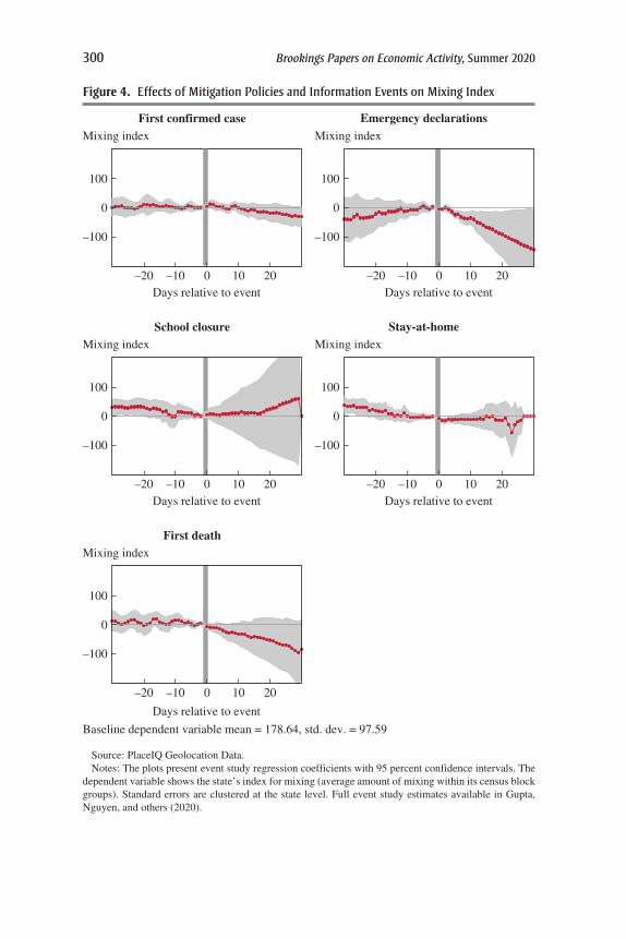
300 Brookings Papers on Economic Activity, Summer 2020
Source: PlaceIQ Geolocation Data.Notes: The plots present event study regression coefficients with 95 percent confidence intervals. The
dependent variable shows the state’s index for mixing (average amount of mixing within its census block groups). Standard errors are clustered at the state level. Full event study estimates available in Gupta, Nguyen, and others (2020).
First deathMixing index
–20 –10 0 10 20
0
100
–100
Days relative to event
School closure Stay-at-homeMixing index
–20 –10 0 10 20
0
100
–100
Days relative to event
Mixing index
–20 –10 0 10 20
0
100
–100
Days relative to event
First confirmed case Emergency declarationsMixing index
–20 –10 0 10 20
0
100
–100
Days relative to event
Mixing index
–20 –10 0 10 20
0
100
–100
Days relative to event
Baseline dependent variable mean = 178.64, std. dev. = 97.59
Figure 4. Effects of Mitigation Policies and Information Events on Mixing Index

GUPTA, SIMON, and WING 301
Table 2. Effect Sizes: Percentage Magnitude Effects of the Policy and Informational Events on Social Distancing Measures
1. Effects of mitigation policies and informational events
First confirmed
caseEmergency
declarationsSchool
closuresStay-at-
homeFirst death
Effects after 5 days
Mixing index 1 −14*** 4 −7 −11Median hours at home −1* 6*** 1 5 3*Fraction leaving home 1** −1* −1 −5 −2***Total out-of-state movement −2 −1 −4** −1 0Total out-of-county movement −1 −2** −4*** −3 −2
Effects after 20 days
Mixing index −10 −52*** 13 −8 −31Median hours at home −2 27*** 3 11 9**Fraction leaving home 2 −13*** −3 −9 −7***Total out-of-state movement −9 −3 −13 1 5Total out-of-county movement −2 −8*** −9*** −2 −6*
2. Effects of state initial reopenings
Announcement ofinitial reopening
Initial reopening
Effects after 5 days
Mobility measures (%) (%)Request for driving directions −6 −3Mobility to retail/recreation 3 3Mobility to grocery/pharmacy 8 9Mobility to transit stations 0 9Mobility to workplace 2 3**Fraction at work −3* 2Fraction left home 1** 1**Mixing index −2 5Out-of-state movement −2 0Out-of-county movement −1 0
Absence of mobility measuresStay in residential areas −1 −4**Median hours at home −1* −1***
(continued on next page)

302 Brookings Papers on Economic Activity, Summer 2020
VI.C. Reopening Effects
In a manner similar to the event studies for the closure policies, we present results for the initial reopening dates, starting in figure 5. The two panels display effects first where the policy date is the announcement of the reopening and second for the actual reopening date. There is a pattern (although not statistically significant) of what appears to be a nonparallel trend prior to the actual reopening date, but it is fairly flat prior to the announcement date. None of the estimates are statistically significant, even after the policy is effective, although nonsignificant coefficients are consis-tent with an increase in movement after the announcement date. This helps illustrate our finding that it is important to consider a variety of mobility measures to assess the impact of the policies. Table 2 shows that although the mixing index is not statistically precise, there are several other outcomes that are and that do not violate pre-trends concerns. The effect sizes here are, however, considerably smaller than in the closure period. One reason for that may be that in the reopening phase we do not have informational
Table 2. Effect Sizes: Percentage Magnitude Effects of the Policy and Informational Events on Social Distancing Measures
Announcement ofinitial reopening
Initial reopening
Effects after 20 days
Mobility measures (%) (%)Request for driving directions −15 −15Mobility to retail/recreation 8 4Mobility to grocery/pharmacy 8 4Mobility to transit stations 0 −6Mobility to workplace 4 1Fraction at work 2 1Fraction left home 4*** 1Mixing index 20 −4Out-of-state movement −1 −8Out-of-county movement 2 0
Absence of mobility measures (%) (%)Stay in residential areas −5 −4Median hours at home −3*** −3***
Source: Authors’ calculations.Notes: Each cell is from a separate regression. Grey-shaded cells denote violation of pretreatment
parallel trends—we do not denote statistical significance for these cells. Effect sizes for closures are esti-mated using coefficients in the event study tables presented in Gupta, Nguyen, and others (2020), divided by the dependent variable value as of March 1, 2020. Effect sizes for reopenings are estimated using coefficients in the event study tables presented in Nguyen and others (2020), divided by the dependent variable value as of April 15, 2020.
*** p < .01; ** p < .05; * p < .10.
(Continued)

GUPTA, SIMON, and WING 303
Initial reopeningMixing index
Source: PlaceIQ (April 9 to June 11, 2020).Notes: The plots present event study regression coefficients with 95 percent confidence intervals. The
dependent variable shows the state’s index for mixing (average amount of mixing within its census block groups). Standard errors are clustered at the state level. Full event study estimates available in Nguyen and others (2020).
Baseline DV mean = 44.02, std. dev. = 19.31Days relative to reopening
–26 –22 –18 –14 –10 –6 –2 2 6 10 14 18 22 26
0
20
40
Announcement of initial reopeningMixing index
Baseline DV mean = 44.02, std. dev. = 19.31Days relative to reopening
–26 –22 –18 –14 –10 –6 –2 2 6 10 14 18 22 26
0
20
40
Figure 5. Effects of Announcement and Effective Date of Initial Reopening on Mixing Index

304 Brookings Papers on Economic Activity, Summer 2020
events occurring in the same way they did during the closure period. We do not study the impact of changing rates of COVID-19 cases or deaths, as those were often directly referred to as conditions for reopening.
The overall message from table 2 for the reopening dates is that esti-mates are fairly similar whether we use the announcement date or the actual reopening date and that effect sizes are fairly small at both five days and twenty days, on the order of 1–4 percent. These are not surprising results, given the very limited nature of initial reopening phases. The small effects overall also could mask larger effects in certain situations; event study estimates are summaries of each state’s experience (Wing, Simon, and Bello-Gomez 2018), and Nguyen and others (2020) show that effects are larger in states that were the last to close businesses and also differ along a number of other dimensions.
VI.D. The Role of Secular Trends (National Sentiment)
One way to interpret our results is to use the event study coefficients to tease apart the amount of the actual change in mobility that occurred during the closure or reopening time periods into shares explained by state actions, relative to secular changes in sentiment due to other factors. Figure 6 and table 3 show estimates of this decomposition for the mixing index during the shutdown phase. We used event study regressions to esti-mate the effects of emergency declarations on the mixing index outcome. The solid line in figure 6 shows how the national average mixing index actually changed over time. The dashed line is an estimate of the counter-factual path of the mixing index, which removes the policy effects from the model. The time trends captured by the model imply that the mixing index would have increased substantially in the absence of the emergency declarations. Table 3 shows that the emergency declaration event study coefficients account for about 65 percent of the observed decline in the mixing index that occurred between the first week of March and the second week of April. The remaining 35 percent was due to secular trends that occurred separately from state emergency declarations. Decompositions like this one imply that both policy and private responses (secular trends) played a key role during the shutdown. However, the specific policy share versus secular share varies across measures of mobility.
We used this same strategy to examine the state reopening policies. Figure 7 and table 4 show decomposition results for the mixing index and the fraction of people who leave home during the day. The solid lines in figure 7 show how the mixing index (top panel) and the fraction leaving home (bottom panel) evolved between mid-April and mid-June. Both
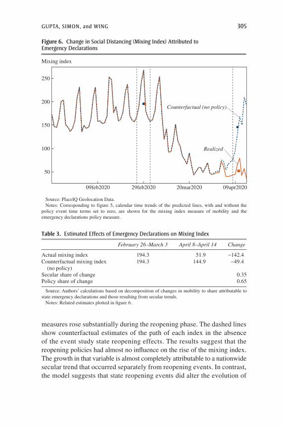
GUPTA, SIMON, and WING 305
Mixing index
Realized
Counterfactual (no policy)
Source: PlaceIQ Geolocation Data.Notes: Corresponding to figure 5, calendar time trends of the predicted lines, with and without the
policy event time terms set to zero, are shown for the mixing index measure of mobility and the emergency declarations policy measure.
20mar202009feb2020 29feb2020 09apr2020
50
100
150
200
250
Figure 6. Change in Social Distancing (Mixing Index) Attributed to Emergency Declarations
Table 3. Estimated Effects of Emergency Declarations on Mixing Index
February 26–March 3 April 8–April 14 Change
Actual mixing index 194.3 51.9 −142.4Counterfactual mixing index
(no policy)194.3 144.9 −49.4
Secular share of change 0.35Policy share of change 0.65
Source: Authors’ calculations based on decomposition of changes in mobility to share attributable to state emergency declarations and those resulting from secular trends.
Notes: Related estimates plotted in figure 6.
measures rose substantially during the reopening phase. The dashed lines show counterfactual estimates of the path of each index in the absence of the event study state reopening effects. The results suggest that the reopening policies had almost no influence on the rise of the mixing index. The growth in that variable is almost completely attributable to a nationwide secular trend that occurred separately from reopening events. In contrast, the model suggests that state reopening events did alter the evolution of

306 Brookings Papers on Economic Activity, Summer 2020
Fraction leaving home
Estimated effects of initial reopenings on fraction leaving home
Realized
Counterfactual (no policy)
Sources: PlaceIQ Geolocation Data; SafeGraph Aggregated Mobility Metrics.Notes: Corresponding to figure 5, top panel shows calendar time trends of the predicted lines, with and
without the policy event time terms set to zero, for the mixing index measure of mobility and the emergency declarations policy measure. Bottom panel provides specific values discussed in the text.
02jun2020 14jun202027apr2020 09may2020 21may2020
0.60
0.65
0.70
Mixing index
Estimated effects of initial reopening on mixing index
02jun202027apr2020 09may2020 21may2020
50
100
150
Figure 7. Change in Social Distancing (Mixing Index and Fraction Leaving Home) Attributed to Initial Reopening

GUPTA, SIMON, and WING 307
the fraction leaving home measure of mobility. Table 4 shows that the fraction leaving home grew from about 60 percent to 70 percent between late April and mid-June. About 31 percent of that increase is attributable to the reopening policies because of how much time had passed before policies were adopted. The remaining 69 percent of the change might have happened even in the absence of state policies, given the common trends implied by the model. These results again suggest that both private responses (secular trends) and state-level policies have played a role in generating recent increases in mobility; however, the magnitude or share of policy effects varies across measures of mobility, and the policy share is perhaps some-what smaller during the reopening phase than during the shutdown phase.
VII. Conclusion
We examine human mobility responses to the COVID-19 epidemic and to the policies that arose to encourage social distancing. A simple theoretical framework suggests that people will increase social distance in reaction to information and apprehension regarding the virus, not just in response to state closure or reopening mandates.
We examine closures first, finding that information-based policies and events such as first cases had the largest effects. This does not imply that these laws and events would always have such impacts, as it is possible people simply react to the earliest of the policies, and more restrictive policies like stay-at-home orders happened fairly late. Early state policies appeared to convey information about the epidemic, suggesting that even the policy response operates partly through a voluntary channel.
Table 4. Estimated Effects of Reopening on Social Distancing
April 17–April 23 June 10–June 16 Change
Actual Mixing Index 53.2 121.2 68.0Counterfactual Mixing Index
(No policy)53.2 121.5 68.3
Secular share of change 1.0Policy share of change 0.0
Actual Fraction Leaving Home 0.6 0.7 0.1Counterfactual Fraction Leaving
Home (No policy)0.6 0.7 0.0
Secular share of change 0.69Policy share of change 0.31
Source: Authors’ calculation based on decomposition of changes in mobility to share attributable to state initial reopening policy and those resulting from secular trends.
Notes: Related estimates plotted in Figure 7.

308 Brookings Papers on Economic Activity, Summer 2020
Given that most states have now undertaken some steps to reduce the lockdown, we are able to compare mobility during the closure to mobility during the reopenings. Even though the reopenings are gradual, often with capacity limits for each sector, we find that mobility increases a few days after the policy change. There is some evidence that reopenings lead people to increase the number of different locations they visit, rather than increase the total time they are outside their home. Finally, we observe that the largest increases in mobility occur in states that were late adopters of closure measures and thus had these mandates in place for the shortest amount of time. This suggests that closure policies may have represented more of a binding constraint in the late-adopting states. Together, these four observations provide an assessment of the extent to which people in the United States are resuming movement and physical proximity as the COVID-19 pandemic continues. Given the high costs of broad closures, it behooves researchers to examine possible targeted approaches.
Our own empirical work and our review of the emerging literature support several broad conclusions. First, the epidemic has led to a mas-sive change in human mobility and contact patterns. This change happened quite early and suddenly and largely across the board. Although much of the decline in mobility appears to be a private response to changing health conditions, research also suggests that state and local social dis-tancing policies have helped further depress mobility. Second, measures of economic activity related to both labor market outcomes and consumer spending have changed dramatically in response to the epidemic. The fall in consumer spending occurred despite a large increase in federal spending. The fall in spending occurred throughout the country and does not seem to have been moderated by state and local policies. The decline in employ-ment happened a bit later than the immediate mobility and spending effects, but here as well the evidence suggests that social distancing policies are not associated with large differences in labor market outcomes across localities. Third, there is fairly consistent evidence that the state social distancing policies have helped improve health outcomes as measured by cases and deaths.
The literature on the COVID-19 epidemic has developed at a very rapid pace. The crisis is still only a few months old, but an active research commu-nity and new availability of data have contributed to our understanding of the way people are responding to both public health conditions and public policy constraints. But there is still much work to be done. States started reopening their economies by mid-April. School reopenings were a pressing decision. As of July, there was evidence that caseloads and deaths were

GUPTA, SIMON, and WING 309
beginning to rise again. Congress also debated another round of economic aid to protect society financially against the damage caused by the epidemic. It is not clear how long the country can maintain such low levels of physical mobility and such high levels of unemployment. The next phase of the epidemic may call for more targeted policies that mitigate the spread of the virus with less disruption.
ACKNOWLEDGMENTS The authors thank the BPEA for financial support. The paper has benefited from guidance from Caroline Buckee, Victor Chernozhukov, James Stock, and other conference participants. We also thank colleagues Ana Bento, Thuy Nguyen, Shyam Raman, Byungkyu Lee, and Felipe Lozano Rojas, our coauthors of the study “Tracking Public and Private Responses to the COVID-19 Epidemic: Evidence from State and Local Govern-ment Actions,” NBER Working Paper 27027, which served as a foundation for the current paper. We also thank our coauthors of related research papers examining the labor market effects of the COVID-19 pandemic which have informed the current study: Wei Cheng, Xuan Jiang, Laura Montenovo, Ian Schmutte, and Bruce Weinberg.

310 Brookings Papers on Economic Activity, Summer 2020
References
Abouk, Rahi, and Babak Heydari. 2020. “The Immediate Effect of COVID-19 Policies on Social Distancing Behavior in the United States.” Working Paper. https://papers.ssrn.com/sol3/papers.cfm?abstract_id=3571421.
Adolph, Christopher, Kenya Amano, Bree Bang-Jensen, Nancy Fullman, and John Wilkerson. 2020. “Pandemic Politics: Timing State-Level Social Distancing Responses to COVID-19.” MedRxiv. https://www.medrxiv.org/content/10.1101/ 2020.03.30.20046326v1.
Aksoy, Cevat Giray, Michael Ganslmeier, and Panu Poutvaara. 2020. “Public Atten-tion and Policy Responses to COVID-19 Pandemic.” Working Paper 13427. Bonn, Germany: Institute of Labor Economics. http://ftp.iza.org/dp13427.pdf.
Alexander, Diane, and Ezra Karger. 2020. “Do Stay-at-Home Orders Cause People to Stay at Home? Effects of Stay-at-Home Orders on Consumer Behavior.” Working Paper 2020-12. Federal Reserve Bank of Chicago. https://www. chicagofed.org/publications/working-papers/2020/2020-12.
Allcott, Hunt, Levi Boxell, Jacob C. Conway, Matthew Gentzkow, Michael Thaler, and David Y. Yang. 2020. “Polarization and Public Health: Partisan Differences in Social Distancing during the Coronavirus Pandemic.” Journal of Public Economics 191.
Andersen, Martin S. 2020. “Early Evidence on Social Distancing in Response to COVID-19 in the United States.” Working Paper. https://papers.ssrn.com/sol3/papers.cfm?abstract_id=3569368.
Baker, Scott R., Robert A. Farrokhnia, Steffen Meyer, Michaela Pagel, and Constantine Yannelis. 2020. “How Does Household Spending Respond to an Epidemic? Consumption during the 2020 COVID-19 Pandemic.” Review of Asset Pricing Studies.
Becker, Gary S. 1965. “A Theory of the Allocation of Time.” Economic Journal 75, no. 299: 493–517.
Benitez, Joseph A., Charles J. Courtemanche, and Aaron Yelowitz. 2020. “Racial and Ethnic Disparities in COVID-19: Evidence from Six Large Cities.” Working Paper 27592. Cambridge, Mass.: National Bureau of Economic Research. https://www.nber.org/papers/w27592.
Bento, Ana I., Thuy Nguyen, Coady Wing, Felipe Lozano-Rojas, Yong-Yeol Ahn, and Kosali Simon. 2020. “Evidence from Internet Search Data Shows Information-Seeking Responses to News of Local COVID-19 Cases.” Proceedings of the National Academy of Sciences 117, no. 21: 11220–22.
Bento, Ana I., and Pejman Rohani. 2016. “Forecasting Epidemiological Conse-quences of Maternal Immunization.” Clinical Infectious Diseases 63, suppl. 4: S205–12.
Bharti, Nita, Xin Lu, Linus Bengtsson, Erik Wetter, and Andrew J. Tatem. 2015. “Remotely Measuring Populations during a Crisis by Overlaying Two Data Sources.” International Health 7, no. 2: 90–98.
Bitler, Marianne P., Hilary W. Hoynes, and Diane Whitmore Schanzenbach. 2020. “The Social Safety Net in the Wake of COVID-19.” In the present volume of Brookings Papers on Economic Activity.

GUPTA, SIMON, and WING 311
Bootsma, Martin C. J., and Neil M. Ferguson. 2007. “The Effect of Public Health Measures on the 1918 Influenza Pandemic in U.S. Cities.” Proceedings of the National Academy of Sciences 104, no. 18: 7588–93.
Buckee, Caroline O., Satchit Balsari, Jennifer Chan, Mercé Crosas, Francesca Dominici, Urs Gasser, and others. 2020. “Aggregated Mobility Data Could Help Fight COVID-19.” Science 368, no. 6487: 145–46.
Cawley, John, and Christopher J. Ruhm. 2011. “The Economics of Risky Health Behaviors.” In Handbook of Health Economics, Volume 2, edited by Mark V. Pauly, Thomas G. Mcguire, and Pedro P. Barros. Amsterdam: North-Holland.
Chen, M. Keith, Yilin Zhuo, Malena de la Fuente, Ryne Rohla, and Elisa F. Long. 2020. “Causal Estimation of Stay-at-Home Orders on SARS-CoV-2 Transmis-sion.” Working Paper. Los Angeles: UCLA Anderson School. https://www.anderson.ucla.edu/faculty_pages/keith.chen/papers/WP_StayAtHomeOrders_and_COVID19.pdf.
Cheng, Wei, Patrick Carlin, Joanna Carroll, Sumedha Gupta, Felipe Lozano Rojas, Laura Montenovo, and others. 2020. “Back to Business and (Re)Employing Workers? Labor Market Activity during State COVID-19 Reopenings.” Working Paper 27419. Cambridge, Mass.: National Bureau of Economic Research. https://www.nber.org/papers/w27419.
Chernozhukov, Victor, Hiroyuki Kasaha, and Paul Schrimpf. 2020. “Causal Impact of Masks, Policies, Behavior on Early COVID-19 Pandemic in the U.S.” Working Paper. https://www.medrxiv.org/content/10.1101/2020.05.27.20115139v5.
Chetty, Raj, John N. Friedman, Nathan Hendren, Michael Stepner, and the Oppor-tunity Insights Team. 2020. “How Did COVID-19 and Stabilization Policies Affect Spending and Employment? A New Real-Time Economic Tracker Based on Private Sector Data.” Working Paper 27431. Cambridge, Mass.: National Bureau of Economic Research. https://www.nber.org/papers/w27431.
Cicala, Steve, Stephen P. Holland, Erin T. Mansur, Nicholas Z. Muller, and Andrew J. Yates. 2020. “Expected Health Effects of Reduced Air Pollu-tion from COVID-19 Social Distancing.” Working Paper 27135. Cambridge, Mass.: National Bureau of Economic Research. https://www.nber.org/papers/w27135.
Coibion, Olivier, Yuriy Gorodnichenko, and Michael Weber. 2020a. “Labor Markets during the COVID-19 Crisis: A Preliminary View.” Working Paper 27017. Cambridge, Mass.: National Bureau of Economic Research. https://www.nber.org/papers/w27017.
Coibion, Olivier, Yuriy Gorodnichenko, and Michael Weber. 2020b. “The Cost of the COVID-19 Crisis: Lockdowns, Macroeconomic Expectations, and Consumer Spending.” Working Paper 27141. Cambridge, Mass.: National Bureau of Economic Research.
Courtemanche, Charles, Joseph Garuccio, Anh Le, Joshua Pinkston, and Aaron Yelowitz. 2020. “Strong Social Distancing Measures in the United States Reduced the COVID-19 Growth Rate.” Health Affairs 39, no.7: 1237–46.
Cronin, Christopher J., and William N. Evans. 2020. “Private Precaution and Public Restrictions: What Drives Social Distancing and Industry Foot Traffic in the
312 Brookings Papers on Economic Activity, Summer 2020
COVID-19 Era?” Working Paper 27531. Cambridge, Mass.: National Bureau of Economic Research. https://www.nber.org/papers/w27531.
Dave, Dhaval M., Andrew I. Friedson, Kyutaro Matsuzawa, and Joseph J. Sabia. 2020. “When Do Shelter-in- Place Orders Fight COVID-19 Best? Policy Hetero-geneity Across States and Adoption Time.” Working Paper 27091. Cambridge, Mass.: National Bureau of Economic Research. https://www.nber.org/papers/w27091.
Elenev, Vadim, Luis Quintero, Alessandro Rebucci, and Emilia Simeonova. 2020. “Staggered Adoption of Nonpharmaceutical Interventions to Contain COVID-19 across U.S. Counties: Direct and Spillover Effects.” Working Paper 20-06. Baltimore: Johns Hopkins University, Carey Business School. https://papers.ssrn.com/sol3/papers.cfm?abstract_id=3657594.
Engle, Sam, John Stromme, and Anson Zhou. 2020. “Staying at Home: Mobility Effects of COVID-19.” Working Paper. https://papers.ssrn.com/sol3/papers.cfm?abstract_id=3565703.
Ferguson, Neil M., Derek A. T. Cummings, Simon Cauchemez, Christophe Fraser, Steven Riley, Aronrag Meeyai, Sopon Iamsirithaworn, and Donald S. Burke. 2005. “Strategies for Containing an Emerging Influenza Pandemic in Southeast Asia.” Nature 437:209–14.
Forsythe, Eliza, Lisa B. Kahn, Fabian Lange, and David Wiczer. 2020. “Labor Demand in the Time of COVID-19: Evidence from Vacancy Postings and UI Claims.” Journal of Public Economics 189.
Friedson, Andrew I., Drew McNichols, Joseph J. Sabia, and Dhaval M. Dave. 2020. “Did California’s Shelter in Place Order Work? Early Evidence on Coronavirus-Related Health Benefits.” Discussion Paper 13160. Bonn: Institute of Labor Economics. http://ftp.iza.org/dp13160.pdf.
Geoffard, Pierre-Yves, and Tomas Philipson. 1996. “Rational Epidemics and Their Public Control.” International Economic Review 37, no. 3: 603–24.
Gog, Julia R., Sébastien Ballesteros, Cécile Viboud, Lone Simonsen, Ottar N. Bjornstad, Jeffrey Shaman, Dennis L. Chao, Farid Khan, and Bryan T. Grenfell. 2014. “Spatial Transmission of 2009 Pandemic Influenza in the US.” PLoS Computational Biology 10, no. 6: 1–11.
Goolsbee, Austan, and Chad Syverson. 2020. “Fear, Lockdown, and Diversion: Comparing Drivers of Pandemic Economic Decline 2020.” Working Paper 27432. Cambridge, Mass.: National Bureau of Economic Research. https://www.nber.org/papers/w27432.
Grossman, Michael. 1972. “On the Concept of Health Capital and the Demand for Health.” Journal of Political Economy 80, no. 2: 223–55.
Grossman, Michael. 2000. “The Human Capital Model.” In Handbook of Health Economics 1A, edited by Anthony J. Culyer and Joseph P. Newhouse. Amsterdam: North-Holland.
Gupta, Sumedha, Laura Montenovo, Thuy D. Nguyen, Felipe L. Rojas, Ian M. Schmutte, Kosali I. Simon, Bruce A. Weinberg, and Coady Wing. 2020. “Effects of Social Distancing Policy on Labor Market Outcomes.” Working Paper 27280.
GUPTA, SIMON, and WING 313
Cambridge, Mass.: National Bureau of Economic Research. https://www.nber.org/papers/w27280.
Gupta, Sumedha, Thuy D. Nguyen, Felipe L. Rojas, Shyam Raman, Byungkyu Lee, Ana Bento, Kosali I. Simon, and Coady Wing. 2020. “Tracking Public and Private Response to the COVID-19 Epidemic: Evidence from State and Local Government Actions.” Working Paper 27027. Cambridge, Mass.: National Bureau of Economic Research. https://www.nber.org/papers/w27027.
Haffajee, Rebecca, Wendy E. Parmet, and Michelle M. Mello. 2014. “What Is a Public Health ‘Emergency’?” New England Journal of Medicine 371, no. 11: 986–88.
Han, Jeehoon, Bruce D. Meyer, and James X. Sullivan. 2020. “Income and Poverty in the COVID-19 Pandemic.” In the current volume of Brookings Papers on Economic Activity.
Hatchett, Richard J., Carter E. Mecher, and Marc Lipsitch. 2007. “Public Health Interventions and Epidemic Intensity during the 1918 Influenza Pandemic.” Proceedings of the National Academy of Sciences 104, no. 18: 7582–87.
Hooper, Monica Webb, Anna María Nápoles, and Eliseo J. Pérez-Stable. 2020. “COVID-19 and Racial/Ethnic Disparities.” JAMA 323, no. 24: 2466–67.
Huang, Vincent S., Staci Sutermaster, Yael Caplan, Hannah Kemp, Danielle Schmutz, and Sema K. Sgaier. 2020. “Social Distancing Across Vulnerability, Race, Politics, and Employment: How Different Americans Changed Behaviors before and after Major COVID-19 Policy Announcements.” Working Paper. https://www.medrxiv.org/content/10.1101/2020.06.04.20119131v1.
Jarvis, Christopher I., Kevin Van Zandvoort, Amy Gimma, Kiesha Prem, Petra Klepac, G. James Rubin, and W. John Edmunds. 2020. “Quantifying the Impact of Physical Distance Measures on the Transmission of COVID-19 in the UK.” BMC Medicine 18:1–10, article no. 124.
Jinjarak, Yothin, Rashad Ahmed, Sameer Nair-Desai, Weining Xin, and Joshua Aizenman. 2020. “Accounting for Global COVID-19 Diffusion Patterns, January-April 2020.” Working Paper 27185. Cambridge, Mass.: National Bureau of Economic Research. https://www.nber.org/papers/w27185.
Keeling, Matt J., and Pejman Rohani. 2008. Modeling Infectious Diseases in Humans and Animals. Princeton, NJ: Princeton University Press.
Kermack, William O., and A. G. McKendrick. 1927. “A Contribution to the Math-ematical Theory of Epidemics.” Proceedings of the Royal Society of London. Series A, Containing Papers of a Mathematical and Physical Character 115, no. 772: 700–21.
Kong, Edward, and Daniel Prinz. 2020. “Disentangling Policy Effects Using Proxy Data: Which Shutdown Policies Affected Unemployment during the COVID-19 Pandemic.” Journal of Public Economics 189.
Kowalczyk, Liz. 2020. “After the Surge: Hospitals Prep to Bring Back Regular Patients While Virus Cases Linger.” Boston Globe, May 2. https://www. bostonglobe.com/2020/05/02/nation/hospitals-next-phase-recruiting-back-regular-patients-while-allaying-fears-about-mingling-with-coronavirus/.
314 Brookings Papers on Economic Activity, Summer 2020
Kremer, Michael. 1996. “Integrating Behavioral Choice into Epidemiological Models of AIDS.” Quarterly Journal of Economics 111, no. 2: 549–73.
Lin, Zhixian, and Christopher M. Meissner. 2020. “Health vs. Wealth? Public Health Policies and the Economy during COVID-19.” Working Paper 27099. Cambridge, Mass.: National Bureau of Economic Research. https://www.nber.org/papers/w27099.
Lozano Rojas, Felipe, Xuan Jiang, Laura Montenovo, Kosali I. Simon, Bruce A. Weinberg, and Coady Wing. 2020. “Is the Cure Worse than the Problem Itself? Immediate Labor Market Effects of COVID-19 Case Rates and School Closures in the US.” Working Paper 27127. Cambridge, Mass.: National Bureau of Economic Research. https://www.nber.org/papers/w27127.
Lyu, Wei, and George L. Wehby. 2020. “Shelter-in-Place Orders Reduced COVID-19 Mortality and Reduced the Rate of Growth in Hospitalizations.” Health Affairs 39, no. 9: 1–7.
Mari, L., E. Bertuzzo, L. Righetto, R. Casagrandi, M. Gatto, I. Rodriguez-Iturbe, and A. Rinaldo. 2012. “Modelling Cholera Epidemics: The Role of Waterways, Human Mobility and Sanitation.” Journal of the Royal Society Interface 9, no. 67: 376–88.
McLaren, John. 2020. “Racial Disparity in COVID-19 Deaths: Seeking Economic Roots with Census Data.” Working Paper 27407. Cambridge, Mass.: National Bureau of Economic Research. https://www.nber.org/papers/w27407.
Mongey, Simon, and Alex Weinberg. 2020. “Characteristics of Workers in Low Work-from-Home and High Personal-Proximity Occupations.” White Paper. Chicago: University of Chicago, Becker Friedman Institute for Economics. https://bfi.uchicago.edu/wp-content/uploads/BFI_White-Paper_Mongey_3.2020.pdf.
Montenovo, Laura, Xuan Jiang, Felipe Lozano Rojas, Ian M. Schmutte, Kosali I. Simon, Bruce A. Weinberg, and Coady Wing. 2020. “Determinants of Dis-parities in COVID-19 Job Losses.” Working Paper 27132. Cambridge, Mass.: National Bureau of Economic Research.
Mossong, Joël, Niel Hens, Mark Jit, Phillippe Beutels, Kari Auranen, Rafael Mikolajczyk, and others. 2008. “Social Contacts and Mixing Patterns Relevant to the Spread of Infectious Diseases.” PLoS Medicine 5, no. 3: 381–91.
Nguyen, Thuy D., Sumedha Gupta, Martin Andersen, Ana Bento, Kosali I. Simon, and Coady Wing. 2020. “Impacts of State Reopening Policy on Human Mobility.” Working Paper 27235. Cambridge, Mass.: National Bureau of Economic Research. https://www.nber.org/papers/w27235.
Painter, Marcus O., and Tian Qiu. 2020. “Political Beliefs Affect Compliance with COVID-19 Social Distancing Orders.” Working Paper. https://papers.ssrn.com/sol3/papers.cfm?abstract_id=3569098.
Philipson, Tomas. 1996. “Private Vaccination and Public Health: An Empirical Examination for US Measles.” Journal of Human Resources 31, no. 3: 611–30.
Philipson, Tomas. 2000. “Economic Epidemiology and Infectious Diseases.” In Handbook of Health Economics 1B, edited by Anthony J. Culyer and Joseph P. Newhouse. Amsterdam: North-Holland.

GUPTA, SIMON, and WING 315
Prem, Kiesha, Alex R. Cook, and Mark Jit. 2017. “Projecting Social Contact Matrices in 152 Countries Using Contact Surveys and Demographic Data.” PLoS Computational Biology 13, no. 9: 1–21.
Raifman, Matthew A., and Julia R. Raifman. 2020. “Disparities in the Popula-tion at Risk of Severe Illness from COVID-19 by Race/Ethnicity and Income.” American Journal of Preventive Medicine 59, no. 1: 137–39.
Rohani, Pejman, Xue Zhong, and Aaron A. King. 2010. “Contact Network Struc-ture Explains the Changing Epidemiology of Pertussis.” Science 330, no. 6006: 982–85.
US Department of Transportation. 2020. July 2020 Traffic Volume Trends. Washington: Federal Highway Administration, Office of Highway Policy Information. https://www.fhwa.dot.gov/policyinformation/travel_monitoring/ 20jultvt/.
Vervosh, Sarah, and Jack Healy. 2020. “Holdout States Resist Calls for Stay-at-Home Orders: ‘What Are You Waiting For?’” New York Times, April 3. https://www.nytimes.com/2020/04/03/us/coronavirus-states-without-stay-home.html.
Viscusi, W. Kip. 1993. “The Value of Risks to Life and Health.” Journal of Eco-nomic Literature 31, no. 4: 1912–46.
Wang, Yang, Han Chen, Van Ngo, and Xueming Luo. 2020. “Causal Chain: Shelter-in-Place, Social Distancing, and Spread of COVID-19.” Working Paper. https://papers.ssrn.com/sol3/papers.cfm?abstract_id=3634613.
Wesolowski, Amy, Caroline O. Buckee, Kenth Engø-Monsen, and C. J. E. Metcalf. 2016. “Connecting Mobility to Infectious Diseases: The Promise and Limits of Mobile Phone Data.” Journal of Infectious Diseases 214, suppl. 4: S414–20.
Wesolowski, Amy, Nathan Eagle, Andrew J. Tatem, David L. Smith, Abdisalan M. Noor, Robert W. Snow, and Caroline O. Buckee. 2012. “Quantifying the Impact of Human Mobility on Malaria.” Science 338, no. 6104: 267–70.
Wesolowski, Amy, Taimur Qureshi, Maciej F. Boni, Pål Roe Sundsøy, Michael A. Johansson, Syed Basit Rasheed, Kenth Engø-Monsen, and Caroline O. Buckee. 2015. “Impact of Human Mobility on the Emergence of Dengue Epidemics in Pakistan.” Proceedings of the National Academy of Sciences 112, no. 38: 11887–92.
Wing, Coady, Kosali Simon, and Ricardo A. Bello-Gomez. 2018. “Designing Differ-ence in Difference Studies: Best Practices for Public Health Policy Research.” Annual Review of Public Health 39:453–69.
Witte, Griff, and Ben Guarino. 2020. “It’s Not Only Coronavirus Cases That Are Rising. Now COVID Deaths Are, Too.” Washington Post, July 17. https://www.washingtonpost.com/national/its-not-only-coronavirus-cases-that- are-rising-now-covid-deaths-are-too/2020/07/17/193006e8-c868-11ea-8ffe-372be8d82298_story.html.
Yehya, Nadir, Atheendar Venkataramani, and Michael O. Harhay. 2020. “Statewide Interventions and COVID-19 Mortality in the United States: An Observational Study.” Clinical Infectious Diseases.