Managing Temporal and Spatial Variability in Vapor ... · Laboratory Test Compound List 6 Analyte...
50
Managing Temporal and Spatial Variability in Vapor Intrusion Data Todd McAlary, M.Sc., P.Eng., P.G. Geosyntec Consultants, Inc., Environmental Monitoring and Data Quality Workshop La Jolla, CA 28 March 2012
Transcript of Managing Temporal and Spatial Variability in Vapor ... · Laboratory Test Compound List 6 Analyte...

Managing Temporal and
Spatial Variability in Vapor
Intrusion Data
Todd McAlary, M.Sc., P.Eng., P.G.
Geosyntec Consultants, Inc.,
Environmental Monitoring and Data Quality Workshop
La Jolla, CA
28 March 2012

Report Documentation Page Form ApprovedOMB No. 0704-0188
Public reporting burden for the collection of information is estimated to average 1 hour per response, including the time for reviewing instructions, searching existing data sources, gathering andmaintaining the data needed, and completing and reviewing the collection of information. Send comments regarding this burden estimate or any other aspect of this collection of information,including suggestions for reducing this burden, to Washington Headquarters Services, Directorate for Information Operations and Reports, 1215 Jefferson Davis Highway, Suite 1204, ArlingtonVA 22202-4302. Respondents should be aware that notwithstanding any other provision of law, no person shall be subject to a penalty for failing to comply with a collection of information if itdoes not display a currently valid OMB control number.
1. REPORT DATE 28 MAR 2012 2. REPORT TYPE
3. DATES COVERED 00-00-2012 to 00-00-2012
4. TITLE AND SUBTITLE Managing Temporal and Spatial Variability in Vapor Intrusion Data
5a. CONTRACT NUMBER
5b. GRANT NUMBER
5c. PROGRAM ELEMENT NUMBER
6. AUTHOR(S) 5d. PROJECT NUMBER
5e. TASK NUMBER
5f. WORK UNIT NUMBER
7. PERFORMING ORGANIZATION NAME(S) AND ADDRESS(ES) Geosyntec Consultants, Inc,2002 Summit Blvd, NE Suite 885,Atlanta,GA,30319
8. PERFORMING ORGANIZATIONREPORT NUMBER
9. SPONSORING/MONITORING AGENCY NAME(S) AND ADDRESS(ES) 10. SPONSOR/MONITOR’S ACRONYM(S)
11. SPONSOR/MONITOR’S REPORT NUMBER(S)
12. DISTRIBUTION/AVAILABILITY STATEMENT Approved for public release; distribution unlimited
13. SUPPLEMENTARY NOTES Presented at the 9th Annual DoD Environmental Monitoring and Data Quality (EDMQ) Workshop Held26-29 March 2012 in La Jolla, CA. U.S. Government or Federal Rights License
14. ABSTRACT
15. SUBJECT TERMS
16. SECURITY CLASSIFICATION OF: 17. LIMITATION OF ABSTRACT Same as
Report (SAR)
18. NUMBEROF PAGES
49
19a. NAME OFRESPONSIBLE PERSON
a. REPORT unclassified
b. ABSTRACT unclassified
c. THIS PAGE unclassified
Standard Form 298 (Rev. 8-98) Prescribed by ANSI Std Z39-18

New Sampling Approaches
Temporal Variability
Spatial Variability
8 to 24-Hour Time Weighted Average 3 to 30 day Time Weighted Average
Old New
1L Volume Weighted Average High Purge Volume Sampling

Temporal Variability (Indoor Air)
Radon guidance recommends longer-term samples to manage temporal variability
SingleDayRadonSamplesProvidePoorEs matesofAnnualAverageRadonConcentra ons
(Figure from Daniel Steck Ph.D., AEHS San Diego 2011)

Passive Samplers
4 4
Radiello™
ATD Tubes
SKC Ultra II 3M OVM 3500
tk
MC
10
The mass (M) and time (t) are measured accurately. Key is to know the uptake rate (k-1)
Waterloo Membrane Sampler™

5
Benefits of Passive Sampling
• Simple (minimal training, less risk of leaks)
• Time-weighted average concentration
(up to a week or a month if needed)
• Low reporting limits with no premium cost
• Smaller – easy to ship, discrete to deploy
• Long history of use in Industrial Hygiene
• Less expensive
• Other benefits unique to each sampler

Laboratory Test Compound List
6
Analyte Koc (mL/g) OSWER indoor conc. at 10-6 risk
(ppb)
Vapour pressure
(atm)
Water solubility
(g/l)
1,1,1-Trichloroethane 110 400 0.16 1.33
1,2,4-Trimethylbenzene 472 1.2 0.00197 0.0708
1,2-Dichloroethane 174 0.023 0.107 8.52
2-Butanone (MEK) 134 340 0.1026 ~ 256
Benzene 59 0.10 0.125 1.75
Carbon tetrachloride 174 0.026 0.148 0.793
Naphthalene 2,000 0.57 0.000117 0.031
n-Hexane 3,000 57 0.197 0.0128
Tetrachloroethene 155 0.12 0.0242 0.2
Trichloroethene 166 0.22 0.0948 1.1

Experimental Apparatus
7
24 chambers x 5 sampler types x 3 replicates x 10 chemicals = 3600 measurements

8

9
Inter-Laboratory Testing
Secondary # of Samplers to
Sampler Type Home Laboratory Laboratories Each Laboratory
Waterloo Membrane Sampler
University of Waterloo Air Toxics Ltd
2
Airzone One
ATD Tubes with Tenax TA Air Toxics Ltd
Columbia Analytical Services 2
University of Waterloo
ATD Tubes with CarboPack B
Air Toxics Ltd
Columbia Analytical Services 2
University of Waterloo
SKC Ultra Columbia Analytical
Services Air Toxics Ltd
2
Airzone One
Radiello Fondazione Salvatore
Maugeri
Columbia Analytical Services 2
Air Toxics Ltd

10
Interlab Test – Youden Plot
(blank contamination)

11
Fractional Factorial Testing
• A series of experiments strategically changing the 5 key factors
Concentration
Temperature
Face Velocity
Sample Time
Humidity
24 chambers x 5 sampler types x 3 replicates x 10 chemicals = 3600 measurements

ANOVA Analysis of the 5 Factors
12
The five factors tested showed statistically significant effects on the concentrations measured with passive samplers. Need to think about whether “statistically significant” is also “practically significant”
Red cells are significant at 95% level

Low Concentration Lab Tests
13
0
50
100
150
200
250
300
350
400
450
Nu
mb
er
of
Resu
lts
C/Caverage active
Compiled Low Concentration Laboratory Chamber Testing Data
Active
ATD CB
ATDTenaxWMS
Radiello
14
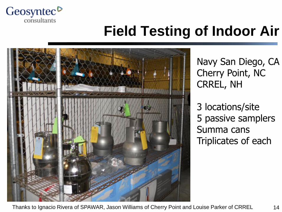
Field Testing of Indoor Air
Thanks to Ignacio Rivera of SPAWAR, Jason Williams of Cherry Point and Louise Parker of CRREL
Navy San Diego, CA Cherry Point, NC CRREL, NH 3 locations/site 5 passive samplers Summa cans Triplicates of each

Indoor Air TCE at San Diego
15
Geosyntec C> consultants
~T~1chloroethene
• Summa • WMS (Ano•nrh 74i)
(Activated carbon wafer) 8 ~~ ~~~~~~~~----------~--------~
ATD (Chrornosorb 106)
• Rad iello (Ar.tlvotod dlen>nrn)
• SKC Ultra IChromose,~ 106) ~ 6 ~----~~~~------------------------------~-------------4 .§ Cl :::J_ -c 4 0 :p ell ._ -c a> 2 (.) c 0 u
0
IA-1
Each oor Is an average of the three ~;;;Jtnpl ~t:i o:>l ect~d at that lot.:.:1Uon
IA-2
Sample Location IA-3 Average

Indoor Air at CRREL
16
All passive sampler results were within 2X of Summa canister data for TCE

Indoor Air VOCs at Cherry Point
17
R²=0.93704
R²=0.97432
R²=0.86277
R²=0.78629
R²=0.94646
0.01
0.1
1
10
100
0.01 0.1 1 10 100
SummaCanisterConcentra on(µg/m3)
WMS
3MOVM
ATD
RAD
SKC
Linear(WMS)
Linear(3MOVM)
Linear(ATD)
Linear(RAD)
Linear(SKC)
Linear(1:1)
Linear(+50%)
Linear(-50%)
Linear(+2x)
Linear(-2x)
PassiveSamplerConcentra
on(µg/
m3)
PassiveSamplervs.SummaCanisterforIndoorAir
Broader range (>100X), but still almost all passive data are within 2X of Summa canisters

High Concentration Lab Tests
(To mimic soil gas conditions)

High Concentration Lab Tests
19
Geosyntec C> consultants

High Concentrations Test Results
0.0
0.2
0.4
0.6
0.8
1.0
1.2
1.4
1.6
1.8
WMS ATD Radiello 3M OVM SKC
C/C
o
Sampler Type
Normalized Concentrations (10 ppm Test)
MEK
n-Hexane
12DCA
111TCA
Benzene
CT
TCE
PCE
124TMB
+/- 25%
+25%
-25%

Sub-Slab – Navy San Diego
Sub-slab samples only
Fully-passive and with PID purging (flow-through)
Starvation proportional to uptake rate
Less starvation for semi-passive samples

Modified Uptake Rates
22
ATD Tube & Pinhole Cap
SKC Ultra II and 12-hole Cap
Lower uptake rate = less starvation

Sorbent Selection
Geosyntec e> consultants
Carbopack B ~~~~- t:o ..... o IIIOUJ , ........ _, .. \ .. ,
O.ot,lololll<)-. T~"w·••- · •fl"l 'C
§ SUPELCO
Carbopack X !o,;o1(10'•to.: uco• ,_,
11 . .... ., ... _ u ... ,., Ql.e('OI'II.~T'""f.._.,,_, la'C
§ SUPELCO

Soil Gas @ 12 ft – Hill AFB
6 probes -12 ft deep
Latin Square Design
1 to 12 day exposures
Co Measured using
combination of
Summa and Hapsite
GC/MS
Negative bias for long duration with ATD-Tenax
Negative bias for high uptake rate (Radiello)
Otherwise, encouraging results for TCE and DCE

Flow-Through Cell – CRREL
Flow-through cell to avoid starvation by design
No starvation for high-uptake rate samplers
Negative bias only for short duration/low-flow
(insufficient purging)
+25%
-25%
Geosyntec C> consultants
CRREL Sub-Slab Flow-Through Coli- TCE
Uo::o.l••••...,., ... ,, ~-o,.:lif:•J,U
-
.,_ ~ -L~ il ~
• .,.., .. 1(((13)
I .........

Soil Vapor Sampling – NAS JAX
Probes to 3-4 feet deep, exposure durations of 20, 40 and 60 minutes
Strong correlations, regression slopes all near 1.0
Geosyntec C> consultants
"' ' ·-'!' ""· < • ·c
~ • < 8 • ~ ~ <, • '"" ·' ~ •
10 JO: ....
• \\'r..t:<f'H
a O~'M
6 4TO
8 !lC
t-- o.lce" !l:ll
Llr~~~ j'<'.lrJSPH)
li: .. . .. , ... ,1--·Li'"' 10'/r.tJ
R,l:().~.SS~ l1re:1t !P.IC)
II:: ··'"'"I····· Lil'~lll !*C)
;r.,.~, I '•".t»\ 'I
1:,000

Passive Sub-Slab – NAS JAX
Limited to 1-inch diameter or less – Low-Uptake Rate Samplers
Geosyntec C> consultants
100•0)3 ,----,P=-a-,-,'"iv-e"'s'"a-m- p'"le_r_vs_. ""su_m_m_a-..,C'""a-n'"is"'"te-r--=co_m_p_a-r'"is_o_n---,~~--,
r
i c 8 g s " c s 1,(100 ' .. n
li ~
~ >i II
1000
f..l • O.!J:ilD - U'Ie¥('1/f'ISI
ll ' • 0.8.3$76 --t.ho:.lf ~TO f1.1bo:l
t. ' a 0 71)"?1!--U"e,r(lb:did ol
--uwx( l : t)

Temporary Passive - NAS JAX
0
0.5
1
1.5
2
2.5
3
cDCE tDCE PCE TCE
C/C
o
Compound Type
WMS-PH Samples vs Summa Canisters
Exposure 1.7hr
Exposure 3.2
Exposure 8.5hr
Exposure 15.5hr
Exposure 18.0hr
Exposure 18.9hr
+/- 25%
+25%
-25%

Overall Correlation between
Passive and Active Samplers
29
Strong correlation to conventional samples over 6+ orders of magnitude Quantitative results for soil vapor (a breakthrough)
I
Geosyntec C> consultants
] , ~ -• -• l ~ -l • • 1
•
I • • u • -- .. 1 • .. · - -C•~IMioo$otl_c.orl_l~_
---
........ .... _ ..
- -A
I I i
/ · - /.
7 ' ~
? ' ·---~ ' -~ -~ '
•
i •
•
/ --
- "" -· l --· • j " • •• l
I --------.. -.. .. • - - - - -c.c .... ~ ",,."'"-lUI"'!
- "'llldlo
-1
• -I - • i -L • • l
I --•~»-""
! ----. L
••
•• .. • - - ·- - -c-- -· .... -a.,.-1,.'-.ll

30
Maybe we don’t need to be using so many Summa Canisters

Cost Comparison
31
Simple comparison: 6 indoor samples 2 outdoor samples 6 sub-slab samples
Ballpark 50% cost for passive samplers versus Summa cans (even with some side-by-side Summa cans for benchmarking, you can still save a lot of money)

Case Study – Air Force Base
TCE concentrations in Area of Interest:
Groundwater up to 100,000 ug/L
Soil Vapor up to 6,000,000 ug/m3
Used Waterloo Membrane Samplers (4
weeks)
No VOCs above RBSLs or ambient background
Open Bay Doors – huge ventilation rate
Screen out, or reduce to low priority for VI
Even if there is no significant risk, it still needs to be documented Regulators & occupants often prefer indoor air data

High Purge Volume Sampling
Fan or Vacuum Bleed Valve Sample Port Vacuum Gauge Cored Hole Lung Box

PID Reading vs Volume Purged
Infer concentrations versus distance based on C versus V trend Minimize risk of missing a localized “hot spot”
Volume Purged
PID
Readin
g
steady

Note “Block F”
Semi-conductor manufacturer,
roughly 100,000 ft2 (i.e. 100
sub-slab samples?)
Conducted 12 HPV Tests
2 in soil gas probes
7 in sub-slab probes
3 in monitoring wells
High Purge Volume
(HPV) Testing

36
--•• --
I
~b'omJoan9 '

37
I
L

38
PID versus Volume Purged
“Block F”
What happened to all the spatial variability in sub-slab data?

Pressure Transducers / Data Loggers
In just a few minutes, you’ve got “pump-test” data
Geosyntec C> consultants

Drawdown and Recovery
Geosyntec C> consultants
U.l CXJO
0.0000
200 600 !000 1400 1600 1800 ~
= E -0.1000 " 0 "' ~ - -0.2000 "' ;. ... 0
~ -= -0.3000 .... = -E " " " "' :>
-Ci .41100
-0.5000
-0.6000 Time (seconds)

Leaky Aquifer Model for SSD
FLOOR SLAB
GRANULAR
FILL LAYER
Top of Native Soil
native soil less permeable than granular fill
Hantush & Jacob, 1955
Thrupp, G.A., Gallinatti, J.D., Johnson, K.A., 1996, “Tools to Improve Models for Design and Assessment of Soil Vapor Extraction Systems”, in Subsurface Fluid-flow (Groundwater and Vadose Zone) Modeling, ASTM STP 1288, Joseph D. Ritchey and James O. Rambaugh, Eds., American Society for Testing and Materials, Philadelphia. pp 268-2 Massman, J. W., 1989, “Applying Groundwater Flow Models to Vapor Extraction System Design,” J. of Environmental Engineering, Vol. 115, No. 1, pp. 129-149.

Leaky Aquifer Type-Curves
Bear, J., 1979, Hydraulics of Groundwater, McGraw-Hill, New York, 560 pp.
r/B = 0.1
r/B = 0.2
r/B = 1.5
r/B = 1.0
r/B = 1.5
r/B = 2.0
Geosyntec C> consultants
1.0 -.-----------------------:::::~ ---'C'
i 0 ~ ..c. 0.1 (J c::
Confined Type-Curve ---............ _ .. .,.--~, .. -
Increasing Infiltration
1 10 100 1000
Time (minutes)

Hantush Jacob Model Fit Vacuum measurements 6 feet from extraction point
Time (seconds)
Dra
wdow
n (
feet
of
air h
ead)
Very good fit between model and vacuum vs time data
Curve fitting yields T and r/B values
B = 14 ft

Floor Slab Conductivity
K’ = vertical pneumatic conductivity of the floor slab [L/t] b’ = floor slab thickness [L], easily measured T = transmissivity [L2/t], a direct output of the model B = leakance [L], also output from the model Therefore, if you know b’ (slab thickness), you can calculate the vertical pneumatic conductivity of the slab
K’ = T b’ B2

Calculations
(r/B)KT π2
QVacuum 0
w (r/B)KB
1
n b π2
Q)( 1
wrv
Portion of flow from leakage Portion of flow from below the slab
(r/B)KB
r)(1
wQrQ

Summary
Point measurements in space and time are variable
We assess risks for a 25 to 30-year exposure scenario
Data should be representative and cost effective
Long-term samples minimize temporal variability
Large volume samples minimize spatial variability
Easy to add pneumatic testing and get design data
Passive sampling can now give quantitative soil vapor data
Regulatory acceptance is progressing
46

Conventional Radius of Influence
ROI about 40 feet
Case Study: 100,000 ft2 commercial building, slab-on-grade

48
Geosyntec C> consultants