Managing Interconnect Resources Embedded SLIP Tutorial Phillip Christie.
51
Managing Interconnect Resources Embedded SLIP Tutorial Phillip Christie
-
date post
21-Dec-2015 -
Category
Documents
-
view
231 -
download
4
Transcript of Managing Interconnect Resources Embedded SLIP Tutorial Phillip Christie.
Managing Interconnect ResourcesEmbedded SLIP Tutorial
Phillip Christie
Overview
• Performance model• Netlists and signatures• Partitioning and placement• Rent exponents• What do you want to model today?
2
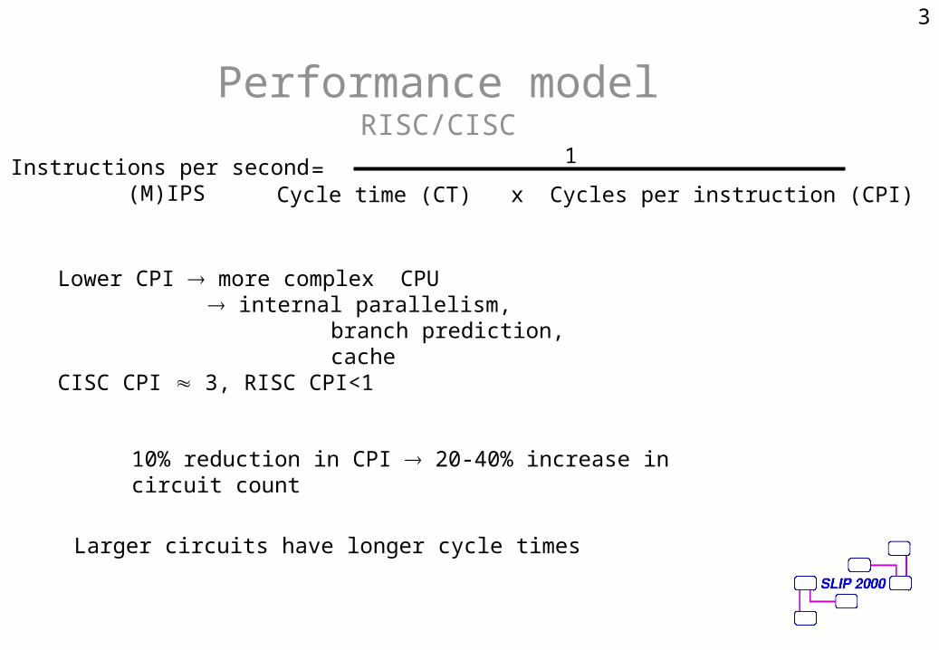
Performance modelRISC/CISC
Cycle time (CT) x Cycles per instruction (CPI)
1Instructions per second (M)IPS
=
Lower CPI more complex CPU internal parallelism,
branch prediction, cacheCISC CPI 3, RISC CPI<1
10% reduction in CPI 20-40% increase in circuit count
Larger circuits have longer cycle times
3

Performance model Logic
CL
CL CL CL
Pipelining CL
CL
CL
CL
Parallelism
Logic Depth
4
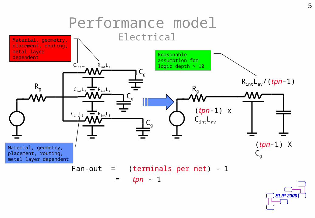
Performance model Electrical
RintL1
RintL2
RintL3
Cg
Rg
Cg
Cg
CintL1
CintL2
CintL3
Rg
RintLav/(tpn-1)
(tpn-1) x CintLav
(tpn-1) X Cg
Fan-out = (terminals per net) - 1
= tpn - 1
Material, geometry, placement, routing, metal layer dependent
Material, geometry, placement, routing, metal layer dependent
Reasonable assumption for logic depth > 10
5
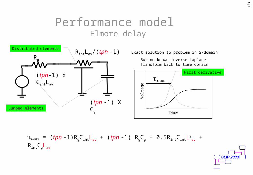
Performance model Elmore delay
Rg
RintLav/(tpn -1)
(tpn-1) x CintLav
(tpn -1) X Cg
0-50% = (tpn -1)RgCintLav + (tpn -1) RgCg + 0.5RintCintL2av + RintCgLav
Lumped elements
Distributed elementsExact solution to problem in S-domain
But no known inverse Laplace Transform back to time domain
Volt
age
Time
First derivative
0-50%
6
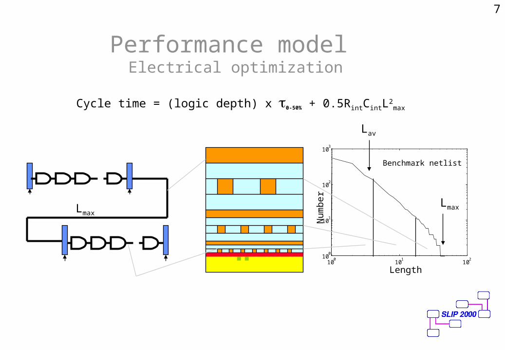
Performance model Electrical optimization
Cycle time = (logic depth) x 0-50% + 0.5RintCintL2max
Lmax
Num
ber
100
101
10210
0
101
102
103
Length
Lav
Lmax
Benchmark netlist
7

Performance model Interconnect optimization
Basic cycle time models provide insight into the complex interactions which determine cycle time.
Modelling process can also be used to optimise power dissipation in the interconnect
8
Performance model Predictive capability
• How do we know if benchmark is good?• Is geometry optimization sensitive to
netlist signature?• What if layout tools change?• What if we wish to analyse performance
of a netlist that does not yet exist?
9

Netlists and signaturesformats
Node list
P1 N1P2 N4P3 N5C0 N1 N2C1 N1 N3C2 N2 N3 N4C3 N2 N3 N5
P1C3
C1
C0
C2
P2
P3
N1
N2
N3
N4
N5
Net list
N1 P1 C0 C1N2 C0 C2 C3N3 C1 C2 C3N4 C2 P2N5 P3C3
Net 2 has 3 terminals per net (tpn)
Cell 3 has 3 nets per cell (npc)
10

Netlists and signaturesterminals per net (tpn)
0 5 10 15 20 25 300
50
100
150
200
250
300
Terminals per net (tpn)
Nu
mber
of
nets
ppone, 25-Feb-2000, <tpn>=2.8686
0 5 10 15 20 250
1000
2000
3000
4000
5000
6000
7000
8000
9000
Terminals per net (tpn)
Nu
mb
er
of
nets
ibm01, 25-Feb-2000, <tpn>=3.5834
11

Netlists and signaturesNets per cell (npc)
1 2 3 4 5 6 7 8 9 1011121314150
50
100
150
200
250
Nets per cell (npc)
Nu
mber
of
nets
ppone, 25-Feb-2000, <npc>=3.6115
1 2 3 4 5 6 7 8 9 1011121314150
500
1000
1500
2000
2500
3000
3500
4000
Nets per cell (npc)
Nu
mber
of
nets
ibm01, 25-Feb-2000, <npc>=4.0237
12

Netlists and signaturesTerminal counting
1 2 3 4 5 6 70
1
2
3
4
5
6
Number of cells
Num
ber
of
term
inals
Example netlist 29-Feb-2000
13

Netlists and signaturesRent’s rule
C
T
CC
TT
If an additional C cells are added, what is the increase in terminals T? In the absence of any other information we might guess that
But this is an overestimate since many of these T terminals may already connect into larger red structure and so do not contribute to the total.
We introduce a factor (0 < <1) which indicates how self connected the netlist is
CC
TT
C
dC
T
dT
Or, if C, T are small compared with C and T
Which may be solved to yieldCnpcT
Where <npc> is the average number of nets per cell, and is generated as a constant of integration
Statistically homogenous system
T
C
14
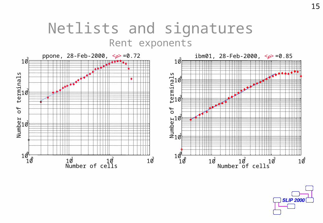
Netlists and signaturesRent exponents
100
101
102
10310
0
101
102
103
Number of cells
Num
ber
of
term
inals
ppone, 28-Feb-2000, <> =0.72
100
101
102
103
10410
0
101
102
103
104
105
Number of cellsN
um
ber
of
term
inals
ibm01, 28-Feb-2000, <> =0.85
15
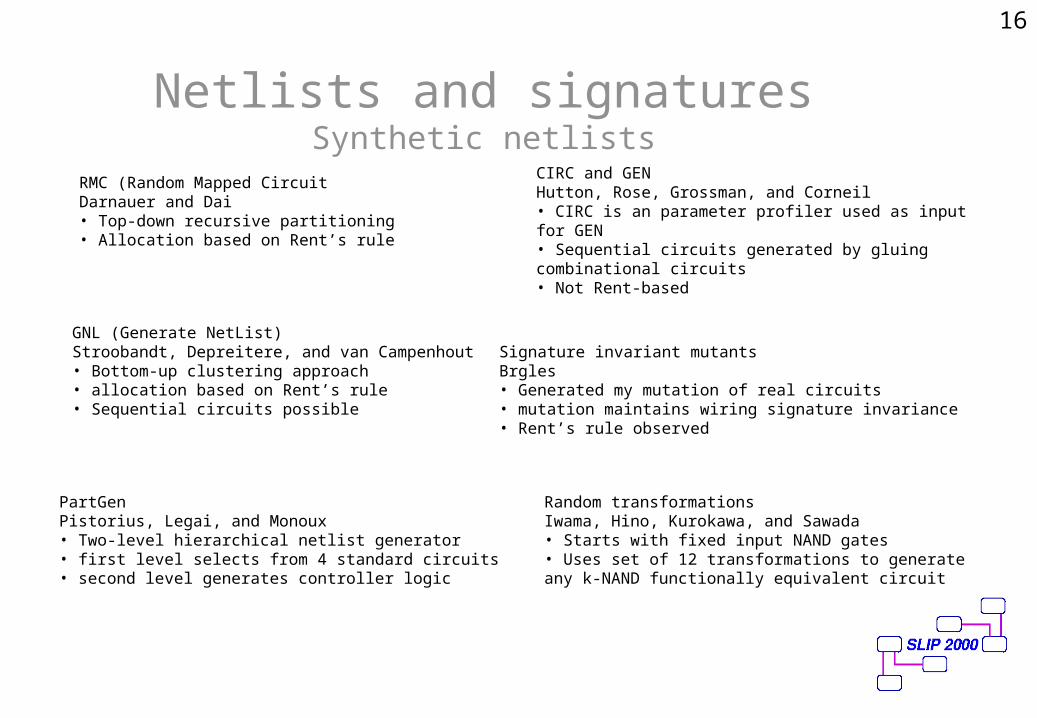
Netlists and signaturesSynthetic netlists
RMC (Random Mapped CircuitDarnauer and Dai• Top-down recursive partitioning• Allocation based on Rent’s rule
GNL (Generate NetList)Stroobandt, Depreitere, and van Campenhout• Bottom-up clustering approach• allocation based on Rent’s rule• Sequential circuits possible
CIRC and GENHutton, Rose, Grossman, and Corneil• CIRC is an parameter profiler used as input for GEN• Sequential circuits generated by gluing combinational circuits• Not Rent-based
PartGenPistorius, Legai, and Monoux• Two-level hierarchical netlist generator• first level selects from 4 standard circuits• second level generates controller logic
Signature invariant mutantsBrgles• Generated my mutation of real circuits• mutation maintains wiring signature invariance• Rent’s rule observed
Random transformationsIwama, Hino, Kurokawa, and Sawada• Starts with fixed input NAND gates• Uses set of 12 transformations to generate any k-NAND functionally equivalent circuit
16

Netlists and signaturesAutomatic netlist generation-GNL
• Number of logic blocks and number of inputs/outputs specified by user
• Logic blocks are paired and (pseudo)-random connections made between blocks as determined by Rent’s rule.
• Constant ratio of internal to external connections at each level
Generates a guaranteed Rent exponent and a realistic tpn distribution
17

Netlists and signaturesparameter independence
0 5 10 15 20 250
50
100
150
200
250
300
Terminals per net
Nu
mb
er
of
nets
ppone, <npc> =3.6115, <> =0.72
25
0 5 10 15 200
1000
2000
3000
4000
5000
6000
7000
8000
9000
Terminals per net
Nu
mb
er
of
nets
ibm01, <npc> =4.0237, <> =0.85
mmmCnpcmtpn total111)(
Recent paper shows <tpn>, <npc> and <> are not independent
18

Netlists and signaturesSummary
• <tpn> characterizes net fan-out• <npc> characterizes cell fan-out• <> is the Rent exponent whose meaning is open
for discussion.• These parameters may not be independent• What happens when we embed the netlist into a
two-dimensional surface?
19

Partitioning and placementSample calculation
100
101
102
100
101
102
103
Length
Num
ber
100
101
102
103
100
101
102
103
104
Length
Num
ber
of n
ets
ibm01ppone
Partition-based placement
Lav= 4.5
Minimum length placement
Lav= 5.5
Partition-based placement
Lav= 9.8
Minimum length placement
Lav= 6.2
20
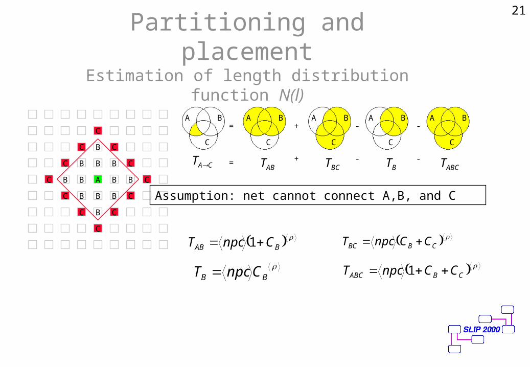
Partitioning and placementEstimation of length distribution function N(l)
B
B
BB
B B
B
A B B
BB
B
C
C
C
C
C
C
C
C
C
C
C
C
C
BA
C
BA
C
BA
C
BA
C
BA= + - -
TAC TAB TBC TB TABC= + - -
Assumption: net cannot connect A,B, and C
BAB CnpcT 1
CBBC CCnpcT
BB CnpcT
CBABC CCnpcT 1
21
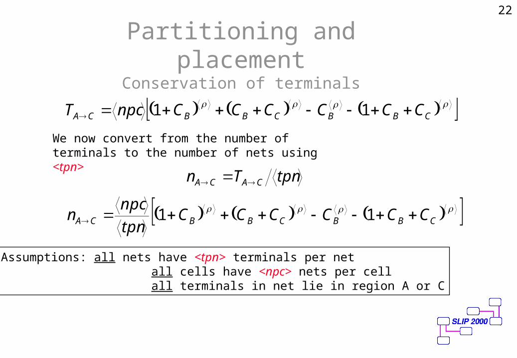
Partitioning and placementConservation of terminals
CBBCBBCA CCCCCCnpcT 11
We now convert from the number of terminals to the number of nets using <tpn>
tpnTn CACA
Assumptions: all nets have <tpn> terminals per net all cells have <npc> nets per cell all terminals in net lie in region A or C
CBBCBBCA CCCCCC
tpn
npcn 11
22

Partitioning and placementEmbedding process (infinite 2D plane)
B
B
BB
B B
B
A B B
BB
B
C
C
C
C
C
C
C
C
C
C
C
C
For cells placed in infinite 2D plane
lCC 4
)1(241
1
lllCl
lB
ppppCA llllllllll
tpn
npcn 4)1(21)1(24)1(2)1(21
23

Partitioning and placementReality check
(1) All cells have <npc> nets per cell(2) All nets have <tpn> terminals per net (3) Net cannot connect A,B, and C(4) All terminals of net lie in region A or C
(2) is only consistent with (3) and (4) if <tpn> = 2, then nAC = n(l) and represents the number of 2-terminal nets of length l associated with a single cell
lllllllllltpn
npcln 4)1(21124)1(2)1(21)(
For <tpn> > 2, n(l) is internally inconsistent
24

Partitioning and placementProbability function (infinite 2D plane)
)()( lrtpn
npcln
We note
1
14)1(21124)1(2)1(21l
llllllllll
And so we can write
Where r(l) is the probability that a cell has a 2-terminal net of length l.
25
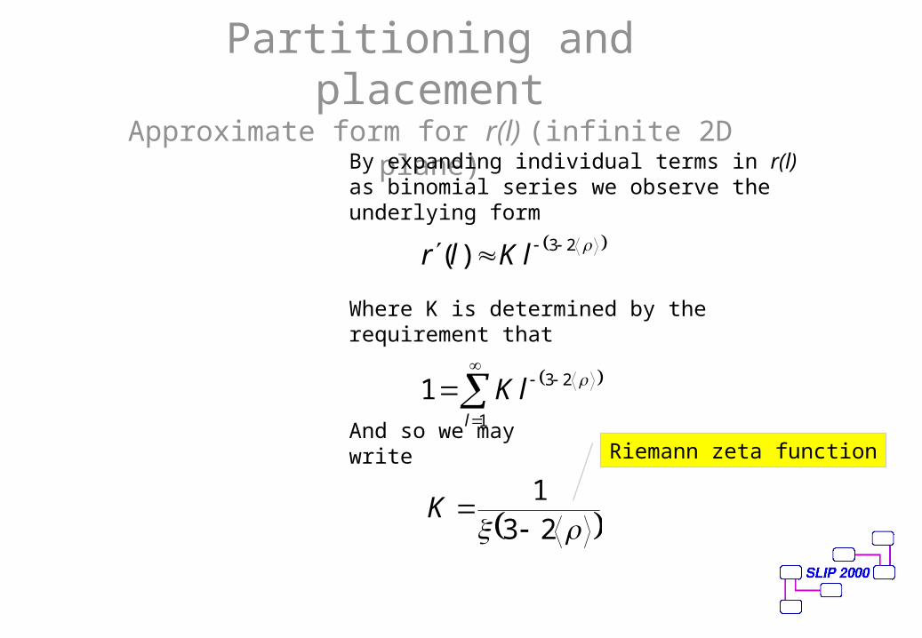
Partitioning and placementApproximate form for r(l) (infinite 2D plane)
By expanding individual terms in r(l) as binomial series we observe the underlying form
23)( lKlr
Where K is determined by the requirement that
1
231l
lK
And so we may write
231
K
Riemann zeta function
100
101
10-3
10-2
10-1
100
Length (gate pitches)
Pro
babi
lity
r(l)
r(l)
26
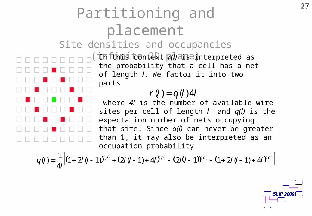
Partitioning and placementSite densities and occupancies (infinite 2D
plane)
llqlr 4)()(
In this context r(l) is interpreted as the probability that a cell has a net of length l. We factor it into two parts
where 4l is the number of available wire sites per cell of length l and q(l) is the expectation number of nets occupying that site. Since q(l) can never be greater than 1, it may also be interpreted as an occupation probability
lllllllllll
lq 4)1(21124)1(2)1(2141
)(
27

Partitioning and placementPlanar model A
L
L
Finite system, Ctot=L2, no edges, approximate form for q(l)
Assume q(l) retains functional form from infinite plane but now use site density function for finite cyclic system and appropriate normalization
)()( lrNlN tot
tottottot CC
tpn
npcN
22)( lLlDa
)()()( lqlDKlr a
L
l
lr2
1
)(1
28
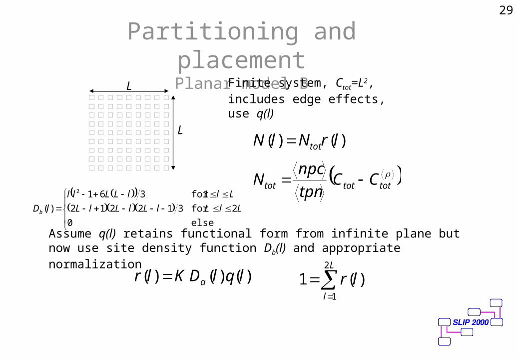
Partitioning and placementPlanar model B
L
L
else0
2for 312212
1for 361
)(
2
LlLlLlLlL
LllLLll
lDb
Finite system, Ctot=L2, includes edge effects, use q(l)
)()( lrNlN tot
tottottot CC
tpn
npcN
Assume q(l) retains functional form from infinite plane but now use site density function Db(l) and appropriate normalization
)()()( lqlDKlr a
L
l
lr2
1
)(1
29

Partitioning and placementPlanar model comparison
100
101
102
100
101
102
103
104
Length
Num
ber
of n
ets
Model A
Model B
Ctot = 1024<tpn> = 2<npc> = 4<> = 0.66
Model A: Lav = 4.53Model B: Lav = 2.27
30
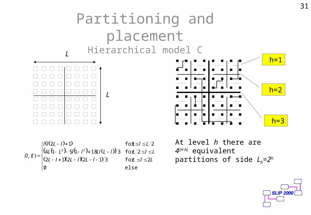
Partitioning and placementHierarchical model C
L
L
else0
2for 312212
2for 3181514
21for 12
)(22
LlLlLlLlL
LlLlLLlllLL
LllLll
lDc
At level h there are 4(H-h) equivalent partitions of side Lh=2h
h=1
h=2
h=3
31

Partitioning and placementRelationship between Model B and C
0 10 20 30 40 50 60 700
0.5
1
1.5
2x 10
4
Length
Nu
mb
er
H
hc
hHb hlDlD
1
),(4)(Dc(l,h)
Db(l)
32

Partitioning and placementIntra-layer model C
),(),( hlrNhlNtoth
)(),(),( lqhlDKhlr c
hL
l
hlr2
1
),(1
As before, within each level
where
Only remaining problem is to estimate number of nets in each level, Nhtot
Net distribution for system is given by sum over hierarchies
H
h
hlNlN1
),()(
33
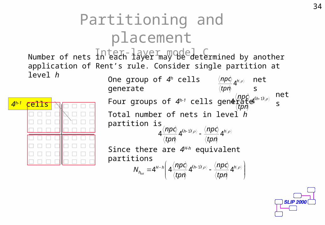
Partitioning and placementInter-layer model C
Number of nets in each layer may be determined by another application of Rent’s rule. Consider single partition at level h
4h-1 cells 144 h
tpn
npc
h
tpn
npc4
Four groups of 4h-1 cells generate
One group of 4h cells generate
hh
tpn
npc
tpn
npc444 1
Total number of nets in level h partition is
Since there are 4H-h equivalent partitions
hhhH
h tpn
npc
tpn
npcN
tot4444 1
nets
nets
34
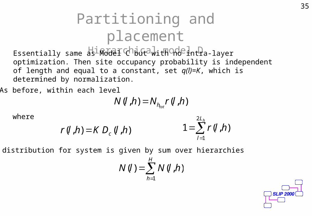
Partitioning and placementHierarchical model D
Essentially same as Model C but with no intra-layer optimization. Then site occupancy probability is independent of length and equal to a constant, set q(l)=K, which is determined by normalization.
As before, within each level
where
),(),( hlrNhlNtoth
hL
l
hlr2
1
),(1),(),( hlDKhlr c
Net distribution for system is given by sum over hierarchies
H
h
hlNlN1
),()(
35
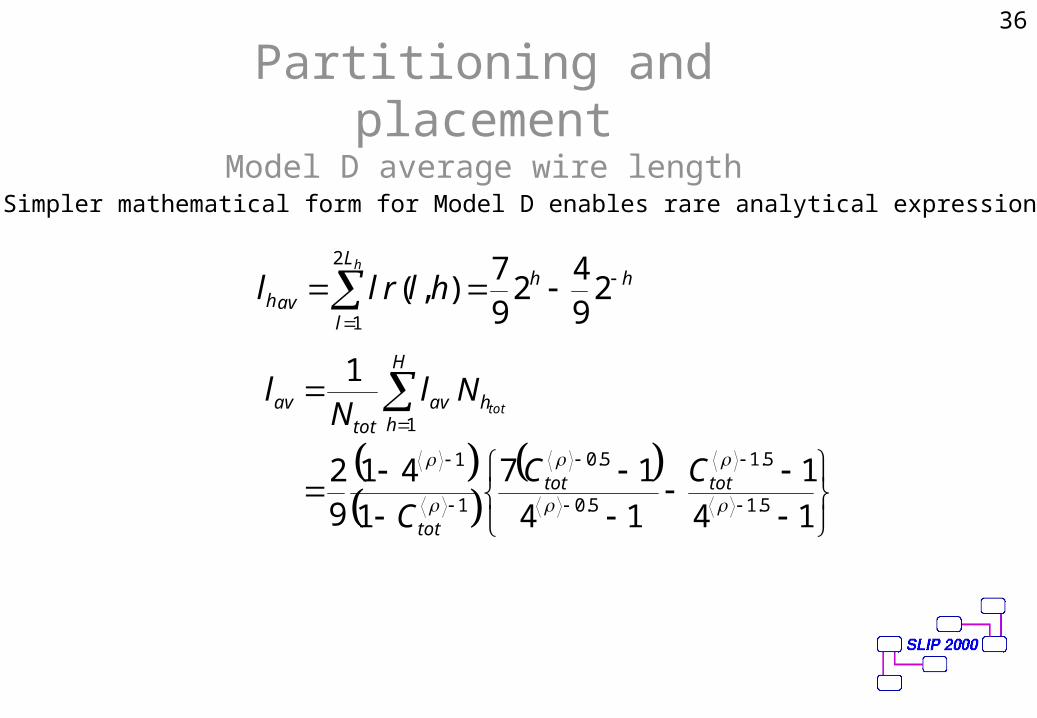
Partitioning and placementModel D average wire length
Simpler mathematical form for Model D enables rare analytical expressions
hhL
lavh
h
hlrll
294
297
),(2
1
14
1
14
17
1
4192
1
5.1
5.1
5.0
5.0
1
1
1
tottot
tot
H
hhav
totav
CC
C
NlN
ltot
36

Partitioning and placementHierarchical model comparison
100
101
102
100
101
102
103
104
Length
Num
ber
Model D
Model C
Ctot = 1024<tpn> = 2<npc> = 4<> = 0.66
Model C: Lav = 2.05Model D: Lav = 5.14
37

Partitioning and placementPlanar and hierarchical model comparison
100
101
102
100
101
102
103
104
LengthN
umbe
r
Model D
Model C
100
101
102
100
101
102
103
104
Length
Num
ber
of n
ets
Model A
Model B
Models B (planar) and C (hierarchical ) are sometimes equivalent
38

Rent exponentsTopology versus Geometry
mmmCnpcmtpn TT pptotal
111)(
The first use of the Rent exponent was to estimate the distribution of m-pin nets
Topological Rent exponent, now written as pT
Topological Rent exponent inappropriate. Define geometrical Rent exponent pG . Measure of placement optimization, not an intrinsic netlist property
GGGG pppp lllllllllll
lq 4)1(21124)1(2)1(2141
)(
But how do we estimate the geometrical Rent exponent?
39
Rent exponentsWiring cell analysis
Let us consider a simple two-level circuit, optimized for placement
With reference to Nhtot from inter-layer model C we note that
For the above example N1tot=11, N2tot=5 and <tpn> =2.0. Therefore
pG =0.431 <npc>1+2=2.0
pG 1 4log
npc tpnN N tpn
Ntot tot
tothh
1 2
1 2
21
2
16 4
or
also
40
G
tot
tot p
h
h
N
N 11 4
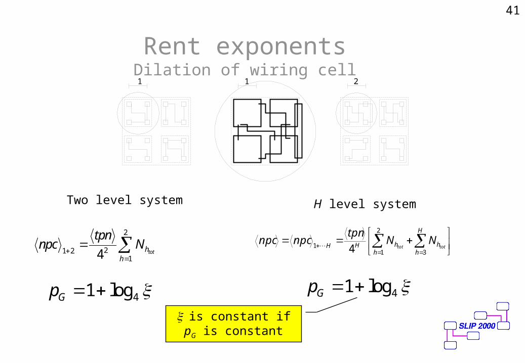
Rent exponentsDilation of wiring cell
1 21
npctpn
Nhh
tot1 2 21
2
4
pG 1 4log pG 1 4log
H level systemTwo level system
is constant if pG is constant
41
H
hh
hhHH tottot
NNtpn
npcnpc3
2
11 4
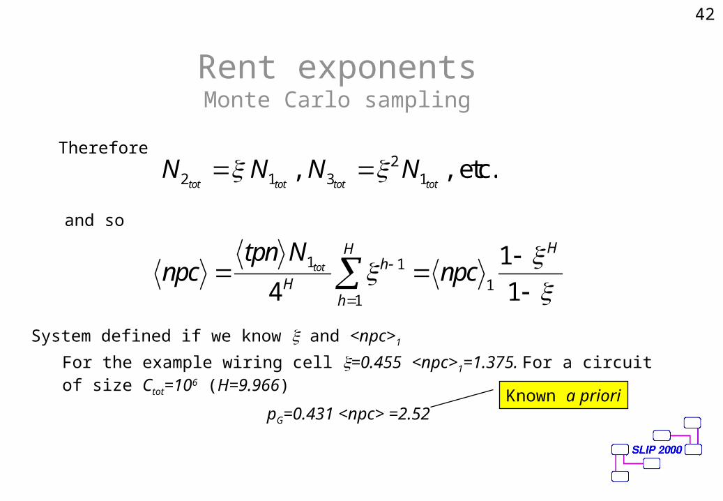
Rent exponentsMonte Carlo sampling
ThereforeN N N N
tot tot tot tot2 1 32
1 , , etc.
npctpn N
npctot
Hh
h
H H
1 1
114
1
1
For the example wiring cell =0.455 <npc>1=1.375. For a circuit of size Ctot=106 (H=9.966)
pG=0.431 <npc> =2.52
and so
System defined if we know and <npc>1
Known a priori
42

Rent exponentsSampling applet
43
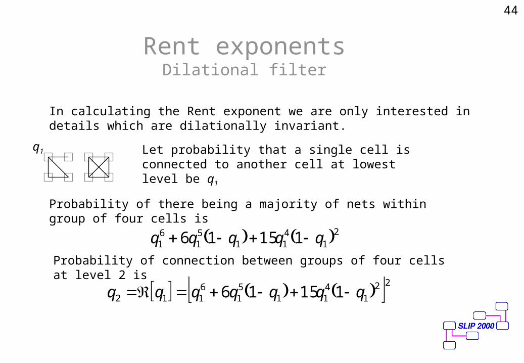
Rent exponentsDilational filter
In calculating the Rent exponent we are only interested in details which are dilationally invariant.
Let probability that a single cell is connected to another cell at lowest level be q1
Probability of there being a majority of nets within group of four cells is
q1
Probability of connection between groups of four cells at level 2 is
44
21
411
51
61 11516 qqqqq
221
411
51
6112 11516 qqqqqqq
Rent exponentsNon-linear functionality
0 0.2 0.4 0.6 0.8 10
0.2
0.4
0.6
0.8
1
q1
q 2
N
N
D
D
q
q
q
q
q
q
tot
tot
tot
tot
2
1
2
1
2
1
2
1
1
1
4 4
npc tpn q1 1
6
4
and <npc> expressed parametrically in terms of q1
45

Rent exponentsTheory versus experiment
MBC algorithm1024 cell netsists
MBC algorithmMonte Carlo Sampling
Majority ruleRenormalization group
46
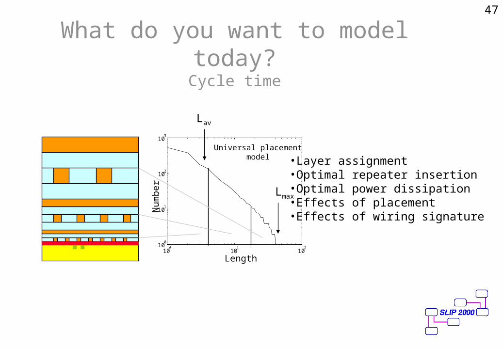
What do you want to model today?Cycle time
47
Num
ber
100
101
10210
0
101
102
103
Length
Lav
Lmax
Universal placementmodel •Layer assignment
•Optimal repeater insertion•Optimal power dissipation•Effects of placement•Effects of wiring signature
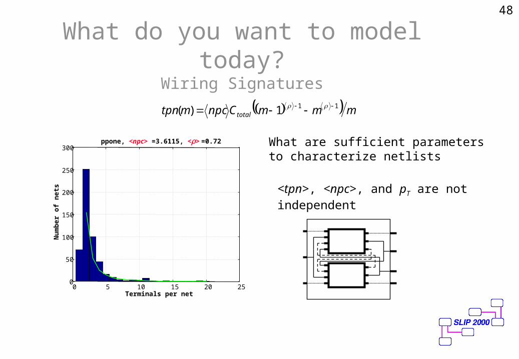
What do you want to model today?
Wiring Signatures
0 5 10 15 20 250
50
100
150
200
250
300
Terminals per net
Nu
mb
er
of
nets
ppone, <npc> =3.6115, <> =0.72
mmmCnpcmtpn total111)(
What are sufficient parameters to characterize netlists
<tpn>, <npc>, and pT are not independent
48

What do you want to model today?
Universal placement model
GG
tot
phphhHh tpn
npc
tpn
npcN 4444 1
H
hch lqhlDNKlN
tot1
)(),()(
GGGG pppp lllllllllll
lq 4)1(21124)1(2)1(2141
)(
B Model 'GG pp
C Model 'GG pp
D Model )(1 KqpG
49

What do you want to model today?
Rent exponents
50

Object oriented approach to system-on-a-chip integration
Extremely difficult to predict interconnect resources required to implement global wiring between inhomogeneous system blocks
What do you want to model today?
Heterogeneous systems
51
Global nets require different modeling techniques