IZA DP No. 738

Managerial Job Assignment and ImperfectCompetition in Asymmetric Equilibrium

Volker Grossmann

March 2003DI

SC

US

SI

ON

PA

PE

R S

ER

IE

S

Forschungsinstitutzur Zukunft der ArbeitInstitute for the Studyof Labor

Managerial Job Assignment and

Imperfect Competition in Asymmetric Equilibrium

Volker Grossmann University of Zurich and IZA Bonn

Discussion Paper No. 738

March 2003

IZA

P.O. Box 7240 D-53072 Bonn

Germany

Tel.: +49-228-3894-0 Fax: +49-228-3894-210

Email: iza@iza.org

This Discussion Paper is issued within the framework of IZA’s research area Mobility and Flexibility of Labor. Any opinions expressed here are those of the author(s) and not those of the institute. Research disseminated by IZA may include views on policy, but the institute itself takes no institutional policy positions. The Institute for the Study of Labor (IZA) in Bonn is a local and virtual international research center and a place of communication between science, politics and business. IZA is an independent, nonprofit limited liability company (Gesellschaft mit beschränkter Haftung) supported by the Deutsche Post AG. The center is associated with the University of Bonn and offers a stimulating research environment through its research networks, research support, and visitors and doctoral programs. IZA engages in (i) original and internationally competitive research in all fields of labor economics, (ii) development of policy concepts, and (iii) dissemination of research results and concepts to the interested public. The current research program deals with (1) mobility and flexibility of labor, (2) internationalization of labor markets, (3) welfare state and labor market, (4) labor markets in transition countries, (5) the future of labor, (6) evaluation of labor market policies and projects and (7) general labor economics. IZA Discussion Papers often represent preliminary work and are circulated to encourage discussion. Citation of such a paper should account for its provisional character. A revised version may be available on the IZA website (www.iza.org) or directly from the author.

IZA Discussion Paper No. 738 March 2003

ABSTRACT

Managerial Job Assignment and Imperfect Competition in Asymmetric Equilibrium�

This paper develops a model with multiple market locations in which the quality of intangible assets of firms, provided by management, determines the firms’ performance. Despite an ex ante symmetry of potential entrants, the equilibrium assignment of heterogeneous managerial skills to firms tends to be asymmetric. This sorting outcome determines both the goods market structure at single locations and the size distribution of firms. Results are consistent with a number of observed patterns regarding the size distribution of firms and establishments, and the relation of firm size to profitability, productivity, managerial skills and manager remuneration. JEL Classification: D40, J31, L16 Keywords: asymmetric equilibrium, firm size, intangible assets, managerial job

assignment Volker Grossmann University of Zurich Socioeconomic Institute Raemistr. 62 CH-8001 Zurich Switzerland Tel.: +41 1 634 22 88 Fax: +41 1 634 49 96 Email: volker.grossmann@wwi.unizh.ch

� I am grateful to Johannes Binswanger and Josef Falkinger for detailed comments on previous versions of the paper. Moreover, I am indebted for helpful discussions to Tomer Blumkin, Armin Falk, Gilles Saint-Paul, John Sutton, and seminar participants at the University of Zurich and the Econometric Society European Meeting (ESEM) 2002, held in Venice.

1 Introduction

In the industrialized world, intangible assets like organizational know-how, product

design, trademarks and the internal human capital stock are key factors for the

performance of Þrms. Development of intangible assets, e.g., through product de-

sign, organization of production, marketing and informal training of workers, is the

responsibility of the management of a Þrm and gives rise to economies of scale and

imperfect product markets. These observations suggest that there are important

interactions between product market characteristics and the market for managerial

skills. This paper develops a model which analyzes this interaction. By doing so, the

model is capable to explain empirical regularities regarding the size distribution of

Þrms and establishments, and the relation of Þrm size to proÞtability, productivity,

managerial skills and manager remuneration in a uniÞed framework.

The basic hypothesis of the model is that the quality of intangible assets depends

on an (aggregate) index of managerial skills in Þrms.1 Firms set up head departments

by hiring managers from a heterogeneous distribution of skills. Managerial wage

costs for the development of intangible assets are endogenous and treated as sunk

costs at the product market competition stage. There is free entry of Þrms into the

economy and all potential entrants are ex ante identical. The economy has multiple

market locations and entry into single markets is a prerequisite to participate in local

product market competition. After the hiring of managers, Þrms choose the market

range in which they operate, i.e., their number of plants or branches. Intangible

assets are geographically non-rival, i.e., are common assets for Þrms in any market

location they are active (e.g., Markusen (1995), Wong (1995)). However, there

are �Coasian� diseconomies of scale in coordinating and governing single plants or

branches (e.g., Williamson (1975), Porter (1986)).

According to the model, product markets and the market for managerial skills

interact in the following way. On the one hand, the nature of product market1Also quantitatively, managerial employment is important. According to Berman, Bound and

Grilichis (1994, Tab. I), in U.S. manufacturing the employment share in managerial occupations

was 10.9 percent in 1987, with rising tendency. See also Grossmann (2002).

2

competition determines, for a given wage structure, the incentive of Þrms to hire

managers with high skills. On the other hand, the sorting of managerial skills in

Þrms determines both the goods market structure at single locations and the size

distribution of Þrms. It is shown under which product market characteristics and

technological conditions an asymmetric equilibrium assignment of managers to Þrms

is obtained despite an ex ante symmetry of potential entrants.2

After analyzing the general structure of the model, both the results and the

equilibrium concept are illustrated by specifying the nature of product market com-

petition. In these examples, the quality of intangible assets is reßected by the

perceived quality of goods or unit production costs. First, it is shown that under

monopolistic competition à la Dixit and Stiglitz (1977), Þrms are completely segre-

gated by managerial skill if the price elasticity of demand is sufficiently high, i.e., if

product market competition is intense. The underlying reason is that, in this case,

small differences in the quality of intangible assets become magniÞed in large proÞt

differences, with greater magniÞcation for higher quality levels. All other things

equal, this leads to high incentives for Þrms to hire good managers, implying a

symmetry-breaking feedback effect on the assignment of managerial skills to Þrms.

This driving force towards asymmetry of managerial job assignment is also at work

in a second example, which examines monopolistic competition under linear demand

schedules (Ottaviano and Thisse (1999)).

The literature on assignment of heterogeneous workers to Þrms has recently

gained renewed interest (e.g., Kremer (1993), Kremer and Maskin (1996), Saint-2Related literature usually predicts that symmetry of potential entrants leads to symmetric

free-entry equilibria. For instance, in standard versions of �love of variety� models of monopolistic

competition (Spence (1976), Dixit and Stiglitz (1977)), �ideal variety� models (Lancaster (1979),

Helpman (1981)) or �location� (spatial) models (Hotelling (1929), Salop (1979)) the number of

active Þrms is determined by some exogenous entry costs and Þrms are ex post identical. An

exception is Fishman and Rob (1999) who study a model with a given number of initially identical

Þrms, in which cost shocks generate an asymmetric steady-state equilibrium. Another strand of

literature are models of industry dynamics, which usually assume ex ante heterogeneous Þrms

(e.g., Jovanovic (1982), Athey and Schmutzler (2001)). The present model may be viewed as

complementary to this literature, explaining why Þrms differ in the Þrst place.

3

Paul (2001), Shimer and Smith (2000), Shimer (2001), Prat (2002)). This literature

highlights the role of technological complementarity and spillovers among workers

for a segregation of Þrms by their workers� skill. (For a comprehensive review of

the less recent literature on job assignment, see Sattinger (1993).) In contrast,

this paper derives asymmetric equilibria with respect to the sorting of skills from

product market characteristics, by accounting for the role of intangible assets for

the performance of Þrms.

The work of Rosen (1982) and Saint-Paul (2001) are most closely related to the

present analysis. Saint-Paul (2001) shows that, by allowing for intra-Þrm spillovers

when output of a homogenous good is a function of an aggregate skill index, typi-

cally, the equilibrium assignment of workers is segregated and the wage distribution

skewed to the right. He applies his model to analyze the impact of new information

technology on segmentation and wage inequality. Thus, his focus is very different

from the present multi-market context in which managerial quality is the key to

create valuable intangible assets and the sorting equilibrium depends on product

market characteristics. Rosen (1982) examines the relationship between Þrm size,

managerial job assignment and managerial wages by focussing on the supervisory

role of management. In his analysis, good managers sort in large Þrms and receive

high rewards because of a technological complementarity between supervising skills

and the span of control. In contrast, in the present analysis, for Þrms to be large in

the Þrst place they have to attract good managers who create valuable intangible

assets. Moreover, the present paper also studies the number of establishments as

measure for Þrm size, in addition to output, sales or employment.

Results are consistent with the following patterns which are discussed in more

detail at the end of this paper. (i) The size distribution of Þrms and plants within in-

dustries is highly skewed to the right (e.g., Sutton (1997)); (ii) both larger Þrms and

Þrms with higher market shares are more proÞtable (e.g., Schmalensee, 1989); (iii)

there is a substantial degree of heterogeneity among Þrms and establishments with

respect to productivity levels, with larger Þrms and plants being more productive

(e.g., Bartelsman and Doms (2000)); (iv) larger Þrms employ better workers (e.g.,

4

Troske (1999)), and, particularly, average managerial skill levels substantially dif-

fer across Þrms (e.g., O�Shaughnessy, Levine and Capelli (2001)); Þnally, (v) larger

Þrms pay substantially higher managerial wages (e.g., Conyon and Murphy (2000)).

The paper is organized as follows. In section 2, the model is presented and its

crucial assumptions are discussed. Section 3 deÞnes the equilibrium and character-

izes market ranges, proÞts, the assignment of managers and the measure of Þrms

in equilibrium. Section 4 illustrates both the results and the equilibrium concept

by specifying the nature of imperfect competition in the multiple goods markets.

Section 5 shows how the results derived from the model relate to the observed pat-

terns (i)-(v) above. Section 6 summarizes the main results. All proofs and extensive

derivations are relegated to an appendix.

2 The Model

This section presents the model and discusses its main assumptions.

2.1 Set Up

Firms are characterized by intangible assets which affect the Þrms� productivity

or (perceived) product quality, respectively. There is a large number of potential

entrants in the economy and entry is free. Let I = [0, I] be the set of Þrms whichactually enter. Firms are proÞt-maximizers.

Labor supply is inelastic and normalized to unity. Workers differ in their abil-

ity h to develop intangible assets, called managerial skill level. Let g(h) be the

mass function of the distribution of skill supply, with support being the set H =

{h0, h1, ..., hK}, 0 ≤ h0 < h1 < ... < hK < ∞. There exists an outside earningsoption W̄ ≥ 0 for types when not being assigned as manager, i.e., with respect to allnon-managerial tasks, labor is homogenous (see, e.g., Lucas (1978)). In the general

equilibrium examples of section 4, W̄ is the wage rate for production workers. Firms

take wages w(h), h ∈ H, as given; there is a Walrasian auctioneer in the labor mar-ket, implementing a wage schedule which fulÞlls equilibrium conditions as deÞned

5

in section 3.3 below (see DeÞnition 2). Workers seek the highest wage.

Firms may (endogenously) differ in a single parameter αi, i ∈ I, called quality ofintangible assets. Intangible assets are created in the Þrms� head departments which

consist of an exogenous mass (�size�) s of managerial workers, with 0 < s ≤ g(h)

for all h ∈ H. The quality index αi is determined by the average managerial skilllevel in the head department of Þrm i, denoted by h̄i ∈ H = [h0, hK ]. Formally, let

a : H → R+ be a strictly monotonic increasing and twice continuously differentiable

function, so that3

αi = a(h̄i). (1)

There is a continuum of market locations (�markets�), indexed by m, which are

represented as points in the unit interval [0, 1]. In order to produce and sell products

in a single market, Þrms have to incur set up costs, e.g., for opening up a plant or

branch, introducing a marketing campaign at a location or costs associated with red

tape. It is assumed that these costs only depend on the measure of markets in which

a Þrm decides to operate, called market range. Formally, let Mi ⊆ [0, 1] be the setof markets in which Þrm i ∈ I is active and let qi be the Lebesgue measure of Mi.

(It is assumed that Mi ∈M, where M is the σ-algebra of Borel sets for the unit

interval.) Firm i�s total set up costs are given by Q(qi), where Q : [0, 1] → R+ is

a monotonic increasing, convex and twice continuously differentiable function with

Q(0) = 0.

Let α,M and q denote mappings which assign to each Þrm i a quality of intan-

gible assets αi, a set of markets Mi in which the Þrm is active and a corresponding

market range qi, respectively, i ∈ I. The timing of events evolves according to thefollowing stages, with decisions at each stage made simultaneously by Þrms.

� At stage 1, each Þrm i ∈ I creates intangible assets by hiring managers from3The size s of head departments could be treated as choice variable of Þrms by replacing (1) by

αi = b(h̄i, s), as long as b(·) is not ever increasing in s (holding h̄i constant). (Such a limitation ofsize advantages can be justiÞed by internal coordination problems which imply that a Þrm�s head

department has an optimal size.) This would not alter the main conclusions of this paper, but

would considerably complicate the analysis. For simplicity, s is exogenous here.

6

the set H, which determines α, according to equation (1). Wage costs formanagers are sunk at later stages.

� At stage 2, Þrms decide in which markets to be active, i.e., each Þrm i ∈ Ichooses a set Mi ∈M, which determinesM and q, respectively.

� At stage 3, Þrms enter product market competition.

The analysis is not restricted to a particular type of imperfect competition model

but generally applies to any form of imperfect product market competition in which

intangible assets matter for the performance of Þrms. The role of intangible assets

for the proÞts of Þrms at stage 3 is speciÞed as follows. Denote proÞt realizations

of Þrm i from product market competition at stage 3 in market m by πi,m. The

mapping M, which assigns a set of markets Mi to each Þrm i ∈ I, determines foreach m ∈ [0, 1] the set Nm := {i ∈ I |m ∈Mi} of Þrms operating in market m.If Þrm i does not enter market m, proÞts at stage 3 in this market are zero, i.e.,

πi,m = 0 if i /∈ Nm. If i ∈ Nm, πi,m depends on the Þrm�s strength αi and on the

competitive pressure exerted by its rivals.

A higher quality αi raises πi,m in any market m ∈Mi (in which Þrm i is active)

similarly. This reßects the idea that intangible assets are geographical non-rival

(as discussed in section 2.2). Competitive pressure in a market m depends on the

strengths of rivals αj, j ∈ Nm, j 6= i. Thus, generally, proÞts at stage 3 in each

market m depend on α, i.e., on the quality levels of intangible assets developed at

stage 1, and on the mappings M, q, resulting from the Þrms� decisions at stage 2

about which and how many markets to enter. The analysis focusses on (equilibrium)

situations in which, given α, for any q, the proÞt-maximizing choices of market sets

Mi at stage 2 are such that each Þrm earns the same proÞt at stage 3 in any market

it is active. More formally, let z ≡ (α,q) denote the mapping which assigns a

pair (αi, qi) to each Þrm i; then, one can write πi,m = π(αi| z) if i ∈ Nm. As a

consequence, the proÞt prospects πi,m faced by a Þrm when deciding about αi and

qi depend on z, not on speciÞc conditions in single markets.4 Since single Þrms4To see this, consider a situation in which competitive pressure differs across markets. Suppose

7

have measure zero, competitive pressure under (α0,q0) is the same as under (α,q)

if α0i = αi and q0i = qi for almost all i ∈ I. Competitive pressure under (α0,q0) is

higher than under (α,q) if α0i ≥ αi and q0i ≥ qi with at least one strict inequality

holding for a positive mass of Þrms i ∈ I. For instance, suppose there are twotypes of Þrms, indexed k = 0, 1, and denote the respective set of Þrms by I0 andI1, respectively; i.e., I = I0 ∪ I1. Let (αi, qi) = (αk, qk) for all i ∈ Ik, k = 0, 1.

Then, for all i ∈ Nm and for all m ∈ [0, 1], πi,m = π(αi| z) is increasing in αi anddecreasing in α0, α1, q0 and q1. (See the examples in section 4.) The following

assumption summarizes the properties of stage 3 equilibria required for the further

analysis.

Assumption 1. For any z = (α,q) there exists a real-valued function π(αi| z),twice continuously differentiable in αi, so that πi,m = π(αi| z) if i ∈ Nm, m ∈[0, 1], and π satisÞes the following properties: (i) ∂π(αi|·)

∂αi> 0; (ii) for z = (α,q),

z0 = (α0,q0), we have π(αi| z) = π(αi| z0) if competitive pressure under (α,q) and(α0,q0) is the same, and π(αi| z) < π(αi| z0) if competitive pressure under (α,q) ishigher than under (α0,q0).

Assumption 1 greatly simpliÞes the analysis, as the decision problem of each Þrm

i ∈ I at stage 2 can be reduced to the choice of market ranges qi rather than thechoice of the entire sets Mi.

Note that the Þrm�s objective function at stage 2 is the sum of Þrm i�s proÞts

at stage 3 over all single markets in which it is active minus total entry costs Q(qi).

As Þrms have a negligible impact, they correctly take z as given at stage 2. Thus,

Assumption 1 implies that, given z, the optimal choice of range qi of a Þrm which

has created a quality of intangible assets αi at stage 1 reads

�q(αi| z) := arg max0≤qi≤1

{qiπ(αi| z)−Q(qi)}. (2)

πi,m > πi,m0 form,m0 ∈Mi, i.e., competitive pressure inm0 is higher than inm. It is assumed that

this cannot hold in an equilibrium because then other Þrms j /∈ Nm should have been induced to

enter market m as well, or Þrm i should have abstained to enter market m0. Thus, in equilibrium,

πi,m = πi,m0 for all m,m0 ∈Mi and for all i ∈ I.

8

2.2 Discussion of the Set Up

Before beginning the equilibrium analysis, let me brießy discuss the set up of the

model.

2.2.1 Managerial Skills and Intangible Assets

It is assumed that intangible assets have to be developed ex ante by managerial la-

bor. For instance, managerial activities include the creation of analytical databases

and intra-Þrm networks, which support the design of products, customer services

and marketing strategies (e.g., Bresnahan (1999)). These tasks affect the (perceived)

quality of goods. Moreover, managerial abilities affect the efficiency of the organi-

zational structure of a Þrm (and, thus, productivity) by developing management

techniques and Þrm-speciÞc human capital (human resource management). Indeed,

empirical evidence suggests that �managerial quality may be an important factor

behind productivity heterogeneity� (Bartelsman and Doms (2000, p. 587)). As the

creation of intangible assets relate to R&D and marketing activities, taking place

prior to product market competition, the model borrows from the IO literature

on investment games by treating corresponding outlays as endogenous sunk costs

(e.g., Shaked and Sutton (1982, 1983), Sutton (1998)). In fact, the present model

allows one to lead back endogenous sunk costs (i.e., managerial wages) to individ-

ual characteristics, accounting for individual heterogeneity and observing resource

constraints.

2.2.2 Geographical Non-rivalry of Intangible Assets

According to the set up of section 2.1, the quality of intangible assets, αi, is Þrm-

speciÞc, rather than plant-speciÞc. This reßects the public good nature of intangible

assets from the perspective of a Þrm (therefore often called �common assets� in the

literature). For instance, αi corresponds to the perceived quality of the product(s)

of Þrm i in any market it chooses to be active. In this case, αi can be interpreted as

the consumers� valuation of Þrm i�s product design(s) or trademark. According to

the literature on the boundaries of (multi-plant) Þrms, intangible assets give rise to

9

ownership advantages.5 In particular, this applies to multinational Þrms. In fact,

Þrms in advertising-intensive industries are more likely to incur foreign direct in-

vestment (Martin (1991)). Moreover, Þrm-speciÞc marketing advantages and trade-

marked goods induce Þrms to �globalize� (e.g., Markusen (1995), Wong (1995)). As

another example, think about αi as productivity of Þrm i. In fact, empirical evi-

dence suggests that productivity in single plants of a Þrm is positively related to the

productivity of the headquarter of this Þrm (Baily, Hulten and Campbell (1992)).

2.2.3 Entry into single markets

According to the model, entry into single markets is a prerequisite to participate

in local product market competition, i.e., Þrms have to open a plant or branch

in order to compete in a speciÞc market.6 Moreover, it is implicitly assumed that

costs of internal transactions are lower than those through market transactions (e.g.,

licensing).7 Q(·) constitutes plant-related sunk costs of Þrms, which have to beincurred in addition to the sunk costs for developing intangible assets. A strictly

convex shape of Q(·) may be justiÞed by logistic problems of Þrms to coordinateand govern single plants or branches. Microeconomic foundations of this assumption

can be found in the literature on internal coordination problems (initiated by Coase

(1937)). Reasons include diseconomies of scale in governing plants (Porter (1986))5The notion of ownership advantages relates to the famousOLI approach (e.g., Dunning (1981)).

On the characteristics of multinational Þrms, see, e.g., Caves (1982) and Morck and Yeung (1992).6For instance, suppose that transport costs are prohibitively high. Examples include service

enterprises like hotel chains, restaurants, banks, airlines or car-rental companies. Moreover, think

about Þrms which have own retail branches (for reasons related to marketing or trademarks) like

Douglas, H&M, IKEA, automobile manufactures, etc.7According to the OLI framework, these two assumptions refer to locational and internal-

ization advantages, respectively. Possible reasons for internalization advantages include agency

problems (Holmström and Milgrom (1991, 1994)), asset speciÞcity (Williamson (1979, 1985) or

non-contractible investments (Grossman and Hart (1986), Hart and Moore (1990)). For a com-

prehensive outline of this literature, see, e.g., Holmström and Roberts (1998). Interestingly, these

authors advise to study common assets as determinant for Þrm boundaries, rather than focussing

on incentive problems only. This is the route taken in the present paper.

10

and costs of bureaucracies (Williamson (1975)).

3 Equilibrium Analysis

This section solves the model by backward induction. The solution characterizes

market ranges, proÞts, the wage structure, the assignment of ability types to Þrms

and the measure of Þrms in an equilibrium.

3.1 Product Market Competition (Stage 3)

Product market competition at stage 3 takes place in each market m ∈ [0, 1] sep-arately, with the set of Þrms I, the qualities of intangible assets α and market

ranges q being already determined. According to Assumption 1, this leads to proÞt

realizations π(αi| z) of a Þrm with strength αi in any market it is active, given the

competitive pressure in the economy under z = (α,q).

3.2 Firms� Choice of Markets (Stage 2)

Optimal behavior of Þrms i ∈ I at stage 2, after creation of intangible assets atstage 1, is given by (2). This implies the following for an equilibrium at stage 2.

DeÞnition 1. (Equilibrium at stage 2). Given the set of Þrms I and themapping α, in an equilibrium, we have �z = (α, �q) with �qi = �q(αi| �z), i ∈ I.

As Þrms take z as given when choosing market ranges, in equilibrium, the optimal

choices of Þrms� market range, given by �q, must be consistent with the resulting

competitive pressure under these optimal choices, i.e., �z = (α, �q).8 Equilibrium

proÞts of a Þrm i ∈ I at stage 2 (�gross proÞts�) then read

Π(αi| �z) := �qiπ(αi| �z)−Q(�qi). (3)8If there is a Þnite set of types of Þrms, as in the examples considered in section 4 below,

the existence of an equilibrium at stage 2 can be established by applying standard Þxed point

theorems. Also note that there may be multiple equilibria, which, however, causes no problems in

our analysis.

11

Applying the Kuhn-Tucker theorem to the maximization problem (2), for all i ∈ I,�qi > 0 fulÞlls the condition

π(αi| �z) ≥ Q0(�qi), (4)

which is binding if �qi < 1.9 Note that �qi < 1 for some i ∈ I only if Q(qi) isstrictly convex for at least some qi ∈ (0, 1]. To see this, suppose to the contrarythat Q(·) would not be strictly convex somewhere. Then π(αi| �z) ≥ Q0(1) and

�qi = 1 would hold. As argued above, a strictly convex shape of set up costs Q(·) is anatural property which reßects diseconomies of scale in coordinating single branches

or plants. The following result emerges. (All results are proven in appendix A.)

Proposition 1. (Market ranges and gross proÞts). For all i ∈ I, (i) ∂�qi∂αi

≥ 0,and (ii) ∂Π(αi|�z)

∂αi> 0.

According to Proposition 1, Þrms with high-quality intangible assets are not

only more proÞtable but, if anything, also have wider market ranges than Þrms with

low-quality intangible assets. If Q(·) is strictly convex, then αi > αj implies �qi > �qjwhenever �qj < 1. Fig. 1 provides a graphical representation of Proposition 1 in this

case. Making use of (3), differences in gross proÞts of Þrms i and j are given by the

shaded area.

<Please insert Figure 1 about here>

The next subsection shows that despite a completely symmetric situation of

potential entrants in the economy, the quality of intangible assets (and, thus, proÞts

as well as, possibly, market ranges) may indeed differ among Þrms in equilibrium, as

an implication of the endogenous sorting of managers into head departments. For

both the intuition of this central result and its implication for the size distribution

of Þrms (discussed in section 5), the following auxiliary result will prove helpful.9Clearly, π(αi| �z) > Q0(0) and thus �qi > 0 in any equilibrium, because otherwise a Þrm would

not enter the economy in the Þrst place. Also note that Π(αi| �z) > 0 for all i ∈ I, according to(3), (4), π(αi| �z) > Q0(0), the convexity of Q(·) and Q(0) = 0.

12

Lemma 1. (Convexity properties). Suppose ∂2π(αi|·)∂α2i

> 0. Then ∂2Π(αi|·)∂α2i

> 0

and, if �qi < 1 and Q000(�qi) ≤ 0, also ∂2�qi∂α2i

> 0.

As will be seen below, strict convexity of reduced-form proÞts at stage 3, π(αi| ·),in αi gives rise to a complete segregation of Þrms by managerial skill.

3.3 Assignment of Managerial Skills (Stage 1)

The Þrms� decision problem at stage 1 is to choose the quality of intangible assets

αi by hiring managers. First, deÞne a class of �assignment functions�

�G := {�g : H→ [0, s] | �g(h) ≤ g(h) for all h ∈ H andXh∈H

�g(h) = s}. (5)

�G describes the feasible hiring policies of a Þrm. At stage 1, each Þrm i ∈ Ichooses an assignment function �gi ∈ �G. Depending on this hiring policy, the average

managerial skill level in Þrm i is given by h̄i = 1s

Ph∈Hh�gi(h). As αi = a(h̄i), the set of

functions �gi ∈ �G, i ∈ I, determines the mapping α. It is helpful to redeÞne proÞtsat stage 2 as function of Þrms� average managerial skill level h̄i, i.e.,

f( h̄i¯̄ ·) := Π(a(h̄i)¯̄ ·). (6)

We are now ready to set up conditions for an equilibrium at stage 1.

DeÞnition 2. (Equilibrium at stage 1). An equilibrium set of assignment

functions �g∗i ∈ �G, i ∈ I, together with a mapping w from H to R+ (wage schedule),

fulÞll the following conditions:

(a) Net proÞts are zero, i.e., for all i ∈ I,

f( h̄∗i¯̄z∗) =

Xh∈Hw(h)�g∗i (h), (7)

where h̄∗i =1s

Ph∈Hh�g∗i (h) and z

∗ = (α∗,q∗), with α∗i = a(h̄∗i ) and q∗i = �q(α∗i | z∗),

i ∈ I.(b) Given z∗, no proÞtable deviation exists, i.e., for all �g0i ∈ �G and for all i ∈ I,

f( h̄0i¯̄z∗) ≤

Xh∈Hw(h)�g0i(h), (8)

13

where h̄0i =1s

Ph∈Hh�g0i(h).

(c) For all h ∈ H, w(h) ≥ W̄ and the following holds: if w(h) > W̄ , thenRi∈I�g∗i (h)di = g(h); if

Ri∈I�g∗i (h)di < g(h), then w(h) = W̄ .

Condition (a) of DeÞnition 2 means that the total wage bill for managers em-

ployed in the head department of a Þrm (i.e., the endogenous sunk cost for the

creation of intangible assets) is equal to its gross proÞt, i.e., net proÞts of all Þrms

are zero in equilibrium. In view of free entry of Þrms into the economy and the com-

petition of Þrms for managerial skills in a perfect labor market, this is a consistent

requirement. With symmetry of potential entrants ex ante, the only possibility for a

Þrm to become more proÞtable (in terms of gross proÞts at stage 2) than other Þrms

is to attract higher-skilled managers on average. Higher gross proÞts of a Þrm just

transmit into a higher average wage per manager of a Þrm. Also note that, in any

equilibrium, Þrms must correctly foresee the competitive pressure z∗, which results

from optimizing behavior of Þrms at stages 1 and 2 (recall DeÞnition 1), as well as

from product market competition at stage 3. Condition (b) reßects that, at stage

1, each Þrm maximizes proÞts taking both competitive pressure z∗ and the wage

schedule w(h), h ∈ H, as given. To see this, note that for any given wage schedulew(h), h ∈ H, no Þrm i wants to deviate from �g∗i ∈ �G (which leads to average skill

h̄∗i ) iff

f( h̄∗i¯̄z∗)−

Xh∈Hw(h)�g∗i (h) ≥ f( h̄0i

¯̄z∗)−

Xh∈Hw(h)�g0i(h) (9)

for all alternative assignment functions �g0i ∈ �G (leading to h̄0i). Inequality (8) then

directly follows from (9) by using the zero-proÞt condition (a). According to condi-

tion (c), all types h ∈ H from the potential pool of managers must at least receive

the outside option W̄ (i.e., the wage rate for non-managerial labor). This implies

f( h̄∗i¯̄z∗) ≥ sW̄ for all i ∈ I, i.e., sunk costs are bounded from below by sW̄ . As

argued in section 3.4, this determines the equilibrium measure of Þrms I∗ under

free-entry. Condition (c) also says that the market for managerial skills must clear

for any type h unless workers are paid their outside option. To see this, suppose

w(h) > W̄ andRi∈I�g∗i (h)di < g(h). This means that there is excess supply for man-

14

agerial positions as workers seek the highest wage. However, this is inconsistent with

a Walrasian equilibrium in the labor market. In contrast, if w(h) = W̄ for some

type h, then this type is indifferent whether or not to be assigned as manager.

Remark 1. DeÞnition 2 extends the equilibrium deÞnition in Saint-Paul (2001)

to analyze the assignment of managerial skills to head departments of Þrms in an

imperfect competition, multi-market context in which managers develop intangi-

ble assets. In contrast, Saint-Paul examines the relationship between technological

change and wage inequality by studying the assignment of production workers to

Þrms under perfect competition. Formally, however, the basic model of Saint-Paul

is a special case of the present framework in which W̄ = 0 (i.e., there is no out-

side wage option) and f( h̄i¯̄ ·) = π(a(h̄i)

¯̄ ·) ≡ a¡h̄i¢for all i ∈ I. That is, in

his model, a(h̄i) is Þrm i�s output of a homogenous (numeraire) good in a single

market when employing s workers with average skill level h̄i. (There are no set up

costs for market entry.) Using this, conditions (a) and (b) of DeÞnition 2 hold in

an analogous way (replacing f( h̄∗i¯̄z∗) by a

¡h̄∗i¢), although wage costs do not have

the interpretation of sunk investments in the set up of Saint-Paul. Moreover, in his

model w(h) > 0(= W̄ ) for all h; i.e., there is full employment of all types, according

to equilibrium condition (c). Correspondingly, the equilibrium measure of Þrms is

given by I∗ = 1/s in this case.10

We are now ready to derive the equilibrium wage structure. DeÞne the sets

Si := {h ∈ H : �g∗i (h) > 0} which contain managerial skill levels (of a total masss of types) hired in equilibrium by i ∈ I. Let S be a mapping which assigns a setSi to each Þrm i, called an equilibrium conÞguration of manager assignments. Also

deÞne S := ∪i∈ISi, i.e., S ⊆ H is the subset of managerial skill levels assigned to

head departments in equilibrium. At stage 1, each Þrm i ∈ I chooses an assignment10As shown in section 3.4 and illustrated in appendix, if W̄ > 0, by contrast, the equilibrium

measure of Þrms I∗ depends on all exogenous factors, i.e., besides on size s of head departments,

on the product demand structure, the nature of product market competition, technologies, and

the distribution of managerial skills.

15

function �gi ∈ �G by maximizing net proÞts f( h̄i¯̄z∗)−P

h∈H�gi(h)w(h), taking z∗ and the

wage schedule w(h) for each type h ∈ H as given. Observing equilibrium conditions

(a)-(c) of DeÞnition 2, we can characterize the equilibrium wage schedule as follows.

Proposition 2. (Wage schedule). In equilibrium,

(i)

w(h) ≥ f( h̄∗i¯̄z∗)

s+∂f( h̄∗i

¯̄z∗)

∂h̄i

h− h̄∗is

(10)

for all h ∈ S, with equality if h ∈ Si, i ∈ I;(ii) there exists hmin ∈ H such that S = {hmin, ..., hK};(iii) w(h) > W̄ for all h > hmin;

(iv) Þnally, w(h̄∗i ) = f( h̄∗i

¯̄z∗)/s, i ∈ I.

According to part (i), within the head department of a Þrm i ∈ I (i.e., for allh ∈ Si), the equilibrium wage schedule is colinear. This is a direct implication of

the assumption that a Þrm i�s quality of intangible assets αi depends on the average

managerial skill level h̄i it hires. The right-hand side of (10) gives the marginal

beneÞt from hiring a manager of type h for a Þrm with average skill level h̄∗i under

the zero-proÞt condition (7). Thus, in equilibrium, type h is not employed in such

a Þrm if w(h) exceeds this marginal beneÞt. (Compare to Saint-Paul (2001).) Part

(ii) states that there is an endogenous cut-off ability level hmin (i.e., a minimum

skill) for managers. According to part (iii), workers whose managerial skills exceed

those of the least skilled type hmin assigned as manager have strictly higher earnings

than their outside opportunity W̄ in equilibrium (whereas w(hmin) = W̄ if some

workers of type hmin are not assigned as manager, according to part (c) of DeÞnition

2). Finally, according to part (iv), any worker of type h̄∗i must obtain a wage rate

equal to the average wage (or average gross proÞt, respectively) per manager in Þrm

i (whether or not type h̄∗i is actually employed in Þrm i).

Armed with the results of Proposition 2, the equilibrium assignment of managers

is analyzed next. First, the following deÞnition is made.

DeÞnition 3. (Polar cases). An equilibrium conÞguration of manager assign-

ments S is called hypersegregated if Si = {h̄∗i} for all i ∈ I, i.e., if all Þrms hire a

16

single type of manager only. S is called symmetric if h̄∗i = h̄∗ for all i ∈ I, i.e., if

the average managerial skill level is the same in each Þrm.

The following proposition shows under which properties these polar cases occur

in equilibrium, which also plays a crucial role in the examples of section 4.

Proposition 3. (Properties of stage 2 proÞts and polar cases). In any equilib-

rium, the conÞguration of manager assignments S is hypersegregated (symmetric)

if proÞt functions at stage 2, f( h̄i¯̄z), evaluated at equilibrium values h̄∗i and z

∗,

i ∈ I, are strictly convex (strictly concave) in h̄i.

Intuitively, Proposition 3 can be understood by the properties of the managerial

wage schedule, derived in Proposition 2. First, suppose that f(h| ·)/s is strictlyconvex in h, as depicted by the solid line in Fig. 2. If Þrm i employs more than

one type of manager, then, in any equilibrium, the wage differential w(�h) − w(�h)between two types �h, �h ∈ Si is proportional to the skill differential �h − �h. Theaverage gross proÞt per manager of this Þrm, with average managerial skill h̄i, is

given by f( h̄i¯̄ ·)/s. Thus, wages w(�h) and w(�h) lie on the tangent (indicated by

the dotted line) of f(h| ·)/s at h̄i (point A). Now suppose Þrm i would raise its

average managerial skill level from h̄i to h̄0i by replacing some managers of type �h

by some of type �h > �h. This leads to additional average wage cost per manager

of CD and to additional average gross proÞts per manager of BD. As BD > CD,

this means that, whenever Þrm i employs more than one type of manager under

strict convexity of f(h| ·) in h, a proÞtable deviation exists. However, this violatesequilibrium condition (b) of DeÞnition 2. Consequently, S is hypersegregated.

<Please insert Figure 2 about here>

For instance, if f( h̄i¯̄ ·) = a

¡h̄i¢as in Saint-Paul (2001) (see Remark 1), then

a00(·) > 0 (�increasing marginal returns to skill�) implies complete segregation of

skills in sorting equilibrium. As argued by Saint-Paul, this corresponds to the spe-

cial case of an �O-ring� production function, analyzed by Kremer (1993), in which

workers exert spillovers on each other at all skill levels. In the present context, if

17

the proÞt function at stage 3, π(αi| ·), is strictly convex in αi, and, for instance,a(h̄i) = h̄i, then also f( h̄i

¯̄z) is strictly convex in h̄i, according to Lemma 1. As

a result, according to Proposition 3, Þrms are completely segregated by managerial

skill in equilibrium, even without intra-Þrm spillovers. In turn, Þrms differ in gross

proÞts and, possibly, in market ranges, according to Proposition 1. As will be seen

in section 4, strict convexity of proÞt functions in perceived product quality or the

level of productivity, respectively, is indeed a natural property in standard imperfect

competition models. Generally, and in contrast to the previous literature on job as-

signment, product market characteristics determine the equilibrium outcome of the

sorting process. Assuming increasing marginal returns to skill in the technology

to create intangible assets would just be an additional force towards asymmetric

equilibria in the present analysis.

Second, strict concavity of f( h̄i¯̄z∗) in h̄i implies that all Þrms must have the

same average managerial skill level in equilibrium. This directly follows from the

fact (established in the proof of Proposition 3) that the wage schedule for managers

in a more proÞtable Þrm cannot be less steep than in a less proÞtable Þrm.

The next proposition generally characterizes the equilibrium conÞguration of

manager assignments which results from the endogenous sorting of managers into

head departments of Þrms.

Proposition 4. (General sorting property). The equilibrium conÞguration of

manager assignments S can be characterized by a partition of S = {hmin, ..., hK}into adjacent subsets Sϕ, indexed ϕ ∈ Φ, which fulÞll the following. There existIϕ := {i ∈ I : Si ⊆ Sϕ} such that ∪

i∈IϕSi = Sϕ for all ϕ ∈ Φ.

Proposition 4 says that, for instance, in an asymmetric equilibrium (i.e., when-

ever h̄i 6= h̄j for some i, j ∈ I), if Þrm i hires managers from some subset Si =

{hk, ..., hl} ⊂ H and h̄∗i > (<)h̄∗j , then all managers in Þrm j have skills h ≤ hl

(h ≥ hk). This also implies that the wage schedule within two Þrms which hire

managers from the same subset Sϕ ⊆ H is the same in both Þrms, according to part

(i) of Proposition 2.

18

3.4 Entry and the Number of Firms

This subsection shows how the equilibrium measure of Þrms, denoted I∗, can be

determined by observing the equilibrium conditions in DeÞnition 2 (in particular,

condition (c)) together with Proposition 2.

If W̄ = 0, then entry is restricted by the resource constraint for managerial

types, i.e., I∗ = 1/s and hmin = h0. Generally, allowing for W̄ > 0, the equilibrium

measure of Þrms is given by

I∗ =1

s

�g(hmin) + Xh∈S\{hmin}

g(h)

, (11)

where �g(hmin) :=Ri∈I�g∗i (h

min)di is the equilibrium mass of types hmin assigned as

manager. Note that w(hmin) > W̄ implies �g(hmin) = g(hmin), whereas �g(hmin) <

g(hmin) can hold only if w(hmin) = W̄ , according to equilibrium condition (c) of

DeÞnition 2. In the following, the equilibrium measure of Þrms I∗ is characterized

for the two polar cases of DeÞnition 3.

First, suppose the equilibrium conÞguration of manager assignments S is hy-

persegregated. Thus, becauseRi∈I�g∗i (h)di = g(h) for all h ∈ S\{hmin} and head

departments are of size s ∈ (0, g(h)], there are g(hK)/s Þrms with single type hK,g(hK−1)/s Þrms with single type hK−1 and so on; the mass of Þrms with type hmin is

given by �g(hmin)/s. Moreover, we have the mapping α∗ : I → {αmin, ...,αK}, whereαmin = a(hmin), ...,αK = a(hK). According to Proposition 2, if S is hypersegregated,

�g(hmin) and w(hmin) (and thus hmin) must fulÞll

f(hmin¯̄z∗) = sw(hmin), (12)

with w(hmin) = W̄ if �g(hmin) < g(hmin) or �g(hmin) = g(hmin), z∗ = (α∗,q∗). Together

with (11), these relations simultaneously determine �g(hmin), w(hmin) and I∗ in an

equilibrium with complete segregation by managerial skill.

Second, suppose the equilibrium conÞguration of manager assignments S is sym-

metric. That is, all Þrms have the average quality of types assigned as manager, i.e.,

19

h̄∗i = h̄∗ for all i ∈ I with

h̄∗ =1

sI∗

hmin�g(hmin) + Xh∈S\{hmin}

hg(h)

(13)

=

hmin�g(hmin) +P

h∈S\{hmin}hg(h)

�g(hmin) +P

h∈S\{hmin}g(h)

,

where (11) has been used for the latter equation. If S is symmetric, then �g(hmin)

and w(hmin) (and thus hmin) fulÞll

sw(hmin) = f( h̄∗¯̄z∗) +

∂f( h̄∗¯̄z∗)

∂h̄i(hmin − h̄∗), (14)

with w(hmin) = W̄ if �g(hmin) < g(hmin) or �g(hmin) = g(hmin), and h̄∗ as in equation

(13).

4 Examples

This section characterizes the equilibrium in speciÞc models of imperfect (i.e., mo-

nopolistic) product market competition among Þrms at stage 3. (Existence of equi-

librium is discussed in appendix.) It is illustrated that the coexistence of different

types of Þrms (with different gross proÞts and market ranges, respectively), which

stems from an asymmetric (e.g., hypersegregated) equilibrium conÞguration of man-

ager assignments, is indeed likely to emerge in standard models. (Note that gross

proÞts and market ranges are identical among Þrms if and only if the conÞguration

of manager assignments is symmetric.)

Two monopolistic competition models are considered. The Þrst speciÞcation

considers a version of the CES-utility model by Dixit and Stiglitz (1977), widely

used in macroeconomic theory, which allows for asymmetric Þrms. The second

speciÞcation assumes linear demand schedules (i.e., quadratic utility), along the

lines of Ottaviano and Thisse (1999), also extended for asymmetric Þrms.

20

4.1 CES-Utility

Let markets be symmetric in the sense that both population size and the skill struc-

ture is identical in each market. Consumers and workers are immobile, i.e., are

tied to their market location. In particular, managers work wherever they are lo-

cated. That is, the Þrms� head departments are decentrally organized, i.e., cannot

be attributed to a speciÞc market location. (These additional assumptions can be

abandoned in the linear-demand model of section 4.2 in which product demand does

not depend on aggregate income at a market location.) Each Þrm i produces one

variety of a differentiated good at each of its plants. Labor is the only input in

production. Firms have a constant-returns-to-scale technology, possibly differing in

productivity βi of non-managerial labor. Normalizing the wage rate for production

labor to unity (i.e., W̄ = 1), marginal production cost are given by 1/βi.

The utility function of the representative consumer in a marketm is deÞned over

a set Nm of goods supplied in this market, and is given by the CES-index

U =

Zi∈Nm

(γixi,m)σ

σ−1di

σ−1σ

, (15)

σ > 1, where xi,m is the quantity of variety i in market m and γi indicates the

perceived quality of goods in any market in which Þrm i is active. Denoting con-

sumption expenditure in market m by Em and the price for variety i in m by pi,m,

(15) implies the following demand functions:

xi,m = (γi)σ−1 Em

Pm

µpi,mPm

¶−σ, (16)

i ∈ Nm, where Pm :=

à Ri∈Nm

(pi,m/γi)1−σdi

! 11−σ

is the price index in market m.

Pm is deÞned in a way such that indirect utility equals �real� expenditure Em/Pm.

Firms take both aggregate expenditure Em and the price index Pm as given in setting

prices.

As shown in appendix B, the equilibrium proÞt of Þrm i ∈ Nm from monopolistic

product market competition at stage 3 takes the simple form

πi,m =(αi)

σ−1

Ξm

Lmσ − 1 , (17)

21

where αi := βiγi and Ξm :=R

i∈Nm(αi)

σ−1di; Lm denotes the aggregate amount of

non-managerial labor, devoted to the production of goods, in market m. Note that,

consistent with the general structure of the model, the quality of intangible assets of

Þrm i can be summarized by a single parameter αi. Managers affect a Þrm�s proÞts

by determining either productivity βi (e.g., by creating an organizational structure)

or perceived quality γi (e.g., by designing products).

How can one conclude from (17) how the conÞguration of manager assignments

is characterized in equilibrium? Let Nm denote the measure of the set Nm, i.e., the

�number� of establishments in marketm ∈ [0, 1]. As markets are symmetric ex ante,we focus on equilibria in which the composition of Þrm types is the same in each

market. Thus, in equilibrium, L∗m = L∗, Ξ∗m = Ξ

∗ and N∗m = N

∗ for all m ∈ [0, 1],where

N∗ =Z

m∈[0,1]

N∗mdm ≡

Zi∈I

q∗i di. (18)

For simplicity, let there be just two types of managerial skills in the economy, i.e.,

H = {h0, h1}, with 0 < h0 < h1 <∞.11

Now suppose that Þrms are completely segregated by managerial skill. It is now

examined under which conditions this is consistent with an equilibrium. In order to

avoid the discussion of many case distinctions, we focus on an equilibrium in which

also (some) workers with skill h0 are assigned as manager. That is, we look for

an equilibrium with two types of Þrms, one that hires managers from type h0 only

and one that hires type h1 only. Denote the respective sets of Þrms by I0 and I1,with equilibrium measures I0 and I1 = I∗− I0, respectively. Equilibrium mappings

α∗ and q∗ are such that α∗i = a(hk) ≡ αk and q∗i ≡ qk for all i ∈ Ik, k = 0, 1,

respectively. With a share r ≡ I0/I∗ of Þrms with skill h0 being active in each

market m, the equilibrium number of Þrms in each market reads

N∗ = I∗¡rq0 + (1− r)q1¢ , (19)

11Extension to the general case of K + 1 types is straightforward.

22

according to (18). Moreover, as Ξ∗ =R N∗

0(αi)

σ−1di, we have

Ξ∗ = N∗hr¡α0¢σ−1

+ (1− r) ¡α1¢σ−1i (20)

= I∗¡rq0 + (1− r)q1¢ hr ¡α0¢σ−1 + (1− r) ¡α1¢σ−1i ,

where the latter equation is implied by (19). Finally, with a population size of

unity in the economy, the equilibrium amount of production workers is given by

L∗ = 1− sI∗ (full employment). Hence, (17) can be rewritten as

πi,m = π(αi| z∗) = (αi)σ−1

I∗ (rq0 + (1− r)q1) £r (α0)σ−1 + (1− r) (α1)σ−1¤ 1− sI∗σ − 1 (21)

for all i ∈ Nm under hypersegregation with two Þrm types (recall z∗ = (α∗,q∗)).

Given z∗, π(αi| z∗) increases in αi, in line with part (i) of Assumption 1. Alsopart (ii) of Assumption 1 is fulÞlled as single Þrms have measure zero and π(αi| z∗)decreases in αk and qk, k = 0, 1 (i.e., proÞts at stage 3 decrease if competitive

pressure, which is determined by the correctly foreseen equilibrium values Ξ∗ and

I∗, increases). Note that π(αi| z∗) is strictly convex in αi if σ > 2. Consequently,applying Lemma 1 and recalling f( h̄i

¯̄ ·) = Π(a(h̄i)¯̄ ·), the following result emergesfrom (21).

Proposition 5. (Monopolistic competition with CES-utility). Under utility

speciÞcation (15) with αi = βiγi, if σ is sufficiently high, then the equilibrium

conÞguration of manager assignments S is hypersegregated.

Proposition 5 provides an interesting intuition for the emergence of segregation

of Þrms by managerial skill under monopolistic competition à la Dixit and Stiglitz

(1977). A high price elasticity of demand σ (i.e., products are good substitutes

such that monopoly power of Þrms is low, all other things equal) is associated with

a high intensity of product market competition. Consequently, a given difference

in the quality of intangible assets among Þrms becomes increasingly magniÞed into

differences in proÞts at stage 3 (i.e., π(αi| z∗) is strictly convex in αi.) This hasa symmetry-breaking feedback effect on the job assignment of managers, resulting

from labor market competition. For instance, if a(·) is linear, then σ > 2 is sufficient

23

for a hypersegregated conÞguration of manager assignments. Interestingly, starting

from a symmetric equilibrium (which may exist for a low value of σ), the model is

capable to generate the following comparative-static result. If the price elasticity of

demand σ increases such that the equilibrium becomes asymmetric, some Þrms ac-

tually increase their market power by attracting better managers, while other Þrms

see their (gross) proÞts shrink. Thus, somewhat paradoxically, a higher intensity

of product market competition may give rise to the emergence of �global players�

in the Þrst place, characterized by (relatively) high gross proÞts and wide market

ranges.

So far, existence of equilibrium has been supposed. In appendix C, the preced-

ing example is used to illustrate how to prove existence of an equilibrium for the

two polar cases of a hypersegregated and a symmetric equilibrium conÞguration of

manager assignments, respectively.

4.2 Quadratic Utility

Next, consider monopolistic competition in each market m under quasi-linear pref-

erences, adopted from Ottaviano and Thisse (1999), which are represented by the

following utility function over a set Nm of �x−goods� and a numeraire commodity:

U =

Zi∈Nm

Aixi,mdi− 12β

Zi∈Nm

(xi,m)2 di− γ

Zi∈Nm

Zj∈Nm

xi,mxj,mdidj + Y, (22)

β ≥ γ > 0, where Y is the quantity of the numeraire. Again, labor is the only factorof production. One unit of the numeraire requires one unit of labor and is produced

by perfectively competitive Þrms. That is, again, W̄ = 1. Ai indicates the perceived

quality of goods supplied by Þrm i in any market it is active. Moreover, assume

that production of one unit of x−goods requires ci units of labor in Þrm i. That is,

again, Þrms may differ in both productivity and perceived product quality at any

market location they enter.

From (22), the inverse demand function faced by Þrm i ∈ Nm in market m reads

pi,m = Ai − βxi,m − γXm, (23)

24

where Xm :=R

j∈Nmxj,mdj is the total quantity of the x−good supplied in market

m. Firms compete in quantities, correctly taking total output Xm as given when

maximizing proÞts at stage 3.12 As shown in appendix B, the resulting proÞts at

stage 3 for Þrm i ∈ Nm read

πi,m =1

4β2

µαi − γΘm

2β + γNm

¶2, (24)

where αi := Ai − ci and Θm :=R

i∈Nmαidi.

Analogously to the preceding CES-utility example, we have N∗m = N

∗ and Θ∗m =

Θ∗ for allm in an equilibrium.13 Again, letH = {h0, h1}, and suppose α∗i = a(hk) ≡αk and q∗i ≡ qk for all i ∈ Ik, k = 0, 1. Thus, N∗ is still given by (19). Moreover, in

analogy to (20), we have

Θ∗ = I∗¡rq0 + (1− r)q1¢ £rα0 + (1− r)α1¤ . (25)

Thus, using (19) and (25), one can rewrite (24) to obtain

πi,m = π(αi| z∗) = 1

4β2

µαi − γI

∗ (rq0 + (1− r)q1) [rα0 + (1− r)α1]2β + γI∗ (rq0 + (1− r)q1)

¶2, (26)

i ∈ Nm. Note that π(αi| z∗) is quadratic in αi. Again, applying Lemma 1, thefollowing result emerges from (26).

Proposition 6. (Monopolistic competition with quadratic utility). Under util-

ity speciÞcation (22) with αi = Ai − ci, if a0(·) ≥ 0, then S is hypersegregated.

For instance, complete segregation by managerial skill occurs if a(h̄i) = h̄i. The

same holds as long as a(·) is not �too concave�. In fact, the considered linear-demand12As stated by Ottaviano and Thisse (1999, p. 10), �a Þrm correctly neglects its impact on the

market, but must explicitly account for the impact of the market on its proÞt� (italics original).

Assuming competition in prices, which requires horizontal differentiation of x−goods (i.e. β > γ),would not alter the main conclusions from this example.13Generally, markets do not have to be identical ex ante, as long as Assumption 1 is fulÞlled. For

instance, markets with �low� demand may just attract fewer Þrms (or weaker Þrms in terms of the

quality of their intangible assets, respectively). However, applicability of the proposed framework

is much simpler by focussing on identical markets ex ante, as in the examples of this section.

25

model has similar features as often encountered in oligopoly theory, e.g. predicting

that given differences in unit costs lead to increasing differences in proÞts. It is this

property, which, typically, renders competition for managerial talent sufficiently

intense to induce asymmetric sorting in the present framework.

5 Relation to Stylized Facts

This section discusses the empirical relevance of the model with respect to styl-

ized facts regarding the size distribution of Þrms, and the relation of Þrm size to

proÞtability, productivity, average managerial skills and managerial remuneration.

(i) Size distribution of Þrms. A highly skewed size distribution of Þrms and estab-

lishments within industries has been frequently found in numerous studies. Whereas

the early literature hypothesized some stochastic growth process of Þrms to generate

this outcome, subsequent research has either incorporated proÞt-maximization into

models of stochastic Þrm growth or studied market dynamics of Þrms which differ in

an innate characteristic. (For an excellent survey, see Sutton, 1997.) In contrast, we

have assumed that potential entrants in the economy are ex ante identical and there

are no random shocks. Nevertheless, the model is capable to explain a skewed size

distribution of Þrms in two dimensions: Þrst, in gross proÞts (which are naturally re-

lated to output, employment levels or sales), and, second, in the Þrms� total number

of establishments (i.e., market ranges). Moreover, under plausible conditions, the

distribution of proÞts at the plant-level (�proÞts at stage 3�) is skewed. To see this,

recall from Lemma 1 that under the plausible property that single-market proÞts

π(αi| ·) (proÞts at stage 3) are strictly convex in the Þrm-speciÞc quality of intangi-ble assets αi, also gross proÞts Π(αi| ·) (proÞts at stage 2) are strictly convex in αi.Moreover, under weak conditions, this property gives rise to both strict convexity

of Þrms� market ranges q∗i in αi and hypersegregation of the equilibrium conÞgura-

tion of manager assignments, according to Lemma 1 and Proposition 3, respectively.

Thus, the size distribution of Þrms and establishments tend to be convex mappings

of the distribution of managerial skills in the upper tale of the skill distribution

26

(which contains all types actually assigned as managers in equilibrium). In other

words, small differences in the Þrms� managerial skill levels become magniÞed into

increasingly larger differences in both proÞts (at stages 2 and 3) and market ranges.

Thus, the size distribution of Þrms and plants tends to be skewed to the right.

(ii) Firm size, proÞtability and market shares. As pointed out by Schmalensee

(1989; stylized facts 4.11-4.13), in samples with many industries, U.S. Þrms (and

business units) with higher market shares are also more proÞtable. Moreover, this

result seems to be driven mainly by manufacturing industries with high advertising-

to-sales ratios. Conventional measures of accounting proÞtability often treat outlays

for advertising, R&D and the development of Þrm-speciÞc human capital as current

expenses, although these raise future capabilities of Þrms. This practice, which (at

least in the U.S.) is particularly adopted by large Þrms (Schmalensee, 1989; styl-

ized fact 3.2), understates assets of Þrms. It has been argued that exactly this

is the source of the often observed positive size-proÞtability relationship (Salamon

(1985)). All of these Þndings Þt well into the preceding analysis. According to

the model, some Þrms are larger and have higher gross proÞts than others because

they incur higher sunk costs for developing intangible assets. Although �economic�

proÞtability is the same across Þrms, accounting proÞtability may differ due to dif-

ferent accounting practices. Moreover, endogenous sunk costs (e.g., for advertising)

are naturally high in industries in which intangible assets (like trademarks) play a

signiÞcant role. This is consistent with a positive size-proÞtability relationship in

advertising-intensive industries only.

(iii) Firm size, productivity and marginal costs. As reviewed by Bartelsman and

Doms (2000), there is a substantial degree of heterogeneity among both Þrms and

establishments with respect to productivity levels. Longitudinal microdata sug-

gest that these differences are related to differences in manager quality. Moreover,

Roberts and Supina (2000) report a negative correlation between marginal costs and

Þrm size among U.S. manufacturing Þrms. These Þndings are consistent with our

theoretical result that the quality of management, which, e.g., determines the pro-

ductivity of plants in the model, positively affects the size of Þrms in both dimensions

27

(gross proÞts and market range) and the size of plants.

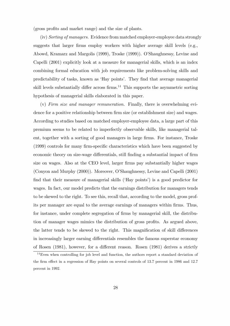
(iv) Sorting of managers. Evidence frommatched employer-employee data strongly

suggests that larger Þrms employ workers with higher average skill levels (e.g.,

Abowd, Kramarz and Margolis (1999), Troske (1999)). O�Shaughnessy, Levine and

Capelli (2001) explicitly look at a measure for managerial skills, which is an index

combining formal education with job requirements like problem-solving skills and

predictability of tasks, known as �Hay points�. They Þnd that average managerial

skill levels substantially differ across Þrms.14 This supports the asymmetric sorting

hypothesis of managerial skills elaborated in this paper.

(v) Firm size and manager remuneration. Finally, there is overwhelming evi-

dence for a positive relationship between Þrm size (or establishment size) and wages.

According to studies based on matched employer-employee data, a large part of this

premium seems to be related to imperfectly observable skills, like managerial tal-

ent, together with a sorting of good managers in large Þrms. For instance, Troske

(1999) controls for many Þrm-speciÞc characteristics which have been suggested by

economic theory on size-wage differentials, still Þnding a substantial impact of Þrm

size on wages. Also at the CEO level, larger Þrms pay substantially higher wages

(Conyon and Murphy (2000)). Moreover, O�Shaughnessy, Levine and Capelli (2001)

Þnd that their measure of managerial skills (�Hay points�) is a good predictor for

wages. In fact, our model predicts that the earnings distribution for managers tends

to be skewed to the right. To see this, recall that, according to the model, gross prof-

its per manager are equal to the average earnings of managers within Þrms. Thus,

for instance, under complete segregation of Þrms by managerial skill, the distribu-

tion of manager wages mimics the distribution of gross proÞts. As argued above,

the latter tends to be skewed to the right. This magniÞcation of skill differences

in increasingly larger earning differentials resembles the famous superstar economy

of Rosen (1981), however, for a different reason. Rosen (1981) derives a strictly14Even when controlling for job level and function, the authors report a standard deviation of

the Þrm effect in a regression of Hay points on several controls of 13.7 percent in 1986 and 12.7

percent in 1992.

28

convex mapping from individual ability to individual earnings from the ability of

more talented individuals (acting as atomistic Þrms) to cover a wider range of mar-

kets. In Rosen (1982), a similar magniÞcation effect arises with respect to manager

remuneration due to a complementarity between supervisory skills and the span of

control. In contrast, in the present analysis, managers develop intangible assets;

and differences in the Þrms� quality of intangible assets tend to become magniÞed

in proÞt differences. In turn, these proÞt differences determine earnings differences

of managers.

6 Conclusion

This paper has focussed on the interaction between product market characteris-

tics and the market for managerial skills. Intangible assets like the organizational

structure of a Þrm, Þrm-speciÞc knowledge, product design, trademarks, etc., play

a key role for the performance of Þrms. Development of intangible assets is the

responsibility of management. Consequently, and according to the main hypothesis

of this paper, managerial quality is a crucial factor for the productivity of Þrms and

the perceived quality of products. It has been argued that, under free entry of ex

ante identical Þrms and geographical non-rivalry of intangible assets, the nature of

product market competition determines how heterogeneous managerial skills sort

into head departments. In turn, this sorting process determines the goods market

structure at single locations and the size distribution of Þrms in the economy.

Standard imperfect competition models imply that given differences among Þrms

in productivity or product quality transmit into increasingly larger differences in

proÞts. This property is related to a high intensity of product market competition.

It has been shown that, under this condition, Þrms tend to differ endogenously in two

dimensions of Þrm size: gross proÞts (typically related to a Þrms� output, sales or

employment level) and the number of plants (market ranges). Thus, paradoxically,

if symmetry breaks down due to an increase in the intensity of product market

competition, �global players� with high market power may emerge in the Þrst place.

29

In particular, the main results of this paper are consistent with the well-known

regularity that the size distribution of Þrms and establishments within industries is

skewed to the right. Moreover, the model predicts that Þrm size is positively re-

lated to productivity, proÞtability, average managerial skills and average managerial

wages. Thus, the model is not only capable to explain why Þrms differ in general,

but provides a uniÞed framework which is consistent with speciÞc observations about

market structures, sorting of managers in Þrms and managerial remuneration.

Appendix

A. Proofs

Proof of Proposition 1. Part (i) is proven Þrst. If 0 < �qi < 1, such that condition

(4) is binding and Q00(�qi) > 0 must hold, we have

∂�qi∂αi

=∂π(αi| �z)/∂αi

Q00(�qi)> 0, (A.1)

according to ∂π(αi|·)∂αi

> 0 from part (i) of Assumption 1 and the implicit function

theorem. To prove part (ii), note that, whenever 0 < �qi < 1,

∂Π(αi| �z)∂αi

=∂�qi∂αi

[π(αi| �z)−Q0(�qi)] + �qi∂π(αi| �z)∂αi

(A.2)

is strictly positive, according to ∂π(αi|·)∂αi

> 0, condition (4) and ∂�qi∂αi

> 0 from part (i).

If �qi = 1, then part (ii) directly follows from∂π(αi|·)∂αi

> 0. This concludes the proof.

¤

Proof of Lemma 1. First, note that

∂2Π(αi| �z)∂α2i

=∂�qi∂αi

∂π(αi| �z)∂αi

+ �qi∂2π(αi| �z)∂α2i

+ (A.3)

∂2�qi∂α2i

[π(αi| �z)−Q0(�qi)] + ∂�qi∂αi

·∂π(αi| �z)∂αi

−Q00(�qi) ∂�qi∂αi

¸,

according to (A.2). If �qi < 1, then∂�qi∂αi> 0 and both terms in square brackets vanish,

according to (4) and (A.1), respectively. If �qi = 1, the latter two summands in (A.3)

also vanish. Thus, ∂�qi∂αi

≥ 0 (from part (ii) of Proposition 1) implies that ∂2Π(αi|�z)∂α2i

> 0

30

if π(αi| �z) is strictly convex in αi. Second, recall that �qi < 1 implies that Q00(�qi) > 0must hold and use (A.1) to obtain

∂2�qi∂α2i

=1

Q00(�qi)2

Ã∂2π(αi| �z)∂α2i

Q00(�qi)−µ∂π(αi| �z)∂αi

¶2Q000(�qi)Q00(�qi)

!. (A.4)

Thus, ∂2�qi∂α2i

> 0 if �qi < 1,∂2π(αi|�z)∂α2i

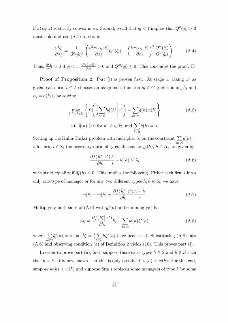
> 0 and Q000(�qi) ≤ 0. This concludes the proof. ¤

Proof of Proposition 2: Part (i) is proven Þrst. At stage 1, taking z∗ as

given, each Þrm i ∈ I chooses an assignment function �gi ∈ �G (determining h̄i and

αi = a(h̄i)) by solving

max�g(h), h∈H

(f

Ã1

s

Xh∈Hh�g(h)

¯̄̄̄¯ z∗!−Xh∈H

�g(h)w(h)

)(A.5)

s.t. �g(h) ≥ 0 for all h ∈ H, andXh∈H

�g(h) = s.

Setting up the Kuhn-Tucker problem with multiplier λi on the constraintPh∈H

�g(h) =

s for Þrm i ∈ I, the necessary optimality conditions for �gi(h), h ∈ H, are given by

∂f( h̄∗i¯̄z∗)

∂h̄i

h

s− w(h) ≤ λi (A.6)

with strict equality if �g∗i (h) > 0. This implies the following. Either each Þrm i hires

only one type of manager or for any two different types h, �h ∈ Si, we have

w(h)− w(�h) = ∂f( h̄∗i¯̄z∗)

∂h̄i

h− �hs. (A.7)

Multiplying both sides of (A.6) with �g∗i (h) and summing yields

sλi =∂f( h̄∗i

¯̄z∗)

∂h̄ih̄i −

Xh∈Hw(h)�g∗i (h), (A.8)

wherePh∈H

�g∗i (h) = s and h̄∗i =

1s

Ph∈Hh�g∗i (h) have been used. Substituting (A.8) into

(A.6) and observing condition (a) of DeÞnition 2 yields (10). This proves part (i).

In order to prove part (ii), Þrst, suppose there exist types h ∈ S and �h /∈ S suchthat h < �h. It is now shown that this is only possible if w(h) < w(�h). For this end,

suppose w(h) ≥ w(�h) and suppose Þrm i replaces some managers of type h by some

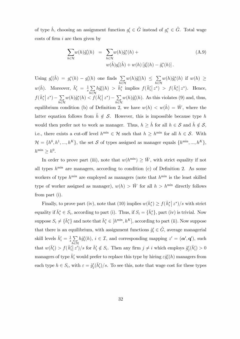
31

of type �h, choosing an assignment function g0i ∈ �G instead of g∗i ∈ �G. Total wage

costs of Þrm i are then given byXh∈Hw(h)�g0i(h) =

Xh∈Hw(h)�g∗i (h) + (A.9)

w(�h)g0i(�h) + w(h) [�g0i(h)− �g∗i (h)] .

Using g0i(�h) = g∗i (h) − g0i(h) one ÞndsPh∈Hw(h)�g0i(h) ≤

Ph∈Hw(h)�g∗i (h) if w(h) ≥

w(�h). Moreover, h̄0i =1s

Ph∈Hh�g0i(h) > h̄∗i implies f( h̄

0i

¯̄z∗) > f( h̄∗i

¯̄z∗). Hence,

f( h̄∗i¯̄z∗)− P

h∈Hw(h)�g∗i (h) < f( h̄

0i

¯̄z∗)− P

h∈Hw(h)�g0i(h). As this violates (9) and, thus,

equilibrium condition (b) of DeÞnition 2, we have w(h) < w(�h) = W̄ , where the

latter equation follows from �h /∈ S. However, this is impossible because type hwould then prefer not to work as manager. Thus, h ≥ �h for all h ∈ S and �h /∈ S,i.e., there exists a cut-off level hmin ∈ H such that h ≥ hmin for all h ∈ S. WithH = {h0, h1, ..., hK}, the set S of types assigned as manager equals {hmin, ..., hK},hmin ≥ h0.In order to prove part (iii), note that w(hmin) ≥ W̄ , with strict equality if not

all types hmin are managers, according to condition (c) of DeÞnition 2. As some

workers of type hmin are employed as managers (note that hmin is the least skilled

type of worker assigned as manager), w(h) > W̄ for all h > hmin directly follows

from part (i).

Finally, to prove part (iv), note that (10) implies w(h̄∗i ) ≥ f( h̄∗i¯̄z∗)/s with strict

equality if h̄∗i ∈ Si, according to part (i). Thus, if Si = {h̄∗i }, part (iv) is trivial. Nowsuppose Si 6= {h̄∗i} and note that h̄∗i ∈ [hmin, hK ], according to part (ii). Now supposethat there is an equilibrium, with assignment functions �g0i ∈ �G, average managerial

skill levels h̄0i =1s

Ph∈Hh�g0i(h), i ∈ I, and corresponding mapping z0 = (α0,q0), such

that w(h̄0i) > f( h̄0i

¯̄z0)/s for h̄0i /∈ Si. Then any Þrm j 6= i which employs �g0j(h̄0i) > 0

managers of type h̄0i would prefer to replace this type by hiring ε�g0i(h) managers from

each type h ∈ Si, with ε = �g0j(h̄0i)/s. To see this, note that wage cost for these types

32

read Xh∈Si

w(h)ε�g0i(h) =�g0j(h̄

0i)

s

Xh∈Si

w(h)�g0i(h) (A.10)

=�g0j(h̄

0i)

sf( h̄0i

¯̄z0),

according to (7). Also note that wage cost w(h̄0i)�gj(h̄0i) are saved. Thus, net wage

cost savings from such a replacement are given by£w(h̄0i)− f( h̄0i

¯̄z0)/s

¤�g0j(h̄

0i), which

is strictly positive if w(h̄0i) > f( h̄0i

¯̄z0)/s for h̄0i /∈ Si, i.e., there would be a proÞtable

deviation. However, according to condition (b) of DeÞnition 2, this is inconsistent

with an equilibrium. Hence, w(h̄∗i ) = f( h̄∗i

¯̄z∗)/s. This concludes the proof. ¤

Proof of Proposition 3. Consider strict convexity of f( h̄i¯̄z∗) in h̄i for all i (at

equilibrium levels) Þrst. Suppose Si 6= {h̄∗i } for some i, i.e., there exist h, �h ∈ Si suchthat �h > h. If Þrm i replaces some managers of type h by some of type �h (i.e., Þrm i

chooses an assignment function �g0i ∈ �G instead of �g∗i ∈ �G) its average managerial skill

rises from h̄∗i to h̄0i > h̄

∗i . (Note that such a replacement is possible since h, �h ∈ Si

implies �g∗i (�h) <Ph∈Si

�g∗i (h) = s and s ≤ g(h) for all h ∈ H by assumption; thus,

�g∗i (�h) < g(�h).) Given z∗, total wage costs for managerial workers in Þrm i then readX

h∈Siw(h)�g0i(h) =

Xh∈Si

w(h)�g∗i (h) + (A.11)

w(h) [�g0i(h)− �g∗i (h)] + w(�h)h�g0i(�h)− �g∗i (�h)

i= f( h̄∗i

¯̄z∗) +

∂f( h̄∗i¯̄z∗)

∂h̄i

h− �hs

[�g0i(h)− �g∗i (h)] ,

where

�g0i(h)− �g∗i (h) = −h�g0i(�h)− �g∗i (�h)

i, (A.12)

(7) and (A.7) have been used. Using h̄0i =1s

Ph∈Si

h�g0i(h) and h̄∗i =

1s

Ph∈Si

h�g∗i (h) together

with (A.12) implies h̄0i − h̄∗i = h−�hs[�g0i(h)− �g∗i (h)]. Hence,X

h∈Siw(h)�g0i(h) = f( h̄i

¯̄z∗) +

∂f( h̄i¯̄z∗)

∂h̄i(h̄0i − h̄∗i ), (A.13)

33

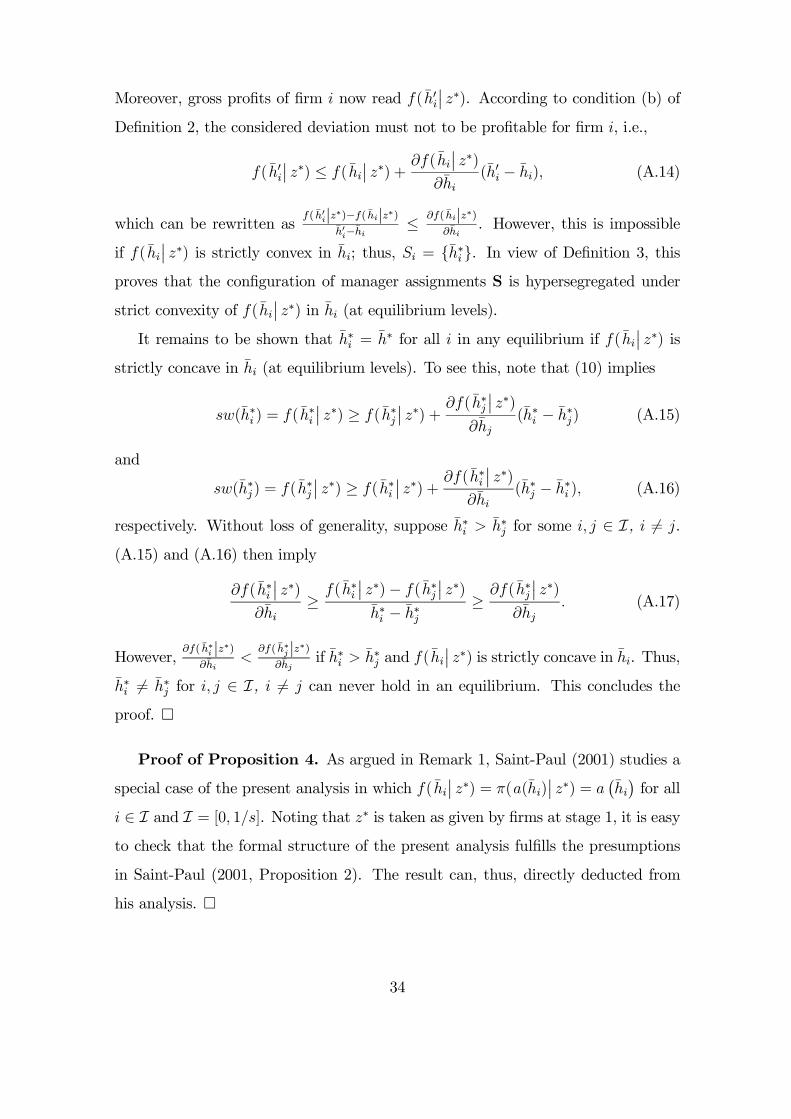
Moreover, gross proÞts of Þrm i now read f( h̄0i¯̄z∗). According to condition (b) of

DeÞnition 2, the considered deviation must not to be proÞtable for Þrm i, i.e.,

f( h̄0i¯̄z∗) ≤ f( h̄i

¯̄z∗) +

∂f( h̄i¯̄z∗)

∂h̄i(h̄0i − h̄i), (A.14)

which can be rewritten asf( h̄0i|z∗)−f( h̄i|z∗)

h̄0i−h̄i≤ ∂f( h̄i|z∗)

∂h̄i. However, this is impossible

if f( h̄i¯̄z∗) is strictly convex in h̄i; thus, Si = {h̄∗i}. In view of DeÞnition 3, this

proves that the conÞguration of manager assignments S is hypersegregated under

strict convexity of f( h̄i¯̄z∗) in h̄i (at equilibrium levels).

It remains to be shown that h̄∗i = h̄∗ for all i in any equilibrium if f( h̄i

¯̄z∗) is

strictly concave in h̄i (at equilibrium levels). To see this, note that (10) implies

sw(h̄∗i ) = f( h̄∗i

¯̄z∗) ≥ f( h̄∗j

¯̄z∗) +

∂f( h̄∗j¯̄z∗)

∂h̄j(h̄∗i − h̄∗j) (A.15)

and

sw(h̄∗j) = f( h̄∗j

¯̄z∗) ≥ f( h̄∗i

¯̄z∗) +

∂f( h̄∗i¯̄z∗)

∂h̄i(h̄∗j − h̄∗i ), (A.16)

respectively. Without loss of generality, suppose h̄∗i > h̄∗j for some i, j ∈ I, i 6= j.

(A.15) and (A.16) then imply

∂f( h̄∗i¯̄z∗)

∂h̄i≥ f( h̄∗i

¯̄z∗)− f( h̄∗j

¯̄z∗)

h̄∗i − h̄∗j≥ ∂f( h̄∗j

¯̄z∗)

∂h̄j. (A.17)

However,∂f( h̄∗i |z∗)

∂h̄i<

∂f( h̄∗j |z∗)∂h̄j

if h̄∗i > h̄∗j and f( h̄i

¯̄z∗) is strictly concave in h̄i. Thus,

h̄∗i 6= h̄∗j for i, j ∈ I, i 6= j can never hold in an equilibrium. This concludes the

proof. ¤

Proof of Proposition 4. As argued in Remark 1, Saint-Paul (2001) studies a

special case of the present analysis in which f( h̄i¯̄z∗) = π(a(h̄i)

¯̄z∗) = a

¡h̄i¢for all

i ∈ I and I = [0, 1/s]. Noting that z∗ is taken as given by Þrms at stage 1, it is easyto check that the formal structure of the present analysis fulÞlls the presumptions

in Saint-Paul (2001, Proposition 2). The result can, thus, directly deducted from

his analysis. ¤

34

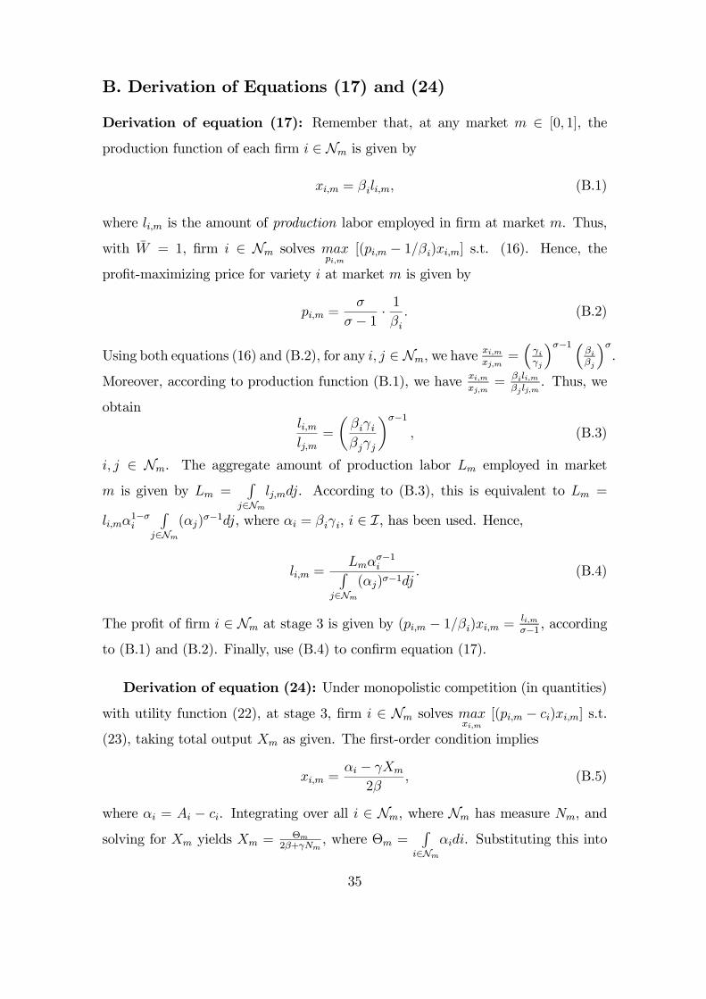
B. Derivation of Equations (17) and (24)

Derivation of equation (17): Remember that, at any market m ∈ [0, 1], the

production function of each Þrm i ∈ Nm is given by

xi,m = βili,m, (B.1)

where li,m is the amount of production labor employed in Þrm at market m. Thus,

with W̄ = 1, Þrm i ∈ Nm solves maxpi,m

[(pi,m − 1/βi)xi,m] s.t. (16). Hence, theproÞt-maximizing price for variety i at market m is given by

pi,m =σ

σ − 1 ·1

βi. (B.2)

Using both equations (16) and (B.2), for any i, j ∈ Nm, we have xi,mxj,m=³γiγj

´σ−1 ³βiβj

´σ.

Moreover, according to production function (B.1), we have xi,mxj,m

=βili,mβj lj,m

. Thus, we

obtainli,mlj,m

=

µβiγiβjγj

¶σ−1, (B.3)

i, j ∈ Nm. The aggregate amount of production labor Lm employed in market

m is given by Lm =R

j∈Nmlj,mdj. According to (B.3), this is equivalent to Lm =

li,mα1−σi

Rj∈Nm

(αj)σ−1dj, where αi = βiγi, i ∈ I, has been used. Hence,

li,m =Lmα

σ−1iR

j∈Nm(αj)σ−1dj

. (B.4)

The proÞt of Þrm i ∈ Nm at stage 3 is given by (pi,m − 1/βi)xi,m = li,mσ−1 , according

to (B.1) and (B.2). Finally, use (B.4) to conÞrm equation (17).

Derivation of equation (24): Under monopolistic competition (in quantities)

with utility function (22), at stage 3, Þrm i ∈ Nm solves maxxi,m

[(pi,m − ci)xi,m] s.t.(23), taking total output Xm as given. The Þrst-order condition implies

xi,m =αi − γXm

2β, (B.5)

where αi = Ai − ci. Integrating over all i ∈ Nm, where Nm has measure Nm, and

solving for Xm yields Xm = Θm2β+γNm

, where Θm =R

i∈Nmαidi. Substituting this into

35

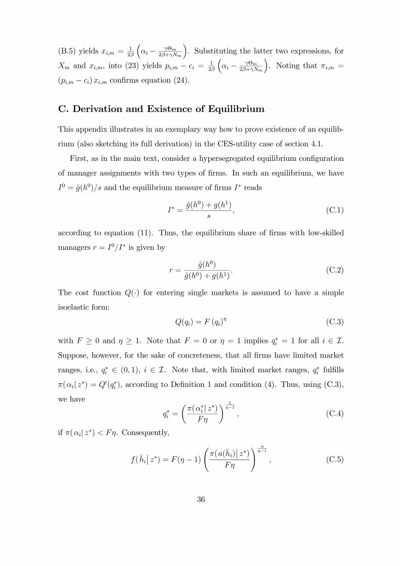
(B.5) yields xi,m = 12β

³αi − γΘm

2β+γNm

´. Substituting the latter two expressions, for

Xm and xi,m, into (23) yields pi,m − ci = 12β

³αi − γΘm

2β+γNm

´. Noting that πi,m =

(pi,m − ci) xi,m conÞrms equation (24).

C. Derivation and Existence of Equilibrium

This appendix illustrates in an exemplary way how to prove existence of an equilib-

rium (also sketching its full derivation) in the CES-utility case of section 4.1.

First, as in the main text, consider a hypersegregated equilibrium conÞguration

of manager assignments with two types of Þrms. In such an equilibrium, we have

I0 = �g(h0)/s and the equilibrium measure of Þrms I∗ reads

I∗ =�g(h0) + g(h1)

s, (C.1)

according to equation (11). Thus, the equilibrium share of Þrms with low-skilled

managers r = I0/I∗ is given by

r =�g(h0)

�g(h0) + g(h1). (C.2)

The cost function Q(·) for entering single markets is assumed to have a simpleisoelastic form:

Q(qi) = F (qi)η (C.3)

with F ≥ 0 and η ≥ 1. Note that F = 0 or η = 1 implies q∗i = 1 for all i ∈ I.Suppose, however, for the sake of concreteness, that all Þrms have limited market

ranges, i.e., q∗i ∈ (0, 1), i ∈ I. Note that, with limited market ranges, q∗i fulÞllsπ(αi| z∗) = Q0(q∗i ), according to DeÞnition 1 and condition (4). Thus, using (C.3),we have

q∗i =µπ(α∗i | z∗)Fη

¶ 1η−1, (C.4)

if π(αi| z∗) < Fη. Consequently,

f( h̄i¯̄z∗) = F (η − 1)

Ãπ(a(h̄i)

¯̄z∗)

Fη

! ηη−1

, (C.5)

36

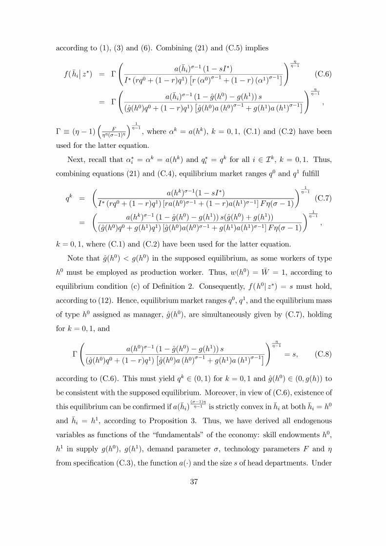
according to (1), (3) and (6). Combining (21) and (C.5) implies

f( h̄i¯̄z∗) = Γ

Ãa(h̄i)

σ−1 (1− sI∗)I∗ (rq0 + (1− r)q1) £r (α0)σ−1 + (1− r) (α1)σ−1¤

! ηη−1

(C.6)

= Γ

Ãa(h̄i)

σ−1 (1− �g(h0)− g(h1)) s(�g(h0)q0 + (1− r)q1) £�g(h0)a (h0)σ−1 + g(h1)a (h1)σ−1¤

! ηη−1

,

Γ ≡ (η − 1)³

Fηη(σ−1)η

´ 1η−1, where αk = a(hk), k = 0, 1, (C.1) and (C.2) have been

used for the latter equation.

Next, recall that α∗i = αk = a(hk) and q∗i = qk for all i ∈ Ik, k = 0, 1. Thus,

combining equations (21) and (C.4), equilibrium market ranges q0 and q1 fulÞll

qk =

µa(hk)σ−1(1− sI∗)

I∗ (rq0 + (1− r)q1) [ra(h0)σ−1 + (1− r)a(h1)σ−1]Fη(σ − 1)¶ 1

η−1(C.7)

=

µa(hk)σ−1 (1− �g(h0)− g(h1)) s(�g(h0) + g(h1))

(�g(h0)q0 + g(h1)q1) [�g(h0)a(h0)σ−1 + g(h1)a(h1)σ−1]Fη(σ − 1)¶ 1

η−1,

k = 0, 1, where (C.1) and (C.2) have been used for the latter equation.

Note that �g(h0) < g(h0) in the supposed equilibrium, as some workers of type

h0 must be employed as production worker. Thus, w(h0) = W̄ = 1, according to

equilibrium condition (c) of DeÞnition 2. Consequently, f(h0| z∗) = s must hold,

according to (12). Hence, equilibriummarket ranges q0, q1, and the equilibriummass

of type h0 assigned as manager, �g(h0), are simultaneously given by (C.7), holding

for k = 0, 1, and

Γ

Ãa(h0)σ−1 (1− �g(h0)− g(h1)) s

(�g(h0)q0 + (1− r)q1) £�g(h0)a (h0)σ−1 + g(h1)a (h1)σ−1¤! η

η−1

= s, (C.8)

according to (C.6). This must yield qk ∈ (0, 1) for k = 0, 1 and �g(h0) ∈ (0, g(h)) tobe consistent with the supposed equilibrium. Moreover, in view of (C.6), existence of

this equilibrium can be conÞrmed if a(h̄i)(σ−1)ηη−1 is strictly convex in h̄i at both h̄i = h0

and h̄i = h1, according to Proposition 3. Thus, we have derived all endogenous

variables as functions of the �fundamentals� of the economy: skill endowments h0,

h1 in supply g(h0), g(h1), demand parameter σ, technology parameters F and η

from speciÞcation (C.3), the function a(·) and the size s of head departments. Under

37

appropriate assumptions about these fundamentals, the supposed equilibrium exists.

According to Proposition 1, f(h1| z∗) > f(h0| z∗) and q1 > q0 for gross proÞts andmarket ranges, respectively. Wages read w(h1) = f(h1| z∗)/s > f(h0| z∗)/s =w(h0) = W̄ = 1 in this example, according to Proposition 2.

Second, analogously, suppose the conÞguration of manager assignment is sym-

metric, i.e., h̄∗i = h̄∗ and, thus, α∗i = a(h̄

∗) and q∗i = q∗ for all i ∈ I. For simplicity,

let Q(·) ≡ 0 such that q∗ = 1. Hence, Ξm = Ξ∗ = I∗a(h̄∗)σ−1 for all m. Again, letthere be two skill types h0 and h1, h0 < h1, both types being assigned as manager.

Using this together with q∗ = 1, Q(1) = 0 and L∗ = 1− �g(h0)− g(h1) (labor marketclearing), one obtains

f( h̄i¯̄z∗) =

a(h̄i)σ−1(1− �g(h0)− g(h1))

(�g(h0) + g(h1)) a(h̄∗)σ−1s

σ − 1 , (C.9)

according to (3), (6), (17) and (C.1). Thus, we have

f( h̄∗¯̄z∗) =

1− �g(h0)− g(h1)�g(h0) + g(h1)

s

σ − 1 (C.10)

and∂f( h̄∗

¯̄z∗)

∂h̄i=1− �g(h0)− g(h1)�g(h0) + g(h1)

a0(h̄∗)sa(h̄∗)

, (C.11)

respectively, where h̄∗ = h0�g(h0)+h1g(h1)�g(h0)+g(h1)

, according to equation (13). Using equations

(14), (C.10) and (C.11), as well as h0 = hmin and w(h0) = W̄ = 1, �g(h0) is given by

1− �g(h0)− g(h1)�g(h0) + g(h1)

µ1

σ − 1 +a0(h̄∗)a(h̄∗)

(h0 − h̄∗)¶= 1. (C.12)

A symmetric equilibrium exists if this yields �g(h0) ∈ (0, g(h)) and a(h̄i)σ−1 is strictlyconcave in h̄i at h̄i = h̄∗. Finally,

w(h1) =1− �g(h0)− g(h1)�g(h0) + g(h1)

µ1

σ − 1 +a0(h̄∗)a(h̄∗)

(h1 − h̄∗)¶. (C.13)

References

Abowd, John M., Francis Kramarz and David N. Margolis (1999). High Wage

Workers and High Wage Firms, Econometrica 67 (2), 251-333.

38

Athey, Susan and Armin Schmutzler (2001). Investment and Market Dominance,

RAND Journal of Economics 32 (1), 1-26.

Baily, Martin N., Charles Hulten and David Campbell (1992). The Distribution

of Productivity in Manufacturing Plants, Brookings Papers of Economic Activity 0,

Microeconomics, 187-249.

Bartelsman, Eric J. and Mark Domes (2000). Understanding Productivity:

Lessons from Longitudinal Microdata, Journal of Economic Literature 38 (3), 569-

594.

Berman, Eli, John Bound, and Zvi Grichilis (1994). Changes in the Demand

for Skilled Labor Within U.S. Manufacturing: Evidence from the Annual Survey of

Manufactures, Quarterly Journal of Economics 109 (2), 367-397.

Bresnahan, Timothy F. (1999). Computerisation and Wage Dispersion: An

Analytical Reinterpretation, Economic Journal 109, F390-F415.

Caves, Richard E. (1982). Multinational Enterprise and Economic Analysis

(London: Cambridge University Press).

Coase, Ronald (1937). The Nature of the Firm, Economica 4, 386-405.

Conyon, Martin J. and Kevin M. Murphy (2000). The Prince and the Pauper?

CEO Pay in the United States and United Kingdom, Economic Journal 110, F640-

F671.

Dixit, Avinash and Joseph E. Stiglitz (1977). Monopolistic Competition and

Optimum Product Diversity, American Economic Review 67, 297-308.

Dunning, John H. (1981). International Production and the Multinational En-

terprise (London: Allen and Unwin).

Fishman, Arthur and Rafael Rob (1999). The Size of Firms and R&D Invest-

ment, International Economic Review 40 (4), 915-931.

Grossman, Sanford and Oliver Hart (1986). The Costs and BeneÞts of Owner-

ship: A Theory of Lateral and Vertical Integration, Journal of Political Economy

94, 691-719.

Grossmann, Volker (2002). Quality Improvements, the Structure of Employ-

ment, and the Skill-Bias Hypothesis Revisited, Topics in Macroeconomics 2 (1),

39

Article 2, http://www.bepress.com/bejm/topics/vol2/iss1/art2/.

Hart, Oliver and John Moore (1990). Property Rights and the Nature of the

Firm, Journal of Political Economy 98, 1119-1158.

Helpman, Elhanan (1981). International Trade in the Presence of Product Dif-

ferentiation, Economies of Scale and Monopolistic Competition, Journal of Interna-

tional Economics 11, 305-40.

Holmström, Bengt and Paul Milgrom (1991). Multitask Principal-Agent Analy-

ses: Incentive Contracts, Asset Ownership, and Job Design, Journal of Law, Eco-

nomics, and Organization 7, 24-51.

Holmström, Bengt and Paul Milgrom (1994). The Firm as an Incentive System,

American Economic Review 84, 972-991.

Holmström, Bengt and John Roberts (1998). The Boundaries of the Firm Re-

visited, Journal of Economic Perspectives 12 (4), 73-94.

Hotelling, Harold (1929). Stability in Competition, Economic Journal 39, 41-57.

Jovanovic, Boyan (1982). Selection and the Evolution of Industry, Econometrica

50, 649-670.

Kremer, Michael (1993). The O-Ring Theory of Economic Development, Quar-

terly Journal of Economics 108 (3), 551-75.

Kremer, Michael and Erik Maskin (1996). Wage Inequality and Segregation by

Skill, NBER Working Paper No. 5718.

Lancaster, Kelvin (1979). Variety, Equity, and Efficiency, Columbia University

Press.

Lucas, Robert, E. (1978). On the Size Distribution of Business Firms, Bell

Journal of Economics 9 (2), 508-523.

Markusen, James R. (1995). The Boundaries of Multinational Enterprises and

the Theory of International Trade, Journal of Economic Perspectives 9 (2), 169-189.

Martin, Stephen (1991). Direct Foreign Investment, Journal of Economic Be-

havior and Organization 16, 283-293.

Morck, Randall and Bernard Yeung (1992). Internationalization: An Event

Study Test, Journal of International Economics 33 (1-2), 41-56.

40

Ottaviano, Gianmarco I.P. and Jacques-François Thisse (1999). Monopolistic

Competiton, Multiproduct Firms and Optimum Product Diversity, CORE Discus-

sion Paper No. 9919.

O�Shaughnessy, K.C., David I. Levine and Peter Capelli (2001). Changes in

Managerial Pay Structures 1986-1992 and Rising Returns to Skill, Oxford Economic

Papers 3, 482-507.

Porter, Michael E. (1986). Changing Patterns of International Competition,

California Management Review 28 (2), 9-40.

Prat, Andrea (2002). Should a Team be Homogenous, European Economic Re-

view 46 (7), 1187-1207.

Roberts, Mark J. and Dylan Supina (2000). Output Price and Markup Disper-

sion in Producer Micro Data: The Roles of Producer Heterogeneity and Noise, in:

Baye, M. (Ed.), Advances in Applied Microeconomics, Vol. 9, Industrial Organiza-

tion (JAI Press).

Rosen, Sherwin (1981). The Economics of Superstars, American Economic Re-

view 71 (5), 845-858.

Rosen, Sherwin (1982). Authority, Control, and the Distribution of Earnings,

Bell Journal of Economics 13 (2), 311-323.

Saint-Paul, Gilles (2001). On the Distribution of Income andWorker Assignment

Under IntraÞrm Spillovers, with an Application to Ideas and Networks, Journal of

Political Economy 109 (1), 1-37.

Salop, Steven C. (1979). Monopolistic Competition with Outside Goods, Bell

Journal of Economics 10 (1), 141-56.

Sattinger, Michael (1993). Assignment Models of the Distribution of Earnings,

Journal of Economic Literature 31 (2), 831-880.

Salamon, Gerald L. (1985). Accounting Rates of Return, American Economic

Review 75, 495-504.

Schmalensee, Richard (1989). Inter-Industry Studies of Structures and Perfor-

mance, in: Schmalensee, R. and R. Willig (Eds.), Handbook of Industrial Organi-

zation, Vol. 2, 951-1009.

41

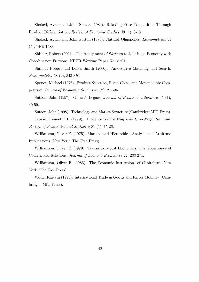
Shaked, Avner and John Sutton (1982). Relaxing Price Competition Through

Product Differentiation, Review of Economic Studies 49 (1), 3-13.

Shaked, Avner and John Sutton (1983). Natural Oligopolies, Econometrica 51

(5), 1469-1483.

Shimer, Robert (2001). The Assignment of Workers to Jobs in an Economy with

Coordination Frictions, NBER Working Paper No. 8501.

Shimer, Robert and Lones Smith (2000). Assortative Matching and Search,

Econometrica 68 (2), 343-370.

Spence, Michael (1976). Product Selection, Fixed Costs, and Monopolistic Com-

petition, Review of Economic Studies 43 (2), 217-35.

Sutton, John (1997). Gibrat�s Legacy, Journal of Economic Literature 35 (1),

40-59.

Sutton, John (1998). Technology andMarket Structure (Cambridge: MIT Press).

Troske, Kenneth R. (1999). Evidence on the Employer Size-Wage Premium,

Review of Economics and Statistics 81 (1), 15-26.

Williamson, Oliver E. (1975). Markets and Hierarchies: Analysis and Antitrust

Implications (New York: The Free Press).

Williamson, Oliver E. (1979). Transaction-Cost Economics: The Governance of

Contractual Relations, Journal of Law and Economics 22, 233-271.

Williamson, Oliver E. (1985). The Economic Institutions of Capitalism (New

York: The Free Press).

Wong, Kar-yiu (1995). International Trade in Goods and Factor Mobility (Cam-

bridge: MIT Press).

42

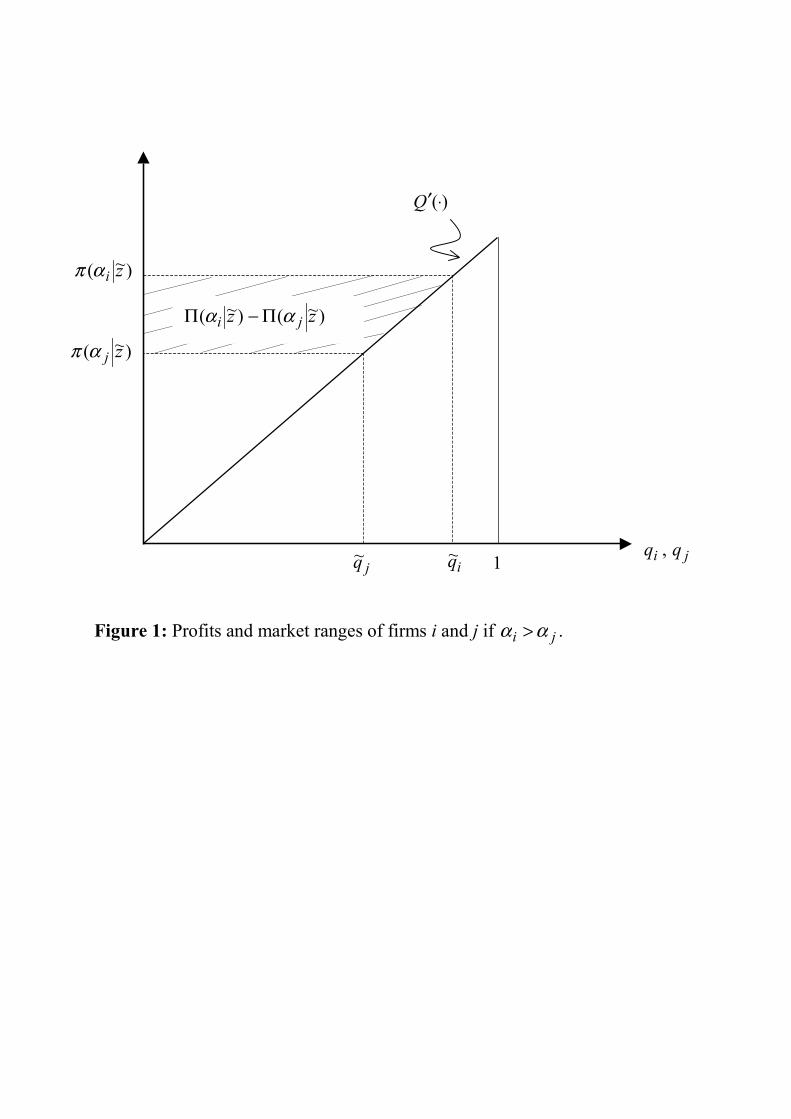
Figure 1: Profits and market ranges of firms i and j if ji αα > .

)(⋅′Q

ji qq ,jq~

)~( ziαπ

1

)~( ziαΠ )~( zjαΠ−

)~( zjαπ

iq~

Figure 2: Convexity and segregation by managerial skill.

h

shh

hhf

shf i

i

ii −⋅

∂⋅∂

+⋅ )()(

ih ih ′h~ h�

shf )( ⋅

A

B

C

D

IZA Discussion Papers No.

Author(s) Title

Area Date

723 M. Coles B. Petrongolo

A Test between Unemployment Theories Using Matching Data

3 02/03

724 J. T. Addison R. Bailey W. S. Siebert

The Impact of Deunionisation on Earnings Dispersion Revisited

2 02/03

725 S. Habermalz An Examination of Sheepskin Effects Over Time 1 02/03

726 S. Habermalz Job Matching and the Returns to Educational Signals

1 02/03

727 M. Raiser M. Schaffer J. Schuchardt

Benchmarking Structural Change in Transition 4 02/03

728 M. Lechner J. A. Smith

What is the Value Added by Caseworkers? 6 02/03

729 A. Voicu H. Buddelmeyer

Children and Women's Participation Dynamics: Transitory and Long-Term Effects

3 02/03

730 M. Piva M. Vivarelli

Innovation and Employment: Evidence from Italian Microdata

2 02/03

731 B. R. Chiswick N. DebBurman

Educational Attainment: Analysis by Immigrant Generation

1 02/03

732 A. Falk A. Ichino

Clean Evidence on Peer Pressure 5 03/03

733 S. Wolter S. Denzler

Wage Elasticity of the Teacher Supply in Switzerland

2 03/03

734 S. Wolter Sibling Rivalry: A Six Country Comparison 2 03/03

735 R. Desmet A. Jousten S. Perelman P. Pestieau

Micro-Simulation of Social Security Reforms in Belgium

3 03/03

736 I. Bolvig P. Jensen M. Rosholm

The Employment Effects of Active Social Policy 6 03/03

737 A. L. Booth M. Francesconi G. Zoega

Unions, Work-Related Training, and Wages: Evidence for British Men

3 03/03

738 V. Grossmann Managerial Job Assignment and Imperfect Competition in Asymmetric Equilibrium

1 03/03

An updated list of IZA Discussion Papers is available on the center‘s homepage www.iza.org.