Management Science - Columbia Universitymnb2/broadie/Assets/bg-ms-1996.pdf · This paper appeared...

This paper appeared in Management Science, 1996, Vol. 42, No. 2, 269–285.

Estimating Security Price Derivatives Using Simulation

Mark Broadie∗

Paul Glasserman∗

October 20, 1993

Revised: July 8, 1994

Abstract

Simulation has proved to be a valuable tool for estimating security prices for which simple

closed form solutions do not exist. In this paper we present two direct methods, a pathwise

method and a likelihood ratio method, for estimating derivatives of security prices using sim-

ulation. With the direct methods, the information from a single simulation can be used to

estimate multiple derivatives along with a security’s price. The main advantage of the direct

methods over re-simulation is increased computational speed. Another advantage is that the

direct methods give unbiased estimates of derivatives, whereas the estimates obtained by re-

simulation are biased. Computational results are given for both direct methods and compar-

isons are made to the standard method of re-simulation to estimate derivatives. The methods

are illustrated for a path independent model (European options), a path dependent model

(Asian options), and a model with multiple state variables (options with stochastic volatility).

Keywords: Simulation, derivative estimation, security pricing, option pricing.

∗Both authors are at the Graduate School of Business, Columbia University, New York, NY,

10027, USA.

1. Introduction

In this paper two direct methods for estimating security price derivatives using Monte

Carlo simulation are presented, a pathwise method and a likelihood ratio method. The stan-

dard indirect method of estimating a security price derivative is re-simulation. In this ap-

proach, an initial simulation is run to determine a base price, then the parameter of interest

is perturbed and another simulation is run to determine a perturbed price. The estimate of

the derivative is the difference in the simulated prices divided by the parameter perturbation.

The direct methods proposed in this paper offer increased computational speed, in that they

avoid the need to run additional simulations. The output from the initial simulation contains

considerable information that can be used to estimate security price derivatives directly. This

advantage becomes more pronounced as the number of derivatives to be estimated increases.

While the re-simulation approach requires one additional simulation run for each derivative

to be estimated, the direct methods require information only from the initial simulation run.

A second advantage of the direct methods is that they give unbiased estimates of derivatives,

whereas the re-simulation estimates are generally biased.

Boyle (1977) proposed the use of Monte Carlo simulation for estimating security prices.

Since that time, simulation has proved to be a valuable tool in many situations where other

tools are not available or are not practical to implement. For example, simulation is useful

for estimating security prices when there is no analytical expression for the terminal distri-

bution of the security price, when there are multiple state variables, and when there are path

dependent payoffs. Simulation has been used to estimate prices of contingent claims, prices

of mortgage backed securities, and to value swaps. Simulation is generally not appropriate for

valuing American-style contingent claims, i.e., securities with opportunities for optimal early

exercise. A complete survey of successful applications of the simulation approach would be

too extensive to include here. However, for a brief sampling of the literature the reader is

referred to Boyle (1977), Hull and White (1987), Johnson and Shanno (1987), Jones and Ja-

cobs (1986), Kemna and Vorst (1990), Schwartz and Torous (1989), and Smith, Smithson, and

Wilford (1990).

The focus of this paper is using simulation to estimate security price derivatives. Deriva-

tive information is of practical and theoretical importance. For practitioners, derivative in-

formation is important for hedging, i.e., for reducing the risk of a security or portfolio of

securities, when closing the position is not practical or desirable. For example, the derivative

of an option price with respect to the price of the underlying security (i.e., the delta) indicates

the number of units of the security to hold in the hedge portfolio. The corresponding second

Estimating Security Price Derivatives Using Simulation 2

derivative (i.e., the gamma) is related to the optimal time interval required for rebalancing a

hedge under transactions costs. Other derivative information is useful for protecting against

changes in the associated parameters, e.g., changes in volatility, time to maturity, or interest

rates. On the theoretical side, Breeden and Litzenberger (1978) show that the second deriva-

tive with respect to the strike price can be interpreted as a state price density. Carr (1993)

shows how first and higher order derivatives of an option’s price with respect to the initial

price of the underlying security can be viewed as an expectation, under an appropriate change

of measure, of the corresponding derivative at the terminal date.

To estimate derivatives via simulation, two direct methods are investigated. The pathwise

method is based on the relationship between the security payoff and the parameter of interest.

Differentiating this relationship leads, under appropriate conditions, to an unbiased estimator

for the derivative of the security price. In contrast, the likelihood ratio method, is based on

the relationship between the probability density of the price of the underlying security and

the parameter of interest. These methods have been studied in the discrete-event simulation

literature, but have not received much attention in financial applications. Fu and Hu (1993b)

also derive pathwise derivative estimates in the case of a European call option on a single

underlying asset and illustrate their use in optimization. For an overview of the pathwise

method, see Glasserman (1991), and for the likelihood ratio method (also called the score

function method) see Glynn (1987) and Rubinstein and Shapiro (1993).

The direct methods are described in detail through an example in Section 2. For ease of

exposition, the example chosen in Section 2 is a European option on a dividend paying asset,

an example for which simulation is not required. While both direct methods lead to unbiased

estimators, they differ in their effectiveness and scope of applicability. Second derivative es-

timators are developed in Section 3. Computational comparisons of the two direct methods

and the indirect re-simulation method are given in Section 4. To illustrate a range of applica-

tions, the examples in Section 4 include Asian options (path dependent payoffs) and options

in a stochastic volatility setting (multiple state variables). Concluding remarks are given in

Section 5. Detailed formulas and technical results are given in the appendices.

2. Derivative Estimates for European Call Options

In this section, the pathwise and likelihood ratio methods are developed for estimating

sensitivities of security prices through simulation. For expository purposes, the two methods

are introduced through a simple example — one for which simulation is not required. Consider

the price p of a European call option on a dividend paying asset that follows a lognormal

diffusion. In particular, assume that the risk neutralized price of the underlying asset, St ,


satisfies the stochastic differential equation

dSt = St[(r − δ)dt + σ dBt], (1)

where Bt is a standard Brownian motion process (see Hull (1992) for a general discussion of

this model). In equation (1), r is the riskless interest rate, δ is the dividend rate, and σ > 0

is the volatility parameter. Under the risk neutral measure, ln(ST /S0) is normally distributed

with mean (r −δ−σ 2/2)T and variance σ 2T . The option has a strike price of K and matures

at time T > 0, with the current time taken to be t = 0. In this “Black-Scholes world”, the option

price is given by

p = E[e−rT max(ST −K,0)]. (2)

Throughout the paper, E denotes the expectation operator under the risk neutral measure.

See Harrison and Kreps (1979) for a justification of this pricing formula.

Pathwise Derivatives

To illustrate the application of the first method, we consider the problem of estimating

vega, which is dp/dσ . We do this by defining the discounted payoff

P = e−rT max(ST −K,0), (3)

(so that p = E[P]) and examining how changes in σ determine changes in P . Since σ affects

P only through ST , we begin by examining the dependence of ST on σ .

The lognormal random variable ST can be represented as

ST = S0e(r−δ−12σ

2)T+σ√TZ, (4)

where Z is a standard normal random variable. Consequently,

dSTdσ

= ST (−σT +√TZ)

= STσ[ln(ST /S0)− (r − δ+ 1

2σ2)T]. (5)

This tells us how a small change in σ affects ST . Now consider the effect on P of a small change

in ST . If ST ≥ K, then the option is in the money and any increase ∆ in ST translates into an

increase e−rT∆ in P . If, however, ST < K, then P = 0, and P remains 0 for all sufficiently small

changes in ST . Thus, we arrive at the formal expression

dPdST

= e−rT1{ST≥K}, (6)


in which 1{·} denotes the indicator of the event in braces.1 Combining (5) and (6) gives

dPdσ

= dPdST

dSTdσ

= e−rT1{ST≥K}STσ[ln(ST /S0)− (r − δ+ 1

2σ2)T]. (7)

Each of the terms in this expression is easily evaluated in a simulation, making the estimator

dP/dσ easy to use. Moreover, it follows from Proposition 1 in Appendix A that this estimator

is unbiased, i.e.,

E[dPdσ

] = dpdσ

.

A similar argument leads to an estimator of delta, the derivative of the option price with

respect to the initial price of the underlying asset. Much as before, we have

dPdS0

= dPdST

dSTdS0

= e−rT1{ST≥K}dSTdS0

. (8)

Furthermore, from (4) we find that

dSTdS0

= e(r−δ−12σ

2)T+σ√TZ = STS0.

Substituting this into (8), we arrive at the estimator

dPdS0

= e−rT1{ST≥K}STS0. (9)

This estimator is also unbiased, i.e.,

E[ dPdS0

] = dpdS0

.

Similar arguments can be used to develop derivative estimates for options with path dependen-

cies, for which simulation is often the only available computational approach (see Section 4).

Derivatives Based on Likelihood Ratios

The second method of estimating derivatives puts the dependence on the parameter of

interest in an underlying probability density, rather than in a random variable. We continue

with the European option example. It follows from (4) that under the risk neutral measure,

the density of ST is

g(x) = 1

xσ√Tn(d(x)), x ≥ 0, (10)

1 Equation (6) is valid if interpreted as a righthand derivative or as the almost everywhere defined derivativeof a Lipschitz function. Technical issues of this type are treated in Appendix A.


where n(z) = 1√2π e

−z2/2 is the standard normal density and

d(x) = ln(x/S0)− (r − δ− 12σ

2)Tσ√T

. (11)

Thus, we can write (2) as

p =∫∞

0e−rT max(x −K,0)g(x)dx. (12)

We now use this representation of p to derive derivative estimates. We begin by consid-

ering dp/dσ . Notice that in (12), σ appears only as an argument of g. Assuming we can

interchange the derivative and integral, (12) implies that

dpdσ

=∫∞

0e−rT max(x −K,0)∂g(x)

∂σdx. (13)

Multiplying and dividing the integrand in (13) by g(x) and using the identity (∂g/∂σ)/g =∂ lng/∂σ , gives

dpdσ

=∫∞

0e−rT max(x −K,0)∂ ln(g(x))

∂σg(x)dx

= E[e−rT max(ST −K,0)∂ ln(g(ST ))∂σ

].

This indicates that the likelihood ratio estimator

e−rT max(ST −K,0)∂ ln(g(ST ))∂σ

(14)

is an unbiased estimator of dp/dσ when ST is simulated under the risk neutral measure. The

estimator in (14) is easily implemented using the formula

∂ ln(g(x))∂σ

= −d ∂d∂σ

− 1σ, (15)

where d is given in (11) and

∂d∂σ

= ln(S0/x)+ (r − δ+ 12σ

2)Tσ 2√T

.

A similar argument provides an estimator of the derivative with respect to the initial asset

price. Proceeding just as before, we arrive at the equation

dpdS0

= E[e−rT max(ST −K,0)∂ ln(g(ST ))∂S0

],

and hence obtain the unbiased likelihood ratio estimator

e−rT max(ST −K,0)∂ ln(g(ST ))∂S0

, (16)

where∂ ln(g(x))

∂S0= d(x)S0 σ

√T

= ln(x/S0)− (r − δ− 12σ

2)TS0 σ 2T

.

The estimator in (16) is easily used in a simulation of ST .


Discussion

We have seen through the European call option example that it is sometimes possible to

obtain estimates of derivatives of security prices without re-simulation. The same methods

apply when closed form expressions are not available and simulation is necessary. In general,

the estimators obtained through the pathwise method and the likelihood ratio method are not

the same. Numerical comparisons are presented in Section 4. At this point, we make some

general observations about direct methods compared with re-simulation and the scope of the

methods discussed above.

Both pathwise derivative estimates and estimates based on likelihood ratios require an

interchange of a derivative and an integral (expectation) for unbiasedness. It is largely this

requirement that limits their scope, though the limitation is rarely an issue with standard

pricing models. Classical conditions for this interchange require fairly strong smoothness

conditions on the integrand; see, e.g., Franklin (1944), pp. 150–151. These conditions are

typically satisfied by the probability densities arising in applications of the likelihood ratio

method to pricing models. Indeed, the density in (10) is continuously differentiable in each

of its parameters on its domain. In contrast, the pathwise dependence of the payoff of a

derivative security may not be smooth. For example, the expression in (3) is continuous in STbut fails to be differentiable at the point ST = K. As a consequence, somewhat greater care is

required with this method in justifying the interchange of derivative and integral. As a rough

rule of thumb, if the payoff is continuous, the pathwise method is typically applicable; see

Appendix A for a more precise discussion.

Since smoothness is rarely a problem for densities, the main limitation in the application

of the likelihood ratio method is that the parameter of interest may not be a parameter of the

density at all. This is the case with the strike price in (2); the likelihood ratio method does

not apply to this parameter (except possibly through a change of variables). The pathwise

method, however, easily covers this case.

It is important to note that the derivation of the likelihood ratio estimator (14) did not

make use of any properties of the dependence of the option payoff on the underlying asset

price. That is, the particular form of (3) was not important, except for the fact that it displays

no explicit dependence on σ . As a consequence, essentially the same estimator applies to any

derivative security. If the discounted payoff associated with some security is f , meaning that

its price is given by p = E[f(ST )], then its derivative with respect to σ is given by

dpdσ

= E[f(ST )∂ ln(g(ST ))∂σ

],

subject only to the validity of the interchange of derivative and integral. This contrasts


markedly with the pathwise method, which depends in an essential way on the form of the

payoff. Using the pathwise method, one must derive a different estimator for each payoff

function. On one hand, this distinction represents an implementation advantage for the like-

lihood ratio method; on the other hand, it suggests that the pathwise method is better able to

exploit the structure of individual problems.

3. Second Derivatives

The gamma of an option, i.e., the second derivative with respect to the initial price of the

underlying security, is related to the optimal time interval required for rebalancing a hedge

under transactions costs. In this section the direct methods are extended to the estimation of

second derivatives.

Pathwise Second Derivative Estimators

We begin our discussion by considering the simple (if artificial) case of an exponential

payoff. Suppose that the payoff of a contingent claim is e−ST when the final price of the

underlying security is ST . Then the value of this claim today is

p = E[e−rT e−ST ].

Consider the second derivative of p with respect to the initial price S0. Differentiating twice

inside the expectation gives

d2pdS2

0

= E[e−rT e−ST

{(dSTdS0

)2

− d2STdS2

0

}].

From (4), we find that dST/dS0 = ST/S0 and d2ST/dS20 = 0. Making these substitutions, we

getd2pdS2

0

= E[e−rT e−ST

(STS0

)2].

Now let p once again be the European option price in (2). From (9) we have

dp(S0)dS0

= E[e−rT (ST (S0)S0

)1{ST (S0)≥K}], (17)

where the dependence of ST on S0 is made explicit. Consider a small increase h in S0. Since

the ratio ST/S0 does not depend on S0, we get

dp(S0 + h)dS0

− dp(S0)dS0

= E[e−rT (STS0

)(1{ST (S0+h)≥K} − 1{ST (S0)≥K})]

= E[e−rT (STS0

)1{ST (S0+h)≥K>ST (S0)}]

= E[e−rT (STS0

)1{ST (S0)+ dST (S0)

dS0h≥K>ST (S0)}].


Dividing by h and letting h decrease to zero, the expectation becomes concentrated at ST = K.

Using dST (S0)/dS0 = ST/S0, this gives2

d2pdS2

0

= e−rT ( KS0

)2g(K)

= e−δT n(d1(K))S0σ

√T, (18)

where d1(x) = [ln(S0/x)+(r−δ+ 12σ

2)T]/(σ√T) = −d(x)+σ√T .3 Expression (18) involves

no random quantities and thus requires no simulation. Indeed, the result is the well known

formula for the gamma of an option, which is usually derived without reference to simulation

(see, e.g., Hull (1992), p. 312). The effect of the expectation in (17) is to “smooth” the indicator

function. We will see in Section 4 that similar smoothing arguments result in nontrivial second

derivative estimators in settings where no closed form expression exists.

Likelihood Ratio Second Derivative Estimators

Consider again the problem of estimating the second derivative of p in (2) with respect to

the initial asset price S0. Starting from (12) and differentiating twice under the integral gives

d2pdS2

0

=∫∞

0e−rT max(x −K,0)∂

2g(x)∂S2

0

dx.

Multiplying and dividing the integrand by g(x) turns the integral into an expectation and

yieldsd2pdS2

0

= E[e−rT max(ST −K,0)∂2g(ST )∂S2

0

1g(ST )

].

The expression

e−rT max(ST −K,0)∂2g(ST )∂S2

0

1g(ST )

is thus an unbiased likelihood ratio estimator of the second derivative. The estimator can be

written more explicitly using

∂2g(ST )∂S2

0

1g(ST )

= d2 − dσ√T − 1

S20σ 2T

,

where d = d(ST ) is given in (11).

2 The same result can be derived in another way. Taking the derivative of (17) again with respect to S0 gives

d2pdS2

0

= E[e−rT(STS0

) ∂∂S0

1{ST (S0)≥K}] = e−rT( KS0

)2g(K).

The second equality uses d1{ST (S0)≥K}/dS0 = δ(K)dST /dS0 = δ(K)ST /S0, where δ(·) represents the Dirac deltafunction. This type of argument is used in Carr (1993) in a different context.

3 The last equality in equation (18) follows from the identity e−δTn(d1(K)) = e−rT (K/S0)n(d(K)).


4. Computational Results

This section presents computational comparisons of the two direct methods and the in-

direct re-simulation method through three examples. The first example involves path inde-

pendent claims, in particular, European options on dividend paying assets. To illustrate the

methods on path dependent claims, derivatives of Asian option prices (i.e., options based on

an arithmetic average price) are computed in the second example. To illustrate the methods

on a model with multiple state variables, derivatives for options with stochastic volatility are

computed in the third example.

The re-simulation method is described next. Suppose that the security price p depends

on a parameter θ and the goal is to estimate dp/dθ at θ = θ0. Denote the simulation esti-

mator of the price at θ = θ0 by P(θ0). The simulation estimate of the price is the sample

average over independent outcomes of P(θ0). In the re-simulation method, the parameter is

perturbed to θ1 = θ0 + h and the new simulation price estimator P(θ1) is computed. The

re-simulation estimator of the derivative is the forward finite difference (P(θ1) − P(θ0))/h.

The re-simulation estimate is the average over all trials of this estimator. The choice of h

is discussed in Appendix B. The importance of using common random numbers for both es-

timators is also discussed in Appendix B. To estimate a second derivative, the parameter is

perturbed to θ−1 = θ0−h and the new simulation price estimator P(θ−1) is computed. The re-

simulation estimator of the second derivative d2p/dθ2 at θ = θ0 is the central finite difference

(P(θ−1)− 2P(θ0)+ P(θ1))/h2.

An advantage of re-simulation compared with the direct methods is that it involves no

programming effort beyond what is required for the pricing simulation itself. But this justifi-

cation seems weak compared with the advantages of the direct estimators. The direct methods

provide unbiased estimators whereas re-simulation inherits the bias that results from finite

difference approximation to the derivative. Even more important is the fact that the com-

putational savings with direct methods increases with the number of derivatives estimated.

Estimating finite differences with respect to n parameters requires n + 1 simulations. All n

derivatives can be estimated from a single simulation using the direct methods. Thus, they

offer a potential (n+1)-to-one computational advantage. Many simulation runs are needed to

solve for the implied value of a parameter given a security price. In this case, the use of direct

estimators of derivatives can lead to significant computational savings. The actual magnitude

of the savings depends on the additional computational effort to use a derivative estimate

compared to the cost of an additional simulation. Ordinarily, the cost of the former is small

relative to the latter. In the first example, however, each trial of the simulation requires only


one random number, so the computational savings are not as great.

Variance reduction techniques that apply to the original simulation estimator of a security

price can often be used with the three simulation methods for estimating derivatives. In our

examples, the control variate method was used to reduce the variance of the estimates. Further

discussion of this technique is given at the end of this section.

Example 1: European Options on Dividend Paying Assets

For European options on dividend paying assets, explicit expressions for all derivatives

are available. For completeness these expressions are given in Proposition 2 in Appendix C.

The pathwise estimators and the likelihood ratio estimators are summarized in Propositions 3

and 4, respectively, in Appendix C. These are derived using the arguments in Sections 2 and 3.

Table 1 contains simulation results for this example. Several points are noteworthy from

Table 1. First, the simulation estimates are within two standard errors of the exact values.

Second, the re-simulation method gives point estimates and standard errors that are almost

identical to the pathwise method. One exception is the estimate of gamma, where the pathwise

estimate gives an exact result in this case. The use of a small perturbation parameter h leads

to biases in the re-simulation method that are too small to detect in the results. Third, the

standard errors with the likelihood ratio method are typically 1.5 to 4 times greater than the

pathwise and re-simulation standard errors. The larger standard errors are likely due to the

likelihood ratio estimators not depending on the form of the security payoff.

The effectiveness of control variates seems quite sensitive to the estimator with which they

are used. With pathwise estimates, the reduction in the estimated standard error is roughly

30-50%, and is very close to the corresponding reduction for the re-simulation estimates. In

most cases, the impact on the likelihood ratio estimates is somewhat less. However, it is

possible that a different control variate would yield different results.

Why do the re-simulation and pathwise methods give nearly identical results in this ex-

ample? Consider, for instance, estimating dp/dσ . The re-simulation estimator is (P(σ1) −P(σ0))/h, which can be written as

e−rTmax(ST (σ1)−K,0)−max(ST (σ0)−K,0)

h.

The pathwise estimator is e−rT1{ST (σ0)≥K}dST (σ0)/dσ . If common random numbers are used,

these estimators differ in two respects. First, they differ when ST (σ0) < K but ST (σ1) ≥ K.

In this case the pathwise estimator is exactly zero, but the re-simulation estimator can differ

significantly from zero. However, for small h, the probability of this situation is also small. In

all other cases, the estimators differ in the term (max(ST (σ1)−K,0)−max(ST (σ0)−K,0))/h


versus dST (σ0)/dσ . However, for small h, these terms are nearly equal. In other words, as h

decreases to zero, the re-simulation estimator converges to the pathwise estimator. This, in

fact, defines the pathwise estimator. Hence it is not surprising that for small h the results are

nearly identical.

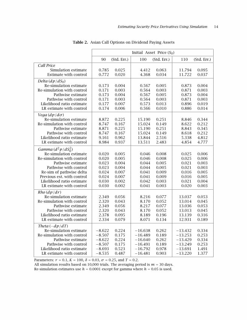
Example 2: Asian Options

In this example derivatives are computed for Asian options, i.e., options on an arithmetic

average price. The payoff of these options is path dependent, that is, the payoff depends not

only on the terminal security price but on all the previous prices that enter into the average.

Closed form expressions for the option price and derivatives are not available for this model.

However, analytical approximations have been developed in Turnbull and Wakeman (1991)

and Ritchken, Sankarasubramanian, and Vijh (1993). Additional analytical results are given in

Geman and Yor (1993). We use this example merely to illustrate simulation results for a path

dependent example. While analytical approaches are available for some Asian option models,

if the stochastic process of the underlying asset is modified slightly, it is straightforward to

modify the simulation estimators but the analytical approaches may not carry through.

We assume that the underlying asset satisfies the stochastic differential equation (1). Let

T be the maturity of the option written on the average of the lastm daily closing prices. Thus,

the average price can be written as S = ∑mi=1 Si/m, where (by a slight abuse of notation) Si is

the price at time ti = T −(m− i)/365.25. For convenience we assume that T > m/365.25, i.e.,

the maturity is greater than the averaging period. The derivative estimators do not change

significantly if this is not the case. When Asian options are initiated, the time until the aver-

aging period begins, t1, is typically much larger than the increment between averaged prices

(which is one day in this example).

The estimators for this example are summarized in Propositions 5 and 6 in Appendix C.

Here theta is defined to be the negative of the derivative of the option price with respect to

maturity for a fixed averaging increment. In other words, a change in T means a change in

the time t1 until averaging begins. All estimators in Propositions 5 and 6 follow from the

same reasoning as the previous ones, though the resulting expressions are more complicated.

In particular, the pathwise estimator for gamma is no longer a constant. Results for this

model are given in Table 2. The results are consistent with those in Example 1, e.g., the point

estimates and standard errors are very close for the pathwise and re-simulation methods. An

exception is gamma, where the standard errors for the pathwise method are smaller than the

re-simulation method. This is due to using a larger value for h, which is necessary because of

machine precision; smaller values of h can give unreliable results. For estimating gamma, a


Table 1. European Call Options on Dividend Paying Assets

Initial Asset Price (S0)

90 (Std. Err.) 100 (Std. Err.) 110 (Std. Err.)

Call PriceExact 1.220 5.126 12.327

Simulation estimate 1.182 0.034 4.993 0.073 12.171 0.107Estimate with control 1.211 0.025 5.073 0.033 12.298 0.023

Delta (dp/dS0)Exact 0.222 0.568 0.844

Re-simulation estimate 0.217 0.005 0.561 0.005 0.844 0.004Re-simulation with control 0.221 0.003 0.566 0.003 0.848 0.002

Pathwise estimate 0.217 0.005 0.561 0.005 0.844 0.004Pathwise with control 0.221 0.003 0.566 0.003 0.848 0.002

Likelihood ratio estimate 0.215 0.008 0.551 0.013 0.817 0.017LR estimate with control 0.220 0.006 0.562 0.008 0.834 0.010

Vega (dp/dσ )Exact 11.946 17.446 11.435




Gamma (d2p/dS20 )

Exact 0.029 0.035 0.019Re-simulation estimate 0.027 0.006 0.048 0.008 0.021 0.005

Re-simulation with control 0.027 0.006 0.048 0.008 0.021 0.005Pathwise estimate 0.029 0.035 0.019


Rho (dp/dr )Exact 3.751 10.344 16.108




Theta (−dp/dT )Exact −8.742 −14.370 −12.415

Re-simulation estimate −8.524 0.191 −14.005 0.203 −11.979 0.245Re-simulation with control −8.701 0.124 −14.226 0.090 −12.240 0.119

Pathwise estimate −8.525 0.191 −14.007 0.203 −11.980 0.245Pathwise with control −8.702 0.124 −14.227 0.090 −12.241 0.119

Likelihood ratio estimate −8.414 0.463 −13.774 0.754 −11.371 1.074LR estimate with control −8.677 0.410 −14.240 0.649 −12.048 0.918

Parameters: r = 0.1, K = 100, δ = 0.03, σ = 0.25, and T = 0.2.All simulation results based on 10,000 trials.Re-simulation estimates use h = 0.0001 except for gamma where h = 0.05 is used.


hybrid method was also tested, i.e., the pathwise estimate of delta was re-simulated.

Example 3: Options with Stochastic Volatility

To illustrate the methods on a model with multiple state variables, derivatives for options

with stochastic volatility are computed in this example. Following Johnson and Shanno (1987)

and Hull and White (1987) we assume that S and σ follow the risk neutralized stochastic

processes:

dSt = St[(r − δ)dt + σt dZt] (19)

dσt = σt[µ dt + ξ dWt] (20)

where Z and W are correlated Brownian motion processes with constant correlation ρ. John-

son and Shanno (1987) present simulation results for this model and Hull and White (1987)

give analytical results for certain special cases and simulation results for other cases. Addi-

tional analytical results for a similar model are given in Heston (1993) and Stein and Stein

(1991). Our aim is to illustrate the simulation methods for derivative estimation on a model

with multiple state variables. Closed form solutions, when available, are generally preferable

to simulation methods because of their computational speed advantage. However, changes to

the stochastic processes (19) and (20) are easily incorporated in the simulation methods, but

the analytical solutions may not be so easily modified.

Our simulation results are based on the following discrete time version of (19)–(20):

Si+1 = Si(1+ (r − δ)∆t + σi√∆t Zi) (21)

σi+1 = σi(1+ µ∆t + ξ√∆t Wi). (22)

In (21)–(22), m is the number of time steps in the discretization, ∆t = T/m, ti = (i/m)T , and

Si and σi are the simulated asset prices and volatilities at time ti, respectively. Also, Zi and

Wi are correlated standard normal random variables. This is a first order Euler approximation

to (19)-(20). See Duffie (1992) for a discussion of discrete approximations to continuous time

models. See Duffie (1992) and Duffie and Glynn (1993) for related convergence issues.

Pathwise and re-simulation results for this example are given in Table 3. Likelihood ratio

estimators are not used because the estimators are substantially more complicated in this

example and because their performance in the earlier examples was not as promising. Pathwise

derivative estimators for this model are given in Proposition 7 in Appendix C. In accordance

with (21)–(22), theta is the negative of the derivative with respect to the maturity T withm held

fixed; thus, d(∆t)/dT = 1/m. In addition to the usual derivatives, sensitivities with respect


Table 2. Asian Call Options on Dividend Paying Assets



Call PriceSimulation estimate 0.785 0.025 4.412 0.063 11.794 0.095

Estimate with control 0.772 0.020 4.368 0.034 11.722 0.037

Delta (dp/dS0)Re-simulation estimate 0.173 0.004 0.567 0.005 0.873 0.004

Re-simulation with control 0.171 0.003 0.564 0.003 0.871 0.003Pathwise estimate 0.173 0.004 0.567 0.005 0.873 0.004

Pathwise with control 0.171 0.003 0.564 0.003 0.871 0.003Likelihood ratio estimate 0.177 0.007 0.573 0.013 0.896 0.019LR estimate with control 0.174 0.006 0.566 0.010 0.886 0.014

Vega (dp/dσ )Re-simulation estimate 8.872 0.225 15.190 0.251 8.846 0.344



Gamma (d2p/dS20 )



Re-sim of pathwise delta 0.024 0.007 0.041 0.009 0.016 0.005Previous est. with control 0.024 0.007 0.041 0.009 0.016 0.005Likelihood ratio estimate 0.030 0.002 0.042 0.003 0.021 0.004LR estimate with control 0.030 0.002 0.041 0.003 0.020 0.003

Rho (dp/dr )Re-simulation estimate 2.349 0.056 8.216 0.077 13.037 0.053



Theta (−dp/dT )Re-simulation estimate −8.622 0.224 −16.638 0.262 −13.432 0.334

Re-simulation with control −8.507 0.175 −16.489 0.189 −13.253 0.253Pathwise estimate −8.622 0.224 −16.640 0.262 −13.429 0.334

Pathwise with control −8.507 0.175 −16.491 0.189 −13.249 0.253Likelihood ratio estimate −8.693 0.523 −16.792 0.978 −13.691 1.491LR estimate with control −8.535 0.487 −16.481 0.903 −13.220 1.377

Parameters: r = 0.1, K = 100, δ = 0.03, σ = 0.25, and T = 0.2.All simulation results based on 10,000 trials. The averaging period is m = 30 days.Re-simulation estimates use h = 0.0001 except for gamma where h = 0.05 is used.


Table 3. Call Options on Dividend Paying Assets with Stochastic Volatility



Call PriceSimulation estimate 1.306 0.039 5.139 0.077 12.286 0.111

Estimate with control 1.285 0.027 5.086 0.032 12.203 0.021

Delta (dp/dS0)Re-simulation estimate 0.220 0.005 0.560 0.005 0.846 0.004


Pathwise with control 0.217 0.003 0.556 0.003 0.843 0.003

Vega (dp/dσ0)Re-simulation estimate 12.229 0.286 17.604 0.314 11.272 0.411



Vega1 (dp/dξ)Re-simulation estimate 0.339 0.025 0.004 0.031 −0.201 0.037

Re-simulation with control 0.332 0.023 −0.003 0.030 −0.209 0.035Pathwise estimate 0.339 0.025 0.004 0.031 −0.201 0.037

Pathwise with control 0.332 0.023 −0.003 0.030 −0.209 0.035

Vega2 (dp/dµ)Re-simulation estimate 0.302 0.008 0.429 0.009 0.273 0.012



Gamma (d2p/dS20 )



Re-sim of pathwise delta 0.024 0.007 0.029 0.008 0.018 0.006Previous est. with control 0.024 0.007 0.029 0.008 0.018 0.006

Rho (dp/dr )Re-simulation estimate 3.687 0.077 10.159 0.098 16.140 0.075



Theta (−dp/dT )Re-simulation estimate −8.996 0.208 −14.191 0.222 −12.037 0.266

Re-simulation with control −8.872 0.130 −14.040 0.099 −11.858 0.126Pathwise estimate −8.996 0.208 −14.193 0.222 −12.039 0.266

Pathwise with control −8.871 0.130 −14.041 0.099 −11.859 0.126

Parameters: r = 0.1, K = 100, δ = 0.03, σ0 = 0.25, T = 0.2, µ = −0.1, ξ = 0.3, and ρ = 0.5.All simulation results based on 10,000 trials. Time is discretized using m = 130 increments.Re-simulation estimates use h = 0.0001 except for gamma where h = 0.05 is used.


to ξ and µ are also computed. Although the estimators are somewhat more complicated than

in the previous example, the results given in Table 3 are similar.

As seen in all three examples, the bias in the re-simulation method is small enough that

it is not an essential concern. Since the computational effort required by the pathwise and

likelihood ratio methods are nearly identical, the difference in standard errors is a strong

argument in favor of the pathwise method. Since the re-simulation method typically requires

much more computational effort than the pathwise method, the nearly identical results for

the two methods also favor the pathwise method.

Control Variates

Variance reduction techniques that apply to the original simulation estimator of a security

price can often be applied to derivative estimators. Among the most powerful tools is the

control variate technique. For consistency we used the same control variate, the terminal

security price, for each of the three examples.4 Next we briefly summarize the control variate

technique. Let D represent an unbiased simulation estimator of the derivative. That is, d =E[D]where d is the true value of the derivative to be estimated. Let ST represent the simulated

terminal price of the security. Since E[ST ] = e(r−δ)T S0, another unbiased estimator of the

derivative is

D′ = D + β(ST − e(r−δ)T S0), (23)

for any β. The parameter β can be chosen to minimize the variance of the estimator D′.

This problem is minβ E[D′ − d]2. An easy computational device for solving this problem is

linear regression. Thus, if the estimators D are regressed on ST , the slope of the regression

line solves the minimization problem. The last step of optimizing over β can significantly

improve the effectiveness of the control variate technique.5 The efficiency of the resulting

estimator D′ depends on the absolute value of the correlation between the original estimator,

D, and the control variate, ST .

5. Conclusions

In this paper two methods for estimating derivatives of security prices using simulation

were presented. The first method uses the dependence of the security payoff on the parameter

of interest. Differentiating this relationship leads, under appropriate conditions, to an unbi-

ased estimator for the derivative of the security price. Since the dependence of the parameter

4 Note that there is always a simple control variable available, namely the random numbers themselves. Weused the terminal security price because it led to a larger reduction in variance.

5 Although this observation is standard in the simulation literature, e.g., §11.4 of Law and Kelton (1991), it hasbeen substantially underutilized in the finance literature.


is identified through the random security payoff, this method is termed the pathwise method.

The second method is based on likelihood ratios. Here the dependence of the underlying

probability density on the parameter of interest is exploited to obtain derivative information.

The main advantage of the direct methods over re-simulation is increased computational

speed. The estimation of n derivatives by the re-simulation method requires n + 1 simula-

tion runs. With the direct methods, the information from a single simulation can be used to

estimate all n derivatives. Solving for the implied value of a parameter given a security price

typically requires many simulation runs. The use of direct methods for estimating deriva-

tives can lead to significant computational savings in these cases. Another advantage is that

the direct methods give unbiased estimates of derivatives, whereas the estimates obtained by

re-simulation are generally biased.

To illustrate and compare the methods, derivatives were computed for a path independent

model, a path dependent model, and a model with multiple state variables. The computational

results indicate that the likelihood ratio method gives significantly larger standard errors than

the pathwise method. The pathwise and re-simulation methods give nearly identical point

estimates and standard errors. Hence, the bias in the re-simulation estimates is not a problem

of practical significance in the examples we considered. Since the results for the pathwise

and re-simulation methods are nearly identical, the computational speed advantage of the

pathwise method is a strong argument in its favor.

6. References

[1] F. Black and M. Scholes, “The Pricing of Options and Corporate Liabilities,” Journal of

Political Economy, Vol. 81, May–June 1973, pp. 637–654.

[2] P. Boyle, “Options: A Monte Carlo Approach,” Journal of Financial Economics, Vol. 4, No. 3,

1977, 323–338.

[3] D.T. Breeden and R.H. Litzenberger, “Prices of State-contingent Claims Implicit in Option

Prices,” Journal of Business, Vol. 51, No. 4, 1978, 621–651.

[4] M. Broadie, “Estimating Duration using Simulation,” Shearson Lehman Hutton research

report, January, 1988.

[5] P. Carr, “Deriving Derivatives of Derivative Securities,” Working paper, Cornell University,

February 1993.

[6] D. Duffie, Dynamic Asset Pricing Theory, Princeton University Press, Princeton, NJ, 1992.

[7] D. Duffie and P. Glynn, “Efficient Monte Carlo Simulation of Security Prices,” Working


paper, Stanford University, March 1993.

[8] P. Franklin, Methods of Advanced Calculus, McGraw-Hill, New York, 1944.

[9] M.C. Fu and J. Hu, “Second Derivative Sample Path Estimators for the GI/G/m Queue,”

Management Science, Vol. 39, No. 3, 1993a, 359–383.

[10] M.C. Fu and J. Hu, “Sensitivity Analysis for Monte Carlo Simulation of Option Pricing,”

Working paper, College of Business and Management, University of Maryland, November

1993b.

[11] H. Geman and M. Yor, “Bessel Processes, Asian options, and perpetuities,” Mathematical

Finance, Vol. 3, No. 4, 1993, 349–375.

[12] P. Glasserman, Gradient Estimation Via Perturbation Analysis, Kluwer Academic Publish-

ers, Norwell, Massachusetts, 1991.

[13] P.W. Glynn, “Likelihood Ratio Estimation: An Overview,” in Proceedings of the 1987 Winter

Simulation Conference, The Society for Computer Simulation, San Diego, California, 1987,

366–375.

[14] P.W. Glynn, “Optimization of Stochastic Systems via Simulation,” in Proceedings of the

1989 Winter Simulation Conference, The Society for Computer Simulation, San Diego,

California, 1989, 90–105.

[15] J.M. Harrison and D. Kreps, “Martingales and Arbitrage in Multiperiod Securities Markets,”

Journal of Economic Theory, Vol. 20, 1979, pp. 381–408.

[16] S.L. Heston, “A Closed-Form Solution for Options with Stochastic Volatility with Appli-

cations to Bond and Currency Options,” Review of Financial Studies, Vol. 6, No. 2, 1993,

327–343.

[17] J. Hull, Options, Futures, and other Derivative Securities, 2nd edition, Prentice-Hall, Engle-

wood Cliffs, New Jersey, 1992.

[18] J. Hull and A. White, “The Pricing of Options on Assets with Stochastic Volatilities,” Journal

of Finance, Vol. 42, No. 2, 1987, 281–300.

[19] H. Johnson and D. Shanno, “Option Pricing when the Variance is Changing,” Journal of

Financial and Quantitative Analysis, Vol. 22, No. 2, 1987, 143–151.

[20] R.A. Jones and R.L. Jacobs, “History Dependent Financial Claims: Monte Carlo Valuation,”

Working paper, Simon Fraser University, 1986.


[21] A.G.Z. Kemna and A.C.F. Vorst, “A Pricing Method for Options Based on Average Asset

Values,” Journal of Banking and Finance, Vol. 14, 1990, 113–129.

[22] A.M. Law and W.D. Kelton, Simulation Modeling and Analysis, 2nd edition, McGraw-Hill,

New York, 1991.

[23] P. L’Ecuyer, “A Unified View of the IPA, SF, and LR Gradient Estimation Techniques,” Man-

agement Science, Vol. 36, No. 11, 1990, 1364–1383.

[24] R.C. Merton, “Theory of Rational Option Pricing,” Bell Journal of Economics and Manage-

ment Science, Vol. 4, 1973, 141–183.

[25] P. Ritchken, L. Sankarasubramanian, and A. Vijh, “The Valuation of Path Dependent Con-

tracts on the Average,” Management Science, Vol. 39, No. 10, 1993, 1202–1213.

[26] R.Y. Rubinstein and A. Shapiro, Discrete Event Systems: Sensitivity Analysis and Stochastic

Optimization by the Score Function Method, John Wiley & Sons, Chichester and New York,

1993.

[27] E.S. Schwartz and W.N. Torous, “Prepayment and the Valuation of Mortgage-Backed Secu-

rities,” Journal of Finance, Vol. 44, No. 2, 1989, 375–392.

[28] C.W. Smith, Jr., C.W. Smithson, and D.S. Wilford, Managing Financial Risk, Harper & Row,

New York, 1990.

[29] E.M. Stein and J.C. Stein, “Stock Price Distributions with Stochastic Volatility: An Analytic

Approach,” Review of Financial Studies, Vol. 4, No. 4, 1991, 727–752.

[30] S.M. Turnbull and L.M. Wakeman, “A Quick Algorithm for Pricing European Average Op-

tions,” Journal of Financial and Quantitative Analysis, Vol. 26, No. 3, 1991, 377–389.

[31] M. Zazanis and R. Suri, “Convergence Rates of Finite-Difference Sensitivity Estimates for

Stochastic Systems,” Operations Research, Vol. 41, No. 4, 1993, 694–703.

Appendix A: General Conditions for Unbiased Estimators

In this appendix, we discuss general conditions for derivative estimators to be unbiased,

giving particular attention to the more delicate case of pathwise estimators.

Let {Xn,n ≥ 0} be a vector-valued state process recording, for example, the price of an

underlying asset, the prevailing interest rate, and any other variables influencing the price of

a derivative security. (Our vectors are column vectors.) The process {Xn}may be a discretiza-

tion of a continuous-time process. We take the discrete-time model as our starting point.


Suppose the discounted payoff associated with a derivative security is given by f(X), where

X = (X1, . . . , XT ), T is the maturity, and f is real-valued. Thus, the price of the security is

p = E[f(X)].Now suppose the state process is a function of a scalar parameter θ ranging over an open

interval Θ. In other words, each Xn is a random function on Θ. For the existence of pathwise

derivatives, we require the following conditions:

(A1) At each θ ∈ Θ,

X′n(θ) ≡ limh→0

Xn(θ + h)−Xn(θ)h

exists with probability 1.

(A2) If Df denotes the set of points at which f is differentiable, then

P(X(θ) ∈ Df) = 1, for all θ ∈ Θ.

Under these conditions, the discounted payoff has a pathwise derivative, given by

ddθf(X(θ)) =

T∑n=1

[∇xnf (X(θ))]tX′n(θ), (24)

where ∇xnf denotes the vector of partial derivatives of f with respect to the components of

Xn, and the superscript t denotes transpose. For this pathwise derivative to be an unbiased

estimator of the derivative of p, we require further conditions:

(A3) There exists a constant kf such that |f(x)− f(y)| ≤ kf‖x−y‖, for all

vectors x,y in the domain of f .

(A4) There exist random variables Kn, n = 1,2, . . ., such that ‖Xn(θ2) −Xn(θ1)‖ ≤ Kn|θ2 − θ1|, for all n, and for all θ1, θ2 ∈ Θ. For each n,

E[Kn] <∞.

Condition (A3) states that f is Lipschitz continuous; condition (A4) states each Xn is

almost surely Lipschitz with an integrable modulus Kn. We now have

Proposition 1: If (A1)–(A4) hold, then at everyθ ∈ Θ, dp(θ)/dθ exists and equals E[df(X)/dθ].

Proof of Proposition 1: Let P(θ) = f(X(θ)); then, as already noted, P ′(θ) exists with prob-

ability 1 if (A1) and (A2) hold. The Lipschitz property is preserved by composition. Hence,


under (A3) and the first part of (A4), P is almost surely Lipschitz continuous; that is, there

exists a random variable KP such that

|P(θ2)− P(θ1)| ≤ KP |θ2 − θ1|, ∀θ1, θ2 ∈ Θ,with probability 1. It follows that for any θ and θ + h in Θ, we have

|P(θ + h)− P(θ)|h

≤ KP .

Moreover, under the second part of (A4), the bound KP has finite expectation (it is bounded

by a linear combination of K1, . . . , KT ), so we may invoke the dominated convergence theorem

to interchange an expectation and the limit as h→ 0 to conclude that p′(θ) exists and equals

E[P ′(θ)]. ♦

The same considerations that arise in justifying the interchange of derivative and integral

for the likelihood ratio method arise in maximum likelihood estimation. Consequently, these

issues have been addressed in the statistical literature, and standard sufficient conditions can

be found in statistics texts. Generally speaking, if the density is a reasonably smooth function

of the parameter in question, the interchange is permissible. For a more detailed examination

of this interchange in the derivative estimation context, see L’Ecuyer (1990).

When a pathwise estimator of a first derivative is Lipschitz continuous, the argument in

Proposition 1 can be applied to show that the pathwise second derivative is also unbiased.

However, we have seen that first derivative estimators often involve indicator functions, mak-

ing them discontinuous. As a result, pathwise estimators of second derivatives do not lend

themselves to a simple, unified treatment along the lines of Proposition 1. The particular

type of “smoothing” required to obtain an unbiased second derivative estimator is problem

dependent. So, we justify our gamma estimators individually in Appendix C. Closely related

approaches are used in other contexts in Fu and Hu (1993a) and in Chapter 7 of Glasserman

(1991).

Appendix B: Optimal Choice of the Parameter Increment in the Re-simulation Method

Let h denote the parameter increment in the re-simulation method. There is an apparent

tradeoff involved in the choice of h. If h is too small, then the variance in the estimates of

the original and perturbed prices can cause a large variance in the estimate of the derivative.

If h is too large, then the nonlinearity of the price as a function of the parameter of interest

can cause a large bias in the derivative estimate. This tradeoff is discussed next. For more


extensive treatments of this topic, see Zazanis and Suri (1993) for the case of independent

re-simulations, and Glynn (1989) for the case of common random numbers. See also Broadie

(1988).

Suppose that the re-simulation method is used to estimate the derivative of the security

price p with respect to a parameter θ. If the function p(θ) is twice continuously differentiable,

Taylor’s theorem implies that the function can be approximated by

p(θ) = p0 + a(θ − θ0)+ b(θ − θ0)2 + o(θ − θ0)2,

where p0 = p(θ0) and a = dp/dθ evaluated at θ = θ0. Suppose that we wish to estimate a. Let

h denote the size of the parameter perturbation and set θ1 = θ0 + h. Let P(θi) = p(θi)+ εi,for i = 0,1, denote the simulation estimator of p(θi). The re-simulation estimator of a is

a = (P(θ1)− P(θ0))/h.6

Suppose that the objective is to minimize the mean squared estimation error. Ignoring

higher order terms,

E[a− a]2 = E[(bh+ ε1 − ε0

h)2]. (25)

For simplicity, suppose that the variances of ε0 and ε1 are equal and denoted by v2. Also, let

ρ denote the correlation of ε0 and ε1 and suppose it is independent of h.

With these assumptions, the parameter increment h∗ that minimizes the mean squared

estimation error is

h∗ = 4

√2v2(1− ρ)

b2. (26)

This follows by expanding the terms in (25) and minimizing (25) over h. Equation (26)

squares with intuition in several regards. As the accuracy of the estimators P(θi) increases (i.e.,

as v2 decreases with additional trials in the simulation) the optimal increment h∗ decreases.

As b2 decreases (i.e., as p(θ) becomes more nearly linear) the optimal increment h∗ increases.

Finally, h∗ decreases as the correlation of the errors approaches one.

Evaluating (25) at h∗ gives E[a − a]2 = 2|bv|√2(1− ρ). This expression illustrates the

importance of using common random numbers for the re-simulation. Using different random

numbers gives a ρ of zero, but using the same stream of random numbers typically gives a

correlation near one, and hence a better derivative estimate.

In our examples, the assumption of equal variances for ε0 and ε1 does not hold precisely,

but more importantly, the assumption of a constant ρ does not hold. In many simulation

6 In terms of derivative estimation alone, it would be better to use a symmetric interval for the finite difference.That is, estimate the derivative at θ0 using the estimators P(θ0 − h/2) and P(θ0 + h/2). However, this approachrequires two additional simulations for each derivative estimate instead of one with the approach in the text.


contexts, e.g., many discrete-event systems, the variance of ε1 − ε0 can be written as hσ 21 (1−

ρ1)+o(h). The optimal increment h in this case is typically smaller than indicated by (26); see

Glynn (1989) for details. In our examples, the variance of ε1 − ε0 can be written as h2σ 21 (1−

ρ1)+o(h2); this always holds under assumptions (A1)–(A4) of Appendix A. This suggests that

the optimal increment in our examples is h∗ = 0+. In practice, we chose h as small as possible,

but large enough that machine precision does not pose a problem in the computations. For

this reason and after some experimentation, we took h = 0.0001 to estimate all derivatives

except gamma, for which h = 0.05 was used.

Appendix C: Summary of Estimators

The proofs of the following propositions are generally similar to the derivations in the

text. Hence, most of the propositions are stated without proof. Where necessary, sketches of

the derivation are given.

Proposition 2 (European call option derivatives):

Delta (dp/dS0): e−δTN(d1(K)) (27)

Vega (dp/dσ ):√Te−δTS0n(d1(K)) (28)

Gamma (d2p/dS20 ): e−δT

n(d1(K))S0σ

√T

(29)

Rho (dp/dr ): KTe−rTN(d2(K)) (30)

Theta (−dp/dT ): − σe−δTS0n(d1(K))

2√T

+ δe−δTS0N(d1(K))− rKe−rTN(d2(K)) (31)

where d1(x) = [ln(S0/x) + (r − δ + 12σ

2)T]/(σ√T) = −d(x) + σ√T , and d2(x) = −d(x).

Also, N(·) is the cumulative distribution function of a standard normal random variable.

Proof of Proposition 2: The European call option value isp = S0e−δTN(d1(K))−e−rTKN(d2(K)),

see, e.g., Black and Scholes (1973) and Merton (1973). The results follow by differentiation. ♦

Proposition 3 (European option pathwise derivative estimators): The following are unbiased

pathwise estimators of the indicated derivatives of European option prices.

Delta (dp/dS0): e−rT1{ST≥K}STS0

(32)

Vega (dp/dσ ): e−rT1{ST≥K}STσ(

ln(ST /S0)− (r − δ− 12σ

2)T)

(33)


Gamma (d2p/dS20 ): e−δT

n(d1(K))S0σ

√T

(34)

Rho (dp/dr ): KTe−rT1{ST≥K} (35)

Theta (−dp/dT ): re−rT max(ST −K,0)− 1{ST≥K}e−rT ST

2T(

ln(ST /S0)+ (r − δ− 12σ

2)T)(36)

Proof of Proposition 3: For each case other than (34), differentiability with probability 1, as

required by conditions (A1)–(A2) of Appendix A follows from (3) and (4): equation (4) shows

that ST is a smooth function of its parameters, and equation (3) shows that P is differentiable

in ST except when ST = K, which occurs with probability 0. For conditions (A3)–(A4), notice

that addition, multiplication by a constant, and the max operation are all Lipschitz functions.

Exponentiation is Lipschitz on bounded intervals and the square root function is Lipschitz

away from the origin. In particular, the discounted payoff P is Lipschitz in a neighborhood of

each of its arguments (since σ > 0 and T > 0). Integrability of the corresponding moduli is

easily verified in each case. The derivation and justification of the gamma estimator are given

in Section 3. ♦

Proposition 4 (European option likelihood ratio derivative estimators): The following are

unbiased likelihood ratio estimators of the indicated derivatives of European option prices.

Delta (dp/dS0): e−rT max(ST −K,0) 1S0 σ 2T

(ln(ST /S0)− (r − δ− 1

2σ2)T

)(37)

Vega (dp/dσ ): e−rT max(ST −K,0)(− d ∂d

∂σ− 1σ)

(38)

Gamma (d2p/dS20 ): e−rT max(ST −K,0)d

2 − dσ√T − 1

S20σ 2T

(39)

Rho (dp/dr ): e−rT max(ST −K,0)(−T + d√T

σ) (40)

Theta (−dp/dT ): e−rT max(ST −K,0)(r + d∂d

∂T+ 1

2T)

(41)

where in (38)–(41) d = d(ST ) = (ln(ST /S0) − (r − δ − 12σ

2)T)/(σ√T), in (38) ∂d/∂σ =

(ln(S0/ST )+(r−δ+12σ

2)T)/(σ 2√T) and in (41) ∂d/∂T = (− ln(ST /S0)−(r−δ−1

2σ2)T)/(2σT 3/2).

Proposition 5 (Asian option pathwise derivative estimators): The following are unbiased

pathwise estimators of the indicated derivatives of Asian option prices.

Delta (dp/dS0): e−rT1{S≥K}SS0

(42)


Vega (dp/dσ ): e−rT1{S≥K}1mσ

m∑i=1

Si(

ln(Si/S0)− (r − δ+ 12σ

2)ti)

(43)

Gamma (d2p/dS20 ): e−rT

( KS0

)2mg(Sm−1,wm,∆tm) (44)

Rho (dp/dr ): 1{S≥K}e−rT ( 1

m

m∑i=1

Siti − T)

(45)

Theta (−dp/dT ): re−rT max(S −K,0)− 1{S≥K}e−rT S

2t1

(ln(S1/S0)+ (r − δ− 1

2σ2)t1

)(46)

where in (44) ∆ti = ti − ti−1, wm = m(K − S) + Sm, g(u,v, t) = n(d(u,v, t))/(vσ√t), and

d(u,v, t) = (ln(v/u)− (r − δ− 12σ

2)t)/(σ√t).

In Table 2 in the text, a hybrid (biased) estimator of gamma is also used. This hybrid

estimator, based on a re-simulation of the pathwise delta estimator, is defined by

Gamma (d2p/dS20 ):

1h(e−rT1{S(S0+h)≥K}

S(S0 + h)S0 + h − e−rT1{S(S0)≥K}

S(S0)S0

). (47)

Proof of Proposition 5: The derivations of vega, theta and gamma are sketched. Note that Sican be written as S0

∏ij=1Xj where ln(Xj) is normally distributed with mean (r −δ− 1

2σ2)∆tj

and variance σ 2∆tj . To compute dS/dσ , the intermediate terms dSi/dσ are needed. Using

d(∏ij=1Xj)dσ

=i∑j=1

(∏k6=j

Xk)dXjdσ

,

dSi/dσ can be written as (Si/σ)(ln(Si/S0) − (r − δ + 12σ

2)ti). The formula for vega now

follows from arguments similar to those in the text.

For theta, recall that the derivative with respect to the maturity means the derivative

with respect to t1, the time until averaging begins. With this understanding, the derivation is

essentially the same as in the European case.

By the same argument used in Section 3 for the European option, gamma can be written as

the product of e−rT (K/S0)2 and the density of S at S = K. There is no closed form expression

for this density, but it can be estimated in the simulation. Conditioning on S1, . . . , Sm−1, we

get, for any x,

P(S ≤ x) = E[P(S ≤ x|S1, . . . , Sm−1)] = E[G(mx −m−1∑j=1

Sj)],


where G is the cumulative lognormal distribution of Sm/Sm−1. Differentiating both sides

and setting x = K, we find that an unbiased estimator of the required density value is

mg(Sm−1,wm,∆tm). ♦Alternative estimators of gamma are obtained through the argument above by condition-

ing on {Sj, j 6= i}, i = 1, . . . ,m− 1. The ith such estimator of the density of S at K is

mg(Si−1,wi,∆ti)g(wi, Si+1,∆ti+1)

g(Si−1, Si+1,∆ti +∆ti+1).

Averaging these m unbiased estimators gives another estimator of gamma:

e−rT( KS0

)2m−1∑i=1

g(Si−1,wi,∆ti)g(wi, Si+1,∆ti+1)g(Si−1, Si+1,∆ti +∆ti+1)

+ g(Sm−1,wm,∆tm).Though theoretically this estimator should have smaller standard error than (44), empirically

we found no significant difference.

Proposition 6 (Asian option likelihood ratio derivative estimators): The following are unbi-

ased likelihood ratio estimators of the indicated derivatives of Asian option prices.

Delta (dp/dS0): e−rT max(S −K,0) 1S0 σ 2∆t1 ( ln(S1/S0)− (r − δ− 1

2σ2)∆t1) (48)

Vega (dp/dσ ): e−rT max(S −K,0)m∑i=1

(− di ∂di∂σ− 1σ)

(49)

Gamma (d2p/dS20 ): e−rT max(S −K,0)d

21 − d1σ

√∆t1 − 1

S20σ 2∆t1 (50)

Rho (dp/dr ): e−rT max(S −K,0)(− T + m∑i=1

di√∆tiσ

)(51)

Theta (−dp/dT ): e−rT max(S −K,0)(r + d1∂d1

∂T+ 1

2∆t1 ) (52)

where ∆ti = ti − ti−1, in (49)–(52) di = (ln(Si/Si−1) − (r − δ − 12σ

2)∆ti)/(σ√∆ti), in (49)

∂di/∂σ = (ln(Si−1/Si)+(r−δ+12σ

2)∆ti)/(σ 2√∆ti), and in (52) ∂d1/∂T is given by (− ln(S1/S0)−

(r − δ− 12σ

2)∆t1)/(2σ∆t13/2).

Proposition 7 (Pathwise derivative estimators of option derivatives with stochastic volatility):

Let ti = (i/m)T and let Si, σi represent the simulated asset price and volatility, respectively,


at time ti. In this discrete time model, the following are unbiased pathwise estimators of the

indicated derivatives of Asian option prices.

Delta (dp/dS0): e−rT1{ST≥K}STS0

(53)

Vega (dp/dσ0): e−rT1{ST≥K}STσ0

m∑i=1

(1− (1+ (r − δ)dt)Si−1

Si

)(54)

Vega1 (dp/dξ): e−rT1{ST≥K}STξ

m∑i=1

(1− (1+ (r − δ)dt)Si−1

Si

)( i−1∑k=1

[1− (1+ µdt)σk−1

σk

])(55)

Vega2 (dp/dµ): e−rT1{ST≥K}ST dtm∑i=2

(1− (1+ (r − δ)dt)Si−1

Si

)( i−1∑k=1

σk−1

σk

)(56)

Gamma (d2p/dS20 ): e−rT

( KS0

)2n( KSmST Sm−1

− (1+ (r − δ)dt)σm−1

√dt

)(57)

Rho (dp/dr ): e−rT1{ST≥K}(− T(ST −K)+ ST dt m∑

i=1

Si−1

Si

)(58)

Theta (−dp/dT ): e−rT1{ST≥K}(r(ST −K)− dSTdT

)(59)

where dt = T/m and n(·) represents the standard normal density function. In (59) the

derivative dST/dT can be evaluated recursively using

dSidT

= dSi−1

dT( SiSi−1

)+ Si−1(r − δm

+ dσi−1

dTZi√dt + σi−1 Zi

2√mT

)(60)

and

dσidT

= dσi−1

dT( σiσi−1

)+ σi−1( µm+ ξWi

2√mT

)(61)

with dS0/dT = 0 and dσ0/dT = 0. In (60) and (61) Zi and Wi are the correlated standard

normal random variables used in the simulation.

In Table 3 in the text, a hybrid (biased) estimator of gamma is also used. This hybrid

estimator, based on a re-simulation of the pathwise delta estimator, is defined by

Gamma (d2p/dS20 ):

1h(e−rT1{S(S0+h)≥K}

ST (S0 + h)S0 + h − e−rT1{S(S0)≥K}

ST (S0)S0

). (62)

Management Science - Columbia Universitymnb2/broadie/Assets/bg-ms-1996.pdf · This paper appeared...

Documents

Transcript of Management Science - Columbia Universitymnb2/broadie/Assets/bg-ms-1996.pdf · This paper appeared...