
Management of uncertainties in numerical aerodynamics
27
Uncertainty quantification and treatment in aircraft design - comparison of approaches Dishi Liu, Alexander Litvinenko, Claudia Schillings, Volker Schulz MUNA Final Workshop October 25, 2012 - DLR Braunschweig research supported by BMWI within the collaborative project MUNA V. Schulz (Universit¨ at Trier) Uncertainty Quantification and Robust Design MUNA - October 25, 2012 1/1
-
Upload
alexander-litvinenko -
Category
Education
-
view
48 -
download
0
Transcript of Management of uncertainties in numerical aerodynamics
Uncertainty quantification and treatment in aircraft design -comparison of approaches
Dishi Liu, Alexander Litvinenko, Claudia Schillings, Volker Schulz
MUNA Final Workshop
October 25, 2012 - DLR Braunschweig
research supported by BMWI within the collaborative project MUNA
V. Schulz (Universitat Trier) Uncertainty Quantification and Robust Design MUNA - October 25, 2012 1 / 1

Test case RAE2822
Test case RAE2822Transonic Euler flowM = 0.73, α = 2◦
Target lift C0L = 0.816
21 design variables193× 33 grid,129 surface pointsDeterministic shapeoptimization problem
miny,p
f (y, p)
s.t. c(y, p) = 0
h(y, p) ≥ 0
V. Schulz (Universitat Trier) Uncertainty Quantification and Robust Design MUNA - October 25, 2012 2 / 1

Test case RAE2822
Geometrical uncertaintiesTransformed Gaussian random field s : Γ×O → R
Assumption:sl ≤ s (x, ζ) ≤ su
Transformation of Gaussian field ψ:
s (x, ζ) = Θ (x, ψ (x, ζ)) = F−1s(x) (Φ (ψ (x, ζ)))
with ψ determined by the mean E (ψ (x, ζ)) = ψ0 (x) and the covariance cov (x, y)
Perturbed geometry:v (x, ζ) = x + s (x, ζ) · n (x) , ∀x ∈ Γ, ζ ∈ O
(cf. e.g. [Matthies, Keese 2003])
V. Schulz (Universitat Trier) Uncertainty Quantification and Robust Design MUNA - October 25, 2012 3 / 1
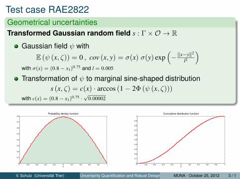
Test case RAE2822Geometrical uncertaintiesTransformed Gaussian random field s : Γ×O → R
Gaussian field ψ with
E (ψ (x, ζ)) = 0 , cov (x, y) = σ(x) σ(y) exp(−‖x−y‖2
l2
)with σ(x) = (0.8− x1)0.75 and l = 0.005
Transformation of ψ to marginal sine-shaped distributions (x, ζ) = c(x) · arccos (1− 2Φ (ψ (x, ζ)))
with c(x) = (0.8− x1)0.75 ·√
0.00002
−1 −0.8 −0.6 −0.4 −0.2 0 0.2 0.4 0.6 0.8 10
0.1
0.2
0.3
0.4
0.5
0.6
0.7
0.8
x
Probability density function
−1 −0.8 −0.6 −0.4 −0.2 0 0.2 0.4 0.6 0.8 10
0.1
0.2
0.3
0.4
0.5
0.6
0.7
0.8
0.9
1
x
Cumulative distribution function
V. Schulz (Universitat Trier) Uncertainty Quantification and Robust Design MUNA - October 25, 2012 3 / 1

Test case RAE2822
Realizations of the Gaussian random field ψ (x, ζ)
0 0.1 0.2 0.3 0.4 0.5 0.6 0.7 0.8 0.9 1−1
−0.5
0
0.5
1
1.5
x
Upper part
0 0.1 0.2 0.3 0.4 0.5 0.6 0.7 0.8 0.9 1−1
−0.5
0
0.5
1
1.5
x
Lower part
Realizations of the transformed random field s (x, ζ)
0 0.1 0.2 0.3 0.4 0.5 0.6 0.7 0.8 0.9 1−2
−1
0
1
2
3x 10
−3
x
Upper part
0 0.1 0.2 0.3 0.4 0.5 0.6 0.7 0.8 0.9 1−2
−1
0
1
2
3x 10
−3
x
Lower part
Resulting perturbed shapes v (x, ζ) = x + s (x, ζ) · n (x)
0 0.1 0.2 0.3 0.4 0.5 0.6 0.7 0.8 0.9 1−0.08
−0.06
−0.04
−0.02
0
0.02
0.04
0.06
0.08
x
y
V. Schulz (Universitat Trier) Uncertainty Quantification and Robust Design MUNA - October 25, 2012 3 / 1
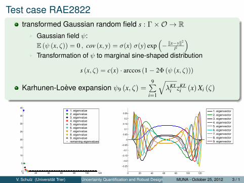
Test case RAE2822transformed Gaussian random field s : Γ×O → R
I Gaussian field ψ:E (ψ (x, ζ)) = 0 , cov (x, y) = σ(x) σ(y) exp
(−‖x−y‖2
l2
)I Transformation of ψ to marginal sine-shaped distribution
s (x, ζ) = c(x) · arccos (1− 2Φ (ψ (x, ζ)))
Karhunen-Loeve expansion ψ9 (x, ζ) =9∑
i=1
√λKL
i zKLi (x) Xi (ζ)
0 20 40 60 80 100 120
−0.25
−0.2
−0.15
−0.1
−0.05
0
0.05
0.1
0.15
0.2
0.25
0 20 40 60 80 100 1200
5
10
15
20
25
30
35
40
1. eigenvector
2. eigenvector
3. eigenvector
4. eigenvector
5. eigenvector
6. eigenvector
7. eigenvector
8. eigenvector
9. eigenvector
1. eigenvalue
2. eigenvalue
3. eigenvalue
4. eigenvalue
5. eigenvalue
6. eigenvalue
7. eigenvalue
8. eigenvalue
9. eigenvalue
remaining eigenvalues
V. Schulz (Universitat Trier) Uncertainty Quantification and Robust Design MUNA - October 25, 2012 3 / 1
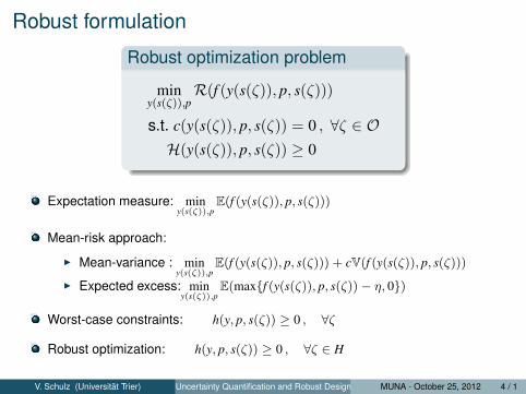
Robust formulation
Robust optimization problem
miny(s(ζ)),p
R(f (y(s(ζ)), p, s(ζ)))
s.t. c(y(s(ζ)), p, s(ζ)) = 0 , ∀ζ ∈ OH(y(s(ζ)), p, s(ζ)) ≥ 0
Expectation measure: miny(s(ζ)),p
E(f (y(s(ζ)), p, s(ζ)))
Mean-risk approach:
I Mean-variance : miny(s(ζ)),p
E(f (y(s(ζ)), p, s(ζ))) + cV(f (y(s(ζ)), p, s(ζ)))I Expected excess: min
y(s(ζ)),pE(max{f (y(s(ζ)), p, s(ζ))− η, 0})
Worst-case constraints: h(y, p, s(ζ)) ≥ 0 , ∀ζ
Robust optimization: h(y, p, s(ζ)) ≥ 0 , ∀ζ ∈ H
V. Schulz (Universitat Trier) Uncertainty Quantification and Robust Design MUNA - October 25, 2012 4 / 1

Summary of the methodology
Quantification One-shot optimization
Approximate the input random field ina finite number of random variables(→ goal-oriented KL expansion)
sd (x, ζ) =d∑
i=1
√λKL
i zKLi (x) Xi (ζ)
Represent the objective functionusing the non-intrusive PC approach+ discretize the probability space tocompute the expansion(→ adaptive sparse grid)
RN(f (p, sd)) =N∑
i=1f (p, si
d)ωi
Solve the lower level problem by adiscretization (reduction) approach
s0 = argminsd
h(p, sd)
Use the generalized version of theone-shot algorithm to solve theresulting robust optimization problem
minyi,p
N∑i=1
f (yi, p, sid)ωi
s.t. c(yi, p, sid) = 0
h(y0, p, s0d) ≥ 0
V. Schulz (Universitat Trier) Uncertainty Quantification and Robust Design MUNA - October 25, 2012 5 / 1
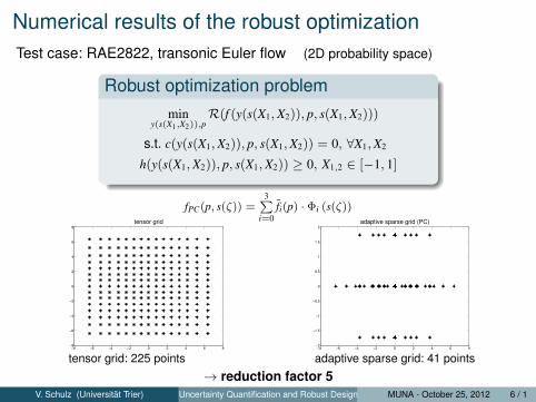
Numerical results of the robust optimizationTest case: RAE2822, transonic Euler flow (2D probability space)
Robust optimization problemmin
y(s(X1,X2)),pR(f (y(s(X1,X2)), p, s(X1,X2)))
s.t. c(y(s(X1,X2)), p, s(X1,X2)) = 0, ∀X1,X2
h(y(s(X1,X2)), p, s(X1,X2)) ≥ 0, X1,2 ∈ [−1, 1]
fPC(p, s(ζ)) =3∑
i=0fi(p) · Φi (s(ζ))
−8 −6 −4 −2 0 2 4 6 8−8
−6
−4
−2
0
2
4
6
8
tensor grid
tensor grid: 225 points−8 −6 −4 −2 0 2 4 6 8
−2
−1.5
−1
−0.5
0
0.5
1
1.5
2
adaptive sparse grid (PC)
adaptive sparse grid: 41 points
→ reduction factor 5V. Schulz (Universitat Trier) Uncertainty Quantification and Robust Design MUNA - October 25, 2012 6 / 1
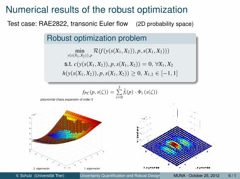
Numerical results of the robust optimizationTest case: RAE2822, transonic Euler flow (2D probability space)
Robust optimization problemmin
y(s(X1,X2)),pR(f (y(s(X1,X2)), p, s(X1,X2)))
s.t. c(y(s(X1,X2)), p, s(X1,X2)) = 0, ∀X1,X2
h(y(s(X1,X2)), p, s(X1,X2)) ≥ 0, X1,2 ∈ [−1, 1]
fPC(p, s(ζ)) =3∑
i=0fi(p) · Φi (s(ζ))
−3
−2
−1
0
1
2
3
−3
−2
−1
0
1
2
32
3
4
5
6
7
8
x 10−3
1. eigenvector
polynomial chaos expansion of order 3
2. eigenvector
V. Schulz (Universitat Trier) Uncertainty Quantification and Robust Design MUNA - October 25, 2012 6 / 1
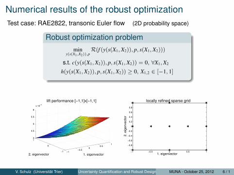
Numerical results of the robust optimizationTest case: RAE2822, transonic Euler flow (2D probability space)
Robust optimization problemmin
y(s(X1,X2)),pR(f (y(s(X1,X2)), p, s(X1,X2)))
s.t. c(y(s(X1,X2)), p, s(X1,X2)) = 0, ∀X1,X2
h(y(s(X1,X2)), p, s(X1,X2)) ≥ 0, X1,2 ∈ [−1, 1]
−1−0.5
00.5
1
−1
0
14
4.5
5
5.5
6
x 10−3
1. eigenvector
lift performance [−1,1]x[−1,1]
2. eigenvector−1 −0.5 0 0.5 1
−1
−0.8
−0.6
−0.4
−0.2
0
0.2
0.4
0.6
0.8
1
1. eigenvector
2. eig
envecto
r
locally refined sparse grid
V. Schulz (Universitat Trier) Uncertainty Quantification and Robust Design MUNA - October 25, 2012 6 / 1

Numerical results of the robust optimizationTest case: RAE2822, transonic Euler flow (2D probability space)
Measure of robustness Statistics
fnominal E Var EEE η=4.15·10−3 EEE η=4.4·10−3
single-setpoint 3.45 · 10−3 4.47 · 10−3 1.13 · 10−6 5.20 · 10−4 4.03 · 10−4
E 3.75 · 10−3 4.15 · 10−3 3.57 · 10−7 1.94 · 10−4 1.19 · 10−4
E + 103 · Var 3.81 · 10−3 4.10 · 10−3 2.55 · 10−7 1.73 · 10−4 9.90 · 10−5
E + 104 Var 4.04 · 10−3 4.33 · 10−3 8.91 · 10−8 2.18 · 10−4 9.13 · 10−5
E + 105 · Var 5.93 · 10−3 6.06 · 10−3 2.22 · 10−8 1.91 · 10−3 1.66 · 10−3
EEE η=4.15·10−3 3.77 · 10−3 4.13 · 10−3 1.26 · 10−7 1.33 · 10−4 6.41 · 10−5
EEE η=4.40·10−3 3.81 · 10−3 4.16 · 10−3 1.09 · 10−7 1.33 · 10−4 6.09 · 10−5
0 0.1 0.2 0.3 0.4 0.5 0.6 0.7 0.8 0.9 1−0.08
−0.06
−0.04
−0.02
0
0.02
0.04
0.06
x
y
single−setpoint
E
E+103 Var
E+104 Var
E+105 Var
EE η=0.00415
EE η=0.0044
V. Schulz (Universitat Trier) Uncertainty Quantification and Robust Design MUNA - October 25, 2012 7 / 1

Numerical results of the robust optimizationTest case: RAE2822, transonic Euler flow (9D probability space)
Adaptive selection of the KL basis
−1 −0.8 −0.6 −0.4 −0.2 0 0.2 0.4 0.6 0.8 1
4.4
4.6
4.8
5
5.2
5.4x 10
−3
perturbations
dra
g (
obje
ctive function)
1. eigenvector, indicator: 4.73 10−04
2. eigenvector, indicator: 4.37 10−04
3. eigenvector, indicator:−1.21 10−04
4. eigenvector, indicator: 1.14 10−04
5. eigenvector, indicator:−1.25 10−04
6. eigenvector, indicator: 1.33 10−05
7. eigenvector, indicator: 2.05 10−05
8. eigenvector, indicator:−1.33 10−05
9. eigenvector, indicator: 6.23 10−06
6. - 9. eigenvectors have no impact on the drag performance
→ reduction of the dimension
V. Schulz (Universitat Trier) Uncertainty Quantification and Robust Design MUNA - October 25, 2012 8 / 1

Numerical results of the robust optimizationTest case: RAE2822, transonic Euler flow (9D probability space)
Adaptive selection of the KL basis
−1 −0.8 −0.6 −0.4 −0.2 0 0.2 0.4 0.6 0.8 1−5
−4
−3
−2
−1
0
1
2
3
4x 10
−3
perturbations
lift (inequalit
y c
onstr
ain
t)
1. eigenvector, indicator: 4.60 10−3
2. eigenvector, indicator: −1.67 10−3
3. eigenvector, indicator: 1.19 10−3
4. eigenvector, indicator: −8.93 10−4
5. eigenvector, indicator: 9.00 10−4
6. eigenvector, indicator: −5.64 10−4
7. eigenvector, indicator: −1.05 10−4
8. eigenvector, indicator: 1.47 10−4
9. eigenvector, indicator: −5.88 10−5
6. - 9. eigenvectors have no impact on the drag performance
→ reduction of the dimension
V. Schulz (Universitat Trier) Uncertainty Quantification and Robust Design MUNA - October 25, 2012 8 / 1
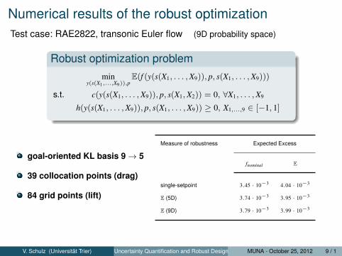
Numerical results of the robust optimizationTest case: RAE2822, transonic Euler flow (9D probability space)
Robust optimization problemmin
y(s(X1,...,X9)),pE(f (y(s(X1, . . . ,X9)), p, s(X1, . . . ,X9)))
s.t. c(y(s(X1, . . . ,X9)), p, s(X1,X2)) = 0, ∀X1, . . . ,X9
h(y(s(X1, . . . ,X9)), p, s(X1, . . . ,X9)) ≥ 0, X1,...,9 ∈ [−1, 1]
goal-oriented KL basis 9→ 5
39 collocation points (drag)
84 grid points (lift)
Measure of robustness Expected Excess
fnominal E
single-setpoint 3.45 · 10−3 4.04 · 10−3
E (5D) 3.74 · 10−3 3.95 · 10−3
E (9D) 3.79 · 10−3 3.99 · 10−3
V. Schulz (Universitat Trier) Uncertainty Quantification and Robust Design MUNA - October 25, 2012 9 / 1

Numerical results of the robust optimizationTest case: RAE2822, transonic Euler flow (9D probability space)
Robust optimization problemmin
y(s(X1,...,X9)),pE(f (y(s(X1, . . . ,X9)), p, s(X1, . . . ,X9)))
s.t. c(y(s(X1, . . . ,X9)), p, s(X1,X2)) = 0, ∀X1, . . . ,X9
h(y(s(X1, . . . ,X9)), p, s(X1, . . . ,X9)) ≥ 0, X1,...,9 ∈ [−1, 1]
0 0.1 0.2 0.3 0.4 0.5 0.6 0.7 0.8 0.9 1−0.08
−0.06
−0.04
−0.02
0
0.02
0.04
0.06
x
y
robust optimization (5D)robust optimization (9D)
V. Schulz (Universitat Trier) Uncertainty Quantification and Robust Design MUNA - October 25, 2012 9 / 1

Uncertainty quantification - objective
We estimate some statistics of CL and CD under the uncertainty ofairfoil geometry.
Target statistics:
Mean, µ`, µd
Standard deviations, σ`, σd
Exceedance probabilities,
P`,κ = Pro{CL < µ` − κ · σ`} andPd,κ = Pro{CD > µd − κ · σd} with κ = 2, 3.
Objective:To identify an efficient method for estimating the statistics in thiskind of problem.
V. Schulz (Universitat Trier) Uncertainty Quantification and Robust Design MUNA - October 25, 2012 10 / 1

Uncertainty quantification - comparison of methodsTo compare the efficiency of methods in estimating the statistics.
Methods:
gradient-employingI gradient-assisted point-collocation polynomial chaos (GAPC)I gradient-assisted radial basis function (GARBF)I gradient-enhanced Kriging (GEK)
not gradient-employingI quasi-Monte Carlo quadrature (QMC), with low discrepancy sequenceI polynomial chaos (PC), with coefficients estimated by sparse grid quadrature
Criteria: computation cost for a certain accuracy in the statistics.
Cost: measured in elapse time-penalized sample number MM = 2N for gradient-employing methodM = N for others
Accuracy: judged by comparing with a reference statistics obtained by a QMC ofN = 5× 10⁵.
V. Schulz (Universitat Trier) Uncertainty Quantification and Robust Design MUNA - October 25, 2012 11 / 1

Uncertainty quantification - numerical results
50 100 150 2001e−06
1e−05
1e−04
1e−03
1e−02
1e−01
1e+00
M
Err
or
On estimating the mean of CL
QMCPCGEKGAPCGARBF
50 100 150 2001e−06
1e−04
1e−02
1e+00
ME
rro
r
On estimating the stdv of CL
QMCPCGEKGAPCGARBF
Abbildung: Comparison on estimating the mean and standard deviation of CL
V. Schulz (Universitat Trier) Uncertainty Quantification and Robust Design MUNA - October 25, 2012 12 / 1
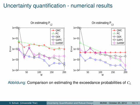
Uncertainty quantification - numerical results
50 100 150 2001e−04
1e−03
1e−02
1e−01
1e+00
M
Err
or
On estimating Pl,2
QMCPCGEKGAPCGARBF
50 100 150 2001e−04
1e−03
1e−02
1e−01
1e+00
ME
rro
r
On estimating Pl,3
QMCPCGEKGAPCGARBF
Abbildung: Comparison on estimating the exceedance probabilities of CL
V. Schulz (Universitat Trier) Uncertainty Quantification and Robust Design MUNA - October 25, 2012 13 / 1

Uncertainty quantification - numerical results
50 100 150 2001e−08
1e−06
1e−04
1e−02
M
Err
or
On estimating the mean of CD
QMCPCGEKGAPCGARBF
50 100 150 200
1e−06
1e−04
1e−02
M
On estimating the stdv of CD
QMCPCGEKGAPCGARBF
Abbildung: Comparison on estimating the mean and standard deviation of CD
V. Schulz (Universitat Trier) Uncertainty Quantification and Robust Design MUNA - October 25, 2012 14 / 1
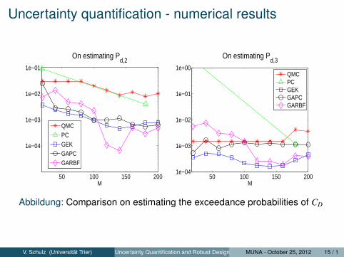
Uncertainty quantification - numerical results
50 100 150 200
1e−04
1e−03
1e−02
1e−01
M
On estimating Pd,2
QMCPCGEKGAPCGARBF
50 100 150 2001e−04
1e−03
1e−02
1e−01
1e+00
M
On estimating Pd,3
QMCPCGEKGAPCGARBF
Abbildung: Comparison on estimating the exceedance probabilities of CD
V. Schulz (Universitat Trier) Uncertainty Quantification and Robust Design MUNA - October 25, 2012 15 / 1
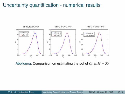
Uncertainty quantification - numerical results
0.79 0.8 0.81 0.82 0.830
20
40
60
80
100
CL
pdf of CL by GEK, M=50
reference pdfpdf by GEK
0.79 0.8 0.81 0.82 0.830
20
40
60
80
100
CL
pdf of CL by GAPC, M=50
reference pdfpdf by GAPC
0.79 0.8 0.81 0.82 0.830
20
40
60
80
100
CL
pdf of CL by GARBF, M=50
reference pdfpdf by GARBF
Abbildung: Comparison on estimating the pdf of CL at M = 50
V. Schulz (Universitat Trier) Uncertainty Quantification and Robust Design MUNA - October 25, 2012 16 / 1

Uncertainty quantification - numerical results
0.003 0.004 0.005 0.006 0.007 0.008 0.0090
100
200
300
400
500
600
CD
pdf of CD
by GEK, M=50
reference pdfpdf by GEK
0.003 0.004 0.005 0.006 0.007 0.008 0.0090
100
200
300
400
500
600
CD
pdf of CD
by GAPC, M=50
reference pdfpdf by GAPC
0.003 0.004 0.005 0.006 0.007 0.008 0.0090
100
200
300
400
500
600
CD
pdf of CD
by GARBF, M=50
reference pdfpdf by GARBF
Abbildung: Comparison on estimating the pdf of CD at M = 50
V. Schulz (Universitat Trier) Uncertainty Quantification and Robust Design MUNA - October 25, 2012 17 / 1

Uncertainty quantification - numerical results
pdf of CL and CD by polynomial Chaos expansion (PC)PC expansion is computed on the sparse Gauss-Hermite grid (SGH)with 19 nodes ( polynomial order p = 1).
Abbildung: Comparison of pdf computed by PC and the reference pdf, p = 1,19 TAU evaluations.
V. Schulz (Universitat Trier) Uncertainty Quantification and Robust Design MUNA - October 25, 2012 18 / 1

Uncertainty quantification - conclusion
Conclusion:
Gradient-employing surrogate methods outperform the others
GEK seems more efficient than other gradient-employingmethods, especially when M is small, and when estimating the“far-end” exceedance probability and the pdf.
Since PC only has two data point, its performance in thiscomparison may not indicate its asymptotic capacity.
V. Schulz (Universitat Trier) Uncertainty Quantification and Robust Design MUNA - October 25, 2012 19 / 1

Summary
Summary:An aerodynamic testcase of geometric uncertainties is setup forjoint research on UQ and RD.
Karhunen-Loeve expansion proved an effect tool to reduce thenumber of variables.
Robust design is implemented on the testcase with differentrobust measures and numerical methods.
Uncertainty quantification methods are applied on the testcaseand their efficiency compared.
V. Schulz (Universitat Trier) Uncertainty Quantification and Robust Design MUNA - October 25, 2012 20 / 1


