MAKING CHOICES IN MULTI-DIMENSIONAL PARAMETER SPACES CHOICES IN MULTI-DIMENSIONAL PARAMETER SPACES...
185
MAKING CHOICES IN MULTI-DIMENSIONAL PARAMETER SPACES by Steven Bergner MSc, Otto-von-Guericke University of Magdeburg, 2003 a Thesis submitted in partial fulfillment of the requirements for the degree of Doctor of Philosophy in the School of Computing Science Faculty of Applied Sciences c Steven Bergner 2011 SIMON FRASER UNIVERSITY Fall 2011 All rights reserved. However, in accordance with the Copyright Act of Canada, this work may be reproduced, without authorization, under the conditions for Fair Dealing. Therefore, limited reproduction of this work for the purposes of private study, research, criticism, review and news reporting is likely to be in accordance with the law, particularly if cited appropriately.
Transcript of MAKING CHOICES IN MULTI-DIMENSIONAL PARAMETER SPACES CHOICES IN MULTI-DIMENSIONAL PARAMETER SPACES...
MAKING CHOICES IN MULTI-DIMENSIONAL
PARAMETER SPACES
by
Steven Bergner
MSc, Otto-von-Guericke University of Magdeburg, 2003
a Thesis submitted in partial fulfillment
of the requirements for the degree of
Doctor of Philosophy
in the
School of Computing Science
Faculty of Applied Sciences
c© Steven Bergner 2011
SIMON FRASER UNIVERSITY
Fall 2011
All rights reserved.
However, in accordance with the Copyright Act of Canada, this work may be reproduced, without
authorization, under the conditions for Fair Dealing. Therefore, limited reproduction of this work
for the purposes of private study, research, criticism, review and news reporting is likely to be in
accordance with the law, particularly if cited appropriately.

APPROVAL
Name: Steven Bergner
Degree: Doctor of Philosophy
Title of Thesis: Making choices in multi-dimensional parameter spaces
Examining Committee: Dr. Mark Drew
Chair
Dr. Torsten Moller, Senior Supervisor
Professor of Computing Science
Dr. Derek Bingham, Supervisor
Associate Professor — Industrial Statistics
Dr. Steven J. Ruuth, Internal Examiner
Professor of Applied and Computational Mathematics
Dr. Min Chen, External Examiner
Professor of Scientific Visualization
University of Oxford
Date Approved:
ii
thesis
Typewritten Text
16 December 2011

Last revision: Spring 09
Declaration of Partial Copyright Licence The author, whose copyright is declared on the title page of this work, has granted to Simon Fraser University the right to lend this thesis, project or extended essay to users of the Simon Fraser University Library, and to make partial or single copies only for such users or in response to a request from the library of any other university, or other educational institution, on its own behalf or for one of its users.
The author has further granted permission to Simon Fraser University to keep or make a digital copy for use in its circulating collection (currently available to the public at the “Institutional Repository” link of the SFU Library website <www.lib.sfu.ca> at: <http://ir.lib.sfu.ca/handle/1892/112>) and, without changing the content, to translate the thesis/project or extended essays, if technically possible, to any medium or format for the purpose of preservation of the digital work.
The author has further agreed that permission for multiple copying of this work for scholarly purposes may be granted by either the author or the Dean of Graduate Studies.
It is understood that copying or publication of this work for financial gain shall not be allowed without the author’s written permission.
Permission for public performance, or limited permission for private scholarly use, of any multimedia materials forming part of this work, may have been granted by the author. This information may be found on the separately catalogued multimedia material and in the signed Partial Copyright Licence.
While licensing SFU to permit the above uses, the author retains copyright in the thesis, project or extended essays, including the right to change the work for subsequent purposes, including editing and publishing the work in whole or in part, and licensing other parties, as the author may desire.
The original Partial Copyright Licence attesting to these terms, and signed by this author, may be found in the original bound copy of this work, retained in the Simon Fraser University Archive.
Simon Fraser University Library Burnaby, BC, Canada

STATEMENT OF ETHICS APPROVAL
The author, whose name appears on the title page of this work, has obtained, for the research described in this work, either:
(a) Human research ethics approval from the Simon Fraser University Office of Research Ethics,
or
(b) Advance approval of the animal care protocol from the University Animal Care Committee of Simon Fraser University;
or has conducted the research
(c) as a co-investigator, collaborator or research assistant in a research project approved in advance,
or
(d) as a member of a course approved in advance for minimal risk human research, by the Office of Research Ethics.
A copy of the approval letter has been filed at the Theses Office of the University Library at the time of submission of this thesis or project.
The original application for approval and letter of approval are filed with the relevant offices. Inquiries may be directed to those authorities.
Simon Fraser University Library
Simon Fraser University Burnaby, BC, Canada
Last update: Spring 2010
Abstract
Visualization techniques are key to leveraging human experience, knowledge, and intuition
when establishing a connection between computational models and real world systems. At
this interface my dissertation enables effective choices of parameter configurations for dif-
ferent levels of user involvement.
Based on a characterization of several domains of computer experimentation that include
a model of biological aggregations, image segmentation methods, and rendering algorithms,
I derive a set of requirements to propose paraglide — a framework for user-driven analysis of
parameter effects. One outcome of the workflow I suggest is a partitioning of the continuous
space of model configurations into distinct regions of homogenous system behaviour.
To facilitate progressive exploration of a parameter region, I develop a space-filling sam-
pling method by constructing point lattices that contain rotated and scaled versions of
themselves. All levels of resolution share a single type of Voronoi polytope, whose volume
grows independently of the dimensionality by a chosen integer factor as low as 2.
To optimize rendering time while ensuring image quality when viewing data in a 3-
dimensional volume, I perform a Fourier domain analysis of the effect of composing two
functions. Based on this, I relax a previous lower bound for a sufficient sampling frequency
and apply it to adaptively choose the numerical integration step size in raycasting.
By assigning optical properties to data using a spectral light model, it becomes possible
to improve physical realism and to create colour effects that scale the level of distinguishable
detail in a visualization. To help modellers to cope with the freedom in a large design space
of synthetic lights and materials, I devise a method that generates a palette of presets that
globally optimize user-specified criteria and regularization. This is augmented with two
alternative user interfaces to unobtrusively choose a desired mixture.
iii

Acknowledgments
On my way through graduate school I had the luck to cross paths with many remarkable
people. I am grateful to my supervisors Torsten Moller and Derek Bingham for inspiring
discussions, constructive input, and ongoing support. Min Chen and Steve Ruuth deserve
credit for their willingness to examine my thesis on rather short notice and still providing
very good feedback.
The folks at the Graphics, Usability, and Visualization laboratory (GrUVi) at Simon
Fraser University made this an inspiring and fun place to work. While I had many inspiring
discussions throughout the years in the lab, I would in particular like to acknowledge Ramsay
Dyer, Alireza Entezari, Ahmed Saad, Tai Meng, Zahid Hossain, and Tom Torsney-Weir for
their input and collaborations. In particular, I would like to thank Usman Alim, Niklas
Rober, and Nhi Nguyen for proof reading parts of my thesis.
There are also several people beyond the lab that I had the honour to learn from during
different stages of my research: Mark Drew, Dave Muraki, Thierry Blu, Dimitri Van De
Ville, Melanie Tory, Tamara Munzner, Michael Sedlmair, and Stephen Ingram.
Also, I would like to thank past students for their great work that they did under my
(co-)supervision (or despite of it): Vincent Cua, Vladimir Kim, Rishabh Iyer, Matt Crider,
Theresa Sanchez, and Sareh Nabi Abdolyousefi.
Apart from proof reading, I am indebted to Nhi Nguyen for always having an open ear
and for being and amazing friend and partner in all regards beyond grad school.
Last, but not least, none of this journey would have been possible without the encour-
agement and support of my parents and my whole family to whom I would like to extend
my deepest gratitude.
iv
Contents
Approval ii
Abstract iii
Acknowledgments iv
Contents v
List of Tables ix
List of Figures x
1 Connecting formal and real systems 1
1.1 Contributions of this dissertation . . . . . . . . . . . . . . . . . . . . . . . . . 3
1.2 Problem domains that require parameter tuning . . . . . . . . . . . . . . . . 4
1.2.1 Mathematical modelling: Collective behaviour in biological aggregations 5
1.2.2 Bio-medical imaging: Segmentation algorithm . . . . . . . . . . . . . 7
1.2.3 Engineering: Fuel cells . . . . . . . . . . . . . . . . . . . . . . . . . . 7
1.2.4 Visualization: Scene setup and rendering algorithm configuration . . . 9
1.3 Task structure . . . . . . . . . . . . . . . . . . . . . . . . . . . . . . . . . . . 12
1.4 Data abstraction . . . . . . . . . . . . . . . . . . . . . . . . . . . . . . . . . . 15
2 Acquisition and visualization of multi-variate data 19
2.1 Effects of dimensionality . . . . . . . . . . . . . . . . . . . . . . . . . . . . . 20
2.2 Quadrature error . . . . . . . . . . . . . . . . . . . . . . . . . . . . . . . . . . 23
2.3 Discretization of multi-dimensional functions . . . . . . . . . . . . . . . . . . 25
2.3.1 Useful concepts for metric data representation . . . . . . . . . . . . . 25
v

2.3.2 Experimental design . . . . . . . . . . . . . . . . . . . . . . . . . . . . 29
2.3.3 Figures of merit: Packing and covering radii, density, and thickness . . 31
2.3.4 Optimal packing and bounds by Minkowski and Zador . . . . . . . . 32
2.4 Visual interfaces for multi-variate computer model data . . . . . . . . . . . . 34
2.4.1 Computational modelling tasks . . . . . . . . . . . . . . . . . . . . . 36
2.4.2 Reconstruction and refinement of spatial data . . . . . . . . . . . . . . 39
2.4.3 Direct volume rendering . . . . . . . . . . . . . . . . . . . . . . . . . 40
2.4.4 Visualization systems for discrete multi-variate data . . . . . . . . . . 41
3 Sampling lattices with low-rate refinement 43
3.1 Change of lattice basis and similarity . . . . . . . . . . . . . . . . . . . . . . . 44
3.2 Construction of sampling lattices with low-rate rotational dilation . . . . . . 47
3.2.1 Constructing rotational dilation matrices . . . . . . . . . . . . . . . . 49
3.2.2 Characteristic polynomial of a scaled rotation matrix in Rn . . . . . . 50
3.2.3 Construction algorithm . . . . . . . . . . . . . . . . . . . . . . . . . . 52
3.3 Further dimensions and subsampling ratios . . . . . . . . . . . . . . . . . . . 53
4 A sampling bound for composed functions 57
4.1 Frequency domain analysis . . . . . . . . . . . . . . . . . . . . . . . . . . . . 59
4.1.1 Visual inspection of the frequency transfer kernel K(ω,ν) . . . . . . . 60
4.1.2 Determining the boundary of the cone . . . . . . . . . . . . . . . . . 62
4.1.3 Error analysis . . . . . . . . . . . . . . . . . . . . . . . . . . . . . . . . 64
4.1.4 Limits of the model . . . . . . . . . . . . . . . . . . . . . . . . . . . . 65
4.1.5 Relationship to Carson’s rule . . . . . . . . . . . . . . . . . . . . . . . 65
4.2 Application to volume rendering . . . . . . . . . . . . . . . . . . . . . . . . . 66
4.3 Discussion and outlook . . . . . . . . . . . . . . . . . . . . . . . . . . . . . . . 69
5 Designing a palette for spectral lighting 71
5.1 Related work . . . . . . . . . . . . . . . . . . . . . . . . . . . . . . . . . . . . 74
5.1.1 Previous approaches to constructing spectra . . . . . . . . . . . . . . . 75
5.1.2 Linear light models . . . . . . . . . . . . . . . . . . . . . . . . . . . . 76
5.1.3 Accuracy . . . . . . . . . . . . . . . . . . . . . . . . . . . . . . . . . . 78
5.2 Designing spectra . . . . . . . . . . . . . . . . . . . . . . . . . . . . . . . . . . 79
5.3 Matrix formulation . . . . . . . . . . . . . . . . . . . . . . . . . . . . . . . . 80
vi
5.3.1 Combined optimization function . . . . . . . . . . . . . . . . . . . . . 82
5.3.2 Free metamers . . . . . . . . . . . . . . . . . . . . . . . . . . . . . . . 83
5.4 Evaluation and visual results . . . . . . . . . . . . . . . . . . . . . . . . . . . 84
5.4.1 Example palette design . . . . . . . . . . . . . . . . . . . . . . . . . . 85
5.4.2 Design error with respect to number of constraints . . . . . . . . . . . 85
5.4.3 Spectral surface graphics . . . . . . . . . . . . . . . . . . . . . . . . . 89
5.4.4 Rendering volumes interactively . . . . . . . . . . . . . . . . . . . . . 90
5.5 Discussion and conclusions . . . . . . . . . . . . . . . . . . . . . . . . . . . . . 91
5.5.1 Future directions . . . . . . . . . . . . . . . . . . . . . . . . . . . . . . 93
5.5.2 Conclusions . . . . . . . . . . . . . . . . . . . . . . . . . . . . . . . . 94
6 Interactive parameter space partitioning 95
6.1 Background . . . . . . . . . . . . . . . . . . . . . . . . . . . . . . . . . . . . 96
6.1.1 Interactive parameter adjustment in computer experiments . . . . . . 97
6.1.2 Parameter space partitioning . . . . . . . . . . . . . . . . . . . . . . . 98
6.1.3 Unfulfilled design requirements . . . . . . . . . . . . . . . . . . . . . . 99
6.2 Design of the paraglide system . . . . . . . . . . . . . . . . . . . . . . . . . . 99
6.2.1 System components . . . . . . . . . . . . . . . . . . . . . . . . . . . . 100
6.2.2 Browsing computed data . . . . . . . . . . . . . . . . . . . . . . . . . 102
6.2.3 Representing a region of interest . . . . . . . . . . . . . . . . . . . . . 105
6.2.4 Non-linear screen mappings . . . . . . . . . . . . . . . . . . . . . . . . 107
6.3 Excursion: Steering a multi-dimensional cursor . . . . . . . . . . . . . . . . . 109
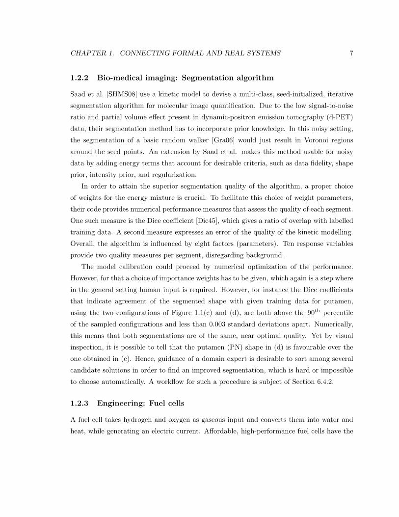
6.3.1 A light dial to control additive mixtures . . . . . . . . . . . . . . . . 109
6.3.2 Enabling simultaneous parameter adjustments using a mixing board . 111
6.4 Validation of paraglide in different use cases . . . . . . . . . . . . . . . . . . . 118
6.4.1 Movement patterns of biological aggregations . . . . . . . . . . . . . . 118
6.4.2 Bio-medical imaging: Tuning image segmentation parameters . . . . 120
6.4.3 Fuel cell stack prototyping . . . . . . . . . . . . . . . . . . . . . . . . 123
6.5 Discussion and future work . . . . . . . . . . . . . . . . . . . . . . . . . . . . 124
7 Discussion and conclusion 128
7.1 Conclusion . . . . . . . . . . . . . . . . . . . . . . . . . . . . . . . . . . . . . 131
vii

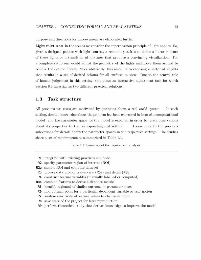
List of Tables
1.1 Summary of the requirement analysis. . . . . . . . . . . . . . . . . . . . . . . 12
7.1 Summary of thesis contributions where the level of user involvement decreases
and the inclusion of theoretical analysis increases from top to bottom, with
rows corresponding to different chapters in the order 6, 5, 4, and 3. . . . . . 130
ix

List of Figures
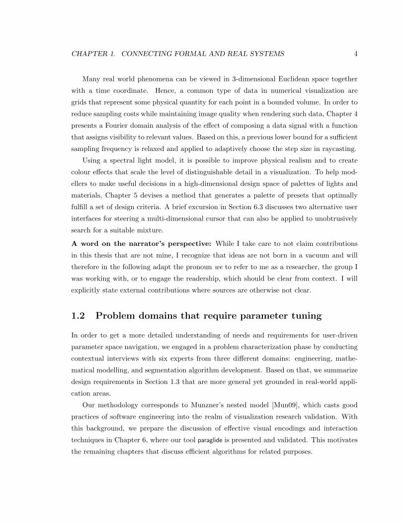
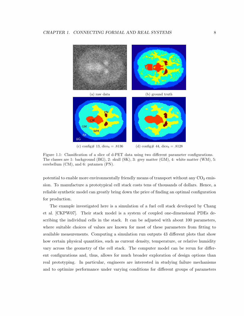
1.1 Classification of a slice of d-PET data using two different parameter config-
urations. The classes are 1: background (BG), 2: skull (SK), 3: grey matter
(GM), 4: white matter (WM), 5: cerebellum (CM), and 6: putamen (PN). . 8
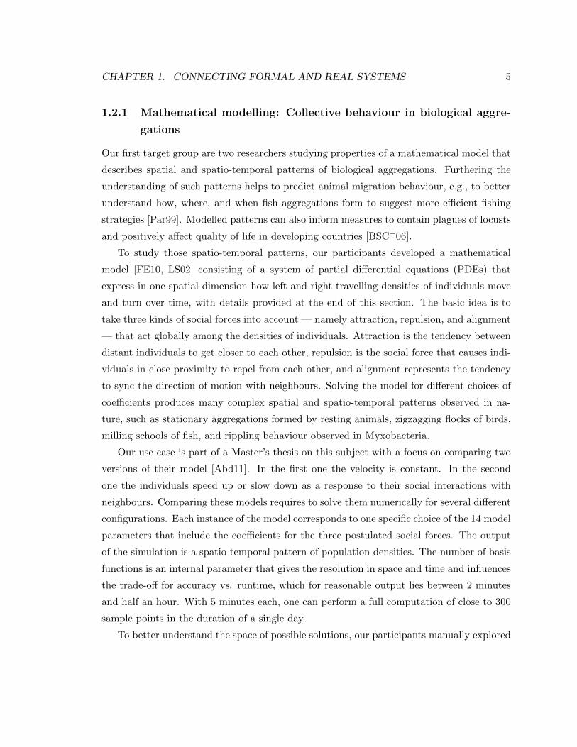
1.2 (a) SPloM view evaluation of the effect of value reconstruction filter (top
row) and sampling distance (bottom row). The columns show different image
comparison metrics by comparing with a best possible ground ’truth’ image
(b) showing the 643 hipiph data set using a transfer function that includes
smooth and sharp opacity transitions. Value filters are sorted by order of
approximation (ef:1,2,3,4) and, within each order, by degree of smoothness
(c:1,2,3) [MMMY97]. The sampling step size along a ray is colour coded
from bottom to top / blue to orange for [1/200, 1/32, 1/16, 1/8, 1/4, 1/2, 1]
grid spacing units. . . . . . . . . . . . . . . . . . . . . . . . . . . . . . . . . . 10
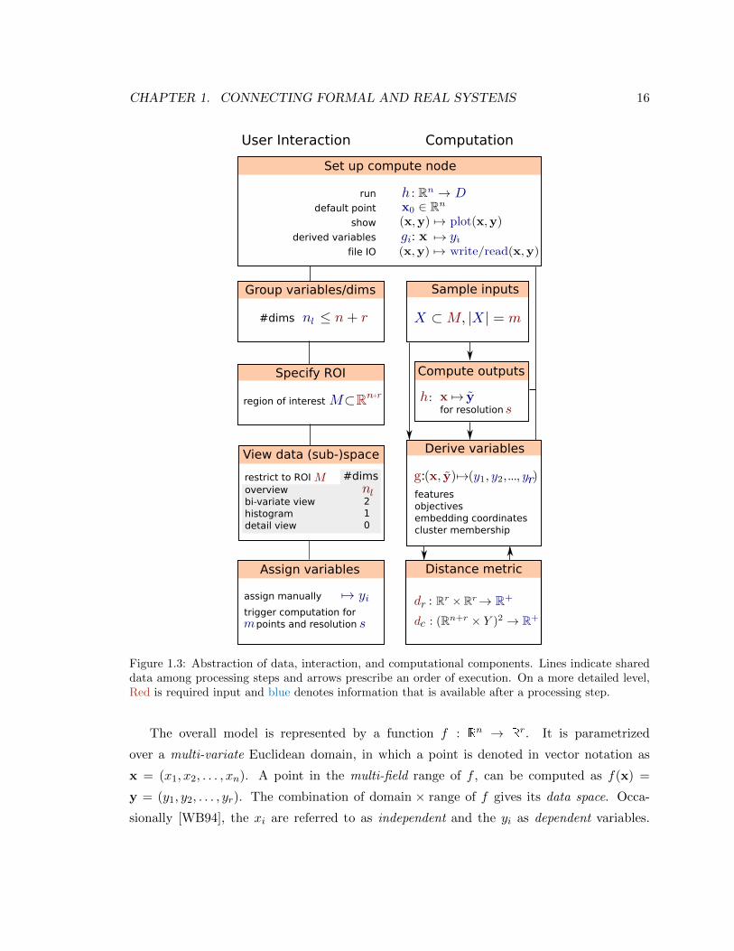
1.3 Abstraction of data, interaction, and computational components. Lines in-
dicate shared data among processing steps and arrows prescribe an order of
execution. On a more detailed level, Red is required input and blue denotes
information that is available after a processing step. . . . . . . . . . . . . . . 16
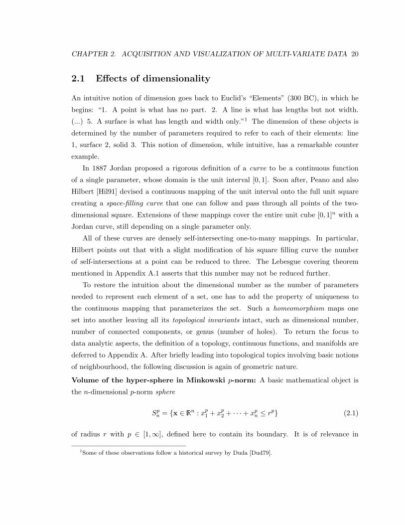
2.1 Semi-log plot of volumes of n = 1 . . . 30 – dimensional p-norm unit spheres. . 21
2.2 Set of 20 randomly distributed sample points in [0, 1]2 with Voronoi regions
outlined in blue and Voronoi relevant neighbours connected by grey lines.
Notice how the convex hull and the minimum spanning tree are part of the
grey Delaunay graph connecting Voronoi relevant neighbours. For points in
general position the Delaunay graph turns out to be a triangulation or a
simplicial complex in higher-dimensional spaces. . . . . . . . . . . . . . . . . 26
x
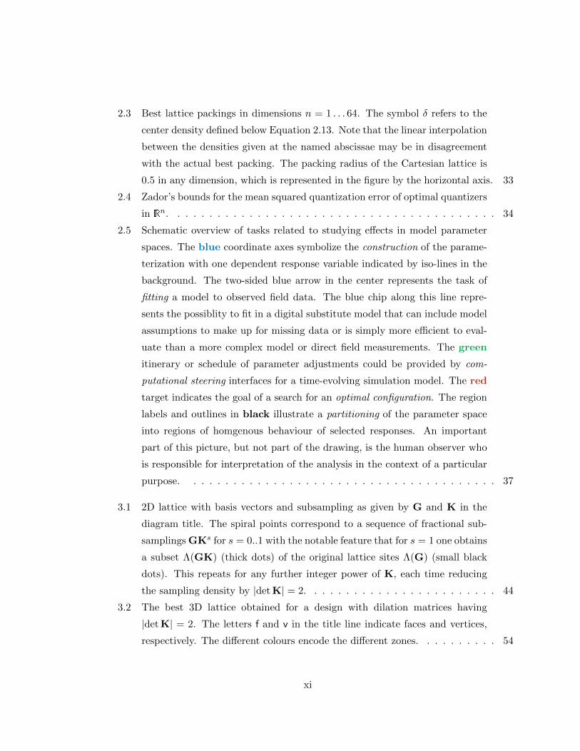
2.3 Best lattice packings in dimensions n = 1 . . . 64. The symbol δ refers to the
center density defined below Equation 2.13. Note that the linear interpolation
between the densities given at the named abscissae may be in disagreement
with the actual best packing. The packing radius of the Cartesian lattice is
0.5 in any dimension, which is represented in the figure by the horizontal axis. 33
2.4 Zador’s bounds for the mean squared quantization error of optimal quantizers
in Rn. . . . . . . . . . . . . . . . . . . . . . . . . . . . . . . . . . . . . . . . . 34
2.5 Schematic overview of tasks related to studying effects in model parameter
spaces. The blue coordinate axes symbolize the construction of the parame-
terization with one dependent response variable indicated by iso-lines in the
background. The two-sided blue arrow in the center represents the task of
fitting a model to observed field data. The blue chip along this line repre-
sents the possiblity to fit in a digital substitute model that can include model
assumptions to make up for missing data or is simply more efficient to eval-
uate than a more complex model or direct field measurements. The green
itinerary or schedule of parameter adjustments could be provided by com-
putational steering interfaces for a time-evolving simulation model. The red
target indicates the goal of a search for an optimal configuration. The region
labels and outlines in black illustrate a partitioning of the parameter space
into regions of homgenous behaviour of selected responses. An important
part of this picture, but not part of the drawing, is the human observer who
is responsible for interpretation of the analysis in the context of a particular
purpose. . . . . . . . . . . . . . . . . . . . . . . . . . . . . . . . . . . . . . . 37
3.1 2D lattice with basis vectors and subsampling as given by G and K in the
diagram title. The spiral points correspond to a sequence of fractional sub-
samplings GKs for s = 0..1 with the notable feature that for s = 1 one obtains
a subset Λ(GK) (thick dots) of the original lattice sites Λ(G) (small black
dots). This repeats for any further integer power of K, each time reducing
the sampling density by |det K| = 2. . . . . . . . . . . . . . . . . . . . . . . . 44
3.2 The best 3D lattice obtained for a design with dilation matrices having
|det K| = 2. The letters f and v in the title line indicate faces and vertices,
respectively. The different colours encode the different zones. . . . . . . . . . 54
xi

3.3 Three non-equivalent 2D lattices obtained for a design with dilation matrices
having |det K| = 2. The lattice in the first column is the known quincunx
sampling with a rotation of θ = 45. The other two are new schemes with
different rotation angles. The thick dots show the sample positions that are
retained after subsampling by K. The second row shows the same lattice at
twice the density, with more iteration levels of similarity transformed Voronoi
cells. . . . . . . . . . . . . . . . . . . . . . . . . . . . . . . . . . . . . . . . . . 55
3.4 Four non-equivalent 2D lattices obtained for a design with dilation matrices
having |det K| = 3. The lattice on the left is the well known hexagonal lattice
with a θ = 30 rotation. The other three are new schemes with different
rotation angles. . . . . . . . . . . . . . . . . . . . . . . . . . . . . . . . . . . . 55
3.5 Comparison of packing radii of best known packings, Cartesian packing, and
the upper bound as in Figure 2.3 on page 33. In addition, some designs of
this chapter are shown that enjoy the low-rate rotational reduction property
of Equation 3.2 for rates β ∈ 2, 3. If proceeding directly from a companion
K as provided by Algorithm 2 unoptimized constructions can be generated
instantly for any n. The optimized designs are obtained by maximization of
the packing radius over choices of S in Equation 3.9. The depicted results
beat Cartesian packing in all cases except for n ∈ 1, 3. . . . . . . . . . . . 56
4.1 Sampling comparison. The data y = f(x) (a) is composed with a transfer
function g(y) (b). Figures (c) and (d) show sinc-interpolated samplings of
g(f(x)). The tighter bounding frequency (d) suggested in this chapter re-
sults in 5 times fewer samples for these particular f and g, still truthfully
representing the composite signal. . . . . . . . . . . . . . . . . . . . . . . . . . 58
4.2 The frequency map K(ω, ν) for a function f(x) determines how much a fre-
quency ν of g contributes to a frequency ω of the spectrum of the composed
function g(f(x)). The examples are (a) single and (c) mixed non-normalized
Gaussians, using ϕ(µ, σ, x) = exp(−(x− µ)2/(2σ2)
)and their correspond-
ing K(ω, ν) in (b) and (d), respectively. The upper and lower slopes of the
low-valued cones (black) are given by the reciprocal of the maximum and the
minimum values of f ′, respectively, as shown in Section 4.1.2. . . . . . . . . . 61
xii
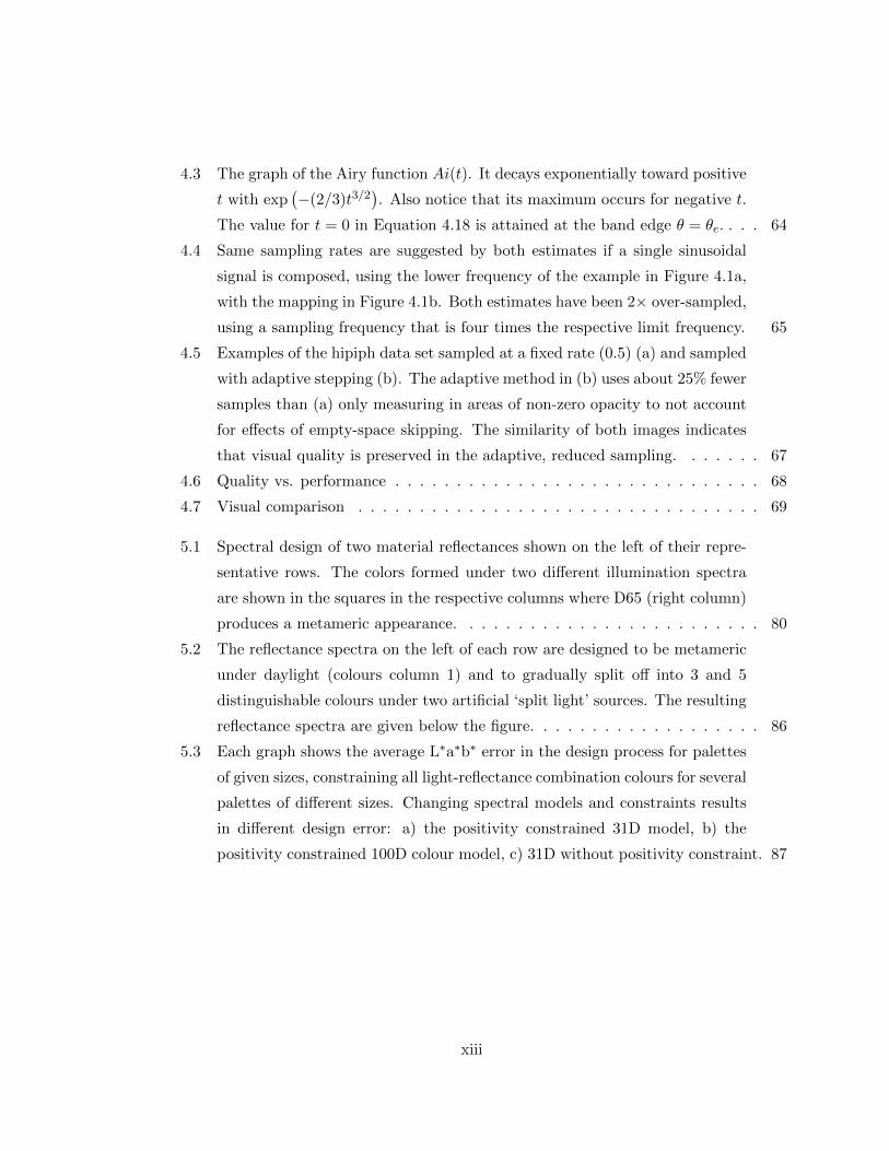
4.3 The graph of the Airy function Ai(t). It decays exponentially toward positive
t with exp(−(2/3)t3/2
). Also notice that its maximum occurs for negative t.
The value for t = 0 in Equation 4.18 is attained at the band edge θ = θe. . . . 64
4.4 Same sampling rates are suggested by both estimates if a single sinusoidal
signal is composed, using the lower frequency of the example in Figure 4.1a,
with the mapping in Figure 4.1b. Both estimates have been 2× over-sampled,
using a sampling frequency that is four times the respective limit frequency. 65
4.5 Examples of the hipiph data set sampled at a fixed rate (0.5) (a) and sampled
with adaptive stepping (b). The adaptive method in (b) uses about 25% fewer
samples than (a) only measuring in areas of non-zero opacity to not account
for effects of empty-space skipping. The similarity of both images indicates
that visual quality is preserved in the adaptive, reduced sampling. . . . . . . 67
4.6 Quality vs. performance . . . . . . . . . . . . . . . . . . . . . . . . . . . . . . 68
4.7 Visual comparison . . . . . . . . . . . . . . . . . . . . . . . . . . . . . . . . . 69
5.1 Spectral design of two material reflectances shown on the left of their repre-
sentative rows. The colors formed under two different illumination spectra
are shown in the squares in the respective columns where D65 (right column)
produces a metameric appearance. . . . . . . . . . . . . . . . . . . . . . . . . 80
5.2 The reflectance spectra on the left of each row are designed to be metameric
under daylight (colours column 1) and to gradually split off into 3 and 5
distinguishable colours under two artificial ‘split light’ sources. The resulting
reflectance spectra are given below the figure. . . . . . . . . . . . . . . . . . . 86
5.3 Each graph shows the average L∗a∗b∗ error in the design process for palettes
of given sizes, constraining all light-reflectance combination colours for several
palettes of different sizes. Changing spectral models and constraints results
in different design error: a) the positivity constrained 31D model, b) the
positivity constrained 100D colour model, c) 31D without positivity constraint. 87
xiii
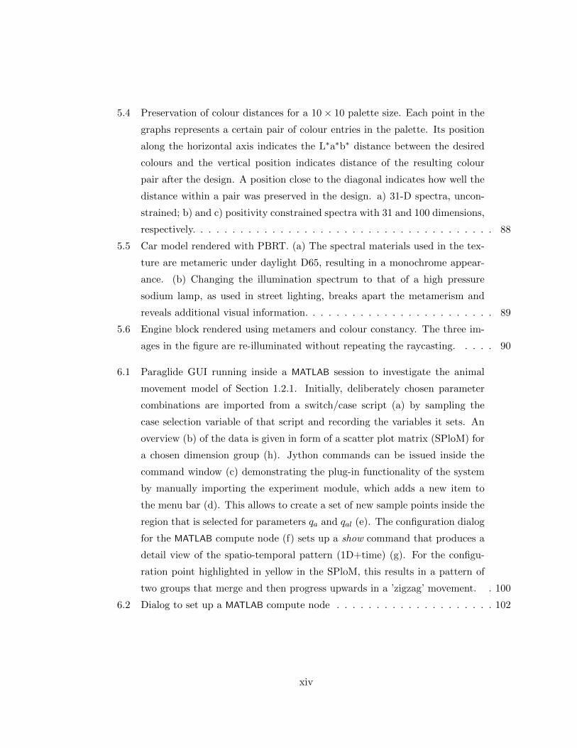
5.4 Preservation of colour distances for a 10× 10 palette size. Each point in the
graphs represents a certain pair of colour entries in the palette. Its position
along the horizontal axis indicates the L∗a∗b∗ distance between the desired
colours and the vertical position indicates distance of the resulting colour
pair after the design. A position close to the diagonal indicates how well the
distance within a pair was preserved in the design. a) 31-D spectra, uncon-
strained; b) and c) positivity constrained spectra with 31 and 100 dimensions,
respectively. . . . . . . . . . . . . . . . . . . . . . . . . . . . . . . . . . . . . . 88
5.5 Car model rendered with PBRT. (a) The spectral materials used in the tex-
ture are metameric under daylight D65, resulting in a monochrome appear-
ance. (b) Changing the illumination spectrum to that of a high pressure
sodium lamp, as used in street lighting, breaks apart the metamerism and
reveals additional visual information. . . . . . . . . . . . . . . . . . . . . . . . 89
5.6 Engine block rendered using metamers and colour constancy. The three im-
ages in the figure are re-illuminated without repeating the raycasting. . . . . 90
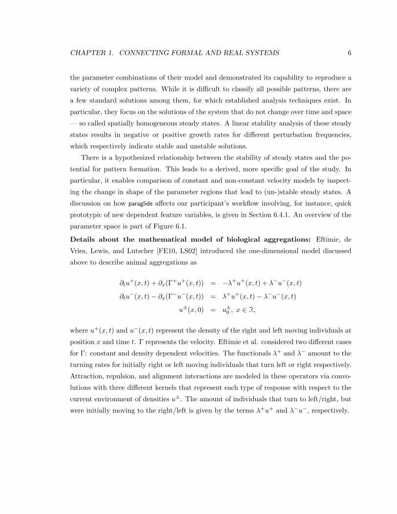
6.1 Paraglide GUI running inside a MATLAB session to investigate the animal
movement model of Section 1.2.1. Initially, deliberately chosen parameter
combinations are imported from a switch/case script (a) by sampling the
case selection variable of that script and recording the variables it sets. An
overview (b) of the data is given in form of a scatter plot matrix (SPloM) for
a chosen dimension group (h). Jython commands can be issued inside the
command window (c) demonstrating the plug-in functionality of the system
by manually importing the experiment module, which adds a new item to
the menu bar (d). This allows to create a set of new sample points inside the
region that is selected for parameters qa and qal (e). The configuration dialog
for the MATLAB compute node (f) sets up a show command that produces a
detail view of the spatio-temporal pattern (1D+time) (g). For the configu-
ration point highlighted in yellow in the SPloM, this results in a pattern of
two groups that merge and then progress upwards in a ’zigzag’ movement. . 100
6.2 Dialog to set up a MATLAB compute node . . . . . . . . . . . . . . . . . . . . 102
xiv
6.3 The light dial – interface to control the mixture of lights using normalized
inverse distances of the mixture selector (yellow circle) to the light nodes
(bulb icons) (see Eq. 6.1). . . . . . . . . . . . . . . . . . . . . . . . . . . . . . 109
6.4 (a) Graphical user interface (GUI) for the BCF2000 mixing board (b) showing
an experimental trial in progress. . . . . . . . . . . . . . . . . . . . . . . . . 112
6.5 Recorded slider motion paths for item 6: [ . . . . . . 110 110]+/-1 shown in
front of non-manipulation intervals (gray) and mistake intervals (red). The top row
is mixer interaction of a participant performing item ID 6 of forthcoming Figure 6.6
in three trial blocks for each of the two input methods in Figure 6.4. An error moving
irrelevant slider 6 is indicated in the third block. The path correlation matrix in the
right column is discussed in Section 6.3.2.1. . . . . . . . . . . . . . . . . . . . . . 113
6.6 Simultaneous manipulation of sliders as indicated by the maximum (in abso-
lute value) of the normalized slider-slider velocity cross-correlations of Equa-
tion 6.2. Simultaneity varies for different items and participants. . . . . . . . 115
6.7 Illustrating the sample creation in a sub-region of the parameter space it-
erating from coarse to finer sampling. (Un-)filled circles indicate parameter
configurations that lead to an (un-)stable steady state. . . . . . . . . . . . . 119
6.8 Scatter plot matrix view that compares the point embedding (lower left) with
the objective measures that went into computing its underlying similarity
measure. The numbering of the responses corresponds to the class labels of
Figure 1.1 (ID 5: cerebellum and 6: putamen). . . . . . . . . . . . . . . . . . 121
6.9 Scatter plot matrix view of the good cluster (yellow) identified in Figure 6.8
viewed in the subspace of input parameters. In this view sigma and alpha3
indicate clear thresholds beyond which the good configurations are found. . 122
6.10 Two layouts for 204 example experiments. a) input space showing variation
in current and input temperature, b) embedding of the same samples where
spatial proximity reflects plot similarity for cell current density, c) similarity
embedding for membrane electrode assembly (MEA) water content using the
same clusters as assigned in (b). Cluster representatives are shown in Fig-
ure 6.11 and Figure 6.12. These screenshots are from the 2007 C++ version
of paraglide, and are also attainable in the currently discussed Java implemen-
tation. . . . . . . . . . . . . . . . . . . . . . . . . . . . . . . . . . . . . . . . 124
6.11 Cell current density plots for the clusters in Figure 6.10b . . . . . . . . . . . 125
xv
6.12 MEA water content plots for the clusters labelled in Figure 6.10c . . . . . . 125
A.1 Illustration of the concept of forward cones F of Equation A.1 in a di-
rection u for the vertices of the white quadrangle, similar to Leydold and
Hormann [LH98, Fig. 3]. F (v1) begins in white, F (v2) and F (v3) in light
red and F (v4) in dark red. All cones extend infinitely towards the right, but
are artificially cut of in the picture. Even in practical computations this step
could be required to ensure that the valuations in Equation A.2 stay finite. . 135
B.1 (a) The sample density inside the unit cube jumps when scaling Cartesian
lattices in Rn for n = 2..4 using a scaled identity generating matrix R = αI.
(b) Discrepancy of various 3D point sets including some randomly rotated
regular lattices at differently scaled density. . . . . . . . . . . . . . . . . . . . 141
xvi
Chapter 1
Connecting formal and real systems
To record observations that are either made directly or are acquired with the aid of carefully
crafted devices is the starting point of the scientific method that prescribes how to construct
models that represent real-world systems. Here a system is understood as a collection of
things or concepts that exist by certain mechanisms or rules that in a formal system can
be laid out and verified rigorously. A model denotes a system that is intended to mimic
certain aspects of another system. A computational model is a formal system, where an
algorithm can be run for a given input configuration to compute an output description of the
simulated system. While such an algorithm is assumed to be deterministic, additional input
may introduce randomized behaviour. Having a model whose behaviour fits with available
observations, it becomes possible to diagnose or predict phenomena that occur at different
levels of structural organization, allowing to choose actions that influence development of
the system, or to utilize the observed effects in artificial constructions1 that, for instance,
improve quality of life.
Within this broad picture, the focus of this dissertation is to facillitate development,
analysis, and interpretation of computational models through efficient human interfaces.
This objective is approached at different stages of the modelling process through the lens of
parameter adjustment. Typical tasks and research challenges that arise when working with
computer model parameters are discussed in Section 2.4.1. The different approaches pursued
in the following chapters include a) methods for direct parameter choices, b) specification
of criteria that characterize good choices, and c) theoretical study of model properties that
1Note that the meaning of artificial as in human-made is a special case of natural.
1

CHAPTER 1. CONNECTING FORMAL AND REAL SYSTEMS 2
guide general parameter choice. The work of Chapter 6 enables manipulation of control
parameters in an interactive manner (a). A less direct path is taken in the computer
graphics setting of Chapter 5, where the user specifies criteria (b), such that globally optimal
parameter choices can be made automatically. Pursuing the adjustment of internal model
parameters, Chapter 4 performs a theoretical study (c) of properties of a fundamental data
processing step and uses the findings to determine a volume rendering parameter. On a
similarly theoretical level, Chapter 3 uses general criteria of uniformity in the design of a
space-filling sampling pattern where user input is merely required in form of a constraining
region and a budget for the number of sample points.
The underlying theme of human guidance is somewhat contrary to typical objectives of
algorithm development that seek to eliminate the need for human input as much as possible
in order to obtain consistent results efficiently. When asking someone on the hallway of the
computing science department how this is supposed to be done, the typical answers boil down
to: “Think harder about the problem, incorporate into your algorithm what is known and
improve the theory where it is insufficient.” While it is imaginable to eventually automate
information collection [PBMW99] and inference mechanisms [BWB09], thinking about a
problem in its original domain and improving a model abstraction of it are still very much
human-centric tasks. Also, when a ready-made model is employed that influences choices
that affect people, e.g., regarding the health of a human being, the livability of a city in
planning, or if it informs decisions regarding the economy of a country or our environment
— why would we want to give up the ability a) to convince ourselves that the model does
the right thing (is valid); b) to give hints that make up for missing information from our
experience, knowledge, or intuition; or c) to make human inventiveness available to get a
better2 model more quickly?
The specific examples that I will give in Section 1.2 are a bit smaller scale than what
was just mentioned. However, these computational modelling settings also share a need for
human input. This need provides a basic motivation for visualization3 as a discipline at
the core of scientific study. The particular focus on visual methods to map properties of
data to the screen is justified due to our well developed visual perception. The simultaneity
2Better here means a model with a strong linkage to the real-world system that it is intended to repre-sent. [SRA+08, Ch. 1]
3Beyond the technical scope, the term visualization is also understood as a method of thinking, learn-ing, and communication that works with mental imagery and its transformation, e.g., to improve athleticperformance [GC08]. However, in our research context the meaning is confined to the computational domain.
CHAPTER 1. CONNECTING FORMAL AND REAL SYSTEMS 3
and spatial resolution of visual processing are unparalleled by other senses, such as touch
or hearing [Gol10, pp. 888]. It enables us to integrate a massive stream of cues for location,
shape, motion, colour, or textural properties that are presented by a still image or an ani-
mated sequence. Visualization research seeks to utilize this natural processing apparatus by
devising effective visual encodings and interaction metaphors that work with data [Mun12].
However, the quality of any data display hinges on the relevance of the given data for
the driving questions. Hence, in extension of the classical scope of visualization research,
my dissertation is looking at user involvement in the acquisition of data. Specifically, this
concerns sampling of continuous phenomena, as well as adjustments in parameter spaces of
computational models.
1.1 Contributions of this dissertation
The remainder of this first chapter will perform a characterization of several domains of
computer experimentation to derive a set of requirements for human-guided study of models
in Section 1.3. Building on this analysis towards the end of this thesis, Chapter 6 then
proposes paraglide — a framework for user-driven analysis of parameter effects. Its main
point is to facilitate a workflow that results in a partitioning of the continuous space of
model configurations into regions of distinct system behaviour.
Establishing a model often involves the adjustment of multiple parameters. The contri-
bution of the theoretical survey4 in Chapter 2 is to show effects that arise when discretizing
multi-dimensional Euclidean space with a minimal budget of points. This also prepares the
background for the remaining chapters.
One feature of paraglide is to elevate user interaction from specifying point locations in
parameter searches to a higher level of outlining constraints of a region that can then be
filled with a given budget of points (see Section 6.2.3). To be able to fill this space efficiently
is the motivation behind Chapter 3, where a class of point sets is designed to directly fulfill
a number of quality criteria. To facilitate progressive regional exploration, point lattices
are constructed that contain rotated and scaled versions of themselves. Their distinguishing
property is that different levels of resolution share a single type of Voronoi polytope, whose
volume grows independently of the dimensionality by a chosen integer factor as low as 2.
4The human interface in this context are systematic methods of thinking provided by mathematics.
CHAPTER 1. CONNECTING FORMAL AND REAL SYSTEMS 4
Many real world phenomena can be viewed in 3-dimensional Euclidean space together
with a time coordinate. Hence, a common type of data in numerical visualization are
grids that represent some physical quantity for each point in a bounded volume. In order to
reduce sampling costs while maintaining image quality when rendering such data, Chapter 4
presents a Fourier domain analysis of the effect of composing a data signal with a function
that assigns visibility to relevant values. Based on this, a previous lower bound for a sufficient
sampling frequency is relaxed and applied to adaptively choose the step size in raycasting.
Using a spectral light model, it is possible to improve physical realism and to create
colour effects that scale the level of distinguishable detail in a visualization. To help mod-
ellers to make useful decisions in a high-dimensional design space of palettes of lights and
materials, Chapter 5 devises a method that generates a palette of presets that optimally
fulfill a set of design criteria. A brief excursion in Section 6.3 discusses two alternative user
interfaces for steering a multi-dimensional cursor that can also be applied to unobtrusively
search for a suitable mixture.
A word on the narrator’s perspective: While I take care to not claim contributions
in this thesis that are not mine, I recognize that ideas are not born in a vacuum and will
therefore in the following adapt the pronoun we to refer to me as a researcher, the group I
was working with, or to engage the readership, which should be clear from context. I will
explicitly state external contributions where sources are otherwise not clear.
1.2 Problem domains that require parameter tuning
In order to get a more detailed understanding of needs and requirements for user-driven
parameter space navigation, we engaged in a problem characterization phase by conducting
contextual interviews with six experts from three different domains: engineering, mathe-
matical modelling, and segmentation algorithm development. Based on that, we summarize
design requirements in Section 1.3 that are more general yet grounded in real-world appli-
cation areas.
Our methodology corresponds to Munzner’s nested model [Mun09], which casts good
practices of software engineering into the realm of visualization research validation. With
this background, we prepare the discussion of effective visual encodings and interaction
techniques in Chapter 6, where our tool paraglide is presented and validated. This motivates
the remaining chapters that discuss efficient algorithms for related purposes.
CHAPTER 1. CONNECTING FORMAL AND REAL SYSTEMS 5
1.2.1 Mathematical modelling: Collective behaviour in biological aggre-
gations
Our first target group are two researchers studying properties of a mathematical model that
describes spatial and spatio-temporal patterns of biological aggregations. Furthering the
understanding of such patterns helps to predict animal migration behaviour, e.g., to better
understand how, where, and when fish aggregations form to suggest more efficient fishing
strategies [Par99]. Modelled patterns can also inform measures to contain plagues of locusts
and positively affect quality of life in developing countries [BSC+06].
To study those spatio-temporal patterns, our participants developed a mathematical
model [FE10, LS02] consisting of a system of partial differential equations (PDEs) that
express in one spatial dimension how left and right travelling densities of individuals move
and turn over time, with details provided at the end of this section. The basic idea is to
take three kinds of social forces into account — namely attraction, repulsion, and alignment
— that act globally among the densities of individuals. Attraction is the tendency between
distant individuals to get closer to each other, repulsion is the social force that causes indi-
viduals in close proximity to repel from each other, and alignment represents the tendency
to sync the direction of motion with neighbours. Solving the model for different choices of
coefficients produces many complex spatial and spatio-temporal patterns observed in na-
ture, such as stationary aggregations formed by resting animals, zigzagging flocks of birds,
milling schools of fish, and rippling behaviour observed in Myxobacteria.
Our use case is part of a Master’s thesis on this subject with a focus on comparing two
versions of their model [Abd11]. In the first one the velocity is constant. In the second
one the individuals speed up or slow down as a response to their social interactions with
neighbours. Comparing these models requires to solve them numerically for several different
configurations. Each instance of the model corresponds to one specific choice of the 14 model
parameters that include the coefficients for the three postulated social forces. The output
of the simulation is a spatio-temporal pattern of population densities. The number of basis
functions is an internal parameter that gives the resolution in space and time and influences
the trade-off for accuracy vs. runtime, which for reasonable output lies between 2 minutes
and half an hour. With 5 minutes each, one can perform a full computation of close to 300
sample points in the duration of a single day.
To better understand the space of possible solutions, our participants manually explored
CHAPTER 1. CONNECTING FORMAL AND REAL SYSTEMS 6
the parameter combinations of their model and demonstrated its capability to reproduce a
variety of complex patterns. While it is difficult to classify all possible patterns, there are
a few standard solutions among them, for which established analysis techniques exist. In
particular, they focus on the solutions of the system that do not change over time and space
— so called spatially homogeneous steady states. A linear stability analysis of these steady
states results in negative or positive growth rates for different perturbation frequencies,
which respectively indicate stable and unstable solutions.
There is a hypothesized relationship between the stability of steady states and the po-
tential for pattern formation. This leads to a derived, more specific goal of the study. In
particular, it enables comparison of constant and non-constant velocity models by inspect-
ing the change in shape of the parameter regions that lead to (un-)stable steady states. A
discussion on how paraglide affects our participant’s workflow involving, for instance, quick
prototypic of new dependent feature variables, is given in Section 6.4.1. An overview of the
parameter space is part of Figure 6.1.
Details about the mathematical model of biological aggregations: Eftimie, de
Vries, Lewis, and Lutscher [FE10, LS02] introduced the one-dimensional model discussed
above to describe animal aggregations as
∂tu+(x, t) + ∂x(Γ+u+(x, t)) = −λ+u+(x, t) + λ−u−(x, t)
∂tu−(x, t)− ∂x(Γ−u−(x, t)) = λ+u+(x, t)− λ−u−(x, t)
u±(x, 0) = u±0 , x ∈ R,
where u+(x, t) and u−(x, t) represent the density of the right and left moving individuals at
position x and time t. Γ represents the velocity. Eftimie et al. considered two different cases
for Γ: constant and density dependent velocities. The functionals λ+ and λ− amount to the
turning rates for initially right or left moving individuals that turn left or right respectively.
Attraction, repulsion, and alignment interactions are modeled in these operators via convo-
lutions with three different kernels that represent each type of response with respect to the
current environment of densities u±. The amount of individuals that turn to left/right, but
were initially moving to the right/left is given by the terms λ+u+ and λ−u−, respectively.
CHAPTER 1. CONNECTING FORMAL AND REAL SYSTEMS 7
1.2.2 Bio-medical imaging: Segmentation algorithm
Saad et al. [SHMS08] use a kinetic model to devise a multi-class, seed-initialized, iterative
segmentation algorithm for molecular image quantification. Due to the low signal-to-noise
ratio and partial volume effect present in dynamic-positron emission tomography (d-PET)
data, their segmentation method has to incorporate prior knowledge. In this noisy setting,
the segmentation of a basic random walker [Gra06] would just result in Voronoi regions
around the seed points. An extension by Saad et al. makes this method usable for noisy
data by adding energy terms that account for desirable criteria, such as data fidelity, shape
prior, intensity prior, and regularization.
In order to attain the superior segmentation quality of the algorithm, a proper choice
of weights for the energy mixture is crucial. To facilitate this choice of weight parameters,
their code provides numerical performance measures that assess the quality of each segment.
One such measure is the Dice coefficient [Dic45], which gives a ratio of overlap with labelled
training data. A second measure expresses an error of the quality of the kinetic modelling.
Overall, the algorithm is influenced by eight factors (parameters). Ten response variables
provide two quality measures per segment, disregarding background.
The model calibration could proceed by numerical optimization of the performance.
However, for that a choice of importance weights has to be given, which again is a step where
in the general setting human input is required. However, for instance the Dice coefficients
that indicate agreement of the segmented shape with given training data for putamen,
using the two configurations of Figure 1.1(c) and (d), are both above the 90th percentile
of the sampled configurations and less than 0.003 standard deviations apart. Numerically,
this means that both segmentations are of the same, near optimal quality. Yet by visual
inspection, it is possible to tell that the putamen (PN) shape in (d) is favourable over the
one obtained in (c). Hence, guidance of a domain expert is desirable to sort among several
candidate solutions in order to find an improved segmentation, which is hard or impossible
to choose automatically. A workflow for such a procedure is subject of Section 6.4.2.
1.2.3 Engineering: Fuel cells
A fuel cell takes hydrogen and oxygen as gaseous input and converts them into water and
heat, while generating an electric current. Affordable, high-performance fuel cells have the
CHAPTER 1. CONNECTING FORMAL AND REAL SYSTEMS 8
(a) raw data (b) ground truth
(c) config# 13, dice6 = .8136 (d) config# 44, dice6 = .8128
Figure 1.1: Classification of a slice of d-PET data using two different parameter configurations.The classes are 1: background (BG), 2: skull (SK), 3: grey matter (GM), 4: white matter (WM), 5:cerebellum (CM), and 6: putamen (PN).
potential to enable more environmentally friendly means of transport without any CO2 emis-
sion. To manufacture a prototypical cell stack costs tens of thousands of dollars. Hence, a
reliable synthetic model can greatly bring down the price of finding an optimal configuration
for production.
The example investigated here is a simulation of a fuel cell stack developed by Chang
et al. [CKPW07]. Their stack model is a system of coupled one-dimensional PDEs de-
scribing the individual cells in the stack. It can be adjusted with about 100 parameters,
where suitable choices of values are known for most of these parameters from fitting to
available measurements. Computing a simulation run outputs 43 different plots that show
how certain physical quantities, such as current density, temperature, or relative humidity
vary across the geometry of the cell stack. The computer model can be rerun for differ-
ent configurations and, thus, allows for much broader exploration of design options than
real prototyping. In particular, engineers are interested in studying failure mechanisms
and to optimize performance under varying conditions for different groups of parameters

CHAPTER 1. CONNECTING FORMAL AND REAL SYSTEMS 9
that represent the geometry of the assembly (size and number of cells in a stack), material
properties (permeability), or running conditions (temperature, pressure, concentration for
cathode and anode). Experiments demonstrating the use of the suggested interactions are
given in Section 6.4.3.
1.2.4 Visualization: Scene setup and rendering algorithm configuration
The following two use cases are located in a research laboratory, which is a natural envi-
ronment for model development. A topic of particular interest at the Graphics, Usability,
and Visualization (GrUVi)-Lab at Simon Fraser University is to improve techniques for the
visualization of volumetric data. This kind of data can capture physical quantities, such
as density, flow, or tensor information in a bounded spatial domain and is used to answer
diagnostic and predictive questions in fields as diverse as health care, environmental studies,
or engineering. In both cases, I was part of the group, but the objectives and developed
tool chain apply to different follow-up projects, beyond the initial one described here.
1.2.4.1 Rendering algorithm parameters
The goal of this project in 2005 was to make headway into the open problem of providing
guidelines to choose optimal configuration parameters of a volume rendering algorithm.
Ideally, this should lead to informative views of the studied data that are of sufficient
quality, do not miss any important features, and that can be computed at minimal cost.
While the previous cases where suggesting interactive experimentation, such a proce-
dure amounted to current practices in this particular use case that is described in the
following. To facillitate a pilot study that would allow first statements about the rendering
problem, I developed an object oriented implementation of a raycaster based on C++ tem-
plate mechanisms and integrated it into the lab software vuVolume, which is published on
sourceforge.net.
The customizable raycaster could be interacted with at runtime by writing and read-
ing a hierarchical XML description of its state. This way, computation for many different
configurations could be done offline with bash scripted for-loops that would combine pre-
set XML snippets to set data, transfer function, lighting model, camera, and reconstruction
parameters [MMMY97]. Different configurations influence the resulting image quality and
processing costs for time and memory. For each setup we generated one image with a
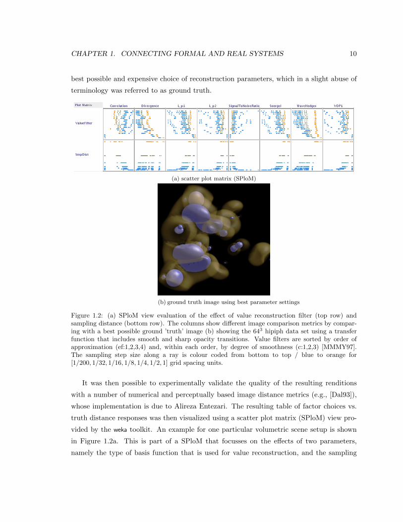
CHAPTER 1. CONNECTING FORMAL AND REAL SYSTEMS 10
best possible and expensive choice of reconstruction parameters, which in a slight abuse of
terminology was referred to as ground truth.
(a) scatter plot matrix (SPloM)
(b) ground truth image using best parameter settings
Figure 1.2: (a) SPloM view evaluation of the effect of value reconstruction filter (top row) andsampling distance (bottom row). The columns show different image comparison metrics by compar-ing with a best possible ground ’truth’ image (b) showing the 643 hipiph data set using a transferfunction that includes smooth and sharp opacity transitions. Value filters are sorted by order ofapproximation (ef:1,2,3,4) and, within each order, by degree of smoothness (c:1,2,3) [MMMY97].The sampling step size along a ray is colour coded from bottom to top / blue to orange for[1/200, 1/32, 1/16, 1/8, 1/4, 1/2, 1] grid spacing units.
It was then possible to experimentally validate the quality of the resulting renditions
with a number of numerical and perceptually based image distance metrics (e.g., [Dal93]),
whose implementation is due to Alireza Entezari. The resulting table of factor choices vs.
truth distance responses was then visualized using a scatter plot matrix (SPloM) view pro-
vided by the weka toolkit. An example for one particular volumetric scene setup is shown
in Figure 1.2a. This is part of a SPloM that focusses on the effects of two parameters,
namely the type of basis function that is used for value reconstruction, and the sampling

CHAPTER 1. CONNECTING FORMAL AND REAL SYSTEMS 11
distance that is used when numerically accumulating radiance along rays through the re-
constructed volume. When combined for all wavelengths this gives the colour information
that is displayed in each pixel of the rendered image as shown in Figure 1.2b.
While these graphs do not lend themselves to derive concise, generalizable statements
about the rendering problem, they do show significant effects of sampling distance, and of
the order of approximation of the reconstruction basis. This pilot study also showed that a
satisfactory exploration of all rendering parameter effects using nested for-loops is infeasible.
1.2.4.2 Scene parameters
In order to render a scene it has to be constructed first. As will be explained in Section 5.1,
modelling techniques for geometry have already received much attention in graphics re-
search, whereas the construction of synthetic materials still has important open questions
to offer.
An aspect of particular interest in our lab, was the support of more complete light models
considering full spectral power distributions (SPDs) instead of tri-chromatic (red,green,blue)-
tuples In our previous work [BMDF02], we outlined the usefulness of a more complete light-
ing model, by pointing out that it enables two complementary directions: improved physical
realism, as well as increased design freedom for artificial effects.
Materials and light sources: In order to find SPDs to configure light sources and mate-
rials in a scene, one can either acquire them using a measurement device, obtain data bases
of spectra from the web, or construct new ones by mixing combinations of a smaller set.
Note that the inclusion of lights in this construction is already a step beyond classical
computer graphics, where one simply sets up (red, green, blue)-triples for each surface
point and illuminates with a white light. Designers of a scene that care about correct
colour reproduction when illuminating with something else than just white light need to
find spectra that produce specific colours for particular combinations of illuminant and
surface. Alternatively, one could also ask for perceived colour differences between certain
materials to be zero. The task of a designer who constructs a scene is to come up with these
criteria and to find materials that fulfill them.
Considering the huge size of the design space in relation to the small size of desirable
solutions, this is a very difficult, if not infeasible adjustment problem. This poses a research
problem that is addressed in Chapter 5, where also the lack of current practices for this
CHAPTER 1. CONNECTING FORMAL AND REAL SYSTEMS 12
purpose and directions for improvement are elaborated further.
Light mixtures: In the scenes we consider the superposition principle of light applies. So,
given a designed palette with light sources, a remaining task is to define a linear mixture
of these lights or a transition of mixtures that produce a convincing visualization. For
a complete setup one would adjust the geometry of the lights and move them around to
achieve the desired effects. More abstractly, this amounts to choosing a vector of weights
that results in a set of desired colours for all surfaces in view. Due to the central role
of human judgement in this setting, this poses an interactive adjustment task for which
Section 6.3 investigates two different practical solutions.
1.3 Task structure
All previous use cases are motivated by questions about a real-world system. In each
setting, domain knowledge about the problem has been expressed in form of a computational
model and the parameter space of the model is explored in order to relate observations
about its properties to the corresponding real setting. Please refer to the previous
subsections for details about the parameter spaces in the respective settings. The studies
share a set of requirements as summarized in Table 1.1.
Table 1.1: Summary of the requirement analysis.
R1: integrate with existing practices and code
R2: specify parameter region of interest (ROI)
R2a: sample ROI and compute data set
R3: browse data providing overview (R3a) and detail (R3b)
R4: construct feature variables (manually labelled or computed)
R4a: combine features to derive a distance metric
R5: identify region(s) of similar outcome in parameter space
R6: find optimal point for a particular dependent variable or user notion
R7: analyse sensitivity of feature values to change in input
R8: save state of the project for later reproduction
R9: perform theoretical study that derives knowledge to improve the model
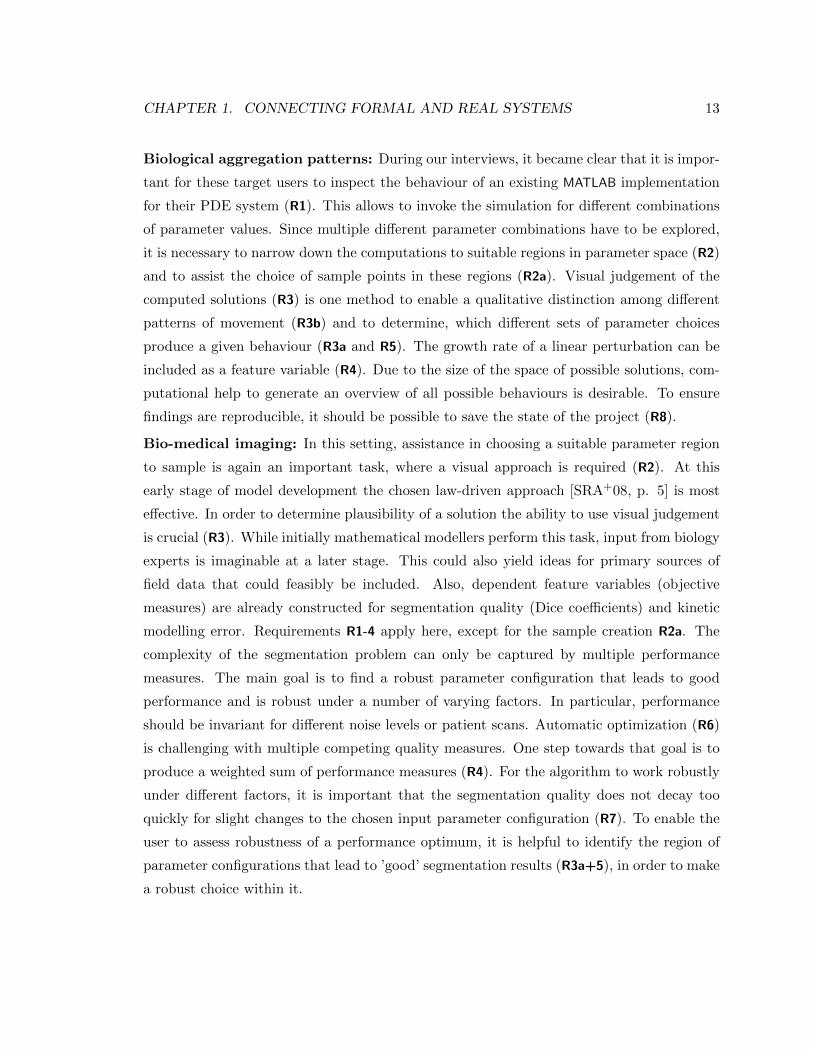
CHAPTER 1. CONNECTING FORMAL AND REAL SYSTEMS 13
Biological aggregation patterns: During our interviews, it became clear that it is impor-
tant for these target users to inspect the behaviour of an existing MATLAB implementation
for their PDE system (R1). This allows to invoke the simulation for different combinations
of parameter values. Since multiple different parameter combinations have to be explored,
it is necessary to narrow down the computations to suitable regions in parameter space (R2)
and to assist the choice of sample points in these regions (R2a). Visual judgement of the
computed solutions (R3) is one method to enable a qualitative distinction among different
patterns of movement (R3b) and to determine, which different sets of parameter choices
produce a given behaviour (R3a and R5). The growth rate of a linear perturbation can be
included as a feature variable (R4). Due to the size of the space of possible solutions, com-
putational help to generate an overview of all possible behaviours is desirable. To ensure
findings are reproducible, it should be possible to save the state of the project (R8).
Bio-medical imaging: In this setting, assistance in choosing a suitable parameter region
to sample is again an important task, where a visual approach is required (R2). At this
early stage of model development the chosen law-driven approach [SRA+08, p. 5] is most
effective. In order to determine plausibility of a solution the ability to use visual judgement
is crucial (R3). While initially mathematical modellers perform this task, input from biology
experts is imaginable at a later stage. This could also yield ideas for primary sources of
field data that could feasibly be included. Also, dependent feature variables (objective
measures) are already constructed for segmentation quality (Dice coefficients) and kinetic
modelling error. Requirements R1-4 apply here, except for the sample creation R2a. The
complexity of the segmentation problem can only be captured by multiple performance
measures. The main goal is to find a robust parameter configuration that leads to good
performance and is robust under a number of varying factors. In particular, performance
should be invariant for different noise levels or patient scans. Automatic optimization (R6)
is challenging with multiple competing quality measures. One step towards that goal is to
produce a weighted sum of performance measures (R4). For the algorithm to work robustly
under different factors, it is important that the segmentation quality does not decay too
quickly for slight changes to the chosen input parameter configuration (R7). To enable the
user to assess robustness of a performance optimum, it is helpful to identify the region of
parameter configurations that lead to ’good’ segmentation results (R3a+5), in order to make
a robust choice within it.
CHAPTER 1. CONNECTING FORMAL AND REAL SYSTEMS 14
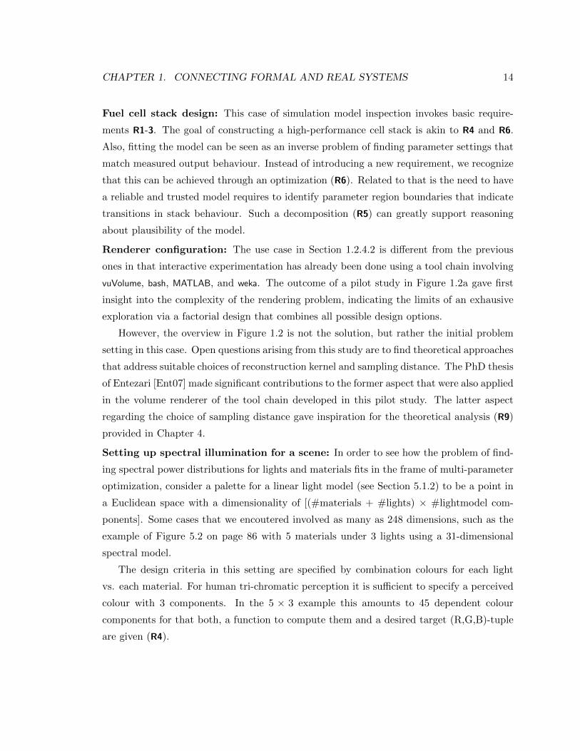
Fuel cell stack design: This case of simulation model inspection invokes basic require-
ments R1-3. The goal of constructing a high-performance cell stack is akin to R4 and R6.
Also, fitting the model can be seen as an inverse problem of finding parameter settings that
match measured output behaviour. Instead of introducing a new requirement, we recognize
that this can be achieved through an optimization (R6). Related to that is the need to have
a reliable and trusted model requires to identify parameter region boundaries that indicate
transitions in stack behaviour. Such a decomposition (R5) can greatly support reasoning
about plausibility of the model.
Renderer configuration: The use case in Section 1.2.4.2 is different from the previous
ones in that interactive experimentation has already been done using a tool chain involving
vuVolume, bash, MATLAB, and weka. The outcome of a pilot study in Figure 1.2a gave first
insight into the complexity of the rendering problem, indicating the limits of an exhausive
exploration via a factorial design that combines all possible design options.
However, the overview in Figure 1.2 is not the solution, but rather the initial problem
setting in this case. Open questions arising from this study are to find theoretical approaches
that address suitable choices of reconstruction kernel and sampling distance. The PhD thesis
of Entezari [Ent07] made significant contributions to the former aspect that were also applied
in the volume renderer of the tool chain developed in this pilot study. The latter aspect
regarding the choice of sampling distance gave inspiration for the theoretical analysis (R9)
provided in Chapter 4.
Setting up spectral illumination for a scene: In order to see how the problem of find-
ing spectral power distributions for lights and materials fits in the frame of multi-parameter
optimization, consider a palette for a linear light model (see Section 5.1.2) to be a point in
a Euclidean space with a dimensionality of [(#materials + #lights) × #lightmodel com-
ponents]. Some cases that we encoutered involved as many as 248 dimensions, such as the
example of Figure 5.2 on page 86 with 5 materials under 3 lights using a 31-dimensional
spectral model.
The design criteria in this setting are specified by combination colours for each light
vs. each material. For human tri-chromatic perception it is sufficient to specify a perceived
colour with 3 components. In the 5 × 3 example this amounts to 45 dependent colour
components for that both, a function to compute them and a desired target (R,G,B)-tuple
are given (R4).

CHAPTER 1. CONNECTING FORMAL AND REAL SYSTEMS 15
The task of finding suitable spectra in this setting is an inverse problem where one has to
choose factors (light and material SPDs) that produce given combination colour responses.
Rather than defining a new requirement item, this can be framed as an optimization prob-
lem (R6), for which manual search through this space is virtually impossible and, hence,
automatic assistance would be desirable. Rather than analysing sensitivity (R7) in this
case it actually needs to be controlled by introducing regularization terms that are decribed
further in Section 5.2.
Some of the spectra may be required to match real-world measurements and all of them
should be positive in order to be physically plausible, restricting the search to the positive
orthant. Constraining the solutions in this way can be seen as non-interactive construction
of a feasibility region (R2).
1.4 Data abstraction
A common theme of our use cases is that, unlike classical data visualization settings, they
do not start from given data, but work with a computational model, whose parameter space
is sampled in order to construct a set of data points for interactive analysis. Here, the
notion of a data source, which was recently introduced as abstraction of a file loader by
Ingram et al. [IMI+10], could be extended to include basic information about the available
variables, their types, and valid ranges. Enhanced with a capability to query new points
that are not yet stored in a data table, this could be used as an interface to static data
as well as dynamic computation, similar to a function call in a procedural programming
language. This results in a synthetic data source, which we refer to as compute node. The
design of a basic user interface for this abstraction will be discussed in Section 6.2.1. The
conceptual organization of the required tasks along with their inputs and outputs is shown
in Figure 1.3. It separately considers user interaction and computational pipeline, where all
modules operate on the same data and share one flow of control.
A numerical model in our cases consists of relations among a set of variables or dimen-
sions. Some background on relevant mathematical concepts is summarized in Appendix A.
Variables may be inherent to the problem domain or internal to the model. Further possible
distinction can be made considering the distribution of their values, which can be contin-
uous or discrete, (un-)known, (un-)observable, (in-)expensive to sample from, determined
empirically from data, or structurally inferred.
CHAPTER 1. CONNECTING FORMAL AND REAL SYSTEMS 16
Set up compute node
run
default point
show
derived variables
file IO
Group variables/dims
Specify ROI
View data (sub-)space
overviewbi-variate viewhistogramdetail view
Assign variables
assign manually
trigger computation for points and resolution
Sample inputs
Derive variables
Compute outputs
User Interaction Computation
Distance metric
featuresobjectivesembedding coordinatescluster membership
#dims
region of interest
restrict to ROI
#dims
210
for resolution
Figure 1.3: Abstraction of data, interaction, and computational components. Lines indicate shareddata among processing steps and arrows prescribe an order of execution. On a more detailed level,Red is required input and blue denotes information that is available after a processing step.
The overall model is represented by a function f : Rn → Rr. It is parametrized
over a multi-variate Euclidean domain, in which a point is denoted in vector notation as
x = (x1, x2, . . . , xn). A point in the multi-field range of f , can be computed as f(x) =
y = (y1, y2, . . . , yr). The combination of domain × range of f gives its data space. Occa-
sionally [WB94], the xi are referred to as independent and the yi as dependent variables.
CHAPTER 1. CONNECTING FORMAL AND REAL SYSTEMS 17
However, this notion does not apply in general, since the presence of constraints may intro-
duce dependencies among the xi. Alternative terminology for inputs and outputs of f are
factors and responses, or parameters and derived variables, respectively5.
We assume that code to compute f is given as a black box and can be invoked for a set
of points X = xk ⊂ Rn of finite size m = |X|. This set X is referred to as a design or a
sample [SWN03, p. 15]. With a prescribed ordering this amounts to the construction of a
design matrix X ∈ Rm×n containing the points in its m rows (R2a). The mapping f gives a
set of responses Y = f(xk). By concatenating these values as [X Y] ∈ Rm×(n+r) the data
table is obtained, giving the main input to further processing or visualization. Applying the
concept of a function f , we impose that the output of the code is deterministic. Uncertainties
of the system can still be modelled by specifying probability distributions for additional
environmental variables xi [SWN03, p. 121]. Even for non-deterministic code, such an
additional variable could simply index the order or the time of a particular invocation.
Using the conceptual ingredients of Figure 1.3, f is formed by composing a potentially
costly image computation h (R1) and variable derivation g (R4) to give f = g h. The
image of h is meant in a mathematical sense, but can represent an actual picture or a disk
image that captures the result of the computation for a particular configuration x. This
indirection should emphasize the possibility to cache output images y ∈ D, but in simple
cases the derived response variables yi are computed directly and g is just the identity
D = Rr → Rr.
Depending on what derived variable yi = gi(y) is specified (R4), its information may be
interpreted as a feature, embedding coordinate, cluster membership label, likelihood, dis-
tance from a template point, or objective measure (R6) — to give a few practical examples.
In each case it may be possible to compute gi or to assign values manually, depending on
whether a function definition or a user’s concept is available.
Some processing steps (R5+7) require a notion of distance or similarity among points
(R4a). Technical background on distances and norms is provided in Appendix A.1.1.
One method considered here is the Euclidean distance dr between feature vectors in Rr.
Beyond that, distance dc combines all information about each configuration point, including
its parameter coordinates x ∈ Rn or a domain specific function operating on the disk images.
In order to accommodate simulations with a large number of variables n + r, an early
5This is a summary of terminology found in the referenced data analysis literature.

CHAPTER 1. CONNECTING FORMAL AND REAL SYSTEMS 18
step of the interaction allows the user to divide variables into groups of smaller sizes nl.
This way one can separate input and output, indicate other semantic information inherent
to the simulation model, and produce more focussed multi-variable views (R3).
An important aspect of Figure 1.3 is that the sample creation is split into a specification
of a region of interest M ⊂ Rn+r, where areas in the input space are outlined (R2), see also
Section 6.2.3. This is input to an automatic method that generates a point distribution of
good numerical quality in that region that also fulfills a given budget m. What good quality
means in the context of multi-dimensional point distribution is subject of the following
chapter.
Chapter 2
Acquisition and visualization of
multi-variate data
Enabling people to inspect and understand complex data sets is a core objective of computa-
tional visualization. While algorithms may apply to general data types, staying aware of the
original problem domain is crucial to allow for meaningful interpretation of a visualization.
Aside from this cognitive motivation there are also computational reasons to maintain the
connection to the data generating source. In particular, if a computational model is used
to generate the data set, it may be invoked to obtain further data to refine or extend the
region of interest to sample from. While data in its original Latin meaning is “something
given” its acquisition can be influenced by deliberate choices, turning it into a response or
“something asked for”. This more active perspective on data explains two related threads in
this chapter, namely to discuss criteria and methods for sampling to “ask good questions”
in Section 2.3 that leads into a discussion of “making sense of the answers”, which on a
numerical level begins with the topic of integration in Section 2.2 and reconstruction in the
subsequent sections. This structure repeats in Appendix B at a different level of depth. A
closing discussion of interactive visual interfaces in Section 2.4 that facilitate comprehension
of the so-acquired numerical data gives background for Chapters 4 and 6.
The following historical excursion will show that without a notion of continuity of the
underlying space, a special treatment of the multi-dimensional setting is not required — all
variables could be folded into one without loosing any of the non-existent structure. Because
a fundamental notion of continuity is readily implied in our multi-dimensional setting, the
title of this thesis does not mention it explicitly.
19
CHAPTER 2. ACQUISITION AND VISUALIZATION OF MULTI-VARIATE DATA 20
2.1 Effects of dimensionality
An intuitive notion of dimension goes back to Euclid’s “Elements” (300 BC), in which he
begins: “1. A point is what has no part. 2. A line is what has lengths but not width.
(...) 5. A surface is what has length and width only.”1 The dimension of these objects is
determined by the number of parameters required to refer to each of their elements: line
1, surface 2, solid 3. This notion of dimension, while intuitive, has a remarkable counter
example.
In 1887 Jordan proposed a rigorous definition of a curve to be a continuous function
of a single parameter, whose domain is the unit interval [0, 1]. Soon after, Peano and also
Hilbert [Hil91] devised a continuous mapping of the unit interval onto the full unit square
creating a space-filling curve that one can follow and pass through all points of the two-
dimensional square. Extensions of these mappings cover the entire unit cube [0, 1]n with a
Jordan curve, still depending on a single parameter only.
All of these curves are densely self-intersecting one-to-many mappings. In particular,
Hilbert points out that with a slight modification of his square filling curve the number
of self-intersections at a point can be reduced to three. The Lebesgue covering theorem
mentioned in Appendix A.1 asserts that this number may not be reduced further.
To restore the intuition about the dimensional number as the number of parameters
needed to represent each element of a set, one has to add the property of uniqueness to
the continuous mapping that parameterizes the set. Such a homeomorphism maps one
set into another leaving all its topological invariants intact, such as dimensional number,
number of connected components, or genus (number of holes). To return the focus to
data analytic aspects, the definition of a topology, continuous functions, and manifolds are
deferred to Appendix A. After briefly leading into topological topics involving basic notions
of neighbourhood, the following discussion is again of geometric nature.
Volume of the hyper-sphere in Minkowski p-norm: A basic mathematical object is
the n-dimensional p-norm sphere
Spn = x ∈ Rn : xp1 + xp2 + · · ·+ xpn ≤ rp (2.1)
of radius r with p ∈ [1,∞], defined here to contain its boundary. It is of relevance in
1Some of these observations follow a historical survey by Duda [Dud79].
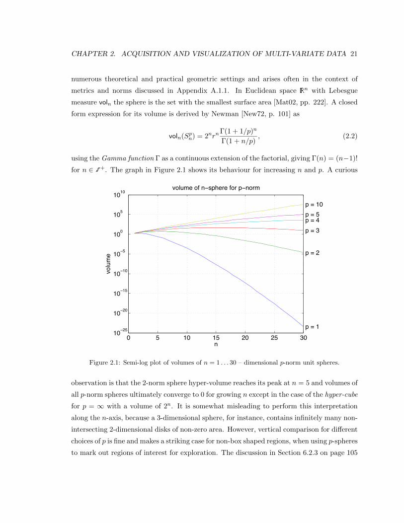
CHAPTER 2. ACQUISITION AND VISUALIZATION OF MULTI-VARIATE DATA 21
numerous theoretical and practical geometric settings and arises often in the context of
metrics and norms discussed in Appendix A.1.1. In Euclidean space Rn with Lebesgue
measure voln the sphere is the set with the smallest surface area [Mat02, pp. 222]. A closed
form expression for its volume is derived by Newman [New72, p. 101] as
voln(Spn) = 2nrnΓ(1 + 1/p)n
Γ(1 + n/p), (2.2)
using the Gamma function Γ as a continuous extension of the factorial, giving Γ(n) = (n−1)!
for n ∈ Z+. The graph in Figure 2.1 shows its behaviour for increasing n and p. A curious
0 5 10 15 20 25 3010−25
10−20
10−15
10−10
10−5
100
105
1010volume of n−sphere for p−norm
n
volu
me
p = 1
p = 2
p = 3p = 4p = 5p = 10
Figure 2.1: Semi-log plot of volumes of n = 1 . . . 30 – dimensional p-norm unit spheres.
observation is that the 2-norm sphere hyper-volume reaches its peak at n = 5 and volumes of
all p-norm spheres ultimately converge to 0 for growing n except in the case of the hyper-cube
for p = ∞ with a volume of 2n. It is somewhat misleading to perform this interpretation
along the n-axis, because a 3-dimensional sphere, for instance, contains infinitely many non-
intersecting 2-dimensional disks of non-zero area. However, vertical comparison for different
choices of p is fine and makes a striking case for non-box shaped regions, when using p-spheres
to mark out regions of interest for exploration. The discussion in Section 6.2.3 on page 105
CHAPTER 2. ACQUISITION AND VISUALIZATION OF MULTI-VARIATE DATA 22
will come back to this aspect. Rearranging Equation 2.2 one obtains the radius
rn =Γ(1 + n/2)1/n
2Γ(3/2)(2.3)
for an n-dimensional 2-norm sphere of unit volume. This radius will be relevant in Sec-
tion 2.3.4 on page 32 to provide an upper bound for the density of periodic sphere packings.
The implications of this discussion are: the more variables or dimensions in a metric
space are to be inspected, the larger is the volume to cover. Volume is directly proportional
to the number of configuration points that need to be computed in order to maintain a
certain density. In most settings, this directly corresponds to computational cost, which we
would like to minimize. One way to do so, is to determine first, how many variables actually
matter. While algorithmic development on this topic is current research not covered in this
thesis, the following brief technical discussion of the issue can provide an entry point in the
future.
Estimating dimensionality: Lebesgue’s covering theorem points out a connection be-
tween the dimensional number n of a region M and the minimum number of n+ 1 simulta-
neous intersections when covering M with small open neighbourhoods. In a metric space one
can use interiors of spheres of radius R for this purpose. Let mR(M) denote the minimum
number of such neighbourhoods of diameter < R needed to cover a set M and note that if
M has an n-dimensional volume, this count fulfills mR(M) ∼ R−n. This is the idea behind
the so-called capacity dimension, also called Hausdorff- or fractal-dimension that estimates
the largest polynomial degree n of the above count for arbitrarily small neighbourhoods as:2
dimcap(M) = − limR→0+
lnmR(M)
lnR. (2.4)
A more easily computed lower bound to this number is given by the correlation dimension.3
It is also considered as a measure of intrinsic dimension by Levina and Bickel [LB05]. To
allow for a statistical analysis, they construct a Poisson process for the point set that is uni-
formly distributed inside M counting the number of points that lie within a growing radius
2Note that this works for any non-zero volume of M , as it comes out of the logarithm in the enumeratoras an additive constant and then vanishes against the magnitude of the denominator.
3The correlation dimension [Wei09] is counting pairs of points of a set M within a radius R of each other asa measure of connectedness. This count rises in the order of Rn, with the monomial degree n correspondingto the correlation dimension dimcor(M).
CHAPTER 2. ACQUISITION AND VISUALIZATION OF MULTI-VARIATE DATA 23
of each other. The growth rate of this process depends on the local density, dimensionality,
and implicitly the sphere volume Vn = voln(S2n) derived in Equation 2.2. Based on this, a
closed form solution is derived for the maximum likelihood estimate of the dimensionality
that is averaged over all points of M . Their discussion points out that dimension may vary
with position x and with a choice of scale, which is specified in their method by either a
maximum radius or an index of the k-furthest neighbour to consider in the estimate.
Beyond these geometric perspectives on dimensionality, the approximation of functions
in linear spaces also requires choices of sample points for which a discussion is provided in
Appendix A.2. This setting can be interpreted as looking at a family of integrals — one
member for each point to reconstruct. The following discussion more specifically considers
the computation of a single integral.
2.2 Quadrature error
An important class of integration methods are the so-called quadrature (or cubature) rules
that approximate an integral of a function f over a finite domain M ⊂ Rn as a weighted
sum of point samples in a set X ⊂M of size m = |X|
If =
∫Mf(x)dnx ≈ Qf =
∑xk∈X
wkf(xk). (2.5)
Different choices for X and w distinguish the respective integration methods. For instance,
consider a factorial design, e.g., implemented via nested for-loops that iterate each com-
ponent variable xi of the vectors x ∈ X over a set of values Xi. This leads to an overall
number of m =∏ni=1 |Xi| points. Even if only two distinct values per variable are desired,
this design has m = 2n points, growing exponentially in the number of variables. We will
mainly focus on the placement of the points and assume uniform weights w = 1m . However,
prepending a brief discussion of non-uniform weighting will help to illustrate a basic effect.
Using a linear function space model, the integrand f is approximated by a sum of basis
functions (see Appendix B.2, also Appendix B.2.2 or Phillips [Phi03, pp. 119])). This linear
model determines the weighted contribution wk that each point sample has to the integral
estimate. More specifically, the composite Newton-Cotes method uses Lagrange polynomials
of degree s < m to properly represent a certain level of smoothness of the integrand.
The resulting error term is proportional to hs+2f (s+1)(ξ) for some point ξ contained in
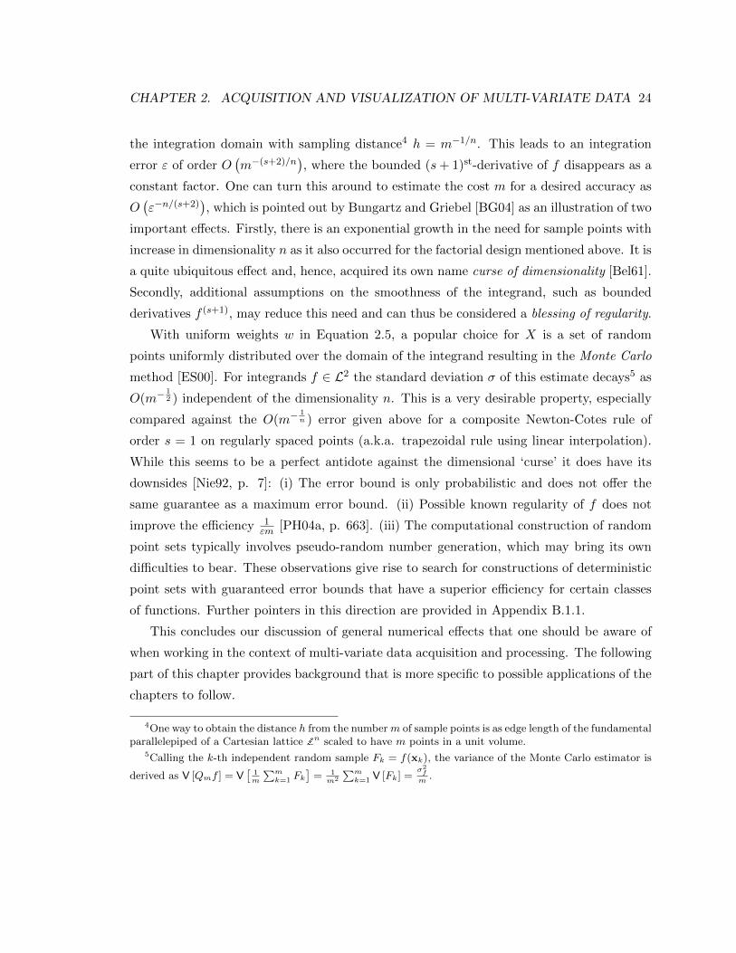
CHAPTER 2. ACQUISITION AND VISUALIZATION OF MULTI-VARIATE DATA 24
the integration domain with sampling distance4 h = m−1/n. This leads to an integration
error ε of order O(m−(s+2)/n
), where the bounded (s+ 1)st-derivative of f disappears as a
constant factor. One can turn this around to estimate the cost m for a desired accuracy as
O(ε−n/(s+2)
), which is pointed out by Bungartz and Griebel [BG04] as an illustration of two
important effects. Firstly, there is an exponential growth in the need for sample points with
increase in dimensionality n as it also occurred for the factorial design mentioned above. It is
a quite ubiquitous effect and, hence, acquired its own name curse of dimensionality [Bel61].
Secondly, additional assumptions on the smoothness of the integrand, such as bounded
derivatives f (s+1), may reduce this need and can thus be considered a blessing of regularity.
With uniform weights w in Equation 2.5, a popular choice for X is a set of random
points uniformly distributed over the domain of the integrand resulting in the Monte Carlo
method [ES00]. For integrands f ∈ L2 the standard deviation σ of this estimate decays5 as
O(m−12 ) independent of the dimensionality n. This is a very desirable property, especially
compared against the O(m−1n ) error given above for a composite Newton-Cotes rule of
order s = 1 on regularly spaced points (a.k.a. trapezoidal rule using linear interpolation).
While this seems to be a perfect antidote against the dimensional ‘curse’ it does have its
downsides [Nie92, p. 7]: (i) The error bound is only probabilistic and does not offer the
same guarantee as a maximum error bound. (ii) Possible known regularity of f does not
improve the efficiency 1εm [PH04a, p. 663]. (iii) The computational construction of random
point sets typically involves pseudo-random number generation, which may bring its own
difficulties to bear. These observations give rise to search for constructions of deterministic
point sets with guaranteed error bounds that have a superior efficiency for certain classes
of functions. Further pointers in this direction are provided in Appendix B.1.1.
This concludes our discussion of general numerical effects that one should be aware of
when working in the context of multi-variate data acquisition and processing. The following
part of this chapter provides background that is more specific to possible applications of the
chapters to follow.
4One way to obtain the distance h from the numberm of sample points is as edge length of the fundamentalparallelepiped of a Cartesian lattice Zn scaled to have m points in a unit volume.
5Calling the k-th independent random sample Fk = f(xk), the variance of the Monte Carlo estimator is
derived as V [Qmf ] = V[
1m
∑mk=1 Fk
]= 1
m2
∑mk=1 V [Fk] =
σ2f
m.
CHAPTER 2. ACQUISITION AND VISUALIZATION OF MULTI-VARIATE DATA 25
2.3 Discretization of multi-dimensional functions
As pointed out in the data abstraction Section 1.4, we view a simulation model as a function
f with deterministic code to compute it. In order to apply the visualization techniques that
will be pointed out in Section 2.4, we first need to turn this functional representation into
a finite, discrete data set.
The setting of numerical integration has already been introduced in Section 2.2. Another
operation required for digital numerical representation is quantization. Often also referred to
as clustering, it obtains a discrete representation of a probability distribution over a metric
space, which involves criteria discussed in Section 2.3.1.2. While quantization of the range
of f typically incurs some loss of information, discretization of its domain can in certain
cases be perfectly undone. The theory related to this topic of reconstruction and prediction
of unobserved points is reviewed from the angle of signal processing and approximation
theory in Appendix B.2 with a statistical perspective from the field of experimental design
provided in Section 2.3.2.
2.3.1 Useful concepts for metric data representation
First, some basic constructs are defined that will find application in later chapters.
2.3.1.1 Voronoi cells and the Delaunay graph
A basic construct when studying point set geometry is the nearest neighbour cell of a sample
point, also denoted as Voronoi cell. It contains the portion of space around a point that is
closer to this point than to any other one. An illustration of what this means geometrically
is given in Figure 2.2. Algebraically, such a cell around a point xk ∈ X is defined as
Ω(xk) = x ∈ Rn : ‖x− xk‖ ≤ ‖x− u‖ for all u ∈ X. (2.6)
The boundary of this region is formed by bisecting hyperplanes between xk and the Voronoi
relevant neighbours
N(xk) = 2Ω(xk)− xk ∩X, (2.7)
namely all points of X that are covered when uniformly scaling Ω(xk) around xk by a factor
of 2.
CHAPTER 2. ACQUISITION AND VISUALIZATION OF MULTI-VARIATE DATA 26
Figure 2.2: Set of 20 randomly distributed sample points in [0, 1]2 with Voronoi regions outlined inblue and Voronoi relevant neighbours connected by grey lines. Notice how the convex hull and theminimum spanning tree are part of the grey Delaunay graph connecting Voronoi relevant neighbours.For points in general position the Delaunay graph turns out to be a triangulation or a simplicialcomplex in higher-dimensional spaces.
2.3.1.2 Measuring quantization error via the second order moment
A partition of the continuous domain into a finite number of cells can be used to analyze
the action of a quantizer that rounds each point in Rn to the nearest quantization site
in X. This application motivates a first quality measure for the set X. The normalized,
dimensionless second order moment of inertia measures the mean squared error (MSE) per
quantized symbol6 [CS82, Eq. 8],[CS99, Ch. 21]
Gn(Ω(xk)) =1
n
∫Ω(xk)‖x− xk‖2dnx
voln(Ω (xk))(n+2)/n
, (2.8)
for signals that are uniformly distributed over the range containing Ω(xk). This figure is
lowest for a sphere and may also serve as a measure for sphere dissimilarity of the Voronoi
region. The functional that computes the MSE Gn(X) for the entire domain of the quantizer
X, is formed as a sum of the second order moments of each of the Voronoi cells of the points
in X. It can be computed analytically with the method of Appendix A.1.3 and is applied
in the context of Figure 3.2 on page 54.
6The root of this error (RMSE) would be in the unit of the original distance measure and is numericallyeasier to interpret. We keep the squared form, since it is mathematically easier derive from.
CHAPTER 2. ACQUISITION AND VISUALIZATION OF MULTI-VARIATE DATA 27
Numerical relaxation: The idea underlying Lloyd’s algorithm [Llo82] is to iteratively
improve a quantizer X by moving the quantization sites xk to the centers of their Voronoi
regions. Convergence of this algorithm has been analyzed for one-dimensional [SG86] and
two-dimensional settings [DEJ06], but is still open for quantization in higher-dimensional
spaces. Lloyd’s algorithm can also be studied as a dynamical system [CB09], e.g., of agents
maximizing their mutual distances from each other, with interesting patterns for the tra-
jectories of the point locations that arise from using different approximations to the true
Voronoi cell centroid as local attractor. The algorithm has numerous applications, including
half-toning [BSD09, Han05], photon-tracing [SJ09], and the optimization of experimental
designs [HA02]. The latter is due to the fact that the mean squared quantization error when
representing a region with a point as in Equation 2.8 is minimized when this representative
point is the centroid of the region. An alternative to numerical optimization is to directly
construct a quantizer that is a local optimum of the second moment error functional, i.e.
that is a fixed point of Lloyd’s algorithm. An important example of that is given in the
following.
2.3.1.3 Sampling lattices
For any periodic structure that can be seen as n-dimensional, additive subgroup of Rn, it is
possible to construct a set of basis vectors [Mat02, p. 22] whose integer multiples generate
the set of periods or self-similar displacements of the structure. This set is referred to as
point lattice7 Λ. Such a set Λ is defined as subset of Rn that is closed under addition and
inversion
Λ(G) = Gk : k ∈ Zn ⊂ Rn. (2.9)
Its non-singular generating matrix G ∈ Rn×n is omitted as an argument if it is clear from
context. To retain the uniqueness of k, we exclude non-square G of rank n from consider-
ation. Scaling and angles between the basis column vectors of G are implicitly represented
by its Gram matrix
A = GTG. (2.10)
7This has nothing to do with the algebraic structure called lattice that refers to a partially ordered setwith a unique infimum and supremum. A collision could occur when talking about the face lattice of apolytope that represents containment of vertices, edges, or facets (see Appendix A.1). The attributes point-or sampling lattice both refer to the above definition.
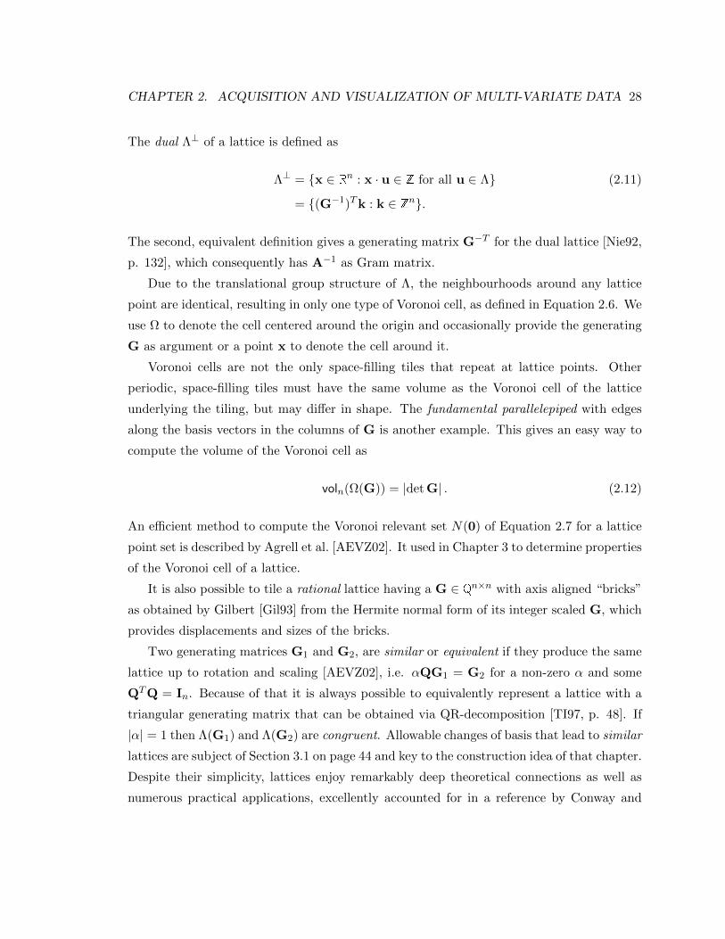
CHAPTER 2. ACQUISITION AND VISUALIZATION OF MULTI-VARIATE DATA 28
The dual Λ⊥ of a lattice is defined as
Λ⊥ = x ∈ Rn : x · u ∈ Z for all u ∈ Λ (2.11)
= (G−1)Tk : k ∈ Zn.
The second, equivalent definition gives a generating matrix G−T for the dual lattice [Nie92,
p. 132], which consequently has A−1 as Gram matrix.
Due to the translational group structure of Λ, the neighbourhoods around any lattice
point are identical, resulting in only one type of Voronoi cell, as defined in Equation 2.6. We
use Ω to denote the cell centered around the origin and occasionally provide the generating
G as argument or a point x to denote the cell around it.
Voronoi cells are not the only space-filling tiles that repeat at lattice points. Other
periodic, space-filling tiles must have the same volume as the Voronoi cell of the lattice
underlying the tiling, but may differ in shape. The fundamental parallelepiped with edges
along the basis vectors in the columns of G is another example. This gives an easy way to
compute the volume of the Voronoi cell as
voln(Ω(G)) = |det G| . (2.12)
An efficient method to compute the Voronoi relevant set N(0) of Equation 2.7 for a lattice
point set is described by Agrell et al. [AEVZ02]. It used in Chapter 3 to determine properties
of the Voronoi cell of a lattice.
It is also possible to tile a rational lattice having a G ∈ Qn×n with axis aligned “bricks”
as obtained by Gilbert [Gil93] from the Hermite normal form of its integer scaled G, which
provides displacements and sizes of the bricks.
Two generating matrices G1 and G2, are similar or equivalent if they produce the same
lattice up to rotation and scaling [AEVZ02], i.e. αQG1 = G2 for a non-zero α and some
QTQ = In. Because of that it is always possible to equivalently represent a lattice with a
triangular generating matrix that can be obtained via QR-decomposition [TI97, p. 48]. If
|α| = 1 then Λ(G1) and Λ(G2) are congruent. Allowable changes of basis that lead to similar
lattices are subject of Section 3.1 on page 44 and key to the construction idea of that chapter.
Despite their simplicity, lattices enjoy remarkably deep theoretical connections as well as
numerous practical applications, excellently accounted for in a reference by Conway and
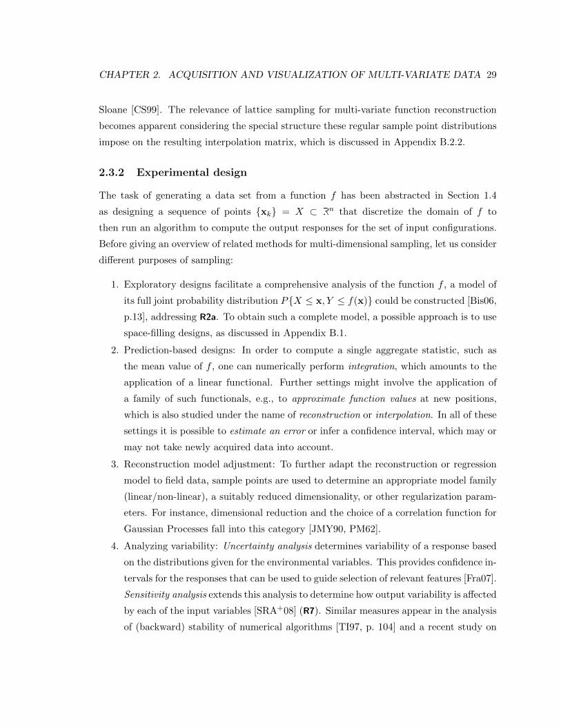
CHAPTER 2. ACQUISITION AND VISUALIZATION OF MULTI-VARIATE DATA 29
Sloane [CS99]. The relevance of lattice sampling for multi-variate function reconstruction
becomes apparent considering the special structure these regular sample point distributions
impose on the resulting interpolation matrix, which is discussed in Appendix B.2.2.
2.3.2 Experimental design
The task of generating a data set from a function f has been abstracted in Section 1.4
as designing a sequence of points xk = X ⊂ Rn that discretize the domain of f to
then run an algorithm to compute the output responses for the set of input configurations.
Before giving an overview of related methods for multi-dimensional sampling, let us consider
different purposes of sampling:
1. Exploratory designs facilitate a comprehensive analysis of the function f , a model of
its full joint probability distribution PX ≤ x, Y ≤ f(x) could be constructed [Bis06,
p.13], addressing R2a. To obtain such a complete model, a possible approach is to use
space-filling designs, as discussed in Appendix B.1.
2. Prediction-based designs: In order to compute a single aggregate statistic, such as
the mean value of f , one can numerically perform integration, which amounts to the
application of a linear functional. Further settings might involve the application of
a family of such functionals, e.g., to approximate function values at new positions,
which is also studied under the name of reconstruction or interpolation. In all of these
settings it is possible to estimate an error or infer a confidence interval, which may or
may not take newly acquired data into account.
3. Reconstruction model adjustment: To further adapt the reconstruction or regression
model to field data, sample points are used to determine an appropriate model family
(linear/non-linear), a suitably reduced dimensionality, or other regularization param-
eters. For instance, dimensional reduction and the choice of a correlation function for
Gaussian Processes fall into this category [JMY90, PM62].
4. Analyzing variability: Uncertainty analysis determines variability of a response based
on the distributions given for the environmental variables. This provides confidence in-
tervals for the responses that can be used to guide selection of relevant features [Fra07].
Sensitivity analysis extends this analysis to determine how output variability is affected
by each of the input variables [SRA+08] (R7). Similar measures appear in the analysis
of (backward) stability of numerical algorithms [TI97, p. 104] and a recent study on
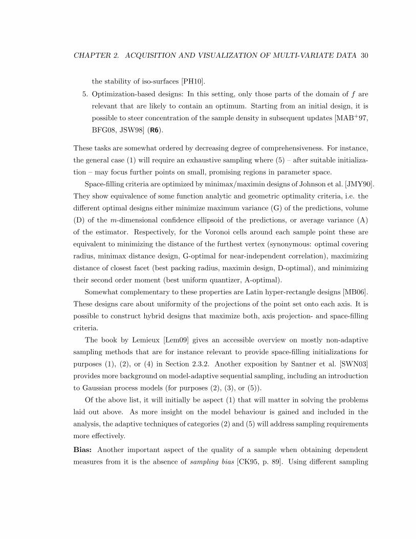
CHAPTER 2. ACQUISITION AND VISUALIZATION OF MULTI-VARIATE DATA 30
the stability of iso-surfaces [PH10].
5. Optimization-based designs: In this setting, only those parts of the domain of f are
relevant that are likely to contain an optimum. Starting from an initial design, it is
possible to steer concentration of the sample density in subsequent updates [MAB+97,
BFG08, JSW98] (R6).
These tasks are somewhat ordered by decreasing degree of comprehensiveness. For instance,
the general case (1) will require an exhaustive sampling where (5) – after suitable initializa-
tion – may focus further points on small, promising regions in parameter space.
Space-filling criteria are optimized by minimax/maximin designs of Johnson et al. [JMY90].
They show equivalence of some function analytic and geometric optimality criteria, i.e. the
different optimal designs either minimize maximum variance (G) of the predictions, volume
(D) of the m-dimensional confidence ellipsoid of the predictions, or average variance (A)
of the estimator. Respectively, for the Voronoi cells around each sample point these are
equivalent to minimizing the distance of the furthest vertex (synonymous: optimal covering
radius, minimax distance design, G-optimal for near-independent correlation), maximizing
distance of closest facet (best packing radius, maximin design, D-optimal), and minimizing
their second order moment (best uniform quantizer, A-optimal).
Somewhat complementary to these properties are Latin hyper-rectangle designs [MB06].
These designs care about uniformity of the projections of the point set onto each axis. It is
possible to construct hybrid designs that maximize both, axis projection- and space-filling
criteria.
The book by Lemieux [Lem09] gives an accessible overview on mostly non-adaptive
sampling methods that are for instance relevant to provide space-filling initializations for
purposes (1), (2), or (4) in Section 2.3.2. Another exposition by Santner et al. [SWN03]
provides more background on model-adaptive sequential sampling, including an introduction
to Gaussian process models (for purposes (2), (3), or (5)).
Of the above list, it will initially be aspect (1) that will matter in solving the problems
laid out above. As more insight on the model behaviour is gained and included in the
analysis, the adaptive techniques of categories (2) and (5) will address sampling requirements
more effectively.
Bias: Another important aspect of the quality of a sample when obtaining dependent
measures from it is the absence of sampling bias [CK95, p. 89]. Using different sampling
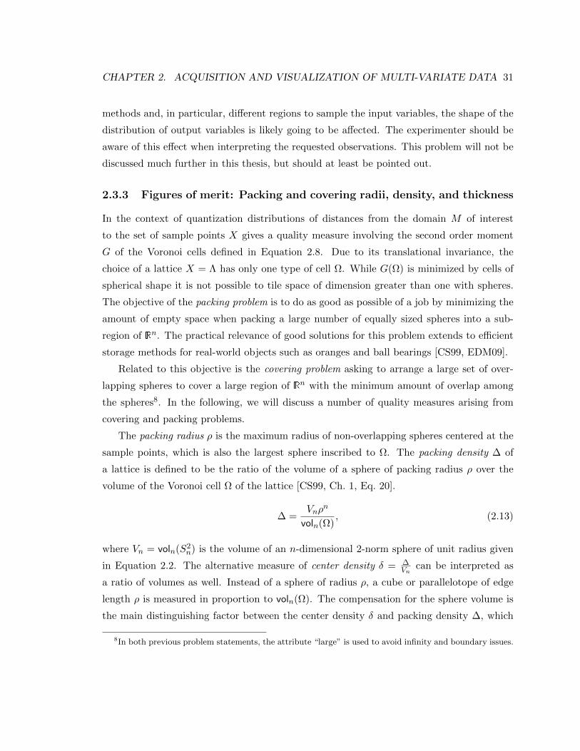
CHAPTER 2. ACQUISITION AND VISUALIZATION OF MULTI-VARIATE DATA 31
methods and, in particular, different regions to sample the input variables, the shape of the
distribution of output variables is likely going to be affected. The experimenter should be
aware of this effect when interpreting the requested observations. This problem will not be
discussed much further in this thesis, but should at least be pointed out.
2.3.3 Figures of merit: Packing and covering radii, density, and thickness
In the context of quantization distributions of distances from the domain M of interest
to the set of sample points X gives a quality measure involving the second order moment
G of the Voronoi cells defined in Equation 2.8. Due to its translational invariance, the
choice of a lattice X = Λ has only one type of cell Ω. While G(Ω) is minimized by cells of
spherical shape it is not possible to tile space of dimension greater than one with spheres.
The objective of the packing problem is to do as good as possible of a job by minimizing the
amount of empty space when packing a large number of equally sized spheres into a sub-
region of Rn. The practical relevance of good solutions for this problem extends to efficient
storage methods for real-world objects such as oranges and ball bearings [CS99, EDM09].
Related to this objective is the covering problem asking to arrange a large set of over-
lapping spheres to cover a large region of Rn with the minimum amount of overlap among
the spheres8. In the following, we will discuss a number of quality measures arising from
covering and packing problems.
The packing radius ρ is the maximum radius of non-overlapping spheres centered at the
sample points, which is also the largest sphere inscribed to Ω. The packing density ∆ of
a lattice is defined to be the ratio of the volume of a sphere of packing radius ρ over the
volume of the Voronoi cell Ω of the lattice [CS99, Ch. 1, Eq. 20].
∆ =Vnρ
n
voln(Ω), (2.13)
where Vn = voln(S2n) is the volume of an n-dimensional 2-norm sphere of unit radius given
in Equation 2.2. The alternative measure of center density δ = ∆Vn
can be interpreted as
a ratio of volumes as well. Instead of a sphere of radius ρ, a cube or parallelotope of edge
length ρ is measured in proportion to voln(Ω). The compensation for the sphere volume is
the main distinguishing factor between the center density δ and packing density ∆, which
8In both previous problem statements, the attribute “large” is used to avoid infinity and boundary issues.
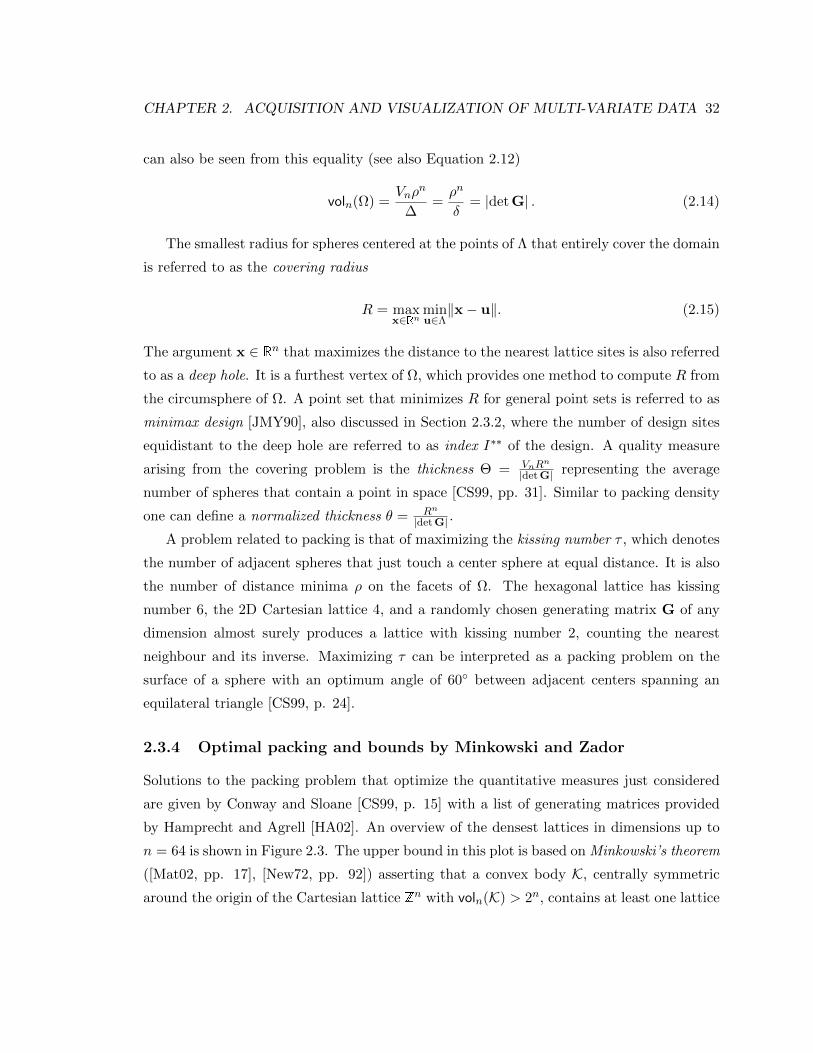
CHAPTER 2. ACQUISITION AND VISUALIZATION OF MULTI-VARIATE DATA 32
can also be seen from this equality (see also Equation 2.12)
voln(Ω) =Vnρ
n
∆=ρn
δ= |det G| . (2.14)
The smallest radius for spheres centered at the points of Λ that entirely cover the domain
is referred to as the covering radius
R = maxx∈Rn
minu∈Λ‖x− u‖. (2.15)
The argument x ∈ Rn that maximizes the distance to the nearest lattice sites is also referred
to as a deep hole. It is a furthest vertex of Ω, which provides one method to compute R from
the circumsphere of Ω. A point set that minimizes R for general point sets is referred to as
minimax design [JMY90], also discussed in Section 2.3.2, where the number of design sites
equidistant to the deep hole are referred to as index I∗∗ of the design. A quality measure
arising from the covering problem is the thickness Θ = VnRn
|det G| representing the average
number of spheres that contain a point in space [CS99, pp. 31]. Similar to packing density
one can define a normalized thickness θ = Rn
|det G| .
A problem related to packing is that of maximizing the kissing number τ , which denotes
the number of adjacent spheres that just touch a center sphere at equal distance. It is also
the number of distance minima ρ on the facets of Ω. The hexagonal lattice has kissing
number 6, the 2D Cartesian lattice 4, and a randomly chosen generating matrix G of any
dimension almost surely produces a lattice with kissing number 2, counting the nearest
neighbour and its inverse. Maximizing τ can be interpreted as a packing problem on the
surface of a sphere with an optimum angle of 60 between adjacent centers spanning an
equilateral triangle [CS99, p. 24].
2.3.4 Optimal packing and bounds by Minkowski and Zador
Solutions to the packing problem that optimize the quantitative measures just considered
are given by Conway and Sloane [CS99, p. 15] with a list of generating matrices provided
by Hamprecht and Agrell [HA02]. An overview of the densest lattices in dimensions up to
n = 64 is shown in Figure 2.3. The upper bound in this plot is based on Minkowski’s theorem
([Mat02, pp. 17], [New72, pp. 92]) asserting that a convex body K, centrally symmetric
around the origin of the Cartesian lattice Zn with voln(K) > 2n, contains at least one lattice
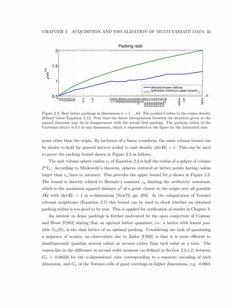
CHAPTER 2. ACQUISITION AND VISUALIZATION OF MULTI-VARIATE DATA 33
0.5
1
1.5
2Packing radii
!="1/
n
n
Z A2 A3 D4 D5 E6 E7 E8 K12
L16
L24
L25
L26
B27
B28
B29
Q30
Q31
Q32
Q33
Q34 B35
KS36 D37
D38
P48_
39P4
8_40
P48_
41P4
8_42
P48_
43P4
8_44
P48_
45P4
8_46
P48_
47 P48
MW
54 L56
NE64
densest known latticesarithmetic minimum upper bound rn
Figure 2.3: Best lattice packings in dimensions n = 1 . . . 64. The symbol δ refers to the center densitydefined below Equation 2.13. Note that the linear interpolation between the densities given at thenamed abscissae may be in disagreement with the actual best packing. The packing radius of theCartesian lattice is 0.5 in any dimension, which is represented in the figure by the horizontal axis.
point other than the origin. By inclusion of a linear transform, the same volume bound can
be shown to hold for general lattices scaled to unit density |det G| = 1. This can be used
to prove the packing bound shown in Figure 2.3 as follows.
The unit volume sphere radius rn of Equation 2.3 is half the radius of a sphere of volume
2nVn. According to Minkowski’s theorem, spheres centered at lattice points having radius
larger than rn have to intersect. This provides the upper bound for ρ shown in Figure 2.3.
The bound is directly related to Hermite’s constant γn limiting the arithmetic minimum,
which is the maximum squared distance ρ2 of a point closest to the origin over all possible
ΛG with |det G| = 1 in n-dimensions [New72, pp. 202]. In the computation of Voronoi
relevant neighbours (Equation 2.7) this bound can be used to check whether an obtained
packing radius is too good to be true. This is applied for verification of results in Chapter 3.
An interest in dense packings is further motivated by the open conjecture of Conway
and Sloan [CS82] stating that an optimal lattice quantizer, i.e. a lattice with lowest pos-
sible Gn(Ω), is the dual lattice of an optimal packing. Considering the task of quantizing
a sequence of scalars, an observation due to Zador [CS85] is that it is more efficient to
simultaneously quantize several values as vectors rather than each value at a time. The
reason lies in the difference in second order moment (as defined in Section 2.3.1.2) between
Gn = 0.08333 for the n-dimensional cube corresponding to a separate encoding of each
dimension, and Gn of the Voronoi cells of good coverings in higher dimensions, e.g., 0.0801
CHAPTER 2. ACQUISITION AND VISUALIZATION OF MULTI-VARIATE DATA 34
0 5 10 15 20 25
123456789
10
Zador’s upper bound for MSEof n−dimensional optimal quantizer
n
100*
Gn
upperlower (sphere)CC (cube)
Figure 2.4: Zador’s bounds for the mean squared quantization error of optimal quantizers in Rn.
for the hexagon, 0.0785 for the truncated octahedron of BCC, or 0.0657 for the Voronoi
cell of the 24-dimensional Leech lattice. Each of these figures directly corresponds to the
mean squared error per symbol when encoding chunks of 2, 3, or 24 numbers by the nearest
points on the respective lattice. A plot of Zador’s bound as summarized by Conway [CS85]
is shown in Figure 2.4. The derivation of the upper bound, as described by Zador [Zad82,
Eq. 16-23 and 43], involve the second moment of the distribution of round-off errors of a
uniform random quantizer with a large number m of quantization sites. For m → ∞ it
converges to the second moment of an n-dimensional sphere, which serves as lower bound
for any optimal quantizer and is shown as green line in Figure 2.4.
2.4 Visual interfaces for multi-variate computer model data
The discussion in Section 1 has remarked that computational models in domains of human
interest significantly benefit from good human interfaces. Regardless of their domain, the
development of any computer model has to go through certain stages including to convince
developers and users of its validity. At a basic level, this concerns development methodology
CHAPTER 2. ACQUISITION AND VISUALIZATION OF MULTI-VARIATE DATA 35
and the choice of programming language9, but this topic is explored further here.
In Section 1 a point was made for using the visual channel in order to create efficient
interfaces. The visualization process [dSB04, HM90, CJ10] classically starts with a given
data set, possibly performing further refinement or filtering to then map data points to
graphical primitives that are subsequently rendered to the screen. Recent work by Chen and
Janicke [CJ10] considers an information theoretic perspective on the visualization pipeline.
Their survey of applicable theory from that domain proposes a unified view on the amount
of information that a particular data set provides relative to a set of possible ones, and, in
the same light, how much information different visual mappings (e.g., overview and detail)
of a data set provide in relationship to each other. This promising abstraction opens up
several directions for further pursuit by the visualization community: a) A large size for
an encoding is bad by typical information theoretic notions. However, as pointed out by
the authors, a large image may be significantly easier to read than a small one. In general,
what matters for the comprehension of a visualization is the computational or temporal
complexity of the decoding procedure, probably more so than the spatial complexity of the
code. b) Information measures based on entropy typically are sensitive to noise, since it is
rated as something unexpected and in that is similar to valuable information. A possible
extension of this work could attempt to make distinctions between relevant and irrelevant
information, as it could for instance be derived from a driving question or task. The task
overview that will be given in Section 2.4.1 can be seen as a first step into a task-driven
organization of research. However, it is focussed on interacting with computer models,
rather than visualization algorithms.
With data input at one end of the visualization process and the human observer at
the other it is natural to start by looking at the quality of the input. The first part of
this chapter did this from a numerical perspective, where two main factors where discussed
that impact sample complexity: the volume of the region to cover (Section 2.1) and the
uniformity of the point distribution that is generated inside a given region (Section 2.3.2).
Beyond numerical point data, the following distinction of data types provides a possible
structure to the visualization research landscape.
9Choices of high-level scripting languages, such as Python or MATLAB (see also Section 6.2.1)can already be considered among the human-friendly ones. See http://www.webmonkey.com/2011/02/
cussing-in-commits-which-programming-language-inspires-the-most-swearing/ for a humorous sta-tistical argument in this direction. However, having noted the issue of bias earlier, in this sample differentlanguages imply different types of problems programmers are working on.
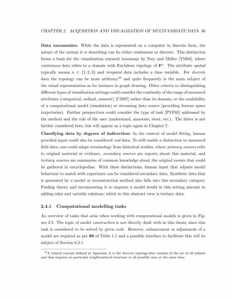
CHAPTER 2. ACQUISITION AND VISUALIZATION OF MULTI-VARIATE DATA 36
Data taxonomies: While the data is represented on a computer in discrete form, the
nature of the system it is describing can be either continuous or discrete. This distinction
forms a basis for the visualization research taxonomy by Tory and Moller [TM04], where
continuous data refers to a domain with Euclidean topology of Rn. The attribute spatial
typically means n ∈ 1, 2, 3 and temporal data includes a time variable. For discrete
data the topology can be more arbitrary10 and quite frequently is the main subject of
the visual representation as for instance in graph drawing. Other criteria to distinguishing
different types of visualization settings could consider the continuity of the range of measured
attributes (categorical, ordinal, numeric) [CM97] rather than its domain, or the availability
of a computational model (simulation) or streaming data source (providing feature space
trajectories). Further perspectives could consider the type of task [PVF05] addressed by
the method and the role of the user (understand, annotate, steer, etc.). The latter is not
further considered here, but will appear as a topic again in Chapter 7.
Classifying data by degrees of indirection: In the context of model fitting, human
provided input could also be considered real data. To still enable a distinction to measured
field data, one could adapt terminology from historical studies, where primary sources refer
to original material or evidence, secondary sources are reports about this material, and
tertiary sources are summaries of common knowledge about the original events that could
be gathered in encyclopedias. With these distinctions, human input that adjusts model
behaviour to match with experience can be considered secondary data. Synthetic data that
is generated by a model or reconstruction method also falls into this secondary category.
Finding theory and incorporating it to improve a model would in this setting amount to
adding rules and variable relations, which in this abstract view is tertiary data.
2.4.1 Computational modelling tasks
An overview of tasks that arise when working with computational models is given in Fig-
ure 2.5. The topic of model construction is not directly dealt with in this thesis, since this
task is considered to be solved by given code. However, enhancement or adjustment of a
model are required as per R4 of Table 1.1 and a possible interface to facilitate this will be
subject of Section 6.2.1.
10A related concept defined in Appendix A is the discrete topology that consists of the set of all subsetsand thus imposes no particular neighbourhood structure or all possible ones at the same time.
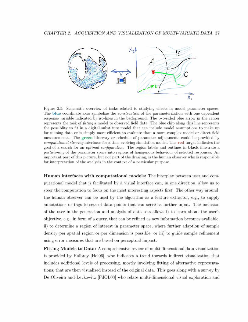
CHAPTER 2. ACQUISITION AND VISUALIZATION OF MULTI-VARIATE DATA 37
Figure 2.5: Schematic overview of tasks related to studying effects in model parameter spaces.The blue coordinate axes symbolize the construction of the parameterization with one dependentresponse variable indicated by iso-lines in the background. The two-sided blue arrow in the centerrepresents the task of fitting a model to observed field data. The blue chip along this line representsthe possiblity to fit in a digital substitute model that can include model assumptions to make upfor missing data or is simply more efficient to evaluate than a more complex model or direct fieldmeasurements. The green itinerary or schedule of parameter adjustments could be provided bycomputational steering interfaces for a time-evolving simulation model. The red target indicates thegoal of a search for an optimal configuration. The region labels and outlines in black illustrate apartitioning of the parameter space into regions of homgenous behaviour of selected responses. Animportant part of this picture, but not part of the drawing, is the human observer who is responsiblefor interpretation of the analysis in the context of a particular purpose.
Human interfaces with computational models: The interplay between user and com-
putational model that is facilitated by a visual interface can, in one direction, allow us to
steer the computation to focus on the most interesting aspects first. The other way around,
the human observer can be used by the algorithm as a feature extractor, e.g., to supply
annotations or tags to sets of data points that can serve as further input. The inclusion
of the user in the generation and analysis of data sets allows i) to learn about the user’s
objective, e.g., in form of a query, that can be refined as new information becomes available,
ii) to determine a region of interest in parameter space, where further adaption of sample
density per spatial region or per dimension is possible, or iii) to guide sample refinement
using error measures that are based on perceptual impact.
Fitting Models to Data: A comprehensive review of multi-dimensional data visualization
is provided by Holbrey [Hol06], who indicates a trend towards indirect visualization that
includes additional levels of processing, mostly involving fitting of alternative representa-
tions, that are then visualized instead of the original data. This goes along with a survey by
De Oliveira and Levkowitz [FdOL03] who relate multi-dimensional visual exploration and

CHAPTER 2. ACQUISITION AND VISUALIZATION OF MULTI-VARIATE DATA 38
data mining, observing a need for methods that more tightly integrate visualization and
analysis. This recent trend to use visualization methods to make data analysis algorithms
more understandable is pursued by Wickham [Wic08], discussing the usage of statistical
models on top of the given data. To sharpen the terminology, a distinction is made between
the family of a model (linear regression, clustering, etc.), the form (which variables are
factors or responses), and the fitted model finally refers to a particular instance adapted to
the underlying data. Some characteristic tasks that are encountered in visual data mining
are recognized by Himberg [Him04], including predictive modelling, descriptive modelling,
discovering rules and patterns, exploratory data analysis, and retrieval by content.
Data-centric visualization research: Since multi-dimensional numeric data is the result
of discretizing the parameter space of the types of computational models considered in Sec-
tion 1.2 any applicable visualization technique should support it. To determine the relative
interest of the visualization community in multi-dimensional data, a survey of publications
of the three conferences of IEEE VisWeek 2008 has been assembled. A grouping by data
set type11 gives the following distribution of paper counts:
• Vis: scalar volumes (12), flow and tensor (8), general multi-field12 (6), segmented
data (2), surface models (15)
• InfoVis: Graphs/Trees (14), (multi-)relational tables (8), continuous/spatio-temporal (3)
• VAST: (Geo-)spatial (2), time stamped feature space trajectories (3), relational ta-
bles (5), integrating mixed types (6)
The first three categories of the visualization conference alone amount to over 26 publi-
cations that deal with data originating from continuous models. Most of the models are
computational and likely would allow for user adjustment of configuration parameters.
To provide quick pointers to further background discussions, related work specific to
certain design components of the paraglide system are embedded in Section 6.2. Work related
to the spectral palette design use case described in Section 1.2.4.2 is discussed in Section 5.1.
11A raw text form of this informal supplementary survey is available at http://www.cs.sfu.ca/~sbergner/personal/proj/thesis/dataset-survey.html
12See Section 1.4 for a definition.

CHAPTER 2. ACQUISITION AND VISUALIZATION OF MULTI-VARIATE DATA 39
2.4.2 Reconstruction and refinement of spatial data
Reconstruction takes a discrete data set as input and fits to it a continuous model that
can be queried at any position of its domain. Intermediate continuous representations are
an integral part of any volume rendering algorithm [HHS94]. For reasons mentioned at
end of Section 2.3.1.3 regular sampling lattices have been the method of choice for this
application [EDM09]. Due to the uniform neighbourhood structure, regular sampling is
also amenable to parallel processing, enabling fast reconstruction and rendering on the
GPU [EKE01a, KPH+03]. For efficient projection, also randomized arrangements of data
points have merit as can be seen in Monte-Carlo volume rendering [CSK03].
Reconstructing continuous density functions: Instead of reconstructing a continuous
function that fits the given data points, it is also possible to compute a continuous descrip-
tion of the density distribution of its range (histogram) or the combined domain×range
space. The projection to one- or two-dimensional subspaces for presentation on the screen
amounts to computing so-called marginal or dependent probabilities. The classical ap-
proach of kernel density estimation [Bis06, Ch. 2] is a distant relative to point based splat-
ting [Wes90, MMC99, HE03] with additive compositing, where spherical reconstruction
kernels are projected to image space prior to interpolation. Novotny and Hauser [NH06]
pre-process and bin a data set into 2D histograms for each pair of dimensions. This data
structure is useful for speeding up rendering of parallel coordinates [BBPD08], but could
also be used to render discretized scatterplots.
If input/output relationships are known : An alternative to value-based binning is
to use sample point adjacency information to project kernels for each cell rather than each
response value, as published by Bachtaler and Weiskopf [BW08] to reconstruct a continuous
density for display in a scatter plot13. Similar to Scheidegger et al. [SSD+08] they use
the co-area formula from level-set theory to obtain an asymptotically accurate histogram
computation for continuous domains.
Also exploiting an input-output relationship, Adams et al. [ABD10] provide a com-
putational representation for multi-dimensional continuous phenomena based on a regular
simplicial decomposition of the domain, where the vertices of each simplex lie on the permu-
tohedral lattice (dual of d-dimensional root lattice Ad [CS99]). Barycentric weights for any
13A related observation that I communicated to the second author in March 2007 is described in Sec-tion 6.2.2.3.
CHAPTER 2. ACQUISITION AND VISUALIZATION OF MULTI-VARIATE DATA 40
given point in space are used as multi-dimensional analysis and reconstruction filter. Since
the permutohedral lattice is a projection of the separable Zd+1 lattice, an efficient implemen-
tation of Gaussian filtering is possible that is used to perform bi-lateral filtering [TM98] and
non-local means de-noising [BCM05] on the combined domain×range space of a function
(e.g., a colour image). While the lattice spans the entire space Rd, most given functions will
only cover a fraction of it. The indices of this portion are stored in a hash table ignoring all
empty space. The approach requires a fixed choice of resolution that can not be adapted as
more samples are added to the representation.
2.4.3 Direct volume rendering
The following work is related to the use case of Section 1.2.4.1 and provides background to
Chapter 4.
The problem of how to properly evaluate the function under the rendering integral has
been debated since the beginnings of volume graphics. Wittenbrink et al. [WMG98] made
the observation that it is important to interpolate f in order to properly super-sample (gf),
while Younesy et al. [YMC06] pointed out that it is important to low-pass filter g in order
to sub-sample (g f). Recently, an experimental exploration of the rendering parameter
space has been conducted by Kronander et al. [KUMY10] that is more complete than what
is shown in Figure 1.2 on page 10, giving further directions for theoretical study. The large
number of factors to consider indicates that it would be useful to decompose them into
groups that can be studied independently.
To our knowledge, the work by Kraus [Kra03] and Schulze and Kraus [SKLE03] is the
only previous work that investigates the sampling of the volume rendering integral by means
of Fourier analysis and the sampling theorem. For the function models they use in their
derivations, the essential Nyquist rate of (g f) is πνgνf , where νg and νf are the maximum
frequencies in g and f , respectively. This statement is in accordance with a similar conjecture
by Engel et al. [EKE01b].
Related work in the field of signal processing considers properties of time-warping, which
can be interpreted as a composition of a warping function with a signal. However, works by
Clark et al. [CPL85], Azizi et al. [ACM02], and others in that field [BJ95] focus on invertible
(monotonous) warping functions. For that reason, their work can be used to gain insight
on the subject, yet their results are based on too restrictive assumptions in order to still be
applicable in our setting.
CHAPTER 2. ACQUISITION AND VISUALIZATION OF MULTI-VARIATE DATA 41
Adaptive sampling: The main benefit of understanding the required sampling rate for the
volume rendering integral is that the sampling rate can be adapted to the lowest possible
value in order to reduce the computational load. Various approaches to adaptive sampling
are known in the literature (see Glassner [Gla95, Ch. 9] for theoretical background). A sim-
ple example is empty space skipping, which identifies regions of vanishing contribution to the
integral and skips those regions [Kni00, KW03, LMK03, SK00, YS93]. Other methods flexi-
bly adapt the sampling rate to the requirements of volume rendering. For example, adaptive
sampling can be employed for hierarchical splatting [LH91], GPU ray casting [RGWE03],
or texture-based volume rendering [LHJ99]. Adaptive sampling is related to purpose (5) of
the experimental design discussion in Section 2.3.2.
2.4.4 Visualization systems for discrete multi-variate data
There is a variety of software systems with capabilities suitable for multi-dimensional data vi-
sualization, including MATLAB, Octave, Weka integrated into MATLAB via Spider, GGobi, Xmdv,
SciLab, Extrema, Fityk, and KNIME. Most related to our design is probably Chekanov’s [Che10]
jHepWork, which uses the versatility of Jython scripting to quickly prototype visualization
systems. However, all of the above systems are for general data analysis and only partially
geared to address the requirements of Table 1.1.
Workflows and operators: RapidMiner (formerly Yale) by Mierswa et al. [MWK+06] sup-
ports a flexible choice of methods for pre-processing and data analysis using visual program-
ming. Kietz et al. [KSBF10] point out that due to the large number of available operators in
RapidMiner and the size of a typical training and classification workflow, its construction and
validation can be an overwhelming task for a human user. Automatic planning techniques
need to elicit too much background information before making useful decisions for work-
flow construction, which leaves their proposed cooperative-interactive approach as a viable
alternative. Being limited to a pre-defined set of parameterized operators is too restrictive
for the dynamic development settings of the use cases of Section 1.2.
The use of generic building blocks to impose more structure to the data analysis process
is also pursued by the DimStiller system of Ingram et al. [IMI+10]. Their user population
analysis distinguishes experts and novices in either data analysis or the problem domain and
concludes that these different skills often do not sufficiently coincide. To address this gap
CHAPTER 2. ACQUISITION AND VISUALIZATION OF MULTI-VARIATE DATA 42
for domain experts, pre-configured operators can be chained together to form new or pre-
configured workflows. The multi-field data viewing capacities of this pipeline architecture
are suitable for the purposes indicated in Section 1.2. However, the lack of a simulation
operator that can be dynamically enhanced at runtime (R1), the need for a user-interaction
to specify a multi-dimensional region in a potentially empty data subspace (R2), and missing
methods to produce a sampling pattern in this region (R2a), as well as missing support
for (R6+7), reveal that the main focus of the system is different from that of user-driven
experimentation, and justifies further research into these open directions.
The consequences of these framing requirements are discussed in Chapter 6. The in-
termediate chapters provide alternative approaches to sample parameter spaces with the
connecting theme laid out in Section 1.1.
Chapter 3
Sampling lattices with low-rate refinement
The goal of this chapter is the construction of point lattices that permit sub-sampling by
a dilation matrix that produces a similar lattice, rotated and scaled by a dimensionally
independent, low integer rate [BVBM09]. Before going through the relevant definitions,
Figure 3.1 gives an illustration of the rotationally nested scales of resolution of a design in
n = 2 dimensions.
Motivation to study lattices: The simple construction of a point lattice in Equation 2.9
as a linear transform of the Cartesian lattice Zn = Λ(In) provides an integer multi-index
k for each point. This means that a computational representation does not have to store
positions. The fundamental role of lattices in the context of function approximation becomes
apparent considering that the family of functions ei2πuTω : u ∈ Λ(G) completely spans
the space of periodic functions in L2(Rn) with periods in Λ⊥ = Λ(G−T ) (see [PM62, KAH05]
or Appendix A.2). This means that any function in this space has a unique expansion in
terms of a discrete sequence of coefficients for these basis functions1.
As drawn out in Figure 2.3 on page 33, lattices also give optimal or very good packing
radii in many different dimensions n. This means that those lattice point sets (or designs)
fulfill the maximin criterion of Johnson et al. [JMY90], who have shown that this maximizes
the volume of the posterior confidence ellipsoid of estimates of a Gaussian process with a
diagonal covariance matrix. This has practical applications for sparse initial sampling, where
measurements can be assumed to be near independent.
1Considering the statement at the beginning of Section 2.3.1.3, this means that the Fourier transform ofany periodic function is discrete.
43
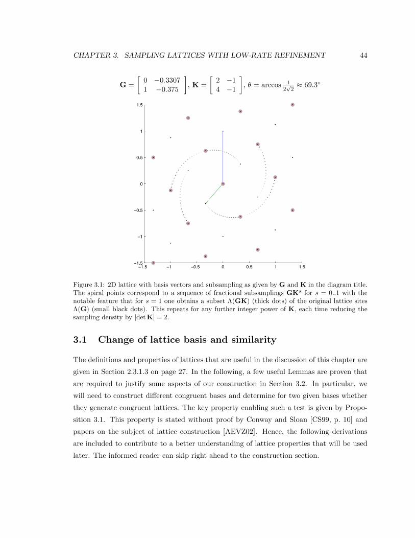
CHAPTER 3. SAMPLING LATTICES WITH LOW-RATE REFINEMENT 44
G =
[0 −0.33071 −0.375
], K =
[2 −14 −1
], θ = arccos 1
2√
2≈ 69.3
−1.5 −1 −0.5 0 0.5 1 1.5−1.5
−1
−0.5
0
0.5
1
1.5
Figure 3.1: 2D lattice with basis vectors and subsampling as given by G and K in the diagram title.The spiral points correspond to a sequence of fractional subsamplings GKs for s = 0..1 with thenotable feature that for s = 1 one obtains a subset Λ(GK) (thick dots) of the original lattice sitesΛ(G) (small black dots). This repeats for any further integer power of K, each time reducing thesampling density by |det K| = 2.
3.1 Change of lattice basis and similarity
The definitions and properties of lattices that are useful in the discussion of this chapter are
given in Section 2.3.1.3 on page 27. In the following, a few useful Lemmas are proven that
are required to justify some aspects of our construction in Section 3.2. In particular, we
will need to construct different congruent bases and determine for two given bases whether
they generate congruent lattices. The key property enabling such a test is given by Propo-
sition 3.1. This property is stated without proof by Conway and Sloan [CS99, p. 10] and
papers on the subject of lattice construction [AEVZ02]. Hence, the following derivations
are included to contribute to a better understanding of lattice properties that will be used
later. The informed reader can skip right ahead to the construction section.
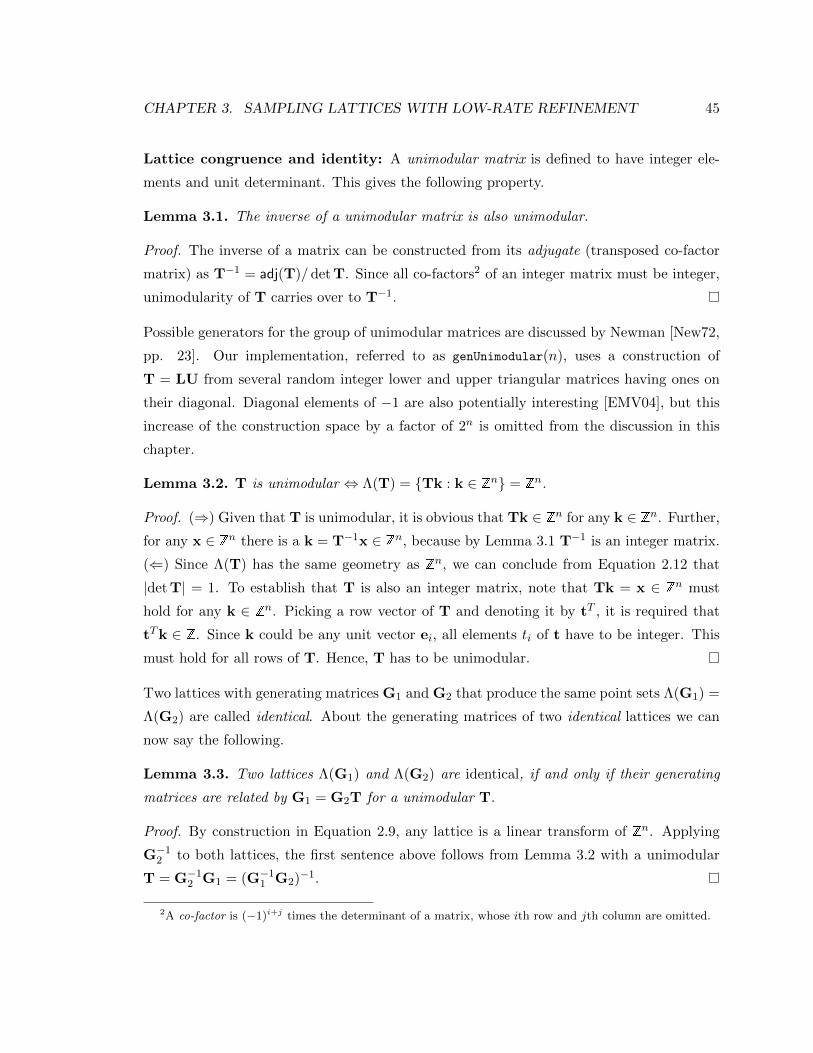
CHAPTER 3. SAMPLING LATTICES WITH LOW-RATE REFINEMENT 45
Lattice congruence and identity: A unimodular matrix is defined to have integer ele-
ments and unit determinant. This gives the following property.
Lemma 3.1. The inverse of a unimodular matrix is also unimodular.
Proof. The inverse of a matrix can be constructed from its adjugate (transposed co-factor
matrix) as T−1 = adj(T)/ det T. Since all co-factors2 of an integer matrix must be integer,
unimodularity of T carries over to T−1.
Possible generators for the group of unimodular matrices are discussed by Newman [New72,
pp. 23]. Our implementation, referred to as genUnimodular(n), uses a construction of
T = LU from several random integer lower and upper triangular matrices having ones on
their diagonal. Diagonal elements of −1 are also potentially interesting [EMV04], but this
increase of the construction space by a factor of 2n is omitted from the discussion in this
chapter.
Lemma 3.2. T is unimodular ⇔ Λ(T) = Tk : k ∈ Zn = Zn.
Proof. (⇒) Given that T is unimodular, it is obvious that Tk ∈ Zn for any k ∈ Zn. Further,
for any x ∈ Zn there is a k = T−1x ∈ Zn, because by Lemma 3.1 T−1 is an integer matrix.
(⇐) Since Λ(T) has the same geometry as Zn, we can conclude from Equation 2.12 that
|det T| = 1. To establish that T is also an integer matrix, note that Tk = x ∈ Zn must
hold for any k ∈ Zn. Picking a row vector of T and denoting it by tT , it is required that
tTk ∈ Z. Since k could be any unit vector ei, all elements ti of t have to be integer. This
must hold for all rows of T. Hence, T has to be unimodular.
Two lattices with generating matrices G1 and G2 that produce the same point sets Λ(G1) =
Λ(G2) are called identical. About the generating matrices of two identical lattices we can
now say the following.
Lemma 3.3. Two lattices Λ(G1) and Λ(G2) are identical, if and only if their generating
matrices are related by G1 = G2T for a unimodular T.
Proof. By construction in Equation 2.9, any lattice is a linear transform of Zn. Applying
G−12 to both lattices, the first sentence above follows from Lemma 3.2 with a unimodular
T = G−12 G1 = (G−1
1 G2)−1.
2A co-factor is (−1)i+j times the determinant of a matrix, whose ith row and jth column are omitted.

CHAPTER 3. SAMPLING LATTICES WITH LOW-RATE REFINEMENT 46
An immediate consequence of this is the following statement by Conway and Sloane [CS99,
p. 10, Eq. 23].
Proposition 3.1. The Gram matrices of two congruent lattices are related via A1 =
TTA2T for some unimodular T.
Proof. By Equation 2.10 and Lemma 3.3 we have A1 = GT1 G1 = TTGT
2 G2T = TTA2T.
The matrix T manipulates each column vector of G by adding integer multiples of other
column vectors. While not changing the position of the points in the lattice, this transfor-
mation does affect their integer coordinates (multi-indices).
Reduction: A good reason to search for a particular unimodular transformation T is to
obtain a reduced basis for a given lattice. Here, the objective is to choose equivalent basis
vectors such that the indices k of the Voronoi relevant neighbourhood (Equation 2.7 on
page 25) around the origin are contained within a small radius. This is a rough outline of the
different formal reduction criteria by Hermite, Minkowski, and others [AEVZ02, ZAM08].
Equivalence check: Even for triangular generating matrices scaled to unit determinant, a
check for equivalence of two generating matrices is an NP-complete problem [vEB81, GJ79].
An equivalent test can be done by extracting and comparing the Voronoi polytopes of two
lattices, which fall into the same complexity class.
Our method employs a simpler necessary test for equivalence by looking at the first few
elements of the set q(A) = kTAk : k ∈ Zn using the Gram matrix A of a reduced lattice
basis scaled to unit determinant. If the sorted lists q(A1) and q(A2) of two lattices disagree
in any element, G1 and G2 are not equivalent (also suggested by Newman [New72, p. 60]).
Equivalently, it is possible to restrict the list for this test to the Voronoi relevant indices
K = G−1N(0) of Equation 2.7 instead of all k ∈ Zn.
Dilation: Regular subsampling of a lattice can be expressed via a dilation matrix K ∈ Zn×n
to form a new lattice with generating matrix GK. The rate of reduction in sampling density
corresponds to
|det K| = αn = β ∈ Z+, (3.1)
which is the factor that scales the volume of the fundamental parallelepiped (Equation 2.12).
In the context of wavelet and multi-channel filter bank design Kovacevic and Vetterli [KV92]
define conditions for admissible sub-sampling matrices K:
CHAPTER 3. SAMPLING LATTICES WITH LOW-RATE REFINEMENT 47
• Λ(GK) ⊂ Λ(G),
• the eigenvalues λi of K must satisfy |λi| > 1, and
• ideally, all |λi| = α to preserve the directional geometry of the signal.
The last property ensures that that the subsampled signal is treated equally in all basis
directions. Only few iterations of sub-sampling should produce the same type of lattice that
the construction starts from, i.e. for a small number c of iterations one would like Kc = αcI
for αc ∈ Z.
Dyadic subsampling with K = 2I discards every second sample along each of the n
dimensions resulting in a reduction rate of β = 2n that grows exponentially in n. Entezari
et al. [EMV04] construct an admissible dilation with a smaller reduction rate for the body
centered cubic (BCC) lattice giving β = 4 and c = 3 in n = 3.
Van De Ville et al. [VDVBU05b] consider the 2D quincunx subsampling, which is an
interesting case permitting a two-channel dilation (β = 2) in n = 2. With the implicit
assumption of starting from the Cartesian lattice they show that dilations with β = 2 do
not exist for n > 2.
The main idea of the following construction is to relax the starting condition to include
general generators G ∈ Rn. It is then shown that a dimensionally independent low-rate
dilation becomes possible for any n. To allow for fine-grained scale progression we are
particularly interested in low subsampling rates, such as β = 2 or 3 that are not affected by
the dimensionality n. This means that point distances change by a factor as low as α = 21/n.
3.2 Construction of sampling lattices with low-rate rotational
dilation
We are looking for a non-singular lattice generating matrix G that, when sub-sampled by a
dilation matrix K with reduction rate β as in Equation 3.1, produces a similar lattice, that
is, it can be scaled and rotated by a matrix Q with QTQ = α2I. These are formal properties
behind the example given earlier in Figure 3.1. Algebraically, such an equivalence between
Λ(G) and the dilated Λ(GK) can be expressed as
QG = GK, (3.2)
CHAPTER 3. SAMPLING LATTICES WITH LOW-RATE REFINEMENT 48
leading to the observation that dilation K and scaled rotation Q are related by a similarity
transform
G−1QG = K. (3.3)
Suitable K for equivalent dilation: Using a matrix J2 =
[1 j
1 −j
]it is possible to
diagonalize a rotation matrix in R2×2 by the following similarity transform
1
αQ2 =
[cos θ − sin θ
sin θ cos θ
]= J−1
2
[ejθ 0
0 e−jθ
]J2 = J−1
2 ∆J2, (3.4)
where ∆ contains a pair of complex conjugate eigenvalues. Substituting this decomposition
for Q in Equation 3.2 leads to
K = αG−1J−1n ∆JnG, (3.5)
K = αP∆P−1, (3.6)
where the first equation gives the structure of K and the second one its eigendecomposition,
which can be computed. Putting this together allows to obtain lattice basis and rotation as
G = J−1n P−1
Q = αJ−1n ∆Jn.
(3.7)
Thus, given a matrix K that has an eigendecomposition corresponding to that of a uni-
formly scaled rotation matrix Q, we can compute the lattice generating matrix G as in
Equation 3.7. To allow for later optimization, it would be nice to be able to generate more
than one or, ideally, all possible solutions to this construction. The non-unicity of the eigen-
decomposition allows to insert an additional diagonal matrix S that scales the otherwise
unit eigenvectors in the columns of P
K = αG−1J−1n S∆S−1JnG (3.8)
again using Equation 3.6 gives a different G for the same rotation Q as
G = J−1n SP−1. (3.9)

CHAPTER 3. SAMPLING LATTICES WITH LOW-RATE REFINEMENT 49
The resulting G may be complex valued. Turning it into a real matrix by taking its real or
imaginary components does, however, not destroy the similarity relationship of Equation 3.3.
With G normalized to unit determinant this basis vector scaling introduces n−1 additional
degrees of freedom into the design. Below, we will refer to this construction as function
formGQ(K,S) using S = I by default.
3.2.1 Constructing rotational dilation matrices
The following proposition is key to the construction of integer K that facillitate the rota-
tional dilation of Equation 3.2.
Proposition 3.2. The similarity of K with a rotation matrix Q (Equation 3.3) and its
diagonalization α∆ (Equation 3.4) imposes restrictions on the coefficients ck of their shared
characteristic polynomial
dK(λ) = det(K− λI) =n∑k=0
ckλk, (3.10)
where dK(λ) = dQ(λ) = d∆(λ/α) with α as given in Equation 3.1 and β being a simple
product of primes.
For even n: the only non-zero integer coefficients are c0 = β, c2n/2 < 4β, cn = 1. This
leaves a finite number of options for cn/2.
For odd n: a single polynomial d(λ) is possible with non-zero coefficients c0 = −β, cn = 1.
The proof is given in Section 3.2.2.
Finding all possible integer K that fulfill Proposition 3.2 is a hard problem to which we
have not yet found a complete solution. Our initial approach used an exhaustive search,
which is possible for all integer elements within certain bounds. For n = 2 and β = 2 this
gave all three cases shown later in the results.
However, the following observation enables a direct construction for any n. The con-
straints in Proposition 3.2 prescribe monic polynomials with cn = 1. This makes it possible
CHAPTER 3. SAMPLING LATTICES WITH LOW-RATE REFINEMENT 50
to directly construct a suitable K via the companion matrix [TI97, p. 192]
K =
0 −c0
1 0 −c1
1 0...
. . .. . . −cn−2
1 −cn−1
. (3.11)
that fulfills Equation 3.3. We refer to the above procedure as function compoly(n, α, cn/2)
that returns a companion matrix (Equation 3.11) with a characteristic polynomial as in
Equation 3.15 or 3.18.
Obtaining alternative dilation matrices: With this starting point it is possible to
construct additional suitable dilation matrices via a similarity transform with a unimodular
matrix T
KT = TKT−1 = PT∆P−1T . (3.12)
By Lemma 3.1 KT remains an integer matrix. By Equation 3.5 and Equation 3.7 a call
to formGQ(KT ) leads to a new basis GT = GT that by Lemma 3.3 generates an identical
lattice. So, this method can not be used to search for new lattices, but allows to perform a
reduction of G as explained in Section 3.1.
Optimizing further non-equivalent solutions: The introduction of diagonal eigenvector
scaling S in Equation 3.7 as a second parameter to formGQ allows to construct non-equivalent
lattice bases G and introduces n−1 degrees of freedom into the construction. In this search
space it is possible to optimize further criteria, such as the ones discussed in Section 2.3.1.2
and Section 2.3.3 to select the “best” lattice.
3.2.2 Characteristic polynomial of a scaled rotation matrix in Rn
The similarity relationship between K and Q in Equation 3.2 implies that they share the
same characteristic polynomial d(λ) of Equation 3.10. First, note that the zero crossings of
d(λ) determine the eigenvalues d(λk) = 0 and determinant β = d(0) = c0 fixes the constant
of the polynomial [TI97, p. 184]. Further, since K is an integer matrix the polynomial
d(λ) ∈ Z[λ] has integer coefficients ck.
In order to find integer matrices K with the eigenvalues of a scaled rotation matrix,
CHAPTER 3. SAMPLING LATTICES WITH LOW-RATE REFINEMENT 51
it will be important to distinguish the two different forms of the diagonal matrix ∆ in
Equation 3.4, 3.5, and 3.8 for the case of even n
∆ = diag[ejθ1 e−jθ1 . . . ejθn/2 e−jθn/2 ]
and the case of odd n
∆ = diag[1 ejθ1 e−jθ1 . . . ejθ(n−1)/2 e−jθ(n−1)/2 ]
with analogue block-wise constructions to form Jn from J2 of Equation 3.4.
The following proof of Proposition 3.2 is due to a collaboration with Thierry Blu.
Proof. For even dimensionality n the characteristic polynomial of K and Q fulfills
d(λ) =
n/2∏k=1
(αejθk − λ)(αe−jθk − λ)
=
n/2∏k=1
(α2 − 2λα cos θk + λ2)
=
n/2∏k=1
[(α4
λ2− 2
α3
λcos θk + α2
)λ2
α2
]= d
(α2
λ
)(λ
α
)n.
(3.13)
Thus, if
d(λ) =n∑k=0
ckλk
=
n∑k=0
ck
(α2
λ
)k (λ
α
)n=
n∑k=0
cn−kαn−2kλk
⇔ ck = αn−2kcn−k = β1− 2kn cn−k.
(3.14)
If ck 6= 0 and ck, β ∈ Z then β1− 2kn ∈ Q. This is impossible for 0 < 2k < n, assuming small
values of β, such as 2, 3 or any simple product of primes. This implies that ck = cn−k = 0
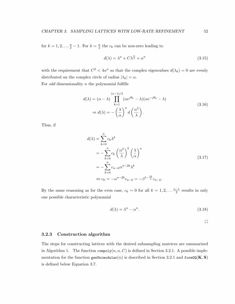
CHAPTER 3. SAMPLING LATTICES WITH LOW-RATE REFINEMENT 52
for k = 1, 2, . . . n2 − 1. For k = n2 the ck can be non-zero leading to
d(λ) = λn + Cλn2 + αn (3.15)
with the requirement that C2 < 4αn so that the complex eigenvalues d(λk) = 0 are evenly
distributed on the complex circle of radius |λk| = α.
For odd dimensionality n the polynomial fulfills
d(λ) = (α− λ)
(n−1)/2∏k=1
(αejθk − λ)(αe−jθk − λ)
⇒ d(λ) = −(λ
α
)nd
(α2
λ
).
(3.16)
Thus, if
d(λ) =n∑k=0
ckλk
= −n∑k=0
ck
(α2
λ
)k (λ
α
)n= −
n∑k=0
cn−kαn−2kλk
⇔ ck = −αn−2kcn−k = −β1− 2kn cn−k.
(3.17)
By the same reasoning as for the even case, ck = 0 for all k = 1, 2, . . . n−12 results in only
one possible characteristic polynomial
d(λ) = λn − αn. (3.18)
3.2.3 Construction algorithm
The steps for constructing lattices with the desired subsampling matrices are summarized
in Algorithm 1. The function compoly(n, α,C) is defined in Section 3.2.1. A possible imple-
mentation for the function genUnimodular(n) is described in Section 3.2.1 and formGQ(K,S)
is defined below Equation 3.7.
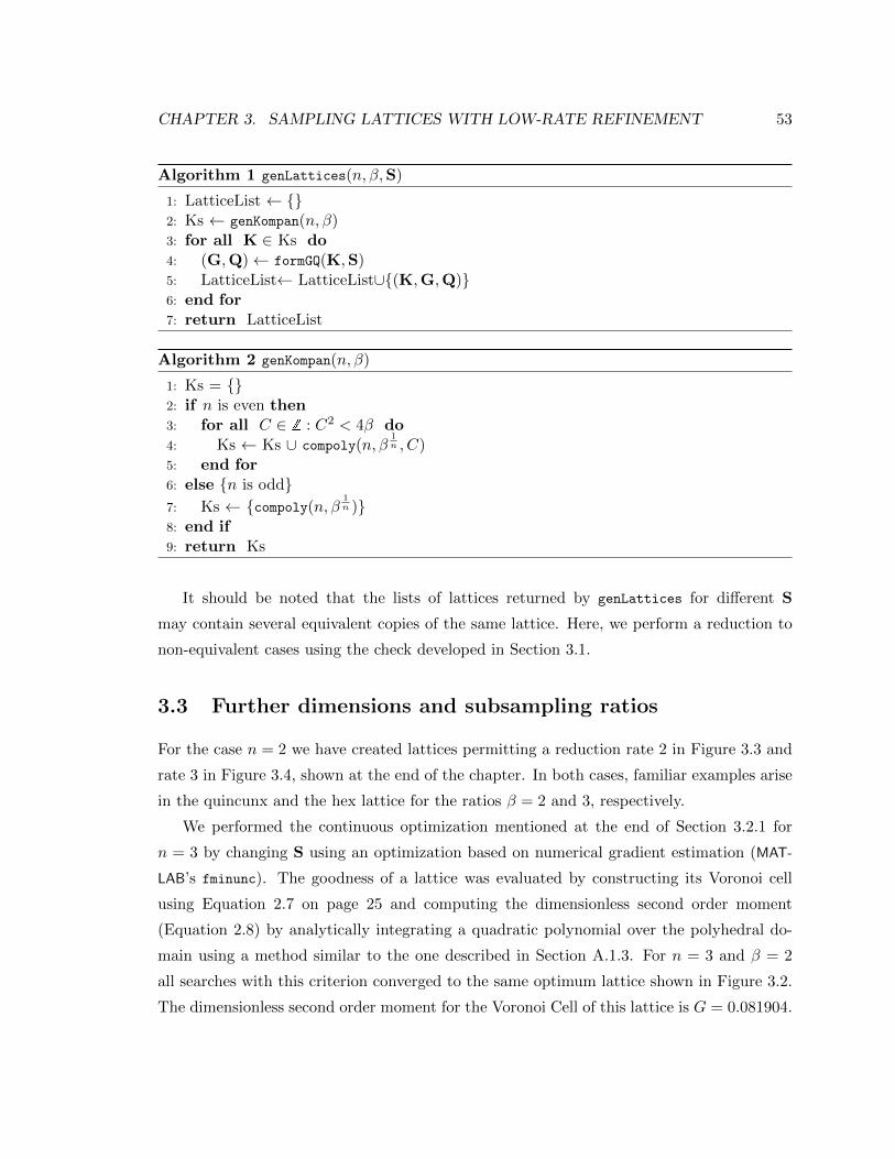
CHAPTER 3. SAMPLING LATTICES WITH LOW-RATE REFINEMENT 53
Algorithm 1 genLattices(n, β,S)
1: LatticeList ← 2: Ks ← genKompan(n, β)3: for all K ∈ Ks do4: (G,Q)← formGQ(K,S)5: LatticeList← LatticeList∪(K,G,Q)6: end for7: return LatticeList
Algorithm 2 genKompan(n, β)
1: Ks = 2: if n is even then3: for all C ∈ Z : C2 < 4β do4: Ks ← Ks ∪ compoly(n, β
1n , C)
5: end for6: else n is odd7: Ks ← compoly(n, β
1n )
8: end if9: return Ks
It should be noted that the lists of lattices returned by genLattices for different S
may contain several equivalent copies of the same lattice. Here, we perform a reduction to
non-equivalent cases using the check developed in Section 3.1.
3.3 Further dimensions and subsampling ratios
For the case n = 2 we have created lattices permitting a reduction rate 2 in Figure 3.3 and
rate 3 in Figure 3.4, shown at the end of the chapter. In both cases, familiar examples arise
in the quincunx and the hex lattice for the ratios β = 2 and 3, respectively.
We performed the continuous optimization mentioned at the end of Section 3.2.1 for
n = 3 by changing S using an optimization based on numerical gradient estimation (MAT-
LAB’s fminunc). The goodness of a lattice was evaluated by constructing its Voronoi cell
using Equation 2.7 on page 25 and computing the dimensionless second order moment
(Equation 2.8) by analytically integrating a quadratic polynomial over the polyhedral do-
main using a method similar to the one described in Section A.1.3. For n = 3 and β = 2
all searches with this criterion converged to the same optimum lattice shown in Figure 3.2.
The dimensionless second order moment for the Voronoi Cell of this lattice is G = 0.081904.
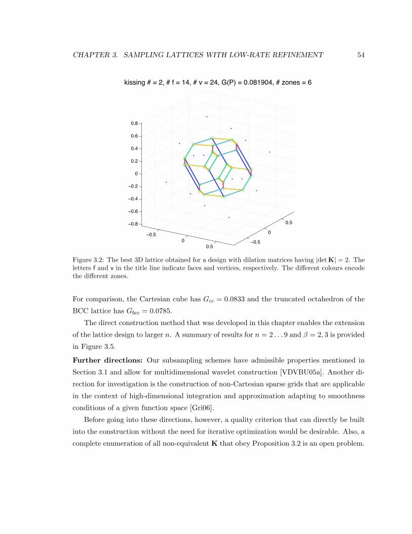
CHAPTER 3. SAMPLING LATTICES WITH LOW-RATE REFINEMENT 54
−0.50
0.5−0.5
0
0.5−0.8
−0.6
−0.4
−0.2
0
0.2
0.4
0.6
0.8
kissing # = 2, # f = 14, # v = 24, G(P) = 0.081904, # zones = 6
Figure 3.2: The best 3D lattice obtained for a design with dilation matrices having |det K| = 2. Theletters f and v in the title line indicate faces and vertices, respectively. The different colours encodethe different zones.
For comparison, the Cartesian cube has Gcc = 0.0833 and the truncated octahedron of the
BCC lattice has Gbcc = 0.0785.
The direct construction method that was developed in this chapter enables the extension
of the lattice design to larger n. A summary of results for n = 2 . . . 9 and β = 2, 3 is provided
in Figure 3.5.
Further directions: Our subsampling schemes have admissible properties mentioned in
Section 3.1 and allow for multidimensional wavelet construction [VDVBU05a]. Another di-
rection for investigation is the construction of non-Cartesian sparse grids that are applicable
in the context of high-dimensional integration and approximation adapting to smoothness
conditions of a given function space [Gri06].
Before going into these directions, however, a quality criterion that can directly be built
into the construction without the need for iterative optimization would be desirable. Also, a
complete enumeration of all non-equivalent K that obey Proposition 3.2 is an open problem.
CHAPTER 3. SAMPLING LATTICES WITH LOW-RATE REFINEMENT 55
quincunx, θ = 45 θ = arccos√
22 ≈ 69.3 θ = 135
G =
[ √2 0
0√2
], K =
[−1 −11 −1
]G =
[0 0.61
−0.93 −0.23
], K =
[−1 −12 0
]G =
[0 0.58
−1.22 0.41
], K =
[1 −13 −1
]
2 1 0 1 22
1.5
1
0.5
0
0.5
1
1.5
2
2 1 0 1 22
1.5
1
0.5
0
0.5
1
1.5
2
2 1 0 1 22
1.5
1
0.5
0
0.5
1
1.5
2
4 2 0 2 44
3
2
1
0
1
2
3
4
4 2 0 2 44
3
2
1
0
1
2
3
4
4 2 0 2 44
3
2
1
0
1
2
3
4
Figure 3.3: Three non-equivalent 2D lattices obtained for a design with dilation matrices having|det K| = 2. The lattice in the first column is the known quincunx sampling with a rotation ofθ = 45. The other two are new schemes with different rotation angles. The thick dots show thesample positions that are retained after subsampling by K. The second row shows the same latticeat twice the density, with more iteration levels of similarity transformed Voronoi cells.
0 50
1
2
3
4
5
1: R = [−0 0.93;1.1 −0.54] K = [−1 2;−2 1] θ=90
0 50
1
2
3
4
5
2: R = [0 0.84;−1.2 0] K = [1 −1;2 1] θ=54.74
0 50
1
2
3
4
5
3: R = [0 0.74;−1.3 0.22] K = [1 −1;3 0] θ=73.22
0 50
1
2
3
4
5
4: R = [0.66 0;1.1 −1.5] K = [−3 4;−3 3] θ=90
Figure 3.4: Four non-equivalent 2D lattices obtained for a design with dilation matrices having|det K| = 3. The lattice on the left is the well known hexagonal lattice with a θ = 30 rotation. Theother three are new schemes with different rotation angles.

CHAPTER 3. SAMPLING LATTICES WITH LOW-RATE REFINEMENT 56
1 2 3 4 5 6 7 8 9
0.35
0.4
0.45
0.5
0.55
0.6
0.65
0.7
0.75
0.8
0.85
Packing radii
ρ=δ1/n
Cartesiandensest known latticesupper bound r
n
β=2−optimizedβ=3−optimizedβ=2−companionβ=3−companion
n
Figure 3.5: Comparison of packing radii of best known packings, Cartesian packing, and the upperbound as in Figure 2.3 on page 33. In addition, some designs of this chapter are shown that enjoy thelow-rate rotational reduction property of Equation 3.2 for rates β ∈ 2, 3. If proceeding directly froma companion K as provided by Algorithm 2 unoptimized constructions can be generated instantlyfor any n. The optimized designs are obtained by maximization of the packing radius over choicesof S in Equation 3.9. The depicted results beat Cartesian packing in all cases except for n ∈ 1, 3.

Chapter 4
A sampling bound for composed functions
A fundamental problem in image synthesis is the evaluation of the rendering integral [PH04c].
In particular, volume rendering is based on a version that requires a mapping of given data
values f(x) to optical properties. By slightly abstracting the integrand within the volume
rendering integral, this mapping can be viewed as a composite function g(f(x)) = h(x),
where g is the mapping that assigns optical properties (i.e. opacities) to values of the data
f . In the context of volume graphics g is referred to as a transfer function. The actual input
to the rendering algorithm is the signal g(f(x)) = (g f)(x). Besides the chosen quadrature
formula for evaluating the integral, a crucial parameter determining the accuracy of the
numerical solution to the integral is the sampling distance. Since it is common to use linear
interpolation, it is important to use at least twice the Nyquist rate in order to guarantee an
accurate evaluation of the integral.
Despite the common use of this approach of sampling a composed data function it has
not yet undergone a satisfactory mathematical analysis. In particular, there were no clear
statements on how the mapped function is to be sampled appropriately. The only known
exception was the previous work [EKE01b, Kra03, SKLE03], which suggests that the proper
essential Nyquist rate of (gf) is proportional to the product of the respective Nyquist rates.
However, this estimate is too restricted for many data models and is mostly over-estimating,
as demonstrated in Figure 4.1. The knowledge of the proper sampling rate of the function
(g f)(x) will enable us to not only predict a proper error behaviour, but allows us to
accelerate rendering algorithms by skipping over regions that need less sampling in order
to guarantee a particular error behavior. While fast, high-quality solutions for quantized 8-
bit data exist in form of pre-integrated transfer functions, adequate sampling rates for high
57

CHAPTER 4. A SAMPLING BOUND FOR COMPOSED FUNCTIONS 58
−3 −2 −1 0 1 2 30
0.5
1
x
(a) Example data signal:f(x) = 0.5 + 9
20sin( 2π
4x) + 1
20sin(4πx)
0 0.2 0.4 0.6 0.8 1
0
0.5
1
y
(b) A transfer function: g(y) = 12(1− cos(2πy))
−3 −2 −1 0 1 2 3
0
0.5
1
x
(c) Sampling g(f(x)) at 4 times the boundingfrequency π
2νgωh
−3 −2 −1 0 1 2 3
0
0.5
1
x
(d) Sampling g(f(x)) at 4 times the boundingfrequency νg max |f ′|
Figure 4.1: Sampling comparison. The data y = f(x) (a) is composed with a transfer functiong(y) (b). Figures (c) and (d) show sinc-interpolated samplings of g(f(x)). The tighter boundingfrequency (d) suggested in this chapter results in 5 times fewer samples for these particular f andg, still truthfully representing the composite signal.
dynamic range volumes and multi-modal or multi-dimensional data, such as (f, |f ′|), are yet
unknown. Typical estimates are based on a proper sampling of f alone, which neglects the
effect of the transfer function. In the following we present an estimate for suitable sampling
that takes the effect of the transfer function into account.
For that purpose, we investigate [BMWM06] the effects of function composition in the
form g(f(x)) = h(x) by means of a spectral analysis of h.1 Building on related work
discussed in Section 2.4.3, in Section 4.1 we provide a rigorous mathematical treatment that
decomposes the spectral description of h into a scalar product of the spectral description of
g and a term that solely depends on f and that is independent of g. We then use the method
of stationary phase to derive the essential maximum frequency of g(f(x)) bounding the main
portion of the energy of its spectrum. This limit is the product of the maximum frequency of
g and the maximum derivative of f . This leads to a proper sampling of the composition h of
the two functions g and f . We apply our theoretical results to a fundamental open problem
in volume rendering—the proper sampling of the rendering integral after the application of
a transfer function. In particular, Section 4.2 demonstrates how the sampling criterion can
1Note that the order of f and h is exchanged from the abstraction in Section 1.4. Also, interactiveparameter space exploration does not apply in this chapter.
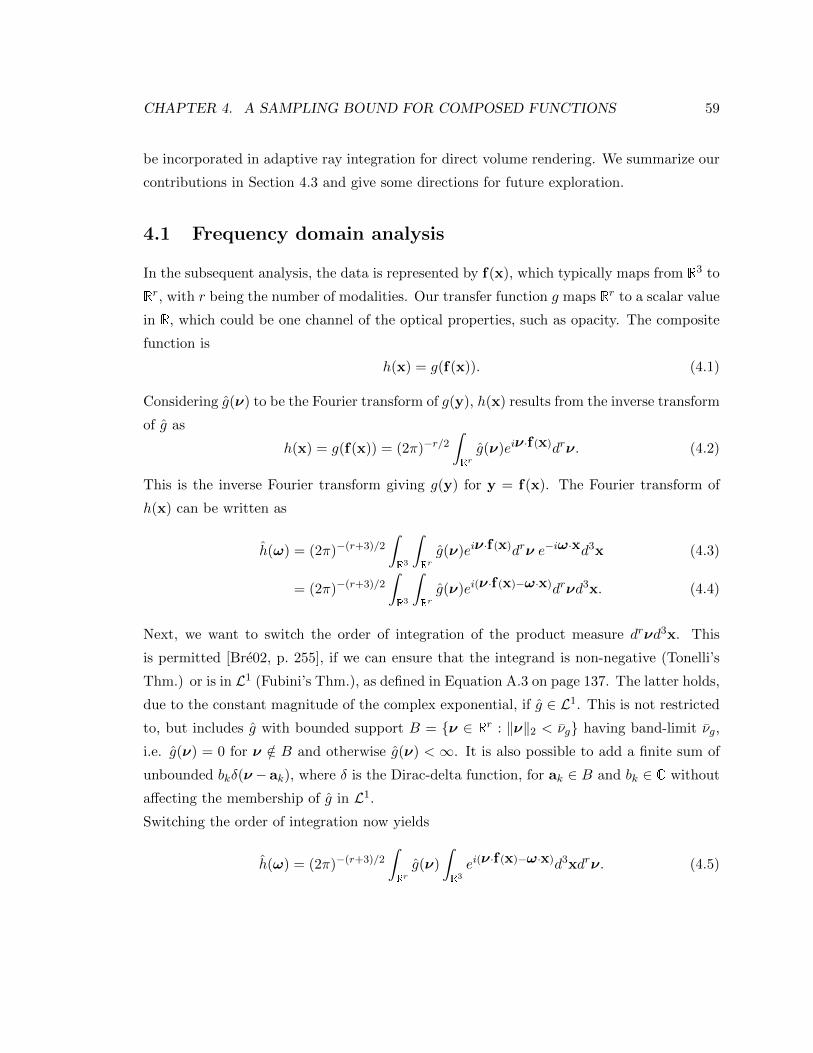
CHAPTER 4. A SAMPLING BOUND FOR COMPOSED FUNCTIONS 59
be incorporated in adaptive ray integration for direct volume rendering. We summarize our
contributions in Section 4.3 and give some directions for future exploration.
4.1 Frequency domain analysis
In the subsequent analysis, the data is represented by f(x), which typically maps from R3 to
Rr, with r being the number of modalities. Our transfer function g maps Rr to a scalar value
in R, which could be one channel of the optical properties, such as opacity. The composite
function is
h(x) = g(f(x)). (4.1)
Considering g(ν) to be the Fourier transform of g(y), h(x) results from the inverse transform
of g as
h(x) = g(f(x)) = (2π)−r/2∫Rr
g(ν)eiν ·f (x)drν. (4.2)
This is the inverse Fourier transform giving g(y) for y = f(x). The Fourier transform of
h(x) can be written as
h(ω) = (2π)−(r+3)/2
∫R3
∫Rr
g(ν)eiν ·f (x)drν e−iω·xd3x (4.3)
= (2π)−(r+3)/2
∫R3
∫Rr
g(ν)ei(ν ·f (x)−ω·x)drνd3x. (4.4)
Next, we want to switch the order of integration of the product measure drνd3x. This
is permitted [Bre02, p. 255], if we can ensure that the integrand is non-negative (Tonelli’s
Thm.) or is in L1 (Fubini’s Thm.), as defined in Equation A.3 on page 137. The latter holds,
due to the constant magnitude of the complex exponential, if g ∈ L1. This is not restricted
to, but includes g with bounded support B = ν ∈ Rr : ‖ν‖2 < νg having band-limit νg,
i.e. g(ν) = 0 for ν /∈ B and otherwise g(ν) < ∞. It is also possible to add a finite sum of
unbounded bkδ(ν − ak), where δ is the Dirac-delta function, for ak ∈ B and bk ∈ C without
affecting the membership of g in L1.
Switching the order of integration now yields
h(ω) = (2π)−(r+3)/2
∫Rr
g(ν)
∫R3
ei(ν ·f (x)−ω·x)d3xdrν. (4.5)

CHAPTER 4. A SAMPLING BOUND FOR COMPOSED FUNCTIONS 60
Noticing that the inner integral is independent of g, we use
K(ω,ν) =
∫R3
(2π)−(r+3)/2ei(ν ·f (x)−ω·x)d3x to write more concisely (4.6)
h(ω) =
∫Rr
g(ν)K(ω,ν)drν (4.7)
= 〈g∗(·), K(ω, ·)〉ν . (4.8)
This shows that forming the frequency spectrum h(ω) of the composition g f can be
interpreted as application of a linear operator with kernel K to the spectrum g(ν), which
can be implemented by means of a dot product with the complex conjugate of g for each
target frequency ω, as defined in Equation A.4. In the following, we will take a closer look
at the properties of the frequency transfer kernel K(ω,ν).
4.1.1 Visual inspection of the frequency transfer kernel K(ω,ν)
The kernel K(ω,ν) of Equation 4.6 solely depends on properties of f and is independent of
the mapping g. Further, in its role as a kernel of the linear operator used in Equation 4.8 it
can be interpreted as a map that determines how much of the energy of a certain frequency
component ν of g is mapped to a frequency ω in the target spectrum h.
To get an intuition for the properties of this function we will first inspect it visually.
Figure 4.2 shows K(ω, ν) for different one-dimensional scalar functions f(x), which is why
the bold notation is dropped at this point. In particular we have chosen a single Gaussian
function and a combination of two Gaussian functions. K(ω, ν) is computed as the discrete
Fourier transform of eiνf(x), which is a possible interpretation of a distretized Equation 4.6.
The picture has to be imagined periodically continued in ω (horizontally), which is due to
the discrete computation. In fact, the bright lines cutting off the corners in Figure 4.2d
are due to that effect. This does not apply to the continuous case that we deal with in the
subsequent analysis. Further, the function is point symmetric, or more precisely Hermitian,
since from Equation 4.6 it follows that K(ω, ν) = K∗(−ω,−ν).
A significant property apparent from Figure 4.2 is the low-valued cone in the middle,
starting narrow at ν = ω = 0 and increasing in size towards larger ω. According to
Equation 4.8 the spectrum of the composite function h(ω) is formed by the dot product
with the conjugate spectrum g∗(ν). In order to determine at which maximum wavenumber
ω = ωh the function h(ω) ceases to have a significant contribution, we have to figure out
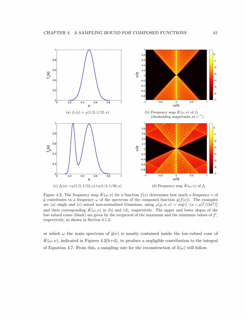
CHAPTER 4. A SAMPLING BOUND FOR COMPOSED FUNCTIONS 61
0 0.2 0.4 0.6 0.8 10
0.2
0.4
0.6
0.8
1f 1(x)
x
(a) f1(x) = ϕ(1/2, 1/12, x)
!/"
#/"
−1 −0.5 0 0.5 1
−0.8
−0.6
−0.4
−0.2
0
0.2
0.4
0.6
0.8
1
−7
−6
−5
−4
−3
−2
−1
0
(b) Frequency map K(ω, ν) of f1(thesholding magnitudes at e−7)
0 0.2 0.4 0.6 0.8 10
0.2
0.4
0.6
0.8
1
f 2(x)
x(c) f2(x) =ϕ(1/2, 1/12, x)+ϕ(1/4, 1/30, x)
!/"
#/"
−1 −0.5 0 0.5 1
−0.8
−0.6
−0.4
−0.2
0
0.2
0.4
0.6
0.8
1
−7
−6
−5
−4
−3
−2
−1
0
(d) Frequency map K(ω, ν) of f2
Figure 4.2: The frequency map K(ω, ν) for a function f(x) determines how much a frequency ν ofg contributes to a frequency ω of the spectrum of the composed function g(f(x)). The examplesare (a) single and (c) mixed non-normalized Gaussians, using ϕ(µ, σ, x) = exp
(−(x− µ)2/(2σ2)
)and their corresponding K(ω, ν) in (b) and (d), respectively. The upper and lower slopes of thelow-valued cones (black) are given by the reciprocal of the maximum and the minimum values of f ′,respectively, as shown in Section 4.1.2.
at which ω the main spectrum of g(ν) is mostly contained inside the low-valued cone of
K(ω, ν), indicated in Figures 4.2(b+d), to produce a negligible contribution to the integral
of Equation 4.7. From this, a sampling rate for the reconstruction of h(ω) will follow.
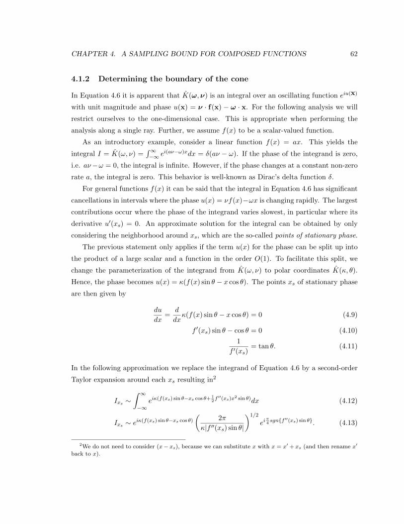
CHAPTER 4. A SAMPLING BOUND FOR COMPOSED FUNCTIONS 62
4.1.2 Determining the boundary of the cone
In Equation 4.6 it is apparent that K(ω,ν) is an integral over an oscillating function eiu(x)
with unit magnitude and phase u(x) = ν · f(x) − ω · x. For the following analysis we will
restrict ourselves to the one-dimensional case. This is appropriate when performing the
analysis along a single ray. Further, we assume f(x) to be a scalar-valued function.
As an introductory example, consider a linear function f(x) = ax. This yields the
integral I = K(ω, ν) =∫∞−∞ e
i(aν−ω)xdx = δ(aν − ω). If the phase of the integrand is zero,
i.e. aν−ω = 0, the integral is infinite. However, if the phase changes at a constant non-zero
rate a, the integral is zero. This behavior is well-known as Dirac’s delta function δ.
For general functions f(x) it can be said that the integral in Equation 4.6 has significant
cancellations in intervals where the phase u(x) = νf(x)−ωx is changing rapidly. The largest
contributions occur where the phase of the integrand varies slowest, in particular where its
derivative u′(xs) = 0. An approximate solution for the integral can be obtained by only
considering the neighborhood around xs, which are the so-called points of stationary phase.
The previous statement only applies if the term u(x) for the phase can be split up into
the product of a large scalar and a function in the order O(1). To facilitate this split, we
change the parameterization of the integrand from K(ω, ν) to polar coordinates K(κ, θ).
Hence, the phase becomes u(x) = κ(f(x) sin θ − x cos θ). The points xs of stationary phase
are then given by
du
dx=
d
dxκ(f(x) sin θ − x cos θ) = 0 (4.9)
f ′(xs) sin θ − cos θ = 0 (4.10)
1
f ′(xs)= tan θ. (4.11)
In the following approximation we replace the integrand of Equation 4.6 by a second-order
Taylor expansion around each xs resulting in2
Ixs ∼∫ ∞−∞
eiκ(f(xs) sin θ−xs cos θ+ 12f ′′(xs)x2 sin θ)dx (4.12)
Ixs ∼ eiκ(f(xs) sin θ−xs cos θ)
(2π
κ|f ′′(xs) sin θ|
)1/2
eiπ4sgnf ′′(xs) sin θ. (4.13)
2We do not need to consider (x− xs), because we can substitute x with x = x′ + xs (and then rename x′
back to x).

CHAPTER 4. A SAMPLING BOUND FOR COMPOSED FUNCTIONS 63
For f ′′(xs) considerably different from zero the integrand vanishes quickly as (x − xs)2
increases. The full integral is approximately obtained by summing all Ixs for all xs fulfilling
Equation 4.11. This case is relevant for points min(f ′) < 1tan θ < max(f ′). Outside this range
we do not have any points of stationary phase and the overall integral forming K(κ, θ) is
close to zero.
This observation establishes the main insight of our analysis: the extremal slopes of f
form the boundary of the cone observed in Figure 4.2. Therefore, the primary result of this
chapter is that the composite function has an essential maximum frequency of
ωh = νg maxx|f ′(x)| , (4.14)
where νg is the maximum frequency of g. The corresponding sampling rate should be chosen
just above the essential Nyquist rate of 2ωh.
Rapid decay at the boundary edge:3 An interesting case arises if one considers the
boundaries of the essentially band-limiting interval. They form the boundaries of the cone.
To inspect the range around this band edge we define a critical angle θe fulfilling tan θe =
1/f ′(xe) and f ′′(xe) = 0 with xe being a maximum point of f ′(x). Here, the second derivative
vanishes, which requires a third-order Taylor approximation of u(x). In the vicinity of the
band edge for θ h θe the resulting integral is
K(κ, θ) ∼∫ ∞−∞
exp[iκ(f(xe) sin θ − xe cos θ + (f ′(xe) sin θ − cos θ)x+1
6f ′′′(xe)x
3 sin θ)]dx
(4.15)
substituting x = αx using α =(
2κf ′′′(xe) sin θ
)1/3
K(κ, θ) ∼= eiκ(f(xe) sin θ−xe cos θ)α ·∫ ∞−∞
exp
[i
(κα(f ′(xe) sin θ − cos θ)x+
x3
3
)]dx (4.16)
3The discussion in this section is due to a collaboration with David J Muraki.
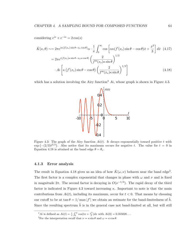
CHAPTER 4. A SAMPLING BOUND FOR COMPOSED FUNCTIONS 64
considering eis + e−is = 2 cos(s)
K(κ, θ) ∼= 2πeiκ(f(xe) sin θ−xe cos θ)α · 1
π
∫ ∞0
cos
[ακ(f ′(xe) sin θ − cos θ)x+
x3
3
]dx (4.17)
= 2πei(f(xe)κ sin θ−xeκ cos θ)
(2
f ′′′(xe)κ sin θ
)1/3
·Ai
[κ(f ′(xe) sin θ − cos θ
)( 2
f ′′′(xe)κ sin θ
)1/3]
(4.18)
which has a solution involving the Airy function4 Ai, whose graph is shown in Figure 4.3.
-5
0.4
0.2
0
-0.2
-0.4
1050-10
t
Ai(t)
Figure 4.3: The graph of the Airy function Ai(t). It decays exponentially toward positive t withexp
(−(2/3)t3/2
). Also notice that its maximum occurs for negative t. The value for t = 0 in
Equation 4.18 is attained at the band edge θ = θe.
4.1.3 Error analysis
The result in Equation 4.18 gives us an idea of how K(ω, ν) behaves near the band edge5.
The first factor is a complex exponential that changes in phase with ω and ν and is fixed
in magnitude 2π. The second factor is decaying in O(ν−1/3). The rapid decay of the third
factor is indicated in Figure 4.3 toward increasing κ. Important to note is that the main
contributions from Ai(t), including its maximum, occur for t < 0. That means by choosing
our cutoff to be at tan θ = 1/max |f ′| we obtain an estimate for the band-limitedness of h.
Since the resulting spectrum h is in the general case not band-limited at all, but will still
4Ai is defined as Ai(t) = 1π
∫∞0
cos(tx+ x3
3)dx with Ai(0) = 0.355028 . . .
5For the interpretation recall that ν = κ sin θ and ω = κ cos θ.
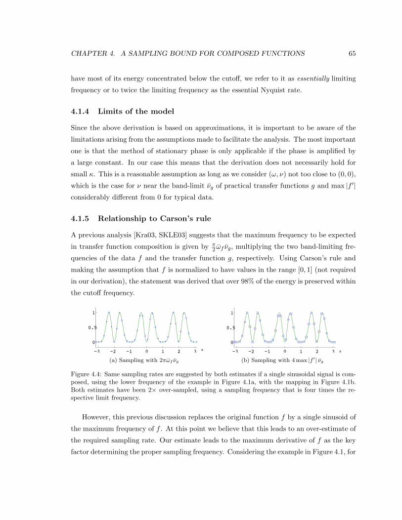
CHAPTER 4. A SAMPLING BOUND FOR COMPOSED FUNCTIONS 65
have most of its energy concentrated below the cutoff, we refer to it as essentially limiting
frequency or to twice the limiting frequency as the essential Nyquist rate.
4.1.4 Limits of the model
Since the above derivation is based on approximations, it is important to be aware of the
limitations arising from the assumptions made to facilitate the analysis. The most important
one is that the method of stationary phase is only applicable if the phase is amplified by
a large constant. In our case this means that the derivation does not necessarily hold for
small κ. This is a reasonable assumption as long as we consider (ω, ν) not too close to (0, 0),
which is the case for ν near the band-limit νg of practical transfer functions g and max |f ′|considerably different from 0 for typical data.
4.1.5 Relationship to Carson’s rule
A previous analysis [Kra03, SKLE03] suggests that the maximum frequency to be expected
in transfer function composition is given by π2 ωf νg, multiplying the two band-limiting fre-
quencies of the data f and the transfer function g, respectively. Using Carson’s rule and
making the assumption that f is normalized to have values in the range [0, 1] (not required
in our derivation), the statement was derived that over 98% of the energy is preserved within
the cutoff frequency.
−3 −2 −1 0 1 2 3
0
0.5
1
x
(a) Sampling with 2πωf νg
−3 −2 −1 0 1 2 3
0
0.5
1
x
(b) Sampling with 4 max |f ′| νg
Figure 4.4: Same sampling rates are suggested by both estimates if a single sinusoidal signal is com-posed, using the lower frequency of the example in Figure 4.1a, with the mapping in Figure 4.1b.Both estimates have been 2× over-sampled, using a sampling frequency that is four times the re-spective limit frequency.
However, this previous discussion replaces the original function f by a single sinusoid of
the maximum frequency of f . At this point we believe that this leads to an over-estimate of
the required sampling rate. Our estimate leads to the maximum derivative of f as the key
factor determining the proper sampling frequency. Considering the example in Figure 4.1, for
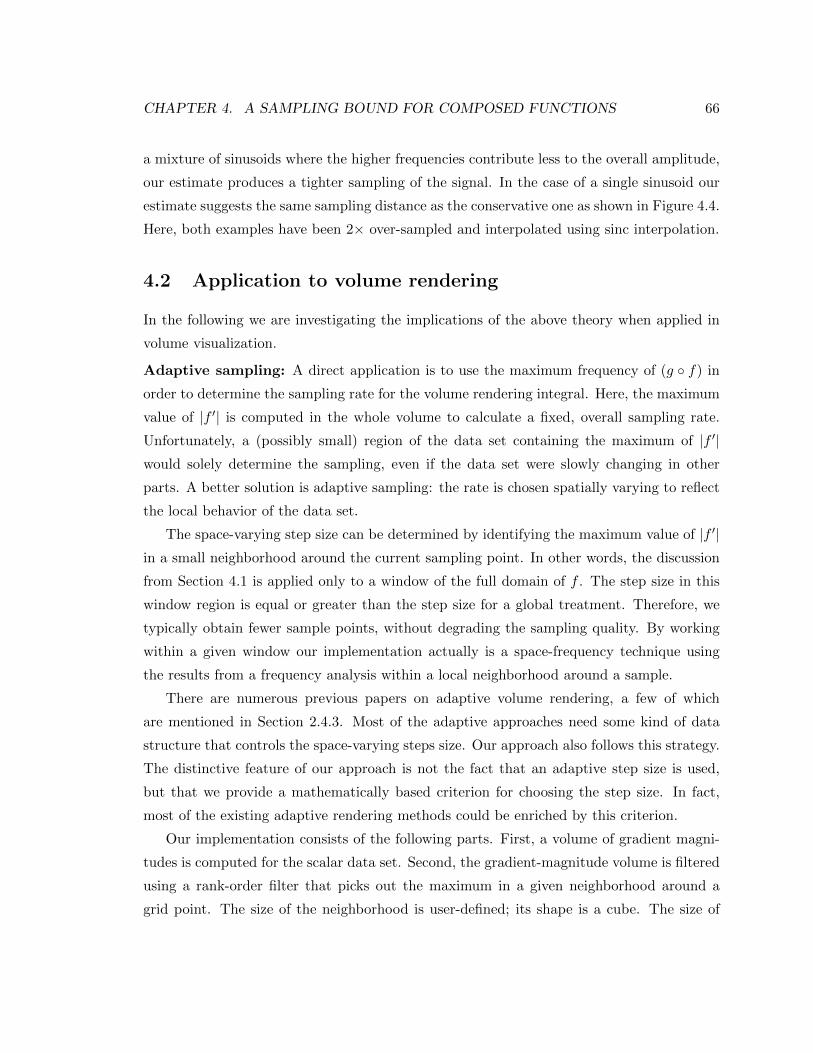
CHAPTER 4. A SAMPLING BOUND FOR COMPOSED FUNCTIONS 66
a mixture of sinusoids where the higher frequencies contribute less to the overall amplitude,
our estimate produces a tighter sampling of the signal. In the case of a single sinusoid our
estimate suggests the same sampling distance as the conservative one as shown in Figure 4.4.
Here, both examples have been 2× over-sampled and interpolated using sinc interpolation.
4.2 Application to volume rendering
In the following we are investigating the implications of the above theory when applied in
volume visualization.
Adaptive sampling: A direct application is to use the maximum frequency of (g f) in
order to determine the sampling rate for the volume rendering integral. Here, the maximum
value of |f ′| is computed in the whole volume to calculate a fixed, overall sampling rate.
Unfortunately, a (possibly small) region of the data set containing the maximum of |f ′|would solely determine the sampling, even if the data set were slowly changing in other
parts. A better solution is adaptive sampling: the rate is chosen spatially varying to reflect
the local behavior of the data set.
The space-varying step size can be determined by identifying the maximum value of |f ′|in a small neighborhood around the current sampling point. In other words, the discussion
from Section 4.1 is applied only to a window of the full domain of f . The step size in this
window region is equal or greater than the step size for a global treatment. Therefore, we
typically obtain fewer sample points, without degrading the sampling quality. By working
within a given window our implementation actually is a space-frequency technique using
the results from a frequency analysis within a local neighborhood around a sample.
There are numerous previous papers on adaptive volume rendering, a few of which
are mentioned in Section 2.4.3. Most of the adaptive approaches need some kind of data
structure that controls the space-varying steps size. Our approach also follows this strategy.
The distinctive feature of our approach is not the fact that an adaptive step size is used,
but that we provide a mathematically based criterion for choosing the step size. In fact,
most of the existing adaptive rendering methods could be enriched by this criterion.
Our implementation consists of the following parts. First, a volume of gradient magni-
tudes is computed for the scalar data set. Second, the gradient-magnitude volume is filtered
using a rank-order filter that picks out the maximum in a given neighborhood around a
grid point. The size of the neighborhood is user-defined; its shape is a cube. The size of
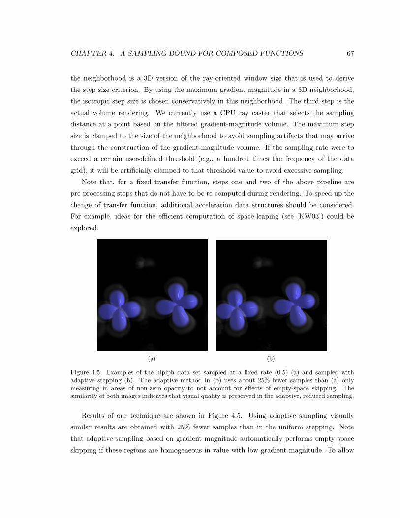
CHAPTER 4. A SAMPLING BOUND FOR COMPOSED FUNCTIONS 67
the neighborhood is a 3D version of the ray-oriented window size that is used to derive
the step size criterion. By using the maximum gradient magnitude in a 3D neighborhood,
the isotropic step size is chosen conservatively in this neighborhood. The third step is the
actual volume rendering. We currently use a CPU ray caster that selects the sampling
distance at a point based on the filtered gradient-magnitude volume. The maximum step
size is clamped to the size of the neighborhood to avoid sampling artifacts that may arrive
through the construction of the gradient-magnitude volume. If the sampling rate were to
exceed a certain user-defined threshold (e.g., a hundred times the frequency of the data
grid), it will be artificially clamped to that threshold value to avoid excessive sampling.
Note that, for a fixed transfer function, steps one and two of the above pipeline are
pre-processing steps that do not have to be re-computed during rendering. To speed up the
change of transfer function, additional acceleration data structures should be considered.
For example, ideas for the efficient computation of space-leaping (see [KW03]) could be
explored.
(a) (b)
Figure 4.5: Examples of the hipiph data set sampled at a fixed rate (0.5) (a) and sampled withadaptive stepping (b). The adaptive method in (b) uses about 25% fewer samples than (a) onlymeasuring in areas of non-zero opacity to not account for effects of empty-space skipping. Thesimilarity of both images indicates that visual quality is preserved in the adaptive, reduced sampling.
Results of our technique are shown in Figure 4.5. Using adaptive sampling visually
similar results are obtained with 25% fewer samples than in the uniform stepping. Note
that adaptive sampling based on gradient magnitude automatically performs empty space
skipping if these regions are homogeneous in value with low gradient magnitude. To allow
CHAPTER 4. A SAMPLING BOUND FOR COMPOSED FUNCTIONS 68
for a fair comparison to uniform sampling stepping we only count samples taken in ranges
of the volume having non-zero opacity. That way the empty space in the images does not
skew the statistics.
For a more quantitative evaluation we have repeated several experiments (using different
sampling distances) for fixed and adaptive sampling and have compared the resulting image
against a ground-truth image, computed at a fixed sampling distance of 0.06125 relative
to a unit grid point spacing of 1. The result of the evaluation is shown in Figure 4.6.
The error plot is based on the signal to noise ratio (SNR), computed as SNR(x,y) =
10 log10
(‖x‖2‖x−y‖2
). We have conducted the image comparison with several different error
metrics, including numeric and perception-based ones. For all metrics the adaptive sampling
clearly outperforms uniform sampling in terms of the number of samples needed to achieve
a given image quality, just like in the SNR-based example given in Figure 4.6.
0 1 2 3 4x 10⁶
0
10
20
30
40
50
60
70
80
90
# samples
Sign
al to
Noise
Rati
o
Quality vs. Performance
adaptiveuniform
Figure 4.6: Quality vs. performance, where quality is measured using signal to noise ratio (SNR)and performance is indicated by the number of samples taken along all rays cast into the volume.Adaptive sampling clearly outperforms the uniform (fixed) sampling. Only samples in areas of non-zero opacity are taken into account, i.e., both sampling schemes equally make use of empty spaceskipping.
For the illustration in Figure 4.7 the adaptive sampling is manually adjusted by multi-
plying a constant (amount of oversampling) onto the suggested sampling distances to match
the number of samples of the uniform sampling Figure 4.7a. This time the numerical error
of both images just matches (both at SNR of about 63). Still, the adaptive sampling shown
in Figure 4.7b has much less prominent artifacts near the surface transition. In case of noisy
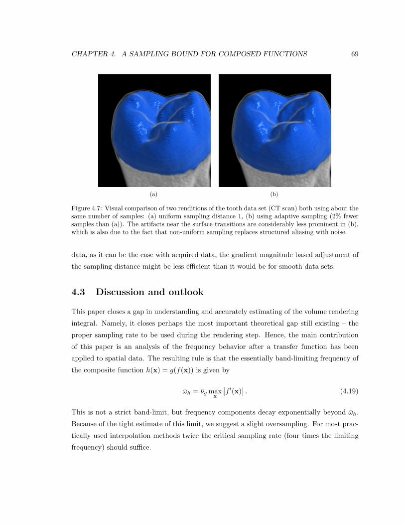
CHAPTER 4. A SAMPLING BOUND FOR COMPOSED FUNCTIONS 69
(a) (b)
Figure 4.7: Visual comparison of two renditions of the tooth data set (CT scan) both using about thesame number of samples: (a) uniform sampling distance 1, (b) using adaptive sampling (2% fewersamples than (a)). The artifacts near the surface transitions are considerably less prominent in (b),which is also due to the fact that non-uniform sampling replaces structured aliasing with noise.
data, as it can be the case with acquired data, the gradient magnitude based adjustment of
the sampling distance might be less efficient than it would be for smooth data sets.
4.3 Discussion and outlook
This paper closes a gap in understanding and accurately estimating of the volume rendering
integral. Namely, it closes perhaps the most important theoretical gap still existing – the
proper sampling rate to be used during the rendering step. Hence, the main contribution
of this paper is an analysis of the frequency behavior after a transfer function has been
applied to spatial data. The resulting rule is that the essentially band-limiting frequency of
the composite function h(x) = g(f(x)) is given by
ωh = νg maxx
∣∣f ′(x)∣∣ . (4.19)
This is not a strict band-limit, but frequency components decay exponentially beyond ωh.
Because of the tight estimate of this limit, we suggest a slight oversampling. For most prac-
tically used interpolation methods twice the critical sampling rate (four times the limiting
frequency) should suffice.

CHAPTER 4. A SAMPLING BOUND FOR COMPOSED FUNCTIONS 70
The treatment in this paper is independent of the application and hence can be applied
in other fields of signal processing and applied mathematics. However, the focus of our
application has been rendering. In addition to the theoretical findings we have applied the
result to a method for adaptive sampling based on the maximum gradient magnitude. We
have been able to apply our theoretical results for an adaptive rendering algorithm that
achieves the same quality in the rendered images by reducing the number of samples needed
significantly.
Conclusion: The effects of composition can be interpreted in different ways. The above
analysis and discussion has considered the mapping of optical properties g(f(x)) on a multi-
field, multi-variate data function f . One can also consider f as a change in parameterization
of g. Both views amount to fundamental data processing operations and an interpretation
of our results beyond the realm of volume graphics seems worthwhile.
Chapter 5
Designing a palette for spectral lighting
In this chapter [BDM09], we employ a more complete spectral representation of
light in a computer graphics setting. This approach allows for more physically
correct renditions of a scene under different lighting conditions. Beyond that,
our prior work [BMDF02] has demonstrated that full spectra allow for additional
visual color effects, that conventional (red,green,blue)-based tri-chromatic rep-
resentations would fail to reproduce.
Giving designers the power to render spectral scenes, also faces them with an
increased challenge to construct them, since classical production pipelines are
typically based on the RGB model. To alleviate this problem this chapter de-
vises a tool to augment a palette of given lights and material reflectances with
additional constructed spectra that yield specified colors. This enables to specif-
ically construct spectral effects such as metamerism or objective color constancy.
We utilize this to emphasize or hide parts of a scene by matching or differen-
tiating colors under different illuminations. These color criteria are expressed
as a quadratic programming problem that can be solved for a globally optimal
solution and can include additional positivity constraints.
The proposed method has the potential to create expressive visualizations. A
key application of our technique is to use specific spectral lighting to scale the
visual complexity of a scene by controlling visibility of texture details in surface
graphics or material details in volume rendering.
71
CHAPTER 5. DESIGNING A PALETTE FOR SPECTRAL LIGHTING 72
Introduction: Light interacting with matter and its processing by the human visual sys-
tem is the basis of imaging. In graphics it is common to simply use RGB values for all
interactions, although it is well known that such a coarse approximation of full spectra can
lead to disastrous errors [JF99]. Hence, for both surface graphics, including transmissions,
as well as volume graphics, we should be using a good approximation of spectra.
Spectra in the context of this chapter will refer to both light as a spectral power distri-
bution (SPD) over different energy levels (wavelengths) of the electromagnetic field, as well
as wavelength dependent reflectance of the material. The latter arises from the fact that
a material reflects or re-emits different wavelengths of incoming light to different degrees.
Both light SPD and reflectance are modeled as scalar functions of wavelength and their basic
interaction can be described as a product of the two, resulting in a reflected spectrum (color
filtering). Additional effects involve shifts in emission of energy towards lower wavelengths
(fluorescence) or at later points in time (phosphorescence). However, in the following we will
consider color filtering alone, since this is the dominant effect if typical current RGB based
photo-realistic scenes are converted and enhanced within a spectral rendering framework.
The field known as physically-based rendering aims at producing photo-realistic im-
agery [PH04b]. Employing an appropriate algorithm that renders a convincingly realistic
impression in practice is only a part of the solution. First, we need a synthetic scene that
contains sufficient detail and has a close correspondence to a physically plausible setting. In
a static setting one can distinguish three aspects: geometric modeling of shapes or density
distribution of volumes, determining material appearance by setting reflection properties,
and configuring the lighting of the scene.
Making a scene: Discrete surface representations can either be acquired from direct sen-
sor measurements [LPC+00] or be extracted indirectly, for instance by depth reconstruc-
tion from multiple images [PKG99, BZS+07] or by matching shape models to individual
pictures [BAZT04, ERT05]. Alternatively, a scene can be modelled manually (e.g., using
Blender or 3D Studio max) or be created procedurally [DHL+98, KM07]. Since the creation
of synthetic geometry has already received significant attention in research, we will focus,
in the following, on the creation of synthetic materials.
Consequences of changing the light model: When switching the light model from RGB
(red, green, blue) components to a spectral representation, the geometric modeling remains
unaffected. Also, directional dependence of material shading properties as it is expressed by
CHAPTER 5. DESIGNING A PALETTE FOR SPECTRAL LIGHTING 73
a bi-directional reflection distribution function (BRDF) can still be used. However, modeling
the wavelength dependence of the BRDF as well as the light requires a new tool replacing
the classical color picker.
While in the classical approach the reflectance or the light spectra are chosen separately,
what we often need to model is the result of their interaction. In other words, we would like
to input the resulting light-reflectance interaction as a constraint into our modeling system
and have the system choose proper materials and lights.
The design tool devised in this chapter is not limited to picking specific colors for cer-
tain light-material combinations. As well as that, it is aimed at taking advantage of certain
effects that are inherent to the use of spectra. They are based on the notion of metamers
— materials that look the same under one light, but may have clearly distinguishable color
under another. In typical color matching problems metamerism is increased to make mate-
rials match under different lights. Our goal is to ensure metamerism only for one light, but
to exploit the visual effect when the reflectances do not match if illuminated with a different
light source. This can be employed to control visibility of additional detail in a scene as will
be shown for a surface graphics example in § 5.4.3.
Another effect is that of a metameric black [WS82] a surface spectral reflectance function
that produces a zero RGB triple under a particular light. Under another light the surface
appears colored, not black. Highly (but not completely) transparent materials tend to
virtually disappear from a scene when they turn black. Another light that is reflected
brightly may bring their appearance back to the user’s attention. The question of how to
incorporate such behavior into the design of spectra is the subject of § 5.2.
The obverse of the situation is one in which a user controls the appearance of a scene
by changing the lighting. In a design involving metameric blacks as the difference between
reflectances those materials retain their color as the light changes — we refer to this as
objective color constancy. Then clearly, if one material is designed to change appearance, as
the lights change, while other materials stay the same, we have a means to guide the user’s
attention, which can be used for the exploration of data sets.
Sampling the visible spectrum from 400 nm to 700 nm in 10 nm steps results in a
31-component spectral representation. Instead of our usual 3-vector component-wise multi-
plication, we have an order of magnitude more computational work. In a raytracing scenario
where we may have billions of light-material interactions this will be very computationally
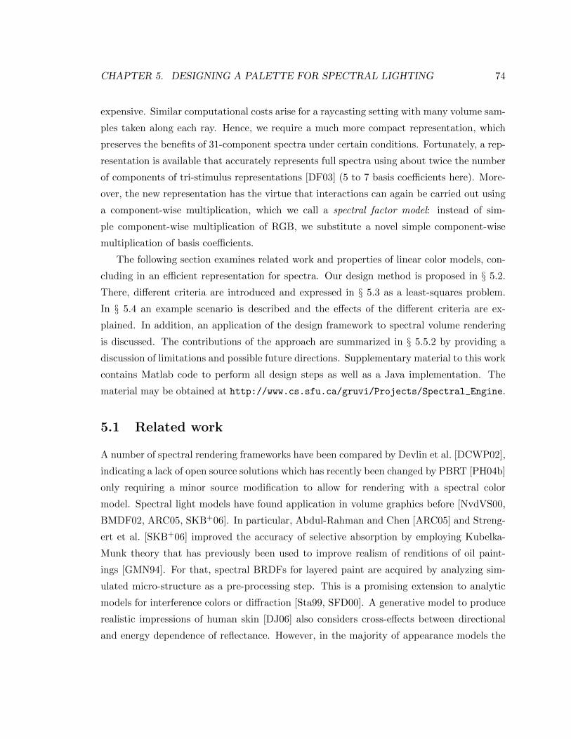
CHAPTER 5. DESIGNING A PALETTE FOR SPECTRAL LIGHTING 74
expensive. Similar computational costs arise for a raycasting setting with many volume sam-
ples taken along each ray. Hence, we require a much more compact representation, which
preserves the benefits of 31-component spectra under certain conditions. Fortunately, a rep-
resentation is available that accurately represents full spectra using about twice the number
of components of tri-stimulus representations [DF03] (5 to 7 basis coefficients here). More-
over, the new representation has the virtue that interactions can again be carried out using
a component-wise multiplication, which we call a spectral factor model: instead of sim-
ple component-wise multiplication of RGB, we substitute a novel simple component-wise
multiplication of basis coefficients.
The following section examines related work and properties of linear color models, con-
cluding in an efficient representation for spectra. Our design method is proposed in § 5.2.
There, different criteria are introduced and expressed in § 5.3 as a least-squares problem.
In § 5.4 an example scenario is described and the effects of the different criteria are ex-
plained. In addition, an application of the design framework to spectral volume rendering
is discussed. The contributions of the approach are summarized in § 5.5.2 by providing a
discussion of limitations and possible future directions. Supplementary material to this work
contains Matlab code to perform all design steps as well as a Java implementation. The
material may be obtained at http://www.cs.sfu.ca/gruvi/Projects/Spectral_Engine.
5.1 Related work
A number of spectral rendering frameworks have been compared by Devlin et al. [DCWP02],
indicating a lack of open source solutions which has recently been changed by PBRT [PH04b]
only requiring a minor source modification to allow for rendering with a spectral color
model. Spectral light models have found application in volume graphics before [NvdVS00,
BMDF02, ARC05, SKB+06]. In particular, Abdul-Rahman and Chen [ARC05] and Streng-
ert et al. [SKB+06] improved the accuracy of selective absorption by employing Kubelka-
Munk theory that has previously been used to improve realism of renditions of oil paint-
ings [GMN94]. For that, spectral BRDFs for layered paint are acquired by analyzing sim-
ulated micro-structure as a pre-processing step. This is a promising extension to analytic
models for interference colors or diffraction [Sta99, SFD00]. A generative model to produce
realistic impressions of human skin [DJ06] also considers cross-effects between directional
and energy dependence of reflectance. However, in the majority of appearance models the
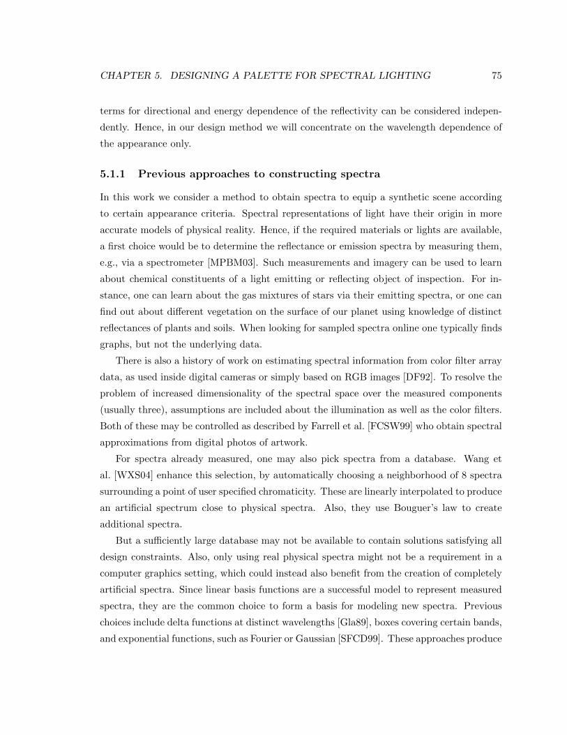
CHAPTER 5. DESIGNING A PALETTE FOR SPECTRAL LIGHTING 75
terms for directional and energy dependence of the reflectivity can be considered indepen-
dently. Hence, in our design method we will concentrate on the wavelength dependence of
the appearance only.
5.1.1 Previous approaches to constructing spectra
In this work we consider a method to obtain spectra to equip a synthetic scene according
to certain appearance criteria. Spectral representations of light have their origin in more
accurate models of physical reality. Hence, if the required materials or lights are available,
a first choice would be to determine the reflectance or emission spectra by measuring them,
e.g., via a spectrometer [MPBM03]. Such measurements and imagery can be used to learn
about chemical constituents of a light emitting or reflecting object of inspection. For in-
stance, one can learn about the gas mixtures of stars via their emitting spectra, or one can
find out about different vegetation on the surface of our planet using knowledge of distinct
reflectances of plants and soils. When looking for sampled spectra online one typically finds
graphs, but not the underlying data.
There is also a history of work on estimating spectral information from color filter array
data, as used inside digital cameras or simply based on RGB images [DF92]. To resolve the
problem of increased dimensionality of the spectral space over the measured components
(usually three), assumptions are included about the illumination as well as the color filters.
Both of these may be controlled as described by Farrell et al. [FCSW99] who obtain spectral
approximations from digital photos of artwork.
For spectra already measured, one may also pick spectra from a database. Wang et
al. [WXS04] enhance this selection, by automatically choosing a neighborhood of 8 spectra
surrounding a point of user specified chromaticity. These are linearly interpolated to produce
an artificial spectrum close to physical spectra. Also, they use Bouguer’s law to create
additional spectra.
But a sufficiently large database may not be available to contain solutions satisfying all
design constraints. Also, only using real physical spectra might not be a requirement in a
computer graphics setting, which could instead also benefit from the creation of completely
artificial spectra. Since linear basis functions are a successful model to represent measured
spectra, they are the common choice to form a basis for modeling new spectra. Previous
choices include delta functions at distinct wavelengths [Gla89], boxes covering certain bands,
and exponential functions, such as Fourier or Gaussian [SFCD99]. These approaches produce
CHAPTER 5. DESIGNING A PALETTE FOR SPECTRAL LIGHTING 76
mixtures of three functions for red, green and blue (RGB). To obtain flatter spectra [Smi99]
also includes complementary colors (CMY).
All of the above methods to create artificial spectra have one common problem: they
consider the design of a reflectance for a given color without considering the illumination
spectrum. Such a design essentially only applies in controlling the appearance of self emitting
objects. But for typical materials it is only the reflected spectra that we can see. These are
related to the light spectrum, via a product with the wavelength dependent reflectance, but
they are not the same. Thus, the color of a surface should indeed be chosen with respect
to the reflected spectrum, but what really needs to be assigned in the scene description is a
reflectance and a light.
This observation is the main motivation for our design method. The second main dif-
ference over previous methods is that we consider a design of an entire palette of several
reflectances and lights instead of just single combination colors. This allows us to take ef-
fects of combined material appearance or lighting transitions into account. In the following,
we will provide some background on linear color models, leading to a choice of basis for
efficient component-wise illumination computations, called the spectral factor model. The
design method and its description in § 5.2, however, are independent of a particular choice
of linear model.
5.1.2 Linear light models
Linear representations for spectra of lights and reflectances are attractive for rendering com-
plex scenes for several reasons. Firstly, all illumination calculations can be performed in a
linear subspace of reduced dimensionality; and the basis can be specialized for a set of rep-
resentative spectra, thus improving accuracy. In general, each illumination computation in
the linear subspace implies a matrix multiplication. The following discussion will construct
this illumination matrix R.
The basic idea of using a linear model is to describe a spectrum C(λ) (e.g., a color
signal [WS82] formed from the product of light and surface spectral reflectance functions)
by a linear combination of a set of basis functions Bi weighted by coefficients ci:
C(λ) =
m∑i=1
ciBi(λ). (5.1)
CHAPTER 5. DESIGNING A PALETTE FOR SPECTRAL LIGHTING 77
The choice of basis functions can be guided by different criteria. Marimont and Wan-
dell [MW92] discuss different approaches to finding a basis that minimizes perceivable errors
in the sensor responses. Peercy [Pee93] devised a framework for using linear color models in
illumination calculations. The quality of a particular basis can be summarized as the trade-
off between accuracy and computational complexity. There are two different approaches
to this issue. We can form specialized bases tailored to the particular set of spectra in a
scene. Then these spectra have only minimal error when projected to the subspace spanned
by the linear model. Spectra differing from the prototype spectra may have larger error
from projection. Alternatively, general bases are suitable for a wider set of spectra. For
instance, using exponential functions, such as a Fourier basis, only assumes some degree of
smoothness of the modeled spectra. Certainly, all spectra that are smooth enough will be
well represented; however, a Fourier representation may have negative coefficients for valid
physical (i.e., nonnegative) spectra, making the model problematic to use in a hardware
implementation.
In order to computationally model interactions between spectral power distributions
(SPDs) we represent the power distribution C(λ) as a discrete vector. A full spectrum then
consists of equidistant point samples taken over the visible range from 400 nm to 700 nm
at 10 nm intervals forming a vector ~C ∈ R31. The basis in Eq. 5.1 then becomes a 31 ×mmatrix B comprised of the set of m basis vectors ~Bi and the coefficients ci become a vector
~c approximating Eq. 5.1 as
~C =m∑i=1
ci ~Bi = B~c. (5.2)
Modeling illumination we will restrict ourselves to non-fluorescent interactions — no
energy is shifted along different wavelengths of the spectrum. Hence, the observed reflected
color spectrum equals a component-wise product of the two SPDs. We will use diag(~S) as
a diagonal matrix composed of the elements of ~S to define a component-wise multiplication
operator ∗ between ~E and ~S:
~C = diag( ~E) ~S = diag(~S) ~E = ~E ∗ ~S = ~S ∗ ~E. (5.3)
The coefficients ~c for a spectrum ~C can be obtained via the pseudo-inverse B+ of B defined
in Equation B.13:
~c = B+ ~C. (5.4)
CHAPTER 5. DESIGNING A PALETTE FOR SPECTRAL LIGHTING 78
The spectra forming ~C can also be expressed in the linear subspace as ~S =m∑k=1
sk ~Bk and
similarly ~E. We combine the previous equations:
ci = ~B+
i (
m∑j=1
ej ~Bj ∗m∑k=1
sk ~Bk). (5.5)
The two operands inside the parentheses are ~E and ~S from Eq. 5.3. The result of the spectral
multiplication (in the full space R31) is then projected back onto the basis functions, as in
Eq. 5.4. The vector ~B+
i denotes the ith row of the inverted basis B+. By reordering, we
obtain
ci = ~B+
i
m∑j=1
m∑k=1
( ~Bj ∗ ~Bk) ejsk. (5.6)
This equation can be rewritten as a matrix multiplication, but one of the two coefficient
vectors has to be integrated into it. To do so, we define a new matrix R written in terms
of either ~s or ~e:
~c = R(~s)~e = R(~e)~s,
with Rij(~v) = ~B+
i
m∑k=1
( ~Bj ∗ ~Bk) vk (5.7)
The m × m matrix R carries out any reflectance computation inside the linear subspace.
Equation 5.7 also shows that an arbitrary choice of some basis does not necessarily lead to
a diagonalization of R. However, it is at least possible to use specialized hardware to apply
this matrix at every reflection event [PZB95]. Current commodity graphics hardware do
also allow for an implementation using the GPU.
In the following, we discuss how to modify the basis functions such that componentwise
multiplications alone, with diagonalization of R, will suffice for such computations.
5.1.3 Accuracy
One problem with using linear models is that only the spectra from which the basis functions
are derived are likely to be represented with good accuracy. For this we make use of principal
component analysis (PCA) for a set of given spectra, and the first m significant vectors are
taken to span an orthonormal linear subspace for the spectra. Other spectra, which have
not been considered during the construction of this basis may be very different from their
CHAPTER 5. DESIGNING A PALETTE FOR SPECTRAL LIGHTING 79
projections into that space.
Particularly in the case of fluorescent (spiky) lights or sharp cutoff bands, we should
make use of a dedicated, or ‘specialized’, basis. Each illumination step as described in
Eq. 5.7 makes use of a result projected back into the linear subspace and hence at every
interaction the linear representation may move farther from an accurate representation of
the product spectrum. This problem is especially relevant if we use multiple scattering or
spectral volume absorption. The highest accuracy is achieved when only very few illumina-
tion calculations are performed. In case of a local illumination model in combination with
‘flat’ absorption (alpha blending), only one scattering event is considered with no further
transmission events. Another technique especially appropriate for linear color models is
sub-surface scattering [HK93]. This method uses only very few reflections beneath a sur-
face. Yet the spectral absorption (participating medium) is important for realistic results, so
using spectra can greatly improve correctness; since there are only relatively few absorption
events the accuracy is still acceptable.
5.2 Designing spectra
The technique described in this section seeks to extend a scene containing real world re-
flectance and light spectra by creating additional artificial materials and lights that fulfill
certain criteria:
1. a constructed light/reflectance should produce user-chosen colors in combination with
given reflectances/lights;
2. spectra may also be represented in a lower dimensional linear subspace model for
which the approximation error should be minimal;
3. to regularize the solution we minimize the second order difference of the discrete
spectrum; this provides smoothness of the solution and improves convergence;
4. physically plausible spectra should be positive, which enters the optimization as a
lower bound constraint.
The first three of these points are expressed as linear least squares problems. This allows
us to weight and combine different criteria and to employ standard solution methods.
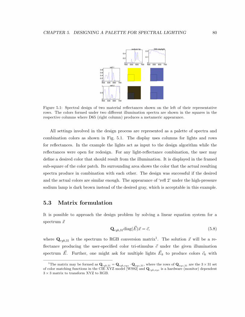
CHAPTER 5. DESIGNING A PALETTE FOR SPECTRAL LIGHTING 80
400 500 600 7000
0.2
0.40.6
0.8
400 500 600 7000
0.5
1
400 500 600 7000
0.2
0.4
400 500 600 7000
0.1
0.2
refl 1
refl 2
sodium hp D65 daylight
Figure 5.1: Spectral design of two material reflectances shown on the left of their representativerows. The colors formed under two different illumination spectra are shown in the squares in therespective columns where D65 (right column) produces a metameric appearance.
All settings involved in the design process are represented as a palette of spectra and
combination colors as shown in Fig. 5.1. The display uses columns for lights and rows
for reflectances. In the example the lights act as input to the design algorithm while the
reflectances were open for redesign. For any light-reflectance combination, the user may
define a desired color that should result from the illumination. It is displayed in the framed
sub-square of the color patch. Its surrounding area shows the color that the actual resulting
spectra produce in combination with each other. The design was successful if the desired
and the actual colors are similar enough. The appearance of ‘refl 2’ under the high-pressure
sodium lamp is dark brown instead of the desired gray, which is acceptable in this example.
5.3 Matrix formulation
It is possible to approach the design problem by solving a linear equation system for a
spectrum ~x
Qrgb,31diag( ~E)~x = ~c, (5.8)
where Qrgb,31 is the spectrum to RGB conversion matrix1. The solution ~x will be a re-
flectance producing the user-specified color tri-stimulus ~c under the given illumination
spectrum ~E. Further, one might ask for multiple lights ~Ek to produce colors ~ck with
1The matrix may be formed as Qrgb,31 = Qrgb,xyz ·Qxyz,31, where the rows of Qxyz,31 are the 3× 31 setof color matching functions in the CIE XYZ model [WS82] and Qrgb,xyz is a hardware (monitor) dependent3× 3 matrix to transform XYZ to RGB.
CHAPTER 5. DESIGNING A PALETTE FOR SPECTRAL LIGHTING 81
reflectance ~x. One can solve for this by vertically concatenating the illumination matrices
Qrgb,31diag( ~Ek) = Q( ~Ek)rgb,31 into a matrix M and their respective color forcing vectors ~ck into
a vector ~y. As there might not be a spectrum that fulfills all conditions exactly we switch
from solving an equation system to a quadratic minimization problem:
min~x||M~x− ~y|| = min~x
[~xTMTM~x− 2~yTM~x
], (5.9)
An unconstrained solution would be available via the pseudo-inverse M+ = (MTM)−1M
as ~x = M+~y. Alternatively, we use quadratic programming (QP), because it allows the
inclusion of lower and upper bound constraints for the components of ~x. Note that the
entire design could be carried out, such that ~x gives a light ~E instead of a reflectance ~S, by
replacing ~E with ~S in Eq. 5.8. The solution ~x would then contain a light ~E producing color
~c when illuminating the given reflectance ~S. This outlines the main idea behind the design
method. We will refine it in the following by adding more optional criteria, such as linear
subspace model error minimization and smoothness via minimal second order differences.
Finally, all criteria are weighted and combined by concatenating them to form M and ~y in
a single QP problem.
As shown in § 5.1.2, color computation can also be performed in the linear subspace. The
3×m matrix that takes an m-vector representation in basis B of Eq. 5.2 directly to RGB
is Qrgb,m = Qrgb,31 B. The least squares problem that minimizes the error when computing
illumination in the subspace is expressed as:
min~s‖Qrgb,mR(~e)~s− ~c‖, corresponds to
min~S‖Q( ~E)
rgb,m,31~S − ~c‖, with
Q( ~E)rgb,m,31 = Qrgb,m R(Qm,31
~E) Qm,31, (5.10)
where R(~e) is the matrix from Eq. 5.7 that performs the illumination calculation of light ~E
and surface ~S using their Rm subspace representations ~e = Qm,31~E or ~s in analog form.
From the previous discussion we can express color objectives for illumination in the
point sampled 31-dimensional spectral model and in the m-dimensional subspace model.
The following criterion seeks to minimize the difference between the resulting colors from
CHAPTER 5. DESIGNING A PALETTE FOR SPECTRAL LIGHTING 82
these two illumination methods to be close to a zero 3-vector ~03:
min~S‖F( ~E) ~S −~03‖, (5.11)
F( ~E) = Q( ~E)rgb,31 −Q
( ~E)rgb,m,31. (5.12)
The third criterion is smoothness. While the previous two criteria are aimed at accurate
color reproduction, this one is introduced to allow control over the general shape of the
spectrum and to provide regularization reducing the search space of the optimization. An
optimal solution for given design colors with minimum error can lead to spiky spectra with
large extrema. A commonly used indicator for roughness of a curve is the integral over
the squared second derivative or second order differences in our discretized model. Other
indicators are possible, but this one can easily be expressed in the following form:
min~S‖D ~S −~031‖, with
D = Toeplitz([ −1 2 −1 0 · · · 0 ]) , ~031 = zero 31-vector. (5.13)
D is a tri-diagonal matrix having 3-vector [−1, 2, −1] on the three middle diagonals and zero
everywhere else, which is also called a Toeplitz matrix. The whole matrix D is normalized
by 1/(√
31 ‖ − 1 2 − 1‖): the√
31 takes care of the number of rows of the matrix so as not
to make smoothness more important than the design color matrices. Those we normalize
by 1/√
3 in order to have comparable importance. This is relevant when the residues of all
above criteria are combined in a sum of squares, as we will discuss next.
5.3.1 Combined optimization function
Each of the design criteria is expressed as one of the matrices Q( ~X)rgb,31,Q
( ~X)rgb,m,31,F,D with
accompanying objective vectors (target colors or zero vectors). The design matrix M is
formed by vertically concatenating these criteria matrices. Similarly, the associated forcing
vectors are stacked to form ~y. The different criteria are weighted by ωij|F |D for design
colors ~cij , error matrix F, and smoothness D respectively. These weights provide control
over the convergence of the minimization and may all be set to 1. We compute a minimum
error solution for an overdetermined system Mi ~x = ~yi for a surface ~Si corresponding to the
CHAPTER 5. DESIGNING A PALETTE FOR SPECTRAL LIGHTING 83
set of stacked equations: ωi1Q( ~E1)rgb,31
ωFωi1F( ~E1)
ωDD
· ~x = ~y =
ωi1~ci1
~03
~031
, (5.14)
We solve this system for a minimum error solution using the form of Eq. 5.9. The solution
~x will contain the desired reflectance ~Si producing color ~ci1 with light ~E1. If there are
several colors that should be produced in combination with different lights ~Ej , the upper
two blocks are vertically repeated for each ~Ej , since the smoothness criterion D only needs
to be included once. In the following we will consider the simultaneous creation of several
spectra.
5.3.2 Free metamers
In the above formulation the design of one spectrum ~Si is independent of the other spectra
that are to be designed. However, it is possible to solve for all needed spectra simultane-
ously, by combining their individual design matrices Mi in a direct sum. This means to
concatenate the matrices diagonally and to fill the remaining elements with zeros ∅ in the
form M = [M1 ∅; ∅M2], where the semicolon denotes vertical concatenation. The respec-
tive forcing vectors ~yi are stacked as well and the solution vector ~x will contain several
spectra concatenated.
We will use this to include ’free’ colors into the design: we create two spectra ~Si, ~Sj
and instead of defining their desired color as part of ~y, we will leave the actual color open
and retrieve it as part of the solution in ~x. This is useful if we want those two reflectances
to look the same under a light ~Ea, but do not care what specific color they will actually
form as long as they are metameric. This can then be combined with further design colors
for a different light ~Eb. More formally, we solve for a weighted solution ~cia, ~Si, ~Sj of the
system
Q( ~Ea)rgb,31
~Si = Q( ~Ea)rgb,31
~Sj ,
Q( ~Eb)rgb,31
~Si = ~cib
(5.15)
using an illumination matrix as defined after Eq. 5.8 and with color ~cib given for a surface
~Si under light ~Eb: i.e., we ask this surface ~Si under another light ~Ea to have the same color
CHAPTER 5. DESIGNING A PALETTE FOR SPECTRAL LIGHTING 84
as surface ~Sj under that light. As a stacked matrix Eq. 5.15 becomes
−ωia 0 0 ~031
0 −ωia 0 ωiaQ( ~Ea)rgb,31
~031
0 0 −ωia ~031
−ωja 0 0 ~031
0 −ωja 0 ~031 ωjaQ( ~Ea)rgb,31
0 0 −ωja ~031
0 0 0 ~031
0 0 0 ωibQ( ~Eb)rgb,31
~031
0 0 0 ~031
· ~x = ~y =
~03
~03
ωib~cib
. (5.16)
The involved weights ω can be changed from the default value 1 to steer the importance
of this color criterion over others. The resulting ~x contains the ‘free’ color ~cia = ~cja in the
first three components, and after that two 31-component vectors for reflectances ~Si and ~Sj .
This setup becomes interesting when used with upper and lower bounds on ~x, because then
the ‘free’ color can be forced into a given interval without being specified precisely. The
blue metameric color under light D65 in Fig. 5.1 was obtained using this method.
5.4 Evaluation and visual results
In the following, we will demonstrate the use of our spectral design method in several
contexts. We will start with a palette design, followed by an error evaluation for different
design conditions. Beyond considering palettes by themselves we will also show their use
in practical spectral rendering examples in 3D surface graphics and volume rendering. The
set of Matlab scripts for the design method and example setups of this paper along with a
Java version of the spectrum generator are available as supplementary material at the URL
given at the end of the introduction.
CHAPTER 5. DESIGNING A PALETTE FOR SPECTRAL LIGHTING 85
5.4.1 Example palette design
An example palette design is shown in Fig. 5.2. The target colours (shown in the framed
sub-squares) under the light in the third column were taken from a palette of the Color
Brewer tool [HB03]. A light fulfilling these colours is generated with our method and is
denoted SplitLight 2. The center column colours are chosen to visually merge each of the
two red tones in column 3 and separate the two blue tones, replacing them by their average.
These colours result when switching to designed illuminant SplitLight 1. In contrast, the
first column, illuminated by measured standard daylight D65, is set to a single metameric
average colour for all five reflectances. The spectra of the two artificial ‘split light’ sources are
initially chosen as shifted positive sine waves of different period lengths (60nm and 85nm).
For the setup the smoothness weight ωD was set to 1 and subspace error minimization was
omitted. All light sources are initially normalized to a luminance Y = 6 and the reflectances
are allowed to have magnitudes in [0, 1]. This scaling factor was determined experimentally
through a preliminary unbounded design.
In a first design phase we create reflectances fulfilling the given colours. Here, we choose
importance weights ωi,1 = 4 for the first column, leaving the remaining weights at 1. This
gives correct metamers under daylight D65 and gets the remaining palette colours approxi-
mately right. In a second phase we use the newly created reflectances to re-create the two
‘split lights’ to produce the given colours more exactly. The resulting spectra are shown in
the graphs in Fig. 5.2.
5.4.2 Design error with respect to number of constraints
Expressing the design criteria as soft constraints allows us to always obtain a solution, but
possibly with errors depending on how well the criteria agree with each other. In order to
obtain a better understanding of these errors we performed a number of automated tests
on palettes of varying sizes. For each of the tests (with errors displayed in Fig. 5.3), we are
requesting fixed random combination colours between each reflectance and light (uniformly
distributed in RGB space). Lights and reflectance are formed by first creating reflectances
for fixed random lights and then re-computing lights for the new reflectances. The bottom
left and right axes of each graph in Fig. 5.3 indicate the numbers of reflectances and lights,
respectively. The vertical axis denotes the average L∗a∗b∗ distance between designed and
actual light-reflectance combination colours over the entire palette of a given size. While
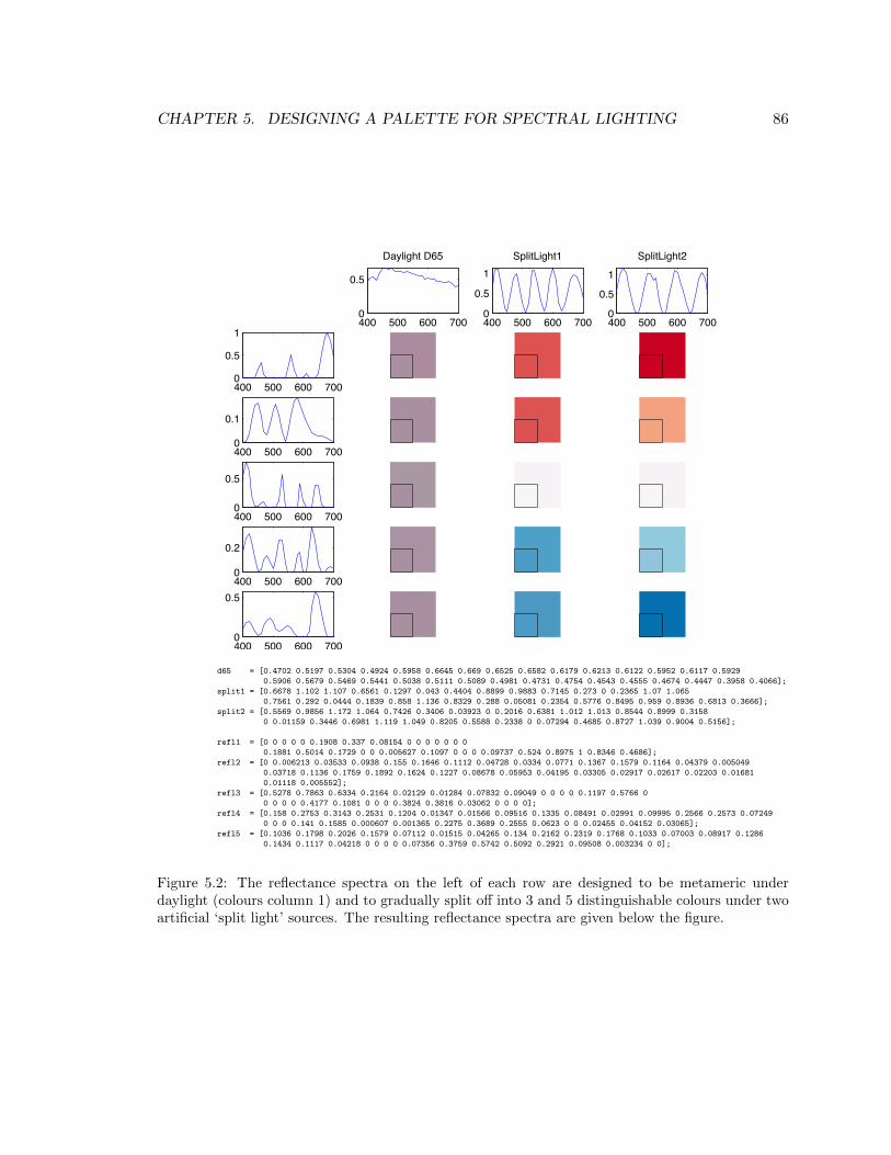
CHAPTER 5. DESIGNING A PALETTE FOR SPECTRAL LIGHTING 86
400 500 600 7000
0.5
1
400 500 600 7000
0.1
400 500 600 7000
0.5
400 500 600 7000
0.2
400 500 600 7000
0.5
400 500 600 7000
0.5
Daylight D65
400 500 600 7000
0.5
1
SplitLight1
400 500 600 7000
0.5
1
SplitLight2
d65 = [0.4702 0.5197 0.5304 0.4924 0.5958 0.6645 0.669 0.6525 0.6582 0.6179 0.6213 0.6122 0.5952 0.6117 0.5929
0.5906 0.5679 0.5469 0.5441 0.5038 0.5111 0.5089 0.4981 0.4731 0.4754 0.4543 0.4555 0.4674 0.4447 0.3958 0.4066];
split1 = [0.6678 1.102 1.107 0.6561 0.1297 0.043 0.4404 0.8899 0.9883 0.7145 0.273 0 0.2365 1.07 1.065
0.7561 0.292 0.0444 0.1839 0.858 1.136 0.8329 0.288 0.05081 0.2354 0.5776 0.8495 0.959 0.8936 0.6813 0.3666];
split2 = [0.5569 0.9856 1.172 1.064 0.7426 0.3406 0.03923 0 0.2016 0.6381 1.012 1.013 0.8544 0.8999 0.3158
0 0.01159 0.3446 0.6981 1.119 1.049 0.8205 0.5588 0.2338 0 0.07294 0.4685 0.8727 1.039 0.9004 0.5156];
refl1 = [0 0 0 0 0 0.1908 0.337 0.08154 0 0 0 0 0 0 0
0.1881 0.5014 0.1729 0 0 0.005627 0.1097 0 0 0 0.09737 0.524 0.8975 1 0.8346 0.4686];
refl2 = [0 0.006213 0.03533 0.0938 0.155 0.1646 0.1112 0.04728 0.0334 0.0771 0.1367 0.1579 0.1164 0.04379 0.005049
0.03718 0.1136 0.1759 0.1892 0.1624 0.1227 0.08678 0.05953 0.04195 0.03305 0.02917 0.02617 0.02203 0.01681
0.01118 0.005552];
refl3 = [0.5278 0.7863 0.6334 0.2164 0.02129 0.01284 0.07832 0.09049 0 0 0 0 0.1197 0.5766 0
0 0 0 0 0.4177 0.1081 0 0 0 0.3824 0.3816 0.03062 0 0 0 0];
refl4 = [0.158 0.2753 0.3143 0.2531 0.1204 0.01347 0.01566 0.09516 0.1335 0.08491 0.02991 0.09995 0.2566 0.2573 0.07249
0 0 0 0.141 0.1585 0.000607 0.001365 0.2275 0.3689 0.2555 0.0623 0 0 0.02455 0.04152 0.03065];
refl5 = [0.1036 0.1798 0.2026 0.1579 0.07112 0.01515 0.04265 0.134 0.2162 0.2319 0.1768 0.1033 0.07003 0.08917 0.1286
0.1434 0.1117 0.04218 0 0 0 0 0.07356 0.3759 0.5742 0.5092 0.2921 0.09508 0.003234 0 0];
Figure 5.2: The reflectance spectra on the left of each row are designed to be metameric underdaylight (colours column 1) and to gradually split off into 3 and 5 distinguishable colours under twoartificial ‘split light’ sources. The resulting reflectance spectra are given below the figure.
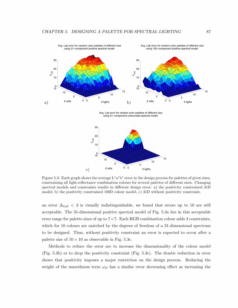
CHAPTER 5. DESIGNING A PALETTE FOR SPECTRAL LIGHTING 87
a)0
510
15
0
5
10
150
10
20
30
# ligths
Avg. Lab error for random color palettes of different sizeusing 31−component positive spectral model
# refls
ΔLa
b
b)0
510
15
0
5
10
150
10
20
30
# ligths
Avg. Lab error for random color palettes of different sizeusing 100−component positive spectral model
# refls
ΔLa
b
c)0
510
15
0
5
10
150
10
20
30
# ligths
Avg. Lab error for random color palettes of different sizeusing 31−component unbounded spectral model
# refls
ΔLa
b
Figure 5.3: Each graph shows the average L∗a∗b∗ error in the design process for palettes of given sizes,constraining all light-reflectance combination colours for several palettes of different sizes. Changingspectral models and constraints results in different design error: a) the positivity constrained 31Dmodel, b) the positivity constrained 100D colour model, c) 31D without positivity constraint.
an error ∆Lab < 3 is visually indistinguishable, we found that errors up to 10 are still
acceptable. The 31-dimensional positive spectral model of Fig. 5.3a lies in this acceptable
error range for palette sizes of up to 7×7. Each RGB combination colour adds 3 constraints,
which for 10 colours are matched by the degrees of freedom of a 31-dimensional spectrum
to be designed. Thus, without positivity constraint an error is expected to occur after a
palette size of 10× 10 as observable in Fig. 5.3c.
Methods to reduce the error are to increase the dimensionality of the colour model
(Fig. 5.3b) or to drop the positivity constraint (Fig. 5.3c). The drastic reduction in error
shows that positivity imposes a major restriction on the design process. Reducing the
weight of the smoothness term ωD has a similar error decreasing effect as increasing the
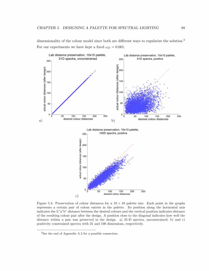
CHAPTER 5. DESIGNING A PALETTE FOR SPECTRAL LIGHTING 88
dimensionality of the colour model since both are different ways to regularize the solution.2
For our experiments we have kept a fixed ωD = 0.001.
a)
0 50 100 150 200 2500
50
100
150
200
250
desired colour distances
actu
al c
olou
r dis
tanc
es (a
fter d
esig
n)
Lab distance preservation, 10x10 palette, 31D spectra, unconstrained
b)0 50 100 150 200 250
0
50
100
150
200
250
desired colour distancesac
tual
col
our d
ista
nces
(afte
r des
ign)
Lab distance preservation, 10x10 palette, 31D spectra, positive
c)
0 50 100 150 200 2500
50
100
150
200
250
desired colour distances
actu
al c
olou
r dis
tanc
es (a
fter d
esig
n)
Lab distance preservation, 10x10 palette, 100D spectra, positive
Figure 5.4: Preservation of colour distances for a 10 × 10 palette size. Each point in the graphsrepresents a certain pair of colour entries in the palette. Its position along the horizontal axisindicates the L∗a∗b∗ distance between the desired colours and the vertical position indicates distanceof the resulting colour pair after the design. A position close to the diagonal indicates how well thedistance within a pair was preserved in the design. a) 31-D spectra, unconstrained; b) and c)positivity constrained spectra with 31 and 100 dimensions, respectively.
2See the end of Appendix A.2 for a possible connection.

CHAPTER 5. DESIGNING A PALETTE FOR SPECTRAL LIGHTING 89
Preserving distance between colours: When setting up several colours a designer some-
times need not closely specify just what colour is actually produced, but rather that the
colours of two objects should be very similar or notably different. This idea is the motivation
for our second type of evaluation. Here, we do not look at the preservation of the actual
colour in the design, but rather the distances between them. In an N ×M palette setup,
we consider each of the 12(N ×M)2 colour pairs, excluding duplicate pairings.
In particular, we want to see how well the (perceptual) distance between the desired
colours matches the (perceptual) distance between the actual colours produced by the de-
signed spectra. Similar to the previous analysis, the evaluation in Fig. 5.4 shows that posi-
tivity is a rather strong constraint, but that increasing the dimensionality of the underlying
spectral model can be used to compensate for it.
5.4.3 Spectral surface graphics
a) b)
Figure 5.5: Car model rendered with PBRT. (a) The spectral materials used in the texture aremetameric under daylight D65, resulting in a monochrome appearance. (b) Changing the illumina-tion spectrum to that of a high pressure sodium lamp, as used in street lighting, breaks apart themetamerism and reveals additional visual information.
To implement spectral raytracing we have used the physically based rendering toolkit
(PBRT) [PH04b]. Its modular design allows us to easily extend the colour model to a 31
component linear model with the appropriate colour space transformation matrices. Also,
we have added support to load spectral textures, and a Python script to replace RGB values
by linear combinations of red, green, and blue spectra to facilitate rendering of conventional
RGB scenes with the modified spectral renderer. Fig. 5.5 shows two impressions of the same
scene under different illumination. Lighting is provided by an area light source emitting one
of the two illumination spectra of Fig. 5.1. The spectral texture for the flame job on the
side of the car uses the reflectances from the same palette. Thus, the daylight metamerism
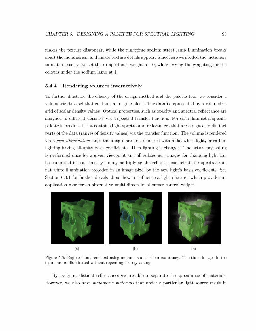
CHAPTER 5. DESIGNING A PALETTE FOR SPECTRAL LIGHTING 90
makes the texture disappear, while the nighttime sodium street lamp illumination breaks
apart the metamerism and makes texture details appear. Since here we needed the metamers
to match exactly, we set their importance weight to 10, while leaving the weighting for the
colours under the sodium lamp at 1.
5.4.4 Rendering volumes interactively
To further illustrate the efficacy of the design method and the palette tool, we consider a
volumetric data set that contains an engine block. The data is represented by a volumetric
grid of scalar density values. Optical properties, such as opacity and spectral reflectance are
assigned to different densities via a spectral transfer function. For each data set a specific
palette is produced that contains light spectra and reflectances that are assigned to distinct
parts of the data (ranges of density values) via the transfer function. The volume is rendered
via a post-illumination step: the images are first rendered with a flat white light, or rather,
lighting having all-unity basis coefficients. Then lighting is changed. The actual raycasting
is performed once for a given viewpoint and all subsequent images for changing light can
be computed in real time by simply multiplying the reflected coefficients for spectra from
flat white illumination recorded in an image pixel by the new light’s basis coefficients. See
Section 6.3.1 for further details about how to influence a light mixture, which provides an
application case for an alternative multi-dimensional cursor control widget.
(a) (b) (c)
Figure 5.6: Engine block rendered using metamers and colour constancy. The three images in thefigure are re-illuminated without repeating the raycasting.
By assigning distinct reflectances we are able to separate the appearance of materials.
However, we also have metameric materials that under a particular light source result in
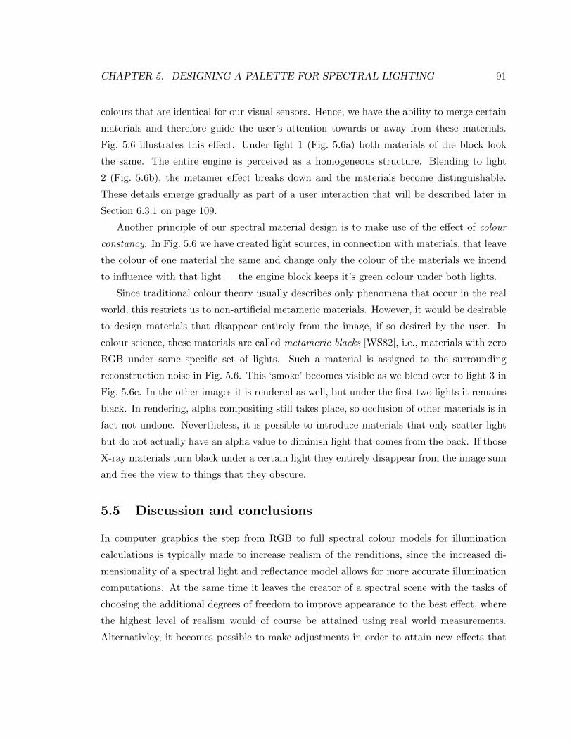
CHAPTER 5. DESIGNING A PALETTE FOR SPECTRAL LIGHTING 91
colours that are identical for our visual sensors. Hence, we have the ability to merge certain
materials and therefore guide the user’s attention towards or away from these materials.
Fig. 5.6 illustrates this effect. Under light 1 (Fig. 5.6a) both materials of the block look
the same. The entire engine is perceived as a homogeneous structure. Blending to light
2 (Fig. 5.6b), the metamer effect breaks down and the materials become distinguishable.
These details emerge gradually as part of a user interaction that will be described later in
Section 6.3.1 on page 109.
Another principle of our spectral material design is to make use of the effect of colour
constancy. In Fig. 5.6 we have created light sources, in connection with materials, that leave
the colour of one material the same and change only the colour of the materials we intend
to influence with that light — the engine block keeps it’s green colour under both lights.
Since traditional colour theory usually describes only phenomena that occur in the real
world, this restricts us to non-artificial metameric materials. However, it would be desirable
to design materials that disappear entirely from the image, if so desired by the user. In
colour science, these materials are called metameric blacks [WS82], i.e., materials with zero
RGB under some specific set of lights. Such a material is assigned to the surrounding
reconstruction noise in Fig. 5.6. This ‘smoke’ becomes visible as we blend over to light 3 in
Fig. 5.6c. In the other images it is rendered as well, but under the first two lights it remains
black. In rendering, alpha compositing still takes place, so occlusion of other materials is in
fact not undone. Nevertheless, it is possible to introduce materials that only scatter light
but do not actually have an alpha value to diminish light that comes from the back. If those
X-ray materials turn black under a certain light they entirely disappear from the image sum
and free the view to things that they obscure.
5.5 Discussion and conclusions
In computer graphics the step from RGB to full spectral colour models for illumination
calculations is typically made to increase realism of the renditions, since the increased di-
mensionality of a spectral light and reflectance model allows for more accurate illumination
computations. At the same time it leaves the creator of a spectral scene with the tasks of
choosing the additional degrees of freedom to improve appearance to the best effect, where
the highest level of realism would of course be attained using real world measurements.
Alternativley, it becomes possible to make adjustments in order to attain new effects that

CHAPTER 5. DESIGNING A PALETTE FOR SPECTRAL LIGHTING 92
are specific to spectra. Since the colour appearance of a material is dependent on the illu-
mination and typically differs under varying illumination, the key idea pursued here was to
conduct a combined design for pairs of reflectances and lights.
The example palette in Fig. 5.1 showed a simple setup, using metamerism under one light,
that breaks apart into distinguishable colours under a different light. This palette is used
in a spectral texture of Fig. 5.5 to illustrate how non-/metamerism under specific lighting
can be used to reveal texture details selectively via lighting change. A possible extension to
such a setup would be a dynamic scene in which the user introduces the metamer-breaking
light via a flashlight. In that case, the flashlight would become a metaphor for revealing
additional detail in the scene.
The same idea of merging and splitting metamers may be applied hierarchically to a
palette, in Fig. 5.2. The idea here is that under one illumination (daylight) the entire
scene has a homogeneous appearance. Under additional ‘split’ lights there are 3 and then
5 classes distinguishable leading to different levels of discernability, e.g., in a rendition of a
map. Using this in a spectral texture similar to Fig. 5.5 forms a new way to scale visual
complexity by selectively introducing additional texture detail.
Also, controlling the lighting in the spectrum design addresses a problem pointed out by
Smits [Smi99] that some colours can only be modeled with physically implausible reflectances
that have magnitudes larger than 1. However, when considering colour as perceived from
an image one does not deal with reflectances, but rather reflected spectra, which involve
the multiplication of a light source spectrum. By considering colours for light-reflectance
combinations, the [0,1] bounds for reflectances can be maintained by scaling up the intensity
of the light sources. One way to obtain a suitable scaling is to initially produce reflectances
without upper bound. If their maximum magnitude is above 1, we may scale up all lights
by that magnitude value and repeat the design with a forced upper bound of 1 for the
reflectances.
The design errors discussed in § 5.4.2 were shown to depend on the number of constraints
and also on enforcement of positivity. In response to this situation, the user has to make
a decision. Firstly, the user could adjust the importance weights to drive the compromise
of conflicting criteria, e.g., favoring the colour combinations that have the highest visible
errors or that matter most to the final result. This in particular applies to the metamers,
that are supposed to look exactly the same. To achieve this we set the importance of the
metameric colour patches 4 or 10 times higher than that of the remaining ones. Another
CHAPTER 5. DESIGNING A PALETTE FOR SPECTRAL LIGHTING 93
solution are ‘free’ colours, since these allow us to choose a ‘natural’ metameric colour that
is easiest to fulfill in concert with the other given colour conditions.
As an additional option, in case precise colour fulfillment is very important, the positivity
constraint could be dropped to allow spectra with negative components. As a result, the
optimization may more likely fulfill the given criteria without any error (see Fig. 5.3c). The
same figure also indicates that choosing an even higher dimensional spectral model is yet
another possibility for satisfying more constraints.
This kind of iterative design process of adjusting criteria to what is possible has not
been performed in our automatic evaluation, but is feasible in practice. An interactive
‘live’ update feature of our Java implementation was found to be helpful in this regard. It
performs the re-design (constructing and solving the criteria matrix) in a background thread
whenever changes are made. This immediate feedback allows the user to adjust conflicting
colours or constraints the moment they are introduced.
5.5.1 Future directions
The design has so far only considered colours of single illuminants combined with single
reflectances. In rendering practice, one may also be interested in mixtures of different
illuminants as well as materials of combined reflectances. While the light source mixture
would be linear due to additive superposition of the electromagnetic field, the same may
not hold for reflectances of mixed materials.
More advanced illumination models could be taken into account. For instance a bi-
reflectivity matrix relating illuminating wavelengths to re-emitted wavelengths [DCWP02]
could be used to model fluorescence. In fact, one could readily apply such a matrix, replacing
diag( ~E) in Eq. 5.8 and design a light ~E to produce a given colour on a fluorescent surface.
A feature similar to the free colour approach that creates two or more colours that are
as distinct as possible rather than equal could be useful. In that case, it might be helpful
to switch to a more perceptually uniform colour space. A linear approximation to CIELAB
[SHT97] could be of use here. Work in such a direction should also consider perceptual
issues of palette creation [HB03].
Just like physical simulation can replace manual geometrical modeling, e.g., for cloth or
water surfaces employing spectral rendering could achieve the same for lighting and colour
appearance. That is, with sets of materials designed to produce a well balanced and distinct
appearance under various lights. Instead of changing the palette to create a different mood
CHAPTER 5. DESIGNING A PALETTE FOR SPECTRAL LIGHTING 94
the change would be implicit under a different light.
With a proper paint mixture model one could look for feasible spectra that could be
mixed from paints or in combination with other base materials, such as metals or textiles
or even skin as in the case of face masks and make-up.
All our examples are given in the context of image synthesis. But a method to construct
spectra might also be used for reconstruction of spectra in a computer vision setting, e.g.,
using multiple images of the same scene taken under different colour filters or different
controlled illumination. Here, each colour filter would give rise to a distinct spectrum to
camera RGB transformation matrix that takes the effect of the filter into account via a
pre-multiplied diagonal matrix containing the filter absorbance spectrum. The optimization
of the design method could then reconstruct a spectrum that simultaneously fulfills the
different recorded RGB values of a given image pixel under the respective colour filtered
transformation matrices.
5.5.2 Conclusions
Even though spectral rendering is fairly easy to implement, it is still not widely used.
Performance issues are only partly a reason. In fact, due to cache coherency and with
cheap component-wise illumination calculations, the drop in performance is not significant.
Rather, we felt that it is the lack of spectral materials and the difficulty of reusing existing
RGB setups and textures within a spectral setup that have posed an obstacle to users.
To close this crucial gap in the design pipeline, we have devised a spectral palette tool
that allows the user to create a set of lights and reflectances such that different parts of a
rendering can be enhanced, or be made to disappear, in real time and interactively. We
formulated the design process as a least squares problem, yielding global minimization of
the criteria. The design scheme and optimization is novel in both graphics as well as in
colour science. The resulting set of spectra and colours have utility in the visualization
of volume data, but their usefulness is not restricted to this arena or to surface graphics.
In fact, with the liberty to inject actual physical spectra for any of the components, one
may design appropriate lights to attain specific perceived colours when viewing real physical
subjects.
Chapter 6
Interactive parameter space partitioning
Computational power today enables researchers to build and study algorithmic models that
may involve large numbers of variables and complex relations among them. The gist of
Chapter 1 was that in order to draw any practically relevant conclusions from a simulation,
it remains crucial to ensure a close correspondence between formal model and the real-world
system under scrutiny.
A possible step to achieve this correspondence is to match model output with measured
field data. However, in early modelling stages such data may not be available and a law-
driven approach has to be chosen. Beyond that, even after fitting given observations there
may still be free model parameters that can be controlled to adjust the behaviour of the
computer simulation. This can happen, if the expressive power of the model exceeds the
number of available measurements, or if the measurements are so noisy that several different
model instances are equally acceptable. To formally address this case, it is possible to
introduce additional regularizing criteria that a solution has to fulfill. This was, for instance,
done in the context of our spectral palette design in Equation 5.13 on page 82 by minimizing
the curvature of the generated distribution functions. Instead of using numerical criteria,
the user could be given a method to interactively tune free parameters of the model to favour
more plausible solutions that match prior experience. In such a case, a domain expert could
be involved to interactively tune parameters of the model or to prescribe ranges that favour
solutions that match prior experience, theoretical insight, or intuition.
Towards that goal, we recognize that the optimization of parameters for some notion
of performance is distinct from the objective to discover regions in parameter space that
exhibit qualitatively different system behaviour, such as fluid vs. gaseous state, or formation
95
CHAPTER 6. INTERACTIVE PARAMETER SPACE PARTITIONING 96
of various movement patterns in a swarm simulation. Optimization is one focus of statistical
methods in experimental design and has great potential for integration with visual tools, as
for instance demonstrated recently by Torsney-Weir et al. [TWSM+11].
The focus of this chapter is on the latter aspect of qualitative discovery. This can
support the understanding of the studied system, strengthen confidence in the suitability of
the modelling mechanisms and, thus, become a substantial aid in the research process.
In the context of modelling this is a novel viewpoint, since typical approaches calibrate
one best version of the model and then study how it behaves. To put regional parameter
space exploration into practice, a number of challenges have to be overcome. To identify and
address those, we (a) performed a field analysis of three application domains and derived
a list of requirements in Section 1.2, (b) present paraglide, a system that addresses these
requirements with a set of interaction and visualization techniques novel for this kind of
application area, (c) conducted a longitudinal field evaluation of paraglide showing practical
benefits. In summary, paraglide sets out to make the following contributions to computational
modelling:
• Parameter region construction is promoted as a separate user interaction step dur-
ing experimental design. This allows to address different efficiency issues of multi-
dimensional sampling.
• A common step in explorative hypothesis formation is the construction of additional
dependent feature variables and goal functions. Paraglide facilitates this with inter-
preter based back-ends. Also, this seamlessly integrates model code from sources such
as MATLAB, R, or Python.
• Qualitatively distinct solutions are identified and the parameter space of the model is
partitioned into the corresponding regions. This allows to visually derive global state-
ments about the sensitivity of the model to parameter changes, which traditionally is
studied locally.
6.1 Background
Research that is related to visual analysis of multi-dimensional data has been discussed in
Section 2.4 and specifically Section 2.4.4. Hence, the following review can focus specifically
CHAPTER 6. INTERACTIVE PARAMETER SPACE PARTITIONING 97
on user interfaces that adress some aspects of interactive parameter adjustment of compu-
tational models. Methods that are more specific to the design of particular components of
paraglide will be discussed in the respective sections of Section 6.2.
6.1.1 Interactive parameter adjustment in computer experiments
Computational steering systems focus on adjustment of parameters during execution of
time-dependent simulations [MvWvL99]. Since our users do not modify parameters during
the run of a simulation, our problem setting is different from classical steering in that we do
not need to handle live updates of variables that are shared between simultaneously running
modules. However, there is enough similarity to benefit from a comparison.
Wijk et al. [vWVLM97] performed an evaluation of their computational steering en-
vironment (CSE) and recognized major uses for debugging, presentation, and assistance
in technical discussions that progress faster when “What if?” questions can be answered
immediately. A follow-up survey by Mulder et al. [MvWvL99] identified further uses for
model exploration, algorithm experimentation, and performance optimization. While these
systems inspire numerous design decisions, the specific requirements for efficient regional
sampling and an easy integration of end-user codes for simulation and derived variable
computation are either not fulfilled or could be improved.
Berger et al. [BPFG11] discuss a system to visualize engineering and design options
in the neighbourhood around an optimal configuration of a computer simulation. Based
on a continuous function abstraction they provide a local analysis method that benefits
domain experts. In order to not get stuck in local maxima, optimization methods usually
benefit from an additional global perspective on the problem domain. The qualitative
decomposition pointed out in the cases of Section 1.2 and pursued in the following provides
such a complementary view.
The challenge of devising a user interaction for sample construction has recently been
taken on in the Paranorama system of Pretorius et al. [PBCR11]. Their users can specify
different ranges of interest for individual variables along with the number of requested
distinct values per range. The sample points are then constructed via a Cartesian product
of the value sets. Integrating this method into an image segmentation system, received
positive feedback from users. However, combining many value ranges with this method may
result in large sampling costs. Beyond numerical arguments, also screen space real estate
is used up more quickly when viewing data sets with large numbers of variables, and a
CHAPTER 6. INTERACTIVE PARAMETER SPACE PARTITIONING 98
significantly increased cognitive cost arises when investigating and interpreting the effects
of many factors on possibly multiple responses. Due to their significant impact on sampling
and processing costs, Section 6.2.3 will give careful consideration to the number of involved
variables and the volume of the region of interest.
6.1.2 Parameter space partitioning
The computational model analysis cases of Section 1.2 all benefit from an overview of regions
of distinct system behaviour marked out in their input parameter space (R5 of Table 1.1
on page 12). So far, there is no prior research in the visualization community that provides
such a representation. After considering different names for the method, such as parameter
space segmentation, clustering, or partitioning, it is the latter term that relates us to two
prior contributions from an old and a recent member of the sciences, namely physics and
psychology.
Bhatt and Koechling [BK95] study the behaviour during impact of two solid bodies with
finite friction and restitution, which results in a tangential sliding velocity that continuously
changes direction after impact. The problem is characterized by 9 parameters, three for
the impulse direction of the impacting body and six for its rotational moment of inertia
tensor. The first step of their analysis determines a reduced set of three dimensionless
parameters that completely define the tangential flow of sliding velocities. An important
observation is that the qualitative behaviour of the flow is characterized by 2 or 4 solution
curves of invariant direction, as well as the critical points and sign changes of the velocity
along these straight lines. This results in 4 main cases with up to 3 sub-cases each. An
implicit expression of the boundary between the cases is derived that is quartic in terms
of the 3 dimensionless parameters. By fixing one parameter and showing slices through
this boundary, the enclosed regions can be visually distinguished and are labelled with the
different cases they represent. This provides a comprehensive overview of all possible sliding
behaviour. While providing a sophisticated algebraic analysis of a specific phenomenon, their
discussion does not deal with numeric aspects involved of general computational models.
Pitt et al. [PKNM06] also promote parameter space partitioning with an example anal-
ysis of a model to predict, whether visual stimuli are recognized as words or non-words. In
their overview of analysis techniques, they distinguish two axes that separate quantitative
from qualitative and local from global techniques. In this view, partitioning is a global,
qualitative method, and sensitivity analysis a case of more local, quantitative inspection.
CHAPTER 6. INTERACTIVE PARAMETER SPACE PARTITIONING 99
Their method proceeds from a notion of equivalence among model configurations and a
set of valid seed configuration points. The regions around these points are sampled using a
Metropolis-Hastings algorithm with uniform target distribution. Rejected points have fallen
into non-equivalent, adjacent regions and are explored subsequently.
An important point made by Pitt et al. is to also address the need to improve the user’s
confidence in the plausibility of a given model. The studies they present are supported
by showing the variety of qualitatively distinct model behaviour. However, a discussion of
suitable analysis system design and considerations of required user interactions are not the
focus of their exposition.
6.1.3 Unfulfilled design requirements
Methods to visually inspect multi-variate point distributions (to address R3a of Table 1.1)
are available in several of the frameworks listed earlier in Sections 2.4.4 and 6.1.1. However,
the required capability to also generate data points (R2a) or to add derived dimensions (R4a)
is missing from most systems that are mainly geared towards visualization of a static data
set. Systems for experimental design, on the other hand, take care of the sampling require-
ments (R2a), but often lack interactive, visual methods to solicit required user input (R2).
Computational steering systems combine sampling and visualization, but specifically focus
on live-adjustments to parameters of a simulation that evolves over time. Their focus is
often on some sort of interactive investigation, which could benefit from further support for
broader state discovery (R5).
6.2 Design of the paraglide system
We will now discuss aspects of the design of paraglide, giving individual consideration to the
graphical user interface (GUI), the software system, and choices of algorithms or methods
for particular tasks. Paraglide was developed in a user-centered design process with five users,
one or two from each domain. We met with our participants in person covering longitudinal
time ranges of four years (fuel cell engineering), two years (mathematical modelling), with
monthly meetings, and five months (image segmentation) with weekly meetings. In these
meetings we discussed design mockups and prototypes, observed our users working with
paraglide, and gathered formative feedback in terms of usability and feature requests that
we used to improve paraglide’s design. In addition, these meetings contributed to refining
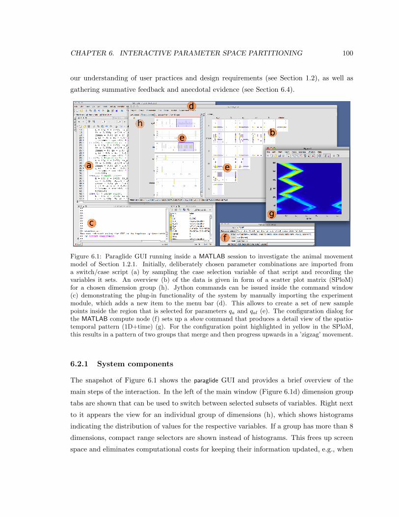
CHAPTER 6. INTERACTIVE PARAMETER SPACE PARTITIONING 100
our understanding of user practices and design requirements (see Section 1.2), as well as
gathering summative feedback and anecdotal evidence (see Section 6.4).
a
c
b
d
e
f
g
e
h
Figure 6.1: Paraglide GUI running inside a MATLAB session to investigate the animal movementmodel of Section 1.2.1. Initially, deliberately chosen parameter combinations are imported froma switch/case script (a) by sampling the case selection variable of that script and recording thevariables it sets. An overview (b) of the data is given in form of a scatter plot matrix (SPloM)for a chosen dimension group (h). Jython commands can be issued inside the command window(c) demonstrating the plug-in functionality of the system by manually importing the experimentmodule, which adds a new item to the menu bar (d). This allows to create a set of new samplepoints inside the region that is selected for parameters qa and qal (e). The configuration dialog forthe MATLAB compute node (f) sets up a show command that produces a detail view of the spatio-temporal pattern (1D+time) (g). For the configuration point highlighted in yellow in the SPloM,this results in a pattern of two groups that merge and then progress upwards in a ’zigzag’ movement.
6.2.1 System components
The snapshot of Figure 6.1 shows the paraglide GUI and provides a brief overview of the
main steps of the interaction. In the left of the main window (Figure 6.1d) dimension group
tabs are shown that can be used to switch between selected subsets of variables. Right next
to it appears the view for an individual group of dimensions (h), which shows histograms
indicating the distribution of values for the respective variables. If a group has more than 8
dimensions, compact range selectors are shown instead of histograms. This frees up screen
space and eliminates computational costs for keeping their information updated, e.g., when
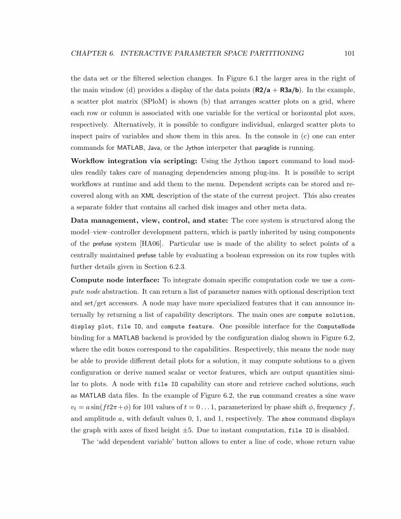
CHAPTER 6. INTERACTIVE PARAMETER SPACE PARTITIONING 101
the data set or the filtered selection changes. In Figure 6.1 the larger area in the right of
the main window (d) provides a display of the data points (R2/a + R3a/b). In the example,
a scatter plot matrix (SPloM) is shown (b) that arranges scatter plots on a grid, where
each row or column is associated with one variable for the vertical or horizontal plot axes,
respectively. Alternatively, it is possible to configure individual, enlarged scatter plots to
inspect pairs of variables and show them in this area. In the console in (c) one can enter
commands for MATLAB, Java, or the Jython interpeter that paraglide is running.
Workflow integration via scripting: Using the Jython import command to load mod-
ules readily takes care of managing dependencies among plug-ins. It is possible to script
workflows at runtime and add them to the menu. Dependent scripts can be stored and re-
covered along with an XML description of the state of the current project. This also creates
a separate folder that contains all cached disk images and other meta data.
Data management, view, control, and state: The core system is structured along the
model–view–controller development pattern, which is partly inherited by using components
of the prefuse system [HA06]. Particular use is made of the ability to select points of a
centrally maintained prefuse table by evaluating a boolean expression on its row tuples with
further details given in Section 6.2.3.
Compute node interface: To integrate domain specific computation code we use a com-
pute node abstraction. It can return a list of parameter names with optional description text
and set/get accessors. A node may have more specialized features that it can announce in-
ternally by returning a list of capability descriptors. The main ones are compute solution,
display plot, file IO, and compute feature. One possible interface for the ComputeNode
binding for a MATLAB backend is provided by the configuration dialog shown in Figure 6.2,
where the edit boxes correspond to the capabilities. Respectively, this means the node may
be able to provide different detail plots for a solution, it may compute solutions to a given
configuration or derive named scalar or vector features, which are output quantities simi-
lar to plots. A node with file IO capability can store and retrieve cached solutions, such
as MATLAB data files. In the example of Figure 6.2, the run command creates a sine wave
vt = a sin(ft2π+φ) for 101 values of t = 0 . . . 1, parameterized by phase shift φ, frequency f ,
and amplitude a, with default values 0, 1, and 1, respectively. The show command displays
the graph with axes of fixed height ±5. Due to instant computation, file IO is disabled.
The ‘add dependent variable’ button allows to enter a line of code, whose return value
CHAPTER 6. INTERACTIVE PARAMETER SPACE PARTITIONING 102
Figure 6.2: Dialog to set up a MATLAB compute node
is assigned to a variable of chosen name. This implements the derived variables yi = g(y)
described in Section 1.4 and serves requirements R4/a. If a scalar is returned, it can be
shown in the SPloM view along with the input variables. It is also possible to return vector
features that may not be shown directly, but can be used to compute similarity or distance
matrices, or to determine adjacency information. Methods to derive further embedding
coordinates from this information are discussed in Section 6.2.4. The example in Figure 6.2
picks out the deflection of the oscillation at time t = 0 (v0) and half way into the interval
(v 12). When inspecting these two local features, it becomes apparent that v0 depends on
a and φ only, where v 12
is influenced by all three parameters. In this simple setting, it is
possible to make this observation by thinking about the equation given for v, as well as by
studying the scatter plots of input/output variable combinations. For the latter method,
however, we would first need to create a data set of tuples (a, f, φ, v0, v 12).
With a readily configured connection to the simulation back-end, paraglide has a notion
of the input parameter space Rn as well as the output space Rr of the simulation code.
Initially, however, there may only be a single point of default values present, around which
it is possible to expand the data set. To generate additional points it is possible to use some
of the methods discussed in Section 2.3.2. While paraglide does not require to start with a
given data set, the following discussion of system components will assume that an initial set
of points already exists.
6.2.2 Browsing computed data
This stage provides the user with an overview of the data points as they distribute over
input, output, and derived dimensions.
CHAPTER 6. INTERACTIVE PARAMETER SPACE PARTITIONING 103
6.2.2.1 Viewing multi-dimensional data spaces
To address requirements R3a/b, we provide multiple simultaneous plots that give different
views of the same data table and are linked to display a common focus point, highlight,
or selection region. The subspaces that can be visualized that way range from multi- to
0-dimensional, to allow the user to relate overview of the whole distribution and detail plots
that represent a single point. We also provide techniques to view 2D subspaces, such as
scatter plots that allow for pair-wise inspection of relationships among variables, and 1D
projections of the marginal densities that can be shown in form of histograms.
There are many more possible techniques for multi-variate multi-field data visualization,
such as parallel coordinates, star plots, biplots, glyph-based visual encodings, or scatter plots
arranged in a matrix or table layout, with discussions of pros and cons provided in various
surveys [Hol06, FdOL03]. Implementations of these techniques are either contained directly
in paraglide or are available via export to MATLAB, R, or protovis.
6.2.2.2 Grouping dimensions
As mentioned at the outset of this chapter, the increased number of variables involved with
modern simulation codes poses a challenge for their cognitive and numerical analysis. The
visual complexity rises and makes data plots more difficult to interpret. The strategy of
combining multiple views has its limits in screen space, as well as perceptual and cognitive
handling. A possible remedy to this problem could be a) indirect visualization of fitted
reduced dimensional models [Hol06], or b) to divide the overall number of dimensions into
groups for more focussed inspection.
Grouping simplifies complexity and can be based on statistical or structural information.
Research on grouping of variables may consider dimension reduction and feature selection.
To allow the user to express semantic information, we provide an interface to construct or
modify a dimension group that simply consists of check boxes that indicate group member-
ship for each variable. During browsing, only dimensions of the currently selected group
are shown, which reduces the required screen space. While automatic assistance in forming
these groups is imaginable, our current approach of manual selection proved sufficient in all
use cases.

CHAPTER 6. INTERACTIVE PARAMETER SPACE PARTITIONING 104
6.2.2.3 Scatterplots for points in continuous data spaces
The possible use of scatterplots in the context of sensitivity analysis (R7) is pointed out by
Saltelli et al. [SRA+08, Sec. 1.2.3].
Conventional scatterplots show points directly. However, for the computer simulations
under consideration, there is an underlying continuous phenomenon. This means that a)
interpolated density distributions could be reconstructed and displayed, b) input and output
dimensions (or variables) with clear dependency relationships can be distinguished, and c)
descriptions of continuous region in data space can be visualized.
A classical technique to realize (a) is kernel density estimation, where instead of drawing
a dot for each point, a kernel that smoothly decays with increasing distance from the point
is additively rendered into the screen plane. In the language of direct volume visualization
this amounts to splatting with additive, X-ray-type compositing. A typical issue with this
approach is the proper choice of kernel diameter for proper reconstruction of multi-modal
density distributions.
Being able to separately consider input and output dimensions (b), enables an elegant
way to address this issue in scatterplots of the output. For a generated sampling pattern,
point adjacencies in the input space are known or can be obtained by constructing a Delau-
nay mesh that connects Voronoi relevant neighbours. The faces of this mesh are simplices
in the typical case or bounded cells in general. To reconstruct the projected continuous
density for a scatterplot of output dimensions, it is possible to project the cells between
the points, instead of kernels representing the points themselves [NH06, ST90]. For further
background see Section 2.4.2.
The accuracy of a reconstructed density distribution varies based on distance from the
given points. This introduces an additional challenge to continuous visualizations that
direct point drawings do not have, since a notion of uncertainty is readily perceivable as
gaps between points. This is one reason, why continuous density plots are not used in
paraglide, and we instead opt for a more easily interpretable direct point display.
Apart from a density distribution, it is possible to visualize other continuous objects
that live in the same space along with the data points, as hinted earlier in point (c). In
general, this could ask for a direct visualization of scalar functions over a continuous domain.
More specifically, the construct required to address the presented use cases are 0, 1-valued
indicator functions that describe a continuous selection region.
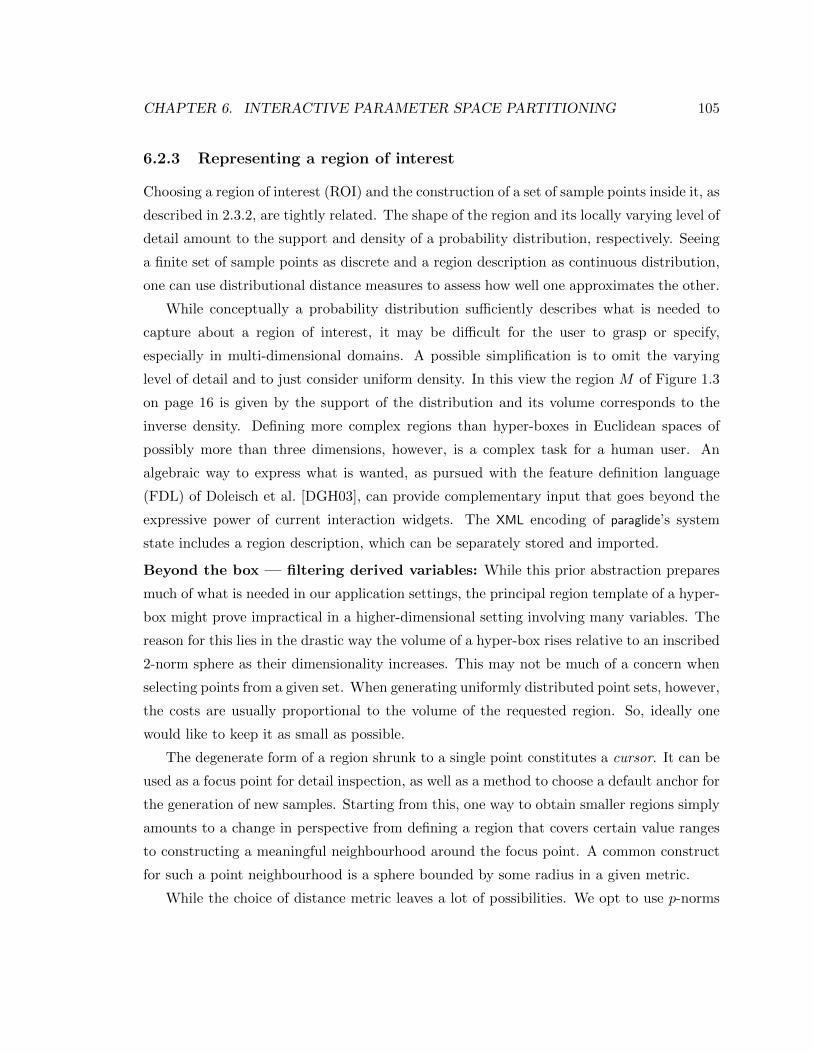
CHAPTER 6. INTERACTIVE PARAMETER SPACE PARTITIONING 105
6.2.3 Representing a region of interest
Choosing a region of interest (ROI) and the construction of a set of sample points inside it, as
described in 2.3.2, are tightly related. The shape of the region and its locally varying level of
detail amount to the support and density of a probability distribution, respectively. Seeing
a finite set of sample points as discrete and a region description as continuous distribution,
one can use distributional distance measures to assess how well one approximates the other.
While conceptually a probability distribution sufficiently describes what is needed to
capture about a region of interest, it may be difficult for the user to grasp or specify,
especially in multi-dimensional domains. A possible simplification is to omit the varying
level of detail and to just consider uniform density. In this view the region M of Figure 1.3
on page 16 is given by the support of the distribution and its volume corresponds to the
inverse density. Defining more complex regions than hyper-boxes in Euclidean spaces of
possibly more than three dimensions, however, is a complex task for a human user. An
algebraic way to express what is wanted, as pursued with the feature definition language
(FDL) of Doleisch et al. [DGH03], can provide complementary input that goes beyond the
expressive power of current interaction widgets. The XML encoding of paraglide’s system
state includes a region description, which can be separately stored and imported.
Beyond the box — filtering derived variables: While this prior abstraction prepares
much of what is needed in our application settings, the principal region template of a hyper-
box might prove impractical in a higher-dimensional setting involving many variables. The
reason for this lies in the drastic way the volume of a hyper-box rises relative to an inscribed
2-norm sphere as their dimensionality increases. This may not be much of a concern when
selecting points from a given set. When generating uniformly distributed point sets, however,
the costs are usually proportional to the volume of the requested region. So, ideally one
would like to keep it as small as possible.
The degenerate form of a region shrunk to a single point constitutes a cursor. It can be
used as a focus point for detail inspection, as well as a method to choose a default anchor for
the generation of new samples. Starting from this, one way to obtain smaller regions simply
amounts to a change in perspective from defining a region that covers certain value ranges
to constructing a meaningful neighbourhood around the focus point. A common construct
for such a point neighbourhood is a sphere bounded by some radius in a given metric.
While the choice of distance metric leaves a lot of possibilities. We opt to use p-norms
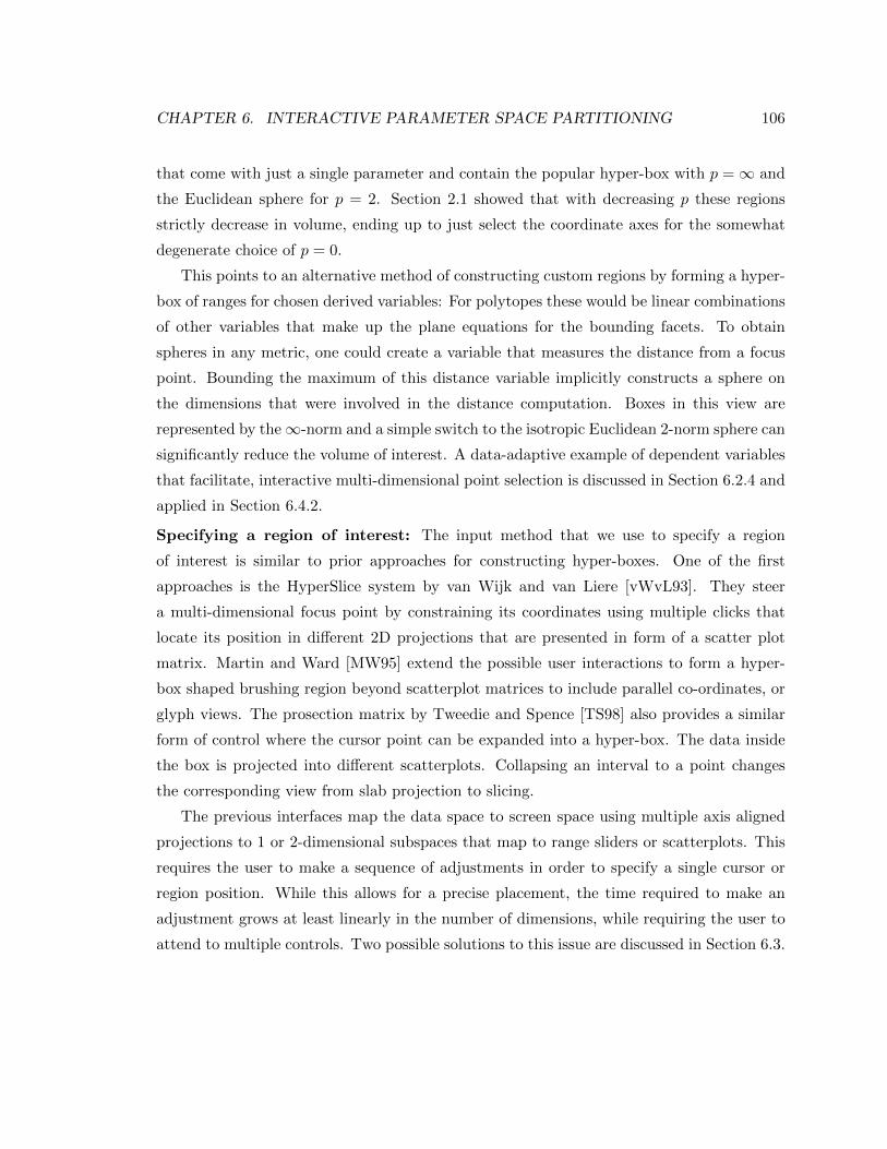
CHAPTER 6. INTERACTIVE PARAMETER SPACE PARTITIONING 106
that come with just a single parameter and contain the popular hyper-box with p =∞ and
the Euclidean sphere for p = 2. Section 2.1 showed that with decreasing p these regions
strictly decrease in volume, ending up to just select the coordinate axes for the somewhat
degenerate choice of p = 0.
This points to an alternative method of constructing custom regions by forming a hyper-
box of ranges for chosen derived variables: For polytopes these would be linear combinations
of other variables that make up the plane equations for the bounding facets. To obtain
spheres in any metric, one could create a variable that measures the distance from a focus
point. Bounding the maximum of this distance variable implicitly constructs a sphere on
the dimensions that were involved in the distance computation. Boxes in this view are
represented by the∞-norm and a simple switch to the isotropic Euclidean 2-norm sphere can
significantly reduce the volume of interest. A data-adaptive example of dependent variables
that facilitate, interactive multi-dimensional point selection is discussed in Section 6.2.4 and
applied in Section 6.4.2.
Specifying a region of interest: The input method that we use to specify a region
of interest is similar to prior approaches for constructing hyper-boxes. One of the first
approaches is the HyperSlice system by van Wijk and van Liere [vWvL93]. They steer
a multi-dimensional focus point by constraining its coordinates using multiple clicks that
locate its position in different 2D projections that are presented in form of a scatter plot
matrix. Martin and Ward [MW95] extend the possible user interactions to form a hyper-
box shaped brushing region beyond scatterplot matrices to include parallel co-ordinates, or
glyph views. The prosection matrix by Tweedie and Spence [TS98] also provides a similar
form of control where the cursor point can be expanded into a hyper-box. The data inside
the box is projected into different scatterplots. Collapsing an interval to a point changes
the corresponding view from slab projection to slicing.
The previous interfaces map the data space to screen space using multiple axis aligned
projections to 1 or 2-dimensional subspaces that map to range sliders or scatterplots. This
requires the user to make a sequence of adjustments in order to specify a single cursor or
region position. While this allows for a precise placement, the time required to make an
adjustment grows at least linearly in the number of dimensions, while requiring the user to
attend to multiple controls. Two possible solutions to this issue are discussed in Section 6.3.
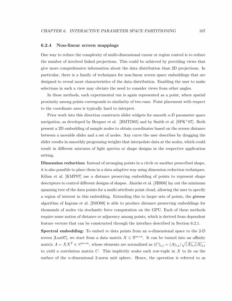
CHAPTER 6. INTERACTIVE PARAMETER SPACE PARTITIONING 107
6.2.4 Non-linear screen mappings
One way to reduce the complexity of multi-dimensional cursor or region control is to reduce
the number of involved linked projections. This could be achieved by providing views that
give more comprehensive information about the data distribution than 2D projections. In
particular, there is a family of techniques for non-linear screen space embeddings that are
designed to reveal most characteristics of the data distribution. Enabling the user to make
selections in such a view may obviate the need to consider views from other angles.
In these methods, each experimental run is again represented as a point, where spatial
proximity among points corresponds to similarity of two runs. Point placement with respect
to the coordinate axes is typically hard to interpret.
Prior work into this direction constructs slider widgets for smooth n-D parameter space
navigation, as developed by Bergner et al. [BMTD05] and by Smith et al. [SPK+07]. Both
present a 2D embedding of sample nodes to obtain coordinates based on the screen distance
between a movable slider and a set of nodes. Any curve the user describes by dragging the
slider results in smoothly progressing weights that interpolate data at the nodes, which could
result in different mixtures of light spectra or shape designs in the respective application
setting.
Dimension reduction: Instead of arranging points in a circle or another prescribed shape,
it is also possible to place them in a data adaptive way using dimension reduction techniques.
Kilian et al. [KMP07] use a distance preserving embedding of points to represent shape
descriptors to control different designs of shapes. Janicke et al. [JBS08] lay out the minimum
spanning tree of the data points for a multi-attribute point cloud, allowing the user to specify
a region of interest in this embedding. Extending this to larger sets of points, the glimmer
algorithm of Ingram et al. [IMO09] is able to produce distance preserving embeddings for
thousands of nodes via stochastic force computation on the GPU. Each of these methods
require some notion of distance or adjacency among points, which is derived from dependent
feature vectors that can be constructed through the interface described in Section 6.2.1.
Spectral embedding: To embed m data points from an n-dimensional space to the 2-D
screen [Lux07], we start from a data matrix X ∈ Rm×n. It can be turned into an affinity
matrix A = XXT ∈ Rm×m, whose elements are normalized as (C)i,j = (A)i,j/√
(A)i,i(A)j,j
to yield a correlation matrix C. This implicitly scales each row-tuple in X to lie on the
surface of the n-dimensional 2-norm unit sphere. Hence, the operation is referred to as
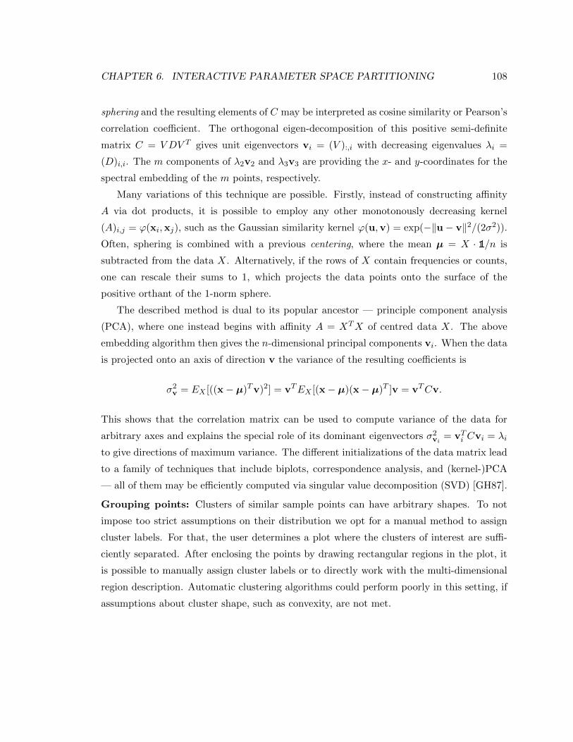
CHAPTER 6. INTERACTIVE PARAMETER SPACE PARTITIONING 108
sphering and the resulting elements of C may be interpreted as cosine similarity or Pearson’s
correlation coefficient. The orthogonal eigen-decomposition of this positive semi-definite
matrix C = V DV T gives unit eigenvectors vi = (V ):,i with decreasing eigenvalues λi =
(D)i,i. The m components of λ2v2 and λ3v3 are providing the x- and y-coordinates for the
spectral embedding of the m points, respectively.
Many variations of this technique are possible. Firstly, instead of constructing affinity
A via dot products, it is possible to employ any other monotonously decreasing kernel
(A)i,j = ϕ(xi,xj), such as the Gaussian similarity kernel ϕ(u,v) = exp(−‖u− v‖2/(2σ2)).
Often, sphering is combined with a previous centering, where the mean µ = X · 1/n is
subtracted from the data X. Alternatively, if the rows of X contain frequencies or counts,
one can rescale their sums to 1, which projects the data points onto the surface of the
positive orthant of the 1-norm sphere.
The described method is dual to its popular ancestor — principle component analysis
(PCA), where one instead begins with affinity A = XTX of centred data X. The above
embedding algorithm then gives the n-dimensional principal components vi. When the data
is projected onto an axis of direction v the variance of the resulting coefficients is
σ2v = EX [((x− µ)Tv)2] = vTEX [(x− µ)(x− µ)T ]v = vTCv.
This shows that the correlation matrix can be used to compute variance of the data for
arbitrary axes and explains the special role of its dominant eigenvectors σ2vi = vTi Cvi = λi
to give directions of maximum variance. The different initializations of the data matrix lead
to a family of techniques that include biplots, correspondence analysis, and (kernel-)PCA
— all of them may be efficiently computed via singular value decomposition (SVD) [GH87].
Grouping points: Clusters of similar sample points can have arbitrary shapes. To not
impose too strict assumptions on their distribution we opt for a manual method to assign
cluster labels. For that, the user determines a plot where the clusters of interest are suffi-
ciently separated. After enclosing the points by drawing rectangular regions in the plot, it
is possible to manually assign cluster labels or to directly work with the multi-dimensional
region description. Automatic clustering algorithms could perform poorly in this setting, if
assumptions about cluster shape, such as convexity, are not met.
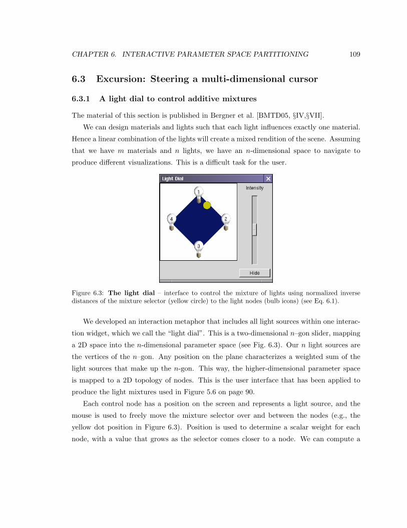
CHAPTER 6. INTERACTIVE PARAMETER SPACE PARTITIONING 109
6.3 Excursion: Steering a multi-dimensional cursor
6.3.1 A light dial to control additive mixtures
The material of this section is published in Bergner et al. [BMTD05, §IV,§VII].
We can design materials and lights such that each light influences exactly one material.
Hence a linear combination of the lights will create a mixed rendition of the scene. Assuming
that we have m materials and n lights, we have an n-dimensional space to navigate to
produce different visualizations. This is a difficult task for the user.
Figure 6.3: The light dial – interface to control the mixture of lights using normalized inversedistances of the mixture selector (yellow circle) to the light nodes (bulb icons) (see Eq. 6.1).
We developed an interaction metaphor that includes all light sources within one interac-
tion widget, which we call the “light dial”. This is a two-dimensional n–gon slider, mapping
a 2D space into the n-dimensional parameter space (see Fig. 6.3). Our n light sources are
the vertices of the n–gon. Any position on the plane characterizes a weighted sum of the
light sources that make up the n-gon. This way, the higher-dimensional parameter space
is mapped to a 2D topology of nodes. This is the user interface that has been applied to
produce the light mixtures used in Figure 5.6 on page 90.
Each control node has a position on the screen and represents a light source, and the
mouse is used to freely move the mixture selector over and between the nodes (e.g., the
yellow dot position in Figure 6.3). Position is used to determine a scalar weight for each
node, with a value that grows as the selector comes closer to a node. We can compute a

CHAPTER 6. INTERACTIVE PARAMETER SPACE PARTITIONING 110
weight Li(x) applied to the light for a selector position x in the following manner:
Li(x) =n∏
k=1, k 6=i
‖x− xk‖‖xi − xk‖
. (6.1)
To make the weights usable for combining light sources, we normalize the sum of all weights
Li to one and scale it with a separate intensity slider. When the position of the dot coincides
with the position of a light bulb in the widget, the influence of all other light sources is
eliminated. The influence of a source can be entirely removed by switching it off. Hence,
the light dial allows one to focus on the influence of a single light to the materials used in
the scene. It has not been designed to navigate the full n-D space at once. Instead, the
intention is to conveniently slide from one pure light to the next pure light.1 Additionally,
it is possible to correlate dimensions (making lights have similar intensity) by moving two
light bulbs closer to each other. This modifies the shape of the 2D mapping of the parameter
space and allows the user to reach new parameter constellations.
To summarize, our light dial implements three different interaction metaphors:
• move yellow dot (change weights by distance) — the object is weighted towards the
lights we want to see it under,
• move light nodes — group lights, or drag lights away to lower their influence (math-
ematically speaking: change shape of 2D mapping of higher-dimensional parameter
space, correlate dimensions by decreasing spatial distance in widget plane), and
• switch lights on/off (reducing dimensionality, comparable to taking a light node and
moving it far away; deactivation of the light allows it to keep its position in the
mapping plane.)
This makes the 2D dial a convenient interface to navigate through the colour schemes. The
light dial metaphor may be useful for other tasks, such as navigating between different points
of view, controlling alpha values of different segments, etc.
1Nevertheless, it is still possible to navigate the entire space of weight combinations. Imagine a concentricarrangement of the light bulbs around the light dot in the middle: all lights have the same weights. Now,a light bulb may be dragged instead of the dot, moved closer to or farther away from the center (where thedot is). Since only one distance is changing, it is possible to change only one weight. To actually have justone weight changing, the separate overall intensity slider would have to be moved correspondingly.
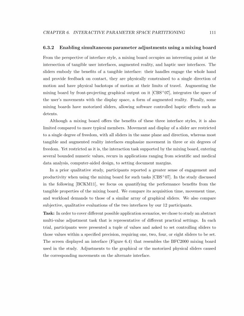
CHAPTER 6. INTERACTIVE PARAMETER SPACE PARTITIONING 111
6.3.2 Enabling simultaneous parameter adjustments using a mixing board
From the perspective of interface style, a mixing board occupies an interesting point at the
intersection of tangible user interfaces, augmented reality, and haptic user interfaces. The
sliders embody the benefits of a tangible interface: their handles engage the whole hand
and provide feedback on contact, they are physically constrained to a single direction of
motion and have physical backstops of motion at their limits of travel. Augmenting the
mixing board by front-projecting graphical output on it [CBS+07], integrates the space of
the user’s movements with the display space, a form of augmented reality. Finally, some
mixing boards have motorized sliders, allowing software controlled haptic effects such as
detents.
Although a mixing board offers the benefits of these three interface styles, it is also
limited compared to more typical members. Movement and display of a slider are restricted
to a single degree of freedom, with all sliders in the same plane and direction, whereas most
tangible and augmented reality interfaces emphasize movement in three or six degrees of
freedom. Yet restricted as it is, the interaction task supported by the mixing board, entering
several bounded numeric values, recurs in applications ranging from scientific and medical
data analysis, computer-aided design, to setting document margins.
In a prior qualitative study, participants reported a greater sense of engagement and
productivity when using the mixing board for such tasks [CBS+07]. In the study discussed
in the following [BCKM11], we focus on quantifying the performance benefits from the
tangible properties of the mixing board. We compare its acquisition time, movement time,
and workload demands to those of a similar array of graphical sliders. We also compare
subjective, qualitative evaluations of the two interfaces by our 12 participants.
Task: In order to cover different possible application scenarios, we chose to study an abstract
multi-value adjustment task that is representative of different practical settings. In each
trial, participants were presented a tuple of values and asked to set controlling sliders to
those values within a specified precision, requiring one, two, four, or eight sliders to be set.
The screen displayed an interface (Figure 6.4) that resembles the BFC2000 mixing board
used in the study. Adjustments to the graphical or the motorized physical sliders caused
the corresponding movements on the alternate interface.
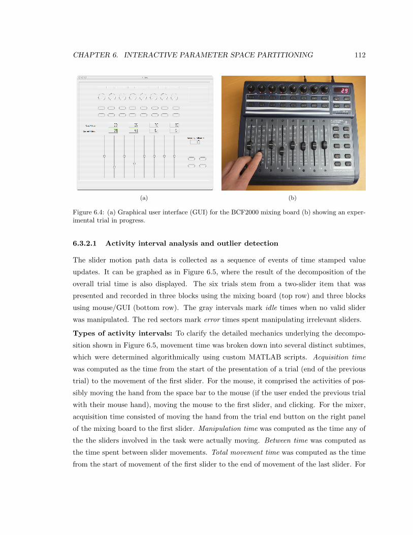
CHAPTER 6. INTERACTIVE PARAMETER SPACE PARTITIONING 112
(a) (b)
Figure 6.4: (a) Graphical user interface (GUI) for the BCF2000 mixing board (b) showing an exper-imental trial in progress.
6.3.2.1 Activity interval analysis and outlier detection
The slider motion path data is collected as a sequence of events of time stamped value
updates. It can be graphed as in Figure 6.5, where the result of the decomposition of the
overall trial time is also displayed. The six trials stem from a two-slider item that was
presented and recorded in three blocks using the mixing board (top row) and three blocks
using mouse/GUI (bottom row). The gray intervals mark idle times when no valid slider
was manipulated. The red sectors mark error times spent manipulating irrelevant sliders.
Types of activity intervals: To clarify the detailed mechanics underlying the decompo-
sition shown in Figure 6.5, movement time was broken down into several distinct subtimes,
which were determined algorithmically using custom MATLAB scripts. Acquisition time
was computed as the time from the start of the presentation of a trial (end of the previous
trial) to the movement of the first slider. For the mouse, it comprised the activities of pos-
sibly moving the hand from the space bar to the mouse (if the user ended the previous trial
with their mouse hand), moving the mouse to the first slider, and clicking. For the mixer,
acquisition time consisted of moving the hand from the trial end button on the right panel
of the mixing board to the first slider. Manipulation time was computed as the time any of
the the sliders involved in the task were actually moving. Between time was computed as
the time spent between slider movements. Total movement time was computed as the time
from the start of movement of the first slider to the end of movement of the last slider. For
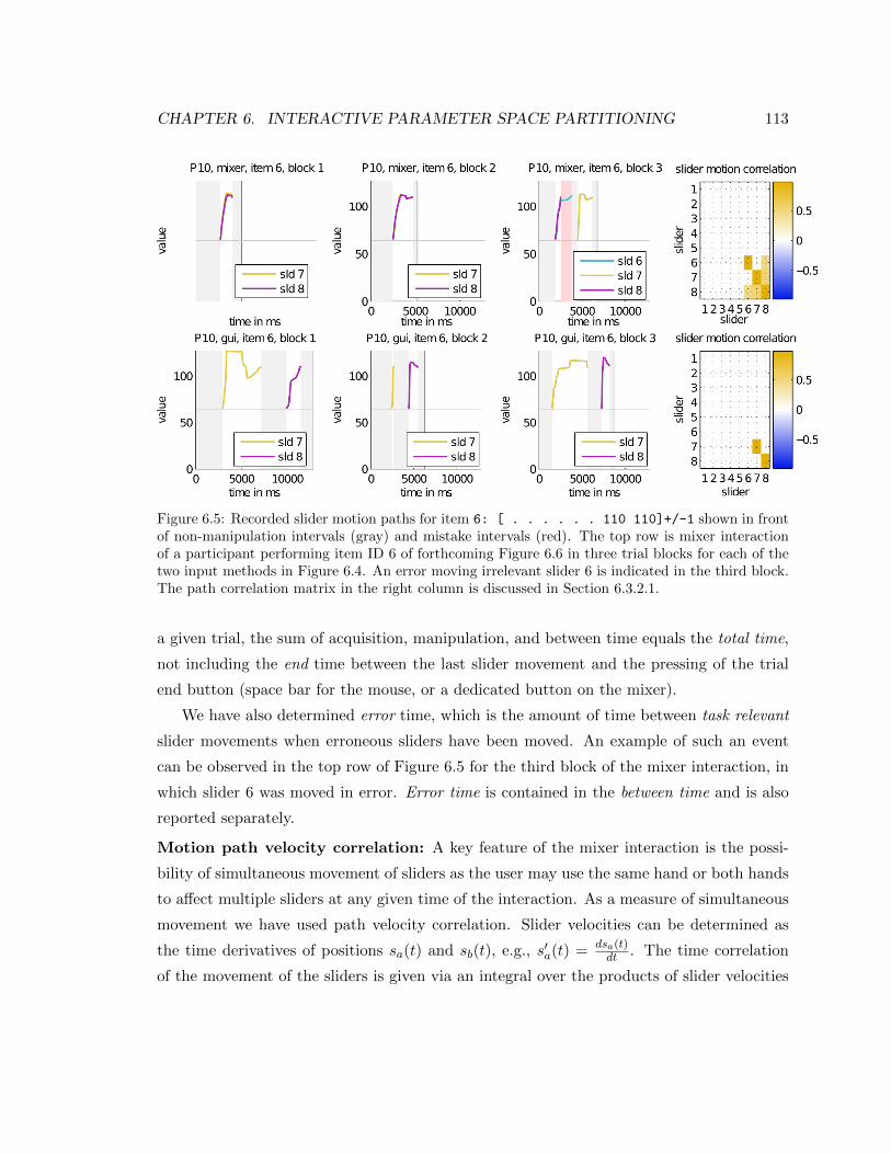
CHAPTER 6. INTERACTIVE PARAMETER SPACE PARTITIONING 113
Figure 6.5: Recorded slider motion paths for item 6: [ . . . . . . 110 110]+/-1 shown in frontof non-manipulation intervals (gray) and mistake intervals (red). The top row is mixer interactionof a participant performing item ID 6 of forthcoming Figure 6.6 in three trial blocks for each of thetwo input methods in Figure 6.4. An error moving irrelevant slider 6 is indicated in the third block.The path correlation matrix in the right column is discussed in Section 6.3.2.1.
a given trial, the sum of acquisition, manipulation, and between time equals the total time,
not including the end time between the last slider movement and the pressing of the trial
end button (space bar for the mouse, or a dedicated button on the mixer).
We have also determined error time, which is the amount of time between task relevant
slider movements when erroneous sliders have been moved. An example of such an event
can be observed in the top row of Figure 6.5 for the third block of the mixer interaction, in
which slider 6 was moved in error. Error time is contained in the between time and is also
reported separately.
Motion path velocity correlation: A key feature of the mixer interaction is the possi-
bility of simultaneous movement of sliders as the user may use the same hand or both hands
to affect multiple sliders at any given time of the interaction. As a measure of simultaneous
movement we have used path velocity correlation. Slider velocities can be determined as
the time derivatives of positions sa(t) and sb(t), e.g., s′a(t) = dsa(t)dt . The time correlation
of the movement of the sliders is given via an integral over the products of slider velocities
CHAPTER 6. INTERACTIVE PARAMETER SPACE PARTITIONING 114
over the duration t = 0..T of an entire trial
ca,b =
∫ T
0s′a(t) · s′b(t)dt. (6.2)
We omit to compute correlation over different displacements in time as we are only interested
in a measure of simultaneity. To ease later interpretation of the correlation measure, we
normalized all non-zero elements ca,b =ca,b√ca,acb,b
, which produces an un-centered correlation
matrix C. The off-diagonal elements are valued in [−1, 1] depending on whether two sliders
a and b have been moved into opposite or the same direction. A value of 1 corresponds to
completely identical movement, and is also found on the diagonal for elements ca,a of sliders
that have been moved.
Experimental design: The number of values to be set and the precision required were
varied systematically using a six-factor, within-subjects design. The primary factor was
technique [mixer or GUI]. Order of technique was counterbalanced, with participants ran-
domly assigned to one of the two possible orders. The other five factors consisted of number
of sliders [1, 2, 4, or 8], precision [loose ±7 or tight ±1], distance of target value [near (±6)
the initial value, far (±46), or at a backstop (0 or 127)], slider layout [adjacent or sepa-
rated], and post-hoc value layout [aligned or opposing] could be distinguished among the
items. To keep the length of the experimental session manageable, these factors were only
varied in a subset of the 192 possible combinations to create the sample targets—i.e. they
were not fully-crossed. The resulting pool of 24 targets, listed in Figure 6.6, was presented
in a randomized order for every block for every participant.
6.3.2.2 Results
Simultaneity: Our analysis of simultaneous adjustments is summarized in Fig. 6.6. We
show the maximum magnitude correlation between different sliders obtained from the off-
diagonal elements of matrix C defined after Equation 6.2. Each cell in the grid represents a
set of mixer trials of a participant for a given item. One can observe the effects of different
strategies. Three participants never made use of any simultaneous adjustments. Three
others even moved sliders simultaneously into opposite directions, as indicated by the blue
cells. Items with target values that required adjustment into the same direction on adjacent
sliders caused more simultaneity than items requiring movement of non-adjacent sliders.
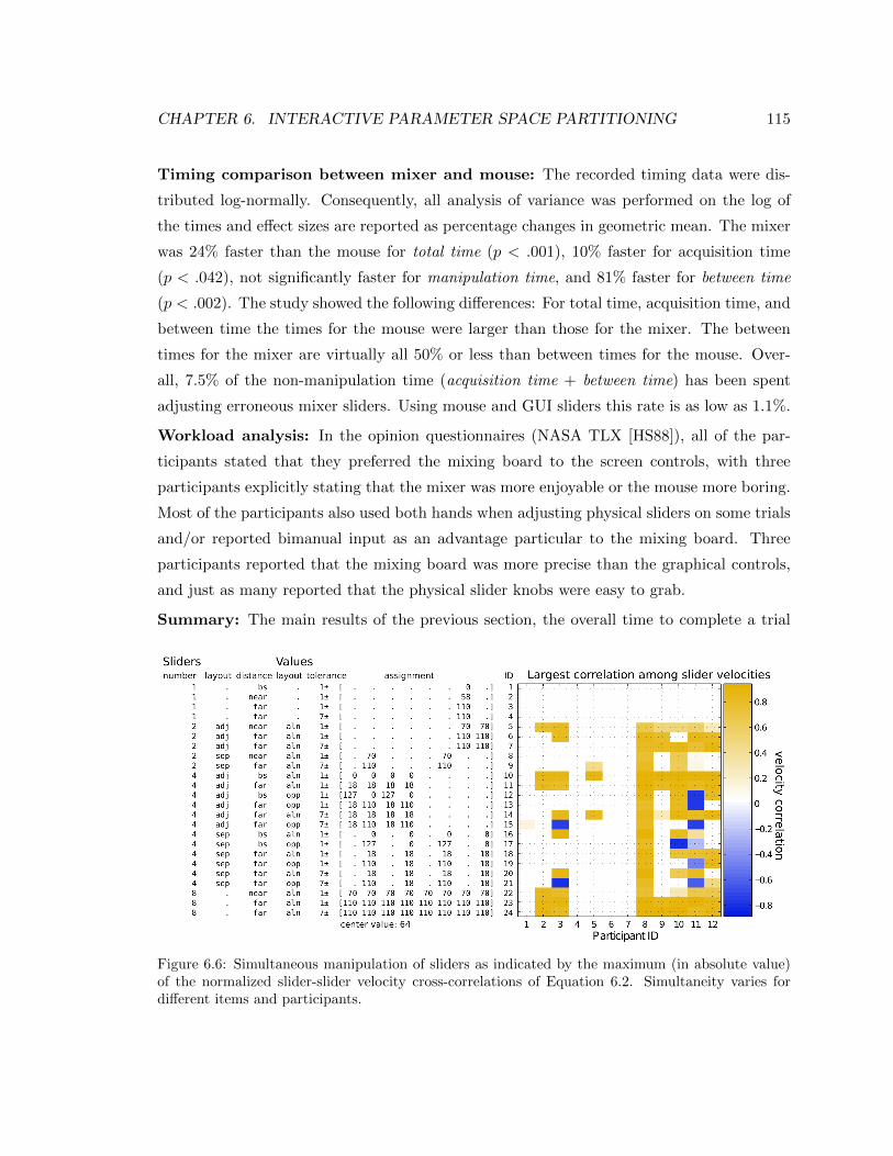
CHAPTER 6. INTERACTIVE PARAMETER SPACE PARTITIONING 115
Timing comparison between mixer and mouse: The recorded timing data were dis-
tributed log-normally. Consequently, all analysis of variance was performed on the log of
the times and effect sizes are reported as percentage changes in geometric mean. The mixer
was 24% faster than the mouse for total time (p < .001), 10% faster for acquisition time
(p < .042), not significantly faster for manipulation time, and 81% faster for between time
(p < .002). The study showed the following differences: For total time, acquisition time, and
between time the times for the mouse were larger than those for the mixer. The between
times for the mixer are virtually all 50% or less than between times for the mouse. Over-
all, 7.5% of the non-manipulation time (acquisition time + between time) has been spent
adjusting erroneous mixer sliders. Using mouse and GUI sliders this rate is as low as 1.1%.
Workload analysis: In the opinion questionnaires (NASA TLX [HS88]), all of the par-
ticipants stated that they preferred the mixing board to the screen controls, with three
participants explicitly stating that the mixer was more enjoyable or the mouse more boring.
Most of the participants also used both hands when adjusting physical sliders on some trials
and/or reported bimanual input as an advantage particular to the mixing board. Three
participants reported that the mixing board was more precise than the graphical controls,
and just as many reported that the physical slider knobs were easy to grab.
Summary: The main results of the previous section, the overall time to complete a trial
Figure 6.6: Simultaneous manipulation of sliders as indicated by the maximum (in absolute value)of the normalized slider-slider velocity cross-correlations of Equation 6.2. Simultaneity varies fordifferent items and participants.

CHAPTER 6. INTERACTIVE PARAMETER SPACE PARTITIONING 116
with mixer interaction is 78% of mouse/GUI pointer based interaction. For items including
extremal values (backstop) the rate can go as low as 72%, corresponding to a gain in speed
of close to 40% when using the mixer.
Determining activity intervals, as described in Section 6.3.2.1, allowed to distinguish the
different periods of non-interaction into initial acquisition time and in-between acquisition
time. The latter is significantly (p < .001) dependent on the input device. Remarkably, the
manipulation time showed no significant dependence.
A trial task was displayed on the screen while the manipulation devices - mixer and
mouse to its right - were placed on the table in front of the screen. Mouse interaction
works via an intermediate pointer or cursor representation on the screen, and thus in the
same visual space the task is presented. The mixing board has its manipulation elements in
physical space. These need to be found using the hands and potentially moving the eye gaze
over to the board. To deal with this situation several participants adopted the strategy of
keeping their gaze on the screen while blindly operating the sliders and occasionally touching
a wrong one. Most of these erroneous manipulations were short term mini-manipulations in
search of the right one to adjust. As reported in the analysis, the overall amount of erroneous
adjustments in the mixer manipulation made only a small difference to the between time
and were higher than the mouse/GUI. Overall, the between time (containing the error time)
was much shorter for the mixer than for the mouse/GUI based interaction.
Applications: The shortened time of interaction and the ability to make simultaneous
adjustments make the mixing board a suitable device for user-guided search over multi-
parameter spaces as it occurs in a variety of application settings. For example, the sliders
could be used to apply ratings of relevance, influencing an algorithm’s notion of good search
results [BSNA+11, TWSM+11, BM10].
Alternatively, parameters may be influenced directly as it would be useful to explore
a design space or to configure visualizations. The user may determine a most promising
direction of exploration by learning about cross-dependencies among different parameters.
With separate adjustments, such as done via the mouse, the direction of the steps in
which one can move through parameter space will always be along parameter axes. With the
simultaneous adjustment of the mixer sliders it is also possible to progress along diagonal
directions in the planes spanned by any pair of parameter axes. This may be helpful for
steering more directly towards optimal configurations.
Another advantage for the mixer in such exploration settings is the fact that it frees up
CHAPTER 6. INTERACTIVE PARAMETER SPACE PARTITIONING 117
screen real estate. With the separate interaction device, the entire display can be used to
show the data in more detail.
In our experiments we have used the motor control of the sliders only to ensure a clearly
defined initial state for each task. However, depending on the application setting there is
more to be gained from this feature. In particular, parameter dependencies and constraints
could be expressed to limit the user’s search of feasible regions, or enable the user to push its
boundaries. In a dynamic query range selection [CBS+07] we have enforced the constraint
that the upper bound slider may always be at a value greater or equal to the lower bound
slider.
Further directions: One could also investigate the integration of a separate slider adjust-
ment as provided by the mixing board with more advanced mouse/GUI interactions [vWvL93,
TS98].
Another comparison could consider touch screen interfaces, such as TouchOSC2, in re-
lation to tactile or haptic ones, like a physical mixing board. The study presented in this
section has inspired follow-up work [STD09] that showed a significantly improved visual
focus on the task display, when physical sliders are used instead of GUI controls, which did
not occur when using touch screen sliders placed in the same prior location of the physical
sliders on a table top display. While they did not obtain the timing improvements docu-
mented in this report, the improved eye gaze focus provides further indication and a possible
explanation of the reduced cognitive load when using the mixer.
The items used in our current study are all fairly structured and contain several identical
values. Further studies could consider more different value combinations, e.g., giving target
points that lie in certain specifically shaped neighbourhoods around the origin. Different
directions of the required steering could be considered, as well as measures of how exhaus-
tively a user explored the feasible options. A readily available binding in the paraglide system
of this chapter could provide the technical setup for such a study.
In summary, the shown characteristics portrayed mixing boards as a good fit for the
purpose of a detailed multi-parameter control. Easy and relatively cheap integration of such
a device into an application is possible. Its strengths should particularly hold in settings
where screen space is precious, and undivided visual focus is crucial.
2http://hexler.net/software/touchosc
CHAPTER 6. INTERACTIVE PARAMETER SPACE PARTITIONING 118
6.4 Validation of paraglide in different use cases
In this section, we discuss qualitative feedback and anecdotal evidence from user interviews
and usage sessions during the later stages of our user-centered design process (see Sec-
tion 6.2). The first stable and iteratively improved versions of paraglide were installed in the
work environment of our three lead users. Overall, paraglide has been in use at several occa-
sions over a period of 4 years, accompanied by weekly meetings of our research focus group
for a period of 2 years, and problem-adaptive meeting frequencies in the domain settings.
We present the summative findings in form of usage examples in which our users (a)
were able to do something that they weren’t able to do without paraglide, (b) could gather
new insights into their model by using paraglide, or (c) felt to be able to conduct some task
more efficient with paraglide than with traditional tools.
6.4.1 Movement patterns of biological aggregations
Semi-automatic screening for interesting solutions: In Section 1.2.1 on page 5 a
conjecture was pointed out that interesting spatial patterns only form with parameter con-
figurations for which the PDE has unstable spatially homogenous steady states. This means
that linear stability analysis can be used to detect the potential for pattern formation.
In the course of this research project, the model developer implemented a function to
compute the type of (in-)stability for a given steady state. She had no problems to make
the feature available in paraglide within few minutes using the compute node interface of
Figure 6.2. Colouring the data points by stability type then helped to focus the pattern
search, because computing the feature based on just the input x takes about 5 seconds,
where a full population density would take 5 minutes per configuration point. With this
computationally cheap screening, it became possible to cover larger areas of the parameter
domain before zoning in on sub-areas to compute more comprehensive output that includes
spatio-temporal patterns.
During one meeting a simple positivity test was implemented this way to answer, within
five minutes, whether any solutions with negative densities were present — providing a very
efficient debugging aid.
Discovering structure: To generate a set of sample points simply by specifying the
containing region, the uniform sampling method, and the requested number of points, was
considered a very convenient way to generate data: “You don’t need to worry about the
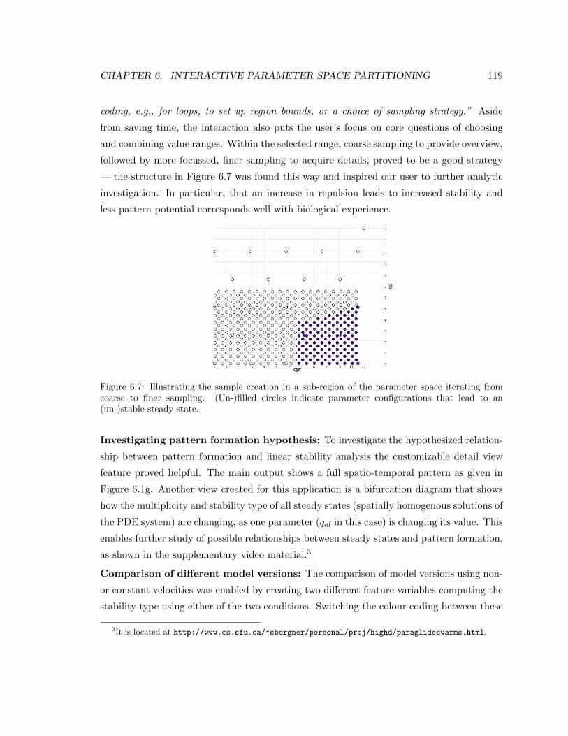
CHAPTER 6. INTERACTIVE PARAMETER SPACE PARTITIONING 119
coding, e.g., for loops, to set up region bounds, or a choice of sampling strategy.” Aside
from saving time, the interaction also puts the user’s focus on core questions of choosing
and combining value ranges. Within the selected range, coarse sampling to provide overview,
followed by more focussed, finer sampling to acquire details, proved to be a good strategy
— the structure in Figure 6.7 was found this way and inspired our user to further analytic
investigation. In particular, that an increase in repulsion leads to increased stability and
less pattern potential corresponds well with biological experience.
Figure 6.7: Illustrating the sample creation in a sub-region of the parameter space iterating fromcoarse to finer sampling. (Un-)filled circles indicate parameter configurations that lead to an(un-)stable steady state.
Investigating pattern formation hypothesis: To investigate the hypothesized relation-
ship between pattern formation and linear stability analysis the customizable detail view
feature proved helpful. The main output shows a full spatio-temporal pattern as given in
Figure 6.1g. Another view created for this application is a bifurcation diagram that shows
how the multiplicity and stability type of all steady states (spatially homogenous solutions of
the PDE system) are changing, as one parameter (qal in this case) is changing its value. This
enables further study of possible relationships between steady states and pattern formation,
as shown in the supplementary video material.3
Comparison of different model versions: The comparison of model versions using non-
or constant velocities was enabled by creating two different feature variables computing the
stability type using either of the two conditions. Switching the colour coding between these
3It is located at http://www.cs.sfu.ca/~sbergner/personal/proj/highd/paraglideswarms.html.
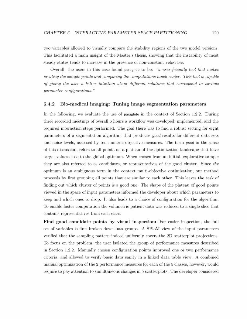
CHAPTER 6. INTERACTIVE PARAMETER SPACE PARTITIONING 120
two variables allowed to visually compare the stability regions of the two model versions.
This facilitated a main insight of the Master’s thesis, showing that the instability of most
steady states tends to increase in the presence of non-constant velocities.
Overall, the users in this case found paraglide to be: “a user-friendly tool that makes
creating the sample points and comparing the computations much easier. This tool is capable
of giving the user a better intuition about different solutions that correspond to various
parameter configurations.”
6.4.2 Bio-medical imaging: Tuning image segmentation parameters
In the following, we evaluate the use of paraglide in the context of Section 1.2.2. During
three recorded meetings of overall 6 hours a workflow was developed, implemented, and the
required interaction steps performed. The goal there was to find a robust setting for eight
parameters of a segmentation algorithm that produces good results for different data sets
and noise levels, assessed by ten numeric objective measures. The term good in the sense
of this discussion, refers to all points on a plateau of the optimization landscape that have
target values close to the global optimum. When chosen from an initial, explorative sample
they are also referred to as candidates, or representatives of the good cluster. Since the
optimum is an ambiguous term in the context multi-objective optimization, our method
proceeds by first grouping all points that are similar to each other. This leaves the task of
finding out which cluster of points is a good one. The shape of the plateau of good points
viewed in the space of input parameters informed the developer about which parameters to
keep and which ones to drop. It also leads to a choice of configuration for the algorithm.
To enable faster computation the volumetric patient data was reduced to a single slice that
contains representatives from each class.
Find good candidate points by visual inspection: For easier inspection, the full
set of variables is first broken down into groups. A SPloM view of the input parameters
verified that the sampling pattern indeed uniformly covers the 2D scatterplot projections.
To focus on the problem, the user isolated the group of performance measures described
in Section 1.2.2. Manually chosen configuration points improved one or two performance
criteria, and allowed to verify basic data sanity in a linked data table view. A combined
manual optimization of the 2 performance measures for each of the 5 classes, however, would
require to pay attention to simultaneous changes in 5 scatterplots. The developer considered
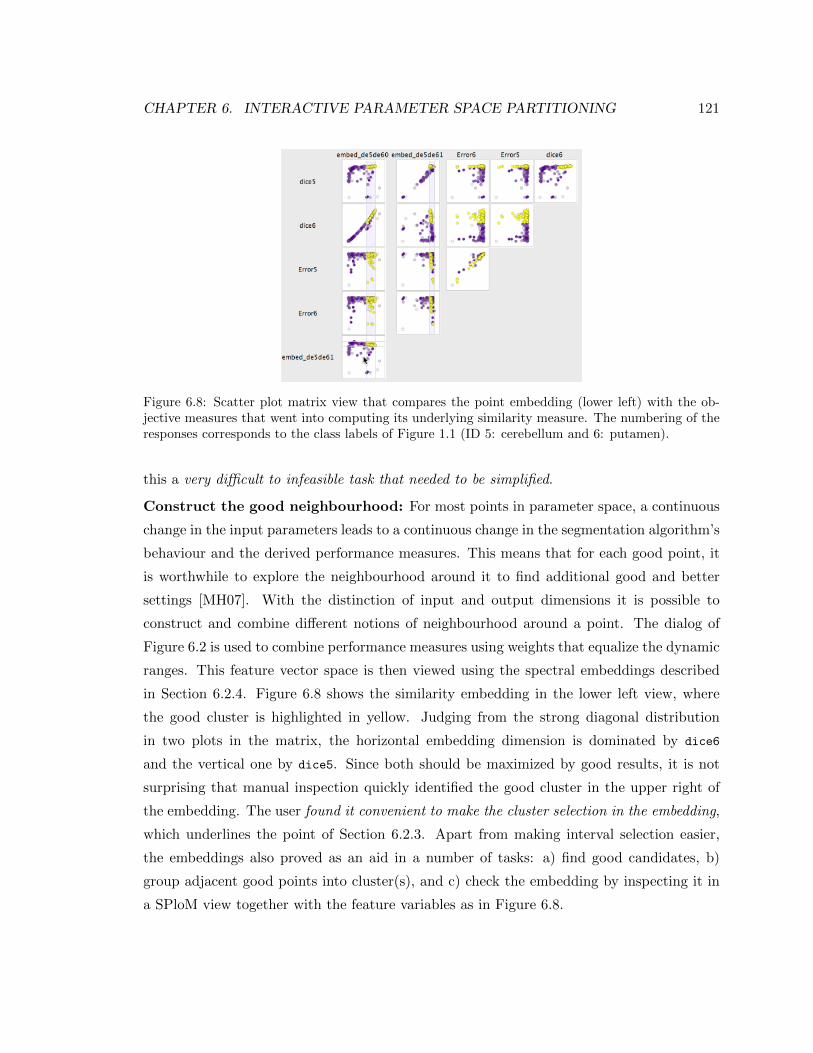
CHAPTER 6. INTERACTIVE PARAMETER SPACE PARTITIONING 121
Figure 6.8: Scatter plot matrix view that compares the point embedding (lower left) with the ob-jective measures that went into computing its underlying similarity measure. The numbering of theresponses corresponds to the class labels of Figure 1.1 (ID 5: cerebellum and 6: putamen).
this a very difficult to infeasible task that needed to be simplified.
Construct the good neighbourhood: For most points in parameter space, a continuous
change in the input parameters leads to a continuous change in the segmentation algorithm’s
behaviour and the derived performance measures. This means that for each good point, it
is worthwhile to explore the neighbourhood around it to find additional good and better
settings [MH07]. With the distinction of input and output dimensions it is possible to
construct and combine different notions of neighbourhood around a point. The dialog of
Figure 6.2 is used to combine performance measures using weights that equalize the dynamic
ranges. This feature vector space is then viewed using the spectral embeddings described
in Section 6.2.4. Figure 6.8 shows the similarity embedding in the lower left view, where
the good cluster is highlighted in yellow. Judging from the strong diagonal distribution
in two plots in the matrix, the horizontal embedding dimension is dominated by dice6
and the vertical one by dice5. Since both should be maximized by good results, it is not
surprising that manual inspection quickly identified the good cluster in the upper right of
the embedding. The user found it convenient to make the cluster selection in the embedding,
which underlines the point of Section 6.2.3. Apart from making interval selection easier,
the embeddings also proved as an aid in a number of tasks: a) find good candidates, b)
group adjacent good points into cluster(s), and c) check the embedding by inspecting it in
a SPloM view together with the feature variables as in Figure 6.8.
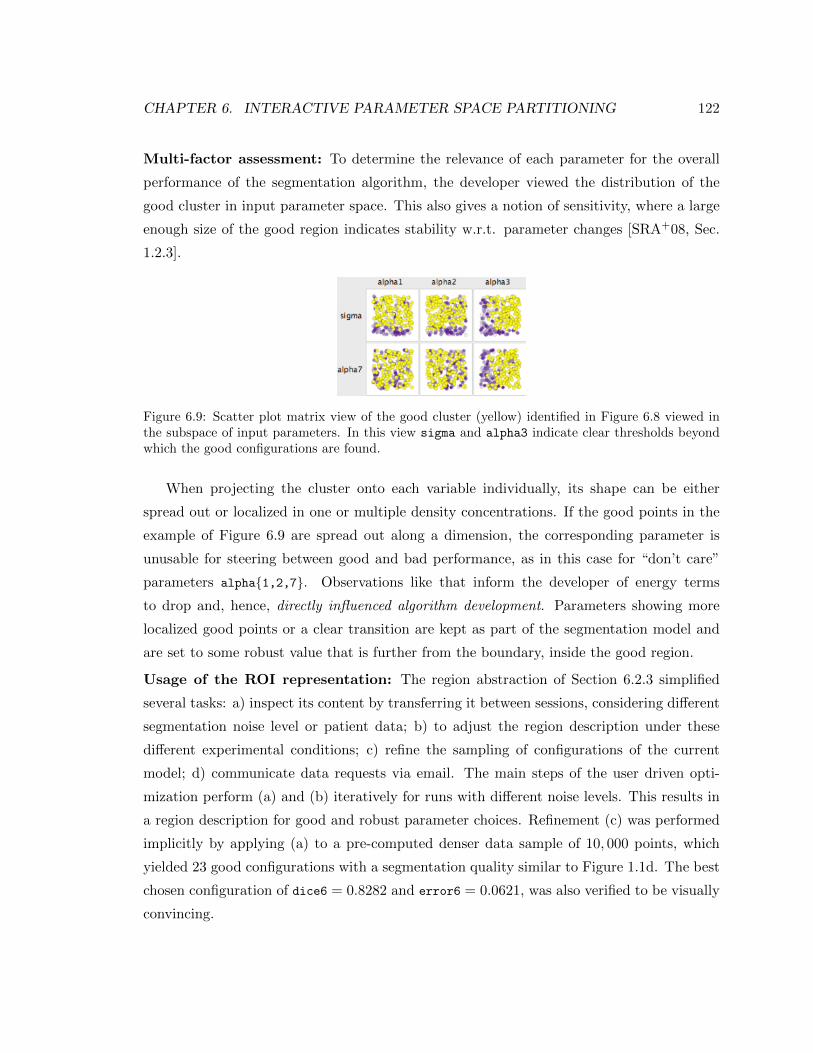
CHAPTER 6. INTERACTIVE PARAMETER SPACE PARTITIONING 122
Multi-factor assessment: To determine the relevance of each parameter for the overall
performance of the segmentation algorithm, the developer viewed the distribution of the
good cluster in input parameter space. This also gives a notion of sensitivity, where a large
enough size of the good region indicates stability w.r.t. parameter changes [SRA+08, Sec.
1.2.3].
Figure 6.9: Scatter plot matrix view of the good cluster (yellow) identified in Figure 6.8 viewed inthe subspace of input parameters. In this view sigma and alpha3 indicate clear thresholds beyondwhich the good configurations are found.
When projecting the cluster onto each variable individually, its shape can be either
spread out or localized in one or multiple density concentrations. If the good points in the
example of Figure 6.9 are spread out along a dimension, the corresponding parameter is
unusable for steering between good and bad performance, as in this case for “don’t care”
parameters alpha1,2,7. Observations like that inform the developer of energy terms
to drop and, hence, directly influenced algorithm development. Parameters showing more
localized good points or a clear transition are kept as part of the segmentation model and
are set to some robust value that is further from the boundary, inside the good region.
Usage of the ROI representation: The region abstraction of Section 6.2.3 simplified
several tasks: a) inspect its content by transferring it between sessions, considering different
segmentation noise level or patient data; b) to adjust the region description under these
different experimental conditions; c) refine the sampling of configurations of the current
model; d) communicate data requests via email. The main steps of the user driven opti-
mization perform (a) and (b) iteratively for runs with different noise levels. This results in
a region description for good and robust parameter choices. Refinement (c) was performed
implicitly by applying (a) to a pre-computed denser data sample of 10, 000 points, which
yielded 23 good configurations with a segmentation quality similar to Figure 1.1d. The best
chosen configuration of dice6 = 0.8282 and error6 = 0.0621, was also verified to be visually
convincing.
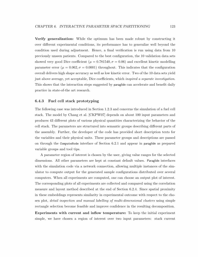
CHAPTER 6. INTERACTIVE PARAMETER SPACE PARTITIONING 123
Verify generalization: While the optimum has been made robust by constructing it
over different experimental conditions, its performance has to generalize well beyond the
condition used during adjustment. Hence, a final verification is run using data from 10
previously unseen patients. Compared to the best configuration, the 10 validation data sets
showed very good Dice coefficient (µ = 0.781540, σ = 0.06) and excellent kinetic modelling
parameter error (µ = 0.062, σ = 0.0001) throughout. This indicates that the configuration
overall delivers high shape accuracy as well as low kinetic error. Two of the 10 data sets yield
just above average, yet acceptable, Dice coefficients, which inspired a separate investigation.
This shows that the interaction steps suggested by paraglide can accelerate and benefit daily
practice in state-of-the art research.
6.4.3 Fuel cell stack prototyping
The following case was introduced in Section 1.2.3 and concerns the simulation of a fuel cell
stack. The model by Chang et al. [CKPW07] depends on about 100 input parameters and
produces 43 different plots of various physical quantities characterizing the behavior of the
cell stack. The parameters are structured into semantic groups describing different parts of
the assembly. Further, the developer of the code has provided short description texts for
the variables and their physical units. These parameter groups and descriptions are passed
on through the ComputeNode interface of Section 6.2.1 and appear in paraglide as prepared
variable groups and tool tips.
A parameter region of interest is chosen by the user, giving value ranges for the selected
dimensions. All other parameters are kept at constant default values. Paraglide interfaces
with the simulation code via a network connection, allowing multiple instances of the sim-
ulator to compute output for the generated sample configurations distributed over several
computers. When all experiments are computed, one can choose an output plot of interest.
The corresponding plots of all experiments are collected and compared using the correlation
measure and layout method described at the end of Section 6.2.4. Since spatial proximity
in these embeddings represents similarity in experimental outcome with respect to the cho-
sen plot, detail inspection and manual labelling of multi-dimensional clusters using simple
rectangle selection become feasible and improve confidence in the resulting decomposition.
Experiments with current and inflow temperature: To keep the initial experiment
simple, we have chosen a region of interest over two input parameters: stack current
CHAPTER 6. INTERACTIVE PARAMETER SPACE PARTITIONING 124
(a) x-stack current, y-in temp.(b) cell current density similar-ity
(c) MEA water content similar-ity
Figure 6.10: Two layouts for 204 example experiments. a) input space showing variation in currentand input temperature, b) embedding of the same samples where spatial proximity reflects plotsimilarity for cell current density, c) similarity embedding for membrane electrode assembly (MEA)water content using the same clusters as assigned in (b). Cluster representatives are shown inFigure 6.11 and Figure 6.12. These screenshots are from the 2007 C++ version of paraglide, and arealso attainable in the currently discussed Java implementation.
(10A..400A) and stack inflow temperature (333K..343K). In this region 204 samples are
created with a uniform random distribution shown in Figure 6.10a. The colour coding is
added at a later stage and has no relevance for the initial step.
In Figure 6.10b the sample configurations are arranged according to their similarity in cell
current density. In this embedding simulation outcomes can be inspected and configuration
sample points can be manually labeled using a screen rectangle selection. For comparison,
another similarity based embedding is shown in Figure 6.10c for the water content of the
membrane-electrode assembly (MEA) using the same cluster labels as Figure 6.10b. When
going back to the input space Figure 6.10a, the colour coding reflects the parameter ranges
of distinct behavior. Cluster representatives are shown in Figure 6.11 and Figure 6.12.
Our users found the parameter space partitioning of Figure 6.10 intriguing, giving them
a new method to study their model. For instance, they pointed out that while cluster
representative Figure 6.11e may be physically unreasonable, the (e) region in Figure 6.10a
can be interpreted as a “bad” region, where adverse reactions occur.
6.5 Discussion and future work
The development of computer simulations needs careful setup of the involved parameters.
The discussed use cases indicated that the required process of understanding can be time

CHAPTER 6. INTERACTIVE PARAMETER SPACE PARTITIONING 125
(a) (b) (c)
(d) (e) (f)
Figure 6.11: Cell current density plots for the clusters in Figure 6.10b
(a) (b) (c)
(d) (e) (f)
Figure 6.12: MEA water content plots for the clusters labelled in Figure 6.10c
CHAPTER 6. INTERACTIVE PARAMETER SPACE PARTITIONING 126
and resource intensive, and that systematic assistance is in order. Our validation of these
investigations showed how the proposed decomposition of the continuous input parameter
space benefits different questions. One finding suggests that even with potentially large
numbers of variables, such a clustering of responses can result in a small number of re-
gions. This can lead to a significant conceptual simplification and narrow down questions
to particular sub-regions. Also, it provides starting points for local sensitivity analyses.
Feasible or interesting regions for large numbers of variables can be relatively small in
volume when compared to their bounding box. This is an example setting, where domain
specific hints can help to guide the choice of sample points. For that, one could seek to
obtain an implicit function representation of the region boundary, that could be used by the
sampling module of Figure 1.3.
ROI usage: In the requirement analysis of Section 1.2 it became apparent that the specifi-
cation of a region of interest (ROI) as discussed in Section 6.2.3 has multiple uses in different
sub-tasks:
• specify a domain or sub-region for sampling to create or refine the data set,
• choose a viewport to focus the overview,
• steer a cursor to set default values or invoke a detail view,
• make a selection of points for subset processing, for instance to manually assign labels,
• filter points to crop the viewed data range in order to deal with occlusion,
• enable mouse manipulation of the region description,
• export/import region descriptions to compare among different data sets.
Basic user interfaces for this purpose have been discussed in Section 6.3.1 and Section 6.3.2.
Exploring these directions further could lead to interesting combinations of user interaction
and dimension reduction. So far, Section 6.2.2.2 presents a very simple, completely manual
approach to this.
Our current implementation (e.g., Section 6.2.2.3) facilitates different point grouping
methods: manual labelling, application of a classifier function, and clustering via a user
determined similarity measure. Since clustering is key to parameter space partitioning,
further research on suitable interactive and (semi-)automatic techniques for this purpose
would be useful.
CHAPTER 6. INTERACTIVE PARAMETER SPACE PARTITIONING 127
Conclusions: The paraglide framework can be seen as a general user interface to work
with simulation code. While software engineering aspects for such a system can not be
disregarded, they should not be seen as the focus of this discussion. The main point of
relevance to visualization research is that all use cases studied here exhibit a common need
for region decomposition of the input parameter space based on a clustering or quantization
of output responses. While fitting and optimization are the usual focus in current literature
(see also the task overview in Section 2.4.1), parameter space partitioning has not yet
received much attention in visualization. By showing its applicability and practical benefits
in settings where a comprehensive understanding of the underlying system is required, we
hope to have stimulated further work in this direction.
Such a decomposition method can use feature extractors, as shown in Section 6.4.1,
employ distance measures in Section 6.4.2 and Section 6.4.3. Both approaches required user
control or at least careful setup to yield informative results. The output is in all cases a
set of continuous, multi-dimensional regions. Envisioning this, our initial research focussed
on high-quality projection techniques for scatter plots of this kind of data. After adjusting
research focus to sampling aspects and the use case evaluation presented here, suitable
options to visually represent a region decomposition of a multi-dimensional continuous space
still deserve further study.
Chapter 7
Discussion and conclusion
In the following I will briefly put the individual discussions of the previous chapters into
perspective. The combining theme of Chapter 1 was emphasizing the importance of involv-
ing human judgement in order to establish correspondence between computational models
and the real-world systems they represent. The conclusion, however, does not follow in all
cases and counter arguments can be made easily. For instance, live sensor measurements
can feed directly into a computational model that adjusts to new conditions as streaming
data arrives. This could happen at a much higher speed and accuracy than a human experi-
menter could copy the sensor readings into a spreadsheet, visually inspect the data for basic
sanity, before crunching the numbers with further algorithmic processing. Nevertheless, at
some early stage of model development and validation it might have been done this way.
In the context of machine learning algorithm development Cohen [CK95, p. 12] states
that the confirmation of a model does not start out as crisp as the final publication typi-
cally presents it. He outlines that the model construction process goes through a number
of phases [CK95, p. 7]: Initial, data-intensive exploratory studies give casual hypotheses,
for which assessment studies provide parameter baselines and ranges. With this informa-
tion, observation and manipulation experiments can then establish statistical evidence for
relevance of certain factors and the effects of different value levels.
Coming from the related field of image analysis, where the objective is also to automate
recognition tasks as much as possible, my entry into data visualization research arose from
the observation that the model development process required good interfaces for scrutiny
and control by the developer. For instance, I had to develop ad-hoc tools to assist the gen-
eration of informative training data [Ber03, §4.2] and the adjustment of higher-level model
128

CHAPTER 7. DISCUSSION AND CONCLUSION 129
parameters (e.g., to find weights for combined ratings or energy terms [Ber03, Eq. 4.13]).
My main point is that many situations are conceivable, where it can be very important
that methods and tools are in place that enable a human to take control over computer mod-
els — development in research, perceptually guided design, and monitoring and response in
unexpected conditions are a few such examples. At the same time, there is a risk that hu-
man interfaces are abused to compensate for insufficient algorithm development, burdening
people with repetitive, demotivating tasks that really should better be done by a computer.
After viewing the argument from both sides, it should have become clear that there is
a line to be drawn that separates algorithmic problems that people should be able to get
involved with, from settings where this involvement should be minimized. At this point, I am
not attempting such a distinction. Rather, do the chapters of this dissertation demonstrate
different roles that a human investigator can take. As outlined in Chapter 1, approaches
range from interactive trial and error adjustments in Chapter 6, to criteria specification that
feeds into an automatic optimization of Chapter 5, to theoretical study of a problem that
enables a systematic parameter choice in Chapter 4, to a uniformly space-filling sampling
method for which the user merely outlines a region of interest and prescribes a budget of
points in Chapter 3.
At the end of Section 2.4, a categorization of different data sources was suggested,
that distinguishes field data (primary), human input (secondary), and theoretically derived
relations or laws (tertiary). The different involvement of secondary and tertiary sources
prescribes the order of the rows in the overview Table 7.1, where, in retrospect, each chapter
is motivated by a general purpose of study. This leads to a decomposition into tasks, which
imply more specific sub-goals or objectives. The role of the user is indicated in each case as
well as the amount of theoretical study that was performed to adress the problem. These
two scales turned out to be somewhat inverse to each other.
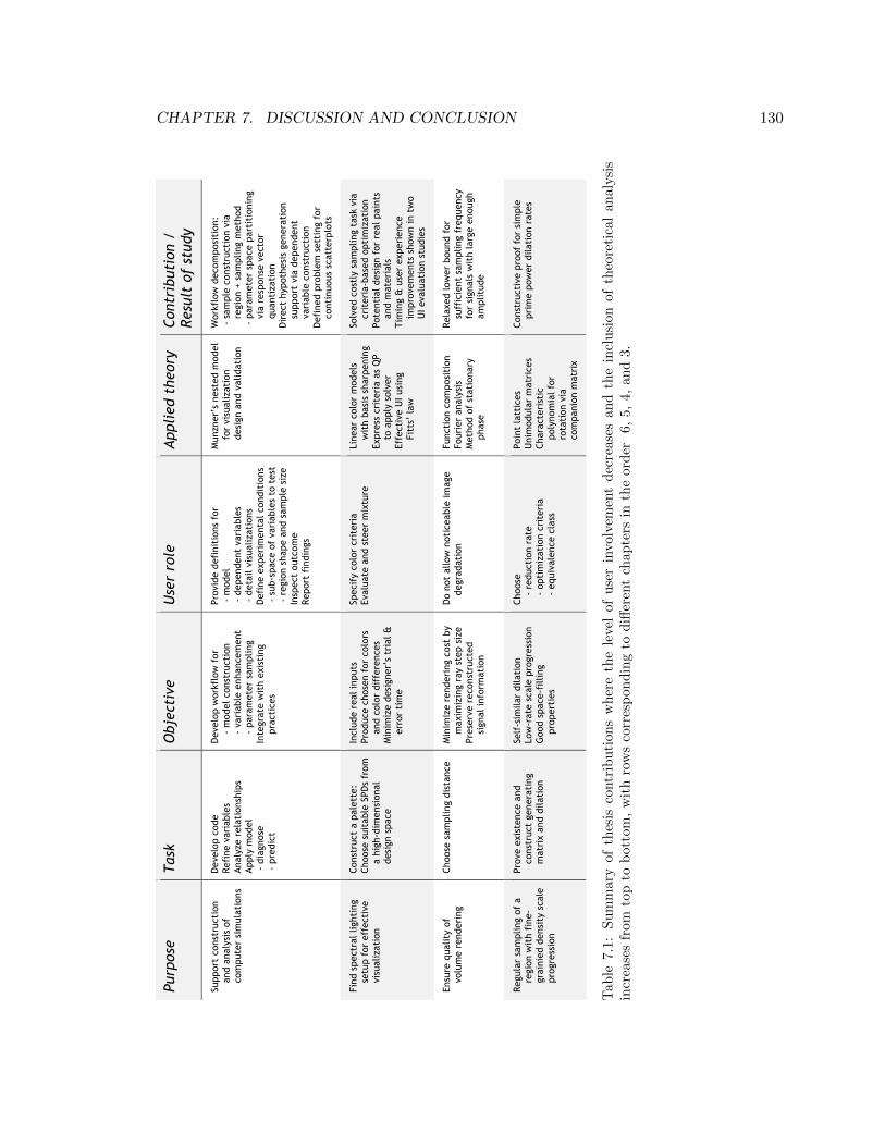
CHAPTER 7. DISCUSSION AND CONCLUSION 130
Purp
ose
Tas
k O
bjec
tive
U
ser
role
A
ppli
ed t
heor
y Con
trib
utio
n /
Res
ult
of s
tudy
Support c
onstructio
n
and a
naly
sis
of
com
puter s
imula
tio
ns
Develo
p c
ode
Refi
ne v
aria
ble
s
Analy
ze r
ela
tio
nship
s
Apply
model
- d
iagnose
- p
redic
t
Develo
p w
orkfl
ow
for
- m
odel
constructio
n
- varia
ble
enhancem
ent
- param
eter s
am
pling
Integrate w
ith e
xis
tin
g
practic
es
Provid
e d
efi
nit
ions f
or
- m
odel
- d
ependent v
aria
ble
s
- d
etail v
isualizatio
ns
Defi
ne e
xperim
ental condit
ions
- s
ub-s
pace o
f varia
ble
s t
o t
est
- r
egio
n s
hape a
nd s
am
ple
siz
e
Inspect o
utcom
e
Report f
indin
gs
Munzner’s
nested m
odel
for v
isualizatio
n
desig
n a
nd v
alidatio
n
Workfl
ow
decom
posit
ion:
- s
am
ple
constructio
n v
ia
regio
n +
sam
pling m
ethod
- p
aram
eter s
pace p
artit
ionin
g
via
response v
ector
quantiz
atio
n
Dir
ect h
ypothesis
generatio
n
support v
ia d
ependent
varia
ble
constructio
n
Defi
ned p
roble
m s
ettin
g f
or
contin
uous s
catterplo
ts
Fin
d s
pectral lightin
g
setup f
or e
ffectiv
e
vis
ualizatio
n
Construct a
pale
tte:
Choose s
uit
able
SPD
s f
rom
a h
igh-d
imensio
nal
desig
n s
pace
Inclu
de r
eal
inputs
Produce c
hosen f
or c
olo
rs
and c
olo
r d
iffe
rences
Min
imiz
e d
esig
ner’s
tria
l &
error t
ime
Specif
y c
olo
r c
rit
eria
Evalu
ate a
nd s
teer m
ixture
Lin
ear c
olo
r m
odels
wit
h b
asis
sharpenin
g
Express c
rit
eria
as Q
P
to a
pply
solv
er
Eff
ectiv
e U
I usin
g
Fit
ts’
law
Solv
ed c
ostly
sam
pling t
ask v
ia
crit
eria
-based o
ptim
izatio
n
Potentia
l desig
n f
or r
eal pain
ts
and m
ateria
ls
Tim
ing &
user e
xperie
nce
improvem
ents s
how
n in t
wo
UI evalu
atio
n s
tudie
s
Ensure q
uality o
f
volu
me r
enderin
g
Choose s
am
pling d
istance
Min
imiz
e r
enderin
g c
ost b
y
maxim
izin
g r
ay s
tep s
ize
Preserve r
econstructed
sig
nal in
form
atio
n
Do n
ot a
llow
notic
eable
im
age
degradatio
n
Functio
n c
om
posit
ion
Fourie
r a
naly
sis
Method o
f statio
nary
phase
Rela
xed low
er b
ound f
or
suff
icie
nt s
am
pling f
requency
for s
ignals
wit
h large e
nough
am
plitude
Regula
r s
am
pling o
f a
regio
n w
ith f
ine-
grain
ied d
ensit
y s
cale
progressio
n
Prove e
xis
tence a
nd
construct g
eneratin
g
matrix
and d
ilatio
n
Self
-sim
ilar d
ilatio
n
Low
-rate s
cale
progressio
n
Good s
pace-f
illing
propertie
s
Choose
- reductio
n r
ate
- optim
izatio
n c
rit
eria
- equiv
ale
nce c
lass
Poin
t l
attic
es
Unim
odula
r m
atric
es
Characteris
tic
poly
nom
ial fo
r
rotatio
n v
ia
com
panio
n m
atrix
Constructiv
e p
roof
for s
imple
prim
e p
ow
er d
ilatio
n r
ates
Tab
le7.
1:S
um
mar
yof
thes
isco
ntr
ibu
tion
sw
her
eth
ele
vel
of
use
rin
volv
emen
td
ecre
ase
san
dth
ein
clu
sion
of
theo
reti
cal
an
aly
sis
incr
ease
sfr
omto
pto
bot
tom
,w
ith
row
sco
rres
pon
din
gto
diff
eren
tch
ap
ters
inth
eord
er6,
5,
4,
an
d3.
CHAPTER 7. DISCUSSION AND CONCLUSION 131
7.1 Conclusion
Beginning the exposition of my dissertation by characterizing practical domains of study
that employ computational models in settings that required involvement of human judge-
ment, which included a model of biological aggregations, image segmentation methods, and
rendering algorithms — I derived a set of requirements to propose a framework for user-
driven analysis of parameter effects. A novel outcome of the workflow I suggested was a
partitioning of the continuous space of model configurations into regions of distinct system
behaviour.
To facilitate progressive regional exploration, I devised a space-filling sampling method
by constructing point lattices that contain rotated and scaled versions of themselves. All
resolution levels of this construction share a single type of Voronoi polytope, whose volume
grows independently of the dimensionality by a chosen integer factor as low as 2.
With the goal of reducing sampling costs while maintaining image quality when rendering
volumetric data, I performed a Fourier domain analysis of the effect of composing two
functions. Based on this, I relaxed a previous lower bound for a sufficient sampling frequency
and applied it to adaptively choose the step size in raycasting.
After suggesting that spectral light models in computer graphics can not only be used
to improve physical realism, but also to create colour effects that scale the level of distin-
guishable detail in a visualization, I developed a method that helps designers to choose a
setup from a high-dimensional parameter space of possible palettes of spectral power dis-
tributions, to optimally fulfill a number of user-specified criteria. Given such a palette of
materials and lights, a remaining task is to choose a desired mixture of presets, for which I
studied two alternative interaction methods and showed how each of them either improves
timing performance or reduces cognitive load, both aspects bear the potential to improve
the quality of the outcome of the task.
Despite the apparent diversity, the selection of research that is combined in this disser-
tation partitions a common space of approaches to human-driven improvement of computa-
tional models through the lens of parameter adjustments. Hopefully, this contributes to a
more comprehensive understanding. Related topics, beyond the scope of this thesis, could
study direct interfaces between computational models or — on the other side — seek to
improve interaction among people.
Appendix A
Mathematical concepts related to data
analysis
A relation is a set of I-tuples xii∈I with index set I, where n-ary relations consist of n-
tuples with index set I = 1 . . . n. A function f : X → Y corresponds to a binary relation
R of domain X and range Y such that for x ∈ X and y, z ∈ Y xRy and xRz implies y = z,
i.e. every element in the domain is mapped to only one element of the range. To define a
notion of continuity for such a mapping, we will first consider some topological concepts.
A.1 Topology and geometry
A topology τ on a set X is a collection of subsets of X satisfying: 1. ∅, X ∈ τ , 2. τ is closed
under finite intersections, 3. τ is closed under arbitrary unions. A non-empty set equipped
with topology τ is referred to as topological space (X, τ). An element of τ is also called
neighbourhood or open set in X. The complement of an open set is a closed set. The trivial
topology consists of only ∅ and X. The discrete topology consists of all subsets of X.
A function f : X → Y between topological spaces is continuous if f−1(U) is open in
X for each open set U in Y . One says that f is continuous at the point x, if f−1(V ) is a
neighbourhood of x whenever V is a neighbourhood of f(x) [AB06, p. 36]. An equivalent
definition in metric spaces is given in the next section.
A homeomorphism is a one-to-one correspondence that is continuous in both directions.
Properties of point sets that are not affected by such transformations are called topological
invariants with examples given in Section 2.1.
132
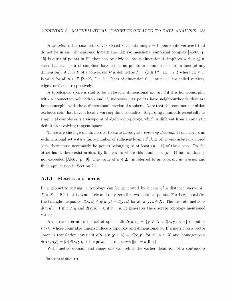
APPENDIX A. MATHEMATICAL CONCEPTS RELATED TO DATA ANALYSIS 133
A simplex is the smallest convex closed set containing r + 1 points (its vertices) that
do not lie in an r dimensional hyperplane. An r-dimensional simplicial complex [Ale65, p.
15] is a set of points in Rn that can be divided into r-dimensional simplices with r ≤ n,
such that each pair of simplices have either no points in common or share a face (of any
dimension). A face F of a convex set P is defined as F = x ∈ Rn : cx = c0 where cx ≤ c0
is valid for all x ∈ P [Zie95, Ch. 2]. Faces of dimension 0, 1, or n − 1 are called vertices,
edges, or facets, respectively.
A topological space is said to be a closed n-dimensional manifold if it is homeomorphic
with a connected polyhedron and if, moreover, its points have neighbourhoods that are
homeomorphic with the n-dimensional interior of a sphere. Note that this common definition
excludes sets that have a locally varying dimensionality. Regarding manifolds essentially as
simplicial complexes is a viewpoint of algebraic topology, which is different from an analytic
definition involving tangent spaces.
These are the ingredients needed to state Lebesgue’s covering theorem: If one covers an
n-dimensional set with a finite number of sufficiently small1, but otherwise arbitrary closed
sets, there must necessarily be points belonging to at least (n + 1) of these sets. On the
other hand, there exist arbitrarily fine covers where this number of (n + 1) intersections is
not exceeded [Ale65, p. 9]. The value of n ∈ Z+ is referred to as covering dimension and
finds application in Section 2.1.
A.1.1 Metrics and norms
In a geometric setting, a topology can be generated by means of a distance metric d :
X ×X → R+ that is symmetric and only zero for two identical points. Further, it satisfies
the triangle inequality d(x, z) ≤ d(x,y) + d(y, z) for all x,y, z ∈ X. The discrete metric is
d(x, y) = 1 if x 6= y and d(x, y) = 0 if x = y. It generates the discrete topology mentioned
earlier.
A metric determines the set of open balls B(x, r) = y ∈ X : d(x,y) < r of radius
r > 0, whose countable unions induce a topology and dimensionality. If a metric on a vector
space is translation invariant d(x + a,y + a) = d(x,y) for all a ∈ X and homogeneous
d(αx, αy) = |α| d(x,y), it is equivalent to a norm ‖x‖ = d(0,x).
With metric domain and range one can refine the earlier definition of a continuous
1in terms of diameter
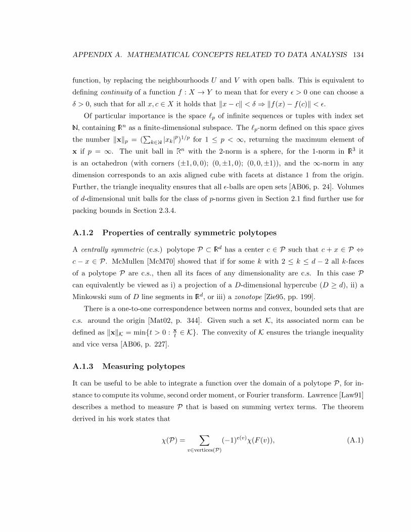
APPENDIX A. MATHEMATICAL CONCEPTS RELATED TO DATA ANALYSIS 134
function, by replacing the neighbourhoods U and V with open balls. This is equivalent to
defining continuity of a function f : X → Y to mean that for every ε > 0 one can choose a
δ > 0, such that for all x, c ∈ X it holds that ‖x− c‖ < δ ⇒ ‖f(x)− f(c)‖ < ε.
Of particular importance is the space `p of infinite sequences or tuples with index set
N, containing Rn as a finite-dimensional subspace. The `p-norm defined on this space gives
the number ‖x‖p = (∑
k∈N |xk|p)1/p for 1 ≤ p < ∞, returning the maximum element of
x if p = ∞. The unit ball in Rn with the 2-norm is a sphere, for the 1-norm in R3 it
is an octahedron (with corners (±1, 0, 0); (0,±1, 0); (0, 0,±1)), and the ∞-norm in any
dimension corresponds to an axis aligned cube with facets at distance 1 from the origin.
Further, the triangle inequality ensures that all ε-balls are open sets [AB06, p. 24]. Volumes
of d-dimensional unit balls for the class of p-norms given in Section 2.1 find further use for
packing bounds in Section 2.3.4.
A.1.2 Properties of centrally symmetric polytopes
A centrally symmetric (c.s.) polytope P ⊂ Rd has a center c ∈ P such that c + x ∈ P ⇔c − x ∈ P. McMullen [McM70] showed that if for some k with 2 ≤ k ≤ d − 2 all k-faces
of a polytope P are c.s., then all its faces of any dimensionality are c.s. In this case Pcan equivalently be viewed as i) a projection of a D-dimensional hypercube (D ≥ d), ii) a
Minkowski sum of D line segments in Rd, or iii) a zonotope [Zie95, pp. 199].
There is a one-to-one correspondence between norms and convex, bounded sets that are
c.s. around the origin [Mat02, p. 344]. Given such a set K, its associated norm can be
defined as ‖x‖K = mint > 0 : xt ∈ K. The convexity of K ensures the triangle inequality
and vice versa [AB06, p. 227].
A.1.3 Measuring polytopes
It can be useful to be able to integrate a function over the domain of a polytope P, for in-
stance to compute its volume, second order moment, or Fourier transform. Lawrence [Law91]
describes a method to measure P that is based on summing vertex terms. The theorem
derived in his work states that
χ(P) =∑
v∈vertices(P)
(−1)e(v)χ(F (v)), (A.1)
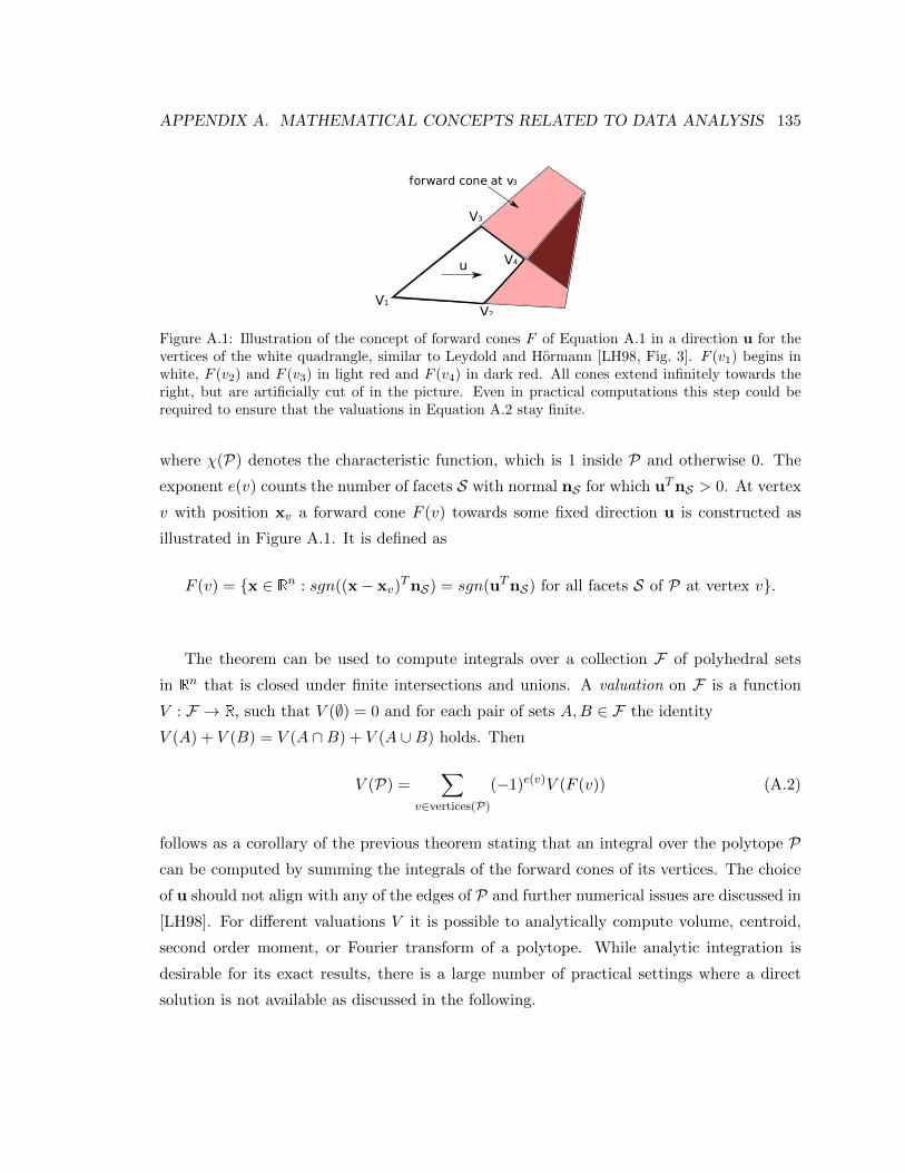
APPENDIX A. MATHEMATICAL CONCEPTS RELATED TO DATA ANALYSIS 135
V3
V1
V2
V4
forward cone at v3
u
Figure A.1: Illustration of the concept of forward cones F of Equation A.1 in a direction u for thevertices of the white quadrangle, similar to Leydold and Hormann [LH98, Fig. 3]. F (v1) begins inwhite, F (v2) and F (v3) in light red and F (v4) in dark red. All cones extend infinitely towards theright, but are artificially cut of in the picture. Even in practical computations this step could berequired to ensure that the valuations in Equation A.2 stay finite.
where χ(P) denotes the characteristic function, which is 1 inside P and otherwise 0. The
exponent e(v) counts the number of facets S with normal nS for which uTnS > 0. At vertex
v with position xv a forward cone F (v) towards some fixed direction u is constructed as
illustrated in Figure A.1. It is defined as
F (v) = x ∈ Rn : sgn((x− xv)TnS) = sgn(uTnS) for all facets S of P at vertex v.
The theorem can be used to compute integrals over a collection F of polyhedral sets
in Rn that is closed under finite intersections and unions. A valuation on F is a function
V : F → R, such that V (∅) = 0 and for each pair of sets A,B ∈ F the identity
V (A) + V (B) = V (A ∩B) + V (A ∪B) holds. Then
V (P) =∑
v∈vertices(P)
(−1)e(v)V (F (v)) (A.2)
follows as a corollary of the previous theorem stating that an integral over the polytope Pcan be computed by summing the integrals of the forward cones of its vertices. The choice
of u should not align with any of the edges of P and further numerical issues are discussed in
[LH98]. For different valuations V it is possible to analytically compute volume, centroid,
second order moment, or Fourier transform of a polytope. While analytic integration is
desirable for its exact results, there is a large number of practical settings where a direct
solution is not available as discussed in the following.
APPENDIX A. MATHEMATICAL CONCEPTS RELATED TO DATA ANALYSIS 136
A.1.4 How the Euclidean norm induces Euclidean topology
The open ε-balls B(p, ε) for all x ∈ X are a basis forming the topology induced by the
underlying norm. Two norms are equivalent if there are two positive constants c1, c2 such
that c1‖x‖a ≤ ‖x‖b ≤ c2‖x‖a for all x ∈ X. Equivalent norms induce the same topology.
A Cartesian product of sets X1 × X2 × ... × Xn is the set of n-tuples (x1, x2, ..., xn),
with xi ∈ Xi. Euclidean space Rn is the Cartesian product of n sets of real numbers.
The topology of the real numbers can be generated from unions and finite intersections of
open intervals (a, b). The multi-dimensional Euclidean topology can be generated from open
boxes (without their boundary) made of open intervals (ai, bi) along each of the n coordinate
axes. To construct a box as intersection of n open sets Ri−1 × (ai, bi) × Rn−i shows how
generators of the topology of the real line extend to generators of Euclidean topology of Rn.
To see the equivalence to the topology induced by a norm, note that these open boxes
coincide with the ε-balls of the ‖·‖∞ norm. For finite dimensional spaces the ‖·‖p norms
are equivalent for p = 1, ...,∞. This shows how the Euclidean 2-norm and, equivalently, all
p-norms on Rn induce Euclidean topology.2
A.2 Function spaces
Function reconstruction with linear models, as will be discussed in Section B.2 on page 145,
is carried out in a vector space F(Rn) of continuous functions over the multi-dimensional
real domain. This space is equipped with an inner product
〈·, ·〉 : F × F → C with the following properties:
1. 〈f, f〉 is real and positive for all f 6= 0 and 〈0, 0〉 = 0,
2. 〈f, g〉 = 〈g, f〉∗ for all f, g ∈ F , where ∗ denotes complex conjugation,
3. 〈αf, g〉 = α〈f, g〉 for any scalar α and f, g ∈ F ,
4. 〈f, g + h〉 = 〈f, g〉+ 〈f, h〉 for all f, g, h ∈ F .
Two vectors or functions are considered to be orthogonal, if their inner product is zero. The
product induces a norm ‖f‖2 =√〈f, f〉, under which all Cauchy sequences converge to an
element in F , which makes the space complete [Gri02, p. 107].
2The description in this section follows a discussion with Ramsay Dyer.
APPENDIX A. MATHEMATICAL CONCEPTS RELATED TO DATA ANALYSIS 137
A space F that has an inner product and a countable basis is referred to as Hilbert
space. An application of this theory in the context of function reconstruction is discussed
in Appendix B.2.3.
In F one can define an orthonormal set ϕl ⊂ F by the condition 〈ϕl, ϕk〉 = δ(k− l) for
any l, k ∈ Z and δ(k) = 0 for k 6= 0 and δ(0) = 1. It fulfills Bessel’s inequality∑∞
l=0 |cl|2 ≤
‖f‖2 with cl = 〈ϕl, f〉 for any f ∈ F . This inequality turns into Parseval’s equality, if and
only if ϕl is a basis, giving a unique vector (cl) ∈ `2 (defined in Section A.1.1 for any
f ∈ F [Gri02, p. 191].
Lebesgue spaces, commonly denoted as Lp(Rn) spaces, are defined to contain all functions
of finite norm
f ∈ Lp ⇔ ‖f‖p =
(∫Rn
|f(x)|p dnx)1/p
<∞. (A.3)
The space L2 of square integrable functions has the inner product
〈f, g〉 =
∫Rn
f∗(x)g(x)dnx (A.4)
and contains all f , for which the induced norm ‖f‖2 is finite. One should note that under this
norm each function is equivalent to a number of functions that agree to it almost everywhere.
In particular, two functions of zero distance ‖g−f‖2 = 0 can disagree g(x) 6= f(x) at points
x ∈ X ⊂ R as long as volnX = 0, e.g., X is any countable set of points.
The dimensionality of a function space is the cardinality of a basis for the space or the
number of independent parameters needed to identify an element in the space. To give an
example, each element of∏n−1, the space of polynomials of degree up to n−1, is determined
by n coefficients.
In machine learning settings, one encounters resolution (time steps, pixels) as a mea-
sure of dimension. For instance, it is common to consider a 1000 × 1000 pixel gray-scale
image as a 106-dimensional vector, where each pixel is one basis function. This number
changes depending on the resolution of the image. A method to determine the true intrinsic
dimensionality as discussed in Section 2.1 can help to guide the choice in this case. An-
other approach is given by the band-limit or number of non-zero coefficients in the Fourier
expansion of a function given in Equation B.6, which also implies a dimensionality for the
function space.

APPENDIX A. MATHEMATICAL CONCEPTS RELATED TO DATA ANALYSIS 138
Mulero-Martınez [MM07] discusses trade-offs between smoothness and dimensionality
of a function space for an approximation via Gaussian RBFs using neural networks. He
builds on an analysis by Sanner and Slotine [SS92], who consider a representation of multi-
dimensional band-limited functions using Gaussian basis functions centred on a regular
lattice.Through slight oversampling, the class of interpolating functions is extended, allowing
for non-canonical reconstruction kernels when accepting vanishingly small approximation
errors. See Section B.2.3 for further analysis of the order of this approximation scheme.
Appendix B
Background on multi-dimensional
sampling
The background provided in this section is relevant to the topic of discretizing computational
function descriptions and supplementary to Chapter 2.
B.1 Uniformity criteria for integration
In continuation of the discussion of quadrature of Section 2.2 on page 23 this section deals
with sampling criteria as they arise in the context of numerical integration with wide ranging
applications that include solutions to equations governing the transport of light [PH04a, pp.
721] and money [SW98, HSW04].
B.1.1 A measure of uniformity
The goal for Quasi-Monte-Carlo methods is to construct deterministic point sets that lead
to favourable error bounds when used in quadrature rules. A common measure of uniformity
is discrepancy ([PH04a, p. 317]; [Nie92, p. 14]), which is defined as
D(X,A) =
∣∣∣∣∣voln(A)− 1
m
m∑i=1
χA(xk)
∣∣∣∣∣ (B.1)
D(X,A) = supA∈A
D(X,A). (B.2)
139
APPENDIX B. BACKGROUND ON MULTI-DIMENSIONAL SAMPLING 140
The supremum picks out the worst case error among all sets A ∈ A, when approximating
a volume, given by the n-dimensional Lebesgue measure voln, by counting points of X that
fall into the support of an indicator function χA. Notice the technical detail that some
authors omit the normalization by the number of sample points in D(X,A) resulting in a
definition that is increased by the factor m.
The standard choice for the set family are corners C or, more precisely, axis aligned boxes
within the unit cube [0, 1]n with one corner anchored at the origin. For this case, one speaks
of the star-discrepancy D∗. Indicator functions for non-anchored boxes can be assembled
via a weighted sum of 2n anchored boxes and so can a bound of their discrepancy [Nie92,
p. 15].
Instead of using the supremum in Equation B.2 it is also possible to compute an average
of D(A,X)p over all sets A ∈ A giving the so-called Lp discrepancy. However, especially
in a higher-dimensional setting the average volume of a box is very small and, thus, the L2
discrepancy is not a good measure of uniformity, as pointed out by Matousek [Mat99, pp.
13], who also provides a discussion of discrepancy for other set systems, such as spheres and
half-planes.
A variation on this theme are digital nets that yield zero discrepancy for the class of
axis aligned boxes that have edge lengths of b−k for some low b ∈ 2, 3, 4, . . . and k =
0 . . . dlnbme that at each scale level k are translated to tile the unit cube at scale k = 0.
Efficient construction methods for such point sets have been devised by Sobol, Niederreiter,
and Keller to name a few ([Nie92, Ch. 4], [Mat99, pp. 51], [KK02]).
Numerical experiments: To give an intuition for why the Cartesian lattice Zn is a
particularly bad choice for quadrature rules, the illustration in Figure B.1a shows how the
number of points in the unit cube changes when scaling the lattice Zn, which is equivalent to
plotting the discrepancy of Equation B.1 for differently scaled cubes anchored at the origin
as required for D(X, C) of Equation B.2. Worst-case discrepancy occurs at the discontinuous
deviations from the exact volume estimate given by the cyan diagonal line. These jumps
arise from sheets of points that simultaneously enter the axis aligned cube. As their count
grows exponentially with increasing dimensionality n, so does the discrepancy of this lattice.
A simple fix to this situation is possible by applying a random rotation to the Cartesian
lattice, since it disturbs this disadvantageous alignment with the coordinate axes. In 3D,
Figure B.1b shows the resulting improvement in discrepancy between the black and the cyan
curve, representing discrepancy for an aligned and rotated sampling lattice, respectively.
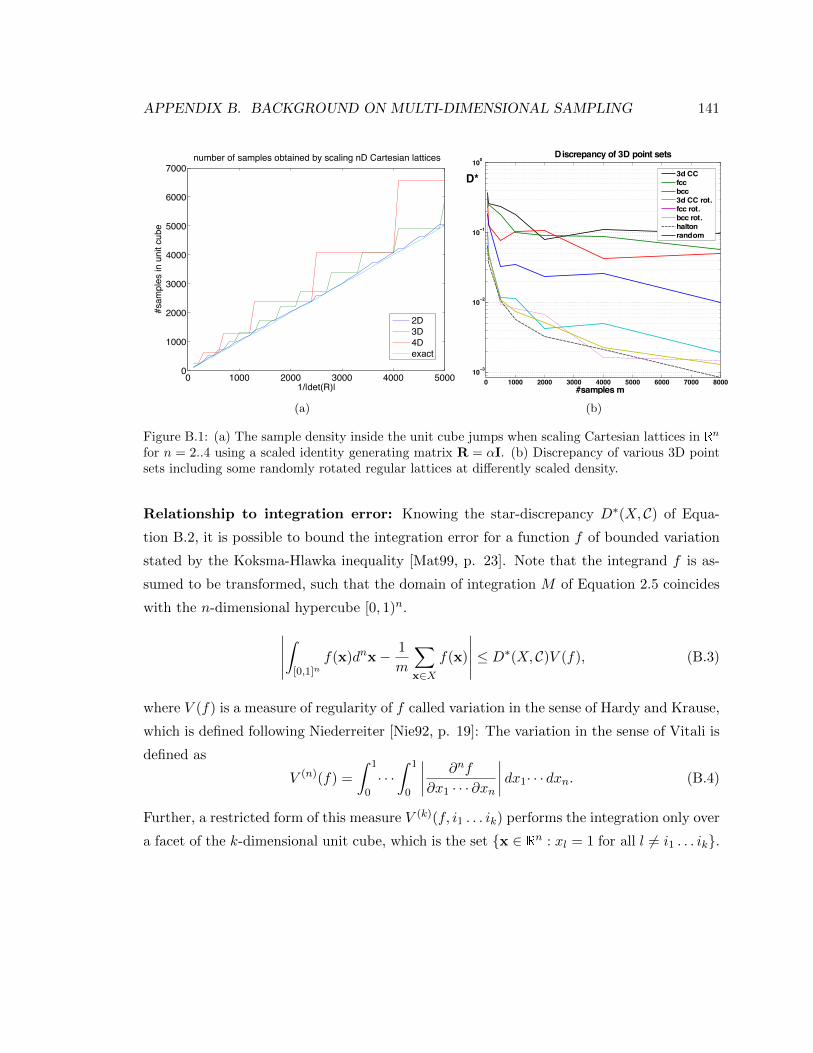
APPENDIX B. BACKGROUND ON MULTI-DIMENSIONAL SAMPLING 141
0 1000 2000 3000 4000 50000
1000
2000
3000
4000
5000
6000
7000
1/|det(R)|
#sam
ples
in u
nit c
ube
number of samples obtained by scaling nD Cartesian lattices
2D3D4Dexact
(a)
(b)
Figure B.1: (a) The sample density inside the unit cube jumps when scaling Cartesian lattices in Rn
for n = 2..4 using a scaled identity generating matrix R = αI. (b) Discrepancy of various 3D pointsets including some randomly rotated regular lattices at differently scaled density.
Relationship to integration error: Knowing the star-discrepancy D∗(X, C) of Equa-
tion B.2, it is possible to bound the integration error for a function f of bounded variation
stated by the Koksma-Hlawka inequality [Mat99, p. 23]. Note that the integrand f is as-
sumed to be transformed, such that the domain of integration M of Equation 2.5 coincides
with the n-dimensional hypercube [0, 1)n.∣∣∣∣∣∫
[0,1]nf(x)dnx− 1
m
∑x∈X
f(x)
∣∣∣∣∣ ≤ D∗(X, C)V (f), (B.3)
where V (f) is a measure of regularity of f called variation in the sense of Hardy and Krause,
which is defined following Niederreiter [Nie92, p. 19]: The variation in the sense of Vitali is
defined as
V (n)(f) =
∫ 1
0· · ·∫ 1
0
∣∣∣∣ ∂nf
∂x1 · · · ∂xn
∣∣∣∣ dx1· · · dxn. (B.4)
Further, a restricted form of this measure V (k)(f, i1 . . . ik) performs the integration only over
a facet of the k-dimensional unit cube, which is the set x ∈ Rn : xl = 1 for all l 6= i1 . . . ik.
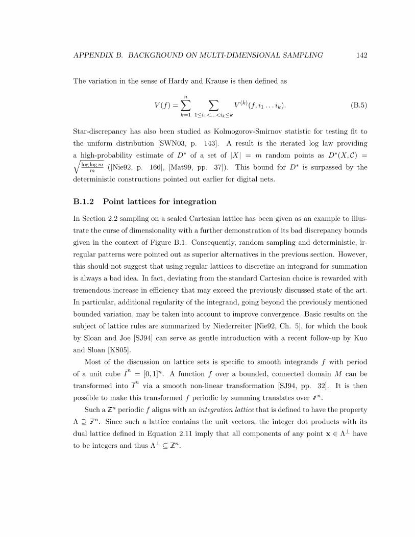
APPENDIX B. BACKGROUND ON MULTI-DIMENSIONAL SAMPLING 142
The variation in the sense of Hardy and Krause is then defined as
V (f) =n∑k=1
∑1≤i1<...<ik≤k
V (k)(f, i1 . . . ik). (B.5)
Star-discrepancy has also been studied as Kolmogorov-Smirnov statistic for testing fit to
the uniform distribution [SWN03, p. 143]. A result is the iterated log law providing
a high-probability estimate of D∗ of a set of |X| = m random points as D∗(X, C) =√log logm
m ([Nie92, p. 166], [Mat99, pp. 37]). This bound for D∗ is surpassed by the
deterministic constructions pointed out earlier for digital nets.
B.1.2 Point lattices for integration
In Section 2.2 sampling on a scaled Cartesian lattice has been given as an example to illus-
trate the curse of dimensionality with a further demonstration of its bad discrepancy bounds
given in the context of Figure B.1. Consequently, random sampling and deterministic, ir-
regular patterns were pointed out as superior alternatives in the previous section. However,
this should not suggest that using regular lattices to discretize an integrand for summation
is always a bad idea. In fact, deviating from the standard Cartesian choice is rewarded with
tremendous increase in efficiency that may exceed the previously discussed state of the art.
In particular, additional regularity of the integrand, going beyond the previously mentioned
bounded variation, may be taken into account to improve convergence. Basic results on the
subject of lattice rules are summarized by Niederreiter [Nie92, Ch. 5], for which the book
by Sloan and Joe [SJ94] can serve as gentle introduction with a recent follow-up by Kuo
and Sloan [KS05].
Most of the discussion on lattice sets is specific to smooth integrands f with period
of a unit cube In
= [0, 1]n. A function f over a bounded, connected domain M can be
transformed into In
via a smooth non-linear transformation [SJ94, pp. 32]. It is then
possible to make this transformed f periodic by summing translates over Zn.
Such a Zn periodic f aligns with an integration lattice that is defined to have the property
Λ ⊇ Zn. Since such a lattice contains the unit vectors, the integer dot products with its
dual lattice defined in Equation 2.11 imply that all components of any point x ∈ Λ⊥ have
to be integers and thus Λ⊥ ⊆ Zn.
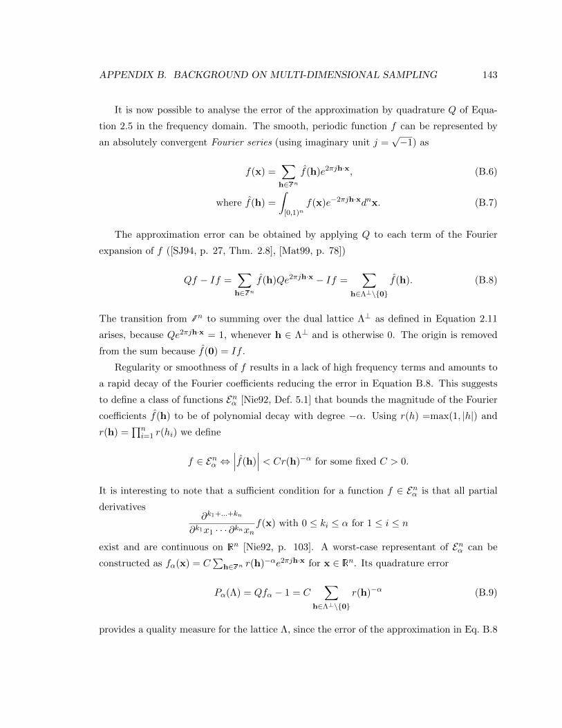
APPENDIX B. BACKGROUND ON MULTI-DIMENSIONAL SAMPLING 143
It is now possible to analyse the error of the approximation by quadrature Q of Equa-
tion 2.5 in the frequency domain. The smooth, periodic function f can be represented by
an absolutely convergent Fourier series (using imaginary unit j =√−1) as
f(x) =∑
h∈Znf(h)e2πjh·x, (B.6)
where f(h) =
∫[0,1)n
f(x)e−2πjh·xdnx. (B.7)
The approximation error can be obtained by applying Q to each term of the Fourier
expansion of f ([SJ94, p. 27, Thm. 2.8], [Mat99, p. 78])
Qf − If =∑
h∈Znf(h)Qe2πjh·x − If =
∑h∈Λ⊥\0
f(h). (B.8)
The transition from Zn to summing over the dual lattice Λ⊥ as defined in Equation 2.11
arises, because Qe2πjh·x = 1, whenever h ∈ Λ⊥ and is otherwise 0. The origin is removed
from the sum because f(0) = If .
Regularity or smoothness of f results in a lack of high frequency terms and amounts to
a rapid decay of the Fourier coefficients reducing the error in Equation B.8. This suggests
to define a class of functions Enα [Nie92, Def. 5.1] that bounds the magnitude of the Fourier
coefficients f(h) to be of polynomial decay with degree −α. Using r(h) =max(1, |h|) and
r(h) =∏ni=1 r(hi) we define
f ∈ Enα ⇔∣∣∣f(h)
∣∣∣ < Cr(h)−α for some fixed C > 0.
It is interesting to note that a sufficient condition for a function f ∈ Enα is that all partial
derivatives∂k1+...+kn
∂k1x1 · · · ∂knxnf(x) with 0 ≤ ki ≤ α for 1 ≤ i ≤ n
exist and are continuous on Rn [Nie92, p. 103]. A worst-case representant of Enα can be
constructed as fα(x) = C∑
h∈Zn r(h)−αe2πjh·x for x ∈ Rn. Its quadrature error
Pα(Λ) = Qfα − 1 = C∑
h∈Λ⊥\0
r(h)−α (B.9)
provides a quality measure for the lattice Λ, since the error of the approximation in Eq. B.8
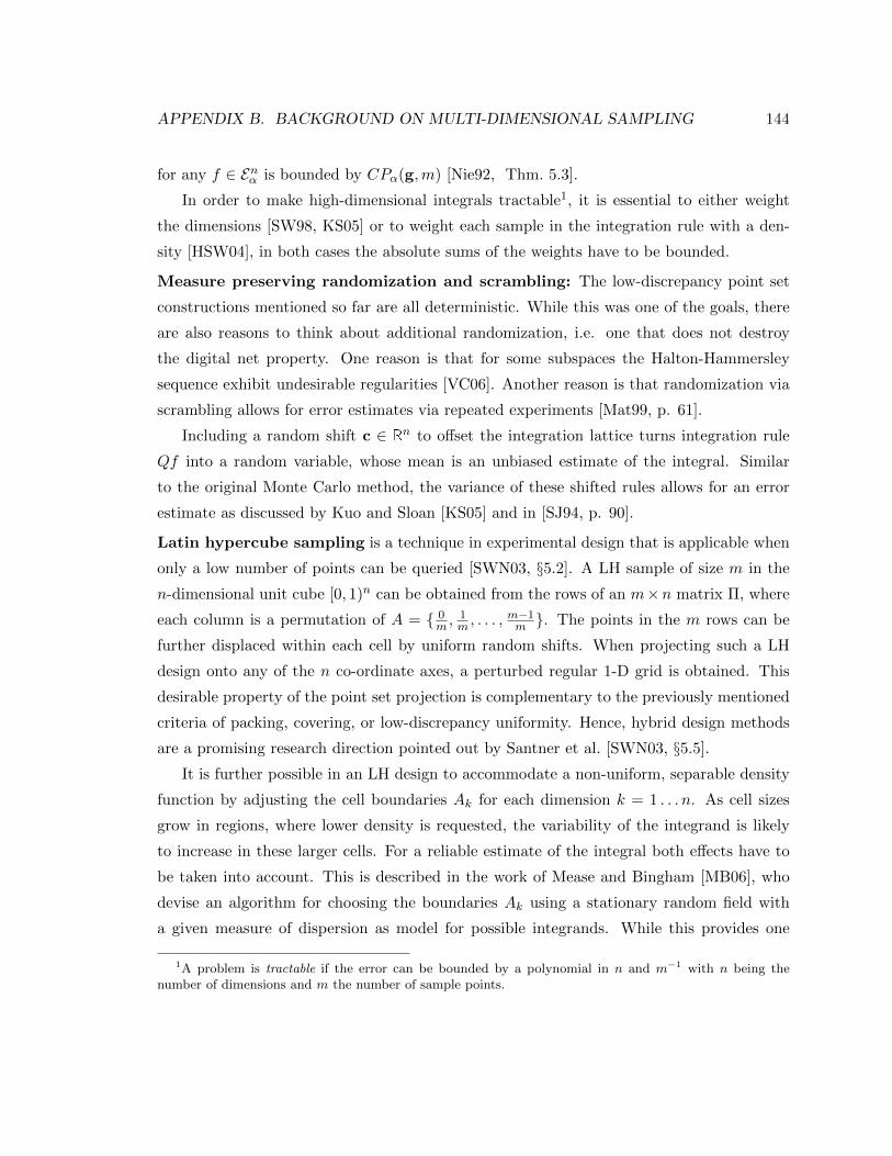
APPENDIX B. BACKGROUND ON MULTI-DIMENSIONAL SAMPLING 144
for any f ∈ Enα is bounded by CPα(g,m) [Nie92, Thm. 5.3].
In order to make high-dimensional integrals tractable1, it is essential to either weight
the dimensions [SW98, KS05] or to weight each sample in the integration rule with a den-
sity [HSW04], in both cases the absolute sums of the weights have to be bounded.
Measure preserving randomization and scrambling: The low-discrepancy point set
constructions mentioned so far are all deterministic. While this was one of the goals, there
are also reasons to think about additional randomization, i.e. one that does not destroy
the digital net property. One reason is that for some subspaces the Halton-Hammersley
sequence exhibit undesirable regularities [VC06]. Another reason is that randomization via
scrambling allows for error estimates via repeated experiments [Mat99, p. 61].
Including a random shift c ∈ Rn to offset the integration lattice turns integration rule
Qf into a random variable, whose mean is an unbiased estimate of the integral. Similar
to the original Monte Carlo method, the variance of these shifted rules allows for an error
estimate as discussed by Kuo and Sloan [KS05] and in [SJ94, p. 90].
Latin hypercube sampling is a technique in experimental design that is applicable when
only a low number of points can be queried [SWN03, §5.2]. A LH sample of size m in the
n-dimensional unit cube [0, 1)n can be obtained from the rows of an m×n matrix Π, where
each column is a permutation of A = 0m ,
1m , . . . ,
m−1m . The points in the m rows can be
further displaced within each cell by uniform random shifts. When projecting such a LH
design onto any of the n co-ordinate axes, a perturbed regular 1-D grid is obtained. This
desirable property of the point set projection is complementary to the previously mentioned
criteria of packing, covering, or low-discrepancy uniformity. Hence, hybrid design methods
are a promising research direction pointed out by Santner et al. [SWN03, §5.5].
It is further possible in an LH design to accommodate a non-uniform, separable density
function by adjusting the cell boundaries Ak for each dimension k = 1 . . . n. As cell sizes
grow in regions, where lower density is requested, the variability of the integrand is likely
to increase in these larger cells. For a reliable estimate of the integral both effects have to
be taken into account. This is described in the work of Mease and Bingham [MB06], who
devise an algorithm for choosing the boundaries Ak using a stationary random field with
a given measure of dispersion as model for possible integrands. While this provides one
1A problem is tractable if the error can be bounded by a polynomial in n and m−1 with n being thenumber of dimensions and m the number of sample points.
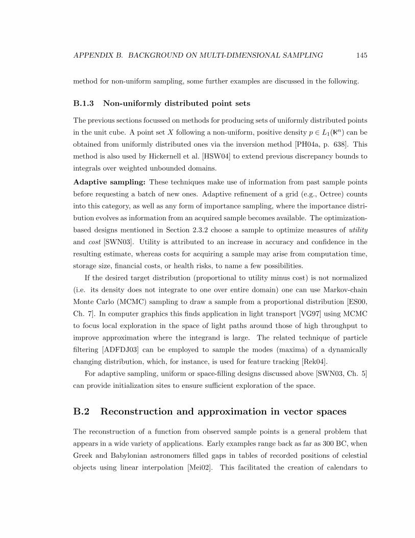
APPENDIX B. BACKGROUND ON MULTI-DIMENSIONAL SAMPLING 145
method for non-uniform sampling, some further examples are discussed in the following.
B.1.3 Non-uniformly distributed point sets
The previous sections focussed on methods for producing sets of uniformly distributed points
in the unit cube. A point set X following a non-uniform, positive density p ∈ L1(Rn) can be
obtained from uniformly distributed ones via the inversion method [PH04a, p. 638]. This
method is also used by Hickernell et al. [HSW04] to extend previous discrepancy bounds to
integrals over weighted unbounded domains.
Adaptive sampling: These techniques make use of information from past sample points
before requesting a batch of new ones. Adaptive refinement of a grid (e.g., Octree) counts
into this category, as well as any form of importance sampling, where the importance distri-
bution evolves as information from an acquired sample becomes available. The optimization-
based designs mentioned in Section 2.3.2 choose a sample to optimize measures of utility
and cost [SWN03]. Utility is attributed to an increase in accuracy and confidence in the
resulting estimate, whereas costs for acquiring a sample may arise from computation time,
storage size, financial costs, or health risks, to name a few possibilities.
If the desired target distribution (proportional to utility minus cost) is not normalized
(i.e. its density does not integrate to one over entire domain) one can use Markov-chain
Monte Carlo (MCMC) sampling to draw a sample from a proportional distribution [ES00,
Ch. 7]. In computer graphics this finds application in light transport [VG97] using MCMC
to focus local exploration in the space of light paths around those of high throughput to
improve approximation where the integrand is large. The related technique of particle
filtering [ADFDJ03] can be employed to sample the modes (maxima) of a dynamically
changing distribution, which, for instance, is used for feature tracking [Rek04].
For adaptive sampling, uniform or space-filling designs discussed above [SWN03, Ch. 5]
can provide initialization sites to ensure sufficient exploration of the space.
B.2 Reconstruction and approximation in vector spaces
The reconstruction of a function from observed sample points is a general problem that
appears in a wide variety of applications. Early examples range back as far as 300 BC, when
Greek and Babylonian astronomers filled gaps in tables of recorded positions of celestial
objects using linear interpolation [Mei02]. This facilitated the creation of calendars to
APPENDIX B. BACKGROUND ON MULTI-DIMENSIONAL SAMPLING 146
address down to earth questions, such as when to best till the fields or to bring in the
harvest. Making the leap into a more recent computational setting, function approximation,
as a way of fitting a model to given observations, is a core topic of machine learning and
statistics, where it is also referred to as regression or prediction ([Bis06, pp. 137],[SWN03,
pp. 49]). The signal processing perspective on sampling and reconstruction, used in the
following discussion, is laid out by Unser [Uns00].
Formally, one would like to reconstruct a function f : Rn → Rr from given observations
yk = f(xk) made at points of a sample X = xk ⊂ Rn with index k = 1 . . .m. In the
following, we will focus on the simple case n = r = 1 that is then extended to multi-
variate domains with n > 1. The case of multi-field functions with range dimension r > 1
is not explicitly considered here. A simple approach would be to treat every response
separately, while a combined treatment would allow to improve the representation using
vector quantization ideas of Section 2.3.1.1.
In order to compute function values f(x) at any previously unobserved position x 6∈ Xone has to generalize the information given for X to the entire domain of f . To do so,
some additional knowledge is required that can formally be expressed as membership of f
in a vector space F(Rn) of functions over the domain Rn. Modern signal processing ([BU99,
Uns00],[Gri02, Ch. 7],[CL09]) commonly takes F to be a Hilbert space equipped with an
inner product 〈·, ·〉 and properties as discussed in Appendix A.2. Such a space is complete
under the induced norm ‖f‖ =√〈f, f〉. It contains a countable set of basis functions ϕl
that can be scaled and summed to uniquely represent any function f ∈ F(Rn) as
f =∑l∈Z
clϕl. (B.10)
In computational practice one can only work with a finite number of parameters cl that
for l = 1 . . .m give a vector c ∈ Rm. The ϕl associated with these non-zero coefficients span
the reconstruction subspace V ⊆ F .
B.2.1 Projection, generalized interpolation, and best approximation
The mapping from F to V is performed by a linear approximation operator Q. A function f
in its range V can be represented faithfully and remains unchanged by another application
of Q, the implied property Q2f = Qf is defining for a projection. The best approximation
APPENDIX B. BACKGROUND ON MULTI-DIMENSIONAL SAMPLING 147
to f ∈ F in a subspace V ⊂ F is given by an orthogonal projection [Gri02, p. 185, 195]2.
The coefficients for the linear expansion in Equation B.10 can be obtained via func-
tionals λl that inherit the linearity from Q. Applied to continuous functions f they can
be implemented by an inner product with an analysis function ϕl as stated by the Riesz
representation theorem [CL09, p. 132] giving [CL09, p. 40]
cl = λl(f) = 〈ϕl, f〉. (B.11)
For any linear functional λ operating on subspace V one has the generalized interpolation
property λ(Qf) = λ(f) [CL09, p. 41]. Considering only one such functional is similar to the
integration problem of Section B.1. The classical notion of interpolation arises when using
point evaluation functionals λl(f) =∫f(x)δ(x− xl)dx = 〈δ(· − xl), f〉 = f(xl).
For perfect reconstruction the analysis functionals λl are bi-orthogonal to the basis func-
tions3 satisfying 〈ϕl, ϕk〉 = δ(k−l). If ϕl and ϕk do not fulfill the bi-orthogonality condition,
they can be made so by pre-filtering the measurements λl(f) [Uns00, BTU99]. A basis that
is bi-orthogonal to point evaluation functionals of the xk ∈ X is said to be a cardinal basis
for X. In this case the coefficients in Equation B.10 are simply given by the function values
cl = f(xl), corresponding to the standard notion of interpolation.
B.2.2 Determining the parameters for an interpolating function
The method to obtain coefficients via Equation B.11 is useful for theoretical understanding,
but in practise a complete description of f to compute the inner product with the analysis
filter is not available. If point samples of f are given, note that the parameters of an
interpolating approximant fc have to obey the equation system
f = Ac, (B.12)
2To see that an orthogonal projector Q maps a point x ∈ F to the closest point v in its range V, use thePythagorean Law‖x− v‖2 = ‖(x−Qx) + (Qx− v)‖2 = ‖x−Qx‖2 + ‖Qx− v‖2 ≥ ‖x−Qx‖2 [CL09, p. 210]. The Pythagoreanlaw holds, since 〈x + y, x + y〉 = 〈x, x〉 + 〈x, y〉 + 〈y, x〉 + 〈y, y〉 = 〈x, x〉 + 〈y, y〉, if x and y are orthogonal[Gri02, p. 179].
3With ϕk being a basis for V one can write∑l∈Z δ(k − l)ϕl = ϕk = Qϕk =
∑l∈Z λl(ϕk)ϕl. The
coefficients on the left and the right of this unique expansion can be identified, giving the bi-orthogonalityλl(ϕk) = δ(k − l).
APPENDIX B. BACKGROUND ON MULTI-DIMENSIONAL SAMPLING 148
where f contains the function values f(xk) for k = 1 . . .m and each row of the interpolation
matrix A ∈ Rm×n ([CL09, p. 4]; a.k.a. design matrix [SWN03, p. 54]) picks up values of
a basis function ϕl at the sample points Ak,l = ϕl(xk). The vector c of n coefficients can
be solved for uniquely only if matrix A is non-singular. If X has more points than there
are basis functions (m > n), Equation B.12 is an over-determined system. In this case, one
can still ask for c to minimize the 2-norm error argminc‖f − fc‖. A solution for this least
squares problem can be obtained as c = A+f using the pseudo-inverse [Bis06, p. 142]
A+ = (ATA)−1AT (B.13)
that performs an orthogonal projection onto the range of A [TI97, p. 81].
The form of matrix A is determined by the choice of basis ϕl and sample point
positions xk. The choices discussed in the following impose structure on A, such as
identity, triangular, Toeplitz, or symmetric positive definiteness and make it easier to solve
for the coefficients in Equation B.12.
Cardinal basis: Such a basis obeys ϕl(xk) = δ(l − k) for all xk in a sample X. This
turns A into an identity matrix and the coefficients in the expansion of Equation B.10
become cl = f(xl). On the real line the Lagrange polynomials ϕl(x) =∏nk=1k 6=l
x−xlxk−xl fulfill
this property and span the space∏n−1(R) of polynomials of degree n − 1 [CL09, p. 11].
One can extend these polynomials for interpolation on Rn by replacing the measure of
distance φ(x, y) = x− y in enumerator and denominator by other ones, such as the 2-norm
φ(x,y) = ‖x− y‖ or any metric φ(x,y) = d(x,y) [CL09, p. 62].
Triangular: Another approach is given by Newton’s polynomials, where a polynomial ϕl
associated with xl has its zeros at all xk for k < l. Hence, A turns into a triangular matrix
that can be solved via back substitution [CL09, p. 57].
Toeplitz: If the basis functions are shift-invariant, i.e. translates of a fixed function ϕ(x−xl) = ϕl(x) with a set of shift vectors that have translational group structure (i.e. X = xlis a lattice as defined in Section 2.3.1.3) [CL09, p. 71], then the columns of A can be ordered
to give constant diagonals, which is also referred to as Toeplitz matrix [Sta02, pp. 50]. Such
a matrix A performs a discrete convolution on c. Hence, for non-cardinal ϕl one can
obtain coefficients for an interpolating fc by inverse filtering of vector f [BTU99]. The
computational efficiency of being able to perform multiplication of a matrix of this type via
a convolution provides a strong application case for lattices for function reconstruction.
APPENDIX B. BACKGROUND ON MULTI-DIMENSIONAL SAMPLING 149
Symmetric, positive definite: The Schoenberg interpolation theorem [CL09, pp. 101]
states that a positive definite (and thus invertible) matrix A for radially symmetric basis
functions (RBF) ϕl(x) = h(‖x−xl‖2) can be formed with any completely monotone4 func-
tion h. Its orthogonal set of eigenvectors can be obtained via the Cholesky decomposition.
B.2.3 Perfect reconstruction and approximation
Perfect reconstruction is possible, if f lies in the finite dimensional reconstruction subspace
V. Shannon’s sampling theorem states that a function f with band-limit ω, i.e. f(ω) = 0
whenever |ω| > ω, can be perfectly reconstructed from sample points taken at regular
distance T = xk − xk−1 = π/ω. It involves a classical shift-invariant choice of basis on the
real line with generator ϕ(x) = T · sinc(x/T ), where sinc(x) = sin(πx)/πx, which is cardinal
for regularly spaced point samples and spans the space of band-limited functions [Sha49,
Uns00]. Interpolation in general shift-invariant spaces (i.e. φ 6= sinc) amounts to an oblique
projection, because the δ point evaluation functionals and the reconstruction filter do not
span the same space [Uns00, Sec. III-C].
Approximation error kernel: The approximation error in the general framework of
Hilbert space projections is discussed by Blu and Unser [BU99], who devise a quantitative
method of estimating the L2 approximation error ‖f − Qf‖2 of the operator defined in
Section B.2.1 as
εf (T ) =1
2π
∫ ∣∣∣f(ω)∣∣∣2Eϕ,ϕ(Tω)dω, (B.14)
where the error kernel E depends on analysis and synthesis filters ϕ and ϕ only
Eϕ,ϕ(Tω) =∣∣∣1− ˆϕ(ω)∗ϕ
∣∣∣2 +∣∣∣ ˆϕ(ω)
∣∣∣2∑n6=0
|ϕ(ω + 2nπ)|2 . (B.15)
The extension of Shannon’s theorem, mentioned at the beginning of this section, to
multi-dimensional domains has analog properties to the one dimensional case, where the
sampling distance T is reciprocal to the maximum frequency ω. In the multi-dimensional
version, provided by Petersen [PM62], a signal sampled on a lattice Λ has a frequency
domain representation on the dual lattice Λ⊥ (defined in Equation 2.11).
Using Hilbert space abstraction to model second order stationary random processes
4Complete monotonicity of f means 1. f ∈ C[0,∞), 2. f ∈ C∞(0,∞), 3. (−1)kf (k)(t) ≥ 0 for t > 0, k =0, 1, . . . .

APPENDIX B. BACKGROUND ON MULTI-DIMENSIONAL SAMPLING 150
Kunsch et al. [KAH05] derive an expression for the reconstruction error. Their results show
that for high-rate sampling of random fields, which corresponds to a wide, monotonously
decreasing correlation function, the lattice that maximizes the packing radius of the dual
lattice is favourable. Hence, for these high-rate sampling conditions in 3D the BCC lattice
provides an optimal choice, since it has the optimally packed FCC lattice as dual. For low
sampling rate cases they obtain a result that is similar to Johnson et al. [JMY90]. Corre-
sponding to a low correlation among adjacent sample points, the lowest average estimation
error in this setting is achieved when sampling with an optimal packing lattice. In R3 an
optimal choice is given by the FCC lattice.

Bibliography
[AB06] Ch.D. Aliprantis and K.C. Border. Infinite Dimensional Analysis - AHitchiker’s Guide. Springer, 2006.
[ABD10] A. Adams, J. Baek, and A. Davis. Fast high-dimensional filtering using thepermutohedral lattice. Computer Graphics Forum: Eurographics Symposiumon Rendering, May 2010.
[Abd11] Sareh Nabi Abdolyousefi. Equilibria of a nonlocal model for biological ag-gregations: Linear stability and bifurcation studies. Master’s thesis, Dept. ofMathematic, Simon Fraser University, 2011.
[ACM02] S. Azizi, D. Cochran, and J. N. McDonald. Reproducing kernel structure andsampling on time-warped spaces with application to warped wavelets. IEEETrans. on Information Theory, 48(3):789–790, March 2002.
[ADFDJ03] C. Andrieu, N. De Freitas, A. Doucet, and M.I. Jordan. An introduction toMCMC for machine learning. Machine learning, 50(1-2):5–43, 2003.
[AEVZ02] E. Agrell, T. Eriksson, A. Vardy, and K. Zeger. Closest point search in lattices.Information Theory, IEEE Transactions on, 48(8):2201–2214, August 2002.
[Ale65] P. Alexandroff. Elementary concepts of topology. Ungar publishing, 1965.
[ARC05] Alfie Abdul-Rahman and Min Chen. Spectral volume rendering based on theKubelka-Munk theory. Computer Graphics Forum, 24(3):413–422, 2005.
[BAZT04] S. Bergner, S. Al-Zubi, and K. D. Tonnies. Deformable structural models.In Proc. of IEEE Intl. Conf. on Image Processing (ICIP), pages 1875–1878,October 2004.
[BBPD08] J. Blaas, C. Botha, F. Post, and TU Delft. Extensions of Parallel Coordinatesfor Interactive Exploration of Large Multi-Timepoint Data Sets. IEEE Trans.on Visualization and Computer Graphics, 14(6):1436–1451, 2008.
[BCKM11] Steven Bergner, Matthew Crider, Arthur E. Kirkpatrick, and Torsten Moller.Mixing board versus mouse interaction in value adjustment tasks, Oct 2011.arXiv:1110.2520.
[BCM05] A. Buades, B. Coll, and J. Morel. A non-local algorithm for image denois-ing. In IEEE Computer Society Conference on Computer Vision and PatternRecognition, volume 2, page 60, 2005.
151
BIBLIOGRAPHY 152
[BDM09] S. Bergner, M. S. Drew, and T. Moller. A tool to create illuminant andreflectance spectra for light-driven graphics and visualization. ACM Trans.Graph., 28(1):(article 5), 2009.
[Bel61] R. E. Bellman. Adaptive Control Processes: A Guided Tour. Princeton Uni-versity Press, 1961.
[Ber03] S. Bergner. Structural deformable models for robust object recognition. Mas-ter’s thesis, Dept. of Simulation and Graphics, Otto-von-Guericke University,2003. http://wwwisg.cs.uni-magdeburg.de/bv/theses/thesis bergner.pdf.
[BFG08] E. Brochu, N. De Freitas, and A. Ghosh. Active preference learning withdiscrete choice data. In J.C. Platt, D. Koller, Y. Singer, and S. Roweis,editors, Advances in Neural Information Processing Systems 20, pages 409–416. MIT Press, Cambridge, MA, 2008.
[BG04] H.J. Bungartz and M. Griebel. Sparse grids. Acta Numerica, 13:147–269,2004.
[Bis06] Ch. M. Bishop. Pattern Recognition and Machine Learning. Springer, August2006.
[BJ95] R. G. Baraniuk and D. L. Jones. Unitary equivalence: a new twist on signalprocessing. IEEE Trans. on Signal Processing, 43(10):2269–2282, October1995.
[BK95] V. Bhatt and J. Koechling. Partitioning the parameter space according todifferent behaviors during three-dimensional impacts. Journal of applied me-chanics, 62:740, 1995.
[BM10] S. Bruckner and T. Moller. Result-driven exploration of simulation parameterspaces for visual effects design. IEEE Trans. on Vis. and Comp. Graph. (Proc.Visualization / Info. Vis. 2010), 16:1467–1475, Nov.-Dec. 2010.
[BMDF02] Steven Bergner, Torsten Moller, Mark S. Drew, and Graham D. Finlayson.Interactive spectral volume rendering. In Proc. of IEEE Visualization 2002,pages 101–108, October 2002.
[BMTD05] Steven Bergner, Torsten Moller, Melanie Tory, and Mark S. Drew. A practicalapproach to spectral volume rendering. IEEE Trans. on Vis. and Comp.Graphics, 11(2):207–216, March/April 2005.
[BMWM06] Steven Bergner, Torsten Moller, Daniel Weiskopf, and David J. Muraki. Aspectral analysis of function composition and its implications for sampling indirect volume visualization. IEEE Transactions on Visualization and Com-puter Graphics (Proceedings Visualization / Information Visualization 2006),12(5):1353–1360, Sep.-Oct 2006.
[BPFG11] W. Berger, H. Piringer, P. Filzmoser, and E. Groller. Uncertainty-aware ex-ploration of continuous parameter spaces using multivariate prediction. Com-puter Graphics Forum, 30(3):911–920, 2011.
BIBLIOGRAPHY 153
[Bre02] P. Bremaud. Mathematical principles of signal processing: Fourier andwavelet analysis. Springer Verlag, 2002.
[BSC+06] J. Buhl, D.J.T. Sumpter, I.D. Couzin, J.J. Hale, E. Despland, E.R. Miller,and S.J. Simpson. From disorder to order in marching locusts. Science,312(5778):1402, 2006.
[BSD09] M. Balzer, T. Schlomer, and O. Deussen. Capacity-Constrained Point Distri-butions: A Variant of Lloyd’s Method. ACM Trans. on Graphics (Proc. ofSIGGRAPH), 28(3):(No. 86), 2009.
[BSNA+11] Steven Bergner, Michael Sedlmair, Sareh Nabi-Abdolyousefi, Ahmed Saad,and Torsten Moller. Paraglide: Interactive Parameter Space Partitioning forComputer Simulations, Sep 2011. Submitted to IEEE Trans. on Vis. andComp. Graphics, Sep. 2011.
[BTU99] T. Blu, P. Thevenaz, and M. Unser. Generalized interpolation: Higher qualityat no additional cost. In Intl. Conf. on Image Proc. (ICIP)’99, volume III,pages 667–671, 1999.
[BU99] T. Blu and M. Unser. Quantitative Fourier analysis of approximation tech-niques. I. Interpolators and projectors. IEEE Trans. on Signal Processing,47(10):2783–2795, 1999.
[BVBM09] S. Bergner, D. Van De Ville, T. Blu, and T. Moller. On sampling latticeswith similarity scaling relationships. In Proc. of SAMPTA 2009, May 2009.
[BW08] S. Bachtaler and D. Weiskopf. Continuous scatterplots. IEEE Trans.on Comp. Graphics and Visualization - Proc. of IEEE Visualization 2008,14(6):(8 pages), 2008.
[BWB09] I. Buchan, J. Winn, and Ch. Bishop. A Unified Modeling Approach to Data-Intensive Healthcare. In A.J.G. Hey, S. Tansley, and K.M. Tolle, editors, Thefourth paradigm: data-intensive scientific discovery, chapter 13, pages 91–97.Microsoft Research Redmond, WA, 2009.
[BZS+07] Pravin Bhat, C. Lawrence Zitnick, Noah Snavely, Aseem Agarwala, ManeeshAgrawala, Brian Curless, Michael Cohen, and Sing Bing Kang. Using pho-tographs to enhance videos of a static scene. In Jan Kautz and Sumanta Pat-tanaik, editors, Rendering Techniques 2007 (Proceedings Eurographics Sym-posium on Rendering), pages 327–338. Eurographics, June 2007.
[CB09] J. Cortes and F. Bullo. Nonsmooth Coordination and Geometric Optimiza-tion via Distributed Dynamical Systems. SIAM Review, 51:163, 2009.
[CBS+07] M. Crider, S. Bergner, T. Smyth, A.T. Kirkpatrick, and T. Moller. A mixingboard interface for graphics and visualization applications. In Proc. GraphicsInterface 2007, pages 87–94, Montreal, QC, 2007. ACM.
[Che10] S.V. Chekanov. Scientific data analysis using Jython Scripting and Java.Advanced Information And Knowledge Processing, page 440, 2010.
BIBLIOGRAPHY 154
[CJ10] M. Chen and H. Jaenicke. An information-theoretic framework for visu-alization. Visualization and Computer Graphics, IEEE Transactions on,16(6):1206–1215, 2010.
[CK95] P.R. Cohen and R. Kohavi. Empirical methods for artificial intelligence,volume 55. MIT press, 1995.
[CKPW07] Paul Chang, Gwang-Soo Kim, Keith Promislow, and Brian Wetton. Reduceddimensional computational models of polymer electrolyte membrane fuel cellstacks. J. Comput. Phys., 223(2):797–821, 2007.
[CL09] W. Cheney and W. Light. A Course in Approximation Theory. AMS, 2009.
[CM97] S.K. Card and J. Mackinlay. The structure of the information visualizationdesign space. In Proceedings of the 1997 IEEE Symposium on InformationVisualization (InfoVis’ 97), page 92, 1997.
[CPL85] J. Clark, M. Palmer, and P. Lawrence. A transformation method for thereconstruction of functions from nonuniformly spaced samples. IEEE Trans.on Acoustics, Speech, and Signal Processing, 33(5):1151–1165, October 1985.
[CS82] J.H. Conway and N.J.A. Sloane. Voronoi regions of lattices, second momentsof polytopes, and quantization. IEEE Trans. on Information Theory, IT-28(2):211–226, March 1982.
[CS85] J. Conway and N. Sloane. A lower bound on the average error of vector quan-tizers (Corresp.). Information Theory, IEEE Transactions on, 31(1):106–109,1985.
[CS99] J.H. Conway and N.J.A. Sloane. Sphere Packings, Lattices and Groups. – 3rded. Springer, 1999.
[CSK03] B. Csebfalvi and L. Szirmay-Kalos. Monte carlo volume rendering. In Proc.IEEE Visualization’03, pages 449–456, 2003.
[Dal93] S. Daly. The visible differences predictor: an algorithm for the assessment ofimage fidelity. Digital images and human vision, 4, 1993.
[DCWP02] Kate Devlin, Alan Chalmers, Alexander Wilkie, and Werner Purgathofer.Star: Tone reproduction and physically based spectral rendering. In DieterFellner and Roberto Scopignio, editors, State of the Art Reports, Eurographics2002, pages 101–123. The Eurographics Association, September 2002.
[DEJ06] Q. Du, M. Emelianenko, and L. Ju. Convergence of the Lloyd algorithm forcomputing centroidal Voronoi tessellations. CONVERGENCE, 44(1):102–119, 2006.
[DF92] Mark S. Drew and Brian V. Funt. Natural metamers. CVGIP:Image Under-standing, 56:139–151, 1992.
[DF03] Mark S. Drew and Graham D. Finlayson. Multispectral processing withoutspectra. J. Opt. Soc. Am. A, 20(7):1181–1193, July 2003.

BIBLIOGRAPHY 155
[DGH03] H. Doleisch, M. Gasser, and H. Hauser. Interactive feature specification forfocus+ context visualization of complex simulation data. In Proc. of the sym-posium on data visualisation 2003, pages 239–248. Eurographics Association,2003.
[DHL+98] O. Deussen, P. Hanrahan, B. Lintermann, R. Mech, M. Pharr, andP. Prusinkiewicz. Realistic modeling and rendering of plant ecosystems. InProceedings of the 25th annual conference on Computer graphics and inter-active techniques, pages 275–286. ACM, 1998.
[Dic45] L. R. Dice. Measures of the amount of ecologic association between species.Ecology, 26(3):297–302, 1945.
[DJ06] C. Donner and H. W. Jensen. A spectral shading model for human skin. InRendering Techniques (Proc. of the Eurographics Symp. on Rendering), pages409–417, 2006.
[dSB04] S. dos Santos and K. Brodlie. Gaining understanding of multivariate and mul-tidimensional data through visualization. Computers & Graphics, 28(3):311–325, 2004.
[Dud79] R. Duda. The origins of the concept of dimension. Colloq. Math., 42:95–110,1979.
[EDM09] A. Entezari, R. Dyer, and T. Moller. From Sphere Packing to the Theory ofOptimal Lattice Sampling, page (29 pages). Springer, 2009.
[EKE01a] K. Engel, M. Kraus, and T. Ertl. High-quality pre-integrated volume render-ing using hardware-accelerated pixel shading. In Eurographics / SIGGRAPHWorkshop on Graphics Hardware ’01, 2001.
[EKE01b] K. Engel, M. Kraus, and T. Ertl. High-quality pre-integrated volume render-ing using hardware-accelerated pixel shading. In Eurographics / SIGGRAPHWorkshop on Graphics Hardware 2001, pages 9–16, 2001.
[EMV04] A. Entezari, T. Moller, and J. Vaisey. Subsampling matrices for wavelet de-compositions on body centered cubic lattices. IEEE Signal Processing Letters(SPL), 11(9):733–735, Sept. 2004.
[Ent07] Alireza Entezari. Optimal sampling lattices and trivariate box splines. PhDthesis, Simon Fraser Univsersity, 2007.
[ERT05] S. Esedoglu, S. Ruuth, and R. Tsai. Threshold dynamics for shape recon-struction and disocclusion. In Image Processing, 2005. ICIP 2005. IEEEInternational Conference on, volume 2, pages II–502. IEEE, 2005.
[ES00] M. Evans and T. Swartz. Approximating integrals via Monte Carlo and de-terministic methods. Oxford University Press, USA, 2000.
[FCSW99] J. Farrell, J. Cupitt, D. Saunders, and B.A. Wandell. Estimating spectralreflectances of digital artwork. In Chiba Conference of Multispectral Imaging,1999.
BIBLIOGRAPHY 156
[FdOL03] M.C. Ferreira de Oliveira and H. Levkowitz. From visual data exploration tovisual data mining: A survey. IEEE Trans. on Visualization and ComputerGraphics, 9(3):378–394, 2003.
[FE10] R. C. Fetecau and R. Eftimie. An investigation of a nonlocal hyperbolic modelfor self-organization of biological groups. J. Math. Biol., 61(4):545–579, 2010.
[Fra07] D. Francois. High-dimensional data analysis: optimal metrics and featureselection. PhD thesis, Universite catholique de Louvain, 2007.
[GC08] A. Guillot and C. Collet. Construction of the motor imagery integrativemodel in sport: a review and theoretical investigation of motor imagery use.International Review of Sport and Exercise Psychology, 1(1):31–44, 2008.
[GH87] M. Greenacre and T. Hastie. The geometric interpretation of correspondenceanalysis. J. of the Am. Stat. Assoc., 82(398):437–447, June 1987.
[Gil93] W.J. Gilbert. Bricklaying and the hermite normal form. American Mathe-matical Monthly, 100:242–245, March 1993.
[GJ79] M.R. Garey and D.S. Johnson. Computers and intractability: A Guide to theTheory of NP-Completeness, volume 174. Freeman, San Francisco, CA, 1979.
[Gla89] A.S. Glassner. How to derive a spectrum from an RGB triplet. ComputerGraphics and Applications, IEEE, 9(4):95–99, July 1989.
[Gla95] A. S. Glassner. Principles of digital image synthesis. Morgan Kaufman Pub-lishers, 1995.
[GMN94] J.S. Gondek, G.W. Meyer, and J.G. Newman. Wavelength dependent re-flectance functions. In Proc. SIGGRAPH 1994, pages 213–220, Orlando, FL,1994. ACM.
[Gol10] E.B. Goldstein. Encyclopedia of perception, volume 1+2. Sage Publications,Inc, 2010.
[Gra06] L. Grady. Random walks for image segmentation. IEEE Trans. on PatternAnalysis and Mach. Intelligence, 28(11):1768–1783, Nov. 2006.
[Gri02] D. H. Griffel. Applied Functional Analysis. Dover, 2002.
[Gri06] M. Griebel. Sparse grids and related approximation schemes for higher di-mensional problems. In L. Pardo, A. Pinkus, E. Suli, and M.J. Todd, editors,Foundations of Computational Mathematics (FoCM05), Santander, pages106–161. Cambridge University Press, 2006.
[HA02] F.A. Hamprecht and E. Agrell. Exploring a space of materials: Spatial sam-pling design and subset selection. Experimental Design for Combinatorialand High Throughput Materials Development. John Wiley & Sons, 2002.

BIBLIOGRAPHY 157
[HA06] J. Heer and M. Agrawala. Software design patterns for information visualiza-tion. IEEE Trans. on Visualization and Computer Graphics, 12(5):853–860,2006.
[Han05] K. M. Hanson. Halftoning and Quasi-Monte Carlo. In K. M. Hanson andF. M. Hemez, editors, Sensitivity Analysis of Model Output, pages 430–442,Los Alamos Research Library, 2005.
[HB03] Mark A. Harrower and Cynthia A. Brewer. Colorbrewer.org: An online toolfor selecting color schemes for maps. The Cartographic Journal, 40(1):27–37,2003. http://www.colorbrewer.org.
[HE03] M. Hopf and T. Ertl. Hierarchical splatting of scattered data. In Proceed-ings of the 14th IEEE Visualization 2003 (VIS’03). IEEE Computer SocietyWashington, DC, USA, 2003.
[HHS94] H.C. Hege, T. Hollerer, and D. Stalling. Volume Rendering, MathematicalModels and Algorithmic Aspects. Technical report, TR 93-7, Konrad-Zuse-Zentrum fur Informationstechnik Berlin, 1994.
[Hil91] D. Hilbert. Uber die stetige Abbildung einer Linie auf ein Flachenstuck.Math. Ann., 38:459–460, 1891.
[Him04] Johan Himberg. From insights to innovations: datamining, visualization, anduser interfaces. PhD thesis, Helsinki University of Technology, 2004.
[HK93] Pat Hanrahan and Wolfgang Krueger. Reflection from layered surfaces dueto subsurface scattering. In Proceedings of ACM SIGGRAPH 1993, Com-puter Graphics Proceedings, Annual Conference Series, pages 165–174. ACMSIGGRAPH, August 1993.
[HM90] R.B. Haber and D.A. McNabb. Visualization idioms: A conceptual model forscientific visualization systems. Visualization in scientific computing, pages74–93, 1990.
[Hol06] R. Holbrey. Data reduction algorithms for data mining and visualization.Technical report, University of Leeds/Edinburgh, 2006.
[HS88] S.G. Hart and L.E. Staveland. Development of NASA-TLX (Task Load In-dex): Results of empirical and theoretical research. Human mental workload,1:139–183, 1988.
[HSW04] F.J. Hickernell, I.H. Sloan, and G.W. Wasilkowski. On tractability of weightedintegration over bounded and unbounded regions in Rs. Mathematics of Com-putation, 73:1885–1902, 2004.
[IMI+10] S. Ingram, T. Munzner, V. Irvine, M. Tory, S. Bergner, and T. Moller. Dim-Stiller: Workflows for dimensional analysis and reduction. In Visual Analyt-ics Science and Technology (VAST), 2010 IEEE Symposium on, pages 3–10.IEEE, 2010.
BIBLIOGRAPHY 158
[IMO09] S. Ingram, T. Munzner, and M. Olano. Glimmer: Multilevel MDS on theGPU. IEEE Trans. on Visualization and Computer Graphics, pages 249–261, 2009.
[JBS08] H. Janicke, M. Bottinger, and G. Scheuermann. Brushing of Attribute Cloudsfor the Visualization of Multivariate Data. IEEE Trans. on Visualization andComputer Graphics, 14(6):1459–1466, 2008.
[JF99] G.M. Johnson and M.D. Fairchild. Full-spectral color calculations inrealistic image synthesis. Computer Graphics and Applications, 19(4:July/August):47–53, 1999.
[JMY90] M.E. Johnson, L.M. Moore, and D. Ylvisaker. Minimax and maximin distancedesigns. Journal of Statistical Planning and Inference, 26(2):131–148, 1990.
[JSW98] D.R. Jones, M. Schonlau, and W.J. Welch. Efficient global optimization ofexpensive black-box functions. Journal of Global Optimization, 13(4):455–492, 1998.
[KAH05] H.R. Kunsch, E. Agrell, and F.A. Hamprecht. Optimal lattices for sampling.Information Theory, IEEE Transactions on, 51(2):634–647, February 2005.
[KK02] T. Kollig and A. Keller. Efficient multidimensional sampling. ComputerGraphics Forum, 21(3):557–563, September 2002.
[KM07] G. Kelly and H. McCabe. Interactive city generation methods. In Intl. Conf.on Computer Graphics and Interactive Techniques: ACM SIGGRAPH 2007posters, San Diego, CA, 2007. ACM.
[KMP07] M. Kilian, N. J. Mitra, and H. Pottmann. Geometric modeling in shape space.ACM Transactions on Graphics, 26(3):1–8, 2007.
[Kni00] Gunter Knittel. The UltraVis system. In Proc. Symposium on Volume Visu-alization 2000, pages 71–79, 2000.
[KPH+03] J. Kniss, S. Premoze, Ch. Hansen, P. Shirley, and A. McPherson. A model forvolume lighting and modeling. IEEE Trans. on Visualization and ComputerGraphics 2003, 9(2):150–162, April-June 2003.
[Kra03] Martin Kraus. Direct Volume Visualization of Geometrically UnpleasantMeshes. PhD thesis, University of Stuttgart, 2003.
[KS05] F. Y. Kuo and I. H. Sloan. Lifting the curse of dimensionality. Notices Amer.Math. Soc., 52:1320–1328, 2005.
[KSBF10] J. Kietz, F. Serban, A. Bernstein, and S. Fischer. Data mining workflowtemplates for intelligent discovery assistance and auto-experimentation. InThird-Generation Data Mining: Towards Service-Oriented Knowledge Dis-covery SoKD, volume 10, pages 1–12, 2010.
BIBLIOGRAPHY 159
[KUMY10] J. Kronander, J. Unger, T. Moller, and A. Ynnerman. Estimation and mod-eling of actual numerical errors in volume rendering. Computer GraphicsForum, 29(3):893–902, 2010.
[KV92] J. Kovacevic and M. Vetterli. Nonseparable multidimensional perfect recon-struction filter banks and wavelet bases for Rn. Inf. Theory, IEEE Trans.on, 38(2), March 1992.
[KW03] Jens Kruger and Rudiger Westermann. Acceleration techniques for GPU-based volume rendering. In Proc. IEEE Visualization 2003, pages 287–292,2003.
[Law91] J. Lawrence. Polytope volume computation. Mathematics of Computation,57(195):259–271, 1991.
[LB05] E. Levina and P.J. Bickel. Maximum likelihood estimation of intrinsic dimen-sion. In L. K. Saul, Y. Weiss, and L. Bottou, editors, Advances in NIPS 17,2005.
[Lem09] C. Lemieux. Monte Carlo and Quasi-Monte Carlo Sampling. Springer Verlag,2009.
[LH91] D. Laur and P. Hanrahan. Hierarchical splatting: A progressive refinement al-gorithm for volume rendering. Computer Graphics (Proc. ACM SIGGRAPH’91), 25(4):285–288, 1991.
[LH98] J. Leydold and A. Hormann. A sweep-plane algorithm for generating randomtuples in simple polytopes. Mathematics of Computation, 67(224):1617–1635,Oct 1998.
[LHJ99] Eric LaMar, Bernd Hamann, and Kenneth I. Joy. Multiresolution techniquesfor interactive texture-based volume visualization. In Proc. IEEE Visualiza-tion 1999, pages 355–361, 1999.
[Llo82] S. Lloyd. Least squares quantization in PCM. IEEE Trans. on InformationTheory, 28(2):129–137, 1982.
[LMK03] Wei Li, Klaus Mueller, and Arie Kaufman. Empty space skipping and occlu-sion clipping for texture-based volume rendering. In Proc. IEEE Visualization2003, pages 317–324, 2003.
[LPC+00] Marc Levoy, Kari Pulli, Brian Curless, Szymon Rusinkiewicz, David Koller,Lucas Pereira, Matt Ginzton, Sean Anderson, James Davis, Jeremy Ginsberg,Jonathan Shade, and Duane Fulk. The digital michelangelo project: 3D scan-ning of large statues. In Proceedings of ACM SIGGRAPH 2000, ComputerGraphics Proceedings, Annual Conference Series, pages 131–144. ACM, July2000.
[LS02] F. Lutscher and A. Stevens. Emerging patterns in a hyperbolic model forlocally interacting cell systems. J. Nonlinear Sci., 12:619–640, 2002.

BIBLIOGRAPHY 160
[Lux07] U. Luxburg. A tutorial on spectral clustering. Statistics and Computing,17(4):395–416, 2007.
[MAB+97] J. Marks, B. Andalman, P. A. Beardsley, W. Freeman, S. Gibson, J. Hod-gins, T. Kang, B. Mirtich, H. Pfister, W. Ruml, K. Ryall, J. Seims, andS. Shieber. Design galleries: A general approach to setting parameters forcomputer graphics and animation. In SIGGRAPH ’97, pages 389–400. ACMPress, 1997.
[Mat99] J. Matousek. Geometric Discrepancy - An illustrated guide. Springer, 1999.
[Mat02] J. Matousek. Lectures on Discrete Geometry. Springer, 2002.
[MB06] D. Mease and D. Bingham. Latin hyperrectangle sampling for computerexperiments. Technometrics, 48(4):467–477, 2006.
[McM70] P. McMullen. Polytopes with centrally symmetric faces. Israel Journal ofMathematics, 8(2), June 1970.
[Mei02] E. Meijering. A chronology of interpolation: From ancient astronomy tomodern signal and image processing. Proc. of the IEEE, pages 319–342,2002.
[MH07] Ch. Mcintosh and G. Hamarneh. Is a single energy functional sufficient?Adaptive energy functionals and automatic initialization. Proc. MICCAI,Part II, 4792:503–510, 2007.
[MM07] J.I. Mulero-Martınez. Functions bandlimited in frequency are free of the curseof dimensionality. Neurocomputing, 70(7-9):1439–1452, 2007.
[MMC99] K. Mueller, T. Moller, and R. Crawfis. Splatting without the blur. In Proc.Visualization’99, pages 363–371, 1999.
[MMMY97] T. Moller, R. Machiraju, K. Mueller, and R. Yagel. Evaluation and design offilters using a taylor series expansion. Visualization and Computer Graphics,IEEE Transactions on, 3(2):184–199, 1997.
[MPBM03] Wojciech Matusik, Hanspeter Pfister, Matthew Brand, and Leonard McMil-lan. A data-driven reflectance model. ACM Transactions on Graphics,22(3):759–769, July 2003.
[Mun09] T. Munzner. A nested model for visualization design and validation. IEEETrans. on Visualization and Computer Graphics, 15(6):921–928, 2009.
[Mun12] Tamara Munzner. Information Visualization: Principles, Methods, and Prac-tice. AK Peters, 2012. (pre-publication draft, to appear).
[MvWvL99] J.D. Mulder, J.J. van Wijk, and R. van Liere. A survey of computationalsteering environments. Future Generation Computer Systems, 15(1):119 –129, 1999.

BIBLIOGRAPHY 161
[MW92] David H. Marimont and Brian A. Wandell. Linear models of surface andilluminant spectra. J. Opt. Soc. Am. A, 11:1905–1913, 1992.
[MW95] A.R. Martin and M.O. Ward. High dimensional brushing for interactive ex-ploration of multivariate data. In Proc. of 6th Conference on Visualization’95, pages 271–278. IEEE Computer Society, 1995.
[MWK+06] I. Mierswa, M. Wurst, R. Klinkenberg, M. Scholz, and T. Euler. YALE:Rapid prototyping for complex data mining tasks. In Proc. of the 12th ACMSIGKDD Intl. Conference on Knowledge Discovery and Data Mining, pages935–940. ACM, 2006.
[New72] M. Newman. Integral Matrices. Academic Press, 1972.
[NH06] M. Novotny and H. Hauser. Outlier-preserving focus+context visualizationin parallel coordinates. IEEE Trans. on Comp. Graphics and Visualization -Proc. of IEEE Visualization 2006, 12(5):893–900, 2006.
[Nie92] H. Niederreiter. Random Number Generation and Quasi-Monte Carlo Meth-ods. Society for Industrial and Applied Mathematics, 1992.
[NvdVS00] Herke Jan Noordmans, Hans T.M. van der Voort, and Arnold W.M. Smeul-ders. Spectral volume rendering. In IEEE Transactions on Visualization andComputer Graphics, pages 196–207. IEEE Computer Society, 2000.
[Par99] J. K. Parrish. Using behavior and ecology to exploit schooling fishes. Environ.Biol. Fish., 55:157–181, 1999.
[PBCR11] A.J. Pretorius, M.A.P. Bray, A.E. Carpenter, and R.A. Ruddle. Visualizationof parameter space for image analysis. IEEE Trans. on Vis. and comp. Graph.,page In Press., 2011.
[PBMW99] L. Page, S. Brin, R. Motwani, and T. Winograd. The pagerank citationranking: Bringing order to the web. 1999.
[Pee93] Mark S. Peercy. Linear color representations for full spectral rendering. InComputer Graphics (SIGGRAPH ’93), pages 191–198. ACM, 1993.
[PH04a] M. Pharr and G. Humphreys. Physically Based Rendering: From Theory toImplementation. Morgan Kaufmann, 2004.
[PH04b] Matt Pharr and Greg Humphreys. Physically based rendering. Elsevier, SanFrancisco, CA, 2004.
[PH04c] Matt Pharr and Greg Humphreys. Physically Based Rendering: From Theoryto Implementation. Morgan Kaufmann, August 2004.
[PH10] K. Pothkow and H. Hege. Positional uncertainty of isocontours: Conditionanalysis and probabilistic measures. Visualization and Computer Graphics,IEEE Trans. on, 17(10):1393–1406, Nov 2010.

BIBLIOGRAPHY 162
[Phi03] G.M.A. Phillips. Interpolation and approximation by polynomials. Springer,2003.
[PKG99] M. Pollefeys, R. Koch, and L.V. Gool. Self-calibration and metric reconstruc-tion inspite of varying and unknown intrinsic camera parameters. Intl. J. ofComputer Vision, 32(1):7–25, 1999.
[PKNM06] M.A. Pitt, W. Kim, D.J. Navarro, and J.I. Myung. Global model analysis byparameter space partitioning. Psychological Review, 113(1):57, 2006.
[PM62] D.P. Petersen and D. Middleton. Sampling and reconstruction of wave-number-limited functions in n-dimensional euclidean spaces. Information andControl, 5:279–323, 1962.
[PVF05] R.M. Pillat, E.R.A. Valiati, and C.M.D.S. Freitas. Experimental study onevaluation of multidimensional information visualization techniques. In Proc.of the 2005 Latin American conf. on Human-computer interaction, pages 20–30. ACM, 2005.
[PZB95] Mark S. Peercy, Benjamin M. Zhu, and Daniel R. Baum. Interactive fullspectral rendering. In Proceedings of the 1995 Symposium on Interactive 3Dgraphics, pages 67–68. ACM Press, 1995.
[Rek04] I. Rekleitis. A particle filter tutorial for mobile robot localization. TechnicalReport TR-CIM-04-02, Centre for Intelligent Machines, McGill University,Montreal, Quebec, Canada, 2004.
[RGWE03] S. Roettger, S. Guthe, D. Weiskopf, and T. Ertl. Smart hardware-acceleratedvolume rendering. In Proc. EG/IEEE TCVG Symposium on VisualizationVisSym 2003, pages 231–238, 2003.
[SFCD99] Y. Sun, F.D. Fracchia, T.W. Calvert, and M.S. Drew. Deriving spectra fromcolors and rendering light interference. Computer Graphics and Applications,IEEE, 19(4):61–67, Jul/Aug 1999.
[SFD00] Yinlong Sun, F. David Fracchia, and Mark S. Drew. Rendering diamonds. InProc. WCGS 2000, pages 9–15, 2000.
[SG86] M. Sabin and R. Gray. Global convergence and empirical consistency ofthe generalized Lloyd algorithm. IEEE Transactions on Information Theory,32(2):148–155, 1986.
[Sha49] C.E. Shannon. Communication in the presence of noise. Proc. IRE, 37(1):10–21, 1949.
[SHMS08] A. Saad, G. Hamarneh, T. Moller, and B. Smith. Kinetic modeling basedprobabilistic segmentation for molecular images. Medical Image Computingand Computer-Assisted Intervention–MICCAI 2008, pages 244–252, 2008.
[SHT97] G. Sharma and H.J. H.J. Trussell. Figures of merit for color scanners. IEEETrans. Image Proc., 6(7):990–1001, July 1997.
BIBLIOGRAPHY 163
[SJ94] I.H. Sloan and S. Joe. Lattice methods for multiple integration. Oxford Uni-versity Press, 1994.
[SJ09] B. Spencer and MW Jones. Into the Blue: Better Caustics through PhotonRelaxation. Computer Graphics Forum, 28(2):319–328, 2009.
[SK00] M. Sramek and A. Kaufman. Fast ray-tracing of rectilinear volume data usingdistance transforms. IEEE Trans. on Visualization and Computer Graphics,6(3):236–252, 2000.
[SKB+06] M. Strengert, T. Klein, R. Botchen, S. Stegmaier, Min Chen, and T. Ertl.Spectral volume rendering using GPU-based raycasting. The Visual Com-puter, 22(8), 2006.
[SKLE03] J. P. Schulze, M. Kraus, U. Lang, and T. Ertl. Integrating pre-integration intothe shear-warp algorithm. In Proc. Eurographics/IEEE TCVG Workshop onVolume Graphics 2003, pages 109–118, 2003.
[Smi99] B. Smits. An RGB to spectrum conversion for reflectances. Journal of Graph-ics Tools, 4(4):11–22, 1999.
[SPK+07] R.C. Smith, R. Pawlicki, I. Kokai, J. Finger, and Th. Vetter. Navigating in ashape space of registered models. IEEE Trans. on Vis. and Comp. Graphics,pages 1552–1559, 2007.
[SRA+08] A. Saltelli, M. Ratto, T. Andres, F. Campolongo, J. Cariboni, D. Gatelli,M. Saisana, and S. Tarantola. Global Sensitivity Analysis: The Primer.Wiley-Interscience, 2008.
[SS92] RM Sanner and J.J.E. Slotine. Gaussian networks for direct adaptive control.Neural Networks, IEEE Transactions on, 3(6):837–863, 1992.
[SSD+08] C.E. Scheidegger, J. Schreiner, B. Duffy, H. Carr, and C.T. Silva. Revis-iting histograms and isosurface statistics. IEEE Trans. on Vis. and Comp.Graphics, 14(6):1659–1666, 2008.
[ST90] P. Shirley and A. Tuchman. A polygonal approximation to direct scalarvolume rendering. ACM SIGGRAPH Computer Graphics, 24(5):63–70, 1990.
[Sta99] Jos Stam. Diffraction shaders. In Proceedings of SIGGRAPH 99, ComputerGraphics Proceedings, Annual Conference Series, pages 101–110, Los Ange-les, California, August 1999. ACM SIGGRAPH / Addison Wesley Longman.ISBN 0-20148-560-5.
[Sta02] P. Stark. Fourier volume rendering of irregular data sets. Master’s thesis,Simon Fraser University, 2002.
[STD09] C. Swindells, M. Tory, and R. Dreezer. Comparing parameter manipulationwith mouse, pen, and slider user interfaces. Computer Graphics Forum (Proc.EuroVis 2009), 28(3):919–926, June 2009.

BIBLIOGRAPHY 164
[SW98] I.H. Sloan and H. Wozniakowski. When are quasi-monte carlo algorithmsefficient for high dimensional integrals? J. of Complexity, 14(1):1–33, March1998.
[SWN03] T.J. Santner, B.J. Williams, and W.I. Notz. The Design and Analysis ofComputer Experiments. Springer, 2003.
[TI97] L.N. Trefethen and D. Bau III. Numerical Linear Algebra. SIAM, 1997.
[TM98] C. Tomasi and R. Manduchi. Bilateral filtering for gray and color images. InProc. of the Sixth Intl. Conf. on Computer Vision, pages 839–846, 1998.
[TM04] M.K. Tory and T. Moller. Rethinking visualization: A high-level taxonomy.In Information Visualization, IEEE Symposium on, pages 151–158, 2004.
[TS98] L. Tweedie and R. Spence. The prosection matrix: A tool to support the in-teractive exploration of statistical models and data. Computational Statistics,13(1):65–76, 1998.
[TWSM+11] Thomas Torsney-Weir, Ahmed Saad, Torsten Moller, Britta Weber, Hans-Christian Hege, Jean-Marc Verbavatz, and Steven Bergner. Tuner: Prin-cipled Parameter Finding for Image Segmentation Algorithms Using VisualResponse Surface Exploration. IEEE Trans. on Vis. and Comp. Graphics,17(12):1892–1901, 2011.
[Uns00] M. Unser. Sampling—50 Years after Shannon. Proceedings of the IEEE,88(4):569–587, April 2000.
[VC06] B. Vandewoestyne and R. Cools. Good permutations for deterministic scram-bled halton sequences in terms of l2-discrepancy. J. Comput. Appl. Math.,189(1):341–361, 2006.
[VDVBU05a] D. Van De Ville, T. Blu, and M. Unser. Isotropic polyharmonic B-Splines:Scaling functions and wavelets. IEEE Transactions on Image Processing,14(11):1798–1813, November 2005.
[VDVBU05b] D. Van De Ville, T. Blu, and M. Unser. On the multidimensional extension ofthe quincunx subsampling matrix. IEEE Signal Processing Letters, 12(2):112–115, February 2005.
[vEB81] P. van Emde Boas. Another np-complete partition problem and the com-plexity of computing short vectors in a lattice. Technical Report TR 81-04,Mathematics Department, University of Amsterdam, 1981.
[VG97] E. Veach and L.J. Guibas. Metropolis light transport. In Proceedings ofthe 24th annual conference on Computer graphics and interactive techniques,pages 65–76. ACM Press/Addison-Wesley Publishing Co. New York, NY,USA, 1997.
[vWvL93] J.J. van Wijk and R. van Liere. HyperSlice: Visualization of scalar functionsof many variables. In Proc. of 4th Conf. on Visualization’93, pages 119–125.IEEE Computer Society, 1993.
BIBLIOGRAPHY 165
[vWVLM97] J.J. van Wijk, R. Van Liere, and J.D. Mulder. Bringing computational steer-ing to the user. In Scientific Visualization Conference, 1997, pages 304–304.IEEE, 1997.
[WB94] P.C. Wong and R.D. Bergeron. Years of Multidimensional Multivariate Visu-alization. Scientific Visualization, Overviews, Methodologies, and Techniques,pages 3–33, 1994.
[Wei09] E. W. Weisstein. Correlation dimension. web page, Wolfram Research, Inc.,2009.
[Wes90] L. Westover. Footprint Evaluation for Volume Rendering. Computer Graph-ics, 24(4), 1990.
[Wic08] H.A. Wickham. Practical tools for exploring data and models. PhD thesis,Iowa State University, 2008.
[WMG98] Craig M. Wittenbrink, Thomas Malzbender, and Michael E. Goss. Opacity-weighted color interpolation for volume sampling. In Proc. Symposium onVolume Visualization 1998, pages 135–142, 1998.
[WS82] G. Wyszecki and W.S. Stiles. Color Science: Concepts and Methods, Quan-titative Data and Formulas. Wiley, New York, 2nd edition, 1982.
[WXS04] Q. Wang, H. Xy, and Y. Sun. Practical construnction of reflectances forspectral rendering. In WSCG Posters proceedings, February 2004.
[YMC06] Hamid Younesy, Torsten Moller, and Hamish Carr. Improving the quality ofmulti-resolution volume rendering. In Proc. EuroVis 2006, pages 251–258,2006.
[YS93] Roni Yagel and Z. Shi. Accelerating volume animation by space-leaping. InProc. IEEE Visualization 1993, pages 62–69, 1993.
[Zad82] P. Zador. Asymptotic quantization error of continuous signals and the quanti-zation dimension. IEEE Trans. on Information Theory, 28(2):139–149, 1982.
[ZAM08] W. Zhang, F. Arnold, and X. Ma. An analysis of Seysen’s lattice reductionalgorithm. Signal Processing, 88(10):2573–2577, October 2008.
[Zie95] G.M. Ziegler. Lectures on Polytopes. Springer-Verlag, 1995.
Index
adjugate, 45admissible, 46arithmetic minimum, 33
band-limit, 149
capacity dimension, 22Cartesian lattice, 43center density, 31centrally symmetric, 134characteristic polynomial, 49closed, 132co-factor, 45companion matrix, 50computational model, 1compute node, 15, 101continuity, 134continuous, 132continuous at the point, 132continuous function, 20covering dimension, 133covering problem, 31covering radius, 32covering theorem, 20, 133
data source, 15data source, secondary, 36data source, synthetic, 15data space, 16data table, 17deep hole, 32design matrix, 17, 148digital nets, 140dilation matrix, 46dimensions, 15discrepancy, 139
discrete topology, 132Dyadic subsampling, 47
face, 133face lattice, 27factorial design, 23formal system, 1Fourier series, 143function, 132fundamental parallelepiped, 28, 46
Gamma function, 21generating matrix, 27, 46good, 120Gram matrix, 27
homeomorphism, 20, 132hyper-cube, 21
identical, 45image, 17integration lattice, 142interpolation matrix, 148
Jordan curve, 20
Lagrange polynomials, 23, 148lattice, congruent, 28lattice, dual, 28lattice, similar, 28, 47
manifold, 133maximin criterion, 43metric, 133minimax design, 32Minkowski’s theorem, 32model, 1
166

INDEX 167
multi-field, 16multi-variate, 16
neighbourhood, 132norm, 133
open set, 132
packing density, 31packing problem, 31packing radius, 31parameters, 17point lattice, 27projection, 146pseudo-inverse, 77, 148
reconstruction subspace, 146relation, 132
sample, 17sampling, 19shift-invariant, 148similar lattice, 43simplex, 133space-filling curve, 20sphere, p-norm, 20star-discrepancy, 140system, 1
thickness, 32Toeplitz matrix, 82, 148topological invariants, 20, 132topology, 132tractable, 144transfer function, 57
unimodular matrix, 45
variables, 15visualization, 2Voronoi cell, 25, 28
zonotope, 134


![Big Data Visual Analytics - Semantic Scholar...Interactive multiple linked views between physical and abstracted spaces. Parameter space reduction. [2] Uncertainty evaluation. 4.2](https://static.fdocuments.us/doc/165x107/5ec5e2b408eedb0818273561/big-data-visual-analytics-semantic-scholar-interactive-multiple-linked-views.jpg)